VENI, VINDy, VICI – a variational reduced-order modeling framework with uncertainty quantification

Abstract

The simulation of many complex phenomena in engineering and science requires solving expensive, high-dimensional systems of partial differential equations (PDEs). To circumvent this, reduced-order models (ROMs) have been developed to speed up computations. However, when governing equations are unknown or partially known, or when access to full order solvers is restricted, typically ROMs lack interpretability and reliability of the predicted solutions.

In this work we present a data-driven, non-intrusive framework for building ROMs where the latent variables and dynamics are identified in an interpretable manner and uncertainty is quantified. Starting from a limited amount of high-dimensional, noisy data the proposed framework constructs an efficient ROM by leveraging variational autoencoders for dimensionality reduction along with a newly introduced, variational version of sparse identification of nonlinear dynamics (SINDy), which we refer to as Variational Identification of Nonlinear Dynamics (VINDy).

In detail, the method consists of Variational Encoding of Noisy Inputs (VENI) to identify the distribution of reduced coordinates. Simultaneously, we learn the distribution of the coefficients of a pre-determined set of candidate functions by VINDy. Once trained offline, the identified model can be queried for new parameter instances and/or new initial conditions to compute the corresponding full-time solutions. The probabilistic setup enables uncertainty quantification as the online testing consists of Variational Inference naturally providing Certainty Intervals (VICI). In this work we showcase the effectiveness of the newly proposed VINDy method in identifying interpretable and accurate dynamical system for the Rössler system with different noise intensities and sources. Then the performance of the overall method – named VENI, VINDy, VICI – is tested on PDE benchmarks including structural mechanics and fluid dynamics.

1 Introduction

Scientific computing has emerged as a vital tool across a broad spectrum of applications in engineering and science, facilitating the exploration of complex phenomena that are otherwise intractable. Central to this exploration is the simulation of systems governed by partial differential equations (PDEs), which accurately describe a vast range of physical behaviors. However, a notable challenge arises from the fact that governing equations are not always known or readily available for every phenomenon of interest. Advancements in measurement technology and affordable sensors have enhanced the capability to collect rich spatio-temporal data, thereby fueling significant interest in the automatic extraction of descriptive and predictive physical models directly from data streams. However, even when governing PDEs are known or accurately identified, their computational resolution demands substantial resources. This issue is further compounded in tasks requiring to repetitively solve parametrised PDEs, such as, e.g., in uncertainty quantification (UQ) [1] and shape optimization [2], making high-fidelity simulations computationally impractical for comprehensive analyses or real-time applications.
By combining dimensionality reduction with system in a unified data-driven, non-intrusive framework, we demonstrate a reduced-order model paradigm based on variational inference to perform accurate and uncertainty-aware estimates of full solution fields over time and parameter variations.

Reduced-order models (ROMs) have been developed as a strategic compromise to reduce the computational demand without significantly sacrificing accuracy [3, 4, 5]. Relying on the assumption that most of PDE solution data lie on (or near) a low-dimensional manifold [6], the goal of ROMs is to approximate the high-dimensional solutions through a lower-dimensional representation. In addition to dramatically reducing computational costs, compressing data into a low-dimensional space allows for a non-redundant description of the relevant system [7] and favors the performance of data-driven, system identification techniques [8, 9, 10, 11, 12, 13, 14, 15], as their performance is sensitive to the dimension of the reduced space. This has paved the way for a joint discovery of reduced coordinates and governing equations from data streams, by using, e.g., autoencoders as linear embeddings of nonlinear dynamics [16], or SINDy (Sparse Identification of Nonlinear Dynamics) autoencoders as proposed in Champion et al. [17] with further development to account for partial measurements [18] and for parametric, non-autonomous systems [19]. By explicitly identifying the dynamical model underlying the observed phenomenon, these methods significantly improved the generalization, extrapolation and predictive capability of non-intrusive ROMs, while preserving their flexibility, generability and data-driven nature. However, as these methods rely entirely on data, they inherit the biases present in the dataset. Particularly, their effectiveness may diminish in situations where high-fidelity data are too scarce or costly to obtain to train a sufficiently accurate model. Additionally, when data are marred by significant noise or embody model uncertainties, these methods do not incorporate UQ, compromising the predictive performance and reliability of the estimates.

To address these gaps, we embed the data-driven discovery of latent states and their governing equations in a variational framework with UQ. We present a method which combines variational autoencoders [20] with a newly proposed variational version of SINDy to build a ROM from a limited dataset characterized by high dimensionality and noise. The goal is to exploit the resulting generative ROM to effectively approximate the PDE solution manifold so that we can exploit the generative process to produce reliable solutions.

In detail, the method consists of Variational Encoding of Noisy Inputs (VENI) to identify the distribution of reduced states variables. With respect to their deterministic counterparts, variational autoencoders encourage continuity and smoothness in the learned latent space and promote disentanglement of reduced coordinates [21, 22], demonstrating success in dynamical systems applications [23, 24, 25]. Simultaneously, in a joint offline training, we learn the distribution of the coefficients of a predetermined set of candidate features describing the dynamics by Variational Identification of Nonlinear Dynamics (VINDy). Differently from other approaches which aim at making system identification robust with respect to noise by using Bayesian [26, 27, 28] or weak-form [29, 30] approaches, we employ variational inference which allows for a much more light-weight offline training stage. Variational inference excels as an effective strategy by converting the challenge of UQ into an optimization problem solvable with efficient gradient-based methods. This approach naturally integrates UQ into the training process by adding suitable regularization terms to the loss function, thus preserving the optimization efficiency of neural networks without the need for computationally cumbersome techniques, such as, e.g., Monte Carlo methods. As result of the offline training, we obtain a generative ROM approximating the solution manifold and the latent dynamics. Given a new set of parameters and/or initial conditions, the generative process could be applied to compute full-time solutions and the corresponding prediction uncertainty in an online stage termed as Variational Inference with Certainty Intervals (VICI). A schematic representation of the overall framework – named VENI, VINDy, VICI – is illustrated in Fig. 1

Recent and similar approaches, with slightly different perspective, have been developed to model stochastic dynamics by coupling variational autoencoders with hyper-networks [31], or using stochastic variational inference with Markov Gaussian processes [32]. Other works are pioneering the automatic discovery of latent state variables [7] and governing equations [33] from video data, however relying on non-probabilistic encoding approaches.

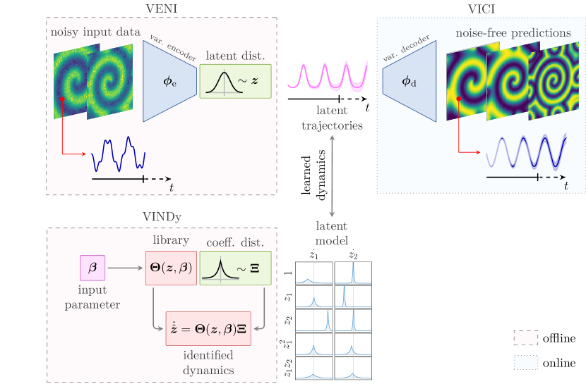
Figure 1: Overview of the VENI, VINDy, VICI procedure. High-dimensional, noisy data are mapped through a variational encoder to low-dimensional, latent random variables (VENI). Simultaneously, in a joint offline-training, the dynamics of the latent variables are learned by VINDy. Once this offline phase is concluded, noise-free, full-field solutions are computed through the online generative process together with the predictions uncertainty bounds (VICI).

The main contributions of the present work are:

1. We develop a novel data-driven system identification approach, referred to as VINDy, which is based on variational inference and incorporates uncertainty quantification.

2. We integrate dimensionality reduction (VENI), system identification (VINDy), and uncertainty quantification into a unified optimization framework that can be efficiently trained using a variational approach.

3. We demonstrate the potential of our approach through various examples, including a low-dimensional chaotic dynamical system and high-dimensional PDE benchmarks, highlighting the method’s ability to identify interpretable dynamics by retrieving the correct governing equations.

This paper is structured as follows. In Section 2 we detail the VENI, VINDy, VICI method in its components. We present how to perform the offline training and how to use the method to efficiently generate full-time solution. Then, we present the potential of the newly introduced VINDy method alone on the Rössler system, thus showcasing the methodology on a didactic, low-dimensional system with different noise intensities and sources (both model and measurement noise). Next we validate the performance of the complete framework through a series of high-dimensional PDE benchmarks, including a straight beam MEMS (Micro Electro-Mechanical System) resonator, which is excited at different forcing amplitudes and frequencies, and an unsteady PDE in fluid dynamics, consisting in a parametrised reaction-diffusion problem. Results for these numerical tests are showcased in Section 3, finally drawing some concluding remarks in Section 4. The source code of the proposed method is made available in the public repository https://github.com/jkneifl/VENI-VINDy-VICI.

2 Method

2.1 Problem setup

This work presents a method for data-driven system identification and for the efficient generation of solutions of nonlinear, parameterized, time-dependent partial differential equations (PDEs). In particular, we are interested in computing high-fidelity (spatial) approximations of the solutions over a set of $N$ spatial degrees of freedom, which usually come from suitable space discretizations techniques (such as, for instance, finite element, finite volume or isogeometric analysis methods) or represent measurement/sensor locations. The PDE system can then be expressed as a dynamical system of the form

$$\begin{cases}\dot{\bm{x}}(t;\bm{\beta})=\mathbf{F}(t,\bm{x}(t;\bm{\beta});\bm{\beta}),&t\in(0,T),\\ \bm{x}(0;\bm{\beta})=\bm{x}_{0},\end{cases}$$ (1)

where $\bm{x}\in\mathbb{R}^{N}$ is the state of the system, $\dot{\bm{x}}$ its derivative with respect to time $t$ and $\bm{\beta}=[\beta_{1},\ldots,\beta_{p}]^{\top}\in\mathbb{R}^{p}$ the vector collecting $p$ (possibly) time dependent parameters and/or forcing terms. The function $\mathbf{F}$ defines the dynamics of the physical system, evolving from the initial state $\bm{x}_{0}$. As the size $N$ is typically extremely large, system (1) is denoted as full order model (FOM).

Our goal is to compute uncertainty-aware predictions of the time evolution of solutions to (1), given a limited training set of noisy snapshots. We split the objective in two tasks: (i) construct a generative model that allows us to reproduce noise-free, full, spatial states of the system, and (ii) identify the system’s dynamics $\mathbf{F}$ in a probabilistic framework in order to predict the evolution of the states under uncertainty. However, solving these tasks in the high-dimensional space might be extremely complicated and computationally demanding. At the same time, the state dimension $N$ classically results from the numerical discretization scheme or represents measurement degrees of freedom, while often the solution manifold is of significant lower dimension. Consequently, we propose a reduced-order modeling technique that simultaneously reduces the problem’s dimensionality and provides a new set of coordinates better suited to represent the dynamics of the problem, also accounting for uncertainty quantification. More specifically, tasks (i)-(ii) are addressed respectively by the following steps:

1. VENI (Variational Encoding of Noisy Inputs). A generative model based on variational autoencoders (VAEs) is employed to encode the high-dimensional, noisy snapshots data into a more suitable, low-dimensional, latent representation.

2. VINDy (Variational Identification of Nonlinear Dynamics). A probabilistic dynamical model of the system is learned by a variational version of SINDy (Sparse Identification of Nonlinear Dynamics) [8] on the time series data expressed in the new set of latent coordinates.

Once these two operations are performed offline, we obtain a reduced-order model (ROM) within a probabilistic framework that integrates both the system dynamics and uncertainty quantification. The model can then be queried through an online procedure denoted as

1. VICI (Variational Inference with Certainty Intervals). Given new parameter/forcing values $\bm{\beta}$ and initial condition $\bm{x}_{0}$, the ROM enables the calculation of the temporal evolution of the system’s solution through variational inference on both the latent variable distribution and the dynamic model. This naturally provides an estimation of prediction reliability through certainty intervals.

The details about the VENI, VINDy, and VICI steps are explained in the following sections.

2.2 Variational Encoding of Noisy Inputs (VENI)

When relying on data to create models, one cannot assume perfect measurements, but must consider noise that reflects the complexity of the real world, the imperfection of measurements and the lack of knowledge. At the same time, including noise can lead to more robust models and equip them with the ability to cope with unexpected dynamic variations. Consequently, we consider a limited set of noisy snapshot data of a system $\mathbf{X}\coloneqq\{\bm{x}^{(i)}\}_{i=1}^{n_{s}}\in\mathbb{R}^{N}$, which correspond to $n_{s}$ observations distributed according to some unknown distribution $p_{\text{true}}(\bm{x})$ over $\mathbb{R}^{N}$ as starting point for our approach. The strategy of generative models is then to construct a probability distribution $p$, such that $p\approx p_{\text{true}}$. In order to achieve this goal, we make use of variational autoencoders (VAEs), introduced in [20] and comprehensively explained in [34]. VAEs allow variational inference for large datasets and can be used for uncertainty quantification, see [35, 36]. Moreover, they include terms in their objective function that encourage continuity and smoothness in the learned latent space. Accordingly, they allow us to control the way we can model our latent distributions through the choice of suitable priors [33, 26].

The use of autoencoders to create low-dimensional embeddings is justified by the basic assumption of reduced-order modeling: the solutions of PDEs usually lie on a low-dimensional manifold embedded in the high-dimensional, full order space. This allows us to introduce a set of low-dimensional, latent variables $\bm{z}=[z_{1},\ldots,z_{n}]^{\top}\in\mathbb{R}^{n}$, where typically $n\ll N$, from which it is possible to reconstruct the high-fidelity data $\bm{x}$. Specifically, we assume that each high-fidelity data $\bm{x}$ is generated from the latent variables $\bm{z}$ through a decoder mapping $\bm{\phi}_{\text{d}}(\cdot\,;\bm{W}_{\bm{\phi}_{\text{d}}})$, parametrised by a set of weights $\bm{W}_{\bm{\phi}_{\text{d}}}$. The decoder maps latent variables $\bm{z}$ into an output probability distribution over $\mathbb{R}^{N}$:

$$\bm{\phi}_{\text{d}}(\cdot\,;\bm{W}_{\bm{\phi}_{\text{d}}}):\mathbb{R}^{n}\rightarrow\mathcal{P},\text{ such that }\bm{z}\mapsto\bm{\phi}_{\text{d}}(\bm{z};\bm{W}_{\bm{\phi}_{\text{d}}})=~{}p(\bm{x}|\bm{z};\bm{W}_{\bm{\phi}_{\text{d}}}).$$ (2)

The output distribution is searched within a chosen family of distributions $\mathcal{P}$ on $\mathbb{R}^{N}$ and it is selected by optimizing $\bm{W}_{\bm{\phi}_{\text{d}}}$. The optimal parameters $\bm{W}_{\bm{\phi}_{\text{d}}}$ are obtained by maximizing the probability of each $\bm{x}$ in the training set $\mathbf{X}$ under the entire generative process

$$p(\bm{x})=\int_{\mathbb{R}^{n}}{p(\bm{x}|\bm{z}\,;\bm{W}_{\bm{\phi}_{\text{d}}})p(\bm{z})d\bm{z}},$$ (3)

where prior distributions on latent variables $p(\bm{z})$ are prescribed and can be chosen to be, for instance, Gaussian, Laplacian, etc. As the integral in (3) is not directly computable, variational methods rely on a sampling strategy which consists in first sampling a large number of $\bm{z}$ values $\{\bm{z}^{(1)},\ldots,\bm{z}^{(s)}\}$ from $p(\bm{z})$, and then approximating $p(\bm{x})\approx\frac{1}{s}\sum_{i=1}^{s}p(\bm{x}|\bm{z}^{(i)})$. However, as $\bm{x}$ is high-dimensional, this approach is computationally inefficient as it would require an extremely large number of samples $s$ before having an accurate estimate of $p(\bm{x})$.

VAEs aim to modify the sampling procedure by identifying, within a family of distributions $\mathcal{Q}$ on $\mathbb{R}^{n}$, a member $q$ which approximates the unknown posterior distribution $p(\bm{z}|\bm{x})$, such that $q$ can be sampled to generate values of $\bm{z}$ that are likely to have produced the snapshot $\bm{x}$. Therefore the idea is to learn an encoder $\bm{\phi}_{\text{e}}$, which maps snapshot data $\bm{x}$ into a probability distribution in $\mathcal{Q}$:

$$\bm{\phi}_{\text{e}}(\cdot\,;\bm{W}_{\bm{\phi}_{\text{e}}}):\mathbb{R}^{N}\rightarrow\mathcal{Q},\text{ such that }\bm{x}\mapsto\bm{\phi}_{\text{e}}(\bm{x};\bm{W}_{\bm{\phi}_{\text{e}}})=~{}q(\bm{z}|\bm{x};\bm{W}_{\bm{\phi}_{\text{e}}}).$$ (4)

The optimal parameters $\bm{W}_{\bm{\phi}_{\text{e}}}$ are obtained by minimizing the Kullback-Leibler (KL) divergence between the candidate distributions and target posterior distribution over $\mathcal{Q}$

$${\text{KL}\left(q(\bm{z}|\bm{x};\bm{W}_{\bm{\phi}_{\text{e}}})\parallel p(\bm{z}|\bm{x})\right)\coloneqq\mathbb{E}_{\bm{z}\sim q}\left[\log q(\bm{z}|\bm{x};\bm{W}_{\bm{\phi}_{\text{e}}})-\log p(\bm{z}|\bm{x})\right]},$$ (5)

which represents a measure of similarity between the two densities.

Applying Bayes’ theorem to $p(\bm{z}|\bm{x})$ in (5) we obtain

$$\text{KL}(q(\bm{z}|\bm{x})\parallel p(\bm{z}|\bm{x})) =\mathbb{E}_{\bm{z}\sim q}[\log q(\bm{z}|\bm{x})-\log p(\bm{z}|\bm{x})]=\mathbb{E}_{\bm{z}\sim q}[\log q(\bm{z}|\bm{x})-\log p(\bm{x}|\bm{z})-\log p(\bm{z})]+\log p(\bm{x})$$

$$=-\mathbb{E}_{\bm{z}\sim q}[\log p(\bm{x}|\bm{z})]+\text{KL}(q(\bm{z}|\bm{x})\parallel p(\bm{z}))+\log p(\bm{x}),$$

which can be rearranged and rewritten, using (2)-(4), as

$$\log p(\bm{x})-\text{KL}(q(\bm{z}|\bm{x})\parallel p(\bm{z}|\bm{x})) =\mathbb{E}_{\bm{z}\sim q}[\log p(\bm{x}|\bm{z})]-\text{KL}(q(\bm{z}|\bm{x})\parallel p(\bm{z}))$$ (6)

$$=\mathbb{E}_{\bm{z}\sim q}[\log\bm{\phi}_{\text{d}}(\bm{z})]-\text{KL}(\bm{\phi}_{\text{e}}(\bm{x})\parallel p(\bm{z})).$$ (7)

The left-hand side in (6) represents the quantities, introduced in (3)-(5), that we aim to optimize: the probability distribution at the observed training data $p(\bm{x})$ together with the error term between the approximated posterior distribution and the real one. This latter term makes the approximated posterior distribution $q(\bm{z}|\bm{x})$ able to produce $\bm{z}$ from which it is possible to reconstruct the given $\bm{x}$.

The equality (6) allows us to make this goal achievable in practice by providing a right-hand side that is computationally tractable. The term $\mathbb{E}_{\bm{z}\sim q}[\log p(\bm{x}|\bm{z})]$ in (6) ($\mathbb{E}_{\bm{z}\sim q}[\log\bm{\phi}_{\text{d}}(\bm{z})]$ in (7), respectively) expresses the reconstruction loss. It ensures that the log-probability of $\bm{x}$ given $\bm{z}$ drawn from the approximated posterior $q(\bm{z}|\bm{x})$ is maximized, ı.e., that the input is reconstructed well by the decoder $\bm{\phi}_{\text{d}}$ from a sample in the reduced space. The second term ensures that the approximated posterior $q(\bm{z}|\bm{x})$ is pushed closer to the prior, ı.e. that reduced coordinates identified by the encoder $\bm{\phi}_{\text{e}}$ respect the assumed prior over the latent variables $p(\bm{z})$. In the next section, we discuss how to properly select the class of encoder and decoder (in particular, the family of distributions $\mathcal{Q}$ and $\mathcal{P}$, respectively), such that their weights, $\bm{W}_{\bm{\phi}_{\text{e}}}$ and $\bm{W}_{\bm{\phi}_{\text{d}}}$, can be optimized using standard machine learning optimization techniques, such as stochastic gradient ascent.

2.2.1 Choice of encoder and decoder

In this work, the choice of family of output distribution $\mathcal{P}$ for decoder is Gaussian, ı.e., given $\bm{z}$, we have

$$\bm{\phi}_{\text{d}}(\bm{z};\bm{W}_{\bm{\phi}_{\text{d}}})=p(\bm{x}|\bm{z};\bm{W}_{\bm{\phi}_{\text{d}}})=\mathcal{N}\left(\bm{\mu}_{\bm{\phi}_{\text{d}}}(\bm{z};\bm{W}_{\bm{\phi}_{\text{d}}}),\sigma^{2}\bm{I}_{N}\right),$$ (8)

where the mean $\bm{\mu}_{\bm{\phi}_{\text{d}}}\in\mathbb{R}^{N}$ is implemented by multi-layer, feed-forward, neural network, while the covariance is an isotropic matrix with variance $\sigma^{2}$ (scalar hyperparameter). Even though any probability distribution continuous in $\bm{W}_{\bm{\phi}_{\text{d}}}$ can be employed, the advantage of using an isotropic Gaussian distribution is that, the term $\mathbb{E}_{\bm{z}\sim q}[\log\bm{\phi}_{\text{d}}(\bm{z})]$ in (7) is proportional to the squared distance between the neural network reconstruction $\hat{\bm{x}}\coloneqq\bm{\mu}_{\bm{\phi}_{\text{d}}}(\bm{z};\bm{W}_{\bm{\phi}_{\text{d}}})$ and the original data $\bm{x}$ [34]. In this way, the decoder can be trained on the classical reconstruction loss of standard autoencoders: $\norm{\bm{x}-\hat{\bm{x}}}_{2}^{2}$.

On the other hand, for the output candidate posterior distributions $\mathcal{Q}$ of the encoder $\bm{\phi}_{\text{e}}$, we consider the same family as the prior assumed on the latent variables, but where the parameters of the distribution are again determined by a neural network. For instance, if we assume as prior that the latent variables are independent, standard gaussians, ı.e. $p(\bm{z})=\mathcal{N}(\bm{0},\bm{I}_{n})$, the encoder network returns the mean values $\bm{\mu}_{\bm{\phi}_{\text{e}}}~{}\in~{}\mathbb{R}^{n}$ and variances $\bm{\delta}_{\bm{\phi}_{\text{e}}}\in\mathbb{R}^{n}_{+}$ describing the posterior

$$\bm{\phi}_{\text{e}}(\bm{x};\bm{W}_{\bm{\phi}_{\text{e}}})=q(\bm{z}|\bm{x}\mathcal{;}\bm{W}_{\bm{\phi}_{\text{e}}})=\mathcal{N}\left(\bm{\mu}_{\bm{\phi}_{\text{e}}}(\bm{x};\bm{W}_{\bm{\phi}_{\text{e}}}),\text{diag}(\bm{\delta}_{\bm{\phi}_{\text{e}}}(\bm{x};\bm{W}_{\bm{\phi}_{\text{e}}}))\right),$$ (9)

where $\text{diag}(\bm{\delta}_{\bm{\phi}_{\text{e}}})\in\mathbb{R}^{n\times n}$ indicates the diagonal matrix having $\bm{\delta}_{\bm{\phi}_{\text{e}}}$ on the main diagonal. This choice is advantageous, as the term $\text{KL}(\bm{\phi}_{\text{e}}(\bm{x})|p(\bm{z}))$ in (7) can be then written in closed-form for distributions such as Gaussian and Laplacian (see A.2).

2.3 Variational Identification of Nonlinear Dynamics (VINDy)

Despite the VAEs’ capabilities in identifying low-dimensional variables from which the high-dimensional distribution can be generated, they do not account for time or dynamics. Consequently, introducing a VAE in a reduced-order modeling setting is just the first step in the task of approximating (1). The second step must involve a strategy to describe the latent dynamics and evolve them in time. Hence, we aim to identify a dynamic system of the form

$$\begin{cases}\dot{\bm{z}}(t;\bm{\beta})={\mathbf{f}}(t,\bm{z}(t;\bm{\beta});\bm{\beta}),&t\in(0,T),\\ \bm{z}(0;\bm{\beta})=\bm{z}_{0},\end{cases}$$ (10)

in the new set of latent coordinates $\bm{z}\in\mathbb{R}^{n}$, where $\bm{z}_{0}\sim\bm{\phi}_{\text{e}}(\bm{x}_{0})$ and $\dot{\bm{z}}$ represent the latent states’ time derivatives. In particular, we are interested in identifying the unknown function $\mathbf{f}$ that encodes the dynamics of the low-dimensional system. A popular as well as powerful method to do so is Sparse Identification of Nonlinear Dynamics (SINDy) [8], which assumes that $\mathbf{f}$ can be expressed as a sparse combination of a predefined set of candidate functions.

SINDy

SINDy aims to approximate the latent dynamics $\mathbf{f}$ in (10) as the product of a library of $r$ candidate functions $\bm{\Theta}(\bm{z},\bm{\beta})\in\mathbb{R}^{r}$ and corresponding coefficients $\bm{\Xi}\in\mathbb{R}^{r\times n}$ resulting in

$$\dot{\bm{z}}=\mathbf{f}(\bm{z},\bm{\beta})\approx\bm{\Theta}(\bm{z},\bm{\beta})\bm{\Xi}.$$ (11)

To construct a suitable right-hand side, $r$ potentially useful basis functions, such as polynomial or trigonometric functions are considered. For instance, $\bm{\Theta}(\bm{z},\bm{\beta})=[1,z_{1},z_{1}^{2},z_{2}\beta_{1}\dots,\sin(z_{1}),\beta_{1}\cos(z_{2}),\dots]$. The choice of the candidate functions is typically guided by a possible prior knowledge of the physical system and of the parameter/forcing dependency. The unknown coefficients which determines the active terms from $\bm{\Theta}$ in $\mathbf{f}$ are collected in the matrix $\bm{\Xi}$ and estimated by sparse regression.

VINDy

We transfer this idea into a probabilistic setting so that uncertainty quantification of the coefficients $\bm{\Xi}$ is directly possible. In detail, we introduce a method that we refer to as Variational Identification of Nonlinear Dynamics (VINDy) that adapts the ideas behind VAEs to system identification. We assume that $\dot{\bm{z}}$ depend on some random process that is defined by unknown probability distributions of the coefficients $\bm{\Xi}$, with a given prior $p(\bm{\Xi})$ over $\mathbb{R}^{r\times n}$. The entries $\Xi_{ij}$, are independent scalar variables determining the contribution of the $i$-th function candidate to the $j-$th equation of system (11), defining the dynamics of $z_{j}$. While the goal in VAEs is to maximize the log-probability of $p(\bm{x})$, in VINDy we aim to maximize the probability of the latent time derivatives $p(\dot{\bm{z}})$. Moreover, similar to VAE, where we assumed that the high-dimensional states $\bm{x}$ are generated from the latent variables $\bm{z}$, here, our target quantity $\dot{\bm{z}}$ can be interpreted as being generated from $\bm{\Xi}$ and $\bm{z}$ following (11). In particular, we assume

$$\dot{\bm{z}}|\bm{\Xi},\bm{z}\sim\mathcal{N}\left(\bm{\Theta}(\bm{z},\bm{\beta})\bm{\Xi},\tilde{\sigma}^{2}\bm{I}\right),$$ (12)

where $\tilde{\sigma}^{2}$ is a scalar hyperparameter, and we approximate the unknown posterior distribution $p(\bm{\Xi}|\dot{\bm{z}})$ with $q(\bm{\Xi}|\dot{\bm{z}})$, searched within a suitable family $\tilde{\mathcal{Q}}$. In particular, we use distribution families $\tilde{\mathcal{Q}}$ that are parameterizable with a set of trainable weight matrices of dimension $r\times n$, that is $\bm{W}_{\bm{\Xi}}=\{{\bm{W}}_{\bm{\Xi}_{\bm{\mu}}},{\bm{W}}_{\bm{\Xi}_{\bm{\delta}}}\}$. The entries ${W}_{\bm{\Xi}_{\bm{\mu}}}^{ij},{W}_{\bm{\Xi}_{\bm{\delta}}}^{ij}$ directly define the distribution parameters of $\Xi_{ij}$. For example, they can represent the mean and variance for a Gaussian distribution $\Xi_{ij}\sim\mathcal{N}({W}_{\bm{\Xi}_{\bm{\mu}}}^{ij},{W}_{\bm{\Xi}_{\bm{\delta}}}^{ij})$ or the localization parameter and scale factor in case of a Laplace distribution $\Xi_{ij}\sim\mathcal{L}({W}_{\bm{\Xi}_{\bm{\mu}}}^{ij},{W}_{\bm{\Xi}_{\bm{\delta}}}^{ij})$. In contrast to Gaussian priors, Laplacian priors can act as sparsity-promoting regularization terms within a regression task [26]. Consequently, they are more prone to provide a parsimonious dynamical model. More detailed information on the choice of distribution families can be found in A.2.
Note that the distribution parameters of the approximated posterior for $\bm{\Xi}$ do not feature an explicit dependency on the conditioning variable $\dot{\bm{z}}$. This differs from the posteriors approximated by the encoder and decoder distributions for which their conditioning variables ($\bm{x}$ and $\bm{z}$, respectively) are explicit inputs of the neural network defining their statistical moments (see (8)-(9)). To highlight this difference, in the following, we indicate the posterior $q(\bm{\Xi}|\dot{z};\bm{W}_{\bm{\Xi}})$ simply as $q(\bm{\Xi})$. In the same way as $q(\bm{\Xi})$, we may approximate the posterior on the latent variables $q(\bm{z})$ with a distribution parameterized by trainable weights.

Analogously to the objective (6) derived for the VAE, in order to find the coefficient distributions explaining the observed dynamics, we maximize the log-probability of the latent derivatives $\dot{\bm{z}}$, while reducing the error of approximating the posteriors for $\bm{\Xi}$ and $\bm{z}$, that is

$$\begin{split}\log p(\dot{\bm{z}})&-\text{KL}(q(\bm{\Xi})\parallel p(\bm{\Xi}|\dot{\bm{z}}))-\text{KL}(q(\bm{z})\parallel p(\bm{z}|\dot{\bm{z}}))=\\ &=\mathbb{E}_{\bm{\Xi}\sim q(\bm{\Xi})}\left[\log(p(\dot{\bm{z}}\mid\bm{\Xi},\bm{z}))\right]-\text{KL}(q(\bm{\Xi})\parallel p(\bm{\Xi}))-\text{KL}(q(\bm{z})\parallel p(\bm{z})).\end{split}$$ (13)

This theoretical objective is translated into practically computable quantities (right-hand side of (13)) as explained in A.1. In the next session we explain how VENI and VINDy steps can be performed together in an unified training.

2.4 Offline Training

As discussed above, our proposed strategy features the generation of a set of reduced variables and the identification of the dynamics in this latent description, by employing VENI and VINDy respectively. So far these tasks are addressed individually by optimizing the objective functions (7) and (13). However, the possibility of identifying parsimonious, accurate dynamical models strongly depends on the choice of reduced coordinates [17, 16], and the ones provided by VENI are not necessarily optimal, as VAEs do not take dynamics into account. Moreover, objectives of VENI and VINDy partially overlap as both aim to approximate a suitable distribution $q$ for the latent variables. This motivates us to solve VENI and VINDy simultaneously in an unified offline training, which consists in solving

$$\underset{\bm{W}_{\bm{\phi}_{\text{e}}},\bm{W}_{\bm{\phi}_{\text{d}}},\bm{W}_{\bm{\Xi}}}{\max}\mathbb{E}_{\bm{x}\sim\mathbf{X}}\left[\underbrace{\mathbb{E}_{\bm{z}\sim q(\bm{z}|\bm{x})}[\log\bm{\phi}_{\text{d}}(\bm{z})]}_{\text{\small Reconstruction}}-\underbrace{2\text{KL}(\bm{\phi}_{\text{e}}(\bm{x})\parallel p(\bm{z}))}_{\text{\small Posterior for $\bm{z}$}}+\underbrace{\mathbb{E}_{\bm{\Xi}\sim q(\bm{\Xi})}\left[\log(p(\dot{\bm{z}}\mid\bm{\Xi},\bm{z}))\right]}_{\text{\small Latent dynamics}}+\underbrace{\text{KL}(q(\bm{\Xi})\parallel p(\bm{\Xi}))}_{\text{\small Posterior for $\bm{\Xi}$}}\right].$$ (14)

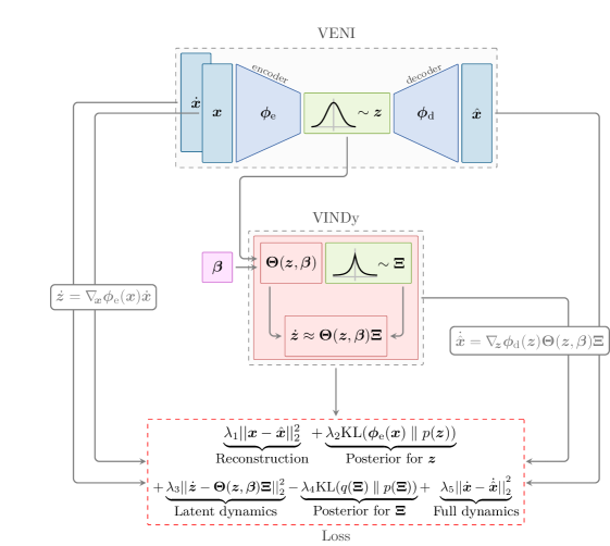
Figure 2: Schematic representation of the offline training consisting in the VENI and VINDy steps. The encoder maps the snapshot data $\bm{x}$ into the corresponding posterior distributions $\bm{\phi}_{\text{e}}(\bm{x})$, from which we sample the latent states $\bm{z}$. Latent states are passed to both the decoder and VINDy setup. The decoder outputs the distribution of the reconstruction of the full order state given $\bm{z}$.While in VINDy we first sample the coefficients $\bm{\Xi}$ of the dynamical model from the posterior $q(\bm{\Xi})$ and then, together with the sample $\bm{z}$ and parameters $\bm{\beta}$, they form the posterior distribution of the latent derivatives.

The optimization function above represents the mean value of all terms appearing in (7) and (13) over the training dataset $\mathbf{X}$, where the VINDy latent posterior $q(\bm{z})$ has been replaced by the VAE latent posterior $\bm{\phi}_{\text{e}}(\bm{x})$, since we require to approximate a single posterior from which to sample.
The offline training procedure is detailed and illustrated in Fig. 2. Following this strategy, we simultaneously learn the distribution of the dynamic coefficients $\bm{\Xi}$, together with the encoder $\bm{\phi}_{\text{e}}$ and decoder $\bm{\phi}_{\text{d}}$ distributions. Since both encoder and decoder are defined by neural networks with coefficients $\bm{W}_{\bm{\phi}_{\text{e}}}$ and $\bm{W}_{\bm{\phi}_{\text{d}}}$, and the distribution of $\bm{\Xi}$ is parametrised by trainable weights $\bm{W}_{\bm{\Xi}}$, it is the straightforward to learn all the unknown coefficients $\bm{W}_{\bm{\phi}_{\text{e}}},\bm{W}_{\bm{\phi}_{\text{d}}},\bm{W}_{\bm{\Xi}}$ via backpropagation, using standard gradient-based methods as, e.g., ADAM [37]. The only arrangement we have to take is the standard reparameterization trick in VAEs [20, 38] to allow backpropagation of (14) through the networks. Indeed, sampling $\bm{z}$ directly from the distribution defined by the encoder is not a differentiable operation, thus has no gradient. In the case the family of distributions $\mathcal{Q}$ for the encoder is chosen as Gaussian, a noise term $\bm{\zeta}\sim\mathcal{N}(\bm{0},\bm{I})$ acting as additional input, which is not parameterized by the network, is introduced whereby a sample can be drawn following

$$\bm{z}=\bm{\mu}_{\bm{\phi}_{\text{e}}}(\bm{x})+\bm{\zeta}*\bm{\delta}_{\bm{\phi}_{\text{e}}}(\bm{x}),$$ (15)

where $*$ indicates the element-wise product. This trick holds for any family of distributions closed under linear transformations, e.g., Laplace, by changing the distribution of $\bm{\zeta}$ accordingly. From (15), it follows that a sample for the latent state derivatives can be obtained by applying chain rule to the full-state derivatives

$$\dot{\bm{z}}=\nabla_{\bm{x}}\bm{\mu}_{\bm{\phi}_{\text{e}}}(\bm{x})\dot{\bm{x}}+\bm{\zeta}*\nabla_{\bm{x}}\bm{\delta}_{\bm{\phi}_{\text{e}}}(\bm{x})\dot{\bm{x}}.$$ (16)

We conclude the section by presenting how to computationally solve the optimization problem (14). Thanks to the assumptions and choices on the family of distributions, the general, probabilistic objective (14) can be translated into the following practical, data-driven optimization problem

$$\underset{\bm{W}_{\bm{\phi}_{\text{e}}},\bm{W}_{\bm{\phi}_{\text{d}}},\bm{W}_{\bm{\Xi}}}{\max}\frac{1}{n_{s}}\sum_{i=1}^{n_{s}}\underbrace{\lambda_{1}||{\bm{x}^{(i)}-\hat{\bm{x}}^{(i)}}||_{2}^{2}}_{\text{\small Reconstruction}}+\underbrace{\lambda_{2}\text{KL}(\bm{\phi}_{\text{e}}(\bm{x}^{(i)})\parallel p(\bm{z}))}_{\text{\small Posterior for $\bm{z}$}}+\underbrace{\lambda_{3}{\norm{\dot{\bm{z}}^{(i)}-\bm{\Theta}(\bm{z}^{(i)},\bm{\beta})\bm{\Xi}^{(i)}}}_{2}^{2}}_{\text{\small Latent dynamics}}-\underbrace{\lambda_{4}\text{KL}(q(\bm{\Xi})\parallel p(\bm{\Xi}))}_{\text{\small Posterior for $\bm{\Xi}$}}+\underbrace{\lambda_{5}||{\dot{\bm{x}}^{(i)}-\dot{\hat{\bm{x}}}^{(i)}||}_{2}^{2}}_{\text{\small Full dynamics}}$$ (17)

where the expectation is approximated by the sample mean over the training set. We recall that $\bm{x}^{(i)}$ and $\dot{\bm{x}}^{(i)}$ indicate the full state and time derivatives of the $i-$th training snapshot; $\bm{z}^{(i)},\dot{\bm{z}}^{(i)}$ are the latent counterparts, sampled via (15) and (16), respectively; while $\bm{\Xi}^{(i)}$ is a sample drawn from the approximated posterior $q(\bm{\Xi})$. As anticipated in section 2.2.1, the reconstruction loss in (14) is proportional to the squared euclidean distance between the data $\bm{x}^{(i)}$ and the decoder mean $\hat{\bm{x}}^{(i)}=\bm{\mu}_{\bm{\phi}_{\text{d}}}(\bm{z}^{(i)};\bm{W}_{\bm{\phi}_{\text{d}}})$, since we assumed isotropic gaussian distribution for the decoder (see (8)) [34]. For the exact same reason, as the posterior distribution of $\dot{\bm{z}}$ has the same characteristics (see (12)), the latent dynamics loss can be rewritten here as proportional to ${\norm{\dot{\bm{z}}^{(i)}-\bm{\Theta}(\bm{z}^{(i)},\bm{\beta})\bm{\Xi}^{(i)}}}_{2}^{2}$. Moreover, as suggested in [17], an additional full-dynamics term is included as regularization to account for consistency between the real time derivatives of the data, $\dot{\bm{x}}^{(i)}$, and the mean value of their reconstruction from the approximated latent derivatives, that is $\dot{\hat{\bm{x}}}^{(i)}\coloneqq\nabla_{\bm{z}}\bm{\mu}_{\bm{\phi}_{\text{d}}}(\bm{z}^{(i)})\bm{\Theta}(\bm{z}^{(i)},\bm{\beta})\bm{\Xi}^{(i)}$. Finally, given the assumption that the families of distributions for the posteriors $q(\bm{\Xi}|\dot{\bm{z}}^{(i)})$ and $q(\bm{z}|\bm{x}^{(i)})$ (that is $\bm{\phi}_{\text{e}}(\bm{x}^{(i)})$) are the same of those of the priors (in the cases of Gaussian and Laplacian distributions), the KL divergences in (17) can be expressed in closed-form and computed directly from the statistical moments of the posteriors (see A.2). By minimizing the divergences, the posteriors are pushed closer to the selected priors which helps minimizing the optimization goal formulated in (7) and (13).
The weighting coefficients $\{\lambda_{i}\}_{i=1}^{5}\in\mathbb{R}^{+}$ are hyperparameters, which account for the proportionality constants and determine the contribution of each term. As a general guideline for selecting these hyperparameters, the dominant terms are those related to the reconstruction and identification of the latent dynamics, ı.e., $\lambda_{1}$ and $\lambda_{3}$. Thus, they should be kept orders of magnitude larger than $\lambda_{2}$, $\lambda_{4}$, and $\lambda_{5}$, which weight the remaining regularization terms. In cases where the method converges to latent variables of very small magnitudes, the latent dynamics loss might appear low due to the small magnitudes rather than correct identification of the dynamics. To address this, $\lambda_{5}$ can be increased so that the full dynamics term ensures the identified dynamics are respected on the original variables, thus mitigating this scaling issue. Regarding the KL-losses, a prioritized weighting of these terms might be used, as done for $\beta-$VAEs [39], to encourage more efficient latent encoding and disentanglement of the latent coordinates. In general, the precise hyperparameter values need to be adjusted to the specific dataset at hand, as the choice of hyperparameters is problem-dependent and their regulation could improve the training convergence. In addition, it would also be possible to use constrained learning [40] so that, for example, dynamics are only learned in an area where satisfactory reconstruction is achieved.

2.5 Variational Inference with Certainty Intervals (VICI)

Thanks to the probabilistic framework, the proposed method seamlessly incorporates uncertainty quantification (UQ), following directly from the model’s approximated posterior distributions. First of all, the approximated distribution over the dynamic coefficients $q(\bm{\Xi})$ provides insights on which terms are active in the library, what is their contributions to the dynamics, and the variability and reliance on the estimates. This enables the incorporation of model uncertainty in the data generative process. On the other hand, the method effectively addresses and quantifies measurement noise, as noisy training data $\bm{x}$ are processed by encoder networks and mapped into probability distributions $q(\bm{z}|\bm{x})=\bm{\phi}_{\text{e}}(\bm{x})$.

Once the offline phase is complete, the fitted model can be used queried online to generate solutions for unseen initial conditions $\bm{x}_{0}$ and input parameters $\bm{\beta}$. The probabilistic setup, in addition to allow for offline quantification of model and measurement noise, can be exploited to perform UQ on the predicted solutions. In particular, we employ a sampling-based approach to construct uncertainty intervals for the time evolution of the estimated solution.

For a given initial condition $\bm{x}_{0}$ in the full space, we sample, from the approximated posteriors, $m$ latent initial conditions, ı.e. $\{\bm{z}_{0}^{(i)}\}_{i=1}^{m}\stackrel{{\scriptstyle\text{iid}}}{{\sim}}\bm{\phi}_{\text{e}}(\bm{x}_{0})$ and coefficients $\{\bm{\Xi}^{(i)}\}_{i=1}^{m}\stackrel{{\scriptstyle\text{iid}}}{{\sim}}q(\bm{\Xi})$. Then, for each pair $(\bm{z}_{0}^{(i)},\bm{\Xi}^{(i)})$, we use standard time stepping schemes, such as Runge-Kutta methods, to evolve the system of ordinary differential equations (ODEs) $\dot{\bm{z}}=\bm{\Theta}(\bm{z},\bm{\beta})\bm{\Xi}^{(i)}$ from the initial condition $\bm{z}_{0}^{(i)}$ over a set of discrete time-steps $\mathcal{T}=\{0,t_{1},\ldots,T\}$. Finally the so-computed latent trajectories $\{\bm{z}^{(i)}(t):t\in\mathcal{T}\}_{i=1}^{m}$ are passed to the decoder mean which outputs the full state solution trajectories $\{\hat{\bm{x}}^{(i)}(t)=\bm{\mu}_{\bm{\phi}_{\text{d}}}(\bm{z}^{(i)}(t)):t\in\mathcal{T}\}_{i=1}^{m}$. Note that we avoid sampling at each time step $t$ from the corresponding posterior $\bm{x}^{(i)}(t)\sim\bm{\phi}_{\text{d}}(\bm{z}^{(i)}(t))$, in order to preserve in the full space (possible) regularity properties in time of the latent trajectories. Uncertainty bounds for the approximated solution are then computed from the statistical moments of the set of $m$ trajectories.

The VICI procedure is illustrated in Fig. 3. This testing approach differs from standard generative procedures of VAE, where usually the encoder is ignored at testing and new solutions are generated directly from the latent variables sampled from the prior. In our framework we are taking into account time and dynamics, thus the encoder is fundamental to accurately approximate the latent distribution of the initial condition.

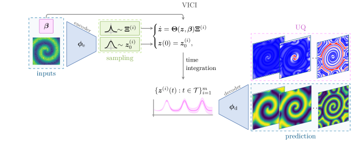
Figure 3: Schematic representation of the online VICI procedure to generate new solutions for a given initial condition $\bm{x}_{0}$ and set of parameters $\bm{\beta}$. We first sample multiple instances of the corresponding latent initial conditions and coefficients of the dynamical model, each defining an ODE system. Then each dynamical system is integrated in time through standard time-stepping schemes, resulting in multiple latent trajectories. These latent trajectories are finally processed by the decoder mean to obtain full state trajectories. Predictions and the corresponding UQ are computed directly from the statistical properties of the approximated solution trajectories.

2.5.1 Sparsity promotion by zero-pdf thresholding

A further advantage of modeling the coefficients of the reduced dynamics as random variables is that one can select the relevant coefficients and discard the remainings according to their identified probability density function (pdf). The idea is to only keep those terms whose pdf is below a given threshold, ı.e.  $\text{pdf}_{\mathcal{L}}(0)<\tau$. In contrast to sequential thresholding [8], this does not necessarily penalise coefficients which are small in magnitude, as they can have small pdf values at zero, as long as their identified variance is low. Instead coefficients whose distributions are centered around zero with larger variances, that consequently do not have a clear and consistent contribution to the dynamics, are canceled. The threshold value $\tau$ is a hyperparameter that can be tuned to adjust the sparsity of the identified system.

3 Numerical examples

3.1 Numerical example I: Rössler System

In order to assess the potential of our novel VINDy approach alone, we first test the methodology on a low-dimensional system. Consequently, no autoencoder is present and the VINDy method directly operates on the original system description. We consider the Rössler system for this validation. It is a set of ordinary differential equations defined as

$$\begin{split}\dot{z_{1}}&=-z_{2}-z_{3},\\ \dot{z_{2}}&=z_{1}+\alpha_{1}z_{2},\\ \dot{z_{3}}&=\alpha_{2}+z_{3}(z_{1}-\alpha_{3}),\end{split}$$ (18)

where $\bm{z}=[z_{1},z_{2},z_{3}]^{\intercal}$ is the vector of the system states and $\bm{\alpha}=[\alpha_{1},\alpha_{2},\alpha_{3}]^{\intercal}$ contains the system parameters.

Dataset

The data used to train our model consists of multiple simulations with parameters $\alpha_{1}=0.2,$ $\alpha_{2}=0.2,$ and $\alpha_{3}=5.7$ as well as normal randomly distributed initial conditions $\bm{z}(t_{0})\sim\mathcal{N}([-5,-5,0]^{\intercal},\sigma^{2}\bm{I})$ with a standard deviation of $\sigma=2.25$. We consider two sources of uncertainty: measurement noise and model noise. For the former we apply multiplicative noise to the state measurements, ı.e. $\bm{z}_{\text{noise}}(t)=\varepsilon\bm{z}(t)$ with $\varepsilon\sim\mathcal{L}\mathcal{N}(\bm{0},\lambda_{\varepsilon}*\bm{I})$ drawn from a log-normal distribution individually for every sample. The time derivatives are numerically computed from those noisy samples. The model uncertainty is realized as noise in the model parameters which are drawn from a normal distribution $\bm{\alpha}\sim\mathcal{N}([\alpha_{1},\alpha_{2},\alpha_{3}]^{\intercal},[\sigma_{\alpha_{1}}^{2},\sigma_{\alpha_{2}}^{2},\sigma_{\alpha_{3}}^{2}]^{\intercal})$ centered around the correct values with standard deviations $\sigma_{\alpha_{1}}=\lambda_{\alpha}{\alpha_{1}}$, $\sigma_{\alpha_{2}}=\lambda_{\alpha}{\alpha_{2}}$, and $\lambda_{\alpha}\sigma_{\alpha_{3}}={\alpha_{3}}$. The test data consists of a set of simulation that differs in its initial conditions from the training data and uses the correct parameter values.

Model

For the VINDy layer, we use a polynomial library $\bm{\Theta}(\bm{z})\in\mathbb{R}^{10}$ of order 2 including bias and interactions with Laplacian priors $\bm{\Xi}_{ij}\sim\mathcal{L}(0,1)$ for the corresponding coefficients. We train the model over 2000 epochs using early stopping. At the end of the training all coefficients $\bm{\Xi}_{ij}$ with a probability density function above a threshold of $pdf_{\bm{\Xi}_{ij}}(0)>5$ are set to zero.

Experiments and Results

We perform six experiments to measure the performance of VINDy: (a) One on noise-free data, two with model noise ((b) moderate $\lambda_{\alpha}=0.1$, (c) high $\lambda_{\alpha}=0.2$), two with measurement noise ((d) moderate $\lambda_{\varepsilon}=0.05$, (e) high $\lambda_{\varepsilon}=0.1$), and (f) one where both sources of uncertainty are taken into account. The impact of the respective noise on the training data can be seen in Fig. 4. For each training data set, we apply VINDy and sample from the resulting coefficient distributions to perform a sample-based UQ on the time evolution of the system states. As shown in Fig. 4, the resulting trajectories for no noise (a) and moderate model noise (b) follow the ground-truth quite well and capture the system dynamics. As expected, higher model noise leads to broader uncertainty bounds around the predicted mean trajectories. Nevertheless, even for high model noise (c) the identified system is able to follow the reference. This also holds true for moderate measurement noise (d) and the approach is only pushed to its limits for high measurement noise (e) and the combination of both noises (f). In those cases the state trajectories differ from the ground truth. However, even in these cases, the method extracts essential knowledge from the data, which becomes apparent upon looking at the identified coefficient distributions.

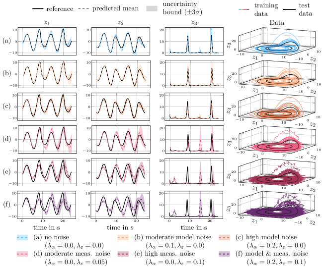
Figure 4: Temporal evolution of the Rössler system states including UQ for a test scenario on various noise scenarios. The corresponding training data for each scenario is shown at the right of the state trajectories.

As shown in Fig. 5, our method keeps all the important terms that originally appear in the underlying equation without relevance what kind of uncertainty is present in the data, i.e. for all noise levels. At the same time, most of the other irrelevant coefficients are centered around zero. For moderate noise level, the resulting coefficient distributions center around the reference value with high confidence, whereas higher noise levels lead to more conservative estimates and wider distributions.

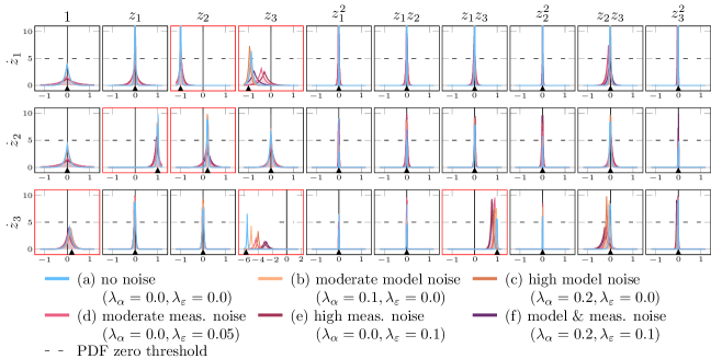
Figure 5: Distributions of coefficients identified for the Rössler system based on noise-free and noisy training data. The correct values are marked with a triangle at the bottom of each axis. All values that occur in the original equations are highlighted with red axes.

3.2 Numerical example II: Reaction-diffusion problem

We consider a reaction-diffusion system governed by equations

$$\dot{u}=\left(1-\left(u^{2}+v^{2}\right)\right)u+\mu\left(u^{2}+v^{2}\right)v+d_{1}\left(u_{xx}+u_{yy}\right),$$ (19)

$$\dot{v}=-\mu\left(u^{2}+v^{2}\right)u+\left(1-\left(u^{2}+v^{2}\right)\right)v+d_{2}\left(v_{xx}+v_{yy}\right),$$

where $\mu=1.0$ and $d_{1}=d_{2}=0.01$ are coefficients that respectively regulate the reaction and diffusion behaviors of the system. The problem is defined over a spatial domain $[-L,L]^{2}$ for $L=10$ and a time span $t\in[0,T]$ for $T=40$, periodic boundary conditions are prescribed, and the initial condition is defined as

$$u(x,y,0;\beta)=v(x,y,0;\beta)=\tanh{\left(\beta\sqrt{x^{2}+y^{2}}\cos{\left((x+iy)-\beta\sqrt{x^{2}+y^{2}}\right)}\right)}\,,$$ (20)

depending on the parameter $\beta\in\mathcal{P}=[0.7,1.1]$. System (19) generates spiral waves, which represent an attracting limit cycle in the state space [41] and whose radius is modulated by the parameter $\beta$.

Our goal is to create a generative model to compute the entire space–time solution for a new instance of parameter $\beta$.

Dataset

A grid of $N_{\beta}=20$ values for the parameter $\beta$ equispaced over $\mathcal{P}$ is considered. The parameter values are randomly partitioned in training and testing subsets, $\mathcal{P}_{\text{train}}$ and $\mathcal{P}_{\text{test}}$, such that $N_{\beta}^{\text{train}}=|\mathcal{P}_{\text{train}}|=16$ and $N_{\beta}^{\text{test}}=|\mathcal{P}_{\text{test}}|=4$. For each choice of $\beta$, numerical solutions for $u$ and $v$ are computed by solving the PDEs (19) with initial condition (20) by using the Fourier spectral method [42] with time step $\Delta t=0.05$ on an equispaced spatial grid with spatial step $\Delta h=0.4$. For the training set, solutions are computed over a limited time window $T_{\text{train}}=20$, while testing data reach final time $T=40$. Moreover, training data are corrupted by $20\%$ log-normal multiplicative noise to simulate measurement noise. Training and testing snapshots are stacked respectively in matrices $\mathbf{X}_{\text{train}}\in\mathbb{R}^{N_{t}^{\text{train}}N_{\beta}^{\text{train}}\times N}$ and $\mathbf{X}_{\text{test}}\in\mathbb{R}^{N_{t}^{\text{test}}N_{\beta}^{\text{test}}\times N}$, where $N_{t}^{\text{train}}=400$ and $N_{t}^{\text{test}}=800$ are the number of samples for training and testing sets respectively, and $N=2500$ is the number of spatial degrees of freedom. We preliminary reduce system dimension to $N_{\text{POD}}=32$ by projecting both training and testing data onto the reduced basis obtained using POD on $\mathbf{X}_{\text{train}}$. Projected data are denoted as $\tilde{\mathbf{X}}_{\text{train}}\in\mathbb{R}^{N_{t}^{\text{train}}N_{\beta}^{\text{train}}\times N_{\text{POD}}}$ and $\tilde{\mathbf{X}}_{\text{test}}\in\mathbb{R}^{N_{t}^{\text{test}}N_{\beta}^{\text{test}}\times N_{\text{POD}}}$.

Model

Regarding the VENI structure, the encoder consists out of a feed-forward neural network with 3 hidden dense layer of 32, 16 and 8 units, while the decoder network has a symmetrical structure. Spiral waves generated by the system (19) can be approximately captured by two oscillating spatial modes [17], thus we set the number of latent variables $n=2$. For VINDy, we employ a set of polynomial functions of the latent variables $\mathbf{z}=\left[z_{1},z_{2}\right]^{\top}$ up to the third degree with interaction and bias. No parametric dependency is included in the library, as parameter $\beta$ affects solely the initial conditions. Regarding the choice of prior distributions on the latent variables and on the VINDy coefficients, we consider gaussian and laplacian distributions, respectively, namely $\mathbf{z}\sim\mathcal{N}(\mathbf{0},\bm{I})$ and $\bm{\Xi}_{ij}\sim\mathcal{L}(0,1)$ for each entry.

Experiments and Results

The offline training is performed on the dataset $\{\tilde{\mathbf{X}}_{\text{train}},\dot{\tilde{\mathbf{X}}}_{\text{train}}\}$. The resulting posterior distributions for the model coefficients are depicted in Fig. 6. The primary dynamics of this phenomenon exhibit the characteristics of a linear oscillator, which our method successfully captures by identifying the linear coefficients as significant terms with high confidence. These coefficients are distinguished by a posterior mean significantly deviating from zero and a notably narrow variability, confirming their critical role in the observed dynamics. Moreover, our approach encourages parsimony in the dynamics by effectively setting to zero mean most nonlinear terms. Fig. 6 also presents the phase space representation in the identified latent coordinates, showcasing the oscillatory pattern and the attracting limit cycle. This demonstrates not only the effectiveness of our method but also its ability to preserve interpretable insights into the latent space.

To assess the accuracy and reliability of our method in making predictions, we evaluate its performance on the test set using the VICI approach. For initial conditions not seen during training and corresponding to test parameter instances, we predict the approximate solutions up to a final time of $T=40$. These predictions are compared with the noise-free, numerical values ${\mathbf{X_{\text{test}}}}$. Fig. 7 illustrates the mean and standard deviation over $m=100$ realizations of the predicted reconstruction of the entire solution field. We note how the method is able to accurately detect the spatial dynamics, even at extrapolating time instances far from the training range. To highlight the temporal extrapolation capability of our method and to illustrate how uncertainty propagates during the reconstruction phase, we also present in Fig. 8 the temporal evolution of the predicted variables at the different reconstruction levels.

Our method demonstrates great predictive performance, accurately approximating the system’s evolution in a time window twice longer than the training range.

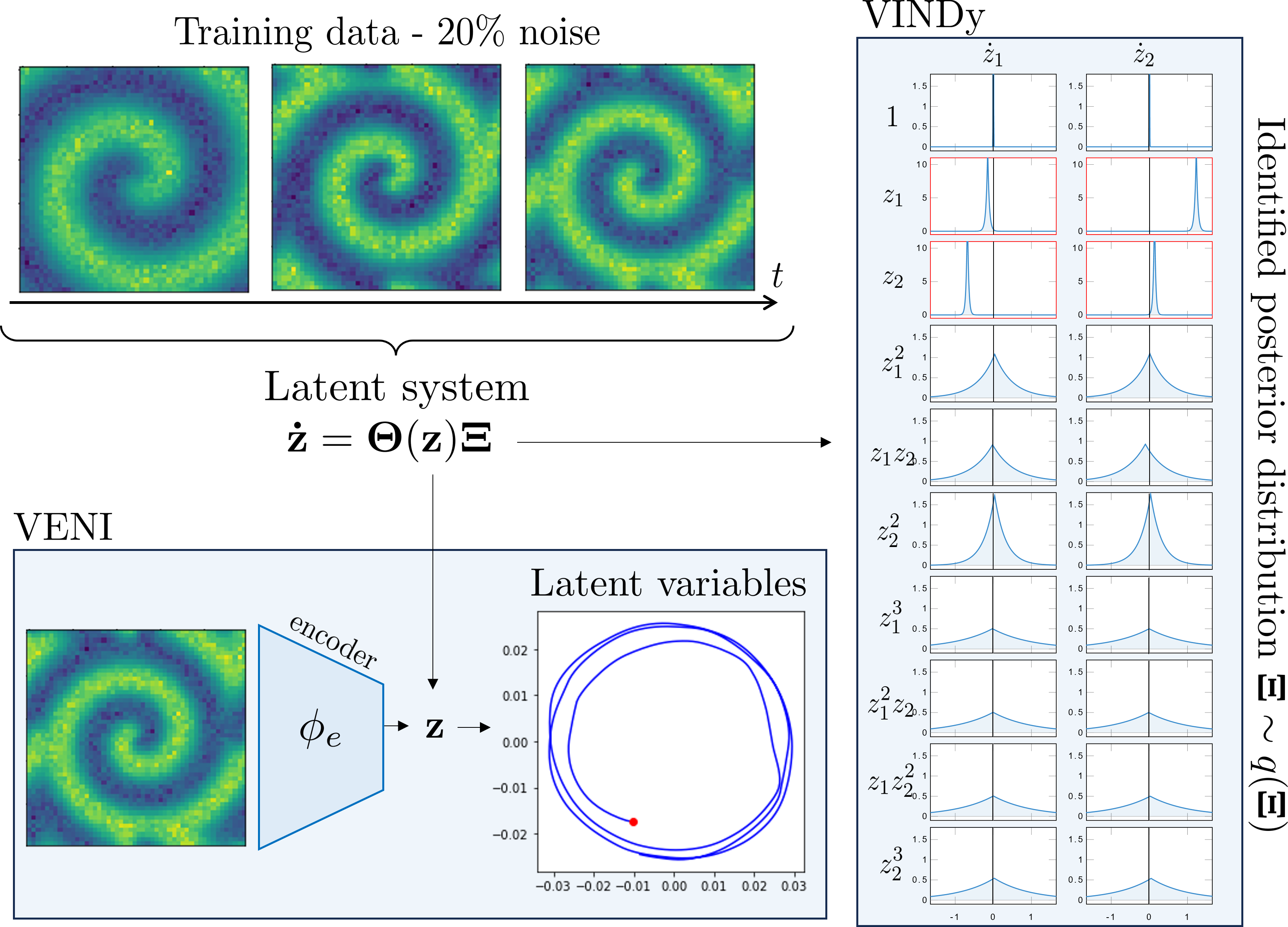
Figure 6: Results of the offline training, consisting of the VENI and VINDy steps, for the reaction-diffusion problem. In the VINDy box, we display the identified posterior distributions of the coefficients for the latent dynamic system. The rows represent the candidate terms considered for the dynamics, and the columns indicate which latent dynamic equation they belong to. We note that the mixed linear terms, which are the dominant terms for the observed dynamics, are accurately identified as significant. Most nonlinear terms contribute a mean of zero, and we observe that the uncertainty of the coefficients increases with the degree of the polynomial. In the VENI box, we highlight how the method is capable of learning an encoding function from noisy data, resulting in two latent variables that exhibit the expected oscillatory behavior.

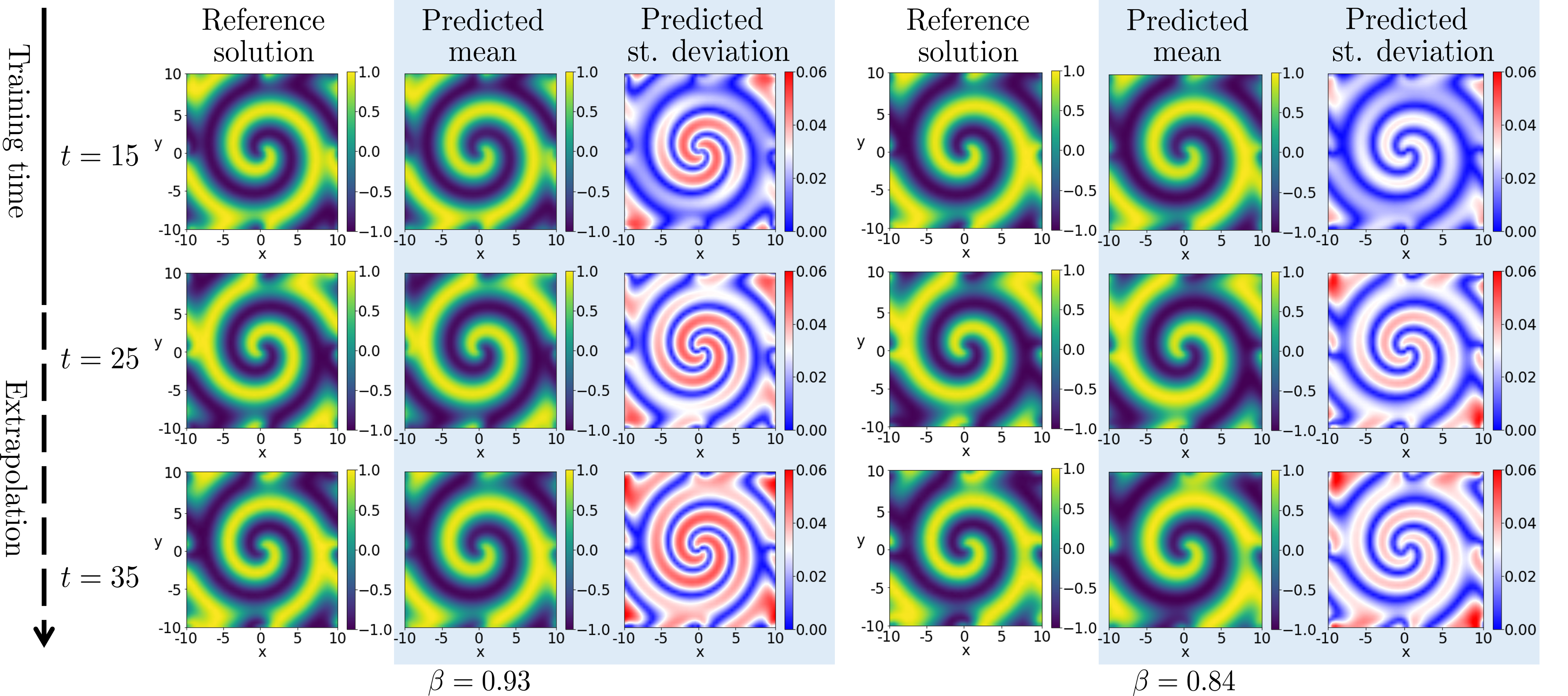
Figure 7: Comparison of solution fields in the reaction-diffusion example between the approximation by the proposed method and the numerical reference solution truth. The snapshots refer to one training time instances $t=15$ and two extrapolated time instances $t\in\{25,35\}$ (being $T_{\text{train}}=20$) for two testing parameter $\beta=\{0.93,0.84\}$. We report the prdictions of the mean and standard deviation of the solutions predicted by the VICI procedure.

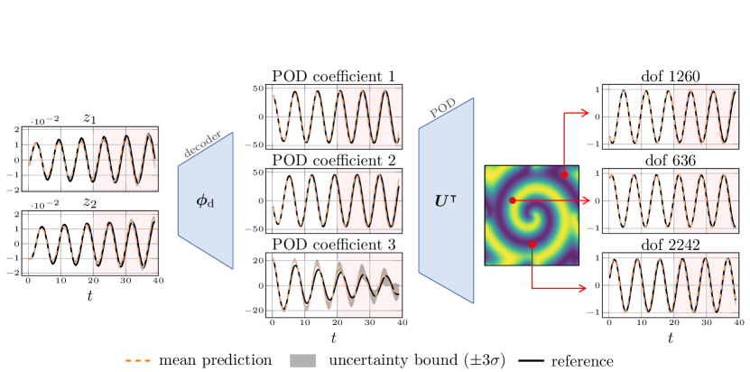
Figure 8: Forward uncertainty quantification at the different reduction levels, performed with the VICI procedure. The dashed line at $T_{\text{train}}=20$ indicates the end time of training data coverage. The red line indicates the noise-free reference solution, the dashed blue line the predicted mean, and the shaded region indicates the uncertainty bounds.

3.3 Numerical example III: Beam MEMS resonator

We consider a straight beam MEMS resonator, excited at resonance, which could be represented as double clamped beam. The illustration and the properties of the device are reported in Fig. 9.

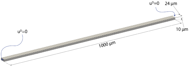
Figure 9: Schematic representation of the beam MEMS resonator with the mesh used in the FOM simulations. The beam has length $L=~{}1000$ $\mu$m with a rectangular cross-section of dimensions 10 $\mu$m $\times$24 $\mu$m , made of isotropic polysilicon [43], with density $\rho=~{}2330$ Kg/m³, Young modulus $E=167$ GPa and Poisson coefficient $\nu=0.22$. The first bending eigenfrequency is $\omega_{0}=0.5475\,\text{rad}/\mu\text{s}$. Dirichlet boundaries are highlighted.

The governing PDEs for this solid mechanics problem in large transformations [44] are formulated in terms of the displacement field $\mathbf{u}$ as follows:

$$\rho_{0}\ddot{\mathbf{u}}({\varkappa},t)-\nabla\cdot\mathbf{P}(\varkappa,t)-\rho_{0}\mathbf{B}(\varkappa,t;\bm{\beta})=\mathbf{0},\; \quad(\varkappa,t)\in\Omega_{0}\times(0,T),$$ (21a)

$$\mathbf{P}(\varkappa,t)\cdot\mathbf{N}(\varkappa)=\mathbf{0},\; \quad(\varkappa,t)\in\partial\Omega_{N}\times(0,T),$$ (21b)

$$\mathbf{u}(\varkappa,t)=\mathbf{0},\; \quad(\varkappa,t)\in\partial\Omega_{D}\times(0,T),$$ (21c)

where $\Omega_{0}$ is the domain occupied by the device in the undeformed configuration, described by material coordinates $\varkappa$, and $T=1755\,\mu\text{s}$.Eq. (21a) expresses the conservation of momentum where $\rho_{0}$ is the initial density, $\mathbf{P}$ is the first Piola-Kirchhoff stress and $\mathbf{B}$ are the external body forces. In this application we consider a periodic body load proportional to the first vibrational eigenfunction, with amplitude and frequency given by the parameters $F$ and $\omega$, respectively. The input parameter vector hence becomes $\bm{\beta}=[\omega,F]$, defined over a closed and bounded set of dimension 2. Eq. (21b) and (21c) define the homogeneous boundary conditions on the Neumann and Dirichlet and boundaries denoted as $\partial\Omega_{N}$ and $\partial\Omega_{D}$, respectively, and where $\mathbf{N}$ denotes the outward-directed unit normal on the boundary of $\Omega$. For more details regarding the application, we refer to [19].

Dataset

We consider $N_{\beta}=56$ parameter instances, corresponding to 28 values for the frequency $\omega$, selected in the range $[0.526,0.564]\,\text{rad}/\mu\text{s}$ with a finer sampling around the natural frequency $\omega_{0}$, and for two values of the forcing amplitude $F\in\{0.125,0.250\}\,\mu\text{N}$. In total, $N_{\beta}^{\text{train}}=28$ parameter instances are randomly selected to construct the training set and the remaining $N_{\beta}^{\text{test}}=28$ are retained for testing. Numerical solutions for the displacement are computed for each parameter configuration, by discretizing the system (21) using the finite element method over a spatial mesh consisting of $N_{\text{dof}}=7821$ degrees of freedom and using finite element method as in [19] of which only 5964 are nonzero. As we are modeling the beam as a second-order system, we require to have access or compute the second time derivatives $\ddot{\bm{x}}$ for training in addition to the system states $\bm{x}$ and their time derivatives $\dot{\bm{x}}$.

Training data are calculated up to $T_{\text{train}}=1091\,{\mu}s<T$ and corrupted by additive noise following a normal distribution which scale is proportional to the mean level of displacements over all training simulations. This step is particularly challenging for second-order systems where even low noise increases dramatically on the acceleration level as it grows with each numerical derivation, as showcased for the beam in Fig. 10 where the noisy training data is compared to noise-free reference data. For the beam data, the ratio between the maximum amplitude occurring in the noisy training data and the noise-free reference data on acceleration level across all simulations is $\numprint{4.52455}\pm\numprint{2.26626}$.

Figure 10: Noise-free and noisy trajectories of the y-displacement, velocity, and acceleration for a node in the middle of the beam for a example training simulation. For training only the first 1091$\,\mu$s of the noisy data are used; the remaining time for which the model extrapolates has red background.

As in the previous example, the data (including displacements, velocities, and accelerations) are preliminary projected onto a POD basis of $N=N_{\text{POD}}=3$ modes (extracted from the noisy displacement training data). Finally, snapshots of the displacement are collected in $\tilde{\mathbf{X}}_{\text{train}}\in\mathbb{R}^{N_{t}^{\text{train}}N_{\beta}^{\text{train}}\times N}$ and $\tilde{\mathbf{X}}_{\text{test}}\in\mathbb{R}^{N_{t}^{\text{train}}N_{\beta}^{\text{train}}\times N}$ matrices, where $N_{t}^{\text{train}}=14001$ and $N_{t}^{\text{test}}=22499$ are the corresponding numbers of time instances. Analogously, velocities are collected in $\dot{\tilde{\mathbf{X}}}_{\text{train}}$ and accelerations in $\ddot{\tilde{\mathbf{X}}}_{\text{train}}$.

Model

The encoder is composed of three hidden layers using 32 neurons each. The decoder has symmetrical structure. Although the dynamics of this system lies on a two dimensional manifold in the phase space, we manage to reduce the dimensionality to a single latent variable $n=1$, as the dependence on the velocity is the minimal for the master bending mode that we inspect herein. As in (21), structural mechanics problems are often governed by second-order governing equations. Therefore we model the reduced dynamics with a second-order ODE, by augmenting the reduce states with the first derivatives $\dot{z}$:

$$\frac{\text{d}}{\text{dt}}\begin{bmatrix}\;z\;\\ \;\dot{z}\;\end{bmatrix}=\mathbf{f}\left(z,\dot{z};\bm{\beta}\right)\approx\begin{bmatrix}\;\dot{z}\;\\ \;\bm{\Theta}(z,\dot{z};\bm{\beta})\bm{\Xi}\;\end{bmatrix}.$$ (22)

The corresponding accelerations at latent level $\ddot{\bm{z}}$ can be derived using chain rule as it is done for the velocities $\dot{\bm{z}}$.

Note that, in case we did not want to exploit any prior knowledge on the second-order structure of the problem, we could have equivalently modelled the problem by considering $n=2$ latent variables and identifying a first-order ODE system as in the previous example. The library $\bm{\Theta}$ features polynomials up to the third degree with respect to both $\bm{z}$ and $\dot{\bm{z}}$. Moreover, since the beam resonator is forced harmonically with amplitude and frequency parameterized by $F$ and $\omega$, we incorporate the parameter dependency by including the library term $F\cos(\omega t)$. We set gaussian priors on the reduced states $[\bm{z},\dot{\bm{z}}]^{\top}\sim\mathcal{N}(\mathbf{0},\bm{I})$ and laplacian prior on each of the VINDy coefficient distributions $\bm{\Xi}_{ij}\sim\mathcal{L}(0,1)$. Training is performed for 2500 epochs, and the weights of the networks that performed best in terms of total loss on a validation subset of the training data used for inference. After training we apply PDF zero tresholding, see Section 2.5.1, to only keep the terms that are important to describe the dynamics. In particular, all terms with a $pdf_{\bm{\Xi}_{ij}}(0)>1.9$ are neglected in the model.

3.3.1 Results

The clamped-clamped beam is a classical structure showing Duffing-like hardening behavior [45, 46] that can be accurately described by the following simple model:

$$\ddot{z}=-\omega_{0}^{2}z-2\xi\omega_{0}\dot{z}-\gamma z^{3}-\alpha F\cos(\omega t),$$ (23)

where the cubic term, with $\gamma>0$, accounts for the hardening response and the absence of quadratic terms should be remarked. As the objective of VINDy is to identify a sparse reduced system, we wish to unveil the normal form underlying the observed high-dimensional system, directly from data. For the considered example, we can see from Fig. 11 that the terms indicated as relevant by our proposed method correspond to the ones present in the normal form (23) plus an additional bias term of small magnitude. Moreover the actual coefficients $\omega_{0}$ and $\xi$ could be retrieved from the spectral properties of the linearization of system (21). These coefficients represent the natural frequency and the damping of the device, respectively, and uniquely determine the linear terms in the reduced dynamics. In the considered problem, $\omega_{0}=0.5475\,\text{rad}/\mu\text{s}$ and $\xi=0.01\,{\mu\text{s}}^{-1}$. Our method successfully manages to accurately identify the linear terms $-\omega_{0}^{2}$ and $2\xi\omega_{0}$ (see Fig.11), from noisy data, without accessing or incorporating knowledge from the full order model.

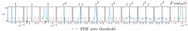
Figure 11: Beam coefficient distribution. The terms that appear in the normal form of the observed high-dimensional system are framed in red. The cutoff value that determines which terms are kept is shown as dashed line. Moreover, the correct values that result from the natural frequency and the damping of the system are marked with a black triangle at the bottom of the according axis.

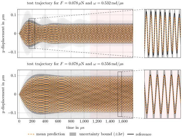
Figure 12: Physical reconstruction of latent mean trajectories and corresponding uncertainties for a node in the middle of the beam where the most dynamics occur for two example test simulations. For training only the first $T_{\text{train}}=1091\,\mu$s are used; the remaining time for which the model extrapolates has a red background.

Finally, we demonstrate the performance of the proposed method to generate the full-time evolution of the observed system for new parameter configurations following the VICI procedure. In Fig. 12, we illustrate that the reconstruction of the integrated latent dynamics accurately follows the reference. The trajectory resulting from the means of the coefficient distribution closely aligns with the actual course and the standard deviations resulting from the VICI approach cover the discrepancy throughout the trajectories.

To get a better visualization of the performance over the entire beam, we present in Fig. 13 a complete representation of the deformed beam at different points in time showing a contour plot of displacement errors. Clearly recognisable, the prediction follows the reference solution satisfactorily over the time period considered (including extrapolation in time).

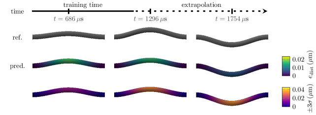
Figure 13: Example simulation of the beam at three time instants. The reference solution is shown at the top, whereas a physical reconstruction of the integrated latent dynamics is shown below. For the latter, we once colorize it with respect to the Euclidean distance $e_{\text{disp}}$ between the nodes of the FE beam in the reference simulation and their predicted positions as displacement error, and once with the corresponding uncertainty bounds resulting from the VICI framework. The beam is shrunk to 20% of its length for better visualization and the displacements are scaled by a factor of 100 for the same reason. Across all test simulations, our approach achieves an average normalised displacement error of $\numprint{0.06350993813174313}\pm\numprint{0.03068206826380863}$ using the mean trajectories. For this performance quantity, the average node displacement error of all nodes and time instances is normalised by the maximum displacement occurring in the respective simulation.

4 Discussion and concluding remarks

The paper introduces a novel framework – named VENI, VINDy, VICI – for creating interpretable, generative reduced-order models that can simulate high-dimensional, nonlinear dynamical systems with embedded uncertainty quantification. The proposed method efficiently provides accurate and reliable estimates by combining variational autoencoders with a newly introduced variational identification of nonlinear dynamics (VINDy) technique. VINDy identifies an interpretable, probabilistic model for the reduced dynamics by learning the distribution of coefficients of the linear combination of a parsimonious set of functions selected from a library of candidates.
As a result, in a purely data-driven and automated fashion, our overall method simultaneously learns the probability distribution of low-dimensional representation of the system states together with a probabilistic dynamical model, describing how the states evolve in time. Moreover, by adeptly accounting for uncertainty during both training and testing phases, the method operates effectively in high-noise and low-data regimes, and provides uncertainty-aware predictions for varying parameter configurations and initial conditions of the system.

The method’s effectiveness is showcased across various benchmarks, including the low-dimensional Rössler system to assess handling different sources and intensities of uncertainty, and high-dimensional PDE problems in fluid dynamics with a parametrised reaction-diffusion problem, and in structural mechanics with the hardening behavior of a micro electro-mechanical resonator.

A key feature of the method is the usage of variational inference to reformulate UQ as an optimization problem, solvable with efficient gradient-based techniques. This significantly reduces computational costs with respect to alternative strategies based on Bayesian or Monte Carlo methods. Moreover, it allows to seamlessly integrate UQ with the learning tasks into a single, training procedure.

As drawback, as with most deep learning frameworks, the proposed method can be sensitive to the weights initialization, choice of the priors and hyperparameters, such as, e.g., the weighting coefficients leveraging the contribution of the different loss terms in (17). In Sect. 2.4 we provided a general guidance on how to set these hyperparameters, but automatic, and more sophisticated hyperparameter-tuning techniques or constrained learning could complement the current framework.

A further improvement could be achieved by considering more advanced neural network models as building block of the variational autoencoders. For instance, graph neural networks [47] are more expressive in reconstructing spatial pattern so they can substitute the feed-forward neural networks. Indeed, while the method showcases accurate forecast of dynamics and extrapolation with respect to time thanks to the identified, explicit dynamical model, we do not expect as good generalization capabilities from feed-forward networks in predicting spatial patterns that are totally unseen over the training.

Finally we observe that, while UQ on the dynamical model could be inferred directly from the identified posterior distributions of the model coefficients, performing UQ over the predicted time trajectories, instead requires a sampling strategy, ı.e. VICI. Indeed, the reduced states are treated as independent and identically distributed (iid) variables, making them completely agnostic of time. So UQ over trajectories is computed by VICI from the statistical moments of different integrated trajectories from different realizations of initial conditions and coefficients of the dynamical model. Further developments could model latent states as random processes, thus accounting for time dependence and providing more rigorous UQ for the predicted trajectories.

The non-intrusive, data-driven nature of the framework requires minimal a priori knowledge of the observed system and could handle model and measurement noise. This paves the way for applications to real-life datasets, potentially considering various data types, such as those coming from sensors or videos as in [27, 7]. As further direction of future work, the flexibility and generality of the framework offers promising prospects for its extension to online learning within the context of digital twins, enabling dynamic model updates as new data emerge. This could be done by adopting previous posterior estimates as priors and fine-tuning the model to refine posterior distributions.

Appendix A Appendix

A.1 VINDy Loss

In this section we derive equation (13) in Section 2.2. We assume that $\bm{\Xi}$ and $\bm{z}$ are independent. This reflects the fact that $\bm{\Xi}$ are constant coefficients determining the contribution of each candidate feature in the dynamics, thus they are related to the underlying physical model we aim to discover and not to the specific (latent) observed data.

In VINDy, we approximate the distribution of $p(\bm{\Xi}|\dot{\bm{z}})$ of $\bm{\Xi}|\dot{\bm{z}}$ with a posterior distribution $q(\bm{\Xi})$ parameterized by trainable weights. We aim to minimize the KL divergence between the approximated posterior and the true one:

$$\begin{split}\text{KL}(q(\bm{\Xi})\parallel p(\bm{\Xi}\mid\dot{\bm{z}}))&=\mathbb{E}_{\bm{\Xi}\sim q(\bm{\Xi})}[\log q(\bm{\Xi})]-\mathbb{E}_{\bm{\Xi}\sim q(\bm{\Xi})}[\log p(\bm{\Xi}\mid\dot{\bm{z}})]\\ &=\mathbb{E}_{\bm{\Xi}\sim q(\bm{\Xi})}[\log q(\bm{\Xi})]-\mathbb{E}_{\bm{\Xi}\sim q(\bm{\Xi})}[\log p(\bm{\Xi}\mid\dot{\bm{z}},\,\bm{z})]\\ &=\mathbb{E}_{\bm{\Xi}\sim q(\bm{\Xi})}[\log q(\bm{\Xi})]-\mathbb{E}_{\bm{\Xi}\sim q(\bm{\Xi})}\left[\log\frac{{p(\bm{\Xi},\,\bm{z})}p(\dot{\bm{z}}\mid\bm{\Xi},\,\bm{z})}{p(\dot{\bm{z}}\mid{\bm{z}})p({\bm{z}})}\right]\\ &=\mathbb{E}_{\bm{\Xi}\sim q(\bm{\Xi})}[\log q(\bm{\Xi})]-\mathbb{E}_{\bm{\Xi}\sim q(\bm{\Xi})}\left[\log\frac{p(\bm{\Xi})p(\bm{z})p(\dot{\bm{z}}\mid\bm{\Xi},\,\bm{z})}{p(\dot{\bm{z}}\mid{\bm{z}})p({\bm{z}})}\right]\\ &=\mathbb{E}_{\bm{\Xi}\sim q(\bm{\Xi})}[\log q(\bm{\Xi})]-\mathbb{E}_{\bm{\Xi}\sim q(\bm{\Xi})}\left[\log p(\bm{\Xi})\right]-\mathbb{E}_{\bm{\Xi}\sim q(\bm{\Xi})}\left[\log(p(\dot{\bm{z}}\mid\bm{\Xi},\,\bm{z}))\right]+\log p(\dot{\bm{z}}\mid{\bm{z}})\\ &=\text{KL}(q(\bm{\Xi})\parallel p(\bm{\Xi}))-\mathbb{E}_{\bm{\Xi}\sim q(\bm{\Xi})}\left[\log(p(\dot{\bm{z}}\mid\bm{\Xi},\,\bm{z}))\right]+\log p(\dot{\bm{z}}\mid{\bm{z}}).\end{split}$$ (24)

The resulting expression has been obtained by applying KL divergence definition, Bayes’ theorem on the second term and exploiting the independence between $\bm{\Xi}$ and $\bm{z}$.
Analogously, the KL divergence between $p(\bm{z}|\dot{\bm{z}})$ and its approximation by means of the posterior $q(\bm{z})$ can be written as

$$\begin{split}\text{KL}(q(\bm{z})\parallel p(\bm{z}\mid\dot{\bm{z}}))&=\mathbb{E}_{\bm{z}\sim q(\bm{z})}[\log q(\bm{z})]-\mathbb{E}_{\bm{z}\sim q(\bm{z})}[\log p(\bm{z}\mid\dot{\bm{z}})]\\ &=\mathbb{E}_{\bm{z}\sim q(\bm{z})}[\log q(\bm{z})]-\mathbb{E}_{\bm{z}\sim q(\bm{z})}[\log p(\bm{z})]-\mathbb{E}_{\bm{z}\sim q(\bm{z})}[\log p(\dot{\bm{z}}\mid\bm{z})]+\log p(\dot{\bm{z}})\\ &=\text{KL}(q(\bm{z})\parallel p(\bm{z}))-\mathbb{E}_{\bm{z}\sim q(\bm{z})}[\log p(\dot{\bm{z}}\mid\bm{z})]+\log p(\dot{\bm{z}}).\end{split}$$ (25)

Summing them up leads to

$$\begin{split}\text{KL}(q(\bm{\Xi})\parallel p(\bm{\Xi}\mid\dot{\bm{z}}))+&\text{KL}(q(\bm{z})\parallel p(\bm{z}\mid\dot{\bm{z}}))\\ =&\,\text{KL}(q(\bm{\Xi})\parallel p(\bm{\Xi}))-\mathbb{E}_{\bm{\Xi}\sim q(\bm{\Xi})}\left[\log(p(\dot{\bm{z}}\mid\bm{\Xi},\,\bm{z}))\right]+\log p(\dot{\bm{z}}\mid{\bm{z}})\,+\\ &\,\text{KL}(q(\bm{z})\parallel p(\bm{z}))-\mathbb{E}_{\bm{z}\sim q(\bm{z})}[\log p(\dot{\bm{z}}\mid\bm{z})]+\log p(\dot{\bm{z}})\\ =&\,\text{KL}(q(\bm{\Xi})\parallel p(\bm{\Xi}))+\text{KL}(q(\bm{z})\parallel p(\bm{z}))-\mathbb{E}_{\bm{\Xi}\sim q(\bm{\Xi})}\left[\log(p(\dot{\bm{z}}\mid\bm{\Xi},\,\bm{z}))\right]+\log p(\dot{\bm{z}}).\end{split}$$ (26)

The last equality follows from the standard assumption of stochastic gradient descent-based methods: at each optimization step, we take a sample of $\bm{z}$ and treat $\log p(\dot{\bm{z}}|\bm{z})$ as an approximation of $\mathbb{E}_{\bm{z}\sim q(\bm{z})}[\log p(\dot{\bm{z}}|\bm{z})]$, thus assuming $\log p(\dot{\bm{z}}|\bm{z})-\mathbb{E}_{\bm{z}\sim q(\bm{z})}[\log p(\dot{\bm{z}}|\bm{z})]\approx 0$.
Finally, equation (26) can be rewritten as

$$\begin{split}\log p(\dot{\bm{z}})&-\text{KL}(q(\bm{\Xi})\parallel p(\bm{\Xi}|\dot{\bm{z}}))-\text{KL}(q(\bm{z})\parallel p(\bm{z}|\dot{\bm{z}}))=\\ &=\mathbb{E}_{\bm{\Xi}\sim q(\bm{\Xi})}\left[\log(p(\dot{\bm{z}}\mid\bm{\Xi},\bm{z}))\right]-\text{KL}(q(\bm{\Xi})\parallel p(\bm{\Xi}))-\text{KL}(q(\bm{z})\parallel p(\bm{z})),\end{split}$$

that is exactly the VINDy objective function in (13).

A.2 Prior Distributions

The priors $p(\bm{\Xi})$ and $p(\bm{z})$ in the context of VENI and VINDy can be used to infuse knowledge about the distributions of the coefficients of the dynamics and latent states. If no prior knowledge about the distribution’s shape and its parameters is present, Gaussian priors are a common choice in variational inference, especially in VAEs. Moreover, using latent Gaussian distributions for the latent variables allows modeling arbitrarily complex output distributions if the decoder is sufficiently complex [48]. A valid alternative, especially when model the dynamics’ coefficients is the use of Laplacian priors. In contrast to Gaussian priors, Laplacian priors can act as sparsity-promoting regularization terms within a regression task [26]. Consequently, they are more prone to provide a parsimonious dynamical model, which is in general highly desirable [49]. We furthermore want highlight that adjusting the priors are an elegant way of incorporating any existing pre-knowledge about occurring function terms. Other possible choices for the priors may include spike and slab, regularized horseshoe, etc. In this work, we focus on Gaussian and Laplacian priors, since they have the additional advantage that the KL divergence between two distribution of the same family can be expressed in a closed-form, as presented in the following.

Gaussian

The Gaussian distribution

$$\mathcal{N}({\mu}^{\mathcal{N}},{{\delta}^{\mathcal{N}}})$$ (27)

is parameterized by its mean ${\mu}^{\mathcal{N}}$ and variance ${{\delta}^{\mathcal{N}}}$. For two univariate Gaussian distributions the KL divergence can be calculated using the closed form

$$\text{KL}(\mathcal{N}({\mu}^{\mathcal{N}}_{1},{\delta}^{\mathcal{N}}_{1})\parallel\mathcal{N}({\mu}^{\mathcal{N}}_{2},{\delta}^{\mathcal{N}}_{2}))=\log(\frac{{\delta}^{\mathcal{N}}_{2}}{{\delta}^{\mathcal{N}}_{1}})+\frac{{{\delta}^{\mathcal{N}}_{1}}^{2}+({\mu}^{\mathcal{N}}_{2}-{\mu}^{\mathcal{N}}_{1})^{2}}{2{{\delta}^{\mathcal{N}}_{2}}^{2}}-\frac{1}{2}.$$ (28)

Laplace

A Laplace distribution

$$\mathcal{L}({\mu}^{\mathcal{L}},{\delta}^{\mathcal{L}})$$ (29)

is parameterized by a location ${\mu}^{\mathcal{L}}$ and a scale parameter ${\delta}^{\mathcal{L}}$. For gradient-based optimization the reparameterization trick for a Laplace distribution looks similar as the one for Gaussian ones

$$\bm{z}={\mu}^{\mathcal{L}}+\bm{\zeta}{\delta}^{\mathcal{L}},\quad\bm{\zeta}\sim\mathcal{L}(0,1).$$ (30)

Given two Laplace distributions, the KL divergence can be calculated in closed form as

$$\text{KL}(\mathcal{L}({\mu}^{\mathcal{L}}_{1},{\delta}^{\mathcal{L}}_{1})\parallel\mathcal{L}({\mu}^{\mathcal{L}}_{2},{\delta}^{\mathcal{L}}_{2}))=\log(\frac{{\delta}^{\mathcal{L}}_{2}}{{\delta}^{\mathcal{L}}_{1}})+\frac{{\delta}^{\mathcal{L}}_{1}\exp{-\frac{|{\mu}^{\mathcal{L}}_{1}-{\mu}^{\mathcal{L}}_{2}|}{{\delta}^{\mathcal{L}}_{1}}}+|{\mu}^{\mathcal{L}}_{1}-{\mu}^{\mathcal{L}}_{2}|}{{\delta}^{\mathcal{L}}_{2}}-1,$$ (31)

see [50].

References

- [1] T. Bui-Thanh, K. Willcox, O. Ghattas, Parametric reduced-order models for probabilistic analysis of unsteady aerodynamic applications, AIAA journal 46 (10) (2008) 2520–2529.
- [2] A. Manzoni, A. Quarteroni, G. Rozza, Shape optimization for viscous flows by reduced basis methods and free-form deformation, International Journal for Numerical Methods in Fluids 70 (5) (2012) 646–670. doi:10.1002/fld.2712.
- [3] J. S. Hesthaven, G. Rozza, B. Stamm, Certified reduced basis methods for parametrized partial differential equations, Springer International Publishing, 2016.
- [4] A. Quarteroni, A. Manzoni, F. Negri, Reduced Basis Methods for Partial Differential Equations. An Introduction, Springer International Publishing, 2016.
- [5] P. Benner, S. Gugercin, K. Willcox, A survey of projection-based model reduction methods for parametric dynamical systems, SIAM review 57 (4) (2015) 483–531. doi:10.1137/130932715.
- [6] C. Fefferman, S. Mitter, H. Narayanan, Testing the manifold hypothesis, Journal of the American Mathematical Society 29 (4) (2016) 983–1049. doi:10.1090/jams/852.
- [7] B. Chen, K. Huang, S. Raghupathi, I. Chandratreya, Q. Du, H. Lipson, Automated discovery of fundamental variables hidden in experimental data, Nature Computational Science 2 (7) (2022) 433–442. doi:10.1038/s43588-022-00281-6.
- [8] S. L. Brunton, J. L. Proctor, J. N. Kutz, Discovering governing equations from data by sparse identification of nonlinear dynamical systems, Proceedings of the national academy of sciences 113 (15) (2016) 3932–3937. doi:10.1073/pnas.1517384113.
- [9] J. Bongard, H. Lipson, Automated reverse engineering of nonlinear dynamical systems, Proceedings of the National Academy of Sciences 104 (24) (2007) 9943–9948. doi:10.1073/pnas.0609476104.
- [10] M. Schmidt, H. Lipson, Distilling free-form natural laws from experimental data, Science 324 (5923) (2009) 81–85. doi:10.1126/science.1165893.
- [11] O. Yair, R. Talmon, R. R. Coifman, I. G. Kevrekidis, Reconstruction of normal forms by learning informed observation geometries from data, Proceedings of the National Academy of Sciences 114 (38) (2017) E7865–E7874. doi:10.1073/pnas.1620045114.
- [12] K. Duraisamy, G. Iaccarino, H. Xiao, Turbulence modeling in the age of data, Annual review of fluid mechanics 51 (2019) 357–377. doi:10.1146/annurev-fluid-010518-040547.
- [13] M. Quade, M. Abel, K. Shafi, R. K. Niven, B. R. Noack, Prediction of dynamical systems by symbolic regression, Physical Review E 94 (1) (2016) 012214.
- [14] L. Rosafalco, P. Conti, A. Manzoni, S. Mariani, A. Frangi, Ekf-sindy: Empowering the extended kalman filter with sparse identification of nonlinear dynamics, arXiv preprint arXiv:2404.07536 (2024).
-
[15]
M. Raissi, G. E. Karniadakis, Hidden physics models: Machine learning of nonlinear partial differential equations, J. Comput. Phys. 357 (2017) 125–141.
doi:10.1016/j.jcp.2017.11.039.
URL https://api.semanticscholar.org/CorpusID:2680772 - [16] B. Lusch, J. N. Kutz, S. L. Brunton, Deep learning for universal linear embeddings of nonlinear dynamics, Nature communications 9 (1) (2018) 1–10. doi:10.1038/s41467-018-07210-0.
- [17] K. Champion, B. Lusch, J. N. Kutz, S. L. Brunton, Data-driven discovery of coordinates and governing equations, Proceedings of the National Academy of Sciences 116 (45) (2019) 22445–22451. doi:10.1073/pnas.1906995116.
- [18] J. Bakarji, K. Champion, J. Nathan Kutz, S. L. Brunton, Discovering governing equations from partial measurements with deep delay autoencoders, Proceedings of the Royal Society A 479 (2276) (2023) 20230422. doi:10.1038/s41467-018-07210-0.
- [19] P. Conti, G. Gobat, S. Fresca, A. Manzoni, A. Frangi, Reduced order modeling of parametrized systems through autoencoders and SINDy approach: continuation of periodic solutions, Computer Methods in Applied Mechanics and Engineering 411 (2023) 116072. doi:10.1016/j.cma.2023.116072.
- [20] D. P. Kingma, M. Welling, Auto-encoding variational bayes, arXiv preprint (Dec. 2013). arXiv:1312.6114, doi:10.48550/arXiv.1312.6114.
- [21] I. Higgins, D. Amos, D. Pfau, S. Racaniere, L. Matthey, D. Rezende, A. Lerchner, Towards a definition of disentangled representations, arXiv preprint arXiv:1812.02230 (2018). doi:10.48550/arXiv.1812.02230.
- [22] A. A. Alemi, I. Fischer, J. V. Dillon, K. Murphy, Deep variational information bottleneck, arXiv preprint arXiv:1612.00410 (2016). doi:10.48550/arXiv.1612.00410.
- [23] A. Solera-Rico, C. Sanmiguel Vila, M. Gómez-López, Y. Wang, A. Almashjary, S. T. Dawson, R. Vinuesa, -variational autoencoders and transformers for reduced-order modelling of fluid flows, Nature Communications 15 (1) (2024) 1361. doi:10.48550/arXiv.1812.02230.
- [24] T. Simpson, K. Vlachas, A. Garland, N. Dervilis, E. Chatzi, Vprom: a novel variational autoencoder-boosted reduced order model for the treatment of parametric dependencies in nonlinear systems, Scientific Reports 14 (1) (2024) 6091. doi:10.1038/s41467-024-45578-4.
- [25] N. Botteghi, M. Guo, C. Brune, Deep kernel learning of dynamical models from high-dimensional noisy data, Scientific reports 12 (1) (2022) 21530. doi:10.1038/s41598-022-25362-4.
-
[26]
S. M. Hirsh, D. A. Barajas-Solano, J. N. Kutz, Sparsifying priors for bayesian uncertainty quantification in model discovery, Royal Society Open Science 9 (2) (2022) 211823.
arXiv:https://royalsocietypublishing.org/doi/pdf/10.1098/rsos.211823, doi:10.1098/rsos.211823.
URL https://royalsocietypublishing.org/doi/abs/10.1098/rsos.211823 - [27] L. Mars Gao, J. Nathan Kutz, Bayesian autoencoders for data-driven discovery of coordinates, governing equations and fundamental constants, Proceedings of the Royal Society A 480 (2286) (2024) 20230506. doi:10.1098/rspa.2023.0506.
- [28] R. K. Niven, L. Cordier, A. Mohammad-Djafari, M. Abel, M. Quade, Dynamical system identification, model selection and model uncertainty quantification by bayesian inference (2024). doi:10.48550/ARXIV.2401.16943.
- [29] D. A. Messenger, D. M. Bortz, Weak sindy for partial differential equations, Journal of Computational Physics 443 (2021) 110525.
-
[30]
Z. Wang, X. Huan, K. Garikipati, Variational system identification of the partial differential equations governing the physics of pattern-formation: Inference under varying fidelity and noise, Computer Methods in Applied Mechanics and Engineering 356 (2019) 44–74.
doi:https://doi.org/10.1016/j.cma.2019.07.007.
URL https://www.sciencedirect.com/science/article/pii/S0045782519304037 - [31] M. Jacobs, B. W. Brunton, S. L. Brunton, J. N. Kutz, R. V. Raut, Hypersindy: Deep generative modeling of nonlinear stochastic governing equations (2023). arXiv:2310.04832.
- [32] K. Course, P. B. Nair, State estimation of a physical system with unknown governing equations, Nature 622 (7982) (2023) 261–267. doi:10.1038/s41586-023-06574-8.
- [33] L. Mars Gao, J. Nathan Kutz, Bayesian autoencoders for data-driven discovery of coordinates, governing equations and fundamental constants, Proceedings of the Royal Society A 480 (2286) (2024) 20230506.
- [34] R. Yu, A tutorial on vaes: From bayes’ rule to lossless compression (2020). arXiv:2006.10273.
-
[35]
M. Abdar, F. Pourpanah, S. Hussain, D. Rezazadegan, L. Liu, M. Ghavamzadeh, P. Fieguth, X. Cao, A. Khosravi, U. R. Acharya, V. Makarenkov, S. Nahavandi, A review of uncertainty quantification in deep learning: Techniques, applications and challenges, Information Fusion 76 (2021) 243–297.
doi:https://doi.org/10.1016/j.inffus.2021.05.008.
URL https://www.sciencedirect.com/science/article/pii/S1566253521001081 - [36] K. Gundersen, A. Oleynik, N. Blaser, G. Alendal, Semi-conditional variational auto-encoder for flow reconstruction and uncertainty quantification from limited observations, Physics of Fluids 33 (1) (Jan. 2021). doi:10.1063/5.0025779.
- [37] D. P. Kingma, J. Ba, Adam: A method for stochastic optimization, arXiv abs/1412.6980 (2014).
-
[38]
D. J. Rezende, S. Mohamed, D. Wierstra, Stochastic backpropagation and approximate inference in deep generative models, in: E. P. Xing, T. Jebara (Eds.), Proceedings of the 31st International Conference on Machine Learning, Vol. 32 of Proceedings of Machine Learning Research, PMLR, Bejing, China, 2014, pp. 1278–1286.
URL https://proceedings.mlr.press/v32/rezende14.html -
[39]
I. Higgins, L. Matthey, A. Pal, C. Burgess, X. Glorot, M. Botvinick, S. Mohamed, A. Lerchner, beta-vae: Learning basic visual concepts with a constrained variational framework, in: International conference on learning representations, 2016.
URL https://openreview.net/forum?id=Sy2fzU9gl -
[40]
L. Chamon, A. Ribeiro, Probably approximately correct constrained learning, in: H. Larochelle, M. Ranzato, R. Hadsell, M. Balcan, H. Lin (Eds.), Advances in Neural Information Processing Systems, Vol. 33, Curran Associates, Inc., 2020, pp. 16722–16735.
URL https://proceedings.neurips.cc/paper_files/paper/2020/file/c291b01517f3e6797c774c306591cc32-Paper.pdf - [41] D. Floryan, M. D. Graham, Data-driven discovery of intrinsic dynamics, Nature Machine Intelligence (2022) 1–8doi:10.1038/s42256-022-00575-4.
- [42] L. N. Trefethen, Spectral methods in MATLAB, SIAM, 2000.
- [43] A. Corigliano, B. De Masi, A. Frangi, C. Comi, A. Villa, M. Marchi, Mechanical characterization of polysilicon through on-chip tensile tests, Journal of Microelectromechanical Systems 13 (2) (2004) 200–219.
- [44] L. E. Malvern, Introduction to the mechanics of a continuous medium, EPS, Prentice-Hall series in engineering of the physical sciences, Prentice-Hall, Englewood Cliffs, NJ, 1969, literaturangaben.
- [45] A. Corigliano, R. Ardito, C. Comi, A. Frangi, A. Ghisi, S. Mariani, Mechanics of microsystems, John Wiley & Sons, 2018.
- [46] A. Frangi, G. Gobat, Reduced order modelling of the non-linear stiffness in MEMS resonators, International Journal of Non-Linear Mechanics 116 (2019) 211 – 218.
- [47] J. Zhou, G. Cui, S. Hu, Z. Zhang, C. Yang, Z. Liu, L. Wang, C. Li, M. Sun, Graph neural networks: A review of methods and applications, AI open 1 (2020) 57–81.
- [48] L. Devroye, Sample-based non-uniform random variate generation, in: Proceedings of the 18th conference on Winter simulation, 1986, pp. 260–265.
- [49] J. N. Kutz, S. L. Brunton, Parsimony as the ultimate regularizer for physics-informed machine learning, Nonlinear Dynamics 107 (3) (2022) 1801–1817. doi:10.1007/s11071-021-07118-3.
- [50] G. P. Meyer, An alternative probabilistic interpretation of the huber loss, in: Proceedings of the IEEE/CVF Conference on Computer Vision and Pattern Recognition (CVPR), 2021, pp. 5261–5269.