Quantum Magnetic Skyrmions on the Kondo Lattice
Abstract
A quantum description is given of nanoskyrmions in 2D textures with localised spins and itinerant electrons, isolated or coupled to leads, in or out of equilibrium. The spin-electron exchange is treated at the mean-field level, while Tensor Networks and exact diagonalization or nonequilibrium Green’s functions are used for localised spins and itinerant electrons. We motivate our scheme via exact benchmarks, then show by several examples that itinerant electrons distinctly affect the properties of quantum nanoskyrmions. Finally, we mention lines of future work and improvement of the approach.
Magnetic skyrmions are topologically protected, long-lived spin textures which can be manipulated by ultralow currents [1, 2, 3, 4, 5, 6, 7, 8, 9, 10, 11], and of great potential for applications in spintronics and quantum computing [12, 13, 14, 15, 16]. Skyrmions originate from the interplay of different types of magnetic interactions in solids [17], such as Heisenberg exchange [18], Dzyaloshinskii-Moriya interaction (DMI) [19, 20], and anisotropy [21, 22], to mention some.
Theoretical descriptions of skyrmions often treat spins classically [23, 24, 25, 26], via the Landau-Lifshitz-Gilbert [27, 28] and Thiele equations [29]. While very successful, these formulations, where itinerant electrons (i-electrons) enter implicitly or as a source of renormalization of the classical spin dynamics, are not always adequate.
For example, a classical description of the spins is reliable for skyrmion sizes of hundreds of lattice constants and large spin (), where quantum fluctuations are small. However, as experiments motivate, for nanometer-scale skyrmions [23] (and, in general, for ) a quantum description [30, 31, 32, 33, 34] is in order. This is usually via exact diagonalization (ED) and Tensor Networks [35, 36, 37, 38] (for recent analytical and dynamical mean-field-theory studies, see [33, 34]).
Furthermore, describing explicitly the interaction (via Kondo exchange) of the i-electrons with the localised spins (l-spins) can also be important, to e.g. address interface phenomena like current-driving and optical generation of nanoskyrmions [39]. At the atomistic level, most i-electrons+l-spins schemes treat the spins classically and the electrons quantum mechanically [40, 41, 42, 43, 44, 45, 46, 47, 48]. Computations are then viable also for fairly large samples, but the outcome can be at variance with exact quantum results [49], obtained by ED or by mapping the (2D) spin-electron system to mixed chains to use the Density Matrix Renormalization Group (DMRG). Since both spins and electrons are explicitly treated, such exact results are from small clusters and mostly for benchmark uses.
Thus, it is highly desirable (in fact necessary in several cases) to have a framework including i-electrons and electronic reservoirs/leads, but not neglecting the quantum effects on nanoskyrmions. However, to proceed, approximations are needed, since in essence one deals with a Kondo-lattice problem, further complicated by Heisenberg and DMI interactions for the l-spins.
In this work, we propose a practically viable quantum treatment for both skyrmions and electrons, in- and out-of-equilibrium. The approach rests on a mean-field treatment of the Kondo-exchange. Yet, it describes at the quantum level both spin-texture and electron dynamics, to access intrinsically quantum physical quantities, e.g. spin-entanglement and quantum spin chirality. Furthermore, our numerical results for different system and situations illustrate the merit of the approach and show that including explicitly i-electrons has a very noticeable effect on the properties of quantum nanoskyrmions.
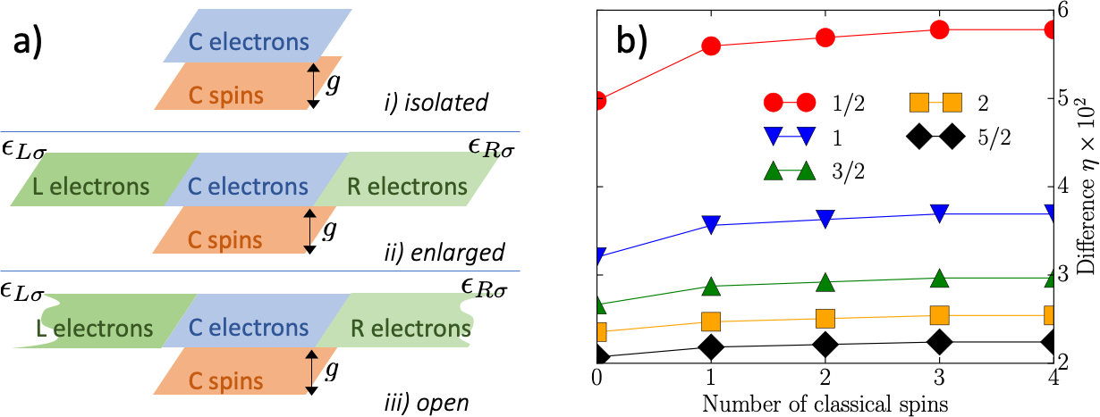
System and Hamiltonian. We consider three setups of increasing complexity, shown in Fig. 1a. By denoting as () the regions where the l-spins (i-electrons) reside, we have i) both l-spins and i-electrons in the same finite lattice ; ii) l-spins in , and i-electrons in an enlarged finite lattice , where region () is coupled to from the left (right); iii) same as ii), but with semi-infinite and regions. We describe i-iii) via a Kondo lattice Hamiltonian plus Heisenberg and DMI, i.e. with
| (1) |
Here, is the i-electrons part, with hopping parameter between nearest-neighbour (n.n.) sites, and creating an electron with spin projection at site . The l-spins texture is described by , where is the spin operator at site , and , , and respectively denote the Heisenberg exchange, a Neel-type DMI, and the external magnetic field. Finally, is the Kondo exchange term , with and the vector of Pauli matrices. In , there is no spin-orbit interaction (SOI). Usually small, SOI can sometimes affect skyrmion stabilisation [50, 39, 51, 46]), but it is not considered here to limit the number of model parameters.
Approach and method of solution. We will treat at the mean-field level. Hence, by defining and , we have , with
| (2) |
The results in the paper are obtained using Eq. (2).
Isolated/enlarged system.- Starting with , we use a
Matrix Product State (MPS) algorithm [52, 53, 54]
from the ITensor library [55] to find the ground state of and update the averages . These then enter as parameters when solving via ED for , while reproducing . As the iterations converge, the mean-field ground state is reached (see the supplementary material, SM, for details). For the enlarged case, the procedure is carried out with at ). The time evolution for the enlarged system is discussed later in the paper.
Open system.- Starting with the ground state of the isolated region ,
the tunnelling matrix elements between and the leads , are
switched on in time adiabatically up to a final value, so that reaches a steady state (chosen as the initial/ground state of the open system). In the process, the quantum l-spins evolve in time via time-evolution block-decimation (TEBD) [56], and the l-electrons via the nonequilibrium Green’s function (NEGF) approach [57, 58, 59, 60] in the equal-time formulation. In this scheme, the key quantity is the one-particle density matrix for region C, related to the full one-particle NEGF via
. With leads, obeys
| (3) |
Here, is the (possibly time-dependent) single particle term and is the collision integral [61], that in general describes interaction-induced correlation effects and lead-induced embedding effects. The i-electrons do not interact in our model, i.e. has only the embedding part. We also i) use the so-called wide-band limit (WBL), where the hopping term in tends to infinity, whilst remain fixed ( thus sets the magnitude of the - and - couplings); ii) further approximate the WBL by simplifying the calculation of . Steps i,ii) are a good trade-off between reduced computation time and accuracy [48] (see the SM).
Exact vs mean field Kondo exchange, and quantum vs classical spins. To see if a quantum treatment of l-spins+i-electrons (albeit within a mean-field account of Kondo exchange) is beneficial, we consider a square plaquette with 4 spins and 4 electrons and, via Eq. (1) and the Lanczos method, we determine for reference its full quantum ground state. Then, we move around the plaquette while increasing the number of classical l-spins from 0 to 4. This results in a mean field, semiclassical (SC) coupling scheme between l-spins and electrons, and between classical and quantum l-spins. To characterize the SC treatment, we use , which depends on the number of l-spins treated classically. In Fig. 1b), grows as a function of but gets smaller when the spin value increases from 1/2 to 5/2, a sign that the classical regime is being approached.
Next, to discuss the i-electrons’ role, we move to a spin-electron (sp-el) and a spin-only (sp) system in a rhombus-shaped finite triangular lattice. We again compare their respective ground states using . We choose , for which both systems exhibit a single-skyrmion texture. This is confirmed by the value of the quantum scalar chirality [31] , where the sum runs over all non overlapping triangles formed by neighboring sites , , . For l-spins, signals the presence of a skyrmion. For the case at hand we respectively find , and . Even in this strong Kondo regime (), the mean-field electron-spin expectation values are only few percents of the corresponding . Yet, since , the sp-el and sp ground states noticeably differ. Altogether, these comparisons confirm that i-electrons markedly affect the quantum nanoskyrmion and that it is beneficial, even with a mean-field treatment of Kondo exchange, to have quantum rather than classical l-spins.
Ground state. To simulate nanosized skyrmions in closed/open systems we take . These are
large values, but consistent with the giant DMI ones from some monolayer materials [62]. The other parameters used, and , are also congruous with typical values in the literature [49].
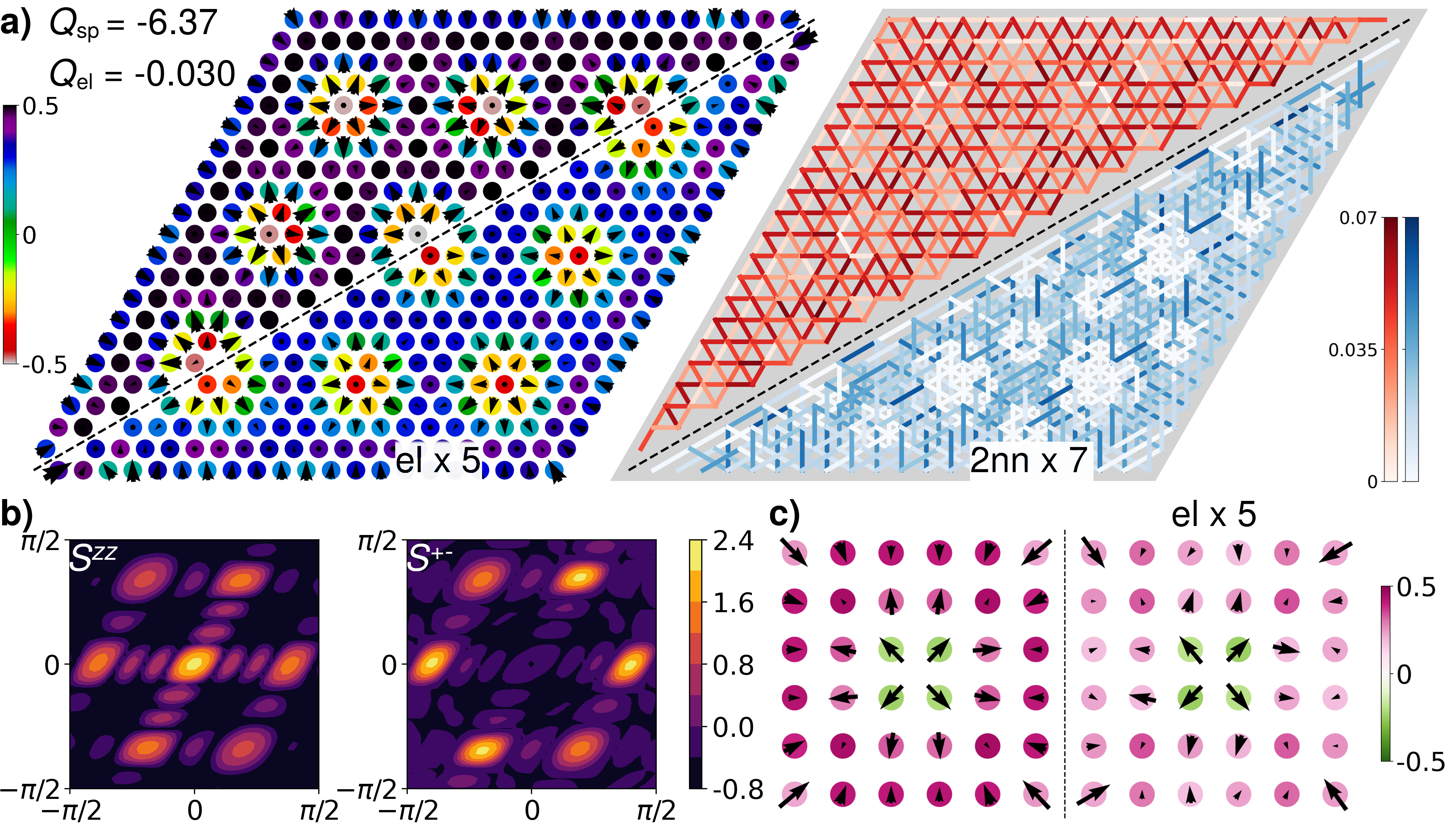
Isolated system.- We consider is a rhombus cluster (which permits to simulate a skyrmion lattice) with open boundary conditions and parameters . The ground state profile of such spin+electron system is shown in Fig. 2a, where the skyrmions exhibit an
approximate periodic alignment, whilst the sites
with state (black circles) can be thought of as domain walls.
Since the l-spins are described quantum mechanically, we can look
at entanglement between spin pairs at sites [63, 64, 37], quantified by the concurrence , and where
is the reduced density matrix. Similarly to what
found in [37], shows a lack of long-range entanglement for the skyrmion (crystal) texture. However, since the distance between sp-el and sp systems is ,
the concurrences with and without i-electrons discernibly differ.
In turn, the i-electrons are affected by the skyrmion texture (for example,
the local density of states for spin-up and spin-down i-electrons
show large (small) imbalance at (far away from) the skyrmions-core sites,
see SM).
Further insight comes from the spin structure factor, defined as , and with denoting either the or the components. In Fig. 2b (for clarity, we show rather than ), both and exhibit sixfold intensity patterns, consistent with neutron scattering results (from e.g. the B20 compound MnSi [3]). Overall, the signal is stronger for than for ; in particular, has a bright spot at , due to the strong degree of spin orientation along . Additionally, the logarithmic display reveals additional but much less intense, lower symmetry features, that we ascribe to size and the open-boundary-conditions effects in the rhombus cluster.
Ground state for an open system. Using NEGF for the i-electrons and Tensor networks for the l-spins, we have also considered the case of a sp-el square cluster attached to leads. The isolated central region ground state at (determined in the mean-field Kondo-exchange) is connected to the leads adiabatically for . The evolution of the sp-el system can then be continued to , which establishes steady spin-polarised currents through the central region in equilibrium. These currents are weak and essentially present only at the boundary sites of (see the SM). The ground state average spin distributions for this setup, with , are shown in Fig. 2d. They result in a value , i.e. a non-strong average influence of the electrons on the spin-texture. Still, a noticeable and interesting feature is that the spins of the i-electrons are tilted compared to the isolated case (not shown). Since for the open case there is a spin-polarized electric current flowing (and a corresponding induced magnetic field), we attribute the spin tilt to an induced effective spin-orbit interaction.
Dynamics. For out-of-equilibrium situations, the natural option would be to consider the open system iii) of Fig. 1c where, after reaching equilibrium at (as discussed above, via a slow-ramping dynamics to connect the leads and dissipate fluctuations), time-dependent currents are injected in the electron subsystem via a bias. For example, for spin-up polarization and with reference to Eq. (2), , where and similar for . The time evolution would then be performed via NEGF for the electrons and via e.g. TEBD for the spins.
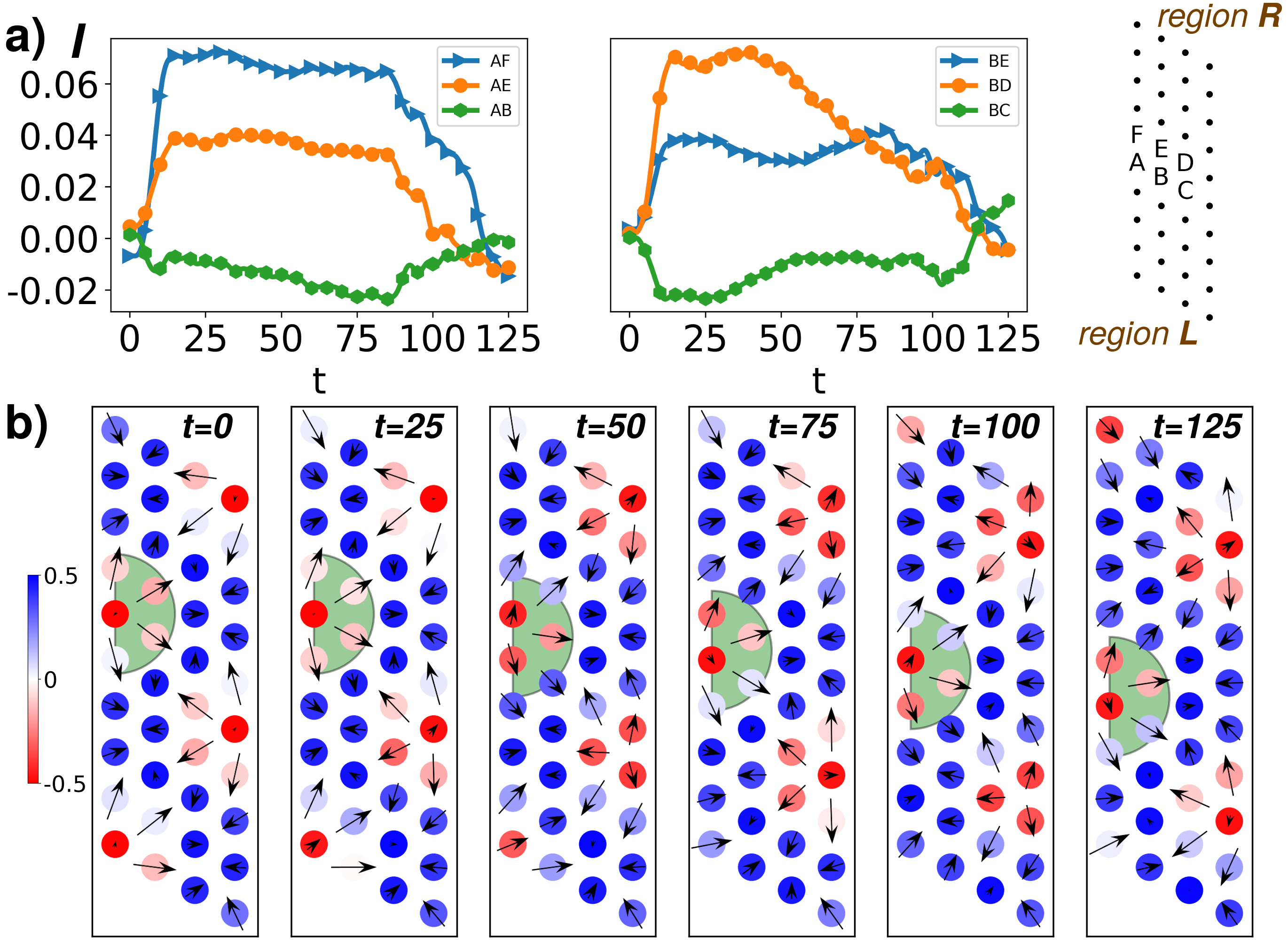
We defer the study of the NEGF+TEBD dynamics of a l-spins+i electrons system connected to semi-infinite leads to a forthcoming paper. Here, as proof of concept of our approach, we use the enlarged isolated setup of Fig. 1b, with a region consisting of a rhombus cluster, and an enlarged electron region of sites, to delay the reflection of the currents by the boundaries, and to have steady, stable currents established within the time of interest. In our simulations, we set . In this case, the (Kondo-exchange mean-field) ground state (obtained without time propagation, and shown at in Fig. 3b) corresponds to a spin texture with multiple meron-like (i.e. half-skyrmion-like) structures. These (henceforth called merons for simplicity) are centered at sites of the cluster boundaries where , with for their second and third neighbours sites . To support this interpretation and address the individual behavior of merons, we use a modified, “local” scalar chirality calculated over all the triangles including sites and (for example, at , for the green shaded meron in Fig. 3b, see SM for details).
Then, starting from , we introduce for a bias with . At each time step of the time evolution, is constructed with input from the time-evolved spin expectation , and the l-spins are evolved via TEBD. Subsequently, an updated and the bias drive the electrons via , and the full spin-electron system is thus evolved for one time step.
The time evolution of selected spin-up bond currents , is shown in Fig. 3a. After the transient regime (), the currents at/near the edges () stay rather stable till ; then, they start to be reflected at the outer boundaries of the regions. By contrast, currents away from the edges () undergo reflection sooner (i.e., ). In Fig. 3a, the currents at different bonds differ for magnitude and/or sign (also for parallel adjacent bonds). This is because of the merons: these are driven in a direction opposite (see the shaded area in the time snapshots) to the average flow of the spin-up electrons (also, small size and nonequilibrium quantum fluctuation make the merons to slightly change their shape in time). The i-electrons, in turn, conform their flow to the presence of the moving merons, which results in the observed behavior of the bond spin-up currents. Furthermore, in the ground state (), the i-electron’s spins texture mirrors the l-spins one, but in a much weaker pattern. The latter extends outside region , while fading as the distance from increases. Yet, with currents (i.e. ), the outer parts of the pattern move towards , affecting the l-spins texture. This is why, for example, at the top-left site in Fig. 3b changes sign during the time evolution.
Conclusions. We have proposed an approach to describe quantum nanoskyrmions in two-dimensional itinerant-electron+localised-spin systems. It combines Matrix Product States methods for the localised-spins, with exact diagonalization or nonequilibrium Green’s function methods for the itinerant electrons, while treating the spin-electron interaction at the mean field level. Our results from different systems and physical setups show that the approach is computationally viable to study in- and out-of-equilibrium quantum skyrmions with itinerant electrons, with a scope different from that of classical-spin+quantum-electron treatments. As future developments, we plan to go beyond a mean-field treatment of the spin-electron interaction via non perturbative local approximations, and to include photon-skyrmion interactions via recent developments in Tensor Networks [65, 66] and nonequilibrium Green’s function formalisms [67].
Acknowledgements.
Z.Z, E.Ö and C.V. gratefully acknowledge financial support from the Swedish Research Council (Vetenskapsrådet, VR, Grant No. 2017-03945 and No. 2022-04486). F.A. gratefully acknowledges financial support from the Swedish Research Council (Vetenskapsrådet, VR, Grant No. 2021-04498_3).References
- Bogdanov and Hubert [1994] A. Bogdanov and A. Hubert, Thermodynamically stable magnetic vortex states in magnetic crystals, J. Magn. Magn. Mater. 138, 255 (1994).
- Rößler et al. [2006] U. K. Rößler, A. N. Bogdanov, and C. Pfleiderer, Spontaneous skyrmion ground states in magnetic metals, Nature 442, 797 (2006).
- Mühlbauer et al. [2009] S. Mühlbauer, B. Binz, F. Jonietz, C. Pfleiderer, A. Rosch, A. Neubauer, R. Georgii, and P. Böni, Skyrmion lattice in a chiral magnet, Science 323, 915 (2009).
- Yu et al. [2010] X. Z. Yu, Y. Onose, N. Kanazawa, J. H. Park, J. H. Han, Y. Matsui, N. Nagaosa, and Y. Tokura, Real-space observation of a two-dimensional skyrmion crystal, Nature 465, 901 (2010).
- Jonietz et al. [2010] F. Jonietz, S. Mühlbauer, C. Pfleiderer, A. Neubauer, W. Münzer, A. Bauer, T. Adams, R. Georgii, P. Böni, R. A. Duine, K. Everschor, M. Garst, and A. Rosch, Spin transfer torques in mnsi at ultralow current densities, Science 330, 1648 (2010).
- Schulz et al. [2012] T. Schulz, R. Ritz, A. Bauer, M. Halder, M. Wagner, C. Franz, C. Pfleiderer, K. Everschor, M. Garst, and A. Rosch, Emergent electrodynamics of skyrmions in a chiral magnet, Nat. Phys. 8, 301 (2012).
- Huang and Chien [2012] S. X. Huang and C. L. Chien, Extended Skyrmion Phase in Epitaxial Thin Films, Phys. Rev. Lett. 108, 267201 (2012).
- Nagaosa and Tokura [2013] N. Nagaosa and Y. Tokura, Topological properties and dynamics of magnetic skyrmions, Nature Nanotechnology 8, 899 (2013).
- Fert et al. [2013] A. Fert, V. Cros, and J. Sampaio, Skyrmions on the track, Nat. Nanotechnol. 8, 152 (2013).
- Fert et al. [2017] A. Fert, N. Reyren, and V. Cros, Skyrmion qubits: Challenges for future quantum computing applications, Nature Reviews Materials 2, 17031 (2017).
- Bhowal and Spaldin [2022] S. Bhowal and N. A. Spaldin, Magnetoelectric classification of skyrmions, Phys. Rev. Lett. 128, 227204 (2022).
- Zhang et al. [2020] X. Zhang, Y. Zhou, K. M. Song, T.-E. Park, J. Xia, M. Ezawa, X. Liu, W. Zhao, G. Zhao, and S. Woo, Skyrmion-electronics: writing, deleting, reading and processing magnetic skyrmions toward spintronic applications, J. Phys.: Condens. Matter 32, 143001 (2020).
- Amoroso et al. [2020] D. Amoroso, P. Barone, and S. Picozzi, Spontaneous skyrmionic lattice from anisotropic symmetric exchange in a ni-halide monolayer, Nature Communications 11, 5784 (2020).
- Yang et al. [2021] S.-H. Yang, R. Naaman, Y. Paltiel, and S. S. P. Parkin, Chiral spintronics, Nature Reviews Physics 3, 328 (2021).
- Psaroudaki and Panagopoulos [2021] C. Psaroudaki and C. Panagopoulos, Skyrmion qubits: A new class of quantum logic elements based on nanoscale magnetization, Phys. Rev. Lett. 127, 067201 (2021).
- Psaroudaki et al. [2023] C. Psaroudaki, E. Peraticos, and C. Panagopoulos, Skyrmion qubits: Challenges for future quantum computing applications, Appl. Phys. Lett. 123, 260501 (2023).
- Szilva et al. [2023] A. Szilva, Y. Kvashnin, E. A. Stepanov, L. Nordström, O. Eriksson, A. I. Lichtenstein, and M. I. Katsnelson, Quantitative theory of magnetic interactions in solids, Rev. Mod. Phys. 95, 035004 (2023).
- Heisenberg [1928] W. Heisenberg, Zur Theorie des Ferromagnetismus, Z. Phys. 49, 619 (1928).
- Dzyaloshinsky [1958] I. Dzyaloshinsky, A thermodynamic theory of “weak” ferromagnetism of antiferromagnetics, J. Phys. Chem. Solids 4, 241 (1958).
- Moriya [1960] T. Moriya, Anisotropic superexchange interaction and weak ferromagnetism, Phys. Rev. 120, 91 (1960).
- Vaz et al. [2008] C. A. F. Vaz, J. A. C. Bland, and G. Lauhoff, Magnetism in ultrathin film structures, Rep. Prog. Phys. 71, 056501 (2008).
- Dieny and Chshiev [2017] B. Dieny and M. Chshiev, Perpendicular magnetic anisotropy at transition metal/oxide interfaces and applications, Rev. Mod. Phys. 89, 025008 (2017).
- Heinze et al. [2011] S. Heinze, K. von Bergmann, , M. Menzel, J. Brede, A. Kubetzka, R. Wiesendanger, G. Bihlmayer, and S. Blügel, Spontaneous atomic-scale magnetic skyrmion lattice in two dimensions, Nat. Phys. 7, 713 (2011).
- Makhfudz et al. [2012] I. Makhfudz, B. Krüger, and O. Tchernyshyov, Inertia and chiral edge modes of a skyrmion magnetic bubble, Phys. Rev. Lett. 109, 217201 (2012).
- Schütte et al. [2014] C. Schütte, J. Iwasaki, A. Rosch, and N. Nagaosa, Inertia, diffusion, and dynamics of a driven skyrmion, Phys. Rev. B 90, 174434 (2014).
- Psaroudaki et al. [2017] C. Psaroudaki, S. Hoffman, J. Klinovaja, and D. Loss, Quantum Dynamics of Skyrmions in Chiral Magnets, Phys. Rev. X 7, 041045 (2017).
- Landau and Lifshitz [1935] L. D. Landau and E. Lifshitz, On the theory of the dispersion of magnetic permeability in ferromagnetic bodies, Phys. Z. Sowjet. 8, 153 (1935).
- Gilbert [2004] T. Gilbert, A phenomenological theory of damping in ferromagnetic materials, IEEE Transactions on Magnetics 40, 3443 (2004).
- Thiele [1973] A. A. Thiele, Steady-State Motion of Magnetic Domains, Phys. Rev. Lett. 30, 230 (1973).
- Ozawa et al. [2017] R. Ozawa, S. Hayami, and Y. Motome, Zero-field skyrmions with a high topological number in itinerant magnets, Phys. Rev. Lett. 118, 147205 (2017).
- Sotnikov et al. [2021] O. M. Sotnikov, V. V. Mazurenko, J. Colbois, F. Mila, M. I. Katsnelson, and E. A. Stepanov, Probing the topology of the quantum analog of a classical skyrmion, Phys. Rev. B 103, L060404 (2021).
- Mazurenko et al. [2023] V. V. Mazurenko, I. A. Iakovlev, O. M. Sotnikov, and M. I. Katsnelson, Estimating patterns of classical and quantum skyrmion states, J. Phys. Soc. Jpn 92, 081004 (2023).
- Haller et al. [2024] A. Haller, S. A. Díaz, W. Belzig, and T. L. Schmidt, Quantum magnetic skyrmion operator (2024), arXiv:2403.10347 [cond-mat.str-el] .
- Peters et al. [2023] R. Peters, J. Neuhaus-Steinmetz, and T. Posske, Quantum skyrmion hall effect in -electron systems, Phys. Rev. Res. 5, 033180 (2023).
- Cirac et al. [2021] J. I. Cirac, D. Pérez-García, N. Schuch, and F. Verstraete, Matrix product states and projected entangled pair states: Concepts, symmetries, theorems, Rev. Mod. Phys. 93, 045003 (2021).
- Lohani et al. [2019] V. Lohani, C. Hickey, J. Masell, and A. Rosch, Quantum skyrmions in frustrated ferromagnets, Phys. Rev. X 9, 041063 (2019).
- Haller et al. [2022] A. Haller, S. Groenendijk, A. Habibi, A. Michels, and T. L. Schmidt, Quantum skyrmion lattices in heisenberg ferromagnets, Phys. Rev. Res. 4, 043113 (2022).
- Joshi et al. [2024] A. Joshi, R. Peters, and T. Posske, Quantum skyrmion dynamics studied by neural network quantum states (2024), arXiv:2403.08184 [cond-mat.dis-nn] .
- Hellman et al. [2017] F. Hellman, A. Hoffmann, Y. Tserkovnyak, G. S. D. Beach, E. E. Fullerton, C. Leighton, A. H. MacDonald, D. C. Ralph, D. A. Arena, H. A. Dürr, P. Fischer, J. Grollier, J. P. Heremans, T. Jungwirth, A. V. Kimel, B. Koopmans, I. N. Krivorotov, S. J. May, A. K. Petford-Long, J. M. Rondinelli, N. Samarth, I. K. Schuller, A. N. Slavin, M. D. Stiles, O. Tchernyshyov, A. Thiaville, and B. L. Zink, Interface-induced phenomena in magnetism, Rev. Mod. Phys. 89, 025006 (2017).
- Viñas Boström and Verdozzi [2019] E. Viñas Boström and C. Verdozzi, Steering magnetic skyrmions with currents: A nonequilibrium green’s functions approach, physica status solidi (b) 256, 1800590 (2019).
- Reyes-Osorio and Nikolic [2023] F. Reyes-Osorio and B. K. Nikolic, Anisotropic skyrmion mass induced by surrounding conduction electrons: A Schwinger-Keldysh field theory approach, arXiv.2302.04220 10.48550/arXiv.2302.04220 (2023).
- Reyes-Osorio and Nikolić [2024] F. Reyes-Osorio and B. K. Nikolić, Gilbert damping in metallic ferromagnets from Schwinger-Keldysh field theory: Intrinsically nonlocal, nonuniform, and made anisotropic by spin-orbit coupling, Phys. Rev. B 109, 024413 (2024).
- Ghosh et al. [2022] S. Ghosh, F. Freimuth, O. Gomonay, S. Blügel, and Y. Mokrousov, Driving spin chirality by electron dynamics in laser-excited antiferromagnets, Communications Physics 5, 69 (2022).
- Ghosh et al. [2023] S. Ghosh, S. Blügel, and Y. Mokrousov, Ultrafast optical generation of antiferromagnetic meron-antimeron pairs with conservation of topological charge, Phys. Rev. Res. 5, L022007 (2023).
- Viñas Boström et al. [2022] E. Viñas Boström, A. Rubio, and C. Verdozzi, Microscopic theory of light-induced ultrafast skyrmion excitation in transition metal films, npj Computational Materials 8, 62 (2022).
- Sahu et al. [2022] P. Sahu, B. R. K. Nanda, and S. Satpathy, Formation of the skyrmionic polaron by rashba and dresselhaus spin-orbit coupling, Phys. Rev. B 106, 224403 (2022).
- Wang and Batista [2023] Z. Wang and C. D. Batista, Skyrmion crystals in the triangular Kondo lattice model, SciPost Phys. 15, 161 (2023).
- Östberg et al. [2023] E. Östberg, E. Viñas Boström, and C. Verdozzi, Microscopic theory of current-induced skyrmion transport and its application in disordered spin textures, Frontiers in Physics 11 (2023).
- Mondal et al. [2021] P. Mondal, A. Suresh, and B. K. Nikolić, When can localized spins interacting with conduction electrons in ferro- or antiferromagnets be described classically via the landau-lifshitz equation: Transition from quantum many-body entangled to quantum-classical nonequilibrium states, Phys. Rev. B 104, 214401 (2021).
- Manchon et al. [2015] A. Manchon, H. C. Koo, J. Nitta, S. M. Frolov, and R. A. Duine, New perspectives for Rashba spin–orbit coupling, Nature Materials 14, 871 (2015).
- Rowland et al. [2016] J. Rowland, S. Banerjee, and M. Randeria, Skyrmions in chiral magnets with rashba and dresselhaus spin-orbit coupling, Phys. Rev. B 93, 020404(R) (2016).
- Fannes et al. [1992] M. Fannes, B. Nachtergaele, and R. F. Werner, Finitely correlated states on quantum spin chains, Commun. Math. Phys. 144, 443 (1992).
- Östlund and Rommer [1995] S. Östlund and S. Rommer, Thermodynamic limit of density matrix renormalization, Phys. Rev. Lett. 75, 3537 (1995).
- Rommer and Östlund [1997] S. Rommer and S. Östlund, Class of ansatz wave functions for one-dimensional spin systems and their relation to the density matrix renormalization group, Phys. Rev. B 55, 2164 (1997).
- Fishman et al. [2022] M. Fishman, S. R. White, and E. M. Stoudenmire, The ITensor Software Library for Tensor Network Calculations, SciPost Phys. Codebases , 4 (2022).
- Paeckel et al. [2019] S. Paeckel, T. Köhler, A. Swoboda, S. R. Manmana, U. Schollwöck, and C. Hubig, Time-evolution methods for matrix-product states, Annals of Physics 411, 167998 (2019).
- Kadanoff and Baym [1962] L. P. Kadanoff and G. Baym, Quantum statistical mechanics : Green’s function methods in equilibrium and nonequilibrium problems (W.A. Benjamin, 1962).
- Keldysh [1964] L. V. Keldysh, Diagram technique for nonequilibrium processes, Sov. Phys. JETP 20, 1018 (1964).
- Balzer and Bonitz [2012] K. Balzer and M. Bonitz, Nonequilibrium Green’s Functions Approach to Inhomogeneous Systems (Springer Berlin, Heidelberg, 2012).
- Stefanucci and van Leeuwen [2013] G. Stefanucci and R. van Leeuwen, Nonequilibrium Many-Body Theory of Quantum Systems: A Modern Introduction (Cambridge University Press, 2013).
- Latini et al. [2014] S. Latini, E. Perfetto, A.-M. Uimonen, R. van Leeuwen, and G. Stefanucci, Charge dynamics in molecular junctions: Nonequilibrium green’s function approach made fast, Phys. Rev. B 89, 075306 (2014).
- Zhang et al. [2023] S. Zhang, X. Li, H. Zhang, P. Cui, X. Xu, and Z. Zhang, Giant Dzyaloshinskii-Moriya interaction, strong XXZ-type biquadratic coupling, and bimeronic excitations in the two-dimensional CrMnI6 magnet, npj Quantum Materials 8, 38 (2023).
- Wootters [1998] W. K. Wootters, Entanglement of formation of an arbitrary state of two qubits, Phys. Rev. Lett. 80, 2245 (1998).
- Horodecki et al. [2009] R. Horodecki, P. Horodecki, M. Horodecki, and K. Horodecki, Quantum entanglement, Rev. Mod. Phys. 81, 865 (2009).
- Huggins et al. [2019] W. Huggins, P. Patil, B. Mitchell, K. B. Whaley, and E. M. Stoudenmire, Towards quantum machine learning with tensor networks, Quantum Sci. and Technol. 4, 024001 (2019).
- Shinaoka et al. [2023] H. Shinaoka, M. Wallerberger, Y. Murakami, K. Nogaki, R. Sakurai, P. Werner, and A. Kauch, Multiscale space-time ansatz for correlation functions of quantum systems based on quantics tensor trains, Phys. Rev. X 13, 021015 (2023).
- Pavlyukh et al. [2022] Y. Pavlyukh, E. Perfetto, D. Karlsson, R. van Leeuwen, and G. Stefanucci, Time-linear scaling nonequilibrium Green’s function methods for real-time simulations of interacting electrons and bosons. I. Formalism, Phys. Rev. B 105, 125134 (2022).