A comparison of correspondence analysis with PMI-based word embedding methods

Abstract

Popular word embedding methods such as GloVe and Word2Vec are related to the factorization of the pointwise mutual information (PMI) matrix. In this paper, we link correspondence analysis (CA) to the factorization of the PMI matrix. CA is a dimensionality reduction method that uses singular value decomposition (SVD), and we show that CA is mathematically close to the weighted factorization of the PMI matrix. In addition, we present variants of CA that turn out to be successful in the factorization of the word-context matrix, i.e. CA applied to a matrix where the entries undergo a square-root transformation (ROOT-CA) and a root-root transformation (ROOTROOT-CA). An empirical comparison among CA- and PMI-based methods shows that overall results of ROOT-CA and ROOTROOT-CA are slightly better than those of the PMI-based methods.

Keywords: Word2Vec; GloVe; Variance stabilization; Overdispersion; Singular value decomposition

1 Introduction

Word embeddings, i.e., dense and low dimensional word representations, are useful in various natural language processing (NLP) tasks (Jurafsky  Martin, 2023; Sasaki ., 2023). Three successful methods to derive such word representations are related to the factorization of the pointwise mutual information (PMI) matrix, an important matrix to be analyzed in NLP (Egleston ., 2021; Bae ., 2021; Alqahtani ., 2023). The PMI matrix is a weighted version of the word-context co-occurrence matrix and measures how often two words, a target word and a context word, co-occur, compared with what we would expect if the two words were independent. The analysis of a positive PMI (PPMI) matrix, where all negative values in a PMI matrix are replaced with zero (Turney  Pantel, 2010; Zhang ., 2022; Alqahtani ., 2023), generally leads to a better performance in semantic tasks (Bullinaria  Levy, 2007), and in most applications the PMI matrix is replaced with the PPMI matrix (Salle ., 2016).

The first method, PPMI-SVD, decomposes the PPMI matrix with a singular value decomposition (SVD) (Levy  Goldberg, 2014; Levy ., 2015; Stratos ., 2015; Zhang ., 2022). The second one is GloVe (Pennington ., 2014). GloVe factorizes the logarithm of the word-context matrix with an adaptive gradient algorithm (AdaGrad) (Duchi ., 2011). According to Shi  Liu (2014); Shazeer . (2016), GloVe is almost equivalent to factorizing a PMI matrix shifted by the logarithm of the sum of the elements of a word-context matrix. The third method is Word2Vec’s skip-gram with negative sampling (SGNS) (Mikolov, Chen ., 2013; Mikolov, Sutskever ., 2013). SGNS uses a neural network model to generate word embeddings. Levy  Goldberg (2014) proved that SGNS implicitly factorizes a PMI matrix shifted by the logarithm of the number of negative samples in SGNS.

In this paper we study what correspondence analysis (CA) (Greenacre, 2017; Beh  Lombardo, 2021) has to offer for the analysis of word-context co-occurrence matrices. CA is an exploratory statistical method that is often used for visualization of a low dimensional approximation of a matrix. It is close to the T-test weighting scheme (Curran  Moens, 2002; Curran, 2004), where standardized residuals are studied, as CA is based on the SVD of the matrix of standardized residuals. In the context of document-term matrices, CA has been compared earlier with latent semantic analysis (LSA), where the document-term matrix is also decomposed with an SVD (Dumais ., 1988; Deerwester ., 1990). Although CA is similar to LSA, there is theoretical and empirical research showing that CA is to be preferred over LSA for text categorization and information retrieval (Qi, Hessen, Deoskar  Van der Heijden, 2023; Qi, Hessen  Van der Heijden, 2023).

CA of a two-way contingency table is equivalent to canonical correlation analysis (CCA) of the data in the form of indicator matrices for the row variable and the column variable of the two-way contingency table (Greenacre, 1984). Stratos . (2015) proposed to combine CCA with a square-root transformation of the cell frequencies of the contingency table. In this paper we refer to this procedure as ROOT-CCA, to distinguish it from ROOT-CA introduced later. Stratos . (2015) found that, on word similarity tasks, (1) the performance of CCA is quite bad, but the performance of ROOT-CCA is a marked improvement, and (2) ROOT-CCA outperforms PPMI-SVD, GloVe, and SGNS. However, CA has not yet been linked to PMI-based methods.

A document-term matrix has some similarity to a word-context matrix, as they both use counts. In this paper, mathematically, we show that CA is close to a weighted factorization of the PMI matrix. We also propose a direct weighted factorization of the PMI matrix (PMI-GSVD). Furthermore, we empirically compare the performance of CA with the performance of PMI-based methods on a word similarity task.

In the context of CA, Nishisato . (2021) point out, generally speaking, a two-way contingency table is prone to overdispersion. Overdispersion may negatively affect the performance of CA (Beh ., 2018; Nishisato ., 2021). To deal with this overdispersion, a fourth-root transformation can be used (Field ., 1982; Greenacre, 2009, 2010). The fourth root transformation has been widely discussed and applied (Downing, 1981; Kostensalo ., 2023; France  Heung, 2023). Therefore, in addition to the word-context matrix, CA is also applied to the fourth-root transformation of the word-context matrix (ROOTROOT-CA). Inspired by ROOT-CCA, CA is also applied to the square-root transformation of the word-context matrix (ROOT-CA). Recently, ROOT-CA has been explored in biology (Hsu  Culhane, 2023). The difference between ROOT-CCA and ROOT-CA is discussed in Section 3.3.

In the following section, research objectives are presented. In Section 3 CA, the three variants of CA, and the T-Test weighting scheme are introduced. The three PMI-based methods are described in Section 4. Theoretical relationships between CA and the PMI-based methods are shown in Section 5. In Section 6 we present two corpora to build word vectors and five word similarity datasets to evaluate word vectors. Section 7 illustrates the setup of the empirical study using these two corpora where CA, PMI-SVD, PPMI-SVD, PMI-GSVD, ROOT-CA, ROOTROOT-CA, ROOT-CCA, SGNS, and GloVe are compared. Section 8 presents the results for these methods on word similarity tasks. Section 9 concludes and discusses this paper.

2 Research objectives

Considering the foregoing, this study focuses on word embeddings in NLP. The objective is to explore the relationship between CA and PMI-based methods and compare the performance in word similarity tasks. In addition, we explore the performance of variants of CA, namely ROOT-CA and ROOTROOT-CA.

3 Correspondence analysis

In this section, first we describe correspondence analysis (CA) using a distance interpretation (Benzécri, 1973; Greenacre  Hastie, 1987), which is a popular way to present CA. Then we present CA making use of an objective function, thus making the later comparison with PMI-based methods straightforward. Third, we present three variants of CA in word embedding. Finally, the T-Test weighting scheme (Curran  Moens, 2002; Curran, 2004) is described, as it turns out to be remarkably similar to CA.

A word-context matrix is a matrix with counts, in which the rows and columns are labeled by terms. In each cell a count represents the number of times the row (target) word and the column (context) word co-occur in a text (Jurafsky  Martin, 2023). Consider a word-context matrix denoted as $\bm{X}$ having $I$ rows ($i=1,2,\cdots,I$) and $J$ columns ($j=1,2,\cdots,J$), where the element for row $i$ and column $j$ is $x_{ij}$. The joint observed proportion is $p_{ij}=x_{ij}/x_{++}$, where ”+” represents the sum over the corresponding elements and $x_{++}=\sum_{i}\sum_{j}x_{ij}$. The marginal proportions of target word $i$ and context word $j$ are $p_{i+}=\sum_{j}p_{ij}$ and $p_{+j}=\sum_{i}p_{ij}$, respectively.

3.1 Introduction to CA

CA is an exploratory method for the analysis of two-way contingency tables. It allows to study how the counts in the contingency table depart from statistical independence. Here we introduce CA in the context of the word-context matrix $\bm{X}$. In CA of the matrix $\bm{X}$, first the elements $x_{ij}$ are converted to joint observed proportions $p_{ij}$, and these are transformed into standardized residuals (Greenacre, 2017)

$$\frac{p_{ij}-p_{i+}p_{+j}}{\sqrt{p_{i+}p_{+j}}}.$$ (1)

Then an SVD is applied to this matrix of standardized residuals, yielding

$$\frac{p_{ij}-p_{i+}p_{+j}}{\sqrt{p_{i+}p_{+j}}}=\sum_{k=1}^{\text{min}\left(I-1,J-1\right)}\sigma_{k}u_{ik}v_{jk},$$ (2)

where $\sigma_{k}$ is the $k$th singular value, with singular values in the decreasing order, and $[u_{1k},u_{2k},\cdots,u_{Ik}]^{T}$ and $[v_{1k},v_{2k},\cdots,v_{Jk}]^{T}$ are the $k$th left and right singular vectors, respectively. When $\bm{X}$ has full rank, the maximum dimensionality is $\text{min}\left(I-1,J-1\right)$, where the ${}^{\prime\prime}-1^{\prime\prime}$ is due to the subtraction of elements $p_{i+}p_{+j}$, that leads to a centering of the elements of $\bm{X}$ as $\sum_{i}(p_{ij}-p_{i+}p_{+j})=0=\sum_{j}(p_{ij}-p_{i+}p_{+j}$). Multiplying the singular vectors consisting of elements $u_{ik}$ and $v_{jk}$ by $p_{i+}^{-\frac{1}{2}}$ and $p_{+j}^{-\frac{1}{2}}$, respectively, leads to

$$\frac{p_{ij}}{p_{i+}p_{+j}}-1=\sum_{k=1}^{\text{min}\left(I-1,J-1\right)}\sigma_{k}\phi_{ik}\gamma_{jk},$$ (3)

where $\phi_{ik}=p_{i+}^{-\frac{1}{2}}u_{ik}$ and $\gamma_{jk}=p_{+j}^{-\frac{1}{2}}v_{jk}$. Scores $\phi_{ik},k=1,2,\cdots,K$ and $\gamma_{jk},k=1,2,\cdots,K$ provide the standard coordinates of row point $i$ and column point $j$ in $K$-dimensional space, respectively, because of $\sum_{i}p_{i+}\phi_{ik}=\sum_{j}p_{+j}\gamma_{jk}=0$ and $\sum_{i}p_{i+}\phi_{ik}^{2}=\sum_{j}p_{+j}\gamma_{jk}^{2}=1$. Scores $\phi_{ik}\sigma_{k},k=1,2,\cdots,K$ and $\gamma_{jk}\sigma_{k},k=1,2,\cdots,K$ provide the principle coordinates of row point $i$ and column point $j$ in $K$-dimensional space, respectively. When $K<\text{min}(I-1,J-1)$, the Euclidean distances between these row (column) points approximate so-called $\chi^{2}$-distances between rows (columns) of $\bm{X}$. The squared $\chi^{2}$-distance between rows $i$ and $i^{\prime}$ of $\bm{X}$ is

$$\delta_{ii^{\prime}}^{2}=\sum_{j}\frac{\left(\frac{p_{ij}}{p_{i+}}-\frac{p_{i^{\prime}j}}{p_{i^{\prime}+}}\right)^{2}}{p_{+j}},$$ (4)

and similarly for the chi-squared distance between columns $j$ and $j^{\prime}$. Equation (4) shows that the $\chi^{2}-$distance $\delta_{ii^{\prime}}$ measures the difference between the $i$th vector of conditional proportions $p_{ij}/p_{i+}$ and the $i^{\prime}$th vector of conditional proportions $p_{i^{\prime}j}/p_{i^{\prime}+}$, where more weight is given to the differences in elements $j$ if $p_{+j}$ is relatively smaller compared to other columns.

Although the use of Euclidean distance is standard in CA, Qi, Hessen  Van der Heijden (2023) show that for information retrieval cosine similarity leads to the best performance among Euclidean distance, dot similarity, and cosine similarity. The superiority of cosine similarity also holds in the context of word embedding studies (Bullinaria  Levy, 2007). Therefore, in this paper we use cosine similarity to calculate the similarity of row points and of column points. It is worth noting that $p_{i+}^{-\frac{1}{2}}$ in $\phi_{ik}=p_{i+}^{-\frac{1}{2}}u_{ik}$ and $p_{+j}^{-\frac{1}{2}}$ in $\gamma_{jk}=p_{+j}^{-\frac{1}{2}}v_{jk}$ have no effects on the cosine similarity. Details are in Supplementary materials A. We coin scores $u_{ik}\sigma_{k},k=1,2,\cdots,K$ and $v_{jk}\sigma_{k},k=1,2,\cdots,K$ an alternative coordinates system for CA directly suited for cosine similarity.

The so-called total inertia is

$$\sum_{i}\sum_{j}\frac{\left(p_{ij}-p_{i+}p_{+j}\right)^{2}}{p_{i+}p_{+j}}=\sum_{k=1}^{\text{min}\left(I-1,J-1\right)}\sigma_{k}^{2}.$$ (5)

This illustrates that CA decomposes the total inertia over $\text{min}\left(I-1,J-1\right)$ dimensions. The total inertia equals the well-known Pearson $\chi^{2}$ statistic divided by $x_{++}$, so that the total inertia does not depend on the sample size $x_{++}$. The relative contribution of cell $(i,j)$ to the total inertia is calculated as $\frac{\left(p_{ij}-p_{i+}p_{+j}\right)^{2}}{p_{i+}p_{+j}}/\sum_{i}\sum_{j}\frac{\left(p_{ij}-p_{i+}p_{+j}\right)^{2}}{p_{i+}p_{+j}}$. The relative contribution of the $i$th row ($j$th column) to the $k$th dimension is calculated as $u_{ik}^{2}$ ($v_{jk}^{2}$).

3.2 The objective function of CA

To simplify the later comparison of CA with the other models, we present the objective function that is minimized in CA. The objective function is (Greenacre, 1984, pp. 345-349):

$$\sum_{i,j}p_{i+}p_{+j}\left(\frac{p_{ij}}{p_{i+}p_{+j}}-1-\bm{e}_{i}^{T}\bm{o}_{j}\right)^{2},$$ (6)

where $\bm{e}_{i}$ and $\bm{o}_{j}$ are parameter vectors for target word $i$ and context word $j$, with respect to which the objective function is minimized. The vectors have length $K\leq\text{min}\left(I-1,J-1\right)$. We call the part of the formula to be approximated, i.e. $\left(p_{ij}/p_{i+}p_{+j}-1\right)$, the fitting function and the weighting part $p_{i+}p_{+j}$ the weighting function. Thus, according to (6), CA can be viewed as a weighted matrix factorization of $\left(p_{ij}/p_{i+}p_{+j}-1\right)$ with weighting function $p_{i+}p_{+j}$.

The solution is found using the SVD as in Equation (2). The $K$-dimensional approximation of $\left(p_{ij}/p_{i+}p_{+j}-1\right)$ is

$$\frac{p_{ij}}{p_{i+}p_{+j}}-1\approx\sum_{k=1}^{K}\sigma_{k}\phi_{ik}\gamma_{jk}=\bm{e}_{i}^{T}\bm{o}_{j}.$$ (7)

The matrix $[\bm{e}_{i}^{T}\bm{o}_{j}]$ minimizes (6) amongst all matrices of rank $K$ in a weighted least-squares sense (Greenacre, 1984). The parameter vectors $\bm{e}_{i}$ and $\bm{o}_{j}$ can be represented, for example, as

$$\bm{e}_{i}=[\phi_{i1}\sigma_{1},\phi_{i2}\sigma_{2},\cdots,\phi_{iK}\sigma_{K}]^{T}$$ (8)

and

$$\bm{o}_{j}=[\gamma_{j1},\gamma_{j2},\cdots,\gamma_{jK}]^{T}$$ (9)

As described above, this representation $\bm{e}_{i}$ of target word $i$ has the advantage that the $\chi^{2}$-distance between target words $i$ and $i^{\prime}$ in the original matrix is approximated by the Euclidean distance between $\bm{e}_{i}$ and $\bm{e}_{i^{\prime}}$.

The parameters $\bm{e}_{i}$ can be adjusted by a singular value weighting exponent $p$, i.e., $\bm{e}_{i}=[\phi_{i1}\sigma_{1}^{p},\phi_{i2}\sigma_{2}^{p},\cdots,\phi_{iK}\sigma_{K}^{p}]^{T}$. Correspondingly, the alternative coordinate for the adjusted row $i$ by a singular value weighting exponent is $[u_{i1}\sigma_{1}^{p},u_{i2}\sigma_{2}^{p},\cdots,u_{iK}\sigma_{K}^{p}]^{T}$.

3.3 Three variants of CA for word embeddings

We present three variants of CA. According to Stratos . (2015), word counts can be naturally modeled as Poisson variables. The square-root transformation of a Poisson variable leads to stabilization of the variance (Bartlett, 1936; Stratos ., 2015). Stratos . (2015) proposed to combine CCA with the square-root transformation of the word-context matrix. Even though CA of a contingency table is equivalent to CCA of the data in the form of an indicator matrix, we call the proposal by Stratos . (2015) ROOT-CCA, to distinguish it from the alternative ROOT-CA, discussed later.

ROOT-CCA

In ROOT-CCA, an SVD is performed on the matrix whose typical element is the square root of $x_{ij}/\sqrt{x_{i+}x_{+j}}=p_{ij}/\sqrt{p_{i+}p_{+j}}$, that is

$$\sqrt{\frac{p_{ij}}{\sqrt{p_{i+}{p_{+j}}}}}=\sum_{k=1}^{\text{min}(I,J)}\sigma_{k}u_{ik}v_{jk}.$$ (10)

The reason that Stratos . (2015) ignore $p_{i+}p_{+j}$ in $p_{ij}-p_{i+}p_{+j}$ (compare Equation (2)) is that they believe that, when the sample size $x_{++}$ is large, the first part $p_{ij}/\sqrt{(p_{i+}p_{+j})}$ in $(p_{ij}-p_{i+}p_{+j})/\sqrt{(p_{i+}p_{+j})}$ dominates the expression.

ROOT-CA

Inspired by Stratos . (2015), we present CA of the square-root transformation of the word-context matrix (ROOT-CA) (Bartlett, 1936; Hsu  Culhane, 2023). ROOT-CA differs from ROOT-CCA in the following way. In the ROOT-CA, first we create a square-root transformation of the word-context matrix with elements $\sqrt{x_{ij}}$, and then we perform CA on this matrix. Let $p_{ij}^{*}=\frac{\sqrt{x_{ij}}}{\sum_{ij}\sqrt{x_{ij}}}=\frac{\sqrt{p_{ij}}}{\sum_{ij}\sqrt{p_{ij}}}$. Then ROOT-CA provides the decomposition

$$\frac{p_{ij}^{*}-p_{i+}^{*}p_{+j}^{*}}{\sqrt{p_{i+}^{*}p_{+j}^{*}}}=\sum_{k=1}^{\text{min}(I-1,J-1)}\sigma_{k}u_{ik}v_{jk}.$$ (11)

ROOTROOT-CA

According to Stratos . (2015), word counts can be naturally modeled as Poisson variables. In the Poisson distribution the mean and variance are identical. The phenomenon of the data having greater variability than expected based on a statistical model is called overdispersion (Agresti, 2007). In the context of CA, Nishisato . (2021) point out, generally speaking, a two-way contingency table is prone to overdispersion. Overdispersion may negatively affect the performance of CA (Beh ., 2018; Nishisato ., 2021).

Greenacre (2009, 2010), referring to Field . (1982), points out that in ecology abundance data is almost always highly over-dispersed and a particular school of ecologists routinely applies a fourth-root transformation before proceeding with the statistical analysis. Therefore we also study the effect of a root-root transformation before performing CA. We call it ROOTROOT-CA. That is, ROOTROOT-CA is a CA on the matrix with typical element $\sqrt{\sqrt{x_{ij}}}$ (Field ., 1982). Suppose $p_{ij}^{**}=\frac{\sqrt{\sqrt{x_{ij}}}}{\sum_{ij}\sqrt{\sqrt{x_{ij}}}}=\frac{\sqrt{\sqrt{p_{ij}}}}{\sum_{ij}\sqrt{\sqrt{p_{ij}}}}$. Then, we have

$$\frac{p_{ij}^{**}-p_{i+}^{**}p_{+j}^{**}}{\sqrt{p_{i+}^{**}p_{+j}^{**}}}=\sum_{k=1}^{\text{min}(I-1,J-1)}\sigma_{k}u_{ik}v_{jk},$$ (12)

Thus ROOT-CA and ROOTROOT-CA are pre-transformations of the elements $x_{ij}$ of the original matrix by $\sqrt{x_{ij}}$ and $\sqrt{\sqrt{x_{ij}}}$, respectively. CA is performed on the transformed matrix.

3.4 T-Test

The T-Test (TTEST) weighting scheme, described by Curran  Moens (2002) and Curran (2004), focuses on the matrix of standardized residuals, see Equation (1). Thus it is remarkably similar to CA, where the matrix of standardized residuals is decomposed. For a comparison between CA and TTEST weighting in word similarity tasks, as we will carry out below, the question is whether the performance is better on the matrix of standardized residuals, or on a low dimensional representation of this matrix provided by CA.

Inspired by Section 3.3, we also explore the performances of the matrix STRATOS-TTEST with typical element $\sqrt{p_{ij}/\sqrt{p_{i+}{p_{+j}}}}$ (compare Equation (10)), the matrix ROOT-TTEST with typical element $\left(p_{ij}^{*}-p_{i+}^{*}p_{+j}^{*}\right)/\sqrt{p_{i+}^{*}p_{+j}^{*}}$ (compare Equation (11)), and the matrix ROOTROOT-TTEST with typical element $\left(p_{ij}^{**}-p_{i+}^{**}p_{+j}^{**}\right)/\sqrt{p_{i+}^{**}p_{+j}^{**}}$ (compare Equation (12)).

4 PMI-based word embedding methods

4.1 PMI-SVD and PPMI-SVD

Pointwise mutual information (PMI) is an important concept in NLP. The PMI between a target word $i$ and a context word $j$ is defined as (Bullinaria  Levy, 2007; Levy  Goldberg, 2014; Levy ., 2015; Jurafsky  Martin, 2023):

$$\text{PMI}(i,j)=\text{log }\frac{p_{ij}}{p_{i+}p_{+j}}$$ (13)

i.e. the log of the contingency ratios (Greenacre, 2009, 2017), also known as Pearson ratios (Goodman, 1996; Beh  Lombardo, 2021), ${p_{ij}}/\left(p_{i+}p_{+j}\right)$. If $p_{ij}=0$, then $\text{PMI}(i,j)=\text{log }0=-\infty$, and it is usual to set $\text{PMI}(i,j)=0$ in this situation.

A common approach is to factorize the PMI matrix using SVD, which we call PMI-SVD. Thus the objective function is

$$\sum_{i,j}\left(\text{log }\frac{p_{ij}}{p_{i+}p_{+j}}-\bm{e}_{i}^{T}\bm{o}_{j}\right)^{2}.$$ (14)

In terms of a weighted matrix factorization, PMI-SVD is the matrix factorization of the PMI matrix with the weighting function $1$. The solution is provided directly via SVD. An SVD applied to the PMI matrix with elements $\text{log}\left(p_{ij}/\left(p_{i+}p_{+j}\right)\right)$ yields

$$\text{log }\frac{p_{ij}}{p_{i+}p_{+j}}=\sum_{k=1}^{\text{min}(I,J)}\sigma_{k}u_{ik}v_{jk},$$ (15)

where $\text{min}(I,J)$ is the rank of the PMI matrix. The $K$-dimensional approximation of $\text{log}\left(p_{ij}/\left(p_{i+}p_{+j}\right)\right)$ is

$$\text{log }\frac{p_{ij}}{p_{i+}p_{+j}}\approx\sum_{k=1}^{K}\sigma_{k}u_{ik}v_{jk}=\bm{e}_{i}^{T}\bm{o}_{j}$$ (16)

where the matrix with elements $\bm{e}_{i}^{T}\bm{o}_{j}$ minimizes (14) amongst all matrices of rank $K$ in a least squares sense, where $K\leq\text{min}(I,J)$. Both CA and PMI-SVD are dimensionality reduction techniques making use of SVD.

The parameters $\bm{e}_{i}$ and $\bm{o}_{j}$ can be represented as

$$\bm{e}_{i}=\left[u_{i1}\sigma_{1},u_{i2}\sigma_{2},\cdots,u_{iK}\sigma_{K}\right]^{T}$$ (17)

and

$$\bm{o}_{j}=\left[v_{j1},v_{j2},\cdots,v_{jK}\right]^{T}.$$ (18)

Thus the Euclidean distance between target words $i$ and $i^{\prime}$ in the original matrix is approximated by the Euclidean distance between $\bm{e}_{i}$ and $\bm{e}_{i^{\prime}}$. In practice, one regularly sees that the parameters $\bm{e}_{i}$ are adjusted by an exponent $p$ used for weighting the singular values, i.e., $\bm{e}_{i}=\left[u_{i1}\sigma_{1}^{p},u_{i2}\sigma_{2}^{p},\cdots,u_{iK}\sigma_{K}^{p}\right]^{T}$, where $p$ is usually set to 0 or 0.5 (Levy  Goldberg, 2014; Levy ., 2015; Stratos ., 2015).

It is worth noting that the elements in the PMI matrix, where word-context pairs that co-occur rarely are negative, but word-context pairs that never co-occur are set to 0 (Levy  Goldberg, 2014), are not monotonic transformations of observed counts divided by counts under independence. For this reason an alternative is proposed, namely the positive PMI matrix, abbreviated as PPMI matrix. In the PPMI matrix all negative values are set to 0:

$$\text{PPMI}(i,j)=\text{max}\left(\text{PMI}(i,j),0\right)$$ (19)

In most applications, one makes use of the PPMI matrix instead of the PMI matrix (Salle ., 2016). We call the factorization of the PPMI matrix using SVD PPMI-SVD (Zhang ., 2022).

4.2 GloVe

The GloVe objective function to be minimized is (Pennington ., 2014):

$$\sum_{i,j}f(x_{ij})\left(\text{log }x_{ij}-b_{i}-s_{j}-\bm{e}_{i}^{T}\bm{o}_{j}\right)^{2}$$ (20)

where

$$f(x_{ij})=\begin{cases}\left(x_{ij}/x_{\text{max}}\right)^{\alpha}&\text{if}\,x_{ij}<x_{\text{max}}\\ 1&\,\text{otherwise}\\ \end{cases}$$

In addition to parameter vectors $\bm{e}_{i}$ and $\bm{o}_{j}$, the scalar parameter terms $b_{i}$ and $s_{j}$ are referred to as $bias$ of target word $i$ and context word $j$, respectively. Pennington . (2014) train the GloVe model using an adaptive gradient algorithm (AdaGrad) (Duchi ., 2011). This algorithm trains only on the non-zero elements of a word-context matrix, as $f(0)=0$, which avoids the appearance of the undefined $\text{log }0$ in Equation (20).

In the original proposal of GloVe (Pennington ., 2014), $b_{i}=\text{log }x_{i+}$ and then, due to the symmetric role of target word and context word, $s_{j}=\text{log }x_{+j}$. Shi  Liu (2014) and Shazeer . (2016) show that the bias terms $b_{i}$ and $s_{j}$ are highly correlated with $\text{log }x_{i+}$ and $\text{log }x_{+j}$, respectively, in GloVe model training. This means that the GloVe model minimizes a weighted least squares loss function with the weighting function $f(x_{ij})$ and approximate fitting function $\text{log}\,x_{ij}-\text{log}\,x_{i+}-\text{log}\,x_{+j}=\text{log}\left(x_{ij}x_{++}/\left(x_{i+}x_{+j}\right)\right)-\text{log}\,x_{++}=\text{log}\left(p_{ij}/\left(p_{i+}p_{+j}\right)\right)-\text{log}\,x_{++}$:

$$\sum_{i,j}f(x_{ij})\left(\text{log }\frac{p_{ij}}{p_{i+}p_{+j}}-\text{log }x_{++}-\bm{e}_{i}^{T}\bm{o}_{j}\right)^{2}$$ (21)

4.3 Skip-gram with negative sampling

SGNS stands for skip-gram with negative sampling of word2vec embeddings (Mikolov, Chen ., 2013; Mikolov, Sutskever ., 2013). The algorithms used in SGNS are stochastic gradient descent and backpropagation (Rumelhart ., 1986; Rong, 2014). SGNS trains word embeddings on every word of the corpus one by one.

Levy  Goldberg (2014) showed that SGNS implicitly factorizes a PMI matrix shifted by $\text{log }n$:

$$\text{log }\frac{p_{ij}}{p_{i+}p_{+j}}-\text{log }n\approx\bm{e}_{i}^{T}\bm{o}_{j}$$ (22)

where $n$ is the number of negative samples. According to Levy  Goldberg (2014) and Shazeer . (2016), the objective function of SGNS is approximately a minimization of the difference between $\bm{e}_{i}^{T}\bm{o}_{j}$ and $\text{log }\left(p_{ij}/\left(p_{i+}p_{+j}\right)-\text{log }n\right)$, tempered by a monotonically increasing weighting function of the observed co-occurrence count $x_{ij}$, that we denote by $g(x_{ij})$:

$$\sum_{i,j}g(x_{ij})\left(\text{log }\frac{p_{ij}}{p_{i+}p_{+j}}-\text{log }n-\bm{e}_{i}^{T}\bm{o}_{j}\right)^{2}$$ (23)

This shows that SGNS differs from GloVe in the use of $n$ instead of $x_{++}$, and $g(x_{ij})$ instead of $f(x_{ij})$.

5 Relationships of CA to PMI-based models

5.1 CA and PMI-SVD / PPMI-SVD

In this section, we discuss PMI-SVD and PPMI-SVD together, as PMI and PPMI are the same except that in PPMI all negative values of PMI are set to 0.

CA is closely related to PMI-SVD. This becomes clear by comparing $\left(p_{ij}/\left(p_{i+}p_{+j}\right)-1\right)$ in (6) with $\text{PMI}(i,j)=\text{log}\left(p_{ij}/\left(p_{i+}p_{+j}\right)\right)$ in (14). The relation lies in a Taylor expansion of $\text{log}\left(p_{ij}/\left(p_{i+}p_{+j}\right)\right)$, namely that, if $x$ is small, $\text{log}(1+x)\approx x$ (Van der Heijden ., 1989). Substituting $x$ with $p_{ij}/(p_{i+}p_{+j})$ – 1 leads to:

$$\text{log }\frac{p_{ij}}{p_{i+}p_{+j}}\approx\frac{p_{ij}}{p_{i+}p_{+j}}-1$$ (24)

This illustrates that if $\left(p_{ij}/p_{i+}p_{+j}-1\right)$ is small, the objective function of CA approximates

$$\sum_{i,j}p_{i+}p_{+j}\left(\text{log }\frac{p_{ij}}{p_{i+}p_{+j}}-\bm{e}_{i}^{T}\bm{o}_{j}\right)^{2}.$$ (25)

From Equation (25) it follows that CA is approximately a weighted matrix factorization of $\text{log }\left(p_{ij}/\left(p_{i+}p_{+j}\right)\right)$ with weighting function $p_{i+}p_{+j}$. The Equation (24) can also be obtained by the Box-Cox transformation of the contingency ratios, for example, Greenacre (2009) and Beh  Lombardo (2024), and we refer to their work for more details.

Comparing Equation (25) with Equation (14), both CA and PMI-SVD can be taken as weighted least squares methods having approximately the same fitting functions, namely $\left(p_{ij}/p_{i+}p_{+j}-1\right)$ for CA and $\text{log}\left(p_{ij}/\left(p_{i+}p_{+j}\right)\right)$ for PMI-SVD. Both make use of an SVD.

However, they use different weighting functions, namely $p_{i+}p_{+j}$ in CA and $1$ in PMI-SVD. It has been argued that equally weighting errors in the objective function, as is the case in PMI-SVD, is not a good approach (Salle ., 2016; Salle  Villavicencio, 2023). For example, Salle  Villavicencio (2023) presented the reliability principle, that the objective function should have a weight on the reconstruction error that is a monotonically increasing function of the marginal frequencies of word and of context. On the other hand, CA, unlike PMI-SVD, weights errors in the objective function with a weighting function equal to the product of the marginal proportions of word and context (Greenacre, 1984, 2017; Beh  Lombardo, 2021).

5.1.1 PMI-GSVD

The weighting function of PMI-SVD is 1 while in the approximate version of CA it is $p_{i+}p_{+j}$. Therefore, we also investigate the performance of a weighted factorization of the PMI matrix, where $p_{i+}p_{+j}$ is the weighting function:

$$\sum_{i,j}p_{i+}p_{+j}\left(\text{log }\frac{p_{ij}}{p_{i+}p_{+j}}-\bm{e}_{i}^{T}\bm{o}_{j}\right)^{2}.$$ (26)

Similar with CA, we use generalized SVD (GSVD) to find the optimum of the objective function (PMI-GSVD). That is, an SVD is applied as follows:

$$\sqrt{p_{i+}p_{+j}}\,\text{log }\frac{p_{ij}}{p_{i+}p_{+j}}=\sum_{k=1}^{\text{min}(I,J)}\sigma_{k}u_{ik}v_{jk},$$ (27)

We call the matrix with typical element $\sqrt{p_{i+}p_{+j}}\,\text{log }\frac{p_{ij}}{p_{i+}p_{+j}}$ the WPMI matrix, also known as the modified log-likelihood ratio residual (Beh  Lombardo, 2024).

5.2 CA and GloVe

Both CA and GloVe are weighted least squares methods. The weighting function in GloVe is $f(x_{ij})$, which is defined uniquely for each element of the word-context matrix, while the weighting function $p_{i+}p_{+j}$ in CA is defined by the row and column margins.

In the approximate fitting function of GloVe, $\text{log}\left(p_{ij}/\left(p_{i+}p_{+j}\right)\right)-\text{log }x_{++}$, the term $\text{log }x_{++}$ can be considered as a shift of $\text{log}\left(p_{ij}/\left(p_{i+}p_{+j}\right)\right)$. And as we showed in Section 5.1, the fitting function of CA is approximately $\text{log}\left(p_{ij}/\left(p_{i+}p_{+j}\right)\right)$ when $p_{ij}$ is close to $p_{i+}p_{+j}$. Thus, from a comparison of the objective functions of CA and GloVe, it is natural to expect that these two methods will yield similar results if $\left(p_{ij}/p_{i+}p_{+j}-1\right)$ is small.

In comparing the algorithms of these two methods, we find that CA uses SVD while GloVe uses AdaGrad. These two algorithms have their own advantages and disadvantages. On the one hand, the AdaGrad algorithm trains GloVe only on the nonzero elements of word-context matrix, one by one, while in CA the SVD decomposes the entire word-context matrix in full in one step. On the other hand, the SVD always finds the global minimum while the AdaGrad algorithm cannot guarantee the global minimum.

5.3 CA and SGNS

By comparing Equations (23) and (25), both the approximation of CA and of SGNS are found by weighted least squares methods. The weighting function in SGNS is $g(x_{ij})$, which is defined for each element of word-context matrix where frequent word-context pairs pay more for deviations than infrequent ones (Levy  Goldberg, 2014), while the weighting function in CA is defined by the row and column margins, i.e. $p_{i+}p_{+j}$.

In the fitting function of the approximation of SGNS, $\text{log}\left(p_{ij}/\left(p_{i+}p_{+j}\right)\right)-\text{log }n$, the term $\text{log }n$ can be considered as a shift of $\text{log}\left(p_{ij}/\left(p_{i+}p_{+j}\right)\right)$. As shown in Section 5.1, the approximate fitting function in CA is $\text{log}\left(p_{ij}/\left(p_{i+}p_{+j}\right)\right)$. Thus, considering the objective function view, both the approximation of CA and of SGNS make use of the PMI matrix.

Although the approximate objective function of SGNS is similar to that of CA, the training processing for SGNS is different from that of CA. SGNS trains word embeddings on the words of a corpus, one by one, to maximize the probabilities of target words and context words co-occurrence, and to minimize the probabilities between target words and randomly sampled words, by updating the vectors of target words and context words. In contrast, CA first counts all co-occurrences in the corpus and then performs SVD on the matrix of standardized residuals to obtain the vectors of target words and context words at once.

6 Two corpora and five word similarity datasets

All methods are trained on two corpora: Text8 (Text8 dataset, 2006) and British National Corpus (BNC) (BNC Consortium, 2007), respectively. Text8 is a widely used corpus in NLP (Xin ., 2018; Roesler ., 2019; Podkorytov ., 2020; Guo  Yao, 2021). It includes more than 17 million words from Wikipedia (Peng  Feldman, 2017) and only consists of lowercase English characters and spaces. Words that appeared less than 100 times in the corpus are ignored, resulting in a vocabulary of 11,815 terms.

BNC is from a representative variety of sources and is widely used (Raphael, 2023; Samuel ., 2023). Data cited herein have been extracted from the British National Corpus, distributed by the University of Oxford on behalf of the BNC Consortium. We remove English punctuation and numbers and set words in lowercase form. Words that appeared less than 500 times in the corpus are ignored, resulting in a vocabulary of 11,332 terms.

Following previous studies (Levy ., 2015; Pakzad  Analoui, 2021), we evaluate each word embeddings method on word similarity tasks using the Spearman’s correlation coefficient $\rho$. We use five popular word similarity datasets: WordSim353 (Finkelstein ., 2002), MEN (Bruni ., 2012), Mechanical Turk (Radinsky ., 2011), Rare (Luong ., 2013), and SimLex-999 (Hill ., 2015). All these datasets consist of word pairs together with human-assigned similarity scores. For example, in WordSim353, where scores range from 0 (least similar) to 10 (most similar), one word pair is (tiger, cat) with human assigned similarity score 7.35. Out-of-vocabulary words are removed from all test sets. I.e., if either tiger or cat doesn’t occur in the vocabularies of the 11,815 terms created by Text8 corpus, we delete (tiger, cat). Thus for evaluating the different word embedding methods in Text8 277 word pairs with scores are kept in WordSim353 instead of the original 353 word pairs. Table 1 provides the number of word pairs used by the datasets in Text8 and BNC.

Table 1: Datasets for word similarity evaluation.

Dataset	Word pairs	Word pairs in Text8	Word pairs in BNC
WordSim353	353	277	276
MEN	3000	1544	1925
Turk	287	221	197
Rare	2034	205	204
SimLex-999	999	726	847

After calculating the solutions for CA, PMI-SVD, PPMI-SVD, PMI-GSVD, ROOT-CA, ROOTROOT-CA, ROOT-CCA, GloVe, and SGNS, we obtain the word embeddings. We calculate the cosine similarity for each word pair in each word similarity dataset. For example, for WordSim353 using Text8, we obtain 277 cosine similarities. The Spearman’s correlation coefficient $\rho$ (Hollander ., 2013) between these similarities and the human similarity scores is calculated to evaluate these word embedding methods. Larger values are better.

7 Study setup

7.1 SVD-based methods

CA, PMI-SVD, PPMI-SVD, PMI-GSVD, ROOT-CA, ROOTROOT-CA, and ROOT-CCA are SVD-based dimensionality reduction methods. First, we create a word-context matrix of size 11,815$\times$11,815 and 11,332$\times$11,332 based on Text8 and BNC, respectively. We use a window of size 2, i.e., two words to each side of the target word. A context word one token and two tokens away will be counted as $1/1$ and $1/2$ of an occurrence, respectively. Then we perform SVD on the related matrices. We use the svd function from scipy.linalg in Python to calculate the SVD of a matrix, and obtain singular values $\sigma_{k}$, left singular vectors $u_{ik}$, and right singular vectors $v_{jk}$. We obtain the word embeddings as $\bm{e}_{i}=\left[u_{i1}\sigma_{1}^{p},u_{i2}\sigma_{2}^{p},\cdots,u_{ik}\sigma_{k}^{p}\right]^{T}$.

The choices of the exponent weighting $p$ and number of dimensions $k$ are important for SVD-based methods. In the context of PPMI-SVD and ROOT-CCA $p$ is regularly set to $p=0$ or $p=0.5$ (Levy  Goldberg, 2014; Levy ., 2015; Stratos ., 2015). For $p=0$, we have the standard coordinates with $\bm{U}^{T}\bm{U}=\bm{V}^{T}\bm{V}=\bm{I}$. For $p=0.5$, we have $\bm{A}_{k}=\bm{U}_{k}\bm{\Sigma}_{k}\bm{V}_{k}^{T}=(\bm{U}_{k}\bm{\Sigma}_{k}^{1/2})(\bm{V}_{k}\bm{\Sigma}_{k}^{1/2})^{T}$. That is, the target words $\bm{U}_{k}\bm{\Sigma}_{k}^{1/2}$ and context words $\bm{V}_{k}\bm{\Sigma}_{k}^{1/2}$ reconstruct the decomposed matrix $\bm{A}_{k}$. The two created word-context matrices based on Text8 and BNC are symmetric, so the matrices to be decomposed are also symmetric. For the SVD of a symmetric matrix, using the target words $\bm{U}_{k}\bm{\Sigma}_{k}^{1/2}$ for word embeddings is equivalent to using the context words $\bm{V}_{k}\bm{\Sigma}_{k}^{1/2}$ for word embeddings. We vary the number of dimensions $k$ from 2, 50, 100, 200, $\cdots$, 1,000, 2,000, $\cdots$, 10,000.

7.2 GloVe and SGNS

We use the public implementation by Pennington . (2014) to perform GloVe and choose the default hyperparameters. Pennington . (2014) proposed to use the context vectors $\bm{o}_{j}$ in addition to target word vectors $\bm{e}_{i}$. Here, we only use target word vectors $\bm{e}_{i}$, set window size to 2 and set vocab minimum count to 100 for Text8 and 500 for BNC, in the same way as for the SVD-based methods to keep the settings consistent. We vary the dimension $k$ of word embeddings from 200 to 600 with intervals of 100.

We use the public implementation by Mikolov, Sutskever . (2013) to perform SGNS, and use the vocabulary created by GloVe as the input of SGNS. We choose the default values except for the dimensions $k$ of word embeddings and window size, which are chosen in the same way as in GloVe, to keep the settings consistent.

8 Results

We make a distinction between conditions where no dimensionality reduction takes place, and conditions where dimensionality reduction is used. For no dimensionality reduction we compare TTEST, PMI, PPMI, WPMI, ROOT-TTEST, ROOTROOT-TTEST, STRATOS-TTEST. For dimensionality reduction we first compare CA with the more standard methods PMI-SVD, PPMI-SVD, PMI-GSVD, GloVe, SGNS, and then compare variants of CA.

8.1 TTEST, PMI, PPMI, WPMI, ROOT-TTEST, ROOTROOT-TTEST, and STRATOS-TTEST

First, we compare methods where no dimensionality reduction takes place. We show the Spearman’s correlation coefficient $\rho$ for the TTEST, PMI, PPMI, WPMI, ROOT-TTEST, ROOTROOT-TTEST, and STRATOS-TTEST matrices in Table 2. The results for the five word similarity datasets and the two corpora show that (1) either ROOT-TTEST or ROOTROOT-TTEST is best, and (2) ROOT-TTEST is consistently better than PPMI, PMI, STRATOS-TTEST, and WPMI. In the Total column of the block at the bottom of the table we provide the sum of $\rho$-values for all five datasets and two corpora. Overall, ROOT-TTEST and ROOTROOT-TTEST perform best, closely followed by PPMI and TTEST. PMI follows at some distance, and last, we find STRATOS-TTEST and WPMI.

Table 2: Correlation coefficient $\rho$ for fitting matrix.

		Text8	BNC	Total
WordSim353	TTEST	0.588	0.427	1.015
	PMI	0.587	0.292	0.879
	PPMI	0.609	0.505	1.115
	WPMI	0.233	0.221	0.454
	ROOT-TTEST	0.658	0.539	1.197
	ROOTROOT-TTEST	0.646	0.495	1.141
	STRATOS-TTEST	0.438	0.314	0.752
MEN	TTEST	0.248	0.260	0.509
	PMI	0.269	0.224	0.494
	PPMI	0.253	0.284	0.537
	WPMI	0.132	0.171	0.303
	ROOT-TTEST	0.305	0.293	0.598
	ROOTROOT-TTEST	0.317	0.263	0.580
	STRATOS-TTEST	0.156	0.130	0.286
Turk	TTEST	0.619	0.649	1.268
	PMI	0.629	0.514	1.143
	PPMI	0.651	0.625	1.276
	WPMI	0.343	0.417	0.760
	ROOT-TTEST	0.666	0.659	1.325
	ROOTROOT-TTEST	0.667	0.616	1.283
	STRATOS-TTEST	0.561	0.525	1.086
Rare	TTEST	0.392	0.428	0.820
	PMI	0.335	0.289	0.624
	PPMI	0.328	0.363	0.691
	WPMI	0.252	0.255	0.506
	ROOT-TTEST	0.389	0.477	0.866
	ROOTROOT-TTEST	0.418	0.454	0.872
	STRATOS-TTEST	0.243	0.196	0.439
SimLex-999	TTEST	0.220	0.230	0.450
	PMI	0.257	0.168	0.425
	PPMI	0.251	0.277	0.528
	WPMI	0.139	0.118	0.257
	ROOT-TTEST	0.276	0.280	0.556
	ROOTROOT-TTEST	0.271	0.239	0.509
	STRATOS-TTEST	0.181	0.125	0.306
Total	TTEST	2.067	1.994	4.061
	PMI	2.078	1.487	3.565
	PPMI	2.092	2.054	4.146
	WPMI	1.098	1.182	2.280
	ROOT-TTEST	2.293	2.249	4.542
	ROOTROOT-TTEST	2.319	2.067	4.386
	STRATOS-TTEST	1.579	1.289	2.869

8.2 CA, PMI-SVD, PPMI-SVD, PMI-GSVD, GloVe, and SGNS

Next, we compare CA (RAW-CA in Table 3) with the PMI-based methods PMI-SVD, PPMI-SVD, PMI-GSVD, GloVe, and SGNS. Table 3 has a left part, where $p=0$, and a right part, where $p=0.5$. As $p$ does not exist in GloVe and SGNS, these methods have identical values for $p=0$ and $p=0.5$. Plots for $\rho$ as a function of $k$ for SVD-based methods are in Supplementary materials B.

Comparing the last block of Table 3 with the last block of Table 2 reveals that, overall, dimensionality reduction is beneficial for the size of $\rho$, as CA, PMI-SVD, PPMI-SVD, PMI-GSVD, ROOT-CA, ROOTROOT-CA, and ROOT-CCA do better than their respective counterparts TTEST, PMI, PPMI, WPMI, ROOT-TTEST, ROOTROOT-TTEST, and STRATOS-TTEST. For TTEST the improvement due to using SVD is less than for PMI, PPMI, WPMI, ROOT-TTEST, STRATOS-TTEST; for WPMI and STRATOS-TTEST the improvement due to using SVD is more than for TTEST, PPMI, ROOT-TTEST, and ROOTROOT-TTEST, which is a result consistent for each corpus and each word similarity dataset.

For an overall comparison of the dimensionality reduction methods, we study the block at the bottom of Table 3, which provides the sum of the $\rho$-values over the five word similarity datasets. For both $p=0$ and $p=0.5$, among RAW-CA, PMI-SVD, PPMI-SVD, PMI-GSVD, GloVe, and SGNS, overall PMI-SVD and PPMI-SVD perform best, closely followed by SGNS. RAW-CA and PMI-GSVD follow at some distance, and last, we find GloVe. The popular method GloVe does not perform well. Possibly the conditions of the study are not optimal for GloVe, as the Text8 and BNC corpora are, with 11,815 and 11,332 terms respectively, possibly too small to obtain reliable results (Jiang ., 2018).

Table 3: SVD: correlation coefficient $\rho$ with $p=0,0.5$.

		$p=0$					$p=0.5$
		Text8		BNC			Text8		BNC
		$k$	$\rho$	$k$	$\rho$	total	$k$	$\rho$	$k$	$\rho$	total
WordSim353	RAW-CA	600	0.578	400	0.465	1.043	9000	0.609	10000	0.498	1.107
	PMI-SVD	400	0.675	600	0.628	1.303	400	0.683	500	0.579	1.262
	PPMI-SVD	400	0.681	700	0.628	1.309	200	0.694	2000	0.623	1.317
	GloVe	200	0.422	600	0.522	0.943	200	0.422	600	0.522	0.943
	SGNS	300	0.668	600	0.551	1.219	300	0.668	600	0.551	1.219
	PMI-GSVD	700	0.512	600	0.468	0.980	6000	0.548	3000	0.449	0.997
	ROOT-CA	300	0.668	400	0.623	1.291	500	0.688	900	0.657	1.345
	ROOTROOT-CA	200	0.692	200	0.635	1.327	300	0.697	400	0.630	1.327
	ROOT-CCA	100	0.682	700	0.627	1.310	300	0.684	600	0.620	1.304
MEN	RAW-CA	300	0.223	600	0.293	0.516	7000	0.256	9000	0.299	0.556
	PMI-SVD	800	0.328	700	0.393	0.721	600	0.317	2000	0.357	0.674
	PPMI-SVD	800	0.336	500	0.394	0.730	800	0.324	1000	0.358	0.681
	GloVe	300	0.175	600	0.310	0.485	300	0.175	600	0.310	0.485
	SGNS	400	0.295	400	0.333	0.627	400	0.295	400	0.333	0.627
	PMI-GSVD	800	0.267	600	0.318	0.585	5000	0.256	3000	0.308	0.564
	ROOT-CA	800	0.325	500	0.400	0.725	9000	0.324	800	0.374	0.698
	ROOTROOT-CA	600	0.340	400	0.396	0.735	1000	0.332	4000	0.359	0.690
	ROOT-CCA	600	0.315	400	0.392	0.706	900	0.298	800	0.355	0.653
Turk	RAW-CA	400	0.549	100	0.562	1.111	400	0.592	10000	0.588	1.181
	PMI-SVD	100	0.656	50	0.652	1.308	300	0.677	500	0.661	1.338
	PPMI-SVD	50	0.668	50	0.671	1.339	50	0.677	50	0.683	1.361
	GloVe	600	0.502	200	0.540	1.042	600	0.502	200	0.540	1.042
	SGNS	200	0.651	300	0.650	1.302	200	0.651	300	0.650	1.302
	PMI-GSVD	900	0.495	200	0.506	1.000	5000	0.563	10000	0.584	1.147
	ROOT-CA	50	0.649	50	0.695	1.344	100	0.661	50	0.684	1.345
	ROOTROOT-CA	50	0.669	50	0.666	1.334	50	0.664	300	0.673	1.337
	ROOT-CCA	50	0.633	50	0.672	1.305	100	0.665	100	0.678	1.343
Rare	RAW-CA	600	0.396	500	0.450	0.846	900	0.411	3000	0.465	0.875
	PMI-SVD	100	0.476	700	0.480	0.957	300	0.471	5000	0.464	0.936
	PPMI-SVD	100	0.483	400	0.470	0.952	100	0.475	6000	0.469	0.944
	GloVe	400	0.181	600	0.379	0.560	400	0.181	600	0.379	0.560
	SGNS	600	0.456	200	0.532	0.988	600	0.456	200	0.532	0.988
	PMI-GSVD	400	0.451	500	0.418	0.869	900	0.431	600	0.429	0.860
	ROOT-CA	400	0.468	400	0.501	0.970	600	0.479	7000	0.526	1.006
	ROOTROOT-CA	100	0.503	500	0.476	0.978	100	0.475	4000	0.478	0.953
	ROOT-CCA	200	0.469	200	0.505	0.974	600	0.469	900	0.511	0.979
SimLex-999	RAW-CA	4000	0.219	2000	0.322	0.541	8000	0.243	7000	0.327	0.571
	PMI-SVD	700	0.310	900	0.409	0.719	3000	0.315	900	0.372	0.687
	PPMI-SVD	700	0.309	500	0.393	0.702	3000	0.308	500	0.368	0.676
	GloVe	500	0.148	500	0.255	0.403	500	0.148	500	0.255	0.403
	SGNS	600	0.306	400	0.376	0.682	600	0.306	400	0.376	0.682
	PMI-GSVD	900	0.272	4000	0.365	0.637	5000	0.271	3000	0.312	0.583
	ROOT-CA	2000	0.295	900	0.415	0.710	5000	0.309	2000	0.395	0.704
	ROOTROOT-CA	700	0.321	900	0.410	0.731	700	0.317	900	0.376	0.693
	ROOT-CCA	1000	0.294	1000	0.421	0.715	7000	0.303	2000	0.391	0.693
total	RAW-CA		1.965		2.092	4.057		2.111		2.178	4.290
	PMI-SVD		2.445		2.562	5.007		2.465		2.433	4.897
	PPMI-SVD		2.476		2.556	5.033		2.478		2.501	4.979
	GloVe		1.427		2.006	3.433		1.427		2.006	3.433
	SGNS		2.376		2.442	4.819		2.376		2.442	4.819
	PMI-GSVD		1.997		2.075	4.072		2.069		2.082	4.151
	ROOT-CA		2.405		2.635	5.039		2.462		2.637	5.098
	ROOTROOT-CA		2.525		2.582	5.107		2.484		2.515	4.999
	ROOT-CCA		2.393		2.617	5.011		2.417		2.555	4.972

As the focus in this paper is on the performance of CA, we give some extra attention to RAW-CA and the similar PMI-GSVD. Even though CA and PMI-GSVD have the same weighting function $p_{i+}p_{+j}$, and should be close when $p_{ij}/\left(p_{i+}p_{+j}\right)-1$ is small (compare the discussion around Equations (24, 25)) their performances are rather different. This may be because there are extremely large values (larger than 35,000) in the fitting function $\left(p_{ij}/\left(p_{i+}p_{+j}\right)-1\right)$ of CA, which makes the fitting function of CA not close to the fitting function log $\left(p_{ij}/\left(p_{i+}p_{+j}\right)\right)$ of PMI-GSVD.

When we compare PMI-GSVD with PMI-SVD, we are surprised to find that weighting rows and columns appears to decrease the values of $\rho$. This is in contrast with the reliability principle of Salle  Villavicencio (2023) discussed above.

We now discuss why PMI-SVD and PPMI-SVD do better than PMI-GSVD. It turns out that the number and sizes of extreme values in the matrix WPMI decomposed by PMI-GSVD are much larger than in PMI and PPMI, and this results in PMI-GSVD dimensions being dominated by single words. We only include non-zero elements in the PMI matrix as the PMI matrix is sparse: 94.2% of the entries are zero for Text8; for a fair comparison, the corresponding 94.2% of entries in the PPMI and WPMI matrices are also ignored. Following box plot methodology (Tukey, 1977; Schwertman ., 2004; Dodge, 2008), extreme values are determined as follows: let $q_{1}$ and $q_{3}$ be the first and third sample quartiles, and let $f_{1}=q_{1}-1.5(q_{3}-q_{1})$, $f_{3}=q_{3}+1.5(q_{3}-q_{1})$. Then extreme values are defined as values less than $f_{1}$ (LT$f_{1}$) or greater than $f_{3}$ (GT$f_{3}$). The first three rows in Table 4 show the number of extreme elements in the PMI, PPMI, WPMI matrices. The number of extreme values of the WPMI matrix (1,384,231) is much larger than that of PMI and PPMI (32,319 and 27,984). Furthermore, in WPMI the extremeness of values is much larger than in PMI and PPMI. Let the averaged contribution of each cell, expressed as a proportion, be $1/\left(11,815\times 11,815\right)$. However, in WPMI, the most extreme entry, found for (the, the), contributes around 0.01126 to the total inertia. In PMI (PPMI) the most extreme entry is (guant, namo) or (namo, guant) and contributes around $3.1\times 10^{-6}$ ($3.2\times 10^{-6}$) to the total inertia. Figure 1 shows the contribution of the rows for the corresponding to top 10 extreme values, to the first 100 dimensions of PMI-SVD, PPMI-SVD, PMI-GSVD. The rows, corresponding to the top extreme values in the WPMI matrix, take up a much bigger contribution to the first dimensions of PMI-GSVD. For example, in PMI-GSVD, the “the” row contributes more than 0.3 to the third dimension, while in PMI-SVD and PPMI-SVD, the contributions are much more even. Thus the PMI-GSVD solution is hampered by extreme cells in the WPMI matrix that is decomposed. Similar results can be found for BNC in Supplementary materials C.

Table 4: Text8: the number of extreme values

	LT$f_{1}$	GT$f_{3}$	total
PMI	4,335	27,984	32,319
PPMI	0	27,984	27,984
WPMI	1,038,236	345,995	1,384,231
TTEST	50,560	627,046	677,606
ROOT-TTEST	5,985	448,860	454,845
ROOTROOT-TTEST	4,942	396,437	401,379
STRATOS-TTEST	0	400,703	400,703

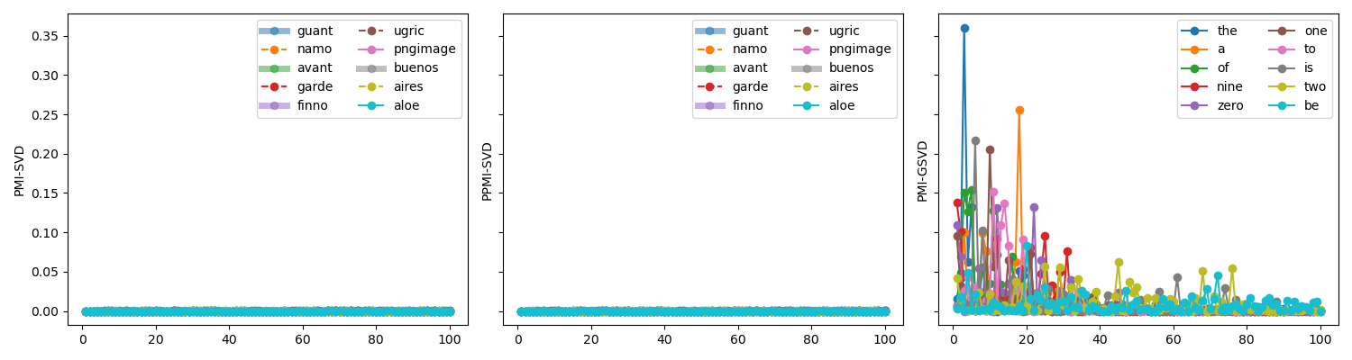
Figure 1: Text8: the contribution of the rows, corresponding to the top 10 extreme values, to the first 100 dimensions of PMI-SVD, PPMI-SVD, PMI-GSVD.

8.3 The results for three variants of CA

Now we compare the three variants of CA (ROOT-CA, ROOTROOT-CA, ROOT-CCA) with CA-RAW and the winner of the PMI-based methods, PPMI-SVD.

First, in Table 3, the three variants of CA perform much better than RAW-CA in each word similarity dataset and each corpus, both for $p=0$ and $p=0.5$. In the block at the bottom of Table 3, overall, the performance of the three variants is similar, where ROOT-CA outperforms ROOT-CCA slightly.

The lower part of Table 4 shows the number of extreme values of TTEST, ROOT-TTEST, ROOTROOT-TTEST and STRATOS-TTEST matrices for Text8. Similar with PMI, PPMI, WPMI, 94.2% of entries are ignored. The number of extreme values of the TTEST matrix (677,606) is larger than that of ROOT-TTEST, ROOTROOT-TTEST and STRATOS-TTEST (454,845, 401,379, and 400,703). Furthermore, in TTEST the extremeness of the extreme values is larger than those in ROOT-TTEST, ROOTROOT-TTEST, and STRATOS-TTEST. For example, in TTEST the most extreme entry (agave, agave) contributes around 0.02117 to the total inertia, while in ROOT-TTEST, ROOTROOT-TTEST, and STRATOS-TTEST, the most extreme entries (agave, agave), (pngimage, pngimage), and (agave, agave) contribute around 0.00325, 0.00119, and 0.00017, respectively. Figure 2 shows the contribution of the rows for the top 10 extreme values, to the first 100 dimensions of RAW-CA, ROOT-CA, and ROOTROOT-CA (The corresponding plot about ROOT-CCA is in Supplementary materials D). In RAW-CA, the rows, corresponding to top extreme values of TTEST, take up a big contribution to the first dimensions of RAW-CA. For example, in RAW-CA, the “agave” row contributes around 0.983 to the first dimension, while in ROOT-CA and ROOTROOT-CA, the contributions are much smaller which also holds for ROOT-CCA. Similar results can be found for BNC in Supplementary materials E. Thus, we infer that the extreme values in TTEST are the important reason that RAW-CA performs badly.

Figure 2: Text8: the contribution of the rows, corresponding to top 10 extreme values, to first 100 dimensions of RAW-CA, ROOT-CA, ROOTROOT-CA.

Second, in the rows of the block at the bottom of Table 3, the overall performances of ROOT-CA, ROOTROOT-CA, ROOT-CCA are comparable to or sometimes slightly better than PPMI-SVD. Specifically, ROOTROOT-CA and ROOT-CA achieve the highest $\rho$ for Text8 and BNC corpora, respectively. Based on these results, no matter what we know about the corpus, ROOTROOT-CA and ROOT-CA appear to have potential to improve the performance in NLP tasks.

9 Conclusion and discussion

PMI is an important concept in natural language processing. In this paper, we theoretically compare CA with three PMI-based methods with respect to their objective functions. CA is a weighted factorization of a matrix where the fitting function is $\left(p_{ij}/\left(p_{i+}p_{+j}\right)-1\right)$ and the weighting function is the product of row margins and column margins $p_{i+}p_{+j}$. When the elements in the fitting function $\left(p_{ij}/\left(p_{i+}p_{+j}\right)-1\right)$ of CA are small, CA is close to a weighted factorization of the PMI matrix where the weighting function is the product $p_{i+}p_{+j}$. This is because $\left(p_{ij}/\left(p_{i+}p_{+j}\right)-1\right)$ is close to $\text{log}\left(p_{ij}/\left(p_{i+}p_{+j}\right)\right)$ when $\left(p_{ij}/\left(p_{i+}p_{+j}\right)-1\right)$ is small.

The extracted word-context matrices are prone to overdispersion. To remedy the overdispersion, we presented ROOTROOT-CA. That is, we perform CA on the root-root transformation of the word-context matrix. We also apply CA to the square-root transformation of the word-context matrix (ROOT-CA). In addition, we present ROOT-CCA, described in Stratos . (2015), which is similar with ROOT-CA. The empirical comparison on word similarity tasks shows that ROOTROOT-CA achieves the best overall results in the Text8 corpus, and ROOT-CA achieves the best overall results in the BNC corpus. Overall, the performance of ROOT-CA and ROOTROOT-CA is slightly better than the performance of PMI-based methods.

Concluding, our theoretical and empirical comparisons about CA and PMI-based methods shed new light on SVD-based and PMI-based methods. Our results show that, regularly, in NLP tasks the performance can be improved by making use of ROOT-CA and ROOTROOT-CA.

In this paper, we explore ROOT-CA and ROOTROOT-CA, where ROOT-CA uses a power of 0.5 of the original elements $x_{ij}$ while ROOTROOT-CA uses 0.25 of the original elements $x_{ij}$. Our aim was to study the performance of CA w.r.t. other methods, and for this purpose, focusing on values 0.25 and 0.5 was sufficient. It may be of interest to study a general power transformation $x_{ij}^{\delta}$ (or other power versions such as $(p_{ij}/(p_{i+}p_{+j}))^{\delta}$) where $\delta$ could range between any two non-negative values (Cuadras  Cuadras, 2006; Greenacre, 2009; Beh ., 2023; Beh  Lombardo, 2024). Here 0.5 and 0.25 are special cases of this general transformation.

Data availability

The Text8 corpus and BNC corpus that support the findings of this study are openly available by Text8 dataset (2006) and BNC Consortium (2007), respectively.

The five word similarity datasets for word similarity tasks are from https://github.com/valentinp72/svd2vec/tree/master/svd2vec/datasets/similarities

Supplementary A: An alternative coordinates system for CA

For row points $i$ and $i^{\prime}$, with coordinates $\sigma_{k}\phi_{ik}$ and $\sigma_{k}\phi_{i^{\prime}k}$ on dimension $k$ in $K-$dimensional space we have

$$\begin{split}\text{cosine}(\text{row}_{i},\text{row}_{i^{\prime}})&=\frac{\sum_{k=1}^{K}\left(\phi_{ik}\sigma_{k}\right)\left(\phi_{i^{\prime}k}\sigma_{k}\right)}{\sqrt{\sum_{k=1}^{K}\left(\phi_{ik}\sigma_{k}\right)^{2}\cdot\sum_{k=1}^{K}\left(\phi_{i^{\prime}k}\sigma_{k}\right)^{2}}}\\ &=\frac{\sum_{k=1}^{K}\left(p_{i+}^{-\frac{1}{2}}u_{ik}\sigma_{k}\right)\left(p_{i^{\prime}+}^{-\frac{1}{2}}u_{i^{\prime}k}\sigma_{k}\right)}{\sqrt{\sum_{k=1}^{K}\left(p_{i+}^{-\frac{1}{2}}u_{ik}\sigma_{k}\right)^{2}\cdot\sum_{k=1}^{K}\left(p_{i^{\prime}+}^{-\frac{1}{2}}u_{i^{\prime}k}\sigma_{k}\right)^{2}}}\\ &=\frac{\sum_{k=1}^{K}\left(u_{ik}\sigma_{k}\right)\left(u_{i^{\prime}k}\sigma_{k}\right)}{\sqrt{\sum_{k=1}^{K}\left(u_{ik}\sigma_{k}\right)^{2}\cdot\sum_{k=1}^{K}\left(u_{i^{\prime}k}\sigma_{k}\right)^{2}}},\end{split}$$ (1)

so the terms $p_{i+}^{-\frac{1}{2}}$ drop out of the equation. A similar result is found for column points.

Supplementary B: Plots for $\rho$ as a function of $k$ for SVD-based methods

Plots are for $\rho$ as a function of $k$ for SVD-based methods.

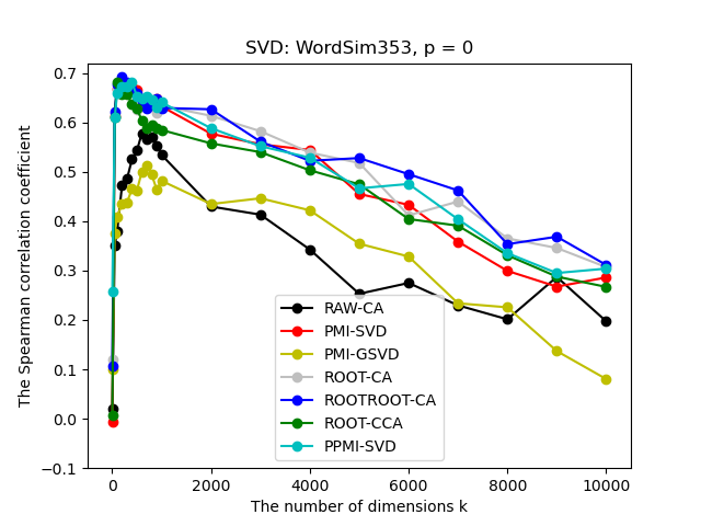
(a) WordSim353: $p=0$

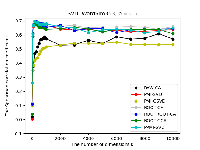
(b) WordSim353:$p=0.5$

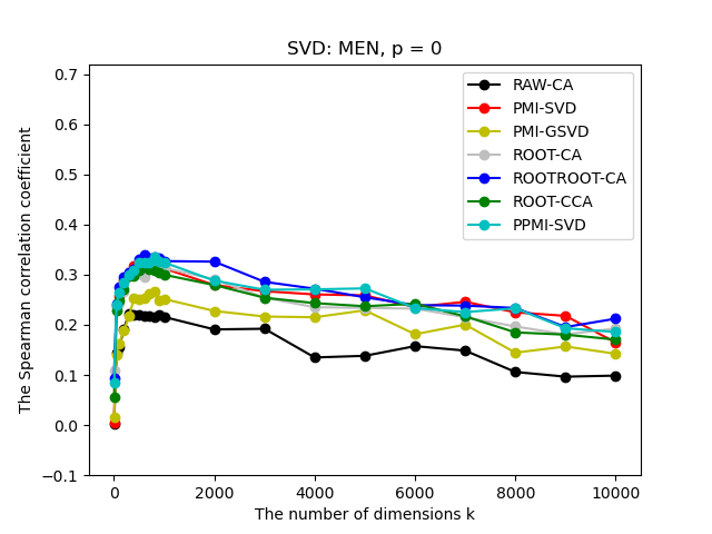
(c) MEN: $p=0$

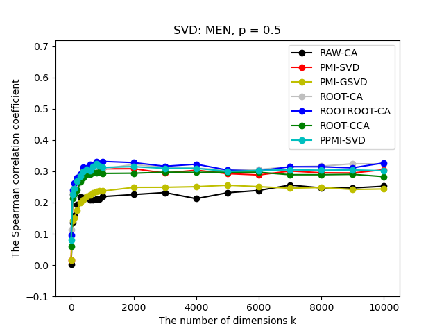
(d) MEN: $p=0.5$

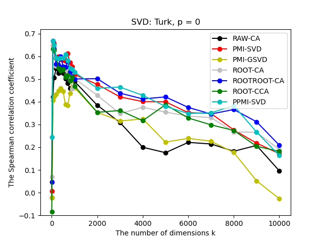
(e) Turk: $p=0$

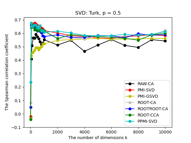
(f) Turk: $p=0.5$

Figure B.1: Text8

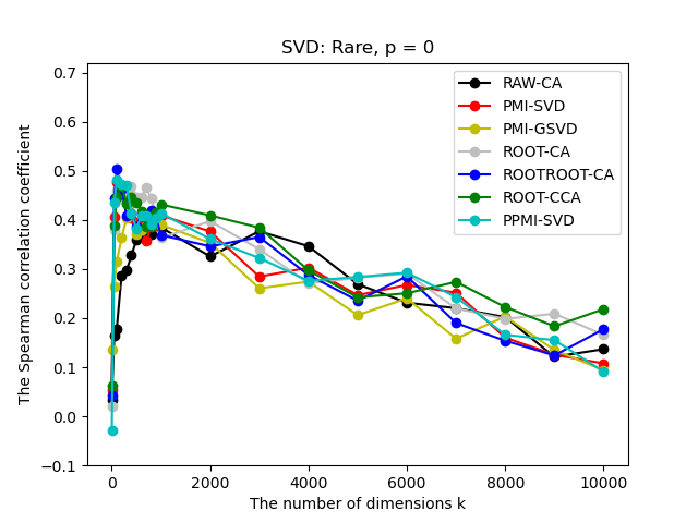
(a) Rare: $p=0$

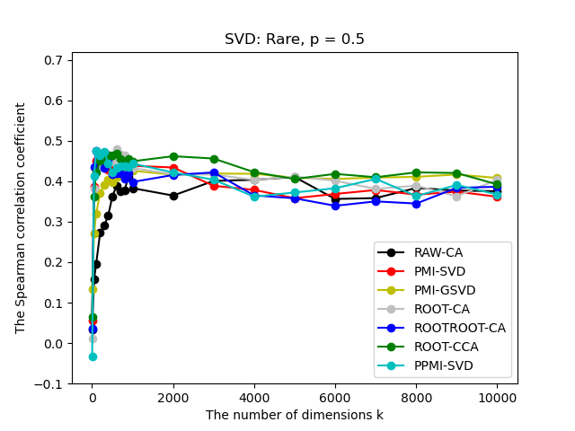
(b) Rare: $p=0.5$

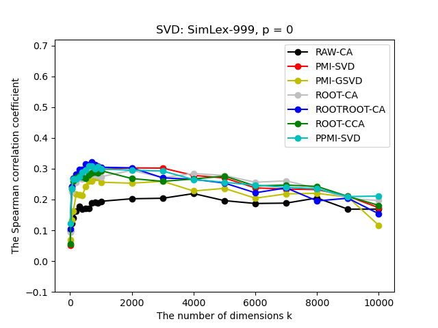
(c) SimLex-999: $p=0$

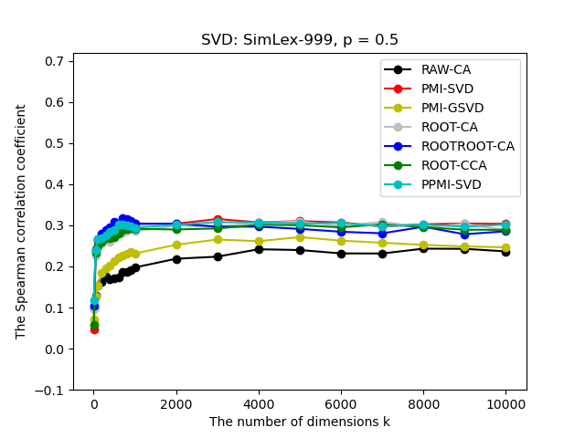
(d) SimLex-999: $p=0.5$

Figure B.2: Text8

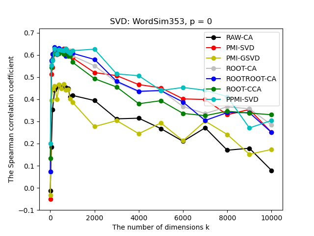
(a) WordSim353: $p=0$

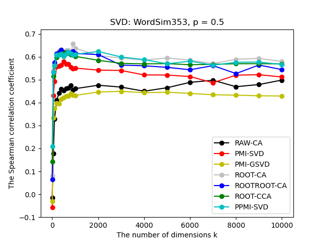
(b) WordSim353: $p=0.5$

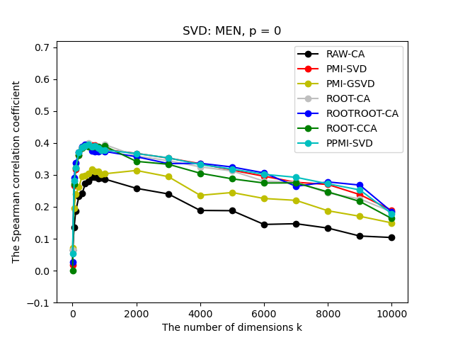
(c) MEN: $p=0$

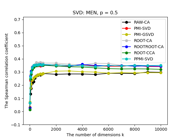
(d) MEN: $p=0.5$

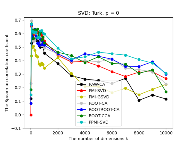
(e) Turk: $p=0$

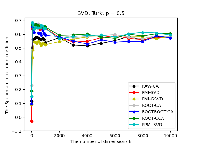
(f) Turk: $p=0.5$

Figure B.3: BNC

(a) Rare: $p=0$

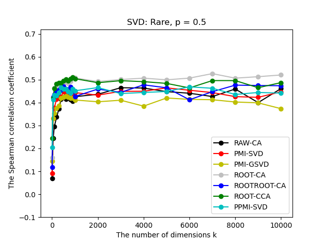
(b) Rare: $p=0.5$

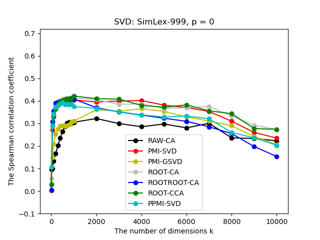
(c) SimLex-999: $p=0$

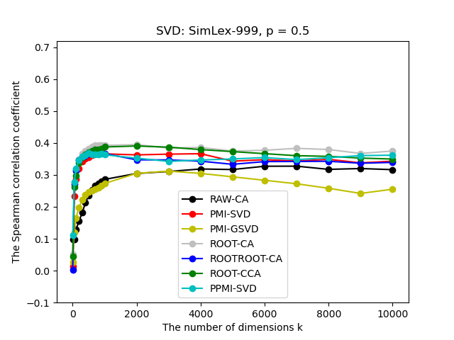
(d) SimLex-999: $p=0.5$

Figure B.4: BNC

Supplementary C: BNC: the number and sizes of extreme values of PMI, PPMI, and WPMI, and plots showing the contribution of the rows about PMI-SVD, PPMI-SVD, and PMI-GSVD

Table C.1, part PMI, PPMI, WPMI, shows the number of extreme values of PMI, PPMI, WPMI matrices. We only include non-zero pairs of PMI matrix because the PMI matrix is sparse: 84.1% of the entries are zero. The corresponding 84.1% of entries in PPMI and WPMI are also ignored. The number of extreme values of WPMI matrix (2,525,345) is much larger than that of PMI and PPMI (141,366 and 405,830). Furthermore, in WPMI the extremeness of the extreme values is much larger than those in PMI and PPMI. For example, where the average contribution of each cell is $1/\left(11,332\times 11,332\right)$, in WPMI the most extreme entry (the, the) contributes around 0.01150 to the total inertia, while in PMI (PPMI), the most extreme entry (ee, ee) contributes around $2.2\times 10^{-6}$ ($2.7\times 10^{-6}$) to the total inertia. Figure C.1 shows the contribution of the rows, corresponding to top 10 extreme values, to the first 100 dimensions of PMI-SVD, PPMI-SVD, PMI-GSVD. The rows, corresponding to the top extreme values of WPMI, take up a bigger contribution to the first dimensions of PMI-GSVD. For example, in PMI-GSVD, the “the” row contributes more than 0.3 to the third dimension, while in PMI-SVD and PPMI-SVD, the contributions are much smaller.

Table C.1: BNC: the number of extreme values

	LT$f_{1}$	GT$f_{3}$	total
PMI	13,982	127,384	141,366
PPMI	0	405,830	405,830
WPMI	2,037,800	487,545	2,525,345
TTEST	334,512	1,480,336	1,814,848
ROOT-TTEST	35,418	927,470	962,888
ROOTROOT-TTEST	31,234	750,433	781,667
STRATOS-TTEST	0	1,173,717	1,173,717

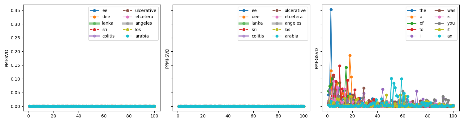
Figure C.1: BNC: the contribution of the rows, corresponding to top 10 extreme values, to first 100 dimensions of PMI-SVD, PPMI-SVD, PMI-GSVD.

Supplementary D: Text8: plots showing the contribution of the rows about ROOT-CCA

Figure D.1 shows the contribution of the rows, corresponding to top 10 extreme values, to first 100 dimensions of ROOT-CCA

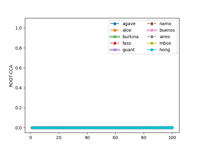
Figure D.1: Text8: the contribution of the rows, corresponding to top 10 extreme values, to first 100 dimensions of ROOT-CCA.

Supplementary E: BNC: the number and sizes of extreme values of TTEST, ROOT-TTEST, ROOTROOT-TTEST, and STRATOS-TTEST, and plots showing the contribution of the rows about RAW-CA, ROOT-CA, ROOTROOT-CA, and ROOT-CCA

The bottom part of Table C.1 shows the number of extreme values of TTEST, ROOT-TTEST, ROOTROOT-TTEST and STRATOS-TTEST matrices. Similar with PMI, PPMI, WPMI, 84.1% of entries are ignored. The number of extreme values of TTEST matrix (1,814,848) is much larger than that of ROOT-TTEST, ROOTROOT-TTEST and STRATOS-TTEST (962,888, 781,667, and 1,173,717). Furthermore, in TTEST the extremeness of the extreme values is much larger than in ROOT-TTEST, ROOTROOT-TTEST and STRATOS-TTEST. For example, in TTEST the most extreme entry (kong, hong) or (hong, kong) contributes around 0.00965 to the total inertia, while in ROOT-TTEST, ROOTROOT-TTEST and STRATOS-TTEST, the most extreme entries (colitis, ulcerative) or (ulcerative, colitis), (colitis, ulcerative) or (colitis, ulcerative), (hong, kong) or (kong, hong) contribute around 0.00047, 0.00003, and 0.00008 respectively. Figure E.1 shows the contribution of the rows, corresponding to top 10 extreme values, to first 100 dimensions of RAW-CA, ROOT-CA, and ROOTROOT-CA. The corresponding plot about ROOT-CCA is in Figure E.2. In RAW-CA, the rows, corresponding to top extreme values of TTEST, have a big contribution to the first dimensions of RAW-CA, while in ROOT-CA and ROOTROOT-CA, the contributions are much smaller, which also holds for ROOT-CCA.

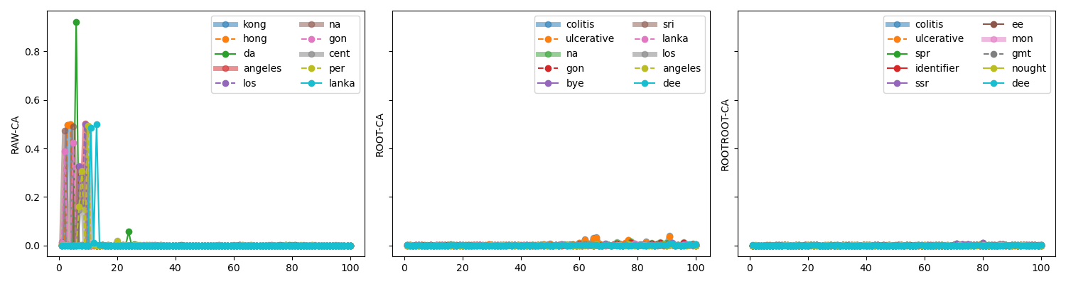
Figure E.1: BNC: the contribution of the rows, corresponding to top 10 extreme values, to first 100 dimensions of RAW-CA, ROOT-CA, ROOTROOT-CA.

Figure E.2: BNC: the contribution of the rows, corresponding to top 10 extreme values, to first 100 dimensions of ROOT-CCA.

References

- Agresti (\APACyear2007) \APACinsertmetastaragresti2007categorical{APACrefauthors}Agresti, A. \APACrefYear2007. \APACrefbtitleAn introduction to categorical data analysis An introduction to categorical data analysis. \APACaddressPublisherWiley. {APACrefDOI} 10.1002/0470114754 \PrintBackRefs\CurrentBib
- Alqahtani \BOthers. (\APACyear2023) \APACinsertmetastarALQAHTANI2023103338{APACrefauthors}Alqahtani, Y., Al-Twairesh, N.\BCBL \BBA Alsanad, A. \APACrefYearMonthDay2023. \BBOQ\APACrefatitleImproving sentiment domain adaptation for Arabic using an unsupervised self-labeling framework Improving sentiment domain adaptation for arabic using an unsupervised self-labeling framework.\BBCQ \APACjournalVolNumPagesInformation Processing & Management603103338. {APACrefDOI} 10.1016/j.ipm.2023.103338 \PrintBackRefs\CurrentBib
- Bae \BOthers. (\APACyear2021) \APACinsertmetastarbae2021keyword{APACrefauthors}Bae, Y\BPBIS., Kim, K\BPBIH., Kim, H\BPBIK., Choi, S\BPBIW., Ko, T., Seo, H\BPBIH.\BDBLJeon, H. \APACrefYearMonthDay2021. \BBOQ\APACrefatitleKeyword extraction algorithm for classifying smoking status from unstructured bilingual electronic health records based on natural language processing Keyword extraction algorithm for classifying smoking status from unstructured bilingual electronic health records based on natural language processing.\BBCQ \APACjournalVolNumPagesApplied Sciences11198812. {APACrefDOI} 10.3390/app11198812 \PrintBackRefs\CurrentBib
- Bartlett (\APACyear1936) \APACinsertmetastarbartlett1936square{APACrefauthors}Bartlett, M\BPBIS. \APACrefYearMonthDay1936. \BBOQ\APACrefatitleThe square root transformation in analysis of variance The square root transformation in analysis of variance.\BBCQ \APACjournalVolNumPagesSupplement to the Journal of the Royal Statistical Society3168–78. {APACrefDOI} 10.2307/2983678 \PrintBackRefs\CurrentBib
- Beh \BBA Lombardo (\APACyear2021) \APACinsertmetastarbeh2021introduction{APACrefauthors}Beh, E\BPBIJ.\BCBT \BBA Lombardo, R. \APACrefYear2021. \APACrefbtitleAn introduction to correspondence analysis An introduction to correspondence analysis. \APACaddressPublisherWiley. {APACrefDOI} 10.1002/9781119044482 \PrintBackRefs\CurrentBib
- Beh \BBA Lombardo (\APACyear2024) \APACinsertmetastarbeh2024correspondence{APACrefauthors}Beh, E\BPBIJ.\BCBT \BBA Lombardo, R. \APACrefYearMonthDay2024. \BBOQ\APACrefatitleCorrespondence analysis using the cressie–read family of divergence statistics Correspondence analysis using the cressie–read family of divergence statistics.\BBCQ \APACjournalVolNumPagesInternational Statistical Review92117–42. {APACrefDOI} 10.1111/insr.12541 \PrintBackRefs\CurrentBib
- Beh \BOthers. (\APACyear2018) \APACinsertmetastarbeh2018correspondence{APACrefauthors}Beh, E\BPBIJ., Lombardo, R.\BCBL \BBA Alberti, G. \APACrefYearMonthDay2018. \BBOQ\APACrefatitleCorrespondence analysis and the Freeman–Tukey statistic: A study of archaeological data Correspondence analysis and the freeman–tukey statistic: A study of archaeological data.\BBCQ \APACjournalVolNumPagesComputational Statistics & Data Analysis12873–86. {APACrefDOI} 10.1016/j.csda.2018.06.012 \PrintBackRefs\CurrentBib
- Beh \BOthers. (\APACyear2023) \APACinsertmetastarBeh2023{APACrefauthors}Beh, E\BPBIJ., Lombardo, R.\BCBL \BBA Wang, T\BHBIW. \APACrefYearMonthDay2023. \BBOQ\APACrefatitlePower Transformations and Reciprocal Averaging Power transformations and reciprocal averaging.\BBCQ \BIn E\BPBIJ. Beh, R. Lombardo\BCBL \BBA J\BPBIG. Clavel (\BEDS), \APACrefbtitleAnalysis of Categorical Data from Historical Perspectives: Essays in Honour of Shizuhiko Nishisato Analysis of categorical data from historical perspectives: Essays in honour of shizuhiko nishisato (\BPGS 173–199). \APACaddressPublisherSingaporeSpringer Nature Singapore. {APACrefDOI} 10.1007/978-981-99-5329-5_11 \PrintBackRefs\CurrentBib
- Benzécri (\APACyear1973) \APACinsertmetastarbenzecri1973analyse{APACrefauthors}Benzécri, J\BHBIP. \APACrefYear1973. \APACrefbtitleL’analyse des données L’analyse des données (\BVOL 1 and 2). \APACaddressPublisherDunod Paris. \PrintBackRefs\CurrentBib
- BNC Consortium (\APACyear2007) \APACinsertmetastarBNC{APACrefauthors}BNC Consortium. \APACrefYearMonthDay2007. \APACrefbtitleBritish National Corpus, XML edition. British National Corpus, XML edition. {APACrefURL} http://hdl.handle.net/20.500.14106/2554 \APACrefnoteLiterary and Linguistic Data Service \PrintBackRefs\CurrentBib
- Bruni \BOthers. (\APACyear2012) \APACinsertmetastarbruni2012distributional{APACrefauthors}Bruni, E., Boleda, G., Baroni, M.\BCBL \BBA Tran, N\BHBIK. \APACrefYearMonthDay2012. \BBOQ\APACrefatitleDistributional Semantics in Technicolor Distributional semantics in technicolor.\BBCQ \BIn \APACrefbtitleProceedings of the 50th Annual Meeting of the Association for Computational Linguistics (Volume 1: Long Papers) Proceedings of the 50th annual meeting of the association for computational linguistics (volume 1: Long papers) (\BPGS 136–145). {APACrefURL} https://aclanthology.org/P12-1015 \PrintBackRefs\CurrentBib
- Bullinaria \BBA Levy (\APACyear2007) \APACinsertmetastarbullinaria2007extracting{APACrefauthors}Bullinaria, J\BPBIA.\BCBT \BBA Levy, J\BPBIP. \APACrefYearMonthDay2007. \BBOQ\APACrefatitleExtracting semantic representations from word co-occurrence statistics: A computational study Extracting semantic representations from word co-occurrence statistics: A computational study.\BBCQ \APACjournalVolNumPagesBehavior Research Methods39510–526. {APACrefDOI} 10.3758/BF03193020 \PrintBackRefs\CurrentBib
- Cuadras \BBA Cuadras (\APACyear2006) \APACinsertmetastarCUADRAS200664{APACrefauthors}Cuadras, C\BPBIM.\BCBT \BBA Cuadras, D. \APACrefYearMonthDay2006. \BBOQ\APACrefatitleA parametric approach to correspondence analysis A parametric approach to correspondence analysis.\BBCQ \APACjournalVolNumPagesLinear Algebra and its Applications417164-74. \APACrefnoteSpecial Issue devoted to papers presented at the Workshop on Matrices and Statistics {APACrefDOI} https://doi.org/10.1016/j.laa.2005.10.029 \PrintBackRefs\CurrentBib
- Curran (\APACyear2004) \APACinsertmetastarcurran2004distributional{APACrefauthors}Curran, J\BPBIR. \APACrefYear2004. \APACrefbtitleFrom distributional to semantic similarity From distributional to semantic similarity \APACtypeAddressSchool\BPhDUniversity of Edinburgh. {APACrefURL} http://hdl.handle.net/1842/563 \PrintBackRefs\CurrentBib
- Curran \BBA Moens (\APACyear2002) \APACinsertmetastarcurran2002improvements{APACrefauthors}Curran, J\BPBIR.\BCBT \BBA Moens, M. \APACrefYearMonthDay2002. \BBOQ\APACrefatitleImprovements in Automatic Thesaurus Extraction Improvements in automatic thesaurus extraction.\BBCQ \BIn \APACrefbtitleProceedings of the ACL-02 Workshop on Unsupervised Lexical Acquisition - Volume 9 Proceedings of the ACL-02 Workshop on Unsupervised Lexical Acquisition - Volume 9 (\BPG 59–66). {APACrefDOI} 10.3115/1118627.1118635 \PrintBackRefs\CurrentBib
- Deerwester \BOthers. (\APACyear1990) \APACinsertmetastardeerwester1990indexing{APACrefauthors}Deerwester, S., Dumais, S\BPBIT., Furnas, G\BPBIW., Landauer, T\BPBIK.\BCBL \BBA Harshman, R. \APACrefYearMonthDay1990. \BBOQ\APACrefatitleIndexing by latent semantic analysis Indexing by latent semantic analysis.\BBCQ \APACjournalVolNumPagesJournal of the American society for information science416391–407. {APACrefDOI} 10.1002/(SICI)1097-4571(199009)41:6<391::AID-ASI1>3.0.CO;2-9 \PrintBackRefs\CurrentBib
- Dodge (\APACyear2008) \APACinsertmetastardodge2008concise{APACrefauthors}Dodge, Y. \APACrefYear2008. \APACrefbtitleThe Concise Encyclopedia of Statistics The concise encyclopedia of statistics. \APACaddressPublisherSpringer New York. {APACrefDOI} 10.1007/978-0-387-32833-1 \PrintBackRefs\CurrentBib
- Downing (\APACyear1981) \APACinsertmetastardowning1981well{APACrefauthors}Downing, J. \APACrefYearMonthDay1981. \BBOQ\APACrefatitleHOW WELL DOES THE 4TH-ROOT TRANSFORMATION WORK-REPLY How well does the 4th-root transformation work-reply.\BBCQ \APACjournalVolNumPagesCanadian Journal of Fisheries and Aquatic Sciences381127–129. \PrintBackRefs\CurrentBib
- Duchi \BOthers. (\APACyear2011) \APACinsertmetastarduchi2011adaptive{APACrefauthors}Duchi, J., Hazan, E.\BCBL \BBA Singer, Y. \APACrefYearMonthDay2011. \BBOQ\APACrefatitleAdaptive Subgradient Methods for Online Learning and Stochastic Optimization Adaptive subgradient methods for online learning and stochastic optimization.\BBCQ \APACjournalVolNumPagesJournal of machine learning research122121–2159. {APACrefURL} http://jmlr.org/papers/v12/duchi11a.html \PrintBackRefs\CurrentBib
- Dumais \BOthers. (\APACyear1988) \APACinsertmetastardumais1988using{APACrefauthors}Dumais, S\BPBIT., Furnas, G\BPBIW., Landauer, T\BPBIK., Deerwester, S.\BCBL \BBA Harshman, R. \APACrefYearMonthDay1988. \BBOQ\APACrefatitleUsing latent semantic analysis to improve access to textual information Using latent semantic analysis to improve access to textual information.\BBCQ \BIn \APACrefbtitleProceedings of the SIGCHI conference on Human factors in computing systems Proceedings of the SIGCHI conference on Human factors in computing systems (\BPGS 281–285). {APACrefDOI} 10.1145/57167.57214 \PrintBackRefs\CurrentBib
- Egleston \BOthers. (\APACyear2021) \APACinsertmetastaregleston2021statistical{APACrefauthors}Egleston, B\BPBIL., Bai, T., Bleicher, R\BPBIJ., Taylor, S\BPBIJ., Lutz, M\BPBIH.\BCBL \BBA Vucetic, S. \APACrefYearMonthDay2021. \BBOQ\APACrefatitleStatistical inference for natural language processing algorithms with a demonstration using type 2 diabetes prediction from electronic health record notes Statistical inference for natural language processing algorithms with a demonstration using type 2 diabetes prediction from electronic health record notes.\BBCQ \APACjournalVolNumPagesBiometrics7731089–1100. {APACrefDOI} 10.1111/biom.13338 \PrintBackRefs\CurrentBib
- Field \BOthers. (\APACyear1982) \APACinsertmetastarfield1982practical{APACrefauthors}Field, J., Clarke, K.\BCBL \BBA Warwick, R\BPBIM. \APACrefYearMonthDay1982. \BBOQ\APACrefatitleA practical strategy for analysing multispecies distribution patterns A practical strategy for analysing multispecies distribution patterns.\BBCQ \APACjournalVolNumPagesMarine ecology progress series8137–52. {APACrefURL} http://www.jstor.com/stable/24814621 \PrintBackRefs\CurrentBib
- Finkelstein \BOthers. (\APACyear2002) \APACinsertmetastarfinkelstein2002placing{APACrefauthors}Finkelstein, L., Gabrilovich, E., Matias, Y., Rivlin, E., Solan, Z., Wolfman, G.\BCBL \BBA Ruppin, E. \APACrefYearMonthDay2002. \BBOQ\APACrefatitlePlacing search in context: The concept revisited Placing search in context: The concept revisited.\BBCQ \APACjournalVolNumPagesACM Transactions on Information Systems201116–131. {APACrefDOI} 10.1145/503104.503110 \PrintBackRefs\CurrentBib
- France \BBA Heung (\APACyear2023) \APACinsertmetastarFRANCE2023100220{APACrefauthors}France, R\BPBIL.\BCBT \BBA Heung, B. \APACrefYearMonthDay2023. \BBOQ\APACrefatitleDensity variability of COVID-19 face mask litter: A cautionary tale for pandemic PPE waste monitoring Density variability of COVID-19 face mask litter: A cautionary tale for pandemic PPE waste monitoring.\BBCQ \APACjournalVolNumPagesJournal of Hazardous Materials Advances9100220. {APACrefDOI} 10.1016/j.hazadv.2022.100220 \PrintBackRefs\CurrentBib
- Goodman (\APACyear1996) \APACinsertmetastarLeo1996{APACrefauthors}Goodman, L\BPBIA. \APACrefYearMonthDay1996. \BBOQ\APACrefatitleA Single General Method for the Analysis of Cross-Classified Data: Reconciliation and Synthesis of Some Methods of Pearson, Yule, and Fisher, and Also Some Methods of Correspondence Analysis and Association Analysis A single general method for the analysis of cross-classified data: Reconciliation and synthesis of some methods of pearson, yule, and fisher, and also some methods of correspondence analysis and association analysis.\BBCQ \APACjournalVolNumPagesJournal of the American Statistical Association91433408–428. {APACrefDOI} 10.1080/01621459.1996.10476702 \PrintBackRefs\CurrentBib
- Greenacre (\APACyear1984) \APACinsertmetastargreenacre1984theory{APACrefauthors}Greenacre, M. \APACrefYear1984. \APACrefbtitleTheory and applications of correspondence analysis Theory and applications of correspondence analysis. \APACaddressPublisherAcademic Press. \PrintBackRefs\CurrentBib
- Greenacre (\APACyear2009) \APACinsertmetastargreenacre2009power{APACrefauthors}Greenacre, M. \APACrefYearMonthDay2009. \BBOQ\APACrefatitlePower transformations in correspondence analysis Power transformations in correspondence analysis.\BBCQ \APACjournalVolNumPagesComputational Statistics & Data Analysis5383107–3116. {APACrefDOI} 10.1016/j.csda.2008.09.001 \PrintBackRefs\CurrentBib
- Greenacre (\APACyear2010) \APACinsertmetastargreenacre2010log{APACrefauthors}Greenacre, M. \APACrefYearMonthDay2010. \BBOQ\APACrefatitleLog-ratio analysis is a limiting case of correspondence analysis Log-ratio analysis is a limiting case of correspondence analysis.\BBCQ \APACjournalVolNumPagesMathematical Geosciences42129–134. {APACrefDOI} 10.1007/s11004-008-9212-2 \PrintBackRefs\CurrentBib
- Greenacre (\APACyear2017) \APACinsertmetastargreenacre2017correspondence{APACrefauthors}Greenacre, M. \APACrefYear2017. \APACrefbtitleCorrespondence analysis in practice Correspondence analysis in practice. \APACaddressPublisherCRC press. {APACrefDOI} 10.1201/9781315369983 \PrintBackRefs\CurrentBib
- Greenacre \BBA Hastie (\APACyear1987) \APACinsertmetastargreenacre1987geometric{APACrefauthors}Greenacre, M.\BCBT \BBA Hastie, T. \APACrefYearMonthDay1987. \BBOQ\APACrefatitleThe geometric interpretation of correspondence analysis The geometric interpretation of correspondence analysis.\BBCQ \APACjournalVolNumPagesJournal of the American statistical association82398437–447. {APACrefDOI} 10.1080/01621459.1987.10478446 \PrintBackRefs\CurrentBib
- Guo \BBA Yao (\APACyear2021) \APACinsertmetastarguo2021document{APACrefauthors}Guo, S.\BCBT \BBA Yao, N. \APACrefYearMonthDay2021. \BBOQ\APACrefatitleDocument Vector Extension for Documents Classification Document vector extension for documents classification.\BBCQ \APACjournalVolNumPagesIEEE Transactions on Knowledge & Data Engineering3383062–3074. {APACrefDOI} 10.1109/TKDE.2019.2961343 \PrintBackRefs\CurrentBib
- Hill \BOthers. (\APACyear2015) \APACinsertmetastarhill-etal-2015-simlex{APACrefauthors}Hill, F., Reichart, R.\BCBL \BBA Korhonen, A. \APACrefYearMonthDay2015. \BBOQ\APACrefatitleSimLex-999: Evaluating Semantic Models With (Genuine) Similarity Estimation SimLex-999: Evaluating Semantic Models With (Genuine) Similarity Estimation.\BBCQ \APACjournalVolNumPagesComputational Linguistics414665–695. {APACrefDOI} 10.1162/COLI_a_00237 \PrintBackRefs\CurrentBib
- Hollander \BOthers. (\APACyear2013) \APACinsertmetastarhollander2013nonparametric{APACrefauthors}Hollander, M., Wolfe, D\BPBIA.\BCBL \BBA Chicken, E. \APACrefYear2013. \APACrefbtitleNonparametric statistical methods Nonparametric statistical methods. \APACaddressPublisherJohn Wiley & Sons. \PrintBackRefs\CurrentBib
- Hsu \BBA Culhane (\APACyear2023) \APACinsertmetastarhsu2023correspondence{APACrefauthors}Hsu, L\BPBIL.\BCBT \BBA Culhane, A\BPBIC. \APACrefYearMonthDay2023. \BBOQ\APACrefatitleCorrespondence analysis for dimension reduction, batch integration, and visualization of single-cell RNA-seq data Correspondence analysis for dimension reduction, batch integration, and visualization of single-cell RNA-seq data.\BBCQ \APACjournalVolNumPagesScientific Reports131197. {APACrefDOI} 10.1038/s41598-022-26434-1 \PrintBackRefs\CurrentBib
- Jiang \BOthers. (\APACyear2018) \APACinsertmetastarjiang-etal-2018-learning{APACrefauthors}Jiang, C., Yu, H\BHBIF., Hsieh, C\BHBIJ.\BCBL \BBA Chang, K\BHBIW. \APACrefYearMonthDay2018. \BBOQ\APACrefatitleLearning Word Embeddings for Low-Resource Languages by PU Learning Learning word embeddings for low-resource languages by PU learning.\BBCQ \BIn \APACrefbtitleProceedings of the 2018 Conference of the North American Chapter of the Association for Computational Linguistics: Human Language Technologies, Volume 1 (Long Papers) Proceedings of the 2018 conference of the north American chapter of the association for computational linguistics: Human language technologies, volume 1 (long papers) (\BPGS 1024–1034). {APACrefDOI} 10.18653/v1/N18-1093 \PrintBackRefs\CurrentBib
- Jurafsky \BBA Martin (\APACyear2023) \APACinsertmetastarjurafsky2023vector{APACrefauthors}Jurafsky, D.\BCBT \BBA Martin, J\BPBIH. \APACrefYearMonthDay2023. \BBOQ\APACrefatitleVector semantics and embeddings Vector semantics and embeddings.\BBCQ \APACjournalVolNumPagesSpeech and language processing1–34. \APAChowpublishedRetrieved December 21, 2023, from https://web.stanford.edu/~jurafsky/slp3/6.pdf. \PrintBackRefs\CurrentBib
- Kostensalo \BOthers. (\APACyear2023) \APACinsertmetastarKOSTENSALO2023100912{APACrefauthors}Kostensalo, J., Lidauer, M., Aernouts, B., Mäntysaari, P., Kokkonen, T., Lidauer, P.\BCBL \BBA Mehtiö, T. \APACrefYearMonthDay2023. \BBOQ\APACrefatitleShort communication: Predicting blood plasma non-esterified fatty acid and beta-hydroxybutyrate concentrations from cow milk—addressing systematic issues in modelling Short communication: Predicting blood plasma non-esterified fatty acid and beta-hydroxybutyrate concentrations from cow milk—addressing systematic issues in modelling.\BBCQ \APACjournalVolNumPagesanimal179100912. {APACrefDOI} 10.1016/j.animal.2023.100912 \PrintBackRefs\CurrentBib
- Levy \BBA Goldberg (\APACyear2014) \APACinsertmetastarlevy2014neural{APACrefauthors}Levy, O.\BCBT \BBA Goldberg, Y. \APACrefYearMonthDay2014. \BBOQ\APACrefatitleNeural Word Embedding as Implicit Matrix Factorization Neural word embedding as implicit matrix factorization.\BBCQ \BIn \APACrefbtitleAdvances in Neural Information Processing Systems Advances in neural information processing systems (\BVOL 27). {APACrefURL} https://proceedings.neurips.cc/paper_files/paper/2014/file/feab05aa91085b7a8012516bc3533958-Paper.pdf \PrintBackRefs\CurrentBib
- Levy \BOthers. (\APACyear2015) \APACinsertmetastarlevy2015improving{APACrefauthors}Levy, O., Goldberg, Y.\BCBL \BBA Dagan, I. \APACrefYearMonthDay2015. \BBOQ\APACrefatitleImproving Distributional Similarity with Lessons Learned from Word Embeddings Improving distributional similarity with lessons learned from word embeddings.\BBCQ \APACjournalVolNumPagesTransactions of the Association for Computational Linguistics3211–225. {APACrefDOI} 10.1162/tacl_a_00134 \PrintBackRefs\CurrentBib
- Luong \BOthers. (\APACyear2013) \APACinsertmetastarluong2013better{APACrefauthors}Luong, T., Socher, R.\BCBL \BBA Manning, C. \APACrefYearMonthDay2013. \BBOQ\APACrefatitleBetter Word Representations with Recursive Neural Networks for Morphology Better word representations with recursive neural networks for morphology.\BBCQ \BIn \APACrefbtitleProceedings of the Seventeenth Conference on Computational Natural Language Learning Proceedings of the seventeenth conference on computational natural language learning (\BPGS 104–113). {APACrefURL} https://aclanthology.org/W13-3512 \PrintBackRefs\CurrentBib
- Mikolov, Chen\BCBL \BOthers. (\APACyear2013) \APACinsertmetastarmikolov2013efficient{APACrefauthors}Mikolov, T., Chen, K., Corrado, G.\BCBL \BBA Dean, J. \APACrefYearMonthDay2013. \BBOQ\APACrefatitleEfficient estimation of word representations in vector space Efficient estimation of word representations in vector space.\BBCQ \BIn \APACrefbtitleProceedings of the international conference on Learning Representations ICLR’13. Proceedings of the international conference on Learning Representations ICLR’13. \PrintBackRefs\CurrentBib
- Mikolov, Sutskever\BCBL \BOthers. (\APACyear2013) \APACinsertmetastarmikolov2013distributed{APACrefauthors}Mikolov, T., Sutskever, I., Chen, K., Corrado, G\BPBIS.\BCBL \BBA Dean, J. \APACrefYearMonthDay2013. \BBOQ\APACrefatitleDistributed Representations of Words and Phrases and their Compositionality Distributed representations of words and phrases and their compositionality.\BBCQ \BIn \APACrefbtitleAdvances in Neural Information Processing Systems Advances in neural information processing systems (\BVOL 26). {APACrefURL} https://proceedings.neurips.cc/paper_files/paper/2013/file/9aa42b31882ec039965f3c4923ce901b-Paper.pdf \PrintBackRefs\CurrentBib
- Nishisato \BOthers. (\APACyear2021) \APACinsertmetastarNishisato2021{APACrefauthors}Nishisato, S., Beh, E\BPBIJ., Lombardo, R.\BCBL \BBA Clavel, J\BPBIG. \APACrefYearMonthDay2021. \BBOQ\APACrefatitleOn the Analysis of Over-Dispersed Categorical Data On the analysis of over-dispersed categorical data.\BBCQ \BIn \APACrefbtitleModern Quantification Theory: Joint Graphical Display, Biplots, and Alternatives Modern quantification theory: Joint graphical display, biplots, and alternatives (\BPGS 215–231). \APACaddressPublisherSpringer Singapore. {APACrefDOI} 10.1007/978-981-16-2470-4_11 \PrintBackRefs\CurrentBib
- Pakzad \BBA Analoui (\APACyear2021) \APACinsertmetastarpakzad2021word{APACrefauthors}Pakzad, A.\BCBT \BBA Analoui, M. \APACrefYearMonthDay2021. \BBOQ\APACrefatitleA Word Selection Method for Producing Interpretable Distributional Semantic Word Vectors A word selection method for producing interpretable distributional semantic word vectors.\BBCQ \APACjournalVolNumPagesJournal of Artificial Intelligence Research721281–1305. {APACrefDOI} 10.1613/jair.1.13353 \PrintBackRefs\CurrentBib
- Peng \BBA Feldman (\APACyear2017) \APACinsertmetastarpeng2017automatic{APACrefauthors}Peng, J.\BCBT \BBA Feldman, A. \APACrefYearMonthDay2017. \BBOQ\APACrefatitleAutomatic Idiom Recognition with Word Embeddings Automatic idiom recognition with word embeddings.\BBCQ \BIn \APACrefbtitleInformation Management and Big Data Information management and big data (\BPGS 17–29). \APACaddressPublisherChamSpringer International Publishing. {APACrefDOI} 10.1007/978-3-319-55209-5_2 \PrintBackRefs\CurrentBib
- Pennington \BOthers. (\APACyear2014) \APACinsertmetastarpennington2014glove{APACrefauthors}Pennington, J., Socher, R.\BCBL \BBA Manning, C. \APACrefYearMonthDay2014. \BBOQ\APACrefatitleGloVe: Global Vectors for Word Representation GloVe: Global Vectors for Word Representation.\BBCQ \BIn \APACrefbtitleProceedings of the 2014 Conference on Empirical Methods in Natural Language Processing (EMNLP) Proceedings of the 2014 conference on empirical methods in natural language processing (EMNLP) (\BPGS 1532–1543). {APACrefDOI} 10.3115/v1/D14-1162 \PrintBackRefs\CurrentBib
- Podkorytov \BOthers. (\APACyear2020) \APACinsertmetastarpodkorytov2020effects{APACrefauthors}Podkorytov, M., Biś, D., Cai, J., Amirizirtol, K.\BCBL \BBA Liu, X. \APACrefYearMonthDay2020. \BBOQ\APACrefatitleEffects of Architecture and Training on Embedding Geometry and Feature Discriminability in BERT Effects of Architecture and Training on Embedding Geometry and Feature Discriminability in BERT.\BBCQ \BIn \APACrefbtitle2020 International Joint Conference on Neural Networks (IJCNN) 2020 International Joint Conference on Neural Networks (IJCNN) (\BPG 1-8). {APACrefDOI} 10.1109/IJCNN48605.2020.9206645 \PrintBackRefs\CurrentBib
- Qi, Hessen, Deoskar\BCBL \BBA Van der Heijden (\APACyear2023) \APACinsertmetastarqi2021comparison{APACrefauthors}Qi, Q., Hessen, D\BPBIJ., Deoskar, T.\BCBL \BBA Van der Heijden, P\BPBIG\BPBIM. \APACrefYearMonthDay2023. \BBOQ\APACrefatitleA comparison of latent semantic analysis and correspondence analysis of document-term matrices A comparison of latent semantic analysis and correspondence analysis of document-term matrices.\BBCQ \APACjournalVolNumPagesNatural Language Engineering1–31. {APACrefDOI} 10.1017/S1351324923000244 \PrintBackRefs\CurrentBib
- Qi, Hessen\BCBL \BBA Van der Heijden (\APACyear2023) \APACinsertmetastarqi2023improving{APACrefauthors}Qi, Q., Hessen, D\BPBIJ.\BCBL \BBA Van der Heijden, P\BPBIG\BPBIM. \APACrefYearMonthDay2023. \BBOQ\APACrefatitleImproving information retrieval through correspondence analysis instead of latent semantic analysis Improving information retrieval through correspondence analysis instead of latent semantic analysis.\BBCQ \APACjournalVolNumPagesJournal of Intelligent Information Systems. {APACrefDOI} 10.1007/s10844-023-00815-y \PrintBackRefs\CurrentBib
- Radinsky \BOthers. (\APACyear2011) \APACinsertmetastarradinsky2011word{APACrefauthors}Radinsky, K., Agichtein, E., Gabrilovich, E.\BCBL \BBA Markovitch, S. \APACrefYearMonthDay2011. \BBOQ\APACrefatitleA Word at a Time: Computing Word Relatedness Using Temporal Semantic Analysis A word at a time: Computing word relatedness using temporal semantic analysis.\BBCQ \BIn \APACrefbtitleProceedings of the 20th International Conference on World Wide Web Proceedings of the 20th international conference on world wide web (\BPG 337–346). {APACrefDOI} 10.1145/1963405.1963455 \PrintBackRefs\CurrentBib
- Raphael (\APACyear2023) \APACinsertmetastarraphael2023gendered{APACrefauthors}Raphael, E\BPBIB. \APACrefYearMonthDay2023. \BBOQ\APACrefatitleGendered Representations in Language: A Corpus-Based Comparative Study of Adjective-Noun Collocations for Marital Relationships Gendered representations in language: A corpus-based comparative study of adjective-noun collocations for marital relationships.\BBCQ \APACjournalVolNumPagesTheory and Practice in Language Studies1351191–1196. {APACrefDOI} 10.17507/tpls.1305.12 \PrintBackRefs\CurrentBib
- Roesler \BOthers. (\APACyear2019) \APACinsertmetastarroesler2019evaluation{APACrefauthors}Roesler, O., Aly, A., Taniguchi, T.\BCBL \BBA Hayashi, Y. \APACrefYearMonthDay2019. \BBOQ\APACrefatitleEvaluation of Word Representations in Grounding Natural Language Instructions Through Computational Human-Robot Interaction Evaluation of Word Representations in Grounding Natural Language Instructions Through Computational Human-Robot Interaction.\BBCQ \BIn \APACrefbtitle2019 14th ACM/IEEE International Conference on Human-Robot Interaction (HRI) 2019 14th ACM/IEEE International Conference on Human-Robot Interaction (HRI) (\BPG 307-316). {APACrefDOI} 10.1109/HRI.2019.8673121 \PrintBackRefs\CurrentBib
- Rong (\APACyear2014) \APACinsertmetastarrong2014word2vec{APACrefauthors}Rong, X. \APACrefYearMonthDay2014. \BBOQ\APACrefatitleword2vec parameter learning explained word2vec parameter learning explained.\BBCQ \APACjournalVolNumPagesarXiv preprint arXiv:1411.2738. \PrintBackRefs\CurrentBib
- Rumelhart \BOthers. (\APACyear1986) \APACinsertmetastarrumelhart1986learning{APACrefauthors}Rumelhart, D\BPBIE., Hinton, G\BPBIE.\BCBL \BBA Williams, R\BPBIJ. \APACrefYearMonthDay1986. \BBOQ\APACrefatitleLearning representations by back-propagating errors Learning representations by back-propagating errors.\BBCQ \APACjournalVolNumPagesnature3236088533–536. {APACrefDOI} 10.1038/323533a0 \PrintBackRefs\CurrentBib
- Salle \BBA Villavicencio (\APACyear2023) \APACinsertmetastarsalle2022understanding{APACrefauthors}Salle, A.\BCBT \BBA Villavicencio, A. \APACrefYearMonthDay2023. \BBOQ\APACrefatitleUnderstanding the effects of negative (and positive) pointwise mutual information on word vectors Understanding the effects of negative (and positive) pointwise mutual information on word vectors.\BBCQ \APACjournalVolNumPagesJournal of Experimental & Theoretical Artificial Intelligence3581161-1199. {APACrefDOI} 10.1080/0952813X.2022.2072004 \PrintBackRefs\CurrentBib
- Salle \BOthers. (\APACyear2016) \APACinsertmetastarsalle2016matrix{APACrefauthors}Salle, A., Villavicencio, A.\BCBL \BBA Idiart, M. \APACrefYearMonthDay2016. \BBOQ\APACrefatitleMatrix Factorization using Window Sampling and Negative Sampling for Improved Word Representations Matrix factorization using window sampling and negative sampling for improved word representations.\BBCQ \BIn \APACrefbtitleProceedings of the 54th Annual Meeting of the Association for Computational Linguistics (Volume 2: Short Papers) Proceedings of the 54th annual meeting of the association for computational linguistics (volume 2: Short papers) (\BPGS 419–424). {APACrefDOI} 10.18653/v1/P16-2068 \PrintBackRefs\CurrentBib
- Samuel \BOthers. (\APACyear2023) \APACinsertmetastarsamuel-etal-2023-trained{APACrefauthors}Samuel, D., Kutuzov, A., Øvrelid, L.\BCBL \BBA Velldal, E. \APACrefYearMonthDay2023. \BBOQ\APACrefatitleTrained on 100 million words and still in shape: BERT meets British National Corpus Trained on 100 million words and still in shape: BERT meets British National Corpus.\BBCQ \BIn \APACrefbtitleFindings of the Association for Computational Linguistics: EACL 2023 Findings of the Association for Computational Linguistics: EACL 2023 (\BPGS 1954–1974). {APACrefDOI} 10.18653/v1/2023.findings-eacl.146 \PrintBackRefs\CurrentBib
- Sasaki \BOthers. (\APACyear2023) \APACinsertmetastarsasaki2023examining{APACrefauthors}Sasaki, S., Heinzerling, B., Suzuki, J.\BCBL \BBA Inui, K. \APACrefYearMonthDay2023. \BBOQ\APACrefatitleExamining the effect of whitening on static and contextualized word embeddings Examining the effect of whitening on static and contextualized word embeddings.\BBCQ \APACjournalVolNumPagesInformation Processing & Management603103272. {APACrefDOI} 10.1016/j.ipm.2023.103272 \PrintBackRefs\CurrentBib
- Schwertman \BOthers. (\APACyear2004) \APACinsertmetastarschwertman2004simple{APACrefauthors}Schwertman, N\BPBIC., Owens, M\BPBIA.\BCBL \BBA Adnan, R. \APACrefYearMonthDay2004. \BBOQ\APACrefatitleA simple more general boxplot method for identifying outliers A simple more general boxplot method for identifying outliers.\BBCQ \APACjournalVolNumPagesComputational Statistics & Data Analysis471165-174. {APACrefDOI} 10.1016/j.csda.2003.10.012 \PrintBackRefs\CurrentBib
- Shazeer \BOthers. (\APACyear2016) \APACinsertmetastarshazeer2016swivel{APACrefauthors}Shazeer, N., Doherty, R., Evans, C.\BCBL \BBA Waterson, C. \APACrefYearMonthDay2016. \BBOQ\APACrefatitleSwivel: Improving embeddings by noticing what’s missing Swivel: Improving embeddings by noticing what’s missing.\BBCQ \APACjournalVolNumPagesarXiv preprint arXiv:1602.02215. \PrintBackRefs\CurrentBib
- Shi \BBA Liu (\APACyear2014) \APACinsertmetastarshi2014linking{APACrefauthors}Shi, T.\BCBT \BBA Liu, Z. \APACrefYearMonthDay2014. \BBOQ\APACrefatitleLinking GloVe with word2vec Linking glove with word2vec.\BBCQ \APACjournalVolNumPagesarXiv preprint arXiv:1411.5595. \PrintBackRefs\CurrentBib
- Stratos \BOthers. (\APACyear2015) \APACinsertmetastarstratos2015model{APACrefauthors}Stratos, K., Collins, M.\BCBL \BBA Hsu, D. \APACrefYearMonthDay2015. \BBOQ\APACrefatitleModel-based Word Embeddings from Decompositions of Count Matrices Model-based word embeddings from decompositions of count matrices.\BBCQ \BIn \APACrefbtitleProceedings of the 53rd Annual Meeting of the Association for Computational Linguistics and the 7th International Joint Conference on Natural Language Processing (Volume 1: Long Papers) Proceedings of the 53rd annual meeting of the association for computational linguistics and the 7th international joint conference on natural language processing (volume 1: Long papers) (\BPGS 1282–1291). {APACrefDOI} 10.3115/v1/P15-1124 \PrintBackRefs\CurrentBib
- \APACcitebtitleText8 dataset (\APACyear2006) \APACinsertmetastartext8\APACrefbtitleText8 dataset. Text8 dataset. \APACrefYearMonthDay2006. \APAChowpublishedRetrieved October 3, 2023, from http://mattmahoney.net/dc/text8.zip. \PrintBackRefs\CurrentBib
- Tukey (\APACyear1977) \APACinsertmetastartukey1977exploratory{APACrefauthors}Tukey, J\BPBIW. \APACrefYear1977. \APACrefbtitleExploratory data analysis Exploratory data analysis. \APACaddressPublisherAddison-Wesley, Reading, MA. \PrintBackRefs\CurrentBib
- Turney \BBA Pantel (\APACyear2010) \APACinsertmetastarturney2010frequency{APACrefauthors}Turney, P\BPBID.\BCBT \BBA Pantel, P. \APACrefYearMonthDay2010. \BBOQ\APACrefatitleFrom frequency to meaning: Vector space models of semantics From frequency to meaning: Vector space models of semantics.\BBCQ \APACjournalVolNumPagesJournal of artificial intelligence research37141–188. {APACrefDOI} 10.1613/jair.2934 \PrintBackRefs\CurrentBib
- Van der Heijden \BOthers. (\APACyear1989) \APACinsertmetastarvan1989combined{APACrefauthors}Van der Heijden, P\BPBIG\BPBIM., De Falguerolles, A.\BCBL \BBA De Leeuw, J. \APACrefYearMonthDay1989. \BBOQ\APACrefatitleA combined approach to contingency table analysis using correspondence analysis and loglinear analysis A combined approach to contingency table analysis using correspondence analysis and loglinear analysis.\BBCQ \APACjournalVolNumPagesJournal of the Royal Statistical Society: Series C (Applied Statistics)382249–292. {APACrefDOI} 10.2307/2348058 \PrintBackRefs\CurrentBib
- Xin \BOthers. (\APACyear2018) \APACinsertmetastarxin2018batch{APACrefauthors}Xin, X., Yuan, F., He, X.\BCBL \BBA Jose, J\BPBIM. \APACrefYearMonthDay2018. \BBOQ\APACrefatitleBatch IS NOT Heavy: Learning Word Representations From All Samples Batch IS NOT heavy: Learning word representations from all samples.\BBCQ \BIn \APACrefbtitleProceedings of the 56th Annual Meeting of the Association for Computational Linguistics (Volume 1: Long Papers) Proceedings of the 56th annual meeting of the association for computational linguistics (volume 1: Long papers) (\BPGS 1853–1862). {APACrefDOI} 10.18653/v1/P18-1172 \PrintBackRefs\CurrentBib
- Zhang \BOthers. (\APACyear2022) \APACinsertmetastarzhang2022word{APACrefauthors}Zhang, M., Palade, V., Wang, Y.\BCBL \BBA Ji, Z. \APACrefYearMonthDay2022. \BBOQ\APACrefatitleWord representation using refined contexts Word representation using refined contexts.\BBCQ \APACjournalVolNumPagesApplied Intelligence5212347–12368. {APACrefDOI} 10.1007/s10489-021-02898-y \PrintBackRefs\CurrentBib