Flow matching achieves minimax optimal convergence

Abstract

Flow matching (FM) has gained significant attention as a simulation-free generative model. Unlike diffusion models, which are based on stochastic differential equations, FM employs a simpler approach by solving an ordinary differential equation with an initial condition from a normal distribution, thus streamlining the sample generation process. This paper discusses the convergence properties of FM in terms of the $p$-Wasserstein distance, a measure of distributional discrepancy. We establish that FM can achieve the minmax optimal convergence rate for $1\leq p\leq 2$, presenting the first theoretical evidence that FM can reach convergence rates comparable to those of diffusion models. Our analysis extends existing frameworks by examining a broader class of mean and variance functions for the vector fields and identifies specific conditions necessary to attain these optimal rates.

1 Introduction

Flow matching (FM) [16] is a recent simulation-free generative model that produces samples by solving an ordinary differential equation initialized with a normal distribution. The approach bypasses the computationally intensive Monte-Carlo sampling required by the diffusion model, currently the standard in generative modeling. In addition to Lipman et al. [16], several variations have been proposed to refine the learning of vector fields, such as OT-CFM [27] and Rectified flow [18]. A series of studies also emerge from the viewpoint of interpolating distributions [2, 1].

Flow matching has already been applied to various domains with promising performance. Among many others, the rectified flow method has been extended to high-resolution text-image generation [8]; there are also many works on the application of FM to molecule generation [10, 9, 5, 7], as well as text generation [11], speech generation [15], motion synthesis [12], and point cloud generation [28].

Although the methods have been developed on the basis of the theory of the flows and continuity equations, their statistical behaviors remain less understood. Recent works have established the convergence of the FM estimator to the true distribution under some distributional metrics [2, 4]. Beyond the convergence, more detailed understandings, such as convergence rates, are still an open question. To contrast, diffusion models have gained various theoretical understandings, including the convergence rate in terms of the number of steps [6, 3] as well as the sample size [21, 29]. Among others, [21] has shown that diffusion models achieve the minmax optimal convergence rate for a large sample size in terms of 1-Wasserstein distance and total variation, which supports the high generation ability of diffusion models theoretically.

This paper aims to bridge this gap by demonstrating that FM can achieve the minmax optimal convergence rate for a large sample size under the $p$-Wasserstein distance for $1\leq p\leq 2$, suggesting that FM has a theoretical ability comparable to diffusion models. This question is important to understand the merits of flow matching and to reveal the difference between SDE and ODE in the generation of models. Drawing on the methodologies of Oko et al. [21], our analysis not only extends to a broader class of mean and variance functions of the normal distributions for conditional vector fields, but also specifies the conditions on these parameters under which optimal rate can be derived.

The contributions of this paper are as follows.

• We establish that a widely used class of conditional FM methods achieves the minmax optimal convergence rate under the $p$-Wasserstein distance ($1\leq p\leq 2$), marking the first theoretical demonstration of such performance of FM.

• We provide an analytical derivation of the upper bounds of the convergence rate under various settings of the mean and variance parameters.

• We reveal that the variance parameter must be decreased around the target distribution at some specific rate to attain the minmax optimality.

2 Preliminaries

2.1 Review of flow matching

This section provides a general review of FM, following [16, 27]. The aim of FM is to generate samples from the unknown true probability $P_{true}$, when training data $\{{\bm{x}}^{i}\}_{i=1}^{n}\subset{\mathbb{R}}^{d}$ of size $n$ is given as an i.i.d. sample from $P_{true}$. FM methods realize it by a flow that transports the standard normal distribution to the true distribution $P_{true}$ or its approximation. The flow is obtained as a solution to the ordinary differential equation (ODE) given by a desired vector field learned from the training data. A sample is generated by solving the ODE numerically with an initial point from the standard normal distribution.

More specifically, the (conditional) FM method [16] produces simple random vectors used for teaching data along paths, giving the desired vector field by average. Taking a sample ${\bm{y}}$ from the empirical distribution $\hat{P}_{train}$ of the training data, the method gives a point ${\bm{x}}_{(s)}$ ($s\in[0,1])$ based on the conditional normal distribution $P_{(s)}({\bm{x}}_{(s)}|{\bm{y}})=N(\mu_{(s)}({\bm{y}}),\sigma_{(s)}({\bm{y}})I_{d})$, and assigns a vector ${\bm{v}}_{(s)}({\bm{x}}_{(s)}|{\bm{y}})$ at $({\bm{x}}_{(s)},s)\in{\mathbb{R}}^{d}\times[0,1]$. The time $s$ is typically uniformly sampled. The vector ${\bm{v}}_{(s)}({\bm{x}}_{(s)}|{\bm{y}})$ is made so that it satisfies the following conditional continuity equation:

$$\frac{\partial}{\partial s}p_{(s)}({\bm{x}}_{(s)}|{\bm{y}})+{\rm div}\left(p_{(s)}({\bm{x}}_{(s)}|{\bm{y}}){\bm{v}}_{(s)}({\bm{x}}_{(s)}|{\bm{y}})\right)=0.$$ (1)

A typical construction [16] is given by

$$\mu_{(s)}({\bm{y}})=m_{(s)}{\bm{y}},\quad\sigma_{(s)}({\bm{y}})=\sigma_{(s)},$$

$${\bm{v}}_{(s)}({\bm{x}}|{\bm{y}})=\sigma^{\prime}_{(s)}\frac{{\bm{x}}-m_{(s)}{\bm{y}}}{\sigma_{(s)}}+m^{\prime}_{(s)}{\bm{y}},$$ (2)

where $m_{(s)}$ and $\sigma_{(s)}$ depend only on $s$, and $m_{(s)}^{\prime}$ and $\sigma_{(s)}^{\prime}$ denote the derivatives with respect to $s$. It is easy to see that (2) satisfies the conditional continuity equation (1). The mean $m_{(s)}$ and variance $\sigma_{(s)}$ are increasing and increasing function of $s$, respectively, such that

$$m_{(s)}\to 1\text{\;\;for\;\;}s\to 1,\qquad m_{(s)}\to 0\text{\;\;for\;\;}s\to+0,$$

$$\sigma_{(s)}\to 0\text{\;\;for\;\;}s\to 1,\qquad\sigma_{(s)}\to 1\text{ for }s\to+0.$$

Note that, given location $({\bm{x}},s)$, the vector ${\bm{v}}_{(s)}({\bm{x}}|{\bm{y}})$ is random depending on the randomness of ${\bm{y}}$; Different vectors may be assigned to the same location. It is easy to see that, by taking average over ${\bm{y}}\sim P_{true}$, the distribution of ${\bm{x}}$

$$p_{(s)}({\bm{x}})={\textstyle\int}p_{(s)}({\bm{x}}|{\bm{y}})dP_{true}({\bm{y}})$$ (3)

satisfies the continuity equation

$$\frac{\partial}{\partial s}p_{(s)}({\bm{x}})+{\rm div}\left(p_{(s)}({\bm{x}}){\bm{v}}_{(s)}({\bm{x}})\right)=0$$ (4)

for the vector field ${\bm{v}}_{(s)}({\bm{x}})$ given by

$${\bm{v}}_{(s)}({\bm{x}}):={\textstyle\int}{\bm{v}}_{(s)}({\bm{x}})p_{(s)}({\bm{y}}|{\bm{x}})d{\bm{y}},\qquad p_{(s)}({\bm{y}}|{\bm{x}}):=\frac{p_{(s)}({\bm{x}}|{\bm{y}})p_{true}({\bm{y}})}{\int p_{(s)}({\bm{x}}|\tilde{{\bm{y}}})p_{true}(\tilde{{\bm{y}}})d\tilde{{\bm{y}}}}.$$ (5)

Since $p_{(0)}=N(0,I_{d})$ and $p_{(1)}=p_{true}$, the continuity equation (4) implies that the flow given by the average vector field ${\bm{v}}_{(s)}$ transports $N(0,I_{d})$ to $P_{true}$. This provides the theoretical basis of FM.

The desired average ${\bm{v}}_{(s)}$ is learned by a neural network $\bm{\phi}({\bm{x}},s)$ with pairs of training data $(({\bm{x}}_{(s)},s),{\bm{v}}_{(s)}({\bm{x}}_{(s)}|{\bm{y}}))$. Empirically, the conditional vectors ${\bm{v}}_{(s)}({\bm{x}}|{\bm{y}})$ are given by the randomly sampled training data ${\bm{y}}={\bm{x}}^{i}$ and the location ${\bm{x}}_{(s)}\sim P_{(s)}({\bm{x}}|{\bm{x}}^{i})$ with $s$ taken randomly. With teaching data ${\bm{v}}_{(s)}({\bm{x}}_{(s)}|{\bm{x}}^{i})$, the neural network is trained by the mean square error (MSE):

$$\min_{\phi}\sum\|\bm{\phi}({\bm{x}}_{(s)},s)-{\bm{v}}_{(s)}({\bm{x}}_{(s)}|{\bm{x}}^{i})\|^{2}.$$ (6)

Note that the network has $({\bm{x}}_{(s)},s)$ as its input, independent of ${\bm{x}}^{i}$. Since the minimum of MSE provides the conditional expectation of the teaching data, the minimum gives the estimator $\hat{{\bm{v}}}_{(s)}({\bm{x}})$ of the desired vector field ${\bm{v}}_{(s)}({\bm{x}})$. Several variants of FM have been proposed to reduce the variance caused by ${\bm{x}}^{i}$; [27] and [23] effectively use the optimal transport between $P_{train}$ and $N(0,I_{d})$.

Examples: The following are typical examples of conditional vector fields.

• Affine path:

  $${\bm{x}}_{(s)}:=(1-s){\bm{x}}_{(0)}+s{\bm{x}}_{(1)},\qquad{\bm{x}}_{(1)}\sim P_{(1)}\text{ (target)},{\bm{x}}_{(0)}\sim N(0,I_{d})\text{ (source)},$$

  $${\bm{v}}_{(s)}({\bm{x}}_{(s)}|{\bm{y}}={\bm{x}}_{(0)})={\bm{x}}_{(1)}-{\bm{x}}_{(0)}.$$

  The distribution of ${\bm{x}}_{(s)}$ is equal to

  $$p_{(s)}({\bm{x}}_{(s)}|{\bm{x}}_{(1)}={\bm{y}})=N(s{\bm{y}},(1-s)^{2}I_{d}).$$

  Note that, although the path expression looks conditioning on $({\bm{x}}_{(0)},{\bm{x}}_{(1)})$, this is in fact an instance of the class (2) by setting $m_{(s)}=s,\sigma_{(s)}=1-s$. In Lipman et al. [16] ${\bm{x}}_{(0)}$ and ${\bm{x}}_{(1)}$ are generated independently, while in Tong et al. [27] they are taken by the joint distribution to give the optimal transport.

• Diffusion:

  $$p_{(s)}({\bm{x}}_{(s)}|{\bm{x}}_{(1)}={\bm{y}})=N(\alpha_{(s)}{\bm{y}},\sigma_{(s)}^{2}I_{d})$$

  The setting $\sigma_{(s)}^{2}=1-\alpha_{(s)}^{2}$ and $\sigma_{(s)}\sim\sqrt{1-s}$ is typically used.

2.2 Problem Setting

To align with the notations of the diffusion models [21], we use $t=1-s$ ($s\in[0,1]$) for the time index; $t=0$ for $P_{true}$ and $t=1$ for $N(0,I_{d})$. The vector fields at time $t\in[0,1]$ are denoted by ${\bm{v}}_{t}({\bm{x}})$ and $\widehat{\bm{v}}_{t}({\bm{x}})$ in the sequel. With the time index $t$, the vector fields are in the opposite direction to the standard definition (2). To summarize the notation,

• $p_{t}({\bm{x}}),\widehat{p}_{t}({\bm{x}})$: p.d.f.’s of the pushforward distributions of $p_{0}=p_{true}$ by the flow $\bm{\varphi}({\bm{x}},t)$ and $\widehat{\bm{\varphi}}({\bm{x}},t)$, respectively.

• ${\bm{v}}_{t}({\bm{x}})$, $\widehat{\bm{v}}_{t}({\bm{x}})$ ($t\in[0,1]$): the true vector field (5) and its neural network estimate.

The flows $\bm{\varphi}$ and $\widehat{\bm{\varphi}}$ are given by the following ODE’s:

$$\frac{d}{dt}\bm{\varphi}({\bm{x}},t)={\bm{v}}_{t}(\varphi({\bm{x}},t)),\qquad\frac{d}{dt}\widehat{\bm{\varphi}}({\bm{x}},t)=\widehat{\bm{v}}_{t}(\bm{\varphi}({\bm{x}},t)).$$ (7)

The distributions at $t\in[0,1]$ are given by

$$P_{t}=(\bm{\varphi}_{t})_{\#}P_{1},\qquad\widehat{P}_{t}=(\widehat{\bm{\varphi}}_{t})_{\#}P_{1},$$ (8)

where $(\bm{\varphi}_{t})_{\#}$ and $(\widehat{\bm{\varphi}}_{t})_{\#}$ denote the pushforward by the respective transforms.

The purpose of this paper is to derive the convergence rate of the discrepancy between $\widehat{p}_{t}$ and $P_{true}$ with respect to the sample size $n$. To evaluate the discrepancy, we use the Wasserstein distance, which is one of the standard distances for probability distributions. We assume that the true density function $p_{0}$ is included in the Besov space $B^{s}_{p^{\prime},q^{\prime}}$ ($s>0$, $0<p^{\prime},q^{\prime}\leq\infty$) on the cube $[-1,1]^{d}$. The parameter $s$ specifies the degree of the smoothness for the functions in $B^{s}_{p^{\prime},q^{\prime}}$. The definition of the Besov space is involved and deferred to Appendix B.1.

The $p$-Wasserstein distance for two probability distributions $P_{1}$ and $P_{2}$ on ${\mathbb{R}}^{d}$ is defined by

$$W_{p}(P_{1},P_{2}):=\left({\textstyle\inf_{\Pi\in\Gamma(P_{1},P_{2})}\int}\|x_{1}-x_{2}\|^{p}d\Pi({\bm{x}}_{1},x_{2})\right)^{1/p},$$ (9)

where $\Gamma(P_{1},P_{2})$ denotes the joint distribution of $({\bm{x}}_{1},x_{2})$ with marginals $P_{1}$ and $P_{2}$. The following inequality is well known:

Proposition 1.

For $q\geq p\geq 1$, we have $W_{p}(P_{1},P_{2})\leq W_{q}(P_{1},P_{2})$.

It is also known [2, 4] that, given two vector fields, the pushforwards of the same distribution by the corresponding flows admit the following upper bound w.r.t. the 2-Wasserstein distance.

Theorem 2.

Let ${\bm{v}}({\bm{x}},t)$ and $\widehat{\bm{v}}({\bm{x}},t)$ be vector fields such that $x\mapsto\widehat{\bm{v}}(t,x)$ is $L_{t}$-Lipschitz for each $t$, and $P_{t}$ and $\widehat{P}_{t}$ be the pushfowards of distribution $P_{0}$ by the corresponding flows at time $t$. Then, for any $t\in[0,1]$, we have

$$W_{2}(\widehat{P}_{t},P_{t})\leq\sqrt{t}\int_{0}^{t}e^{L_{s}}ds\left(\int_{0}^{t}\int\|\widehat{\bm{v}}({\bm{x}},s)-{\bm{v}}({\bm{x}},s)\|^{2}\bar{P}({\bm{x}},s)d{\bm{x}}ds\right)^{1/2},$$ (10)

where $\bar{P}$ is the joint distribution given by $p_{s}({\bm{x}})I_{[0,1]}(s)$, the product of the pushforward $p_{s}({\bm{x}})$ given by the flow $\varphi({\bm{x}},t)$ of the vector field ${\bm{v}}({\bm{x}},t)$ and the uniform distribution on $[0,1]$.

See Appendix A for the proof. From Proposition 1, we can discuss the generalization for the vector field to consider the generalization for the distribution estimator. Also, the same upper bound of the convergence rate holds for $W_{p}$ for any $1\leq p\leq 2$,

2.3 Kernel density estimation and stopping of ODE

Using the Gaussian conditional density $p_{t}({\bm{x}}|{\bm{y}})=N(m_{t}{\bm{y}},\sigma_{t}^{2}I_{d})$, which is discussed in this paper, is one of the most popular methods for conditional flow matching [16, 27]. In practice, the variance $\sigma_{0}$ is often set as a small positive value $\sigma_{0}=\sigma_{min}>0$ so that (2) is well defined up to $t=0$ (e.g., [16]). If ${\bm{y}}$ is sampled from the empirical distribution $\widehat{P}_{train}=\frac{1}{n}\sum_{j=1}^{n}\delta_{{\bm{x}}^{j}}$ of the training data, the obtained distribution is equal to

$$\int p_{0}({\bm{x}}|{\bm{y}})d\hat{P}_{train}({\bm{y}})=\frac{1}{n}\sum_{j=1}^{n}\frac{1}{(2\pi\sigma_{\min}^{2})^{d/2}}\exp\left(-\frac{\|{\bm{x}}-{\bm{x}}^{j}\|^{2}}{2\sigma_{\min}^{2}}\right),$$

which is exactly the kernel density estimator (KDE) with the Gaussian kernel of bandwidth $\sigma_{\min}$.

If the (time-reversed) ODE defined by the empirical vector field is solved up to $t=0$ rigorously, the pushforward at $t=0$ is simply the KDE above. However, as is well known [25], the convergence rate of this KDE under MSE is $O(n^{-4/(4+d)})$ at best by choosing the optimal $\sigma_{\min}$ depending on $n$. This is much slower than the optimal convergence rate $n^{-2s/(2s+d)}$ for the true density $p_{0}(x)$ in $B^{s}_{p^{\prime},q^{\prime}}(I^{d})$ [17]. From this consideration, this paper will focus on the situation in which we solve the reverse ODE up to a small positive value $t=T_{0}>0$ and consider the convergence rate of the estimator $\widehat{p}_{T_{0}}$ with respect to $W_{2}$. Notice that for diffusion models, Oko et al. [21] also discusses the estimator obtained by stopping reverse SDE at $T_{0}>0$ to derive the optimal convergence rate.

3 Convergence rates of flow matching

Throughout this paper, $\delta>0$ is an arbitrarily small positive value. As in Oko et al. [21], we introduce $N$ to specify the number of basis functions of $B$-spline for the approximation of the vector field. This number $N$ depends on the sample size $n$ ($N=n^{\frac{d}{2s+d}}$ is used), controlling the approximation error and complexity of the $B$-spline as well as the neural network. We set the stopping time $T_{0}=N^{-R_{0}}$ as discussed in Section 2.3, where $R_{0}$ is arbitrarily large, and solve the reverse ODE from $1$ to $T_{0}$.

For notation, the $d$-dimensional cube $[-1,1]^{d}$ is denoted by $I^{d}$, and the reduced cube by $I_{N}^{d}:=[-1+N^{-(1-\kappa\delta)},1-N^{-(1-\kappa\delta)}]$, where $\kappa>0$ is specified below in (A3).

3.1 Assumptions

Our goal is to derive the convergence rate of the generalization error $\mathbb{E}[W_{2}(\widehat{P}_{T_{0}},P_{0})]$, where $\mathbb{E}$ denotes the expectation over the training data. For this purpose, we make the following theoretical assumptions.

1. ${\rm Supp}(p_{0})\subset I^{d}$, $p_{0}\in B^{s}_{p^{\prime},q^{\prime}}(I^{d})$ and $p_{0}\in B^{\check{s}}_{p^{\prime},q^{\prime}}(I^{d}\backslash I^{d}_{N})$ with $\check{s}>\max\{6s-1,1\}$.

2. There exists $C_{0}>0$ such that

   $$C_{0}^{-1}\leq p_{0}({\bm{x}})\leq C_{0}\quad(\forall{\bm{x}}\in I^{d}).$$

3. There is $\kappa\geq 1/2$, $b_{0}>0$, $\tilde{\kappa}>0$, and $\tilde{b}_{0}>0$ such that

   $$\sigma_{t}\sim b_{0}t^{\kappa},\quad\sigma_{t}^{\prime}\sim b_{0}\kappa t^{\kappa-1},\quad 1-m_{t}\sim\tilde{b}_{0}t^{\tilde{\kappa}}\quad(t\to+0).$$

   Also, there are $D_{0}>0$ and $K_{0}>0$ such that

   $$D_{0}^{-1}\leq\sigma_{t}^{2}+m_{t}^{2}\leq D_{0}\quad(\forall t\in[T_{0},1]),$$

   $$|\sigma_{t}^{\prime}|+|m_{t}^{\prime}|\leq N^{K_{0}}\quad(\forall t\in[T_{0},1]).$$

4. If $\kappa=1/2$, there is $b_{1}>0$ and $D_{1}>0$ such that for any $0\leq\gamma<R_{0}$

   $$\int_{T_{0}}^{N^{-\gamma}}\bigl{\{}(\sigma_{t}^{\prime})^{2}+(m_{t}^{\prime})^{2}\bigr{\}}dt\leq D_{1}(\log N)^{b_{1}}.$$

5. There is $L_{s}>0$ such that for each $t\in[T_{0},1]$, the mapping $x\mapsto{\bm{v}}_{t}({\bm{x}})$ is $L_{s}$-Lipshitz.

The higher degree of smoothness is assumed around the boundary of $I^{d}$ in (A1) for a technical reason to compensate for the non-differentiability of $p_{0}(x)$ at the boundary by (A2). In (A3), it may be more natural to require $\sigma_{t}^{2}+m_{t}^{2}=1$ so that the signal power can be maintained during the dynamical change from $N(0,I_{d})$ to $P_{0}$. However, in this paper, to pursue the flexibility of choosing $\sigma_{t}$ and $m_{t}$, we allow changes of $\sigma_{t}^{2}+m_{t}^{2}$ over $t$. (A4) is required to bound the complexity of the neural network model (see Lemma 4). In (A3), $\kappa$ is assumed to be not less than $1/2$, because for $\kappa<1/2$, the integral $\int_{T_{0}}(\sigma_{t}^{\prime})^{2}dt$ with $T_{0}=N^{-R_{0}}$ diverges to infinity as $N\to+\infty$, which causes the divergence of the complexity bound as seen in Lemma 4. Note that the boundary case $\kappa=1/2$ is, in fact, popularly used for the diffusion model [21]. In this case, $(\sigma_{t}^{\prime})^{2}$ is the order $1/t$ for $t\to+0$ and the integral from $T_{0}$ is of the order $\log N$, which still diverges to infinity as $n\to\infty$. As discussed in Section 3, we consider this integral only for a short time interval, and we will see that the $W_{2}$ distance converges to zero as $n\to\infty$. The Lipschitz condition in (A5) is assumed to bound the $W_{2}$ distance between $P_{0}$ and $P_{T_{0}}$.

3.2 Generalizatoin bound of vector field

From Theorem 2, we can consider the generalization bound $\mathbb{E}[\int\int\|\widehat{\bm{v}}({\bm{x}},s)-{\bm{v}}({\bm{x}},s)\|^{2}\bar{P}({\bm{x}},s)d{\bm{x}}ds]$ of the vector field to obtain the generalization bound of the 2-Wasserstein distance for the distributions. We first review a general method for bounding the generalization. In general, we consider training within the time interval $[T_{a},T_{b}]$ where $T_{0}\leq T_{a}<T_{b}\leq 1$. For an estimator $\bm{\phi}({\bm{x}},t)$ of the true vector field ${\bm{v}}_{t}({\bm{x}})$, define the loss $\ell_{\bm{\phi}}({\bm{x}})$ for $x\in I^{d}$ by

$$\ell_{\bm{\phi}}({\bm{x}}):=\int_{T_{a}}^{T_{b}}\int\|\bm{\phi}({\bm{x}}_{t},t)-{\bm{v}}_{t}({\bm{x}}_{t}|{\bm{x}})\|^{2}p_{t}({\bm{x}}_{t}|{\bm{x}})d{\bm{x}}_{t}dt,$$ (11)

where ${\bm{x}}$ is the condition variable of ${\bm{v}}_{t}({\bm{x}}_{t}|{\bm{x}})$. Although this definition depends on $T_{a}$ and $T_{b}$, we omit them for simplicity. Given the training data $\{{\bm{x}}^{i}\}_{i=1}^{n}$, the vector field is trained with the teaching data ${\bm{v}}_{t}({\bm{x}}_{t}|{\bm{x}}^{i})$ at the location $({\bm{x}}_{t},t)$ ($t\in[T_{a},T_{b}])$, which is sampled from $p_{t}({\bm{x}}_{t}|{\bm{x}}^{i})$ and the uniform distribution $U([T_{a},T_{b}])$. Note that given ${\bm{x}}^{i}$, we can generate an arbitrary number of $({\bm{x}}_{t},t)$. Thus, training the vector field by a neural network can be regarded as the minimization of

$$\frac{1}{n}\sum_{i=1}^{n}\ell_{\bm{\phi}}({\bm{x}}^{(i)}).$$ (12)

A detailed discussion on the case of finite sampling of $({\bm{x}}_{t},t)$ is found in Oko et al. [21, Section 4], and we omit it.

Let $\widehat{\bm{\phi}}$ be the minimizer of (12) among the function class $\mathcal{S}$. The generalization error is then given by

$$\mathcal{E}_{gen}:=\mathbb{E}\Bigl{[}\int\int\int_{T_{a}}^{T_{b}}\|\widehat{\bm{\phi}}({\bm{x}},t)-{\bm{v}}_{t}({\bm{x}})\|^{2}p_{t}({\bm{x}}|{\bm{y}})dtd{\bm{x}}p_{0}({\bm{y}})d{\bm{y}}\bigr{]}=\mathbb{E}\Bigl{[}\int\ell_{\widehat{\bm{\phi}}}({\bm{y}})p_{0}({\bm{y}})d{\bm{y}}\Bigr{]}.$$ (13)

Let $\mathcal{L}:=\{\ell_{\bm{\phi}}\mid\bm{\phi}\in\mathcal{S}\}$ and $\mathcal{N}(\mathcal{L},\|\cdot\|_{L^{\infty}(I^{d})},\varepsilon)$ be the covering number of the function class $\mathcal{L}$ with the $\|\cdot\|_{L^{\infty}(I^{d})}$-norm. Then, a standard argument on the generalization error analysis derives the following upper bound (see [Theorem C.4, 21]).

Theorem 3.

The generalization error of the minimizer of (12) is upper bounded by

$$\mathcal{E}_{gen}\leq 2\inf_{\bm{\phi}\in\mathcal{S}}\int\int_{T_{a}}^{T_{b}}\|\bm{\phi}({\bm{x}},t)-{\bm{v}}_{t}({\bm{x}})\|^{2}p_{t}({\bm{x}})dtd{\bm{x}}\\ +\frac{\sup_{\bm{\phi}\in\mathcal{S}}\|\ell_{\bm{\phi}}\|_{L^{\infty}(I^{d})}}{n}\left(\frac{37}{9}\log\mathcal{N}(\mathcal{L},\|\cdot\|_{L^{\infty}(I^{d})},\varepsilon)+32\right)+3\varepsilon.$$ (14)

From Theorems 2 and 3, it suffices to consider the approximation error (1st term) and complexity (2nd term) in Theorem 3 for deriving the $W_{2}$ generalization bound.

3.2.1 Complexity term in generalization bound

We first consider the complexity term. This paper concerns the case where the function class $\mathcal{S}$ is given by neural networks. A class of neural networks $\mathcal{M}(L,W,S,B)$ with height $L$, width $W$, sparsity constraint $S$, and norm constraint $B$ is defined as

$$\mathcal{M}(L,W,S,B):=\{\psi_{A^{(L)},b^{(L)}}\circ\cdots\circ\psi_{A^{(2)},b^{(2)}}(A^{(1)}{\bm{x}}+b^{(1)})\mid A^{(i)}\in{\mathbb{R}}^{W_{i}\times W_{i+1}},b^{(i)}\in{\mathbb{R}}^{W_{i+1}},\\ {\textstyle\sum_{i=1}^{L}}(\|A^{(i)}\|_{0}+\|b^{(i)}\|_{0})\leq S,\,{\textstyle\max_{i}}\|A^{(i)}\|_{\infty}\vee\|b^{(i)}\|_{\infty}\leq B\},$$

where $\psi_{A,b}(z)=A\,{\rm ReLU(z)}+b$. As shown in Theorems 6 and 7 later, it suffices to consider the neural networks that satisfy

$$\|\bm{\phi}({\bm{x}},t)\|_{\infty}\leq D\bigl{(}|\sigma^{\prime}_{t}|\sqrt{\log n}+|m_{t}^{\prime}|\bigr{)}$$

for some constant $D$. We thus define the following hypothesis class for training the vector field:

$$\mathcal{H}_{n}:=\bigl{\{}\bm{\phi}\in\mathcal{M}(L,W,S,B)\mid\|\bm{\phi}(\cdot,t)\|_{\infty}\leq D\bigl{(}|\sigma^{\prime}_{t}|\sqrt{\log n}+|m_{t}^{\prime}|\bigr{)}\text{ for }\forall t\in[T_{0},1],\bigr{.}\\ \bigl{.}\text{ for each $t\in[T_{0},1]$, }x\mapsto\bm{\phi}({\bm{x}},t)\text{ is $L_{s}$-Lipschitz }\bigr{\}}.$$ (15)

The Lipschitz condition corresponds to assumption (A5).

The supremum norm and the covering number in Theorem 3 are given in the following lemmas.

Lemma 4.

Let $T_{0}\leq T_{a}<T_{b}\leq 1$. Under Assumption (A4), there is $C_{s}>0$ such that

$$\sup_{\bm{\phi}\in\mathcal{H}_{n}}\|\ell_{\bm{\phi}}\|_{L^{\infty}(I^{d})}\leq C_{s}(\log n)^{b+1},$$ (16)

where $b=b_{0}$ in (A4) for $\kappa=1/2$ and $b=0$ for $\kappa>1/2$.

See Appendix C.1 for the proof. The following bound of the covering number for neural networks is given by Suzuki [Lemma 3, 26].

Lemma 5.

For the function class $\mathcal{H}_{n}$, the covering number satisfies

$$\log\mathcal{N}(\mathcal{L},\|\cdot\|_{L^{\infty}(I^{d})},\varepsilon)\leq SL\log\left(\varepsilon^{-1}\|W\|_{\infty}Bn\right).$$

3.2.2 Approximation error for small $t$

We derive upper bounds of the approximation error of the neural network model $\mathcal{M}(L,W,S,B)$, where $L,W,S$, and $B$ are specified in terms of $N$. We will separate $[T_{0},1]$ into two intervals $[T_{0},3T_{*}]$ and $[T_{*},1]$ where $T_{*}:=N^{-(\kappa^{-1}-\delta)/d}$, and provide different upper bounds. The reason for this choice of division point $T_{*}$ is sketched as follows and is detailed in C.2. In the approximation of the vector field, we use the $B$-spline approximation of densities as in Oko et al. [21]. To show the optimal convergence rate, the first interval is more subtle because $p_{t}(x)$ is rougher. In approximating the density on the smoother region, we divide the region into small cubes, each of which has $N^{\delta}$ bases for $B$-spline approximation. To make the total number of $B$-spline bases comparable with $N$, the width $a_{0}$ of the region should be $N^{(1-\kappa\delta)/d}$. On the other hand, we need to have a concentration of an integral around the boundary region for a better approximation by the higher smoothness. This limits the variance of the Gaussian kernel so that $\sigma_{t}\leq a_{0}$, which means $t\leq N^{-(\kappa^{-1}-\delta)/d}$. As a result, the division point is small enough as $T_{*}:=N^{-(\kappa^{-1}-\delta)/d}$.

The approximation bound for $t\in[T_{0},3T_{*}]$ with $T_{*}:=N^{-(\kappa^{-1}-\delta)/d}$ is given in the following Theorem.

Theorem 6.

Under assumptions (A1)-(A5), there is a neural network $\bm{\phi}_{1}\in\mathcal{M}(L,W,S,B)$ and a constant $C_{6}$, which is independent of $t$, such that, for sufficiently large $N$,

$$\int p_{t}({\bm{x}})\|\bm{\phi}_{1}({\bm{x}},t)-{\bm{v}}_{t}({\bm{x}})\|^{2}p_{t}({\bm{x}})d{\bm{x}}\leq C_{6}\bigl{\{}(\sigma_{t}^{\prime})^{2}\log N+(m_{t}^{\prime})^{2}\bigr{\}}N^{-\frac{2s}{d}},$$ (17)

for any $t\in[T_{0},3T_{*}]$, where

$$L=O(\log^{4}N),\|W\|_{\infty}=O(N\log^{6}N),S=O(N\log^{8}N),B=\exp\bigl{(}O(\log N\log\log N)\bigr{)}.$$

Additionally, we can take $\bm{\phi}_{1}$ to satisfy

$$\|\phi_{1}({\bm{x}},t)\|\leq\tilde{C}_{6}\bigl{\{}(\sigma_{t}^{\prime})\sqrt{\log n}+|m_{t}^{\prime}|\bigr{\}},$$

where $\tilde{C}_{6}$ is a constant independent of $t$.

See Appendix C.4 for the proof.

3.2.3 Approximation error for large $t$

We derive a bound of the approximation error for $t\geq N^{-\frac{\kappa^{-1}-\delta}{d}}$. For later use in discussing the optimal convergence rate in Section 3.3, we show the result in an interval starting from any point $t_{*}$ larger than the division point $T_{*}=N^{-\frac{\kappa^{-1}-\delta}{d}}$.

Theorem 7.

Fix $t_{*}\in[T_{*},1]$ and take arbitrary $\eta>0$. Under the assumptions (A1)-(A5), there is a neural network $\bm{\phi}_{2}\in\mathcal{M}(L,W,S,B)$ and $C_{7}>0$, which does not depend on $t$, such that the bound

$$\int\|\bm{\phi}_{2}({\bm{x}},t)-{\bm{v}}_{t}({\bm{x}})\|^{2}p_{t}({\bm{x}})d{\bm{x}}\leq C_{7}\bigl{\{}(\sigma_{t}^{\prime})^{2}\log N+(m_{t}^{\prime})^{2}\bigr{\}}N^{-\eta}$$ (18)

holds for all $t\in[2t_{*},1]$ and the model satisfies $L=O(\log^{4}N)$, $\|W\|_{\infty}=O(N)$, $S=O(t_{*}^{-d\kappa}N^{\delta\kappa})$, and $B=\exp(O(\log N\log\log N)$. Moreover, $\bm{\phi}_{2}$ can be taken so that

$$\|\bm{\phi}_{2}(\cdot,t)\|_{\infty}\leq\tilde{C}_{7}\bigl{\{}(\sigma_{t}^{\prime})\log N+|m_{t}^{\prime}|\bigr{\}}$$

with constant $\tilde{C}_{7}>0$ independent of $t$.

See Appendix C.5 for the proof.

3.3 Convergence rate under Wasserstein distance

First, we review the lower bound of the Minmax convergence rate of the Wasserstein distance for probability estimation. We use the notation $\gtrsim$ to mean the lower bound up to a constant.

Proposition 8 ([20]).

Let $p^{\prime},q^{\prime}\geq 1$, $s>0$, $r\geq 1$, and $d\geq 2$. Then,

$$\inf_{\hat{P}}\sup_{p\in B^{s}_{p^{\prime},q^{\prime}}}\mathbb{E}[W_{r}(\hat{P},P)]\gtrsim n^{-\frac{s+1}{2s+d}}\qquad(n\to\infty),$$

where $\hat{P}$ runs over all estimators based on $n$ i.i.d. sample from $P$. Moreover, if $1\leq p^{\prime}<\infty$, $1\leq q^{\prime}\leq\infty$, $s>0$, and $d\geq 3$, there exists an estimator $\hat{P}$ that achieves this minimax rate.

We can consider a generalization bound based on Theorems 2, 3, 6, and 7 deriving the bounds for $[T_{0},2T_{*}]$ and $[2T_{*},1]$. However, if we apply Theorems 7 for $[2T_{*},1]$ with $t_{*}=T_{*}=N^{-(\kappa^{-1}-\delta)/d}$, the dominant factor of the log covering number in (14) is the sparcity $S=O(t_{*}^{-d\kappa}N^{\delta\kappa})=O(N)$. From Theorems 2 and 3, the complexity part gives $O((N/n)^{1/2})$ term in the $W_{2}$ generalization error. If we plug $N=n^{(2s+d)/d}$, which is the optimal choice for the MSE generalization, we have $O(n^{-s/(2s+d)})$ for the upper bound of $W_{2}$ generalization, which is slower than the lower bound $n^{-(s+1)/(2s+d)}$ in Proposition 8. To achieve the optimal convergence rate, we will make use of the factor $\sqrt{t}$ in front of (10), and divide the interval $[T_{0},1]$ into small pieces, as done in [21] for diffusion models.

We train a neural network for each piece. Notice that, as time $t$ increases, convolution of $p_{t}({\bm{x}}|{\bm{y}})$ with larger variance results in a smoother target vector field ${\bm{v}}_{t}({\bm{x}})$, which is easier to approximate with a low-complexity model. On the other hand, when $t$ is small, with the number of $B$-spline bases $N$, the approximation error bound $\{(\sigma_{t}^{\prime})^{2}\sqrt{\log N}+(m_{t}^{\prime})^{2}\}N^{-2s/d}$ is degraded for large $\sigma_{t}^{\prime}$ or $m_{t}^{\prime}$ (e.g., $\sigma_{t}\sim t^{\kappa}$ with $\kappa<1$), and thus we need a more complex model (that is, larger $N$) than the one needed for larger $t$. As a result, it can be more efficient if the number of $B$-spline bases $N$, which controls the approximation error and complexity, is chosen adaptively to the time region $t$.

Specifically, we make a partition $T_{0}=t_{0}<t_{1}<t_{2}<\cdots<T_{K}=1$ such that $t_{j}=2t_{j-1}$ for $2\leq j\leq K-1$ with $2t_{K-1}\geq 1$, and build a neural network for each $[t_{j-1},t_{j}]$ ($j=1,\ldots,K$). The first division point $t_{1}$ is determined according to $N$ and controls the complexity of the neural network. The total number of intervals $K$ is $O(\log N)=O(\log n)$, since $2^{K}T_{0}\geq 1$ with $T_{0}=N^{-R_{0}}$ can be achieved by $K\geq R_{0}\log_{2}N$. Note that we train each network for interval $[t_{j-1},t_{j}]$ with $n$ training data $({\bm{x}}_{i})_{i=1}^{n}$. In this setting, we have the following convergence rate for the generalization of the Wasserstein distance.

In the sequel, we use $O({\rm poly}(\log n))$ to indicate the order of $O(\log^{r}n)$ with some natural number $r$.

Theorem 9.

Assume (A1)-(A5) and $d\geq 2$. If the above time-partitioned neural network is used, for any $\delta>0$ and $1\leq q\leq 2$, we have

$$\mathbb{E}\bigl{[}W_{q}(\widehat{P}_{T_{0}},P_{true]})\bigr{]}=\tilde{O}\left(n^{-\frac{s+(2\kappa)^{-1}-\delta}{2s+d}}\right)\qquad(n\to\infty),$$ (19)

where $\tilde{O}$ denotes the order up to ${\rm poly}(\log n)$ factor.

Proof Sketch.

Let $J_{j}:=[t_{j-1},t_{j}]$ ($j=1,\ldots,K)$. We use a smaller neural network model for smaller $j$. Specifically, the number of $b$-spline bases for $J_{j}$ is $N^{\prime}_{j}:=t_{j-1}^{-d\kappa}N^{\delta\kappa}$ for $j\geq 2$, while $N^{\prime}_{1}=N$ for $J_{1}=[t_{0},t_{1}]$. Note that $N^{\prime}_{j}\to\infty$ as $N\to\infty$ due to $\delta>0$ and that, for $j\geq 2$, we have $N^{\prime}_{j}\leq N^{1-\delta\kappa}N^{\delta\kappa}=N$ due to $t_{j}\geq N^{-\frac{\kappa^{-1}-\delta}{d}}$, which means that the model has lower complexity.

Next, we consider the bound of the Wasserstein distance based on the partition. For each of $j=1,\ldots,K$, we introduce a vector field $\tilde{{\bm{v}}}^{(j)}_{t}$ such that it coincides with the true ${\bm{v}}_{t}$ for $t\in[t_{j},1]$ and with the learned $\widehat{\bm{v}}_{t}$ for $t\in[T_{0},t_{j}]$. Let $Q^{(j)}$ be the pushforward from $P_{1}=N(0,I_{d})$ to $t=T_{0}$ by the flow of the vector field $\tilde{{\bm{v}}}_{t}^{(j)}$. Then, $Q^{(0)}=P_{T_{0}}$, the pushforward by the flow of the true ${\bm{v}}_{t}$ from $t=1$ to $T_{0}$, and also $Q^{(K)}=\widehat{p}_{T_{0}}$. Note also that $\tilde{{\bm{v}}}^{(j)}$ and $\tilde{{\bm{v}}}^{(j-1)}$ differ only in $J_{j}$ by ${\bm{v}}_{t}({\bm{x}})-\widehat{\bm{v}}_{t}({\bm{x}})$. Therefore, from Theorem 2 and the Lipschitz assumption on $\mathcal{H}_{n}$, we have

$$W_{2}(P_{0},\hat{P}_{T_{0}}) \leq W_{2}(P_{0},P_{T_{0}})+\sum_{j=1}^{K}W_{2}(Q^{(j-1)},Q^{(j)})$$

$$\leq\theta_{n}+C\sum_{j=1}^{K}\sqrt{t_{j}}\int_{t_{j-1}}^{t_{j}}\int\|\hat{\phi}({\bm{x}},t)-{\bm{v}}({\bm{x}},t)\|^{2}p_{t}({\bm{x}})d{\bm{x}}dt,$$

where $\theta_{n}^{2}=db_{0}^{2}n^{-\frac{2R_{0}\kappa}{2s+d}}+\int\|y\|^{2}dP_{0}({\bm{y}})\tilde{b}_{0}^{2}n^{-\frac{2R_{0}\tilde{\kappa}}{2s+d}}$, which is derived from Lemma 11 and (A3). We take $R_{0}$ so that $\theta_{n}$ is negligible.

By using Theorems 6, 7, and 3, the generalization bound of $\hat{P}_{T_{0}}$ is obtained by

$$\mathbb{E}\left[W_{2}(P_{0},\hat{P}_{T_{0}})\right]$$

$$\leq\theta_{n}+\sqrt{t_{1}}\left\{C_{6}\int_{T_{0}}^{t_{1}}\{(\sigma_{t}^{\prime})^{2}\log N+(m_{t}^{\prime})^{2}\}N^{-2s/d}dt+\frac{N}{n}O({\rm poly}(\log n))\right\}^{1/2}$$

$$\qquad+\sum_{j=2}^{K}\sqrt{t_{j}}\left\{C_{7}\int_{t_{j-1}}^{t_{j}}\{(\sigma_{t}^{\prime})^{2}\log N+(m_{t}^{\prime})^{2}\}N^{-\eta}dt+\frac{t_{j}^{-d\kappa}N^{\delta\kappa}}{n}O({\rm poly}(\log n))\right\}^{1/2}$$

$$\leq\theta_{n}+C^{\prime\prime\prime}\sqrt{t_{1}}t_{1}^{\kappa-1/2}N^{-s/d}O({\rm poly}(\log n))+C^{\prime\prime\prime}\sqrt{\frac{N}{n}}O({\rm poly}(\log n))$$

$$\qquad+C^{\prime\prime\prime}\sum_{j=2}^{K}\left\{\sqrt{t_{j}}N^{-\eta/2}O({\rm poly}(\log n))+\sqrt{t_{j}}\frac{t_{j}^{-d\kappa/2}N^{\delta\kappa/2}}{\sqrt{n}}O({\rm poly}(\log n))\right\}$$

$$\leq\theta_{n}+C^{\prime\prime\prime}t_{1}^{\kappa}n^{-s/(2s+d)}O({\rm poly}(\log n))+C^{\prime\prime\prime}\sqrt{t_{1}}n^{-s/(2s+d)}O({\rm poly}(\log n))$$

$$\qquad+C^{\prime\prime\prime}\sum_{j=2}^{K}\left\{\sqrt{t_{j}}N^{-\eta/2}O({\rm poly}(\log n))+t_{j}^{\frac{1-d\kappa}{2}}n^{\frac{d\delta\kappa}{2(2s+d)}-\frac{1}{2}}O({\rm poly}(\log n))\right\}.$$

In the third inequality, we use $\int_{t_{j-1}}^{t_{j}}\{(\sigma_{t}^{\prime})^{2}+(m_{t}^{\prime})^{2}\}dt=O({\rm poly}(\log n))$ for $\kappa=1/2$ and the fact that it is bounded by a constant for $k>1/2$. Since $\eta$ is arbitrarily large and $\kappa\geq 1/2$, the candidates of the dominant terms in the above expression are, neglecting the factors of $poly(\log n)$, $t_{1}^{1/2}n^{-\frac{s}{2s+d}}$ in the third term and $t_{2}^{\frac{1-d\kappa}{2}}n^{\frac{d\delta\kappa}{2(2s+d)}-\frac{1}{2}}$ in the last summation. Since $t_{2}=2t_{1}$, by balancing these two terms, the upper bound can be minimized by setting

$$t_{1}=C_{*}n^{-\frac{\kappa^{-1}-\delta}{2s+d}},$$ (20)

for some contact $C_{*}$, and the dominant term of the upper-bound is given by

$$\tilde{O}\left(n^{-\frac{s+(2\kappa)^{-1}-\delta/2}{2s+d}}\right).$$ (21)

This proves the claim. ∎

From Proposition 8 and Theorem 9, if $k=1/2$, the FM method achieves the optimal rate up to the ${\rm poly}(\log n)$ factor and arbitrary small $\delta>0$. On the other hand, for $\kappa>1/2$, the upper bound obtained is not optimal. This suggests that the choice of $\sigma_{t}\sim\sqrt{t}$ around $t\to+0$ is theoretically reasonable.

4 Conclusion

This paper has rigorously analyzed the convergence rate of flow matching, demonstrating for the first time that FM can achieve the nearly minmax optimal convergence rate under the 2-Wasserstein distance. This result positions FM as a competitive alternative to diffusion models in terms of asymptotic convergence rates, which concurs with empirical results in various applications. Our findings further reveal that the convergence rate is significantly influenced by the variance decay rate in the Gaussian conditional kernel, where $\sigma_{t}\sim\sqrt{t}$ is shown to yield the optimal rate. Although there are several popular proposals for the mean and variance functions, theoretical justification or comparison has not been explored intensively. The current result on the upper bound (Theorem 9) provides theoretical insight on the influence of the choice of these functions.

While this study offers substantial theoretical contributions, these insights are still grounded in specific modeling assumptions that limit broader applicability. For instance, achieving the optimal convergence rate, as discussed in Section 3.3, requires partitioning the time interval and training individual segments with distinct neural networks. Although these networks collectively function as a unified model, their specialized architecture poses unique challenges. Additionally, this paper focuses primarily on assumes utilizing Gaussian conditional kernels. However, other FM implementations might employ different path constructions, as suggested by recent proposals [14, 13]. The theoretical implications of these alternative approaches remain an essential area for future research.

Appendix

Appendix A Proof of Theorem 2

Although the proof of Theorem 2 is basically the same as the proof of Benton et al. [4, Theorem 1], a slight difference appears since the current bound shows for arbitrary time $t$. We include the proof here for completeness.

Let ${\bm{v}}({\bm{x}},t)$ and $\widehat{\bm{v}}({\bm{x}};t)$ be smooth vector fields and $\bm{\varphi}_{s,t}$ and $\widehat{\bm{\varphi}}_{s,t}$ be respective flows;

$$\frac{d}{dt}\bm{\varphi}_{s,t}({\bm{x}})={\bm{v}}(\bm{\varphi}_{s,t}({\bm{x}}),t),\quad\bm{\varphi}_{s,s}({\bm{x}})=x,$$

$$\frac{d}{dt}\widehat{\bm{\varphi}}_{s,t}({\bm{x}})=\widehat{\bm{v}}(\widehat{\bm{\varphi}}_{s,t}({\bm{x}}),t),\quad\widehat{\bm{\varphi}}_{s,s}({\bm{x}})=x$$

Lemma 10 (Alekseev-Grobner).

Under the above notations, for any $T\geq 0$,

$$\widehat{\bm{\varphi}}_{0,T}({\bm{x}}_{0})-\bm{\varphi}_{0,T}({\bm{x}}_{0})=\int_{0}^{T}\bigl{(}\nabla_{x}\widehat{\bm{\varphi}}_{s,T}({\bm{x}})\bigr{|}_{x=\bm{\varphi}_{0,s}({\bm{x}}_{0})}\bigr{)}\bigl{(}\widehat{\bm{v}}(\bm{\varphi}_{0,s}({\bm{x}}_{0}),s)-{\bm{v}}(\bm{\varphi}_{0,s}({\bm{x}}_{0}),s)\bigr{)}ds.$$ (22)

Note that on the right-hand side, the vector fields $\widehat{\bm{v}}$ and ${\bm{v}}$ are evaluated at the same point $\varphi_{0,s}({\bm{x}}_{0})$.

Proof of Theorem 2.

Let $\widehat{P}_{t}:=(\widehat{\bm{\varphi}}_{0,t})_{\#}P_{0}$ and $P_{t}:=(\bm{\varphi}_{0,t})_{\#}P_{0}$ be pushforwards. By the definition of the 2-Wasserstein matric,

$$W_{2}(\widehat{P}_{t},P_{t})\leq\left(\int\|\widehat{\bm{\varphi}}_{0,t}({\bm{x}}_{0})-\bm{\varphi}_{0,t}({\bm{x}}_{0})\|^{2}dP_{0}({\bm{x}}_{0})\right)^{1/2}.$$ (23)

From Lemma 10,

$$\|\widehat{\bm{\varphi}}_{0,t}({\bm{x}}_{0})-\bm{\varphi}_{0,t}({\bm{x}}_{0})\|\leq\int_{0}^{t}\left\|\bigr{.}\nabla_{x}\widehat{\bm{\varphi}}_{s,t}({\bm{x}})\bigl{|}_{x=\bm{\varphi}_{0,s}({\bm{x}}_{0})}\right\|_{op}\left\|\widehat{\bm{v}}(\bm{\varphi}_{0,s}({\bm{x}}_{0}),s)-{\bm{v}}(\bm{\varphi}_{0,s}({\bm{x}}_{0}),s)\right\|ds.$$

As a general relation of the largest singular value, we have

$$\frac{\partial}{\partial t}\bigl{\|}\nabla_{x}\widehat{\bm{\varphi}}_{s,t}({\bm{x}})\bigr{\|}_{op}\leq\bigl{\|}\frac{\partial}{\partial t}\nabla_{x}\widehat{\bm{\varphi}}_{s,t}({\bm{x}})\bigr{\|}_{op}.$$

Then, it follows from $\frac{\partial}{\partial t}\nabla_{x}\widehat{\bm{\varphi}}_{s,t}({\bm{x}})=\nabla_{y}\widehat{\bm{v}}(y,t)|_{y=\bm{\varphi}_{s,t}({\bm{x}})}\nabla_{x}\bm{\varphi}_{s,t}({\bm{x}})$ that the ineuqiality

$$\left\|\bigr{.}\nabla_{x}\widehat{\bm{\varphi}}_{s,t}({\bm{x}})\bigl{|}_{x=\bm{\varphi}_{0,s}({\bm{x}}_{0})}\right\|_{op}\leq L_{t}\left\|\nabla_{x}\bm{\varphi}_{s,t}({\bm{x}})|_{x=\bm{\varphi}_{0,s}({\bm{x}}_{0})}\right\|$$

holds by the $L_{t}$-Lipschitzness of $\widehat{\bm{v}}(\cdot,t)$. Accordingly, we have

$$\|\widehat{\bm{\varphi}}_{0,t}({\bm{x}}_{0})-\bm{\varphi}_{0,t}({\bm{x}}_{0})\|\leq\int_{0}^{t}e^{L_{s}}ds\int_{0}^{t}\|\widehat{\bm{v}}(\bm{\varphi}_{0,s}({\bm{x}}_{0}),s)-{\bm{v}}(\bm{\varphi}_{0,s}({\bm{x}}_{0}),s)\|ds.$$

From Cauchy-Schwarz inequality,

$$\|\widehat{\bm{\varphi}}_{0,t}({\bm{x}}_{0})-\bm{\varphi}_{0,t}({\bm{x}}_{0})\|^{2}$$

$$\leq\left(\int_{0}^{t}e^{L_{s}}ds\right)^{2}\left(\int_{0}^{t}\|\widehat{\bm{v}}(\bm{\varphi}_{0,s}({\bm{x}}_{0}),s)-{\bm{v}}(\bm{\varphi}_{0,s}({\bm{x}}_{0}),s)\|ds\right)^{2}$$

$$\leq\left(\int_{0}^{t}e^{L_{s}}ds\right)^{2}\int_{0}^{t}1^{2}ds\int_{0}^{t}\|\widehat{\bm{v}}(\bm{\varphi}_{0,s}({\bm{x}}_{0}),s)-{\bm{v}}(\bm{\varphi}_{0,s}({\bm{x}}_{0}),s)\|^{2}ds$$

$$=t\left(\int_{0}^{t}e^{L_{s}}ds\right)^{2}\int_{0}^{t}\|\widehat{\bm{v}}(\bm{\varphi}_{0,s}({\bm{x}}_{0}),s)-{\bm{v}}(\bm{\varphi}_{0,s}({\bm{x}}_{0}),s)\|^{2}ds.$$

Since the distribution of $\bm{\varphi}_{0,s}({\bm{x}}_{0})$ with $x_{0}\sim P_{0}$ is given by $P_{s}$, combining the above bound with (23) completes the proof. ∎

Appendix B Basic mathematical results

B.1 Definition of Besov space

For a function $f\in L_{p^{\prime}}(\Omega)$ for some $p^{\prime}\in(0,\infty]$, the $r$-th modulus of smoothness of $f$ is defined by

$$w_{r,p^{\prime}}(f,t)=\sup_{\|{\bm{h}}\|_{2}\leq t}\|\Delta^{r}_{\bm{h}}(f)\|_{p^{\prime}},$$

where

$$\Delta^{r}_{\bm{h}}(f)({\bm{x}})=\begin{cases}\sum_{j=0}^{r}\binom{r}{j}(-1)^{r-j}f({\bm{x}}+j{\bm{h}})&\text{if }{\bm{x}}+j{\bm{h}}\in\Omega\text{ for all }j,\\ 0&\text{otherwise}.\end{cases}$$

For $0<p^{\prime},q^{\prime}\leq\infty$, $s>0$, $r:=|s|+1$, let the seminorm $|\cdot|_{B^{s}_{p^{\prime},q^{\prime}}}$ be defined by

$$|f|_{B^{s}_{p^{\prime},q^{\prime}}}:=\begin{cases}\Bigl{(}\int_{0}^{\infty}(t^{-s}w_{r,p^{\prime}}(f,t))^{q^{\prime}}\frac{dt}{t}\Bigr{)}^{\frac{1}{q^{\prime}}}&(q^{\prime}<\infty),\\ \sup_{t>0}t^{-s}w_{r,p^{\prime}}(f,t)&(q^{\prime}=\infty).\end{cases}$$

The norm of the Besov space $B^{s}_{p^{\prime},q^{\prime}}(\Omega)$ is defined by

$$\|f\|_{B^{s}_{p^{\prime},q^{\prime}}}:=\|f\|_{p^{\prime}}+|f|_{B^{s}_{p^{\prime},q^{\prime}}},$$

and

$$B^{s}_{p^{\prime},q^{\prime}}(\Omega):=\{f\in L_{p^{\prime}}(\Omega)\mid\|f\|_{B^{s}_{p^{\prime},q^{\prime}}}<\infty\}.$$

For Besov spaces, see Triebel (1992), for example.

B.2 Wasserstein distance for convolution

Lemma 11.

Let $P$ be a probability distribution on ${\mathbb{R}}^{d}$ with $V:=\int\|{\bm{y}}\|^{2}dP({\bm{y}})<\infty$ and $P_{m,\sigma}$ be given by the density $\int\frac{1}{(\sqrt{2\pi}\sigma)^{d}}\exp(-\frac{\|{\bm{x}}-m{\bm{y}}\|^{2}}{2\sigma^{2}})dP({\bm{y}})$. Then,

$$W_{2}(P,P_{m,\sigma})\leq\sqrt{(1-m)^{2}V+d\sigma^{2}}.$$

Proof.

The proof is elementary, but we include it for completeness. Let $Y$ and $Z$ be independent random variables with probability $P$ and $N(0,I_{d})$, respectively. Let $X:=mY+\sigma Z$, then the distribution of $X$ is $P_{m,\sigma}$. Considering a coupling $(X,Y)$,

$$W_{2}(P,P_{m,\sigma})^{2} \leq E\|X-Y\|^{2}$$

$$=E\|(m-1)Y+\sigma Z\|^{2}$$

$$=(1-m)^{2}V+d\sigma^{2},$$

which completes the proof. ∎

B.3 Approximation of a function in Besov space

We review the approximation results of a function in the Besov space. See [26, 21] for details. Let $\mathcal{N}(x)$ be the function defined by $\mathcal{N}(x)=1$ for $x\in[0,1]$ and $0$ otherwise. The cardinal B-spline of order $\ell\in{\mathbb{N}}$ is defined by

$$\mathcal{N}_{\ell}({\bm{x}}):=\mathcal{N}*\mathcal{N}*\cdots*\mathcal{N}({\bm{x}}),$$

which is the $(\ell+1)$-times convolution of $\mathcal{N}$. Here, the convolution $f*g$ is defined by

$$(f*g)({\bm{x}})=\int f({\bm{x}}-{\bm{y}})g({\bm{y}})d{\bm{y}}.$$

For a multi-index $k\in{\mathbb{N}}^{d}$ and $j\in{\mathbb{Z}}^{d}$, the tensor product B-spline basis in ${\mathbb{R}}^{d}$ of order $\ell$ is defined by

$$M^{d}_{k,j}({\bm{x}}):=\prod_{i=1}^{d}\mathcal{N}_{\ell}(2^{k_{i}}x_{i}-j_{i}).$$

The following theorem says that a function $f$ in the Besov space is approximated by a superposition of $M^{d}_{k,j}({\bm{x}})$ in the form

$$f_{N}({\bm{x}})=\sum_{(k,j)}\alpha_{k,j}M^{d}_{k,j}({\bm{x}}).$$

In the sequel, we fix the order $\ell$ of the B-spline.

Theorem 12 ([21, 26]).

Let $C>0$ and $0<p^{\prime},q^{\prime},r\leq\infty$. Under $s>d(1/p^{\prime}-1/r^{\prime})_{+}$ and $0<s<\min\{\ell,\ell-1+1/p^{\prime}\}$, where $\ell\in{\mathbb{N}}$ is the order of the cardinal B-spline bases, for any $f\in B^{s}_{p^{\prime},q^{\prime}}([-C,C]^{d})$, there exists $f_{N}$ that satisfies

$$\|f-f_{N}\|_{L_{r}([-C,C]^{d})}\lesssim C^{s}N^{-s/d}\|f\|_{B^{s}_{p^{\prime},q^{\prime}}([-C,C]^{d})}$$

for $N\gg 1$ and has the following form:

$$f_{N}({\bm{x}})=\sum_{k=0}^{K}\sum_{j\in J(k)}\alpha_{k,j}M^{d}_{k,j}({\bm{x}})+\sum_{k=K+1}^{K^{*}}\sum_{i=1}^{n_{k}}\alpha_{k,j_{i}}M^{d}_{k,j_{i}}({\bm{x}})$$

with

$$\sum_{k=0}^{K}|J(k)|+\sum_{k=K+1}^{K^{*}}n_{k}=N,$$

where $J(k)=\{-C2^{k}-\ell,-C2^{k}-\ell+1,\ldots,C2^{k}-1,C2^{k}\}$, $(j_{i})^{n_{k}}_{i=1}\subset J(k)$, $K=O(d^{-1}\log(N/C^{d}))$, $K^{*}=(O(1)+\log(N/C^{d}))\nu^{-1}+K$, $n_{k}=O((N/C^{d})2^{-\nu(k-K)})$ $(k=K+1,\ldots,K^{*})$ for $\nu=(s-\omega)/(2\omega)$ with $\omega=d(1/p^{\prime}-1/r)_{+}$. Moreover, we can take $\alpha_{k,j}$ so that $|\alpha_{k,j}|\leq N^{(\nu^{-1}+d^{-1})(d/p^{\prime}-s)_{+}}$.

Theorem 13 ([21]).

Under Assumptions (A1)-(A5), there exists $f_{N}$ of the form

$$f_{N}({\bm{x}})=\sum_{i=1}^{N}\alpha_{i}{\bf 1}\left[\|{\bm{x}}\|_{\infty}\leq 1\right]M^{d}_{k_{i},j_{i}}({\bm{x}})+\sum_{i=N+1}^{3N}\alpha_{i}{\bf 1}\left[\|{\bm{x}}\|_{\infty}\leq 1-N^{-\frac{\kappa^{-1}-\delta}{d}}\right]M^{d}_{k_{i},j_{i}}({\bm{x}}),$$ (24)

that satisfies

$$\|p_{0}-f_{N}\|_{L^{2}(I^{d})}\leq N^{-s/d},$$ (25)

$$\|p_{0}-f_{N}\|_{L^{2}(I^{d}\backslash I_{N}^{d})}\leq N^{-\check{s}/d},$$ (26)

and $f_{N}({\bm{x}})=0$ for any $x$ with $\|{\bm{x}}\|_{\infty}\geq 1$. Here, $-2^{(k_{i})_{m}}-\ell\leq(j_{i})_{m}\leq 2^{(k_{i})_{m}}$ ($i=1,2,\ldots,N$; $m=1,2,\ldots,d$), $|k_{i}|\leq K^{*}=(O(1)+\log N)\nu^{-1}+O(d^{-1}\log N)$ for $\nu=(2s-\omega)/(2\omega)$ with $\omega=d(1/p-1/2)_{+}$. The notations $(k_{i})_{m}$ and $(j_{i})_{m}$ are the $m$-th component of the multi-indices $k_{i}$ and $j_{i}$, respectively. Moreover, we can take $|\alpha_{i}|\leq N(\nu^{-1}+d^{-1})(d/p-s)_{+}$.

Proof.

See Oko et al. [21, Lemma B.4]. ∎

Theorem 14.

Let $C>0$, $k\in{\mathbb{Z}}_{+}$, $j\in{\mathbb{Z}}^{d}$, $\ell\in{\mathbb{Z}}_{+}$ with $-C2^{k}-\ell\leq j_{i}\leq C2^{k}$ ($i=1,2,\ldots,d$), and $C_{b,1}=1$ or $1-N^{-(1-\delta)}$. For any $\varepsilon$ ($0<\varepsilon<1/2$), there exists a neural network $\phi_{3}^{k,j}({\bm{x}},t)$ and $\phi_{4}^{k,j}({\bm{x}},t)$ in $\mathcal{M}(L,W,S,B)$ with

$$L=O(\log^{4}\varepsilon^{-1}+\log^{2}C+k^{2}),$$

$$\|W\|_{\infty}=O(\log^{6}\varepsilon^{-1}+\log^{3}C+k^{3}),$$

$$S=O(\log^{8}\varepsilon^{-1}+\log^{4}C+k^{4}),$$

$$B=\exp(O(\log\varepsilon^{-1}\log\log\varepsilon^{-1}+\log C+k))$$ (27)

such that

$$\left|\phi^{k,j}_{3}({\bm{x}},t)-\int_{{\mathbb{R}}^{d}}{\bf 1}\left[\|y\|_{\infty}\leq C_{b,1}\right]M^{d}_{k,j}({\bm{y}})\frac{1}{(\sqrt{2\pi}\sigma_{t})^{d}}e^{-\frac{\|{\bm{x}}-m_{t}{\bm{y}}\|^{2}}{2\sigma_{t}^{2}}}d{\bm{y}}\right|\leq\varepsilon$$ (28)

and

$$\left|\phi^{k,j}_{4}({\bm{x}},t)-\int_{{\mathbb{R}}^{d}}\frac{{\bm{x}}-m_{t}{\bm{y}}}{\sigma_{t}}{\bf 1}\left[\|{\bm{y}}\|_{\infty}\leq C_{b,1}\right]M^{d}_{k,j}({\bm{y}})\frac{1}{(\sqrt{2\pi}\sigma_{t})^{d}}e^{-\frac{\|{\bm{x}}-m_{t}{\bm{y}}\|^{2}}{2\sigma_{t}^{2}}}d{\bm{y}}\right|\leq\varepsilon$$ (29)

hold for all ${\bm{x}}\in[-C,C]^{d}$. Furthermore, we can choose the networks so that $\|\phi_{3}^{k,j}\|_{\infty}$ and $\|\phi_{4}^{k,j}\|_{\infty}$ are of class $O(1)$.

Proof.

See Oko et al. [21, Lemma B.3] ∎

B.4 Approximation of Gaussian integrals

Lemma 15.

Let ${\bm{x}}\in{\mathbb{R}}^{d}$, $0<\varepsilon<1/2$, and $\alpha\in\{0,1\}$. For any function $F({\bm{y}})$ supported on $I^{d}$, there is $C_{b}>0$ that depends only on $d$ such that

$$\left|\int_{I^{d}}\frac{1}{(\sqrt{2\pi}\sigma_{t})^{d}}e^{-\frac{\|{\bm{x}}-m_{t}{\bm{y}}\|^{2}}{2\sigma_{t}^{2}}}F({\bm{y}})d{\bm{y}}-\int_{A_{\bm{x}}}\frac{1}{(\sqrt{2\pi}\sigma_{t})^{d}}e^{-\frac{\|{\bm{x}}-m_{t}{\bm{y}}\|^{2}}{2\sigma_{t}^{2}}}F({\bm{y}})d{\bm{y}}\right|\leq\varepsilon,$$ (30)

where

$$A_{\bm{x}}:=\left\{{\bm{y}}\in I^{d}\mid\left\|{\bm{y}}-\frac{{\bm{x}}}{m_{t}}\right\|_{\infty}\leq C_{b}\frac{\sigma_{t}\sqrt{\log N}}{m_{t}}\right\}.$$

Proof.

See [Lemma F.9, 21]. ∎

Appendix C Proof of main theorems

C.1 Proof of Lemma 4: sup of loss functions

Proof.

$$\ell_{\bm{\phi}}({\bm{x}}) =\int_{T_{\ell}}^{T_{u}}\int\|\bm{\phi}({\bm{x}}_{t},t)-{\bm{v}}_{t}({\bm{x}}_{t}|{\bm{x}})\|^{2}p_{t}({\bm{x}}_{t}|{\bm{x}})d{\bm{x}}_{t}dt$$

$$\leq 2\int_{T_{\ell}}^{T_{u}}\int\|\bm{\phi}({\bm{x}}_{t},t)\|^{2}p_{t}({\bm{x}}_{t}|{\bm{x}})d{\bm{x}}_{t}dt+2\int_{T_{\ell}}^{T_{u}}\int\|{\bm{v}}_{t}({\bm{x}}_{t}|{\bm{x}})\|^{2}p_{t}({\bm{x}}_{t}|{\bm{x}})d{\bm{x}}_{t}dt$$

From the definition of $\mathcal{H}_{n}$ and Assumptions (A3-A4), the first term is bounded by

$$4C^{2}\int_{T_{0}}^{1}\left((\sigma_{t}^{\prime})^{2}\log n+(m_{t}^{\prime})^{2}\right)dt\leq 8\tilde{C}\left((\log n)^{b+1}+(\log n)^{b}\right),$$

where $\tilde{C}>0$ is a constant, and $b=0$ for $\kappa>1/2$ and $b=b_{0}$ for $\kappa=1/2$. From the definition

$${\bm{v}}_{t}({\bm{x}}_{t}|{\bm{x}})=\sigma_{t}^{\prime}\frac{x_{t}-m_{t}x}{\sigma_{t}}+m_{t}^{\prime}x$$

and the fact $\|{\bm{x}}\|\leq 1$, the second term is upper bounded by

$$4\int_{T_{0}}^{1}\int\left\{(\sigma_{t}^{\prime})^{2}\frac{\|{\bm{x}}_{t}-m_{t}{\bm{x}}\|^{2}}{\sigma_{t}^{2}}+(m_{t}^{\prime})\|{\bm{x}}\|^{2}\right\}p_{t}({\bm{x}}_{t}|{\bm{x}})d{\bm{x}}_{t}dt$$

$$\leq 4\int_{T_{0}}^{1}\left\{d(\sigma_{t}^{\prime})^{2}+(m_{t}^{\prime})^{2}\right\}dt\quad\leq\quad 4d\tilde{D}(\log n)^{b}$$

for some constants $\tilde{D}>0$. Note that the first inequality is given by $p_{t}({\bm{x}}_{t}|{\bm{x}})=N(m_{t}{\bm{x}},\sigma_{t}^{2}I_{d})$. This completes the proof. ∎

C.2 Division point

The appropriate division point of the time interval $[T_{0},1]$ arises from the width $a_{0}$ of the smoother region around the boundary of $I^{d}$, which is assumed in (A1). Suppose that the smoothness of $p_{0}(x)$ is $\check{s}$, higher than $s$, in the region $I^{d}\backslash[-1+a_{0},1-a_{0}]^{d}$. We should make the smoother region as small as possible to ensure that $p_{0}$ is essentially in $B^{s}_{p,1}(I^{d})$. We set $a_{0}=N^{-\gamma}$ and consider the partition of $I^{d}\backslash[-1+a_{0},1-a_{0}]^{d}$ by $N^{d\gamma}-(N^{\gamma}-2)^{d}$ cubes of size $a_{0}=N^{-\gamma}$ (see Figure 1). Suppose that we use $N^{\delta^{\prime}}$ bases ($N\gg 1$) of $B$-spline for each small cube with arbitrarily small $\delta^{\prime}>0$. The condition $\delta^{\prime}>0$ guarantees that the approximation can be arbitrarily accurate in each small cube. Since $p_{0}$ restricted to each cube has a smooth degree $\check{s}$, Theorem 12 tells that it can be approximated by a $B$-spline function with the accuracy

$$a_{0}^{-\check{s}}N^{-\check{s}\delta^{\prime}/d}.$$

The total number of $B$-spline bases is then

$$(N^{d\gamma}-(N^{\gamma}-2)^{d})N^{\delta^{\prime}}\sim N^{(d-1)\gamma+\delta^{\prime}},$$

To make the number of bases equal to or less than $N$, which is the number used for the $B^{s}_{p^{\prime},q^{\prime}}$-region of $p_{0}$, we set $\gamma=(1-\delta\kappa)/d$, i.e., $a_{0}=N^{-(1-\delta\kappa)/d}$ (we set $\delta^{\prime}=\delta\kappa$ for notational simplicity).

As seen in the proof of Theorem 6, to obtain the desired bound, the deviation $\sigma_{t}$ should satisfy $\sigma_{t}\leq a_{0}$ to bound the integral around the boundary. When $t$ is small so that $\sigma_{t}\sim t^{\kappa}$, $\sigma_{t}\leq a_{0}$ means $t\lesssim T_{*}:=N^{-(\kappa^{-1}-\delta)/d}$, which gives a constant on $T_{*}$. Consequently, we divide the time interval into $[T_{0},T_{*}]$ and $[T_{*},1]$, and show the different bounds for the approximation error.

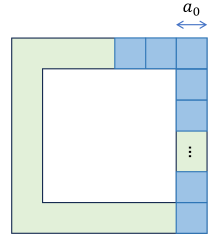
Figure 1: Division of the cube into smoother small regions and the general region.

C.3 Basic bounds of $p_{t}(x)$ and $v_{t}(x)$

Recall that

$$p_{t}({\bm{x}})=\int_{[-1,1]^{d}}\frac{1}{(2\pi\sigma_{t})^{d}}e^{-\frac{\|{\bm{x}}-m_{t}{\bm{y}}\|^{2}}{2\sigma_{t}^{2}}}p_{0}({\bm{y}})d{\bm{y}}.$$

Lemma 16.

There exists $C_{1}=C_{1}(d,C_{0})>0$ such that

$$C_{1}^{-1}\exp\Bigl{(}-\frac{(\|{\bm{x}}\|_{\infty}-m_{t})_{+}^{2}}{\sigma_{t}^{2}}\Bigr{)}\leq p_{t}({\bm{x}})\leq C_{1}\exp\Bigl{(}-\frac{(\|{\bm{x}}\|_{\infty}-m_{t})_{+}^{2}}{2\sigma_{t}^{2}}\Bigr{)}$$ (31)

for any ${\bm{x}}\in{\mathbb{R}}^{d}$ and $t\in[T_{0},1]$.

Proof.

Same as Oko et al. [21, Lemma A.2]. ∎

Lemma 17.

1. Let $k\in{\mathbb{N}}$ be arbitrary. There is $C_{2}=C_{2}(d,k,C_{0})>0$ such that

   $$\left\|\partial_{x_{i_{1}}}\cdots\partial_{x_{i_{k}}}p_{t}({\bm{x}})\right\|\leq\frac{C_{2}}{\sigma_{t}^{k}}\quad(\forall t\in[T_{0},1]).$$

2. There is $C_{3}=C_{3}(d,C_{0})>0$ such that

   $$\|{\bm{v}}_{t}({\bm{x}})\|\leq C_{3}\Bigl{\{}\sigma_{t}^{\prime}\Bigl{(}\frac{(\|{\bm{x}}\|_{\infty}-m_{t})_{+}}{\sigma_{t}}\lor 1\Bigr{)}+|m_{t}^{\prime}|\Bigr{\}}$$

   for any ${\bm{x}}\in{\mathbb{R}}^{d}$ and $t\in[T_{0},1]$.

Proof.

(i) is exactly the same as Lemma A.3, Oko et al 2023.

For (ii), let $g({\bm{x}};m_{t}{\bm{y}},\sigma_{t}^{2})=p_{t}({\bm{x}}|{\bm{y}})=\frac{1}{(2\pi\sigma_{t})^{d/2}}\exp\bigl{\{}-\frac{\|x-m_{t}{\bm{y}}\|^{2}}{2\sigma_{t}^{2}}\bigr{\}}$. Note that

$$v_{t}({\bm{x}})=\frac{\int v_{t}({\bm{x}}|{\bm{y}})g({\bm{x}};m_{t}{\bm{y}},\sigma_{t}^{2})p_{0}({\bm{y}})d{\bm{y}}}{p_{t}({\bm{x}})}.$$

The norm of the numerator is upper bounded by

$$\left\|\int\Bigl{\{}\sigma_{t}^{\prime}\frac{{\bm{x}}-m_{t}{\bm{y}}}{\sigma_{t}}+m_{t}^{\prime}y\Bigr{\}}g({\bm{x}};m_{t}{\bm{y}},\sigma_{t}^{2})p_{0}({\bm{y}})d{\bm{y}}\right\|$$

$$\leq \sigma_{t}^{\prime}\Bigl{\|}\int\frac{{\bm{x}}-m_{t}{\bm{y}}}{\sigma_{t}}g({\bm{x}};m_{t}{\bm{y}},\sigma_{t}^{2})p_{0}({\bm{y}})d{\bm{y}}\Bigr{\|}+|m_{t}^{\prime}|\int\|{\bm{y}}\|g({\bm{x}};m_{t}{\bm{y}},\sigma_{t}^{2})p_{0}({\bm{y}})d{\bm{y}}.$$

Since $\text{Supp}(p_{0})=[-1,1]^{d}$ by assumption (A1), the second term in the last line is upper bounded by

$$|m_{t}^{\prime}|\int g({\bm{x}};m_{t}{\bm{y}},\sigma_{t}^{2})p_{0}({\bm{y}})d{\bm{y}}=|m_{t}^{\prime}|p_{t}({\bm{x}}).$$ (32)

To bound the first term, we use the restriction of the integral region as in Lemma F.9, [21]. Namely, letting $\varepsilon:=C_{1}^{-1}\exp(-\frac{(\|{\bm{x}}\|_{\infty}-m_{t})_{+}^{2})}{2\sigma_{t}^{2}}$, the lower bound of $p_{t}({\bm{x}})$, the integral is approximated as for any $j=1,\ldots,d$,

$$\left|\int_{{\mathbb{R}}^{d}}\Bigl{(}\frac{x_{j}-m_{t}y_{j}}{\sigma_{t}}\Bigr{)}^{\alpha}g({\bm{x}};m_{t}{\bm{y}},\sigma_{t}^{2})p_{0}({\bm{y}})d{\bm{y}}-\int_{A_{x}}\Bigl{(}\frac{x_{j}-m_{t}y_{j}}{\sigma_{t}}\Bigr{)}^{\alpha}g({\bm{x}};m_{t}{\bm{y}},\sigma_{t}^{2})p_{0}({\bm{y}})d{\bm{y}}\right|\leq\varepsilon,$$

where $A_{x}:=\prod_{i=1}^{d}\bigl{[}\frac{x_{i}}{m_{t}}-\frac{C\sigma_{c}}{m_{t}}\sqrt{\log(1/\varepsilon)},\frac{x_{i}}{m_{t}}+\frac{C\sigma_{t}}{m_{t}}\sqrt{\log(1/\varepsilon)}\bigr{]}$, $C$ is a positive constant depending only on $d$, and $\alpha\in\{0,1\}$. Then, the first term is upper-bounded by

$$\sigma_{t}^{\prime}\Bigl{\|}\int_{A_{x}}\frac{x-m_{t}{\bm{y}}}{\sigma_{t}}g({\bm{x}};m_{t}{\bm{y}},\sigma_{t}^{2})p_{0}({\bm{y}})d{\bm{y}}+\varepsilon{\bf 1}\Bigr{\|}.$$

Noting that ${\bm{y}}\in A_{x}$ is equivalent to $|x_{i}-m_{t}y_{i}|/\sigma_{t}\leq C\sqrt{\log(1/\varepsilon)}$, the above quantity is further upper-bounded by

$$\sqrt{d}C\sigma_{t}^{\prime}\sqrt{\log(1/\varepsilon)}\int_{A_{x}}g({\bm{x}};m_{t}{\bm{y}},\sigma_{t}^{2})p_{0}({\bm{y}})d{\bm{y}}+\sqrt{d}\varepsilon\leq C^{\prime}\Bigl{(}\sigma_{t}^{\prime}\sqrt{\log(1/\varepsilon)}p_{t}({\bm{x}})+\varepsilon\Bigr{)}.$$

Noting that $\varepsilon=C_{1}^{-1}\exp(-\frac{(\|{\bm{x}}\|_{\infty}-m_{t})_{+}^{2})}{\sigma_{t}^{2}})$ and $p_{t}({\bm{x}})\geq\varepsilon$, we obtain

$$\|v_{t}({\bm{x}})\| \leq\frac{C^{\prime}(\sigma_{t}^{\prime}\sqrt{\log(1/\varepsilon)}p_{t}({\bm{x}})+\varepsilon)+|m_{t}^{\prime}|p_{t}({\bm{x}})}{p_{t}({\bm{x}})}$$

$$\leq C^{\prime\prime}\left\{\sigma_{t}^{\prime}\Bigl{(}\frac{(\|{\bm{x}}\|_{\infty}-m_{t})_{+}}{\sigma_{t}}\Bigr{)}+\sigma_{t}^{\prime}+|m_{t}^{\prime}|\right\}$$

$$\leq C^{\prime\prime\prime}\left\{\sigma_{t}^{\prime}\Bigl{(}\frac{(\|{\bm{x}}\|_{\infty}-m_{t})_{+}}{\sigma_{t}}\vee 1\Bigr{)}+|m_{t}^{\prime}|\right\}.$$

This completes the proof. ∎

The following lemma shows an upper bound of ${\bm{v}}_{t}({\bm{x}})$ when ${\bm{x}}$ is in a bounded region of $\sigma_{t}\sqrt{1/\varepsilon}$, and presents bounds of relevant integrals.

Lemma 18.

Let $\varepsilon>0$ is sufficiently small.

1. For any $C_{4}>0$, we have

   $$\|{\bm{v}}_{t}({\bm{x}})\|\leq C_{4}\bigl{(}\sigma_{t}^{\prime}\sqrt{\log(1/\varepsilon)}+|m_{t}^{\prime}|\bigr{)}$$ (33)

   for any ${\bm{x}}$ with $\|{\bm{x}}\|_{\infty}\leq m_{t}+C_{4}\sigma_{t}\sqrt{\log(1/\varepsilon)}$ and $t\in[T_{0},1]$.

2. For any $C_{5}>0$, there is $\tilde{C}>0$ such that

   $$\int_{\|{\bm{x}}\|_{\infty}\geq m_{t}+C_{5}\sigma_{t}\sqrt{\log(1/\varepsilon)}}p_{t}({\bm{x}})\|v_{t}({\bm{x}})\|^{2}d{\bm{x}}\leq\tilde{C}\bigl{\{}(\sigma_{t}^{\prime})^{2}\log^{\frac{d}{2}}\bigl{(}\varepsilon^{-1}\bigr{)}+(m_{t}^{\prime})^{2}\log^{\frac{d-2}{2}}\bigl{(}\varepsilon^{-1}\bigr{)}\bigr{\}}\varepsilon^{\frac{C_{5}^{2}}{2}}$$ (34)

   and

   $$\int_{\|{\bm{x}}\|_{\infty}\geq m_{t}+C_{5}\sigma_{t}\sqrt{\log(1/\varepsilon)}}p_{t}({\bm{x}})d{\bm{x}}|\leq\tilde{C}\log^{\frac{d-2}{2}}\bigl{(}\varepsilon^{-1}\bigr{)}\varepsilon^{\frac{C_{5}^{2}}{2}}$$ (35)

   hold for any $\varepsilon>0$ and $t\in[T_{0},1]$.

Proof.

(i) is obvious from Lemma 17, since $(|{\bm{x}}\|_{\infty}-m_{t})_{+}/\sigma_{t}\leq C_{4}\sqrt{\log(1/\varepsilon)}$ under the assumption of ${\bm{x}}$.

We show (ii). It follows from Lemmas 16 and 17 that

$$p_{t}({\bm{x}})\|{\bm{v}}_{t}({\bm{x}})\|^{2}\leq 2C_{1}C_{3}\exp\Bigl{(}-\frac{(\|{\bm{x}}\|_{\infty}-m_{t}{\bm{y}})_{+}^{2}}{2\sigma_{t}^{2}}\Bigr{)}\Bigl{\{}(\sigma_{t}^{\prime})^{2}\frac{(\|{\bm{x}}\|_{\infty}-m_{t})_{+}^{2}}{\sigma_{t}^{2}}+(m_{t}^{\prime})^{2}\Bigr{\}}.$$

Let $r:=(\|{\bm{x}}\|_{\infty}-m_{t})_{+}/\sigma_{t}$ and $B_{i}:=\{{\bm{x}}=(x_{1},\ldots,x_{d})\in{\mathbb{R}}^{d}\mid|x_{i}|=\max_{1\leq j\leq d}|x_{j}|$. The space is divided into $d$ regions $\cup_{i=1}^{d}B_{i}$ with measure-zero intersections. In $B_{1}$, the variables $x_{2},\ldots,x_{d}$ satisfy $|x_{j}|\leq m_{t}+C_{4}\sigma_{t}\sqrt{\log(1/\varepsilon)}$, and integral (34) is upper bounded by

$$2C_{1}C_{3}d\int_{C_{4}\sqrt{\log(1/\varepsilon)}}e^{-\frac{r^{2}}{2}}\bigl{(}(\sigma_{t}^{\prime})^{2}r^{2}+(m_{t}^{\prime})^{2}\bigr{\}}(\sigma_{t}r+m_{t})^{d-1}dr$$

$$\leq C^{\prime}\int_{C_{4}\sqrt{\log(1/\varepsilon)}}e^{-\frac{r^{2}}{2}}\bigl{(}(\sigma_{t}^{\prime})^{2}r^{d+1}+(m_{t}^{\prime})^{2}r^{d-1}\bigr{\}}dr,$$

where we use $(\sigma_{t}r+m_{t})^{d-1}\leq(r+1)^{d-1}\leq 2^{d-1}r^{d-1}$.

For $\ell\in{\mathbb{N}}\cup\{0\}$, define

$$\psi_{\ell}(z):=\int_{z}^{\infty}r^{\ell}e^{-\frac{r^{2}}{2}}dr.$$

It is easy to see $\psi_{1}(z)=e^{-\frac{z^{2}}{2}}$ and $\psi_{\ell}(z)=x^{\ell-1}e^{-\frac{z^{2}}{2}}+(\ell-1)\psi_{\ell-1}(z)$ by partial integral. Using these formula, we can see that for $z\geq 1$

$$\psi_{\ell}(z)\leq B_{\ell}z^{\ell-1}e^{-\frac{z^{2}}{2}},$$

where $B_{\ell}$ is a positive constant that depends only on $\ell$.

Thus we obtain an upper bound

$$\tilde{C}\bigl{\{}(\sigma_{t}^{\prime})^{2}\log^{\frac{d}{2}}\bigl{(}\frac{1}{\varepsilon}\bigr{)}+(m_{t}^{\prime})^{2}\log^{\frac{d-2}{2}}\bigl{(}\frac{1}{\varepsilon}\bigr{)}\bigr{\}}\varepsilon^{\frac{C_{5}^{2}}{2}},$$

which proves (34). The assertion (35) is similar. ∎

C.4 Bounds of the approximation error for small $t$

This subsection shows the proof of Theorem 6.

(I) Restriction of the integral.

We first show that the left hand side of (17) can be approximated by the integral over the bounded region

$$D_{t,N}:=\{{\bm{x}}\in{\mathbb{R}}^{d}\mid\|{\bm{x}}\|_{\infty}\leq m_{t}+C_{4}\sigma_{t}\sqrt{\log N}\}.$$

To see this, observe that from Lemma 17 (ii), for ${\bm{x}}\in D_{t,N}$ we have

$$\|{\bm{v}}_{t}({\bm{x}})\|^{2}\leq 2C_{3}^{2}\left\{(\sigma_{t}^{\prime})^{2}\log N+|m_{t}^{\prime}|^{2}\right\}.$$ (36)

From the bound of ${\bm{v}}_{t}({\bm{x}})$, we can restrict the neural network $\bm{\phi}({\bm{x}},t)$ so that it satisfies the same upper bound. Therefore, (36) is applied to $\|\bm{\phi}({\bm{x}},t)\|^{2}$ also. Combining this fact with Lemma 18 (ii), we have

$$\int_{D_{t,N}^{C}}\|\bm{\phi}({\bm{x}},t)-{\bm{v}}_{t}({\bm{x}})\|^{2}p_{t}({\bm{x}})d{\bm{x}}$$

$$\leq 4C_{3}^{2}\left\{(\sigma_{t}^{\prime})^{2}\log N+|m_{t}^{\prime}|^{2}\right\}\int_{D_{t,N}^{C}}\frac{1}{(\sqrt{2\pi}\sigma)^{d}}e^{-\frac{\|{\bm{x}}-m_{t}{\bm{y}}\|^{2}}{2\sigma^{2}}}d{\bm{x}}$$

$$\leq 4C_{3}^{2}\tilde{C}\left\{(\sigma_{t}^{\prime})^{2}\log N+|m_{t}^{\prime}|^{2}\right\}N^{-C_{4}^{2}/2}\log^{\frac{d-2}{2}}N.$$

If $C_{4}$ is taken large enough to satisfy $C_{4}^{2}/2>\frac{2s}{d}$, it follows that

$$\int\|\bm{\phi}({\bm{x}},t)-{\bm{v}}_{t}({\bm{x}})\|^{2}p_{t}({\bm{x}})d{\bm{x}}\\ \leq\int_{D_{t,N}}\|\bm{\phi}({\bm{x}},t)-{\bm{v}}_{t}({\bm{x}})\|^{2}p_{t}({\bm{x}})d{\bm{x}}+C^{\prime}\left\{(\sigma_{t}^{\prime})^{2}\log N+|m_{t}^{\prime}|^{2}\right\}N^{-\frac{2s}{d}}$$ (37)

for some constant $C^{\prime}>0$. Thus, we can consider the first term on the right-hand side.

Let $\omega>0$ be an arbitrary positive number. The integral over $D_{t,N}$ in (37) can be restricted to the region $\{{\bm{x}}\mid p_{t}({\bm{x}})\geq N^{-\frac{2s+\omega}{d}}\}$. This can be easily seen by

$$\int_{D_{t,N}}{\bf 1}[p_{t}({\bm{x}})\leq N^{-\frac{2s+\omega}{d}}]\|{\bm{v}}_{t}({\bm{x}})-\bm{\phi}({\bm{x}},t)\|^{2}p_{t}({\bm{x}})d{\bm{x}}$$

$$\leq 4C_{3}^{2}\int_{D_{t,N}}\left\{(\sigma_{t}^{\prime})^{2}\log N+|m_{t}^{\prime}|^{2}\right\}N^{-\frac{2s+\omega}{d}}d{\bm{x}}$$

$$\leq 4C_{3}^{2}N^{-\frac{2s+\omega}{d}}\left\{(\sigma_{t}^{\prime})^{2}\log N+|m_{t}^{\prime}|^{2}\right\}2^{d}(m_{t}+C_{4}\sigma_{t}\sqrt{\log N})^{d}$$

$$\leq C^{\prime\prime}\left\{(\sigma_{t}^{\prime})^{2}\log N+|m_{t}^{\prime}|^{2}\right\}N^{-\frac{2s+\omega}{d}}\log^{\frac{d}{2}}N,$$

where $C^{\prime\prime}$ depends only on $d$, $C_{3}$, and $C_{4}$. This bound is of smaller order than the second term of the right hand side of (37), and thus negligible. In sumamry, we have

$$\int\|\bm{\phi}({\bm{x}},t)-{\bm{v}}_{t}({\bm{x}})\|^{2}p_{t}({\bm{x}})d{\bm{x}}\\ \leq\int_{D_{t,N}}{\bf 1}[p_{t}({\bm{x}})\geq N^{-\frac{2s+\omega}{d}}]\|\bm{\phi}({\bm{x}},t)-{\bm{v}}_{t}({\bm{x}})\|^{2}p_{t}({\bm{x}})d{\bm{x}}+C^{\prime}\left\{(\sigma_{t}^{\prime})^{2}\log N+|m_{t}^{\prime}|^{2}\right\}N^{-\frac{2s}{d}}$$ (38)

for sufficiently large $N$.

(II) Decomposition of integral. Here we give a bound of the integral $\int\|\bm{\phi}({\bm{x}},t)-{\bm{v}}_{t}({\bm{x}})\|^{2}p_{t}({\bm{x}})d{\bm{x}}$ over the region $D_{t,N}\cap\{{\bm{x}}\mid p_{t}({\bm{x}})\geq N^{-\frac{2s+\omega}{d}}\}$. The norm $\|\bm{\phi}({\bm{x}},t)-{\bm{v}}_{t}({\bm{x}})\|$ is bounded in detail.

First, recall that

$${\bm{v}}_{t}({\bm{x}})=\frac{\int{\bm{v}}_{t}({\bm{x}}|{\bm{y}})p_{t}({\bm{x}}|{\bm{y}})p_{0}({\bm{y}})d{\bm{y}}}{p_{t}({\bm{x}})},\quad p_{t}({\bm{x}})=\int p_{t}({\bm{x}}|{\bm{y}})p_{0}({\bm{y}})d{\bm{y}}.$$ (39)

Based on Theorem 13, we can find $f_{N}$ in (24) such that

$$\|p_{0}-f_{N}\|_{L^{2}(I^{d})}\leq C_{a}N^{-s/d},\qquad\|p_{0}-f_{N}\|_{L^{2}(I^{d}\backslash I_{N}^{d})}\leq C_{a}N^{-\check{s}/d}$$ (40)

As an approximate of $p_{t}({\bm{x}})$, define a function $\tilde{f}_{1}({\bm{x}},t)$ by

$$\tilde{f}_{1}({\bm{x}},t):=\int\frac{1}{(\sqrt{2\pi}\sigma_{t})^{d}}e^{-\frac{\|{\bm{x}}-m_{t}{\bm{y}}\|^{2}}{2\sigma_{t}^{2}}}f_{N}({\bm{y}})d{\bm{y}}.$$ (41)

Since we consider the region where $p_{t}({\bm{x}})\geq N^{-(2s+\omega)/d}$, we further define

$$f_{1}({\bm{x}},t):=\tilde{f}_{1}({\bm{x}},t)\vee N^{-\frac{2s+\omega}{d}}.$$

In a similar manner, the numerator of (39) can be approximated by

$$\sigma_{t}^{\prime}{\bm{f}}_{2}({\bm{x}},t)+m_{t}^{\prime}{\bm{f}}_{3}({\bm{x}},t),$$

where ${\mathbb{R}}^{d}$-valued functions ${\bm{f}}_{2}$ and ${\bm{f}}_{3}$ are defined by

$${\bm{f}}_{2}({\bm{x}},t) :=\int\frac{{\bm{x}}-m_{t}{\bm{y}}}{\sigma_{t}}\frac{1}{(\sqrt{2\pi}\sigma_{t})^{d}}e^{-\frac{\|{\bm{x}}-m_{t}{\bm{y}}\|^{2}}{2\sigma_{t}^{2}}}f_{N}({\bm{y}})d{\bm{y}}.$$

$${\bm{f}}_{3}({\bm{x}},t) :=\int{\bm{y}}\frac{1}{(\sqrt{2\pi}\sigma_{t})^{d}}e^{-\frac{\|{\bm{x}}-m_{t}{\bm{y}}\|^{2}}{2\sigma_{t}^{2}}}f_{N}({\bm{y}})d{\bm{y}}.$$ (42)

We have an approximate of ${\bm{v}}_{t}({\bm{x}})$ by

$${\bm{f}}_{4}({\bm{x}},t):=\frac{\sigma_{t}^{\prime}{\bm{f}}_{2}({\bm{x}},t)+m_{t}^{\prime}{\bm{f}}_{3}({\bm{x}},t)}{f_{1}({\bm{x}},t)}{\bf 1}\left[\left|\frac{{\bm{f}}_{2}}{f_{1}}\right|\leq C_{5}\sqrt{\log N}\right]{\bf 1}\left[\left|\frac{{\bm{f}}_{3}}{f_{1}}\right|\leq C_{5}\right].$$

We want to evaluate

$$\int_{D_{t,N}}{\bf 1}[p_{t}({\bm{x}})\geq N^{-\frac{2s+\omega}{d}}]\|\bm{\phi}({\bm{x}},t)-{\bm{v}}_{t}({\bm{x}})\|^{2}p_{t}({\bm{x}})d{\bm{x}}$$

$$\leq\int_{D_{t,N}}{\bf 1}[p_{t}({\bm{x}})\geq N^{-\frac{2s+\omega}{d}}]\|\bm{\phi}({\bm{x}},t)-{\bm{f}}_{4}({\bm{x}},t)\|^{2}p_{t}({\bm{x}})d{\bm{x}}$$

$$\qquad+\int_{D_{t,N}}{\bf 1}[p_{t}({\bm{x}})\geq N^{-\frac{2s+\omega}{d}}]\|{\bm{f}}_{4}({\bm{x}},t)-{\bm{v}}_{t}({\bm{x}})\|^{2}p_{t}({\bm{x}})d{\bm{x}}$$

$$=:I_{A}+I_{B}.$$ (43)

(III) Bound of $I_{A}$ (neural network approximation of B-spline)

We will approximate $f_{1}$, ${\bm{f}}_{2}$, and ${\bm{f}}_{3}$ by nerual networks. For $k\in{\mathbb{Z}}_{+}$ and $j\in{\mathbb{Z}}^{d}$, let $E^{(a)}_{k,j,u}$ ($a=1,2,3$, $u=0,1$) denote the functions defined by

$$E^{(1)}_{k,j,u}:=\int_{{\mathbb{R}}^{d}}{\bf 1}\left[\|{\bm{y}}\|_{\infty}\leq C_{b,1}\right]M^{d}_{k,j}({\bm{y}})\frac{1}{(\sqrt{2\pi}\sigma_{t})^{d}}e^{-\frac{\|{\bm{x}}-m_{t}{\bm{y}}\|^{2}}{2\sigma_{t}^{2}}}d{\bm{y}},$$ (44)

$$E^{(2)}_{k,j,u}:=\int_{{\mathbb{R}}^{d}}\frac{{\bm{x}}-m_{t}{\bm{y}}}{\sigma_{t}}{\bf 1}\left[\|{\bm{y}}\|_{\infty}\leq C_{b,1}\right]M^{d}_{k,j}({\bm{y}})\frac{1}{(\sqrt{2\pi}\sigma_{t})^{d}}e^{-\frac{\|{\bm{x}}-m_{t}{\bm{y}}\|^{2}}{2\sigma_{t}^{2}}}d{\bm{y}},$$ (45)

and

$$E^{(3)}_{k,j,u}:=\int_{{\mathbb{R}}^{d}}{\bm{y}}{\bf 1}\left[\|{\bm{y}}\|_{\infty}\leq C_{b,1}\right]M^{d}_{k,j}({\bm{y}})\frac{1}{(\sqrt{2\pi}\sigma_{t})^{d}}e^{-\frac{\|{\bm{x}}-m_{t}{\bm{y}}\|^{2}}{2\sigma_{t}^{2}}}d{\bm{y}},$$ (46)

where $C_{b,1}=1$ for $u=0$ and $C_{b,1}=1-N^{-\frac{\kappa^{-1}-\delta}{d}}$ for $u=1$. Then, from Theorem 12, $f_{N}$ is written as a linear combination of ${\bf 1}[\|{\bm{y}}\|_{\infty}\leq C_{b,1}]M^{d}_{k,j}$ with coefficients $\alpha_{k,j}$. From Theorem 13, for any $\varepsilon>0$, there are neural networks $\phi_{5},\bm{\phi}_{6}$ and $\bm{\phi}_{7}$ such that

$$|f_{1}({\bm{x}},t)-\phi_{5}({\bm{x}},t)| \leq D_{5}N\max_{i}|\alpha_{i}|\varepsilon$$

$$\|{\bm{f}}_{2}({\bm{x}},t)-\bm{\phi}_{6}({\bm{x}},t)\| \leq D_{6}N\max_{i}|\alpha_{i}|\varepsilon,$$

$$\|{\bm{f}}_{3}({\bm{x}},t)-\bm{\phi}_{7}({\bm{x}},t)\| \leq D_{7}N\max_{i}|\alpha_{i}|\varepsilon.$$

Since $\max_{i}|\alpha_{i}|\leq N^{-(\nu^{-1}+d^{-1})(d/p-s)_{+}}$, by taking $\varepsilon$ sufficently small, for any $\eta>0$ we have

$$|f_{1}({\bm{x}},t)-\phi_{5}({\bm{x}},t)| \leq D_{5}N^{-\eta}$$

$$\|{\bm{f}}_{2}({\bm{x}},t)-\bm{\phi}_{6}({\bm{x}},t)\| \leq D_{6}N^{-\eta}$$

$$\|{\bm{f}}_{3}({\bm{x}},t)-\bm{\phi}_{7}({\bm{x}},t)\| \leq D_{7}N^{-\eta}.$$

The operations to obtain the approximation of ${\bm{v}}_{t}({\bm{x}})$ based on $\phi_{5}$, $\bm{\phi}_{6}$, and $\bm{\phi}_{7}$ are given by the following procedures:

$$\zeta_{1} :=\texttt{clip}(\phi_{5};N^{-(2s+\omega)/d},N^{K_{0}+1}),$$

$$\zeta_{2} :=\texttt{recip}(\zeta_{1}),$$

$${\bm{\zeta}}_{3} :=\texttt{mult}(\zeta_{2},\bm{\phi}_{6}),$$

$${\bm{\zeta}}_{4} :=\texttt{clip}({\bm{\zeta}}_{3};-C_{5}\sqrt{\log N},C_{5}\sqrt{\log N}),$$

$${\bm{\zeta}}_{5} :=\texttt{mult}(\zeta_{2},\bm{\phi}_{7}),$$

$${\bm{\zeta}}_{6} :=\texttt{clip}({\bm{\zeta}}_{5};-C_{5},C_{5}),$$

$${\bm{\zeta}}_{7} :=\texttt{mult}({\bm{\zeta}}_{4},\hat{\sigma^{\prime}}),$$

$${\bm{\zeta}}_{8} :=\texttt{mult}({\bm{\zeta}}_{6},\hat{m^{\prime}}),$$

$$\bm{\phi}_{8} :={\bm{\zeta}}_{7}+{\bm{\zeta}}_{8}.$$

As shown in Section D, the neural networks clip, recip, and mult achieve the approximation error $N^{-\eta}$ with arbitrarily large $\eta$, while the complexity of the networks increases only at most polynomials of $N$ for $B$ and $\|W\|_{\infty}$, and at most ${\rm poly}(\log N)$ factor for $L$ and $S$. In the upper bound of the generalization error, the network parameters $B$ and $\|W\|_{\infty}$ and the inverse error $\varepsilon^{-1}=N^{\eta}$ appear only in the $\log()$ part to the log covering number, and $S$ and $B$ appear as a linear factor. We also need to use approximation $\hat{\sigma_{t}^{\prime}}$ and $\hat{m_{t}^{\prime}}$ of $\sigma_{t}^{\prime}$ and $m_{t}^{\prime}$, respectively, by neural networks in construction. However, this can be done in a similar manner to [Section B1, 21] with all the network parameters $O(\log^{r}\varepsilon^{-1})$ for approximation accuracy $\varepsilon$, and thus they have only $O({\rm poly}(\log N))$ contributions. We omit the details in this paper. Consequently, the increase of the neural networks to obtain $\bm{\phi}_{8}$ from $\phi_{5}$, $\bm{\phi}_{6}$, and $\bm{\phi}_{7}$ contributes the log covering number only by the ${\rm poly}(\log N)$ factor.

As a result, we obtain

$$I_{A}=O(N^{-\eta}{\rm poly}(\log N))$$ (47)

for arbitrary $\eta>0$, while the required neural network increases the complexity term only by $O({\rm poly}(\log N))$ factor.

(IV) Bound of $I_{B}$ (B-spline approximation of the true vector field)

We evaluate here

$$I_{B}=\int_{D_{t,N}}{\bf 1}[p_{t}({\bm{x}})\geq N^{-\frac{2s+\omega}{d}}]\|{\bm{f}}_{4}({\bm{x}},t)-{\bm{v}}_{t}({\bm{x}})\|^{2}p_{t}({\bm{x}})d{\bm{x}}.$$ (48)

Let ${\bm{h}}_{2}({\bm{x}},t)$ and ${\bm{h}}_{3}({\bm{x}},t)$ be functions defined by

$${\bm{h}}_{2}({\bm{x}},t) :=\int_{{\mathbb{R}}^{d}}\frac{{\bm{x}}-m_{t}{\bm{y}}}{\sigma_{t}}\frac{1}{(\sqrt{2\pi}\sigma_{t})^{d}}e^{-\frac{\|{\bm{x}}-m_{t}{\bm{y}}\|^{2}}{2\sigma_{t}^{2}}}p_{0}({\bm{y}})d{\bm{y}},$$

$${\bm{h}}_{3}({\bm{x}},t) :=\int_{{\mathbb{R}}^{d}}{\bm{y}}\frac{1}{(\sqrt{2\pi}\sigma_{t})^{d}}e^{-\frac{\|{\bm{x}}-m_{t}{\bm{y}}\|^{2}}{2\sigma_{t}^{2}}}p_{0}({\bm{y}})d{\bm{y}}.$$ (49)

Then,

$$\|{\bm{f}}_{4}({\bm{x}},t)-{\bm{v}}_{t}({\bm{x}})\|$$

$$={\bf 1}\left[\left\|\frac{{\bm{f}}_{2}}{f_{1}}\right\|\leq C_{5}\sqrt{\log N}\right]{\bf 1}\left[\left\|\frac{{\bm{f}}_{3}}{f_{1}}\right\|\leq C_{5}\right]\left\|\frac{\sigma_{t}^{\prime}{\bm{f}}_{2}({\bm{x}},t)+m_{t}^{\prime}{\bm{f}}_{3}({\bm{x}},t)}{f_{1}({\bm{x}})}-\frac{\sigma_{t}^{\prime}{\bm{h}}_{2}({\bm{x}},t)+m_{t}^{\prime}{\bm{h}}_{3}({\bm{x}},t)}{p_{t}({\bm{x}})}\right\|.$$ (50)

We evaluate the integral (48) by dividing $D_{t,N}$ into the two domains $\{{\bm{x}}\mid\|{\bm{x}}\|_{\infty}\leq m_{t}\}$ and $\{{\bm{x}}\mid m_{t}\leq\|{\bm{x}}\|_{\infty}\leq m_{t}+C_{4}\sigma_{t}\sqrt{\log N}\}$.

Because of the condition $p_{t}({\bm{x}})\geq N^{-(2s+\omega)/d}$, it suffices to take the network $f_{1}({\bm{x}},t)$ so that it satisfies $f_{1}({\bm{x}},t)\geq N^{-(2s+\omega)/d}$ by clipping the function if necessary. We therefore assume in the sequel that $f_{1}({\bm{x}},t)\geq N^{-(2s+\omega)/d}$ holds.

(IV-a) case: $\|{\bm{x}}\|_{\infty}\leq m_{t}$.

In this case, Lemma 16 shows that $C_{1}^{-1}\leq p_{t}(x)\leq C_{1}$ for some $C_{1}>0$, which depends only on $d$ and $p_{0}$. Using this fact and the conditions $\bigl{\|}\frac{{\bm{f}}_{2}}{f_{1}}\bigr{\|}\leq C_{5}\sqrt{\log N}$ and $\bigl{\|}\frac{{\bm{f}}_{3}}{f_{1}}\bigr{\|}\leq C_{5}$, we have

$$\left\|\frac{\sigma_{t}^{\prime}{\bm{f}}_{2}({\bm{x}},t)+m_{t}^{\prime}{\bm{f}}_{3}({\bm{x}},t)}{f_{1}({\bm{x}})}-\frac{\sigma_{t}^{\prime}{\bm{h}}_{2}({\bm{x}},t)+m_{t}^{\prime}{\bm{h}}_{3}({\bm{x}},t)}{p_{t}({\bm{x}})}\right\|$$

$$\leq|\sigma_{t}^{\prime}|\left\|\frac{{\bm{f}}_{2}({\bm{x}},t)}{f_{1}({\bm{x}})}-\frac{{\bm{h}}_{2}({\bm{x}},t)}{p_{t}({\bm{x}})}\right\|+|m_{t}^{\prime}|\left\|\frac{{\bm{f}}_{3}({\bm{x}},t)}{f_{1}({\bm{x}})}-\frac{{\bm{h}}_{3}({\bm{x}},t)}{p_{t}({\bm{x}})}\right\|$$

$$\leq|\sigma_{t}^{\prime}|\left\{\left\|\frac{{\bm{f}}_{2}(x)}{f_{1}({\bm{x}})}-\frac{{\bm{f}}_{2}({\bm{x}},t)}{p_{t}({\bm{x}})}\right\|+\left\|\frac{{\bm{f}}_{2}({\bm{x}},t)}{p_{t}({\bm{x}})}-\frac{{\bm{h}}_{2}({\bm{x}},t)}{p_{t}({\bm{x}})}\right\|\right\}$$

$$\qquad\qquad+|m_{t}^{\prime}|\left\{\left\|\frac{{\bm{f}}_{3}(x)}{f_{1}({\bm{x}})}-\frac{{\bm{f}}_{3}({\bm{x}},t)}{p_{t}({\bm{x}})}\right\|+\left\|\frac{{\bm{f}}_{3}({\bm{x}},t)}{p_{t}({\bm{x}})}-\frac{{\bm{h}}_{3}({\bm{x}},t)}{p_{t}({\bm{x}})}\right\|\right\}$$

$$\leq C_{1}|\sigma_{t}^{\prime}|\left\{C_{5}\sqrt{\log N}|p_{t}({\bm{x}})-f_{1}({\bm{x}},t)|+\|{\bm{f}}_{2}({\bm{x}},t)-{\bm{h}}_{2}({\bm{x}},t)\|\right\}$$

$$\qquad\qquad+C_{1}|m_{t}^{\prime}|\left\{C_{5}|p_{t}({\bm{x}})-f_{1}({\bm{x}},t)|+\|{\bm{f}}_{3}({\bm{x}},t)-{\bm{h}}_{3}({\bm{x}},t)\|\right\}$$

$$\leq\tilde{C}\left\{(|\sigma_{t}^{\prime}|\sqrt{\log N}+|m_{t}^{\prime}|)|f_{1}({\bm{x}},t)-p_{t}({\bm{x}})|+|\sigma_{t}^{\prime}|\|{\bm{f}}_{2}({\bm{x}},t)-{\bm{h}}_{2}({\bm{x}},t)\|+|m_{t}^{\prime}|\|{\bm{f}}_{3}({\bm{x}},t)-{\bm{h}}_{3}({\bm{x}},t)\|\right\}.$$ (51)

We evaluate the integral on $\{{\bm{x}}\mid\|{\bm{x}}\|_{\infty}\leq m_{t}\}$. From the bound (51), we have

$$I_{B,1} :=\int_{\|{\bm{x}}\|_{\infty}\leq m_{t}}{\bf 1}[p_{t}({\bm{x}})\geq N^{-\frac{2s+\omega}{d}}]\|{\bm{f}}_{4}({\bm{x}},t)-{\bm{v}}_{t}({\bm{x}})\|^{2}p_{t}({\bm{x}})d{\bm{x}}$$

$$\leq C^{\prime}\left[\left\{(\sigma_{t}^{\prime})^{2}\log N+(m_{t}^{\prime})^{2}\right\}\int_{\|{\bm{x}}\|_{\infty}\leq m_{t}}{\bf 1}[p_{t}({\bm{x}})\geq N^{-\frac{2s+\omega}{d}}]|f_{1}({\bm{x}},t)-p_{t}({\bm{x}})|^{2}p_{t}({\bm{x}})d{\bm{x}}\right.$$

$$\qquad\qquad+(\sigma_{t}^{\prime})^{2}\int_{\|{\bm{x}}\|_{\infty}\leq m_{t}}{\bf 1}[p_{t}({\bm{x}})\geq N^{-\frac{2s+\omega}{d}}]\|{\bm{f}}_{2}({\bm{x}},t)-{\bm{h}}_{2}({\bm{x}},t)\|^{2}p_{t}({\bm{x}})d{\bm{x}}$$

$$\qquad\qquad\left.+(m_{t}^{\prime})^{2}\int_{\|{\bm{x}}\|_{\infty}\leq m_{t}}{\bf 1}[p_{t}({\bm{x}})\geq N^{-\frac{2s+\omega}{d}}]\|{\bm{f}}_{3}({\bm{x}},t)-{\bm{h}}_{3}({\bm{x}},t)\|^{2}p_{t}({\bm{x}})d{\bm{x}}\right].$$ (52)

We write $J_{B}^{(1)}$, $J_{B}^{(2)}$, and $J_{B}^{(3)}$ for the three integrals that appear in the right-hand side of (52).

We will show only the derivation of an upper bound for $J_{B}^{(2)}$, since the other two cases are similar. Recall that by the definition of ${\bm{f}}_{2}$ and ${\bm{h}}_{2}$,

$${\bm{f}}_{2}({\bm{x}},t)-{\bm{h}}_{2}({\bm{x}},t)=\int_{I^{d}}\frac{{\bm{x}}-m_{t}{\bm{y}}}{\sigma_{t}}\frac{1}{(\sqrt{2\pi}\sigma_{t})^{d}}e^{-\frac{\|{\bm{x}}-m_{t}{\bm{y}}\|^{2}}{2\sigma_{t}^{2}}}(f_{N}({\bm{y}})-p_{0}({\bm{y}}))d{\bm{y}}.$$

Then, using $p_{t}(x)\leq C_{1}$, we have

$$J_{B}^{(2)} \leq C_{1}\int_{\|{\bm{x}}\|_{\infty}\leq m_{t}}{\bf 1}[p_{t}({\bm{x}})\geq N^{-\frac{2s+\omega}{d}}]\left\|\int_{I^{d}}\frac{{\bm{x}}-m_{t}{\bm{y}}}{\sigma_{t}}\frac{1}{(\sqrt{2\pi}\sigma_{t})^{d}}e^{-\frac{\|{\bm{x}}-m_{t}{\bm{y}}\|^{2}}{2\sigma_{t}^{2}}}(f_{N}({\bm{y}})-p_{0}({\bm{y}}))d{\bm{y}}\right\|^{2}d{\bm{x}}$$

$$\leq C_{1}\int_{\|{\bm{x}}\|_{\infty}\leq m_{t}}\left\|\frac{1}{m_{t}^{d}}\int_{{\mathbb{R}}^{d}}{\bf 1}[\|{\bm{y}}\|_{\infty}\leq 1]\frac{{\bm{x}}-m_{t}{\bm{y}}}{\sigma_{t}}\left(\frac{m_{t}}{\sqrt{2\pi}\sigma_{t}}\right)^{d}e^{-\frac{\|{\bm{y}}-{\bm{x}}/m_{t}\|^{2}}{2(\sigma_{t}/m_{t})^{2}}}(f_{N}({\bm{y}})-p_{0}({\bm{y}}))d{\bm{y}}\right\|^{2}d{\bm{x}}$$

$$\leq\frac{C_{1}}{m_{t}^{2d}}\int_{\|{\bm{x}}\|_{\infty}\leq m_{t}}\int_{{\mathbb{R}}^{d}}{\bf 1}[\|{\bm{y}}\|_{\infty}\leq 1]\left\|\frac{{\bm{x}}-m_{t}{\bm{y}}}{\sigma_{t}}\right\|^{2}\left(\frac{m_{t}}{\sqrt{2\pi}\sigma_{t}}\right)^{d}e^{-\frac{\|{\bm{y}}-{\bm{x}}/m_{t}\|^{2}}{2(\sigma_{t}/m_{t})^{2}}}(f_{N}({\bm{y}})-p_{0}({\bm{y}}))^{2}d{\bm{y}}d{\bm{x}}$$

$$=\frac{C_{1}}{m_{t}^{d}}\int_{\|{\bm{x}}\|_{\infty}\leq m_{t}}\int_{{\mathbb{R}}^{d}}{\bf 1}[\|{\bm{y}}\|_{\infty}\leq 1]\left\|\frac{{\bm{x}}-m_{t}{\bm{y}}}{\sigma_{t}}\right\|^{2}\frac{1}{(\sqrt{2\pi}\sigma_{t})^{d}}e^{-\frac{\|{\bm{x}}-m_{t}{\bm{y}}\|^{2}}{2\sigma_{t}^{2}}}(f_{N}({\bm{y}})-p_{0}({\bm{y}}))^{2}d{\bm{y}}d{\bm{x}},$$ (53)

where the third line uses Jensen’s inequality for $\|\cdot\|^{2}$. For $t\in 3N^{-\frac{\kappa^{-1}-\delta}{d}}$ with sufficiently large $N$, we can find $c_{0}>0$ such that $m_{t}\geq c_{0}$ on the time interval $[T_{0},3N^{-\frac{\kappa^{-1}-\delta}{d}}]$. We can thus further obtain for some $C^{\prime}>0$

$$J_{B}^{(2)} \leq C^{\prime}\int_{I^{d}}\int_{{\mathbb{R}}^{d}}\frac{\|{\bm{x}}-m_{t}{\bm{y}}\|^{2}}{\sigma_{t}^{2}}\frac{1}{(\sqrt{2\pi}\sigma_{t})^{d}}e^{-\frac{\|{\bm{x}}-m_{t}{\bm{y}}\|^{2}}{2\sigma_{t}^{2}}}d{\bm{x}}(f_{N}({\bm{y}})-p_{0}({\bm{y}}))^{2}d{\bm{y}}$$

$$=dC^{\prime}\int_{I^{d}}(f_{N}({\bm{y}})-p_{0}({\bm{y}}))^{2}d{\bm{y}}$$

$$=dC^{\prime}\|f_{N}-p_{0}\|_{L^{2}(I^{d})}^{2}$$

$$\leq C^{\prime\prime}N^{-\frac{2s}{d}}$$ (54)

by the choice of $f_{N}$. Similarly, we can prove that $J_{B}^{(1)}$ and $J_{B}^{(3)}$ have the same upper bounds of $N^{-\frac{2s}{d}}$ order. This proves that there is $C_{B,1}>0$ such that

$$I_{B,1}\leq C_{B,1}\left\{(\sigma_{t}^{\prime})^{2}\log N+(m_{t}^{\prime})^{2}\right\}N^{-\frac{2s}{d}}.$$ (55)

(VI-b) case: $m_{t}\leq\|{\bm{x}}\|_{\infty}\leq m_{t}+C_{4}\sigma_{t}\sqrt{\log N}$.

Unlike case (i), we do not have a constant lower bound of $p_{t}({\bm{x}})$ in this region, and thus we resort to the bound $p_{t}({\bm{x}})\geq N^{-(2s+\omega)/d}$, that is $1/p_{t}({\bm{x}})\leq N^{(2s+\omega)/d}$ and $1/f_{1}({\bm{x}},t)\leq N^{(2s+\omega)/d}$. We have

$$\left\|\frac{\sigma_{t}^{\prime}{\bm{f}}_{2}({\bm{x}},t)+m_{t}^{\prime}{\bm{f}}_{3}({\bm{x}},t)}{f_{1}({\bm{x}})}-\frac{\sigma_{t}^{\prime}{\bm{h}}_{2}({\bm{x}},t)+m_{t}^{\prime}{\bm{h}}_{3}({\bm{x}},t)}{p_{t}({\bm{x}})}\right\|$$

$$\leq\frac{1}{f_{1}({\bm{x}},t)}\left\|(\sigma_{t}^{\prime}{\bm{f}}_{2}({\bm{x}},t)+m_{t}^{\prime}{\bm{f}}_{2}({\bm{x}},t))-(\sigma_{t}^{\prime}{\bm{h}}_{2}({\bm{x}},t)+m_{t}^{\prime}{\bm{h}}_{3}({\bm{x}},t))\right\|$$

$$\qquad\qquad+\|{\bm{v}}_{t}({\bm{x}})\|\frac{1}{f_{1}({\bm{x}},t)}|f_{1}({\bm{x}})-p_{t}({\bm{x}})|$$

$$\leq N^{(2s+\omega)/d}\tilde{C}\Bigl{\{}\bigl{(}|\sigma_{t}^{\prime}|\sqrt{\log N}+|m_{t}^{\prime}|\bigr{)}|p_{t}({\bm{x}})-f_{1}({\bm{x}},t)|+|\sigma_{t}^{\prime}|\|{\bm{f}}_{2}({\bm{x}},t)-{\bm{h}}_{2}({\bm{x}},t)\|$$

$$\qquad\qquad\qquad+|m_{t}^{\prime}|\|{\bm{f}}_{3}({\bm{x}},t)-{\bm{h}}_{3}({\bm{x}},t)\|\Bigr{\}},$$ (56)

where in the last inequality we use Lemma 18 (i).

Let $\Delta_{t,N}:=\{{\bm{x}}\in{\mathbb{R}}^{d}\mid m_{t}\leq\|{\bm{x}}\|_{\infty}\leq m_{t}+C_{4}\sigma_{t}\sqrt{\log N}\}$. By the same argument using Jensen’s inequality as the derivation of (53), we can obtain

$$I_{B,2} :=\int_{\Delta_{t,N}}{\bf 1}[p_{t}({\bm{x}})\geq N^{-\frac{2s+\omega}{d}}]\|{\bm{f}}_{4}({\bm{x}},t)-{\bm{v}}_{t}({\bm{x}})\|^{2}p_{t}({\bm{x}})d{\bm{x}}$$

$$\leq C^{\prime\prime\prime}N^{\frac{4s+2\omega}{d}}\left[\left\{(\sigma_{t}^{\prime})^{2}\log N+(m_{t}^{\prime})^{2}\right\}\int_{\Delta_{t,N}}\int_{I^{d}}\frac{1}{(\sqrt{2\pi}\sigma_{t})^{d}}e^{-\frac{\|{\bm{x}}-m_{t}{\bm{y}}\|^{2}}{2\sigma_{t}^{2}}}(f_{N}({\bm{y}})-p_{0}({\bm{y}}))^{2}d{\bm{y}}d{\bm{x}}\right.$$

$$\qquad\qquad+(\sigma_{t}^{\prime})^{2}\int_{\Delta_{t,N}}\int_{I^{d}}\left\|\frac{{\bm{x}}-m_{t}{\bm{y}}}{\sigma_{t}}\right\|^{2}\frac{1}{(\sqrt{2\pi}\sigma_{t})^{d}}e^{-\frac{\|{\bm{x}}-m_{t}{\bm{y}}\|^{2}}{2\sigma_{t}^{2}}}(f_{N}({\bm{y}})-p_{0}({\bm{y}}))^{2}d{\bm{y}}d{\bm{x}}$$

$$\qquad\qquad\left.+(m_{t}^{\prime})^{2}\int_{\Delta_{t,N}}\int_{I^{d}}\|{\bm{y}}\|^{2}\frac{1}{(\sqrt{2\pi}\sigma_{t})^{d}}e^{-\frac{\|{\bm{x}}-m_{t}{\bm{y}}\|^{2}}{2\sigma_{t}^{2}}}(f_{N}({\bm{y}})-p_{0}({\bm{y}}))^{2}d{\bm{y}}d{\bm{x}}\right]$$ (57)

Due to the factor of $N^{(4s+2\omega)/d}$, the integrals must have smaller orders than the case of (53) to derive the desired bound of $I_{B,2}$. We will make use of Assumption (A1) about the higher-order smoothness around the boundary of $I^{d}$.

Because the three integrals can be bounded in a similar manner, we focus only on the second one, denoted by $K_{B}^{(2)}$. Since $\delta,\omega>0$ can be taken arbitrarily small, we can assume $\check{s}>6s-1+\delta\kappa+2\omega$. From Lemma 15 with $\varepsilon=N^{-\check{s}/d}$, there is $C_{b}>0$, which is independent of $x$, $t$, and sufficiently large $N$, such that

$$\left|\int_{I^{d}}\left\|\frac{{\bm{x}}-m_{t}{\bm{y}}}{\sigma_{t}}\right\|^{2}\frac{1}{(\sqrt{2\pi}\sigma_{t})^{d}}e^{-\frac{\|{\bm{x}}-m_{t}{\bm{y}}\|^{2}}{2\sigma_{t}^{2}}}(f_{N}({\bm{y}})-p_{0}({\bm{y}}))^{2}d{\bm{y}}\right.\\ -\left.\int_{A_{\bm{x}}}\left\|\frac{{\bm{x}}-m_{t}{\bm{y}}}{\sigma_{t}}\right\|^{2}\frac{1}{(\sqrt{2\pi}\sigma_{t})^{d}}e^{-\frac{\|{\bm{x}}-m_{t}{\bm{y}}\|^{2}}{2\sigma_{t}^{2}}}(f_{N}({\bm{y}})-p_{0}({\bm{y}}))^{2}d{\bm{y}}\right|\leq N^{-\frac{\check{s}}{d}},$$ (58)

where $A_{\bm{x}}$ is given by

$$A_{\bm{x}}:=\left\{{\bm{y}}\in I^{d}\mid\left\|{\bm{y}}-\frac{{\bm{x}}}{m_{t}}\right\|_{\infty}\leq C_{b}\frac{\sigma_{t}\sqrt{\log N}}{m_{t}}\right\}.$$

Note that if ${\bm{x}}\in\Delta_{t,N}$ and ${\bm{y}}\in A_{\bm{x}}$, then

$$-1\leq y_{j}\leq-1+\frac{C_{b}\sigma_{t}\sqrt{\log N}}{m_{t}}\quad\text{or}\quad 1-\frac{C_{b}\sigma_{t}\sqrt{\log N}}{m_{t}}\leq y_{j}\leq 1$$

for each $j=1,\ldots,d$. Because we assume that $t\leq 3N^{-\frac{\kappa^{-1}-\delta}{d}}$ and $\sigma_{t}\sim b_{0}t^{\kappa}$, we can assume that $m_{t}\geq\sqrt{D_{0}}/2$ from Assumption (A3). Then, for sufficiently large $N$, we see that ${\bm{y}}\in I^{d}\backslash I_{N}^{d}$. This can be seen by $\sigma_{t}\sim b_{0}t^{\kappa}\leq b_{0}3^{\kappa}N^{-\frac{1-\delta\kappa}{d}}$ and thus $C_{b}\sigma_{t}\sqrt{\log N}/m_{t}\leq\frac{2C_{b}b_{0}3^{\kappa}}{\sqrt{D_{0}}}N^{-\frac{1-\delta\kappa}{d}}$. For ${\bm{y}}\in I^{d}\backslash I_{N}^{d}$, we can use the second bound in (24); $\|f_{N}-p_{0}\|_{L^{2}(I^{d}\backslash I_{N}^{d})}\leq N^{-\check{s}/d}$. It follows from (58) that

$$K_{B}^{(2)} =\int_{\Delta_{t,N}}\int_{I^{d}}\left\|\frac{{\bm{x}}-m_{t}{\bm{y}}}{\sigma_{t}}\right\|^{2}\frac{1}{(\sqrt{2\pi}\sigma_{t})^{d}}e^{-\frac{\|{\bm{x}}-m_{t}{\bm{y}}\|^{2}}{2\sigma_{t}^{2}}}(f_{N}({\bm{y}})-p_{0}({\bm{y}}))^{2}d{\bm{y}}d{\bm{x}}$$

$$\leq\int_{\Delta_{t,N}}\left\{\int_{A_{\bm{x}}}\left\|\frac{{\bm{x}}-m_{t}{\bm{y}}}{\sigma_{t}}\right\|^{2}\frac{1}{(\sqrt{2\pi}\sigma_{t})^{d}}e^{-\frac{\|{\bm{x}}-m_{t}{\bm{y}}\|^{2}}{2\sigma_{t}^{2}}}(f_{N}({\bm{y}})-p_{0}({\bm{y}}))^{2}d{\bm{y}}+N^{-\check{s}/d}\right\}d{\bm{x}}$$

$$\leq\int_{I^{d}\backslash I_{N}^{d}}\int_{{\mathbb{R}}^{d}}\left\|\frac{{\bm{x}}-m_{t}{\bm{y}}}{\sigma_{t}}\right\|^{2}\frac{1}{(\sqrt{2\pi}\sigma_{t})^{d}}e^{-\frac{\|{\bm{x}}-m_{t}{\bm{y}}\|^{2}}{2\sigma_{t}^{2}}}d{\bm{x}}(f_{N}({\bm{y}})-p_{0}({\bm{y}}))^{2}d{\bm{y}}+N^{-\check{s}/d}|\Delta_{t,N}|.$$

Since the volume $|\Delta_{t,N}|$ is upper bounded by $D^{\prime}\sigma_{t}\sqrt{\log N}$ with some constant $D^{\prime}>0$, we have

$$K_{B}^{(2)} \leq d\|f_{N}-p_{0}\|_{L^{2}(I^{d}\backslash I_{N}^{d})}^{2}+C^{\prime}(\sigma_{t}\sqrt{\log N})N^{-\check{s}/d}$$

$$\leq C^{\prime\prime}\left(N^{-2\check{s}/d}+N^{-(\check{s}+1-\delta\kappa)/d}\log^{d/2}N\right)$$

$$=O\left(N^{-\frac{\check{s}+1-\delta\kappa}{d}}\log^{d/2}N\right),$$ (59)

where the last line uses $\check{s}>1$ (A1). The integrals $K_{B}^{(1)}$ and $K_{B}^{(3)}$ have an upper bound of the same order. As a result, there is $C_{B,2}>0$ which does not depend on $n$ or $t$ such that

$$I_{B,2}\leq C_{B,2}\left\{(\sigma_{t}^{\prime})^{2}\log N+(m_{t}^{\prime})^{2}\right\}N^{-\frac{\check{s}+1-4s-2\omega-\delta\kappa}{d}}.$$

Since we have taken $\check{s}$ so that $\check{s}>6s-1+\delta\kappa+2\omega$, we have

$$I_{B,2}\leq C_{B,2}\left\{(\sigma_{t}^{\prime})^{2}\log N+(m_{t}^{\prime})^{2}\right\}N^{-\frac{2s}{d}}.$$ (60)

(VI-c)

It follows from (55) and (60) that there is $C_{B}>0$ such that

$$I_{B}\leq C_{B}\left\{(\sigma_{t}^{\prime})^{2}\log N+(m_{t}^{\prime})^{2}\right\}N^{-\frac{2s}{d}}$$ (61)

for sufficiently large $N$.

(V) Concluding the proof.

Combining (38), (43), (47), and (61) leads to the upper bound of the statement of the theorem. The argument of the network size in part (III) proves the corresponding statement. ∎

C.5 Bounds of the approximation error for larger $t$

This subsection gives a proof of Theorem 7. The proof is parallel to that of Theorem 6 in many places, while the smoothness of the target density is more helpful.

(I)’ Restriction of the integral. In a similar manner to part (I) of Section C.4, there is $C_{8}>0$, which does not depend on $t$ such that for any neural network $\bm{\phi}({\bm{x}},t)$ with $\|\bm{\phi}({\bm{x}},t)\|\leq C_{3}\{|\sigma_{t}^{\prime}|\sqrt{\log N}+|m_{t}^{\prime}|\}$ the bound

$$\int_{\|x\|\geq m_{t}+C_{8}\sqrt{\log N}}p_{t}({\bm{x}})\|\bm{\phi}({\bm{x}},t)-{\bm{v}}_{t}({\bm{x}})\|^{2}d{\bm{x}}\lesssim\{|\sigma_{t}^{\prime}|\sqrt{\log N}+|m_{t}^{\prime}|\}N^{-\eta}$$

holds for any $t\in[N^{-\frac{\kappa^{-1}-\delta}{d}},1]$. Also, in a similar way, we can restrict the integral to the region $\{{\bm{x}}\mid p_{t}({\bm{x}})\geq N^{-\eta}\}$ up to a negligible difference. Consequently, we obtain

$$\int_{{\mathbb{R}}^{d}}p_{t}({\bm{x}})\|\bm{\phi}({\bm{x}},t)-{\bm{v}}_{t}({\bm{x}})\|^{2}d{\bm{x}}$$

$$=\int_{\|x\|\leq m_{t}+C_{8}\sqrt{\log N}}{\bf 1}[p_{t}({\bm{x}})\geq N^{-\eta}]p_{t}({\bm{x}})\|\bm{\phi}({\bm{x}},t)-{\bm{v}}_{t}({\bm{x}})\|^{2}d{\bm{x}}$$

$$\qquad+O\bigl{(}\{|\sigma_{t}^{\prime}|\sqrt{\log N}+|m_{t}^{\prime}|\}N^{-\eta}\bigr{)}.$$ (62)

(II)’ Decomposition of integral. We consider a $B$-spline approximation of $p_{t}({\bm{x}})$. Unlike Section C.4, we can regard $p_{t_{*}}$ as the target distribution, which is of class $C^{\infty}$. This will cause a tighter bound than Section C.4 and easier analysis. More precisely, it is easy to see that $p_{t}$, the convolution between $p_{0}$ and the Gaussian distribution $N(m_{t}{\bm{y}},\sigma_{t}^{2}I_{d})$, can be rewritten as the convolution between $p_{t_{*}}$ and $N(\tilde{m}_{t}{\bm{y}},\tilde{\sigma}_{t}^{2}I_{d})$ for any $t>t_{*}$, that is,

$$p_{t}(x)=\int_{{\mathbb{R}}^{d}}\frac{1}{(\sqrt{2\pi}\tilde{\sigma}_{t})^{d}}e^{-\frac{\|x-\tilde{m}_{t}y\|^{2}}{2\tilde{\sigma}_{t}^{2}}}p_{t_{*}}(y)dy,$$

where

$$\tilde{m}_{t}:=\frac{m_{t}}{m_{t_{*}}},\qquad\tilde{\sigma}_{t}:=\sqrt{\sigma_{t}^{2}-\Bigl{(}\frac{m_{t}}{m_{t_{*}}}\Bigr{)}^{2}\sigma_{t_{*}}^{2}}.$$ (63)

We can thus apply a similar argument to Section C.4.

We use a $B$-spline approximation of $p_{t_{*}}$. For $\eta>0$, take $\alpha\in{\mathbb{N}}$ such that $\alpha>\frac{3d\eta}{2\delta\kappa}$. It is easy to see that the derivatives of $p_{t_{*}}({\bm{x}})$ satisfy

$$\left\|\frac{\partial^{k}}{\partial x_{i_{1}}\cdots\partial x_{i_{k}}}p_{t*}({\bm{x}})\right\|\leq\frac{C_{a}}{\sigma_{t_{*}}^{k}}$$

for any $k\leq\alpha$ and $(i_{1},\ldots,i_{k})$. From the assumption (A3), there is $t^{\dagger}\in[0,1]$ and $b^{\dagger}>0$ such that $\sigma_{t}\geq b^{\dagger}t^{\kappa}$ for any $0\leq t\leq t^{\dagger}$. If we set $c^{\dagger}:=(t^{\dagger})^{\kappa}>0$, then $\sigma_{t}\geq b^{\dagger}t^{\kappa}\vee c^{\dagger}$ for any $t\in[0,1]$. We can see that

$$\frac{p_{t_{*}}}{t_{*}^{-\alpha\kappa}\vee c^{\dagger}}\in B^{\alpha}_{\infty,\infty}({\mathbb{R}}^{d})$$

holds, because for any $k\leq\alpha$ we have

$$\left\|\frac{\partial^{k}}{\partial x_{i_{1}}\cdots\partial x_{i_{k}}}\frac{p_{t_{*}}({\bm{x}})}{t_{*}^{-\alpha\kappa}\vee c^{\dagger}}\right\|\leq\frac{C_{\alpha}(b^{\dagger}t_{*}^{-k\kappa}\wedge(c^{\dagger})^{-k})}{t_{*}^{-\alpha\kappa}\vee c^{\dagger}}\leq C_{\alpha}(b^{\dagger}t_{*}^{(\alpha-k)\kappa}\wedge(c^{\dagger})^{-(k+1)})\leq C_{\alpha}((b^{\dagger}\wedge(c^{\dagger})^{-(k+1)}),$$

which implies $\frac{p_{t_{*}}}{t_{*}^{-\alpha\kappa}\vee c^{\dagger}}\in W^{\alpha}_{\infty}({\mathbb{R}}^{d})$ and $\|\frac{p_{t_{*}}}{t_{*}^{-\alpha\kappa}\vee c^{\dagger}}\|_{W^{\alpha}_{\infty}({\mathbb{R}}^{d})}\leq C_{\alpha}((b^{\dagger}\wedge(c^{\dagger})^{-(k+1)})$ (constant).

Notice that, by a similar argument as in the proof of Lemma 18 (ii), there is $C_{5}>0$ such that

$$\int_{\|y\|_{\infty}\geq C_{5}\sqrt{\log N}}(\|{\bm{y}}\|^{2}+1)p_{t_{*}}({\bm{y}})d{\bm{y}}\leq N^{-3\eta}$$ (64)

holds. We therefore consider a $B$-spline approximation on $[-C_{5}\sqrt{\log N},C_{5}\sqrt{\log N}]^{d}$. Letting

$$N_{*}:=\lceil t_{*}^{-d\kappa}N^{\delta\kappa}\rceil$$

be the number of $B$-spline bases, from Theorem 12, we can find a function $f_{N^{*}}$ of the form

$$f_{N^{*}}({\bm{x}})=(t_{*}^{-\alpha\kappa}\vee c^{\dagger})\sum_{i=1}^{N^{*}}\alpha_{i}{\bf 1}[\|{\bm{x}}\|_{\infty}\leq C_{5}\sqrt{\log N}]M_{k_{i},j_{i}}^{d}({\bm{x}})$$

with $|\alpha_{i}|\leq 1$ and $C_{9}>0$ such that

$$\|p_{t_{*}}-f_{N^{*}}\|_{L^{2}([-C_{5}\sqrt{\log N},C_{5}\sqrt{\log N}]^{d})}\leq C_{9}(\log N)^{\alpha/2}(N^{*})^{-\frac{\alpha}{d}}(t_{*}^{-\alpha\kappa}\vee c^{\dagger})$$

holds.

From $N^{*}\geq t_{*}^{-d\kappa}N^{\delta\kappa}$ and $\alpha>\frac{3d\eta}{2\delta\kappa}$, the right-hand side is bounded by

$$C^{\prime}(\log N)^{\alpha/2}N^{-\delta\alpha\kappa/d}\leq C^{\prime}N^{-3\eta/2}$$

for sufficiently large $N$, which implies

$$\|p_{t_{*}}-f_{N^{*}}\|_{L^{2}([-C_{5}\sqrt{\log N},C_{5}\sqrt{\log N}]^{d})}\leq C_{10}N^{-3\eta/2}$$ (65)

for sufficiently large $N$. Note also that the coefficient $\tilde{\alpha}_{i}:=\alpha_{i}(t_{*}^{-\alpha\kappa}\vee c^{\dagger})$ of the basis $M^{d}_{k_{i},j_{i}}$ in $f_{N^{*}}$ is bounded by

$$|\tilde{\alpha}_{i}|\leq t_{*}^{-\alpha\kappa}\vee c^{\dagger}\leq N^{\frac{\kappa^{-1}-\delta}{d}\alpha\kappa}=N^{\frac{\alpha(1-\delta\kappa)}{d}}.$$

In a similar manner to part (II) of Section C.4, define $f_{1},{\bm{f}}_{2},{\bm{f}}_{3}$, and ${\bm{f}}_{4}$ using $f_{N^{*}}$ as

$$f_{1}({\bm{x}},t):=\tilde{f}_{1}({\bm{x}},t)\vee N^{-\eta}\quad\text{with}\quad\tilde{f}_{1}({\bm{x}},t):=\int\frac{1}{(\sqrt{2\pi}\tilde{\sigma}_{t})^{d}}e^{-\frac{\|{\bm{x}}-\tilde{m}_{t}{\bm{y}}\|^{2}}{2\tilde{\sigma}_{t}^{2}}}f_{N^{*}}({\bm{y}})d{\bm{y}},$$ (66)

$${\bm{f}}_{2}({\bm{x}},t) :=\int\frac{{\bm{x}}-\tilde{m}_{t}{\bm{y}}}{\tilde{\sigma}_{t}}\frac{1}{(\sqrt{2\pi}\tilde{\sigma}_{t})^{d}}e^{-\frac{\|{\bm{x}}-\tilde{m}_{t}{\bm{y}}\|^{2}}{2\tilde{\sigma}_{t}^{2}}}f_{N^{*}}({\bm{y}})d{\bm{y}}.$$

$${\bm{f}}_{3}({\bm{x}},t) :=\int{\bm{y}}\frac{1}{(\sqrt{2\pi}\tilde{\sigma}_{t})^{d}}e^{-\frac{\|{\bm{x}}-\tilde{m}_{t}{\bm{y}}\|^{2}}{2\tilde{\sigma}_{t}^{2}}}f_{N^{*}}({\bm{y}})d{\bm{y}},$$ (67)

$${\bm{f}}_{4}({\bm{x}},t):=\frac{\tilde{\sigma}_{t}^{\prime}{\bm{f}}_{2}({\bm{x}},t)+\tilde{m}_{t}^{\prime}{\bm{f}}_{3}({\bm{x}},t)}{f_{1}({\bm{x}},t)}{\bf 1}\left[\left|\frac{{\bm{f}}_{2}}{f_{1}}\right|\leq C_{5}\sqrt{\log N}\right]{\bf 1}\left[\left|\frac{{\bm{f}}_{3}}{f_{1}}\right|\leq C_{5}\right].$$

We have the similar decomposition of the integral to (43):

$$\int_{D_{t,N}}{\bf 1}[p_{t}({\bm{x}})\geq N^{-\eta}]\|\bm{\phi}({\bm{x}},t)-{\bm{v}}_{t}({\bm{x}})\|^{2}p_{t}({\bm{x}})d{\bm{x}}$$

$$\leq\int_{D_{t,N}}{\bf 1}[p_{t}({\bm{x}})\geq N^{-\eta}]\|\bm{\phi}({\bm{x}},t)-{\bm{f}}_{4}({\bm{x}},t)\|^{2}p_{t}({\bm{x}})d{\bm{x}}$$

$$\qquad+\int_{D_{t,N}}{\bf 1}[p_{t}({\bm{x}})\geq N^{-\eta}]\|{\bm{f}}_{4}({\bm{x}},t)-{\bm{v}}_{t}({\bm{x}})\|^{2}p_{t}({\bm{x}})d{\bm{x}}$$

$$=:\tilde{I}_{A}+\tilde{I}_{B}$$ (68)

(III)’ Bound of $\tilde{I}_{A}$ (neural network approximation of B-spline)

Using exactly the same argument as in part (III) of Section C.4, we can show

$$\tilde{I}_{A}=O({\rm poly}(\log N)N^{-\eta^{\prime}})$$

for arbitrary $\eta^{\prime}>0$, and thus it is negligible.

The size of the neural network is given by $L=O(\log^{4}N)$, $\|W\|_{\infty}=O(N)$, $S=O(N^{*})=O(t_{*}^{-d\kappa}N^{\delta\kappa})$, and $B=\exp(O(\log N\log\log N)$.

(IV)’ Bound of $\tilde{I}_{B}$ (B-spline approximation of the true vector field)

By replacing $p_{0}$ with $p_{t_{*}}$ in (49), define ${\bm{h}}_{2}({\bm{x}},t)$ and ${\bm{h}}_{3}({\bm{x}},t)$ with $\tilde{m}_{t}$ and $\tilde{\sigma}_{t}$ by

$${\bm{h}}_{2}({\bm{x}},t) :=\int_{{\mathbb{R}}^{d}}\frac{{\bm{x}}-\tilde{m}_{t}{\bm{y}}}{\tilde{\sigma}_{t}}\frac{1}{(\sqrt{2\pi}\tilde{\sigma}_{t})^{d}}e^{-\frac{\|{\bm{x}}-\tilde{m}_{t}{\bm{y}}\|^{2}}{2\tilde{\sigma}_{t}^{2}}}p_{t_{*}}({\bm{y}})d{\bm{y}},$$

$${\bm{h}}_{3}({\bm{x}},t) :=\int_{{\mathbb{R}}^{d}}{\bm{y}}\frac{1}{(\sqrt{2\pi}\tilde{\sigma}_{t})^{d}}e^{-\frac{\|{\bm{x}}-\tilde{m}_{t}{\bm{y}}\|^{2}}{2\tilde{\sigma}_{t}^{2}}}p_{t_{*}}({\bm{y}})d{\bm{y}}.$$

Then, by a similar argument to (18), we have

$$\|{\bm{f}}_{4}({\bm{x}},t)-{\bm{v}}_{t}({\bm{x}})\|\leq N^{\eta}\tilde{C}\left\{\bigl{(}|\tilde{\sigma}_{t}^{\prime}|\sqrt{\log N}+|\tilde{m}_{t}^{\prime}|\bigr{)}|p_{t}({\bm{x}})-f_{1}({\bm{x}},t)|\right.\\ \left.+|\tilde{\sigma}_{t}^{\prime}|\|{\bm{f}}_{2}({\bm{x}},t)-{\bm{h}}_{2}({\bm{x}},t)\|+|\tilde{m}_{t}^{\prime}|\|{\bm{f}}_{3}({\bm{x}},t)-{\bm{h}}_{3}({\bm{x}},t)\|\right\}$$

for some constant $\tilde{C}$, and thus

$$\tilde{I}_{B}\leq C^{\prime}N^{2\eta}\left[\left\{(\tilde{\sigma}_{t}^{\prime})^{2}\log N+(\tilde{m}_{t}^{\prime})^{2}\right\}\int_{D_{t,N}}\left|\int_{{\mathbb{R}}^{d}}\frac{1}{(\sqrt{2\pi}\tilde{\sigma}_{t})^{d}}e^{-\frac{\|{\bm{x}}-\tilde{m}_{t}{\bm{y}}\|^{2}}{2\tilde{\sigma}_{t}^{2}}}(f_{N^{*}}({\bm{y}})-p_{t_{*}}({\bm{y}}))d{\bm{y}}\right|^{2}d{\bm{x}}\right.$$

$$\qquad\qquad+(\tilde{\sigma}_{t}^{\prime})^{2}\int_{D_{t,N}}\left\|\int_{{\mathbb{R}}^{d}}\frac{{\bm{x}}-\tilde{m}_{t}{\bm{y}}}{\tilde{\sigma}_{t}}\frac{1}{(\sqrt{2\pi}\tilde{\sigma}_{t})^{d}}e^{-\frac{\|{\bm{x}}-\tilde{m}_{t}{\bm{y}}\|^{2}}{2\tilde{\sigma}_{t}^{2}}}(f_{N^{*}}({\bm{y}})-p_{t_{*}}({\bm{y}}))d{\bm{y}}\right\|^{2}d{\bm{x}}$$

$$\qquad\qquad+\left.(\tilde{m}_{t}^{\prime})^{2}\int_{D_{t,N}}\left\|\int_{{\mathbb{R}}^{d}}{\bm{y}}\frac{1}{(\sqrt{2\pi}\tilde{\sigma}_{t})^{d}}e^{-\frac{\|{\bm{x}}-\tilde{m}_{t}{\bm{y}}\|^{2}}{2\tilde{\sigma}_{t}^{2}}}(f_{N^{*}}({\bm{y}})-p_{t_{*}}({\bm{y}}))d{\bm{y}}\right\|^{2}d{\bm{x}}\right].$$ (69)

Here, we show a bound of

$$\tilde{J}_{B,2}:=\int_{D_{t,N}}\left\|\int_{{\mathbb{R}}^{d}}\frac{{\bm{x}}-\tilde{m}_{t}{\bm{y}}}{\tilde{\sigma}_{t}}\frac{1}{(\sqrt{2\pi}\tilde{\sigma}_{t})^{d}}e^{-\frac{\|{\bm{x}}-\tilde{m}_{t}{\bm{y}}\|^{2}}{2\tilde{\sigma}_{t}^{2}}}(f_{N^{*}}({\bm{y}})-p_{t_{*}}({\bm{y}}))d{\bm{y}}\right\|^{2}d{\bm{x}}.$$

The other two integrals can be bounded similarly.

Let $\rho:=\frac{1}{\sqrt{2}D_{0}}>0$, where $D_{0}$ is given in Assumption (A3). We derive a bound of $\tilde{J}_{B,2}$ in the two cases of $t$ separately: (IV-a)’ $\tilde{m}_{t}\geq\rho$, and (IV-b)’ $\tilde{m}_{t}\leq\rho$.

Case (IV-a)’: $\tilde{m}_{t}\geq\rho$.

By rewriting the inner integral on ${\bm{y}}$ by a Gaussian integral, we have

$$\tilde{J}_{B,2} =\int_{D_{t,N}}\frac{1}{\tilde{m}_{t}^{2d}}\left\|\int_{{\mathbb{R}}^{d}}\frac{{\bm{x}}-\tilde{m}_{t}{\bm{y}}}{\tilde{\sigma}_{t}}\left(\frac{\tilde{m}_{t}}{\sqrt{2\pi}\tilde{\sigma}_{t}}\right)^{d}e^{-\frac{\tilde{m}_{t}^{2}\|{\bm{y}}-{\bm{x}}/\tilde{m}_{t}\|^{2}}{2\tilde{\sigma}_{t}^{2}}}(f_{N^{*}}({\bm{y}})-p_{t_{*}}({\bm{y}}))d{\bm{y}}\right\|^{2}d{\bm{x}}$$

$$\leq\int_{D_{t,N}}\frac{1}{\tilde{m}_{t}^{2d}}\int_{{\mathbb{R}}^{d}}\left\|\frac{{\bm{x}}-\tilde{m}_{t}{\bm{y}}}{\tilde{\sigma}_{t}}\right\|^{2}\left(\frac{\tilde{m}_{t}}{\sqrt{2\pi}\tilde{\sigma}_{t}}\right)^{d}e^{-\frac{\tilde{m}_{t}^{2}\|{\bm{y}}-{\bm{x}}/\tilde{m}_{t}\|^{2}}{2\tilde{\sigma}_{t}^{2}}}(f_{N^{*}}({\bm{y}})-p_{t_{*}}({\bm{y}}))^{2}d{\bm{y}}d{\bm{x}}$$

$$\leq\int_{D_{t,N}}\frac{1}{\tilde{m}_{t}^{d}}\int_{{\mathbb{R}}^{d}}\left\|\frac{{\bm{x}}-\tilde{m}_{t}{\bm{y}}}{\tilde{\sigma}_{t}}\right\|^{2}\frac{1}{(\sqrt{2\pi}\tilde{\sigma}_{t})^{d}}e^{-\frac{\|{\bm{x}}-\tilde{m}_{t}{\bm{y}}\|^{2}}{2\tilde{\sigma}_{t}^{2}}}(f_{N^{*}}({\bm{y}})-p_{t_{*}}({\bm{y}}))^{2}d{\bm{y}}d{\bm{x}}$$

$$\leq(2D_{0})^{d/2}\int_{{\mathbb{R}}^{d}}\int_{{\mathbb{R}}^{d}}\left\|\frac{{\bm{x}}-\tilde{m}_{t}{\bm{y}}}{\tilde{\sigma}_{t}}\right\|^{2}\frac{1}{(\sqrt{2\pi}\tilde{\sigma}_{t})^{d}}e^{-\frac{\|{\bm{x}}-\tilde{m}_{t}{\bm{y}}\|^{2}}{2\tilde{\sigma}_{t}^{2}}}(f_{N^{*}}({\bm{y}})-p_{t_{*}}({\bm{y}}))^{2}d{\bm{x}}d{\bm{y}}$$

$$\leq\rho^{-d/2}d\int_{{\mathbb{R}}^{d}}(f_{N^{*}}({\bm{y}})-p_{t_{*}}({\bm{y}}))^{2}d{\bm{y}}$$

$$\leq\rho^{-d/2}d\left[\int_{[-C_{t}\sqrt{\log N},C_{5}\sqrt{\log N}]^{d}}(f_{N^{*}}({\bm{y}})-p_{t_{*}}({\bm{y}}))^{2}d{\bm{y}}+\int_{\|{\bm{y}}\|\geq C_{5}\sqrt{\log N}}p_{t_{*}}({\bm{y}})^{2}d{\bm{y}}\right]$$

$$\leq\rho^{-d/2}d\left\{\|f_{N^{*}}-p_{t_{*}}\|^{2}_{L^{2}([-C_{5}\sqrt{\log N},C_{5}\sqrt{\log N}]^{d})}+N^{-3\eta}\right\}$$

$$\leq C\,N^{-3\eta}$$

where the second line uses Jensen’s inequality and the last two lines are based on (64) and (65). The constant $C>0$ does not depend on $t$ or $N$.

Case (IV-b)’ $\tilde{m}_{t}\leq\rho$.

In this case we can show $\tilde{\sigma}_{t}^{2}\geq\frac{1}{2D_{0}}$. In fact, from $\tilde{m}_{t}\leq\rho$, we have

$$\tilde{\sigma}_{t}^{2}=\sigma_{t}^{2}-\tilde{m}_{t}^{2}\sigma_{t_{*}}^{2}\geq\sigma_{t}^{2}-\rho^{2}\sigma_{t_{*}}^{2}.$$

From Assumption (A3), $m_{t}^{2}+\sigma_{t}^{2}\geq D_{0}^{-1}$. Since $m_{t}^{2}\leq\rho^{2}m_{t_{*}}^{2}$ by assumption, we have

$$\sigma_{t}^{2}\geq D_{0}^{-1}-m_{t}^{2}\geq D_{0}^{-1}-\rho^{2}m_{t_{*}}^{2}.$$

Combining these two inequalities, we obtain

$$\tilde{\sigma}_{t}^{2}\geq D_{0}^{-1}-\rho^{2}(m_{t_{*}}^{2}+\rho_{t_{*}}^{2})\geq D_{0}^{-1}-\rho^{2}D_{0}=\frac{1}{2D_{0}},$$

where the last equality holds from the definition $\rho=\frac{1}{\sqrt{2}D_{0}}$.

We divide the integral of $\tilde{I}_{B,2}$ into the regions $\{{\bm{y}}\mid\|{\bm{y}}\|_{\infty}\geq C_{5}\sqrt{\log N}\}$ and $\{{\bm{y}}\mid\|{\bm{y}}\|_{\infty}\leq C_{5}\sqrt{\log N}\}$. In the region $\{{\bm{y}}\mid\|{\bm{y}}\|_{\infty}\geq C_{5}\sqrt{\log N}\}$, using $\tilde{\sigma}_{t}^{2}\geq 1/(2D_{0})$ and $f_{N^{*}}({\bm{y}})=0$, we have a bound

$$\left\|\int_{\{\|{\bm{y}}\|_{\infty}\geq C_{5}\sqrt{\log N}\}}\frac{{\bm{x}}-\tilde{m}_{t}{\bm{y}}}{\tilde{\sigma}_{t}}\frac{1}{(\sqrt{2\pi}\tilde{\sigma}_{t})^{d}}e^{-\frac{\|{\bm{x}}-\tilde{m}_{t}{\bm{y}}\|^{2}}{2\tilde{\sigma}_{t}^{2}}}(f_{N^{*}}({\bm{y}})-p_{t_{*}}({\bm{y}}))d{\bm{y}}\right\|^{2}$$

$$\leq\left(\frac{D_{0}}{\pi}\right)^{d}(2D_{0})^{2}\int_{\{\|{\bm{y}}\|_{\infty}\geq C_{5}\sqrt{\log N}\}}\|{\bm{x}}-\tilde{m}_{t}{\bm{y}}\|^{2}(p_{t_{*}}({\bm{y}}))^{2}d{\bm{y}}$$

$$\leq C\left(\frac{D_{0}}{\pi}\right)^{d}(2D_{0})^{2}\int_{\{\|{\bm{y}}\|_{\infty}\geq C_{5}\sqrt{\log N}\}}\left(C^{\prime}\log N+\rho^{-2}\|{\bm{y}}\|^{2}\right)p_{t_{*}}({\bm{y}})d{\bm{y}}$$

$$\leq C^{\prime\prime}N^{-3\eta}\log N,$$

where we use (64) and the fact ${\bm{x}}\in D_{t,N}$ implies $\|x\|^{2}\leq C^{\prime}\log N$ for some $C^{\prime}$.

For the other region $\{{\bm{y}}\mid\|{\bm{y}}\|_{\infty}\leq C_{5}\sqrt{\log N}\}$, first notice that for ${\bm{x}}\in D_{t,N}$, we have $\|{\bm{x}}-\tilde{m}_{t}{\bm{y}}\|/\tilde{\sigma}_{t}\leq D^{\prime}\sqrt{\log N}$ for some $D^{\prime}>0$. Application of Cauchy-Schwarz’ inequality derives

$$\left\|\int_{\{\|{\bm{y}}\|_{\infty}\leq C_{5}\sqrt{\log N}\}}\frac{{\bm{x}}-\tilde{m}_{t}{\bm{y}}}{\tilde{\sigma}_{t}}\frac{1}{(\sqrt{2\pi}\tilde{\sigma}_{t})^{d}}e^{-\frac{\|{\bm{x}}-\tilde{m}_{t}{\bm{y}}\|^{2}}{2\tilde{\sigma}_{t}^{2}}}(f_{N^{*}}({\bm{y}})-p_{t_{*}}({\bm{y}}))d{\bm{y}}\right\|^{2}$$

$$\leq D^{\prime 2}\log N\left(\frac{D_{0}}{\pi}\right)\int_{\{\|{\bm{y}}\|_{\infty}\leq C_{5}\sqrt{\log N}\}}d{\bm{y}}\int_{\{\|{\bm{y}}\|_{\infty}\leq C_{5}\sqrt{\log N}\}}(f_{N^{*}}({\bm{y}})-p_{t_{*}}({\bm{y}}))^{2}d{\bm{y}}$$

$$\leq D^{\prime\prime}(\log N)^{\frac{d}{2}+1}\|f_{N^{*}}-p_{t_{*}}\|_{L^{2}([-C_{5}\sqrt{\log N}^{2},C_{5}\sqrt{\log N}]^{d})}$$

$$\leq D^{\prime\prime}(\log N)^{\frac{d}{2}+1}N^{-3\eta}.$$

From the above two cases (IV-a)’ and (IV-b)’, we have for any $t\in[t_{*},1]$

$$\tilde{J}_{B,2}\leq{\rm poly}(\log N)\,N^{-\eta}.$$

As a consequence, there is a constant $C^{\prime\prime}$ that does not depend on $t$ and $m\in{\mathbb{N}}$ such that

$$\tilde{I}_{B}\leq C^{\prime\prime}\{(\sigma_{t}^{\prime})^{2}\log N+(m_{t}^{\prime})^{2}\}N^{-\eta}{\rm poly}(\log N).$$

${\rm poly}(\log N)$ factor can be erased if we take a larger $\eta$ in the proof. ∎

Appendix D Approximation of functional operations by neural networks

This section reviews the approximation accuracy and complexity increases when we approximate functional operations by neural networks. The following results are shown in Oko et al. [21, Section F] as well and in more original literature [19],[22],[24].

The operations used directly in this paper are recip, mult, clip, and sw. The usage in Section C.4 (III) is explained as examples.

D.1 Clipping function

First, we consider realization of the component-wise clipping function.

Lemma 19.

For any $a,b\in{\mathbb{R}}^{d}$ with $a_{i}\leq b_{i}$ ($i=1,2,\ldots,d$), there exists a neural network $\texttt{\rm clip}({\bm{x}};a,b)\in\mathcal{M}(L,W,S,B)$ with $L=2$, $W=(d,2d,d)^{T}$, $S=7d$, and $B=\max_{1\leq i\leq d}\max\{|a_{i}|,b_{i}\}$ such that

$${\texttt{\rm clip}}({\bm{x}};a,b)_{i}=\min\{b_{i},\max\{x_{i},a_{i}\}\}\quad(i=1,2,\ldots,d)$$

holds. When $a_{i}=c_{min}$ and $b_{i}=c_{max}$ for all $i$, we also use the notation ${\texttt{\rm clip}}({\bm{x}};c_{min},c_{max}):={\texttt{\rm clip}}({\bm{x}};a,b)$.

D.2 Reciprocal function

Second, the reciprocal function $x\mapsto 1/x$ is approximated by neural networks as follows.

Lemma 20.

For any $0<\varepsilon<1$, there is ${\texttt{recip}}({\bm{x}}^{\prime})\in\mathcal{M}(L,W,S,B)$ such that

$$\left|{\texttt{\rm recip}}({\bm{x}}^{\prime})-\frac{1}{x}\right|\leq\varepsilon+\frac{|{\bm{x}}-x^{\prime}|}{\varepsilon^{2}}$$ (70)

holds for any $x\in[\varepsilon,\varepsilon^{-1}]$ and $x^{\prime}\in{\mathbb{R}}$ with $L=O(\log^{2}(\varepsilon^{-1}))$, $\|W\|_{\infty}=O(\log^{3}(\varepsilon^{-1}))$, $S=O(\log^{4}(\varepsilon^{-1}))$, and $B=O(\varepsilon^{-2})$.

D.3 Multiplication

Lemma 21.

Let $d\geq 2$, $C\geq 1$, $0<\epsilon_{err}\leq 1$. For any $\varepsilon>0$, there exists a neural network $\texttt{\rm mult}({\bm{x}}_{1},x_{2},\ldots,x_{d})\in\mathcal{M}(L,W,S,B)$ with $L=O(d\log\varepsilon^{-1}+d\log C))$, $\|W\|_{\infty}=48d$, $S=O(d\log\varepsilon^{-1}+d\log C))$, $B=C^{d}$ such that (i)

$$\left|\texttt{\rm mult}(x^{\prime}_{1},\ldots,x^{\prime}_{d})-\prod_{d^{\prime}=1}^{d}x_{i}^{\prime}\right|\leq\varepsilon+dC^{d-1}\epsilon_{err},$$

holds for all $x\in[-C,C]^{d}$ and ${\bm{x}}^{\prime}\in R^{d}$ with $\|{\bm{x}}-{\bm{x}}^{\prime}\|_{\infty}\leq\epsilon_{err}$, (ii) $|\texttt{\rm mult}({\bm{x}})|\leq C^{d}$ for all $x\in{\mathbb{R}}^{d}$, and (iii) $\texttt{\rm mult}(x^{\prime}_{1},\ldots,x^{\prime}_{d})=0$ if at least one of $x^{\prime}_{i}$ is 0.

We note that some of $x_{i},x_{j}$ ($i\neq j$) can be shared; for $\prod_{i=1}^{I}x_{\alpha_{i}}$ with $\alpha_{i}\in{\mathbb{Z}}_{+}$ ($i=1,\ldots,I$) and $\sum_{i=1}^{I}\alpha_{i}=d$, there exists a neural network satisfying the same bounds as above; the network is denoted by $\texttt{\rm mult}({\bm{x}};\alpha)$.

D.4 Switching

Lemma 22.

Let $t_{1}<t_{2}<s_{1}<s_{2}$, and $f({\bm{x}},t)$ be a scaler-valued function. Assume that $|\varphi_{1}({\bm{x}},t)-f({\bm{x}},t)|\leq\varepsilon$ on $[t_{1},s_{1}]$ and $|\varphi_{2}({\bm{x}},t)-f({\bm{x}},t)|\leq\varepsilon$ on $[t_{2},s_{2}]$. Then, there exist neural networks $\texttt{\rm sw}_{1}(t;t_{2},s_{1})$ and $\texttt{\rm sw}_{2}(t;t_{2},s_{1})$ in $\mathcal{M}(L,W,S,B)$ with $L=3$, $W=(1,2,1,1)^{T}$, $S=8$, and $B=\max\{t_{1},(s_{1}-t_{2})^{-1}\}$ such that

$$\left|\texttt{\rm sw}_{1}(t;t_{2},s_{1})\varphi_{1}(x,t)+\texttt{\rm sw}_{2}(t;t_{2},s_{1})\varphi_{2}(x,t)-f(x,t)\right|\leq\varepsilon$$

holds for any $t\in[t_{1},s_{2}]$.

D.5 Construction of network in Section C.4 (III)

We detail the network size required for the approximation procedure presented in Section C.4 (III).

Clipping to $\zeta_{1}$: From (36) and assumption (A3), $\phi_{5}$ can be upper bounded by $N^{K_{0}+1}$ for sufficiently large $N$. Then, from Lemma 19, we can see that in the clipping of $\phi_{5}$, the increase of the model sizes is constant depending on $d$ except $B$, which is multiplied by the upper bound $N^{K_{0}+1}$.

Approximating $f_{1}^{-1}$ by $\zeta_{2}$: Since we assume $f_{1}\geq N^{-(2s+\omega)/d}$, clipping $\phi_{5}$ from below by $N^{-(2s+\omega)/d}$ does not increase the difference; thus $|\zeta_{1}-f_{1}|\leq D_{5}N^{-\eta}$. In Lemma 20, substituting $x^{\prime}=\zeta_{1}$, $x=f_{1}$, and $\varepsilon=N^{-\chi}$ for $\chi>\chi_{0}+(2s+\omega)/d$ with an arbitrary $\chi_{0}>0$, we have

$$\left|\texttt{recip}(\zeta_{1}({\bm{x}},t))-\frac{1}{f_{1}({\bm{x}},t)}\right|\leq N^{-\chi}+N^{2\chi}|\zeta_{1}({\bm{x}},t)-f_{1}({\bm{x}},t)|.$$

Since $\eta>0$ is arbitrary, by setting $\eta$ and $\chi$ so that $\eta>3\chi$, we have

$$\left|\texttt{recip}(\zeta_{1}({\bm{x}},t))-\frac{1}{f_{1}({\bm{x}},t)}\right|\leq(D_{5}+1)N^{-\chi}.$$ (71)

This is achieved by a neural network with $L=O(\log^{2}N)$, $S=O(\log^{4}N)$, $\|W\|_{\infty}=O(\log\log N)$ and $B=O(N^{2\chi})$.

${\bm{\zeta}}_{3}=\texttt{mult}(\zeta_{2},\bm{\phi}_{6})$: Note that $|\zeta_{2}|\leq N^{(2s+\omega)/d}$, $\|{\bm{f}}_{2}-\bm{\phi}_{6}\|=O(N^{-\eta})$, and $|\zeta_{2}-f_{1}^{-1}|\leq O(N^{-\chi})$ from (71). We have also taken $\eta$ so that $\eta>3\chi$. In applying Lemma 21, we can set $C=N^{(2s+\omega)/d}$ because $|\zeta_{2}|\leq N^{(2s+\omega)/d}$. Also, $\epsilon_{err}:=\max\{|\zeta_{2}-1/f_{1}|,\|\bm{\phi}_{6}-{\bm{f}}_{2}\|\}=\max\{O(N^{-\chi}),O(N^{-\eta})\}=O(N^{-\chi})$. With $d=2$ and $\varepsilon=N^{-\chi_{0}}$, we have

$$|{\bm{\zeta}}_{3}({\bm{x}},t)-\zeta_{2}\cdot\bm{\phi}_{6}({\bm{x}},t)|=O(N^{-\chi_{0}}+2N^{(2s+\omega)/d}N^{-\chi})=O(N^{-\chi_{0}}+2N^{-\chi_{0}})=O(N^{-\chi_{0}}),$$

where we use the fact that $\chi$ is taken to satisfy $\chi>\chi_{0}+(2s+\omega)/d$.

We then obtain

$$\left\|{\bm{\zeta}}_{3}-\frac{{\bm{f}}_{2}}{f_{1}}\right\| \leq\|{\bm{\zeta}}_{3}-\bm{\phi}_{6}\zeta_{2}\|+\left\|\bm{\phi}_{6}\zeta_{2}-\frac{{\bm{f}}_{2}}{f_{1}}\right\|$$

$$\leq\|{\bm{\zeta}}_{3}-\bm{\phi}_{6}\zeta_{2}\|+\|\bm{\phi}_{6}\zeta_{2}-{\bm{f}}_{2}\zeta_{2}\|+\left\|{\bm{f}}_{2}\zeta_{2}-\frac{{\bm{f}}_{2}}{f1}\right\|$$

$$=O(N^{-\chi_{0}})+O(N^{(2s+\omega)/d}N^{-\eta})+O(\sqrt{\log N}N^{-\chi})$$

$$=O(N^{-\chi_{0}}),$$ (72)

where in the second last line we use $\|{\bm{f}}_{2}/f_{1}\|=O(\sqrt{\log N})$ and thus $\|{\bm{f}}_{2}\|=O(\sqrt{\log N})$.

A similar argument derives

$$\left\|{\bm{\zeta}}_{5}-\frac{{\bm{f}}_{3}}{{\bm{f}}_{1}}\right\|=O(N^{-\chi_{0}}).$$ (73)

For the neural network architecture in this multiplication, $L$ and $S$ are added by the order of $O(\log\varepsilon^{-1}+\log C)=O(\log N)$. The width $W$ is of constant order and thus negligible. The width $W$ is $O(N^{2(2s+\omega)/d})$.

Clipping to obtain ${\bm{\zeta}}_{4}$ and ${\bm{\zeta}}_{6}$: For these clipping procedures, the approximating networks have $L$, $W$ and $S$ of constant order, while the weight values $B$ are of $O(\sqrt{\log N})$ and $O(1)$, respectively, and thus they are negligible. The approximation errors are kept as $N^{-\chi_{0}}$.

Multiplication to obtain ${\bm{\zeta}}_{7}$ and ${\bm{\zeta}}_{8}$: As in the previous procedures, clipping by $O(\sqrt{\log N})$ and $O(1)$ does not increase the approximation error, while the increase of the network size is negligible.

In a similar manner to Oko et al. [Lemma B.1 21], we can approximate $\sigma_{t}^{\prime}$ and $m_{t}^{\prime}$ by neural networks so that $|\sigma_{t}^{\prime}-\widehat{\sigma_{t}^{\prime}}|=O(N^{-\eta})$ and $|m_{t}^{\prime}-\widehat{m_{t}^{\prime}}|=O(N^{-\eta})$. The network sizes are $L=O(\log^{2}N)$, $\|W\|_{\infty}=O(\log^{2}N)$, $S=O(\log^{3}N)$, and $B=O(\log N)$. With arguments similar to those of the previous procedures, we can show

$$\left\|{\bm{\zeta}}_{7}-(\sigma_{t}^{\prime})\frac{{\bm{f}}_{2}}{f_{1}}{\bf 1}\left[\left\|\frac{{\bm{f}}_{2}}{f_{1}}\right\|\leq C_{5}\sqrt{\log N}\right]\right\|=O(N^{-\chi_{0}}),$$

and

$$\left\|{\bm{\zeta}}_{8}-|m_{t}^{\prime}|\frac{{\bm{f}}_{3}}{f_{1}}{\bf 1}\left[\left\|\frac{{\bm{f}}_{3}}{f_{1}}\right\|\leq C_{5}\right]\right\|=O(N^{-\chi_{0}}),$$

In total, we can find a neural network to approximate ${\bm{v}}_{t}({\bm{x}})$ with the approximation error of $O(N^{-\chi_{0}})$ so that the network has the size of most polynomial orders for $B$ and $\|W\|_{\infty}$, while $O({\rm poly}(\log N))$ for $S$ and $L$. As a result, the contributions to the log cover number are only $O({\rm poly}(\log N))$.

References

- Albergo et al. [2023] Michael S Albergo, Nicholas M Boffi, Michael Lindsey, and Eric Vanden-Eijnden. Multimarginal generative modeling with stochastic interpolants. arXiv, October 2023.
- Albergo and Vanden-Eijnden [2023] Michael Samuel Albergo and Eric Vanden-Eijnden. Building normalizing flows with stochastic interpolants. In The Eleventh International Conference on Learning Representations, 2023.
- Benton et al. [2023a] Joe Benton, Valentin De Bortoli, Arnaud Doucet, and George Deligiannidis. Nearly -Linear convergence bounds for diffusion models via stochastic localization. arXiv [stat.ML], 2023a.
- Benton et al. [2023b] Joe Benton, George Deligiannidis, and Arnaud Doucet. Error bounds for flow matching methods. arXiv, May 2023b.
- Bose et al. [2023] Joey Bose, Tara Akhound-Sadegh, Guillaume Huguet, Kilian Fatras, Jarrid Rector-Brooks, Cheng-Hao Liu, Andrei Cristian Nica, Maksym Korablyov, Michael M Bronstein, and Alexander Tong. SE(3)-Stochastic flow matching for protein backbone generation. arXiv, October 2023.
- Chen et al. [2023] Hongrui Chen, Holden Lee, and Jianfeng Lu. Improved analysis of score-based generative modeling: User-Friendly bounds under minimal smoothness assumptions. arXiv, June 2023.
- Dunn and Koes [2024] Ian Dunn and David Ryan Koes. Mixed continuous and categorical flow matching for 3D de novo molecule generation. arXiv, April 2024.
- Esser et al. [2024] Patrick Esser, Sumith Kulal, Andreas Blattmann, Rahim Entezari, Jonas Müller, Harry Saini, Yam Levi, Dominik Lorenz, Axel Sauer, Frederic Boesel, Dustin Podell, Tim Dockhorn, Zion English, Kyle Lacey, Alex Goodwin, Yannik Marek, and Robin Rombach. Scaling rectified flow transformers for High-Resolution image synthesis. arXiv, March 2024.
- Guan et al. [2023] Jiaqi Guan, Wesley Wei Qian, Xingang Peng, Yufeng Su, Jian Peng, and Jianzhu Ma. 3D equivariant diffusion for Target-Aware molecule generation and affinity prediction. In The Eleventh International Conference on Learning Representations, 2023.
- Hoogeboom et al. [2022] Emiel Hoogeboom, Victor Garcia Satorras, Clément Vignac, and Max Welling. Equivariant diffusion for molecule generation in 3D. In Kamalika Chaudhuri, Stefanie Jegelka, Le Song, Csaba Szepesvari, Gang Niu, and Sivan Sabato, editors, Proceedings of the 39th International Conference on Machine Learning, volume 162 of Proceedings of Machine Learning Research, pages 8867–8887. PMLR, November 2022.
- Hu et al. [2024] Vincent Hu, Di Wu, Yuki Asano, Pascal Mettes, Basura Fernando, Björn Ommer, and Cees Snoek. Flow matching for conditional text generation in a few sampling steps. In Yvette Graham and Matthew Purver, editors, Proceedings of the 18th Conference of the European Chapter of the Association for Computational Linguistics (Volume 2: Short Papers), pages 380–392, St. Julian’s, Malta, March 2024. Association for Computational Linguistics.
- Hu et al. [2023] Vincent Tao Hu, Wenzhe Yin, Pingchuan Ma, Yunlu Chen, Basura Fernando, Yuki M Asano, Efstratios Gavves, Pascal Mettes, Bjorn Ommer, and Cees G M Snoek. Motion flow matching for human motion synthesis and editing. arXiv, December 2023.
- Isobe et al. [2024] Noboru Isobe, Masanori Koyama, Kohei Hayashi, and Kenji Fukumizu. Extended flow matching: a method of conditional generation with generalized continuity equation. arXiv, February 2024.
- Kerrigan et al. [2023] Gavin Kerrigan, Giosue Migliorini, and Padhraic Smyth. Functional flow matching. arXiv, 2023.
- Le et al. [2023] Matthew Le, Apoorv Vyas, Bowen Shi, Brian Karrer, Leda Sari, Rashel Moritz, Mary Williamson, Vimal Manohar, Yossi Adi, Jay Mahadeokar, and Wei-Ning Hsu. Voicebox: Text-Guided multilingual universal speech generation at scale. arXiv, November 2023.
- Lipman et al. [2023] Yaron Lipman, Ricky T Q Chen, Heli Ben-Hamu, Maximilian Nickel, and Matthew Le. Flow matching for generative modeling. In The Eleventh International Conference on Learning Representations, 2023.
- Liu et al. [2023a] Linxi Liu, Dangna Li, and Wing Hung Wong. Convergence rates of a class of multivariate density estimation methods based on adaptive partitioning. J. Mach. Learn. Res., 24(50):1–64, 2023a.
- Liu et al. [2023b] Xingchao Liu, Chengyue Gong, and Qiang Liu. Flow straight and fast: Learning to generate and transfer data with rectified flow. In The Eleventh International Conference on Learning Representations, 2023b.
- Nakada and Imaizumi [2020] Ryumei Nakada and Masaaki Imaizumi. Adaptive approximation and generalization of deep neural network with intrinsic dimensionality. J. Mach. Learn. Res., 21(174):1–38, 2020.
- Niles-Weed and Berthet [2022] Jonathan Niles-Weed and Quentin Berthet. Minimax estimation of smooth densities in Wasserstein distance. Ann. Stat., 50(3):1519– 1540, 2022.
- Oko et al. [2023] Kazusato Oko, Shunta Akiyama, and Taiji Suzuki. Diffusion models are minimax optimal distribution estimators. volume 202, pages 26517–26582. PMLR, 4 2023. URL https://proceedings.mlr.press/v202/oko23a.html.
- Petersen and Voigtlaender [2018] Philipp Petersen and Felix Voigtlaender. Optimal approximation of piecewise smooth functions using deep ReLU neural networks. Neural Netw., 108:296–330, December 2018.
- Pooladian et al. [2023] Aram-Alexandre Pooladian, Carles Domingo-Enrich, Ricky T. Q. Chen, and Brandon Amos. Neural optimal transport with Lagrangian costs. In ICML Workshop on New Frontiers in Learning, Control, and Dynamical Systems, 2023. URL https://openreview.net/forum?id=myb0FKB8C9.
- Schmidt-Hieber [2019] Johannes Schmidt-Hieber. Deep ReLU network approximation of functions on a manifold. arXiv, August 2019.
- Scott [1992] David W Scott. Multivariate density estimation: Theory, practice, and visualization. Wiley Series in Probability and Statistics. John Wiley & Sons, Nashville, TN, August 1992.
- Suzuki [2019] Taiji Suzuki. Adaptivity of deep Re{LU} network for learning in besov and mixed smooth besov spaces: optimal rate and curse of dimensionality. In International Conference on Learning Representations, 2019.
- Tong et al. [2024] Alexander Tong, Kilian Fatras, Nikolay Malkin, Guillaume Huguet, Yanlei Zhang, Jarrid Rector-Brooks, Guy Wolf, and Yoshua Bengio. Improving and generalizing flow-based generative models with minibatch optimal transport. Transactions on Machine Learning Research, 2024.
- Wu et al. [2023] Lemeng Wu, Dilin Wang, Chengyue Gong, Xingchao Liu, Yunyang Xiong, Rakesh Ranjan, Raghuraman Krishnamoorthi, Vikas Chandra, and Qiang Liu. Fast point cloud generation with straight flows. In 2023 IEEE/CVF Conference on Computer Vision and Pattern Recognition (CVPR). IEEE, June 2023.
- Zhang et al. [2024] Kaihong Zhang, Heqi Yin, Feng Liang, and Jingbo Liu. Minimax optimality of score-based diffusion models: Beyond the density lower bound assumptions. arXiv, February 2024.