Waveform Design for Over-the-Air Computing

Abstract

In response to the increasing number of devices anticipated in next-generation networks, a shift toward over-the-air (OTA) computing has been proposed. Leveraging the superposition of multiple access channels, OTA computing enables efficient resource management by supporting simultaneous uncoded transmission in the time and the frequency domain. Thus, to advance the integration of OTA computing, our study presents a theoretical analysis addressing practical issues encountered in current digital communication transceivers, such as time sampling error and intersymbol interference (ISI). To this end, we examine the theoretical mean squared error (MSE) for OTA transmission under time sampling error and ISI, while also exploring methods for minimizing the MSE in the OTA transmission. Utilizing alternating optimization, we also derive optimal power policies for both the devices and the base station. Additionally, we propose a novel deep neural network (DNN)-based approach to design waveforms enhancing OTA transmission performance under time sampling error and ISI. To ensure fair comparison with existing waveforms like the raised cosine (RC) and the better-than-raised-cosine (BRTC), we incorporate a custom loss function integrating energy and bandwidth constraints, along with practical design considerations such as waveform symmetry. Simulation results validate our theoretical analysis and demonstrate performance gains of the designed pulse over RC and BTRC waveforms. To facilitate testing of our results without necessitating the DNN structure recreation, we provide curve fitting parameters for select DNN-based waveforms as well.

I Introduction

The next generation of wireless networks is expected to enable many applications for devices in the physical layer to reduce delay. One of these is considered to be computing, a functionality currently performed in higher layers, as the latter is extremely important for many real-world scenarios, such as autonomous driving, etc. This shift from traditional communication systems to more goal-oriented tasks requires the introduction of more sophisticated techniques to manage the available resources according to the task to be performed. In this direction, and with respect to (w.r.t.) computing, over-the-air (OTA) computing has been proposed as an interesting alternative to the conventional receive-then-compute paradigm [1]. OTA computing takes advantage of the multiple access channel (MAC) superposition principle to allow simultaneous transmission of multiple devices to compute a desired target function through wireless data aggregation [2]. As a result, OTA computing can achieve better resource management as well as improved computation efficiency due to the distributed nature of the method.

On the other hand, as shown in the pioneering work [3], the use of uncoded analog transmission is the optimal transmission method for OTA computing. Analog transmission implies that any value can be transmitted and no conversion to bits is performed on the received signal, while the latter contains the information of the desired computation. Nevertheless, most current communication systems are based on digital transmission of symbols using appropriate waveforms [4, 5] to mitigate various phenomena such as synchronization problems at sampling instances and intersymbol interference (ISI), among others. The presence of such phenomena affects the performance of the systems at the receiver and consequently can affect the accuracy of computing even in the conventional computing paradigm. Therefore, for OTA computing to be integrated into modern communication systems, its compatibility with digital communication techniques and hardware used in current generations of wireless networks must be facilitated, which is an open research topic to be explored.

I-A Literature Review

Due to its ability to support a large number of devices while using the available resources in an intelligent and computationally efficient manner, OTA computing has attracted a lot of study in the last decade. Specifically, the pioneering works [6, 7, 8, 9] investigated the use of OTA computing to approximate various target functions that can be written in nomographic form, while in [10], a deep neural network (DNN) framework to approximate target functions whose nomographic decomposition is non-trivial was proposed. Furthermore, optimal power policies for OTA computing were studied in [11, 12], while optimal power allocation schemes and techniques to improve accuracy performance under imperfect channel state information (CSI) scenarios were proposed in [13].

In addition to pure OTA computing, much research has been conducted to facilitate the cooperation of OTA computing with other technologies to improve its performance. For example, in [14, 15, 16], reconfigurable intelligent surfaces (RISs) were proposed to provide better accuracy through optimal handling of the RIS for improved channel conditions and power allocation. The integration of RISs with OTA computing has also been further investigated by considering unmanned aerial vehicle (UAV) trajectory optimization problems to create optimal channel conditions [17]. Similarly, and with the aim of improving the performance of OTA computing, MIMO systems have also been proposed as an interesting way to achieve this goal. As such, many different directions have been explored in [18, 19, 20, 21, 22], including joint hybrid beamforming and zero-force beamforming under a general pool of OTA computing related constraints associated with mean squared error (MSE) threshold and outage probability. Additionally, multiple target function computation has been investigated for MIMO systems, where different target functions, such as for example arithmetic and geometric mean, can be computed simultaneously over separate channels with appropriate pre-coding [23].

Another important practical application of OTA computing that has attracted attention is the enabling of federated learning (FL). FL enables distributed training of DNN frameworks by using individual devices to update isolated parts of a DNN and then combining all the updates for a global update at a fusion center (FC). In this context, OTA computing has been studied as an effective way to provide the update from the distributed devices to the FC [24, 25, 26, 27, 28].

Related to the applicability of OTA computing in FL, a convergence analysis of distributed optimization based on OTA computing was performed in [29]. In the latter, it was proven that even if all devices do not participate with updates for each training round, the training will still converge, thus proving the effectiveness of OTA computing when used to enable distributed optimization techniques. Moreover, a reduction in the overall convergence time is achieved as a result of the parallel nature of the distributed optimization techniques enabled by OTA computing.

I-B Motivation & Contribution

Although OTA computing has been extensively investigated, either alone or in conjunction with other technologies, all related works are based on the assumption of analog transmission without considering the existing components of current communication systems. Such components include waveform transmission and filters at both ends, both of which face practical problems such as sampling error and ISI insertion. In [30], a DNN framework was proposed to enable OTA computing for digital systems, i.e., to perform to the conversion to bits, without discussing the fundamental principles related to the transmitted waveforms and the impact of the aforementioned issues such as sampling error and ISI, while also losing the optimality of uncoded analog transmission as shown in [3]. In order to facilitate the use of OTA computing in modern devices, it is crucial to investigate the performance of OTA computing under these phenomena, while at the same time aiming to establish its compatibility with modern communication components, which motivates the present work. Furthermore, in relation to the effects of these phenomena, the established waveforms have been proposed for pure communication between devices, where bit error rate (BER) is of interest, meaning that they neglect any differences between the performed tasks, such as computing and conventional data transfer, that are enabled by physical layer communication. Therefore, since computing is of interest, which is more accurately evaluated by MSE, it is reasonable to investigate more appropriate waveforms to mitigate sampling error and ISI, without assuming that the accuracy of computing is invariant to the implemented waveforms.

With this in mind, our work aims to fill the gap regarding the performance of OTA computing when used in modern communication systems. At the same time, we aim to improve the accuracy of OTA computing by proposing a method to generate waveforms that can better handle phenomena that affect currently deployed systems. Therefore, the contribution of our work is summarized in the following points:

• We focus on the theoretical analysis of the effect of sampling error and ISI when the transmitted waveforms are incorporated into the system model of OTA computing. For this purpose, we focus on the raised cosine (RC) and better-than-raised-cosine (BTRC) waveforms which are commonly used in modern communication systems. The statistical properties of the established waveforms are also studied, and approximations are proposed to study the behavior of the waveforms in order to study the average MSE of the OTA computing system.

• In order to mitigate the effect of sampling error and ISI on the performance of OTA computing, we provide a thorough analysis, formulating optimization problems to address different conditions. Specifically, sampling error is studied separately and also in combination with ISI when OTA computing is used in frequency-selective channels. In both scenarios, optimal power allocation policies are extracted by checking all critical points of the arising MSE expressions.

• For the first time, we propose a novel DNN framework that aims to generate appropriate waveforms to improve the performance of OTA computing. Specifically, a DNN architecture is proposed along with a custom loss function that is introduced to ensure that the DNN-generated waveforms satisfy energy and bandwidth constraints similar to those of the currently implemented waveforms. Furthermore, the training phase of the DNN includes channel fading and noise as well as sampling error and the presence of ISI, allowing the DNN to mitigate their combined effects. Moreover, the proposed framework also takes into account the division of the used waveforms between the transmitter and the receiver side, thus correctly encompassing the design structure of modern transceivers.

• Based on the theoretical part of our work and the DNN-generated waveforms, simulation results are presented for varying conditions, including increasing number of transmitting devices, transmit signal-to-noise ratio (SNR), and sampling error variance. The results are performed for both RC and BTRC under the extracted optimal power allocation to compare the performance of the currently utilized waveforms. Furthermore, the DNN-generated waveform is tested with the optimal policy showcasing a considerable performance gain over RC and BTRC, which emphasizes the significance of the proposed framework.

I-C Structure

The remainder of this paper is organized as follows. Section II describes the system model, presenting the basic concepts of OTA computing, the currently used waveforms, and their combination. In Section III, we formulate the optimization problems of minimizing the average MSE in the presence of sampling error and ISI, and propose corresponding solutions. In Section IV, we discuss the proposed DNN framework and how it incorporates energy and bandwidth constraints. In Section V, we present simulation results and discussion on the performance of OTA computing and the utilization of the proposed DNN-generated waveforms, while Section VI concludes the work.

I-D Notation

From henceforth, vectors are denoted by bold lowercase letters. Sets and sequences are denoted by $\{\cdot\}$. The expectation of a random multivariate expression w.r.t. the random variable $X$ is denoted by $\mathbb{E}_{X}[\cdot]$, while the discrete Fourier transform (DFT) operation is denoted as $\mathcal{F}(\cdot)$.

II System Model

II-A OTA Computing Preliminaries

In our work, we consider an OTA computing system consisting of a receiver, which acts as an FC, and multiple transmitting devices. Let $K$ be the number of transmitting devices in the OTA computing system, while the measurements of all devices are independent. Assume that we want to calculate a function $f:\mathbb{R}^{K}\rightarrow\mathbb{R}$ of all transmitted data, denoted as $f(x_{1},x_{2},\cdots,x_{K})$. When $f$ is a nomographic function, it is known that there is an appropriate pre-processing function $\varphi_{k}:\mathbb{R}\rightarrow\mathbb{R},\forall k\in\{1,\cdots,K\}$ and a post-processing function $\psi:\mathbb{R}\rightarrow\mathbb{R}$ such that the target function $f$ can be expressed as

$$f(x_{1,t},x_{2,t},\cdots,x_{K,t})=\psi\left(\sum_{k=1}^{K}\varphi_{k}(x_{k,t})\right),$$ (1)

where $x_{k,t}$ is the data sample of the $k$-th device at the $t$-th time instance. Due to the stochastic nature of the wireless medium, all transmitted data are subject to channel fading and noise at the receiver, resulting in the following

$$\hat{f}=\psi\left(\sum_{k=1}^{K}h_{k}\varphi_{k}(x_{k,t})+n\right),$$ (2)

where $h_{k}$ denotes the channel fading of the $k$-th device, that is assumed to follow a Rayleigh distribution, and $n$ denotes the additive white Gaussian noise (AWGN) with $\mathbb{E}_{n}[n]=0$ and $\mathbb{E}_{n}[n^{2}]=\sigma^{2}$, where $\sigma^{2}$ is the noise power. We define the set of all devices as $\mathcal{K}=\{1,\cdots,K\}$, where the devices are ordered in ascending order of their channel gains. For the transmitted data of each device it is assumed that both $\mathbb{E}_{x_{k}}[x_{k,t}]=0,\,\,\forall t$ and $\mathbb{E}_{x_{k}}[x_{k,t}^{2}]=1,\,\,\forall t$ hold. In the context of this paper, and without loss of generality, we assume that the receiver and all transmitting devices are equipped with a single antenna. We assume that perfect CSI is available at both the transmitter and the receiver.

II-B Overview of Basic Waveforms

Modern communication systems rely on the use of appropriate waveforms to deal with the effects of phenomena such as ISI, that are provoked by the limited bandwidth availability and the channels’ frequency selectivity. In general, ISI occurs when the currently transmitted symbols are interfered with past and future symbols. As a result, the base station (BS) may not be able to correctly reconstruct the original symbol. Let $T$ be the symbol period of all devices and $z_{k}(t)$ be the waveform associated with the $k$-th device and its data $x_{k,t}$. Because of its ability to mitigate ISI, one of the most commonly implemented waveforms for modern digital systems is the RC waveform, expressed in the time domain as

$$z_{\mathrm{RC}}(t)=\frac{1}{T}\mathrm{sinc}\left(\frac{t}{T}\right)\frac{\cos\left(\pi\alpha\frac{t}{T}\right)}{1-\left(2\alpha\frac{t}{T}\right)^{2}},$$ (3)

where $0\leq\alpha\leq 1$ is the roll-off factor. Another widely used waveform that is known to provide better performance than the raised cosine in single-user scenarios is the BTRC waveform. The BTRC waveform satisfies the Nyquist criterion and is given in the time domain as

$$z_{\mathrm{BTRC}}(t)=\frac{1}{T}\mathrm{sinc}\left(\frac{t}{T}\right)\frac{4\beta\pi t\sin{\left(\frac{\pi\alpha t}{T}\right)}+2\beta^{2}\cos\left(\frac{\pi\alpha t}{T}\right)-\beta^{2}}{(2\pi t)^{2}+\beta^{2}},$$ (4)

where $\beta=(2T\ln{2})/\alpha$. The bandwidth of both waveforms, $W_{SC}$, is dependent on the selected roll-off factor of the system, as follows

$$W_{\mathrm{SC}}=(1+\alpha)W,$$ (5)

where $W$ is the utilized bandwidth. In general, the larger the roll-off factor, the better the system’s ability to mitigate ISI. However, as observed by (5), a larger roll-off factor also indicates a larger spectrum allocation, thus creating a critical trade-off between communication performance and resource efficiency.

It should also be noted that while the above waveforms are capable of completely eliminating ISI, this is only possible if perfect time sampling is performed at the receiver. Therefore, in practical wireless communication systems, the use of these waveforms does not necessarily result in zero ISI. Furthermore, it is important to emphasize that modern communication systems mostly rely on a two-part split of the used waveform, i.e., for practical reasons, both the transmitting device and the BS are equipped with the square-root filter of the waveform [31] as shown in Fig. 1, which leads to optimal SNR at the receiver side [32]. Note that this technique is the only filter realization that can achieve maximum SNR at the receiver, facilitating it as the optimal filter realization in modern communication systems.

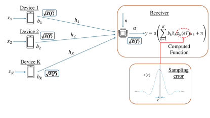
Figure 1: OTA computing model with sampling error.

II-C OTA Transmission under Sampling Error and ISI

Without loss of generality, we assume that the target function is the sum of all transmitted data. In this case, no pre- or post-processing functions are needed, except for appropriate power allocation of the participating devices. Let $b_{k}\in\mathbb{C}$ be the transmit equalization factor at the $k$-th device such that $|b_{k}|^{2}$ denotes the transmit power, $\arg\{b_{k}\}$ denotes the phase of the transmit signal and the transmitted signal of the $k$-th device in time is given as $x_{k}b_{k}z(t)$. Similarly, $a\in\mathbb{C^{*}}$ denotes the receiver gain factor. All transmitting devices are assumed to have a common maximum power magnitude $P_{\mathrm{max}}$, so that $|b_{k}|^{2}E\leq P_{\mathrm{max}}$ for all $k\in\mathcal{K}$, where $E=\int_{-\infty}^{\infty}|z(t)|^{2}\mathrm{d}t$ is the waveform energy. This constraint can be equivalently written as $|b_{k}|\leq\sqrt{P}$, where $P=P_{\mathrm{max}}/E$. Due to the perfect CSI availability, the phase of $b_{k}$ can always be chosen in such a way that the phase shift introduced by the fading is always eliminated. Thus, we consider that the receiver gain, the transmit power, and the channel coefficients are all real numbers, i.e., $a,b_{k},h_{k}\in\mathbb{R},\,\,\forall k\in\mathcal{K}$.

For our analysis, we consider that the received signal is subject to two major errors, namely the time sampling error and ISI. For the time sampling error, $\epsilon=t/T$, we assume that it follows a Gaussian distribution centered around the ideal sampling time [33] and it has variance $\sigma_{\epsilon}^{2}$, hence $\epsilon\sim\mathcal{N}(0,\sigma_{\epsilon}^{2})$. If the sampling error is the only imperfection at the receiver, the received signal can be described as

$$\hat{y}=a\left(\sum_{k=1}^{K}x_{k,0}z_{k}(\epsilon T)b_{k}h_{k}+n\right).$$ (6)

It should be highlighted that (6) corresponds to the case of flat-frequency channel fading. On the other hand, if the time sampling error coexists with ISI, the received signal is given as

$$\hat{y}_{\mathrm{ISI}} =a\left(\sum_{k=1}^{K}x_{k,0}z_{k}(\epsilon T)b_{k}h_{k,0}+n\right)$$ (7)

$$\quad+a\underbrace{\left(\sum_{\begin{subarray}{c}q=-\frac{\mu}{2}\\ q\neq 0\end{subarray}}^{\frac{\mu}{2}}\sum_{k=1}^{K}x_{k,q}z_{k}(T(q+\epsilon))b_{k}h_{k,q}\right)}_{\text{ISI terms}},$$

where $\mu$ is assumed to be even and denotes the number of ISI symbols affecting the currently transmitted symbol, while $h_{k,q}$ is the channel coefficient of the symbol $x_{k,q}$, which is transmitted at the $q$-th time instance relative to the current time, denoted by $t=0$ for convenience. It is also assumed that $t=0$ corresponds to the ideal sampling time. Note that in both cases the ideally received signal is given by

$$r=\sum_{k=1}^{K}x_{k,0}.$$ (8)

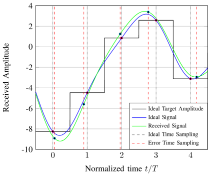
Figure 2: Signal amplitude of the target signal (8) and received signal (7) with sampling error with $\sigma_{\epsilon}=0.1$ for RC waveform of $\alpha=0.3$ in the absence of noise. The sampling instances for each case are depicted as bullet points. For the rest of the selected parameters, see Section V.

III Theoretical Analysis

In this section, we theoretically investigate the MSE of OTA computing between the ideal and actual received signal for both the RC and the BTRC waveforms. To this end, both cases of time sampling error and ISI are considered, while the optimal power allocation for any waveform during the OTA transmission is also extracted.

III-A OTA Computing under Time Sampling Error

By definition, ideal sampling of any waveform occurs exactly at intervals of symbol period $T$. Since we assume that ideal sampling occurs at $t=0$, it is clear that introducing the sampling error $\epsilon$ will lead to (6) and (8). Consequently, the MSE in this scenario can be expressed as

$$\mathrm{MSE}(a,\bm{b})=\mathbb{E}_{\epsilon}\left[\sum_{k=1}^{K}\big{(}az_{k}(\epsilon T)b_{k}h_{k}-1\big{)}^{2}+\sigma^{2}a^{2}\right],$$ (9)

where the expectation w.r.t. $x_{k},\,\forall k\in\mathcal{K}$, and $n$ have been calculated and $\bm{b}=[b_{1},\cdots,b_{K}]$ is the transmission power vector of all users. To study the performance of the MSE as described by (9), we have to first calculate the statistics of the waveform w.r.t. the sampling error. In order to simplify this calculation we consider a geometric series based approximation of the fraction term of the expression for RC in (3), which allows us to write

$$\frac{1}{1-4\alpha^{2}\epsilon^{2}}=\sum_{n=0}^{\infty}(4\alpha^{2}\epsilon^{2})^{n}=1+4\alpha^{2}\epsilon^{2}+\mathcal{O}(16\alpha^{4}\epsilon^{4}),$$ (10)

where $\mathcal{O}(\cdot)$ denotes the summary of the least-significant terms which can be considered negligible. The first equality holds due to the convergence of the geometric series whenever $\epsilon<0.5$ and the approximation is strong due to the small values of the roll-off factor and the sampling error leading to negligible values as the powers of the sampling error $\epsilon$ increase.

Thus, the mean amplitude, $\bar{\epsilon}_{1}$, and the mean squared amplitude, $\bar{\epsilon}_{2}$, at the moment of sampling can be strongly approximated as described by the following lemma.

Lemma 1

The mean amplitude value and the mean squared amplitude value of the transmitted OTA signal at $t=0$ are strongly approximated by

$$\bar{\epsilon}_{1}=1+\sum_{m=1}^{\infty}\kappa_{m}\sigma_{\epsilon}^{2m}(2m-1)!!+4\alpha^{2}\sum_{m=0}^{\infty}\kappa_{m}\sigma_{\epsilon}^{2m+2}(2m+1)!!,$$ (11)

where $\kappa_{m}$ denotes the coefficients given as

$$\kappa_{m}=\sum_{n=0}^{m}\frac{(-1)^{m}\pi^{2m}\alpha^{2(m-n)}}{(2n+1)!(2m-2n)!}$$ (12)

and

$$\bar{\epsilon}_{2} =1+\sum_{p=1}^{\infty}\lambda_{p}\sigma_{\epsilon}^{2p}(2p-1)!!+8\alpha^{2}\sum_{p=0}^{\infty}\lambda_{p}\sigma_{\epsilon}^{2p+2}(2p+1)!!$$ (13)

$$\qquad+16\alpha^{4}\sum_{p=0}^{\infty}\lambda_{p}\sigma_{\epsilon}^{2p+4}(2p+3)!!,$$

where $\lambda_{p}$ denotes the coefficients given as

$$\lambda_{p}=\sum_{n=0}^{p}\sum_{l=0}^{p-n}\sum_{k=0}^{p-n-l}\frac{(-1)^{p}\pi^{2p}\alpha^{2(p-l-n)}}{(2n+1)!(2l+1)!(2k)!(2(p-n-l-k))!}\!.$$ (14)

Proof:

The proof is presented in Appendix A. ∎

Then, taking the expected value of (9) w.r.t. the sampling error $\epsilon$ occurring in the OTA computing signal, it is straightforward to prove that the MSE under time sampling error is given as

$$\mathrm{MSE}(a,\bm{b})=\sum_{k=1}^{K}\left(\left(ab_{k}h_{k}\right)^{2}\bar{\epsilon}_{2}+1\right)-2\sum_{k=1}^{K}ab_{k}h_{k}\bar{\epsilon}_{1}+\sigma^{2}a^{2}.$$ (15)

It is important to emphasize that the following power policy allocation technique is not restricted by the use of the approximations given in (11) and (13) and can be used by numerically calculating $\bar{\epsilon}_{1}=\mathbb{E}_{\epsilon}[z_{k}(\epsilon T)]$ and $\bar{\epsilon}_{2}=\mathbb{E}_{\epsilon}[z_{k}^{2}(\epsilon T)]$. However, the strong approximation in (15) shows interest because it allows a direct calculation of the roll-off factors effect on the MSE in contrast to the numerical approach, meaning that it can also be used to solve optimization problems that would include the roll-off factor as part of the optimization variables, for instance in joint MSE-bandwidth problems

The MSE in (15) can now be minimized by finding the optimal power allocation of the OTA transmission. This problem is formulated as

$$\begin{array}[]{ll}\mathop{\mathrm{min}}\limits_{a,\bm{b}}&\mathrm{MSE}(a,\bm{b})\\ \,\,\textbf{s.t.}&\mathrm{C}_{1}:b_{k}\leq\sqrt{P},\ \forall k\in\mathcal{K}.\end{array}$$ (P1)

The Lagrangian can be written as

$$\mathcal{L}=\mathrm{MSE}(a,\bm{b})+\sum_{k=1}^{K}\lambda_{k}(b_{k}-\sqrt{P})$$ (16)

where $\lambda_{k}$ are the Lagrange multipliers.

By using the Karush-Kuhn-Tucker (KKT) conditions, the optimal solution must satisfy the following:

$$\frac{\partial\mathcal{L}}{\partial a}=0,\frac{\partial\mathcal{L}}{\partial b_{k}}=0,\forall k\in\mathcal{K}$$ (17)

and

$$\lambda_{k}(b_{k}-\sqrt{P})=0,\forall k\in\mathcal{K},$$ (18)

which equivalently leads to

$$\frac{\partial\mathrm{MSE}(a,\bm{b})}{\partial b_{k}}=0\Rightarrow b_{k}=\bar{\epsilon}_{1}/(ah_{k}\bar{\epsilon}_{2})\text{ }\mathrm{or}\text{ }b_{k}=\sqrt{P},\,\,\forall k\in\mathcal{K}.$$ (19)

Also, since $\mathrm{MSE}(a,\bm{b})$ is a convex function with respect of $b_{k}$, it holds that

$$b_{k}=\min\left\{\sqrt{P},\frac{\bar{\epsilon}_{1}}{ah_{k}\bar{\epsilon}_{2}}\right\},\forall k\in\mathcal{K}.$$ (20)

Based on (20), to further reduce the size of the set of the potential optimal points, it is sufficient to consider $K$ different cases for the values of $\lambda_{k}$. More specifically, it is noted that if there exists a device $(i+1)\in\mathcal{K}$ such that $b_{i+1}=\bar{\epsilon}_{1}/(ah_{i+1}\bar{\epsilon}_{2})$, any device $j\in\{\mathcal{K}|j>i\}$ can select the same inverse channel-like transmit power due to the ascending channel order. Thus, it holds that if $\lambda_{i+1}=0$, then $\lambda_{j}=0,\forall j>i$. Regarding the $i$-th case, by using (20), the Lagrangian simplifies to the MSE for the corresponding values of $\lambda_{k}$ and $b_{k}$, which can be written as

$$\mathcal{L}_{i}=\mathrm{MSE}_{i}(a) =a^{2}\left(\sum_{k=1}^{i}Ph^{2}_{k}\bar{\epsilon}_{2}+\sigma^{2}\right)-2a\sum_{k=1}^{i}\sqrt{P}h_{k}\bar{\epsilon}_{1}$$ (21)

$$\quad+\sum_{k=i+1}^{K}\left(1-\frac{\bar{\epsilon}_{1}^{2}}{\bar{\epsilon}_{2}}\right)+i.$$

It should be noted that for the primal feasibility conditions of (P1), i.e., $\mathrm{C}_{1}$, to be satisfied, since the channel gains have been ordered, the following must hold for the receiver gain

$$a\geq\frac{\bar{\epsilon}_{1}}{\sqrt{P}h_{i+1}\bar{\epsilon}_{2}}.$$ (22)

If (22) is satisfied, the minimum value of (21) is reached when $\partial{\mathcal{L}_{i}}/\partial a=0$, i.e.,

$$a=a_{i}=\frac{\sqrt{P}\bar{\epsilon}_{1}\sum_{k=1}^{i}h_{k}}{P\bar{\epsilon}_{2}\sum_{k=1}^{i}h^{2}_{k}+\sigma^{2}}.$$ (23)

Then, we can define the set of optimal solutions of $a$ as follows

$$\mathcal{A}=\left\{a=a_{i}\bigg{|}a_{i}\geq\frac{\bar{\epsilon}_{1}}{\sqrt{P}h_{i+1}\bar{\epsilon}_{2}},\forall i\in\mathcal{K}\right\}.$$ (24)

Observe that if $a\not\in\mathcal{A}$, it cannot be optimal since the KKT conditions described by (17) are not satisfied. Comparing the values of the sequence $\mathrm{MSE}_{i}(a_{i}),\ \forall i\in\mathcal{K},\ \forall a_{i}\in\mathcal{A}$, described by (21), we can identify the number of devices $i^{*}$ that must transmit with maximum power and is equal to

$$i^{*}=\underset{\begin{subarray}{c}1\leq i\leq K\\ a_{i}\in\mathcal{A}\end{subarray}}{\mathrm{argmin}}\,\,\{\mathrm{MSE}_{i}(a_{i})\}.$$ (25)

Then, the optimal power allocation at the devices and the receiver can be calculated by combining (25), (23) and (20) in this specific order.

III-B OTA Computing under Time Sampling Error and ISI

In limited bandwidth systems, in addition to the time sampling error, ISI is also present. Although waveforms such as RC and BTRC have relatively small amplitudes around their roots at multiples of $T$, the effect of ISI cannot be neglected, especially in multiple access schemes such as OTA computing where a large number of connected devices are present in the system. As a result, the study of ISI is important for understanding the performance of OTA computing in practice and for extracting optimal power allocation policies to mitigate its effect.

In this case the received signal is affected by the currently transmitted signal as well as earlier and later transmissions captured at time instances $t=T(q+\epsilon)$ where $q\in\{-\mu/2,\cdots,\mu/2\}$ and the received signal is given by (7). Therefore, the MSE now contains additional terms due to ISI terms and is equal to

$$\mathrm{MSE}^{\mathrm{ISI}}(a,\bm{b}) =\sum_{k=1}^{K}\left(az_{k}(\epsilon T)b_{k}h_{k}-1\right)^{2}+\sigma^{2}a^{2}$$ (26)

$$\quad+\sum_{\begin{subarray}{c}q=-\frac{\mu}{2}\\ q\neq 0\end{subarray}}^{\frac{\mu}{2}}\sum_{k=1}^{K}\left(az_{k}(T(q+\epsilon))b_{k}h_{k,q}\right)^{2},$$

where $h_{k,q}$ denotes the channel of the $k$-th device at the $q$-th time instance affected by the delay spread. Since the samples at different times are independent of each other, $\mathbb{E}_{x_{k}}[x_{k,q_{1}}x_{k,q_{2}}]=0$, whenever $q_{1}\neq q_{2}$. Then, taking the expectation w.r.t. $\epsilon$ we derive an expression similar to the one in (P1) described by

$$\mathrm{MSE}^{\mathrm{ISI}}(a,\bm{b}) \!=\!\sum_{k=1}^{K}\left(\left(ab_{k}h_{k}\right)^{2}\tilde{\epsilon}_{0}+1\right)-2\sum_{k=1}^{K}ab_{k}h_{k}\check{\epsilon}$$ (27)

$$\quad+\sum_{\begin{subarray}{c}q=-\frac{\mu}{2}\\ q\neq 0\end{subarray}}^{\frac{\mu}{2}}\sum_{k=1}^{K}\left(\left(ab_{k}h_{k,q}\tilde{\epsilon}_{q}\right)^{2}\right)+\sigma^{2}a^{2},$$

where $\tilde{\epsilon}_{q}=\mathbb{E}_{\epsilon}[z_{k}^{2}(T(q+\epsilon))]$ and $\check{\epsilon}=\mathbb{E}_{\epsilon}[z_{k}(\epsilon T)]$. In particular, for the strongest symbol interference caused by the previous and the next symbol of the currently sampled symbol, the mean values can be rigorously calculated in closed form as described by the following lemma.

Lemma 2

The mean squared amplitude of the raised cosine waveform at the time instances corresponding to $q=\pm 1$ with roll-off factor $\alpha=0$ is equal to

$$\tilde{\epsilon}_{1}=1+\sum\limits_{m=1}^{\infty}\left(\sum\limits_{n=0}^{2m}A_{n}A_{2m-n}+B_{n}B_{2m-n}\right)\sigma_{\epsilon}^{2m}(2m-1)!!,$$ (28)

and $\tilde{\epsilon}_{-1}=\tilde{\epsilon}_{1}$, where the coefficients $A_{n},B_{n}$ are given as

$$\begin{split}A_{n}&=\sum\limits_{l=\frac{n+1}{2}}^{\infty}\frac{(-1)^{l}\pi^{2l}}{(2l+1)!}\binom{2l}{n}\text{ if }n\text{ odd, }A_{n}=0\text{ if }n\text{ even }\\ B_{n}&=\sum\limits_{l=\frac{n}{2}}^{\infty}\frac{(-1)^{l}\pi^{2l}}{(2l+1)!}\binom{2l}{n}\text{ if }n\text{ even, }B_{n}=0\text{ if }n\text{ odd }.\end{split}$$ (29)

Proof:

The proof is presented in Appendix B. ∎

Moreover, the transmitting devices have no knowledge of the dynamically changing characteristics of the channel, thus they assume that the same channel is present at all time instances, i.e., each device assumes that $h_{k,q}=h_{k},\forall q$.

Considering ISI, the new optimization problem to solve can be formulated as

$$\begin{array}[]{ll}\mathop{\mathrm{min}}\limits_{a,\bm{b}}&\mathrm{MSE}^{\mathrm{ISI}}(a,\bm{b})\\ \,\,\textbf{s.t.}&\mathrm{C}_{1}:b_{k}\leq\sqrt{P},\forall k\in\mathcal{K}.\end{array}$$ (P2)

The Lagrangian of the latter can be written as

$$\mathcal{L}^{\mathrm{ISI}}=\mathrm{MSE}^{\mathrm{ISI}}(a,\bm{b})+\sum_{k=1}^{K}\lambda_{k}^{\mathrm{ISI}}(b_{k}-\sqrt{P})$$ (30)

where $\lambda^{\mathrm{ISI}}_{k}$ are the Lagrange multipliers.

By using the KKT conditions, the optimal solution must satisfy the following conditions:

$$\frac{\partial\mathcal{L}^{\mathrm{ISI}}}{\partial a}=0,\frac{\partial\mathcal{L}^{\mathrm{ISI}}}{\partial b_{k}}=0,\forall k\in\mathcal{K}$$ (31)

and

$$\lambda^{\mathrm{ISI}}_{k}\mathcal{L}^{\mathrm{ISI}}(b_{k}-\sqrt{P})=0,\forall k\in\mathcal{K}.$$ (32)

which equivalently leads to

$$\frac{\partial\mathrm{MSE}^{\mathrm{ISI}}(a,\bm{b})}{\partial b_{k}}=0\Rightarrow b_{k}=\check{\epsilon}/(ah_{k}\hat{\epsilon})\text{ }\mathrm{or}\text{ }b_{k}=\sqrt{P},\,\forall k\in\mathcal{K}.$$ (33)

Also, since $\mathrm{MSE}(a,\bm{b})$ is a convex function with respect of $b_{k}$, it holds that

$$b_{k}=\min\left\{\sqrt{P},\frac{\check{\epsilon}}{ah_{k}\hat{\epsilon}}\right\},\forall k\in\mathcal{K}.$$ (34)

For (P2), similar to (P1), based on (20), to further reduce the size of the set of the potential optimal points, it is sufficient to consider $K$ different cases for the values of $\lambda^{\mathrm{ISI}}_{k}$. More specifically, it is noted that if there exists a device $(i+1)\in\mathcal{K}$ such that $b_{i+1}=\check{\epsilon}/(ah_{i+1}\hat{\epsilon})$, any device $j\in\{\mathcal{K}|j>i\}$ can select the same inverse channel-like transmit power due to the ascending channel order. Thus, it holds that if $\lambda^{\mathrm{ISI}}_{i+1}=0$, then $\lambda^{\mathrm{ISI}}_{j}=0,\forall j>i$. Regarding the $i$-th case, by using (34), the Lagrangian simplifies to the MSE for the corresponding values of $\lambda^{\mathrm{ISI}}_{k}$ and $b_{k}$, which can be written as

$$\mathcal{L}^{\mathrm{ISI}}_{i}=\mathrm{MSE}_{i}^{\mathrm{ISI}}(a) =a^{2}\left(\sum_{k=1}^{i}Ph^{2}_{k}\hat{\epsilon}+\sigma^{2}\right)-2a\sum_{k=1}^{i}\sqrt{P}h_{k}\check{\epsilon}$$ (35)

$$\quad+\sum_{k=i+1}^{K}\left(1-\frac{\check{\epsilon}^{2}}{\hat{\epsilon}}\right)+i.$$

It should be noted that for the primal feasibility conditions of (P2), i.e., $\mathrm{C}_{1}$, to be satisfied, since the channel gains have been ordered, the following must hold for the receiver gain factor

$$\frac{\check{\epsilon}}{\sqrt{P}h_{i+1}\hat{\epsilon}}\leq a.$$ (36)

If (36) is satisfied, the minimum value of (35) is reached when $\partial{\mathcal{L}^{\mathrm{ISI}}_{i}}/\partial a=0$, i.e.,

$$a=a_{i}=\frac{\sqrt{P}\check{\epsilon}\sum_{k=1}^{i}h_{k}}{P\hat{\epsilon}\sum_{k=1}^{i}h^{2}_{k}+\sigma^{2}}.$$ (37)

Then, similar to the non-ISI case, we can define the set of optimal solutions of $a$ as follows

$$\mathcal{A}^{\mathrm{ISI}}=\left\{a=a_{i}\bigg{|}a_{i}\geq\frac{\check{\epsilon}}{\sqrt{P}h_{i+1}\hat{\epsilon}},\forall i\in\mathcal{K}\right\}.$$ (38)

Observe that if $a\not\in\mathcal{A}^{\mathrm{ISI}}$, it cannot be optimal since the KKT conditions described by (31) are not satisfied. Comparing the values of the sequence $\mathrm{MSE}^{\mathrm{ISI}}_{i}(a_{i}),\ \forall i\in\mathcal{K},\ \forall a_{i}\in\mathcal{A}^{\mathrm{ISI}}$, described by (35), we can identify the number of devices $i^{*}$ that must transmit with maximum power and is equal to

$$i^{*}=\underset{\begin{subarray}{c}1\leq i\leq K\\ a_{i}\in\mathcal{A}^{\mathrm{ISI}}\end{subarray}}{\mathrm{argmin}}\,\,\{\mathrm{MSE}^{\mathrm{ISI}}_{i}(a_{i})\}.$$ (39)

Then, the optimal power allocation at the devices and the receiver can be calculated by combining (39), (37) and (34) in this specific order.

From (34) and (37), it is evident that the MSE of an OTA transmission is affected by the statistics of the selected waveform. Therefore, it is important to emphasize that the theoretical analysis presented in this section is general and can be used to minimize the MSE for any chosen waveform, including RC and BTRC. This will be also used later to perform optimal waveform design for the OTA transmission.

IV DNN-generated Waveforms

Let $\bm{w}$ denote the weights of the DNN and $z_{\bm{w}}$ denote the output of the DNN model. To approximate a continuous waveform with the DNN, time discretization is used, i.e., each element of the output vector $z_{\bm{w}}$ corresponds to a specific time instance of the desired continuous waveform. Moreover, in practice, a windowed version of a waveform is transmitted, thus we assume that the waveform of the DNN, and the RC, BTRC waveforms expand only to a limited time window. The larger the time window, the more ISI symbols, $\mu$, are considered. To design the waveform, we utilize supervised learning by feeding as input to the DNN the vector $\bm{u}=[a,\bm{b},\bm{h},\bm{x}]\in\mathbb{R}^{3K+1}$, where $\bm{h}=[h_{1},h_{2},\cdots,h_{K}]$ denotes the channels of the devices and $\bm{x}=[x_{1,0},x_{2,0},\cdots,x_{K,0}]$ denotes the transmitted data at the current transmission time. It should be noted that we initialize the power allocation $a,\bm{b}$ with the values that correspond to the same OTA transmission without sampling error and ISI as found in [11]. The rationale behind this choice is that, as shown in Section III, finding the optimal $a,\bm{b}$ requires the statistics of the waveform, which are unknown a priori. Nevertheless, we note that to test the extracted waveform, after the DNN has converged, we obtain the optimal power allocation for the waveform through the analysis of Section III - specifically equations (34),(37),(39) - and then calculate its MSE. It should be noted that this iterative procedure is performed only once. An alternating optimization inspired method was also tested, where the optimal values of $a,\bm{b}$ are given as input to the DNN which is retrained, and new values for $a,\bm{b}$ are calculated. However, this iterative alternating optimization approach offered trivial performance gains, thus it was not used.

The architecture of the designed DNN consists of three fully connected hidden layers, each consisting of multiple neurons and implementing the rectified linear unit (ReLU) activation function. The output layer consists of $N_{s}$ output nodes which are equal to the number of discretized time instances considered. Assuming that the $N_{s}$ output nodes of the DNN correspond to $\mu+1$ time periods of the generated waveform, the waveform expands in the time domain from $-(\mu+1)T/2$ to $(\mu+1)T/2$. Then, the time resolution of the waveform is $\Delta t=(\mu+1)T/(N_{s}-1)$ and the time instances correspond to $t=m\Delta t$, with $-(N_{s}-1)/2\leq m\leq(N_{s}-1)/2$ and $m\in\mathbb{Z}$. To train the DNN, a training dataset is generated, denoted as $\{\bm{u}_{d},r_{d}\}_{d\in\mathcal{D}}$, where $\mathcal{D}$ is the set of all training samples and $\bm{u}_{d}$ is the $d$-th input sample and $r_{d}=\left\lVert\bm{x}_{d}\right\rVert_{0}$ is the target value. The received signal from the generated waveform is given similarly to (7) as

$$y_{\mathrm{DNN}}[\bm{w}, \bm{u}_{d},m]=a\left(\sum_{k=1}^{K}x_{k,0}z_{k_{\bm{w}}}[m]b_{k}h_{k,0}+n\right)$$ (40)

$$+a\underbrace{\left(\sum_{\begin{subarray}{c}q=-\frac{\mu}{2}\\ q\neq 0\end{subarray}}^{\frac{\mu}{2}}\sum_{k=1}^{K}x_{k,q}z_{k_{\bm{w}}}[m+qT]b_{k}h_{k,q}\right)}_{\text{ISI terms}}.$$

It should be noted that since the channel response at different time instances is unknown, $x_{k,q},h_{k,q}$ are passed as arguments to the loss function, but cannot be considered as inputs to the DNN framework itself. However, since both draw values from known distributions, the training phase will allow the DNN to capture their general statistics.

For the DNN to generate a valid and feasible waveform, the DNN-based waveform must meet the same criteria as the waveforms studied in the literature. Therefore, it is crucial to ensure that the DNN-based waveform has the same energy as the other waveforms and that it uses the same bandwidth to ensure that the same resources in terms of energy and frequency are utilized for fairness. Both of these constraints must be included in the loss function of the DNN model to be considered. Regarding the MSE of the OTA transmission, a challenge arises due to the stochastic nature of the time sampling error. In particular, since the sampling error is random, it is not known a priori which value of the waveform should be used in (40). In essence, considering the time discretization of the DNN output, during each forward pass a random index of the DNN output should be chosen and the waveform value corresponding to this index should be used in (40). However, this approach causes the gradient of the output to be lost during the forward propagation and the DNN cannot be trained. To overcome this problem, the sampling error distribution is approximated by an equivalent probability mass function, denoted as $f_{P}[m]$, with points at the discrete time instances considered by the DNN. For practical reasons, we assume that no sampling error greater than half a period can occur, i.e., $f_{P}[m]$ is non-zero only for $-T/2\leq t\leq T/2$ or equivalently $-(N_{s}-1)/(2(\mu+1))\leq m\leq(N_{s}-1)/(2(\mu+1))$. Then, the loss function of the DNN is given by

$$\mathcal{L}_{\mathrm{MSE}}=\frac{1}{|\mathcal{D}|}\sum_{d\in\mathcal{D}}\sum_{m=-\frac{N_{s}-1}{2(\mu+1)}}^{\frac{N_{s}-1}{2(\mu+1)}}f_{P}[m]\big{(}y_{\mathrm{DNN}}[\bm{w},\bm{u}_{d},m]-r_{d}\big{)}^{2}.$$ (41)

The utilized bandwidth, as expressed by the discrete Fourier transform (DFT) of the waveform, must first be considered for the bandwidth constraint. Considering the time resolution $\Delta t$, the frequency resolution can be found equal to $\Delta f=1/((\mu+1)T)-1/((\mu+1)TN_{s})\approx 1/((\mu+1)T)$, since the number of output nodes as well as the overall studied time duration are in general large. As known, for a baseband signal like the waveforms described by (3) and (4) the utilized bandwidth is given as $W=1/(2T)$. Thus, the effect of the roll-off factor on the total bandwidth spread can be studied for a resolution step of $1/((\mu+1)T)$, with $\alpha=0$ corresponding to the $\mu/2$-th sample, since then we obtain bandwidth utilization $W=1/(2T)$, and $\alpha=1$ corresponding to the $\mu$-th sample of the DFT, since then the previous utilized bandwidth is doubled. Obviously, this has a restrictive effect on the roll-off factors that can be investigated, thus a way to increase the frequency resolution is needed. This can be achieved by applying zero-padding, which expands a signal in time to achieve the desired frequency resolution. Denoting the additional duration of the waveforms due to zero-padding as $T^{\mathrm{ZP}}$, the frequency resolution is correspondingly increased in $\Delta f^{\mathrm{ZP}}\approx 1/((\mu+1)T+T^{\mathrm{ZP}})$ which can be derived as before but using the extended time duration of the signal. In this way, the number of roll-off factors to be examined can be chosen so that the frequency resolution corresponds to the desired roll-off factor step. For example, if the examined roll-off factors have a step of $\Delta\alpha=0.1$ corresponding to a desired frequency resolution equal to $\Delta W=\Delta\alpha/(2T)$, we can choose $T^{\mathrm{ZP}}$ to satisfy

$$\frac{1}{(\mu+1)T+T^{\mathrm{ZP}}}=\frac{\Delta\alpha}{2T}\Leftrightarrow T^{\mathrm{ZP}}=\left(\frac{2}{\Delta\alpha}-\mu-1\right)T,$$ (42)

and since the symbol period $T$ corresponds to a number of $(N_{s}-1)/(\mu+1)$ samples, it is straightforward to calculate the desired number of samples needed to perform zero-padding which are denoted as $N_{s}^{\mathrm{ZP}}$ and for which $T^{\mathrm{ZP}}=N_{s}^{\mathrm{ZP}}\Delta t$ holds. Therefore, to ensure that the generated waveform has the same bandwidth utilization as the other waveforms, a constraint is applied to keep the frequency response outside the desired spectrum as close to zero as possible. Note that if the term of the parenthesis in (42) is negative then the duration of the signal is enough to capture the desired frequency resolution and no zero-padding is needed, resulting in $N_{s}^{\mathrm{ZP}}=0$. With these in mind, we use the following as part of the loss function

$$\mathcal{L}_{f}=\frac{1}{|\mathcal{D}|}\sum_{d\in\mathcal{D}}\sum_{n>N_{t}(\alpha)}^{N_{s}+N_{s}^{\mathrm{ZP}}}\big{(}\mathcal{F}(z_{\bm{w}}[m])[n]-\Gamma_{\mathrm{thr}}\big{)}^{2},$$ (43)

where $N_{t}(\alpha)$ is the DFT sample after which no bandwidth is used for a given frequency resolution, $\Gamma_{\mathrm{thr}}$ is a frequency response threshold near zero, and $\mathcal{F}(\cdot)$ denotes the DFT. For example, assuming that $\Delta\alpha=0.1$ we want to generate a waveform for $\alpha=0.3$, it would be $N_{t}(0.3)=14$ as a result of the chosen frequency resolution and the studied roll-off factor. Since the frequency resolution is $\Delta W=0.1/(2T)$, the first $11$ samples expand in a bandwidth equal to that for $\alpha=0$, and $3$ more samples are needed to get to the utilized bandwidth when $\alpha=0.3$. Therefore, for different values of the roll-off factor, $\mathcal{L}_{f}$ must be adjusted accordingly by $N_{t}(\alpha)$ to capture the used bandwidth of the waveform found by the DFT.

In addition to equal bandwidth utilization, it is important to ensure that the generated waveform has similar energy to the others for a fair comparison. The energy of the generated waveform can be calculated using Parseval’s theorem in its DFT form and is equal to

$$E_{\mathrm{DNN}}=\frac{1}{N}\sum_{n=0}^{N-1}|\mathcal{F}(z_{\bm{w}}[m])[n]|^{2},$$ (44)

where $N=N_{s}+N_{s}^{\mathrm{ZP}}$ is the total number of samples in the zero-padded version of the waveform that is extracted through (42). Then, assuming that $E$ is the target energy of another waveform to compare to and is calculated in the same way, we arrive at the following constraint, which is passed as part of the loss function

$$\mathcal{L}_{e}=\frac{1}{|\mathcal{D}|}\sum_{d\in\mathcal{D}}\big{(}E_{\mathrm{DNN}}-E\big{)}^{2}.$$ (45)

Note that, as explained in Section II, current communication systems employ a two-part waveform break between the transmitter and receiver with each part having the following frequency response $\sqrt{|\mathcal{F}(z_{\bm{w}}[m])|}$. While this does not affect (43), it does affect the form of (44), which can now be written equivalently as

$$E_{\mathrm{DNN}}=\frac{1}{N}\sum_{n=0}^{N-1}|\mathcal{F}(z_{\bm{w}}[m])[n]|.$$ (46)

Obviously, constraint (45) changes accordingly, while the MSE term in the loss function remains unchanged.

Finally, the generated waveform requires symmetry for its samples w.r.t. the ideal sampling time. To achieve this, a constraint is introduced that aims to minimize the distance between the negative and positive parts of the waveform, as follows

$$\mathcal{L}_{s}=\frac{1}{|\mathcal{D}|}\sum_{d\in\mathcal{D}}\sum_{m=1}^{\frac{N_{s}-1}{2}}\big{(}z_{\bm{w}}[m]-z_{\bm{w}}[-m]\big{)}^{2}.$$ (47)

Combining all of the above loss function components described by (41), (43), (45), and (47) yields a total training loss function that satisfies all of the required constraints and aims to minimize the weighted MSE of the received signal for more accurate OTA computing

$$\mathcal{L}_{tot}=\mathcal{L}_{\mathrm{MSE}}+M_{f}\mathcal{L}_{f}+M_{e}\mathcal{L}_{e}+M_{s}\mathcal{L}_{s}.$$ (48)

Note that $M_{f},M_{e}$ and $M_{s}$ act as penalty factors, meaning that if their corresponding constraint is violated, the training loss will increase, so that the training will take the constraint into account and learn to stay within small violation limits. The same reasoning applies to all considered constraints in order to ensure that bandwidth, energy, and symmetry violations are kept at extremely low levels, which in turn allows the generation of a waveform that has the same characteristics as RC and BTRC, but outperforms both due to the consideration of MSE in the training phase.

However, during training, the DNN will generate a different waveform for each input sample of the training dataset. Therefore, in order to generate only one waveform that shows good performance for each input sample of the dataset, during testing only, we generate a waveform by averaging all the generated output waveforms for all input samples. Since the imposed constraints in the loss function have the distributive property, this final waveform also satisfies all constraints. This final waveform is the one we plot in Section V and on which the MSE is calculated.

V Simulation Results

In this section, we present the simulation results. For all simulations, we assume that the channel fading follows the circularly symmetric complex Gaussian distribution, i.e., $h_{k}\sim\mathcal{CN}(0,1),\ \forall k\in\mathcal{K}$, and without loss of generality, the transmitted data are generated from a uniform distribution in the interval $[-\sqrt{3},\sqrt{3}]$. Unless otherwise stated, we assume that $K=20$ devices participate in the OTA transmission and that the maximum transmit power at each device is such that the transmit SNR is $P_{\mathrm{max}}/\sigma^{2}=10$ dB. We study the problem of MSE minimization for $\mu=6$ ISI symbols, which means that the time duration of the studied waveforms extends from $-3.5T$ to $3.5T$, and we are interested in generating waveforms that perform better for a roll-off factor step equal to $\Delta\alpha=0.1$, as an indicator for the effectiveness of the proposed framework while it also provides a satisfactory performance estimation for the whole range of roll-off factors.

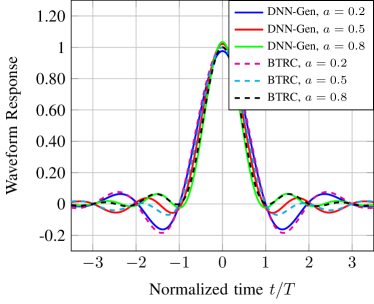
Figure 3: DNN generated waveforms for OTA computing and various roll-off factors.

V-A DNN Setup

Regarding the DNN setup, the DNN has $3$ hidden layers, each consisting of $256$ neurons, while the ReLU activation function was used. For each simulated roll-off factor of interest, a training dataset of $|\mathcal{D}|=5\times 10^{4}$ channel and data realizations is generated, while the corresponding optimal power allocation vectors were calculated according to (37) and (34). The validation and test datasets are generated in a similar manner and consist of $5\times 10^{3}$ and $5\times 10^{4}$ realizations, respectively. The Adam optimizer was used, while the DNN loss function was defined in (48). A batch size of 100 was selected, while the DNN was trained for 10 epochs.

Regarding the parameters associated with (48), the number of outputs of the proposed DNN is selected equal to $N_{s}=3501$ samples, which allows a time resolution of $\Delta t=T/500$. To achieve the desired spectral resolution, the zero-padded version of the waveform requires an additional $N_{s}^{\mathrm{ZP}}=6500$ time instances as indicated by (42). For the penalty factors, we selected $M_{f}=22.4,M_{e}=9000,M_{s}=4300$ and for the bandwidth constraint we selected $\Gamma_{\mathrm{thr}}=0.2$ as a reasonably small frequency response. Other parameter values can also be selected in the spirit of experimentation.

TABLE I: Waveform Approximation

Approximation Coefficients
	$\alpha=0.2$	$\alpha=0.5$	$\alpha=0.8$
$a_{0}$	$0.0939$	$0.1313$	$0.1360$
$a_{1}$	$0.2168$	$0.2638$	$0.2507$
$a_{2}$	$0.1841$	$0.2371$	$0.2046$
$a_{3}$	$0.2092$	$0.1676$	$0.1712$
$a_{4}$	$0.1647$	$0.1406$	$0.1315$
$a_{5}$	$0.0950$	$0.0764$	$0.0994$
$a_{6}$	$0.0121$	$0.0053$	$0.0405$
$p$	$0.6481$	$0.8378$	$0.8739$
RMSE	$3.041\times 10^{-3}$	$3.094\times 10^{-3}$	$3.132\times 10^{-3}$

V-B Generated Waveforms

In Fig. 3, waveforms for various roll-off factors are depicted, each normalized in time. These waveforms exhibit behavior reminiscent of both RC and BTRC waveforms, with larger sidelobes for smaller $\alpha$ values and steeper decay for larger $\alpha$ values. This behavior has significant implications for system performance, particularly in terms of mitigating sampling error and ISI. For small values of the roll-off factor $\alpha$, the generated waveforms illustrate slower amplitude decay. This characteristic helps mitigate the effects of sampling error, which occurs when a signal is not sampled frequently enough, resulting in inaccuracies in its representation at discrete time points. The slower decay allows the system to better accommodate such errors, thereby enhancing overall performance. Conversely, larger values of $\alpha$ increase the attenuation of ISI, which occurs when symbols in a digital communication system interfere with each other due to channel characteristics. In this scenario, the smaller amplitudes of the sidelobes in the waveforms generated for large $\alpha$ values contribute to the reduction of ISI, thereby improving the system robustness. It is noted that although the maximum values of the generated waveforms are close, they are different. This is a direct consequence of the fact that channel fading is considered during the training phase.

Figure 4: Comparison of bandwidth utilization through DFT.

In Fig. 4 the bandwidth utilization of the BTRC waveform and the DNN-generated waveforms are presented for some indicative roll-off factors. As can be observed, all waveforms have the same spectrum spread in terms of DFT samples thus, proving the efficiency of the bandwidth-related constraint introduced in the proposed DNN framework through (43). This guarantees that the extracted waveform can be useful in practice by not causing increased intercarrier interference.

To facilitate the testing of our results without the need to create the DNN architecture, we provide the curve fitting parameters for the DNN-based waveforms of 3 in Table I. This may also allow practical deployment in real communication systems, since curve fitting can generate waveforms for different roll-off factors, $\alpha$. We use sinusoidal functions for fitting due to the symmetric shape of the curves, thus the generated waveforms can be represented as follows

$$\hat{z}_{\bm{w}}(t) =a_{0}+a_{1}\cos(pt)+a_{2}\cos(2pt)+a_{3}\cos(3pt)$$ (49)

$$\quad+a_{4}\cos(4pt)+a_{5}\cos(5pt)+a_{6}\cos(6pt),$$

with $p$ and $a_{j},j\in\{0,\cdots,6\}$ being adjustable coefficients for the approximation. The root MSE (RMSE) of the fitting approximation is given in Table I as well.

V-C Performance Results

In this subsection, we evaluate the performance of the generated waveforms along with the proposed optimal power policies discussed in Section III, aiming to minimize the MSE.

V-C1 OTA under Sampling Error

In Fig. 5, we observe the closeness of the proposed approximation to the statistics of the RC waveform, as outlined in Lemma 1. Both $\bar{\epsilon}_{1}$ and $\bar{\epsilon}_{2}$, closely approximate the actual statistics of the waveform although, as the roll-off factor increases, the gap between the bounds and the actual statistics gets slightly bigger. This is expected, since a higher roll-off factor leads to a slightly larger discrepancy in the approximation of the term $1/(1-4\alpha^{2}\epsilon^{2})$. Nevertheless, the proposed approximations remain extremely tight (around $0.1\%$ and $0.3\%$ at most, respectively) and can effectively approximate the average MSE, as calculated in (P1).

Figure 5: Approximation of mean values for the RC waveform based on Lemma 1 when only sampling error with $\sigma_{\epsilon}=0.1$ occurs.

Figure 6: Waveform MSE performance for varying roll-off factor and sampling error variance $\sigma_{\epsilon}=0.1$ without the presence of ISI when there are $K=20$ devices.

In Fig. 6, we compare the MSE performance of established and DNN-generated waveforms under only the effect of sampling error. Notably, optimal performance for all waveforms is achieved for mid-range roll-off factor values, where the RC waveform performs best. This result is due to the fact that the primary goal of both the BTRC and the DNN-generated waveforms is to mitigate ISI, resulting in inferior performance when only sampling error is present. Nevertheless, the DNN-generated waveform demonstrates competitive performance across all roll-off factors, even outperforming RC and BTRC for small to medium values of $\alpha$. It should be noted that the DNN-based waveform in Fig. 5 was also trained by taking into account ISI.

V-C2 OTA under Sampling Error and ISI

Figure 7: Waveform MSE performance for varying roll-off factor and sampling error variance $\sigma_{\epsilon}=0.1$.

Figs. 7 and 8 illustrate the average MSE for varying numbers of devices in the system. It’s evident that employing the DNN-generated waveform offers satisfactory performance compared to the established RC and BTRC waveforms. Notably, this advantage remains consistent across all selected roll-off factors, particularly for mid-range values of $\alpha$, which are commonly used in practice. Moreover, despite the decreased effect of ISI when increasing the roll-off factor, the choice of waveform remains significant. Remarkably, the DNN-generated waveform outperforms the RC waveform, despite the latter utilizing a $30\%$ larger bandwidth. Moreover, for a larger sampling error value of $\sigma_{\epsilon}=0.2$, the improvement provided by the DNN-generated waveform becomes pronounced, aiding in the convergence of the MSE curve. In addition, for small roll-off factor values, the strong effect of ISI leads the MSE to increase regardless of the waveform. Thus, achieving optimal performance requires considering both roll-off factor and waveform selection to reduce the MSE.

Figure 8: Waveform MSE performance for varying roll-off factor and sampling error variance $\sigma_{\epsilon}=0.2$.

TABLE II: MSE Improvement Table

MSE Performance Gain ($\%$)
	$\sigma_{\epsilon}=0.1$		$\sigma_{\epsilon}=0.2$
	BTRC	RC	BTRC	RC
$\alpha=0.1$	$2.16$	$4.27$	$4.09$	$6$
$\alpha=0.2$	$5.65$	$12.39$	$7.20$	$13.38$
$\alpha=0.3$	$3.38$	$13.14$	$9.45$	$19.95$
$\alpha=0.4$	$5.95$	$15.96$	$12$	$25.31$
$\alpha=0.5$	$8.82$	$21.06$	$14.54$	$29.56$
$\alpha=0.6$	$5.62$	$19.68$	$13.15$	$30.97$
$\alpha=0.7$	$5.78$	$18.66$	$12.88$	$31.31$
$\alpha=0.8$	$2.49$	$15.73$	$9.36$	$29.08$
$\alpha=0.9$	$1.76$	$12.58$	$7.59$	$26.14$
$\alpha=1.0$	$2.16$	$8.29$	$4.69$	$20.84$

Table II presents the percentage improvement gain of DNN-generated waveforms over their RC and BTRC counterparts for various roll-off factors and sampling errors. The DNN-based waveforms demonstrate significant gains, particularly for mid-range roll-off factors. This is reasonable as waveforms in this range retain relatively large sidelobe amplitudes, resulting in a greater impact of ISI on the average MSE. Conversely, for large roll-off factors, the ISI effect diminishes due to the waveform having smaller sidelobes, while the DNN’s ability to generate higher-gain waveforms is constrained by bandwidth resolution limitations for small roll-off factors. Nonetheless, in practical applications where spectrum allocation matters, mid-range roll-off factors are common. In such cases, DNN-generated waveforms exhibit significant performance gains, making them a good alternative to established waveforms in the literature.

In Figs. 9 and 10, we examine the MSE performance as the transmit SNR varies. Typically, lower SNRs result in larger MSE due to significant noise effect in addition to ISI. However, we observe that as the SNR increases, the MSE decreases, with the DNN-generated waveform consistently outperforming both RC and BTRC across the entire SNR range of 0 to 20 dB. This demonstrates the robustness of the proposed approach to changes in transmit power and noise levels. Notably, despite increasing SNR, for small roll-off factors, the impact of ISI remains dominant, outweighing the benefits of power increase. This behavior arises from the fact that increased power can worsen ISI, mitigating potential performance gains at the ideal time sampling instance. Nevertheless, the DNN-generated waveform exhibits faster convergence behavior compared to the other waveforms, which is crucial for practical OTA applications.

Figure 9: Waveform MSE performance for varying roll-off factor and sampling error variance $\sigma_{\epsilon}=0.1$.

Figure 10: Waveform MSE performance for varying roll-off factor and sampling error variance $\sigma_{\epsilon}=0.2$.

Finally, another important observation drawn from the presented diagrams relates to the magnitude of the average MSE caused by ISI. Comparing these figures, specifically when there are 20 devices ($K=20$) and the transmit SNR is 10 dB, it is visible that the average MSE is considerably greater (around $60-70\%$) when ISI occurs. Also, under ISI the average MSE is heavily dependent on the choice of the roll-off factor. In contrast, under only time sampling error, the MSE is almost the same for all roll-off factor values.

VI Conclusions

Our study provides a practical examination of OTA computing performance considering time sampling error and ISI. We derived the theoretical MSE for the OTA transmission and established optimal power allocation strategies to minimize the MSE. Additionally, we introduced a novel DNN-based method for waveform design, integrating power, bandwidth, and design constraints into the DNN loss function. Simulation results confirmed our theoretical findings and demonstrated the superior performance of the designed waveform compared to the traditional RC and BTRC waveforms. Future research extensions could explore waveform design in a MIMO system, address imperfect CSI, or enhance the current DNN-based approach. An area for improvement lies in our method of obtaining a single waveform from the DNN output, which currently involves averaging multiple output waveforms. Exploring more sophisticated techniques for extracting a single waveform could be beneficial.

Appendix A Proof of Lemma 1

It is known that for the moments of a Gaussian random variable $X\sim\mathcal{N}(0,\sigma^{2})$ it holds that

$$\mathbb{E}_{X}[X^{m}]=\begin{cases}0,&\text{if }m\text{ is odd}\\ \sigma^{m}(m-1)!!,&\text{if }m\text{ is even},\end{cases}$$ (50)

where $(m-1)!!=1\cdots(m-3)(m-1)$ is the double factorial.

Let $g(\epsilon)=\mathrm{sinc}(\epsilon)\cos(\pi\alpha\epsilon)$ be the raised cosine waveform without the denominator term, $1-(2a\epsilon)^{2}$, in (3) which is strongly approximated by (10). Using the Taylor expansion of the $\mathrm{sinc}$ and $\cos$ functions, we can write

$$g(\epsilon) =\left(\sum_{n=0}^{\infty}\frac{(-1)^{n}(\pi\epsilon)^{2n}}{(2n+1)!}\right)\left(\sum_{k=0}^{\infty}\frac{(-1)^{k}(\pi\alpha\epsilon)^{2k}}{2k!}\right)$$ (51)

$$=\sum_{m=0}^{\infty}\underbrace{\sum_{n=0}^{m}\frac{(-1)^{m}\pi^{2m}\alpha^{2(m-n)}}{(2n+1)!(2m-2n)!}}_{\kappa_{m}}\epsilon^{2m},$$

where $m=n+k$. With the same technique, we can also write

$$g^{2}(\epsilon) =\left(\sum_{n=0}^{\infty}\frac{(-1)^{n}(\pi\epsilon)^{2n}}{(2n+1)!}\right)\left(\sum_{m=0}^{\infty}\frac{(-1)^{m}(\pi\epsilon)^{2m}}{(2m+1)!}\right)$$ (52)

$$\quad\times\left(\sum_{k=0}^{\infty}\frac{(-1)^{k}(\pi\alpha\epsilon)^{2k}}{2k!}\right)\left(\sum_{l=0}^{\infty}\frac{(-1)^{l}(\pi\alpha\epsilon)^{2l}}{2l!}\right)$$

$$=\sum_{p=0}^{\infty}\underbrace{\sum_{n=0}^{p}\sum_{l=0}^{p-n}\sum_{k=0}^{p-n-l}\tfrac{(-1)^{p}\pi^{2p}\alpha^{2(p-l-n)}}{(2n+1)!(2l+1)!(2k)!(2(p-n-k-l))!}}_{\lambda_{p}}\epsilon^{2p}$$

with $p=n+m+k+l$. Then, using (50), (51) and (10), for the mean value of the waveform amplitude $\bar{\epsilon}_{1}=\mathbb{E}_{\epsilon}[g(\epsilon)(1+4\alpha^{2}\epsilon^{2})]$, it holds that

$$\bar{\epsilon}_{1}=\sum_{m=0}^{\infty}\!\kappa_{m}\!\left(\!\frac{1}{\sqrt{2\pi\sigma_{\epsilon}^{2}}}\int_{-\infty}^{\infty}\epsilon^{2m}(1+4\alpha^{2}\epsilon^{2})e^{-\frac{\epsilon^{2}}{2\sigma_{\epsilon}^{2}}}\mathrm{d}\epsilon\right)$$ (53)

and (11) follows. Similarly, using (50), (52) and (10), for the mean squared amplitude $\bar{\epsilon}_{2}=\mathbb{E}_{\epsilon}[g^{2}(\epsilon)(1+4\alpha^{2}\epsilon^{2})^{2}]$, we obtain

$$\bar{\epsilon}_{2}=\sum_{p=0}^{\infty}\lambda_{p}\left(\frac{1}{\sqrt{2\pi\sigma_{\epsilon}^{2}}}\int_{-\infty}^{\infty}\epsilon^{2p}(1+4\alpha^{2}\epsilon^{2})^{2}e^{-\frac{\epsilon^{2}}{2\sigma_{\epsilon}^{2}}}\mathrm{d}\epsilon\right)$$ (54)

and (13) follows, which completes the proof.

Appendix B Proof of lemma 2

To compute the mean squared amplitude at $t=T(1+\epsilon)$, the procedure is similar to the one in Lemma 1 by expanding the $\mathrm{sinc}$ function and combining it with binomial expansion as

$$\mathrm{sinc}(1+\epsilon) =\sum_{n=0}^{\infty}\frac{(-1)^{n}\pi^{2n}}{(2n+1)!}{(1+\epsilon)}^{2n}$$ (55)

$$=\sum_{n=0}^{\infty}\frac{(-1)^{n}\pi^{2n}}{(2n+1)!}\left(\sum_{k=0}^{2n}\binom{2n}{k}\epsilon^{k}\right)$$

$$=\sum\limits_{\begin{subarray}{c}k=1,\\ k\text{ odd}\end{subarray}}^{\infty}\underbrace{\left(\sum\limits_{n=\frac{k+1}{2}}^{\infty}\frac{(-1)^{n}\pi^{2n}}{(2n+1)!}\binom{2n}{k}\right)}_{A_{k}}\epsilon^{k}$$

$$\quad+\sum\limits_{\begin{subarray}{c}k=0,\\ k\text{ even}\end{subarray}}^{\infty}\underbrace{\left(\sum\limits_{n=\frac{k}{2}}^{\infty}\frac{(-1)^{n}\pi^{2n}}{(2n+1)!}\binom{2n}{k}\right)}_{B_{k}}\epsilon^{k},$$

where $A_{k}=0$ whenever $k$ is even and $B_{k}=0$ whenever $k$ is odd, respectively. Then, according to (50), for the mean value of $\mathrm{sinc}^{2}(1+\epsilon)$ to be non-zero there are two possible combinations, i.e., odd with odd terms and even with even terms. Therefore, it holds that

$$\mathbb{E}_{\epsilon}[\mathrm{sinc}^{2}(1+\epsilon)] =\mathbb{E}_{\epsilon}\left[\left(\sum\limits_{\begin{subarray}{c}k=1,\\ k\text{ odd}\end{subarray}}^{\infty}A_{k}\epsilon^{k}\right)\left(\sum\limits_{\begin{subarray}{c}l=1,\\ l\text{ odd}\end{subarray}}^{\infty}A_{l}\epsilon^{l}\right)\right]$$ (56)

$$\quad+\mathbb{E}_{\epsilon}\left[\left(\sum\limits_{\begin{subarray}{c}k=0,\\ k\text{ even}\end{subarray}}^{\infty}B_{k}\epsilon^{k}\right)\left(\sum\limits_{\begin{subarray}{c}l=0,\\ l\text{ even}\end{subarray}}^{\infty}B_{l}\epsilon^{l}\right)\right]$$

$$=\mathbb{E}_{\epsilon}\left[\sum\limits_{\begin{subarray}{c}m=2,\\ m\text{ even}\end{subarray}}^{\infty}\left(\sum\limits_{\begin{subarray}{c}n=1,\\ n\text{ odd}\end{subarray}}^{m}A_{n}A_{m-n}\right)\epsilon^{m}\right]$$

$$\quad+\mathbb{E}_{\epsilon}\left[\sum\limits_{\begin{subarray}{c}m=0,\\ m\text{ even}\end{subarray}}^{\infty}\left(\sum\limits_{\begin{subarray}{c}n=0,\\ n\text{ even}\end{subarray}}^{m}B_{n}B_{m-n}\right)\epsilon^{m}\right],$$

which can be equivalently reduced to

$$\tilde{\epsilon}_{1}=\mathbb{E}_{\epsilon}[\mathrm{sinc}^{2}(1+\epsilon)]=\mathbb{E}_{\epsilon}\left[\sum\limits_{m=0}^{\infty}\left(\sum\limits_{n=0}^{2m}A_{n}A_{2m-n}+B_{n}B_{2m-n}\right)\epsilon^{2m}\right],$$ (57)

from which we can conclude (28) using (50) and $B_{0}^{2}=1$.

Then, due to the symmetry of the Gaussian random variable with zero mean, it holds that

$$\mathbb{E}_{\epsilon}[\mathrm{sinc}^{2}(-1+\epsilon)]=\mathbb{E}_{\epsilon}[\mathrm{sinc}^{2}(-1-\epsilon)]=\mathbb{E}_{\epsilon}[\mathrm{sinc}^{2}(1+\epsilon)],$$ (58)

where the second equality holds due to the fact that $\mathrm{sinc}^{2}(\cdot)$ is an even function. Thus, $\tilde{\epsilon}_{1}=\tilde{\epsilon}_{-1}$, which completes the proof.

References

- [1] N. G. Evgenidis, N. A. Mitsiou, V. I. Koutsioumpa, S. A. Tegos, P. D. Diamantoulakis, and G. K. Karagiannidis, “Multiple access in the era of distributed computing and edge intelligence,” 2024. [Online]. Available: https://arxiv.org/abs/2403.07903
- [2] G. Zhu, J. Xu, K. Huang, and S. Cui, “Over-the-air computing for wireless data aggregation in massive IoT,” IEEE Wireless Commun., vol. 28, no. 4, pp. 57–65, Aug. 2021.
- [3] M. Gastpar, “Uncoded transmission is exactly optimal for a simple gaussian sensor network,” IEEE Trans. Inf. Theory, vol. 54, pp. 5247–5251, Nov. 2008.
- [4] A. Assalini and A. Tonello, “Improved nyquist pulses,” IEEE Commun. Lett., vol. 8, no. 2, pp. 87–89, Feb. 2004.
- [5] N. Beaulieu, C. Tan, and M. Damen, “A “better than” nyquist pulse,” IEEE Commun. Lett., vol. 5, no. 9, pp. 367–368, Sep. 2001.
- [6] F. Molinari, S. Stanczak, and J. Raisch, “Exploiting the superposition property of wireless communication for average consensus problems in multi-agent systems,” in Proc. Eur. Control Conf. (ECC), 2018, pp. 1766–1772.
- [7] M. Goldenbaum and S. Stanczak, “Robust analog function computation via wireless multiple-access channels,” IEEE Trans. Commun., vol. 61, no. 9, pp. 3863–3877, Sep. 2013.
- [8] M. Goldenbaum, H. Boche, and S. Stanczak, “Nomographic functions: Efficient computation in clustered gaussian sensor networks,” IEEE Trans. Wireless Commun., vol. 14, pp. 2093–2105, Apr. 2015.
- [9] M. Goldenbaum, H. Boche, and S. Stańczak, “Analyzing the space of functions analog-computable via wireless multiple-access channels,” in Proc. 8th Int. Symp. Wireless Commun. Syst., Nov 2011, pp. 779–783.
- [10] P. S. Bouzinis, N. G. Evgenidis, N. A. Mitsiou, S. A. Tegos, P. D. Diamantoulakis, and G. K. Karagiannidis, “Universal function approximation through over-the-air computing: A deep learning approach,” IEEE Open J. Commun. Soc., vol. 5, pp. 2958–2967, Apr. 2024.
- [11] W. Liu, X. Zang, Y. Li, and B. Vucetic, “Over-the-air computation systems: Optimization, analysis and scaling laws,” IEEE Trans. Wireless Commun., vol. 19, no. 8, pp. 5488–5502, Aug. 2020.
- [12] X. Cao, G. Zhu, J. Xu, Z. Wang, and S. Cui, “Optimized power control design for over-the-air federated edge learning,” IEEE J. Sel. Areas Commun, vol. 40, no. 1, pp. 342–358, Jan. 2022.
- [13] N. G. Evgenidis, V. K. Papanikolaou, P. D. Diamantoulakis, and G. K. Karagiannidis, “Over-the-air computing with imperfect CSI: Design and performance optimization,” IEEE Trans. Wireless Commun., pp. 1–1, 2023.
- [14] P. S. Bouzinis, N. A. Mitsiou, P. D. Diamantoulakis, D. Tyrovolas, and G. K. Karagiannidis, “Intelligent over-the-air computing environment,” IEEE Wireless Commun. Lett., vol. 12, no. 1, pp. 134–137, Jan. 2023.
- [15] T. Jiang and Y. Shi, “Over-the-air computation via intelligent reflecting surfaces,” in Proc. IEEE Global Commun. Conf. (GLOBECOM), 2019, pp. 1–6.
- [16] W. Fang, Y. Jiang, Y. Shi, Y. Zhou, W. Chen, and K. B. Letaief, “Over-the-air computation via reconfigurable intelligent surface,” IEEE Trans. Commun., vol. 69, no. 12, pp. 8612–8626, Dec. 2021.
- [17] M. Fu, Y. Zhou, Y. Shi, W. Chen, and R. Zhang, “UAV aided over-the-air computation,” IEEE Trans. Wireless Commun., vol. 21, no. 7, pp. 4909–4924, Jul. 2022.
- [18] X. Zhai, X. Chen, J. Xu, and D. W. Kwan Ng, “Hybrid beamforming for massive MIMO over-the-air computation,” IEEE Trans. Commun., vol. 69, no. 4, pp. 2737–2751, Apr. 2021.
- [19] G. Zhu and K. Huang, “MIMO over-the-air computation for high-mobility multimodal sensing,” IEEE Internet Things J., vol. 6, no. 4, pp. 6089–6103, Aug. 2019.
- [20] X. Li, F. Liu, Z. Zhou, G. Zhu, S. Wang, K. Huang, and Y. Gong, “Integrated sensing, communication, and computation over-the-air: MIMO beamforming design,” IEEE Trans. Wireless Commun., vol. 22, no. 8, pp. 5383–5398, Aug. 2023.
- [21] X. Zhai, X. Chen, and Y. Cai, “Power minimization for massive MIMO over-the-air computation with two-timescale hybrid beamforming,” IEEE Wireless Commun. Lett., vol. 10, no. 4, pp. 873–877, Apr. 2021.
- [22] D. Wen, G. Zhu, and K. Huang, “Reduced-dimension design of mimo over-the-air computing for data aggregation in clustered IoT networks,” IEEE Trans. Wireless Commun., vol. 18, no. 11, pp. 5255–5268, Nov. 2019.
- [23] L. Chen, N. Zhao, Y. Chen, F. R. Yu, and G. Wei, “Over-the-air computation for IoT networks: Computing multiple functions with antenna arrays,” IEEE Internet Things J., vol. 5, no. 6, pp. 5296–5306, Dec. 2018.
- [24] G. Zhu, Y. Du, D. Gündüz, and K. Huang, “One-bit over-the-air aggregation for communication-efficient federated edge learning: Design and convergence analysis,” IEEE Trans. Wireless Commun., vol. 20, no. 3, pp. 2120–2135, Mar. 2021.
- [25] K. Yang, T. Jiang, Y. Shi, and Z. Ding, “Federated learning via over-the-air computation,” IEEE Trans. Wireless Commun., vol. 19, no. 3, pp. 2022–2035, Mar. 2020.
- [26] C. Xu, S. Liu, Z. Yang, Y. Huang, and K.-K. Wong, “Learning rate optimization for federated learning exploiting over-the-air computation,” IEEE J. Sel. Areas Commun., vol. 39, no. 12, pp. 3742–3756, Dec. 2021.
- [27] X. Fan, Y. Wang, Y. Huo, and Z. Tian, “Joint optimization of communications and federated learning over the air,” IEEE Trans. Wireless Commun., vol. 21, no. 6, pp. 4434–4449, Jun. 2022.
- [28] M. Mohammadi Amiri and D. Gunduz, “Machine learning at the wireless edge: Distributed stochastic gradient descent over-the-air,” IEEE Trans. Signal Process., vol. 68, pp. 2155–2169, Mar. 2020.
- [29] N. A. Mitsiou, P. S. Bouzinis, P. D. Diamantoulakis, R. Schober, and G. K. Karagiannidis, “Accelerating distributed optimization via over-the-air computing,” IEEE Trans. Commun., vol. 71, no. 9, pp. 5565–5579, Sep. 2023.
- [30] S. Razavikia, J. M. Barros da Silva, and C. Fischione, “Channelcomp: A general method for computation by communications,” IEEE Trans. Commun., vol. 72, no. 2, pp. 692–706, Feb. 2024.
- [31] H. Hellström, S. Razavikia, V. Fodor, and C. Fischione, “Optimal receive filter design for misaligned over-the-air computation,” in Proc. IEEE Globecom Workshops (GC Wkshps), 2023, pp. 1529–1535.
- [32] G. Turin, “An introduction to matched filters,” IRE Transactions on Information Theory, vol. 6, no. 3, pp. 311–329, Jun. 1960.
- [33] A. Papoulis, “Error analysis in sampling theory,” Proceedings of the IEEE, vol. 54, no. 7, pp. 947–955, Jul. 1966.