Poynting flux transport channels formed in polar cap regions of neutron star magnetospheres

Abstract

Context. Pair cascades in polar cap regions of neutron stars are considered to be an essential process in various models of coherent radio emissions of pulsars. The cascades produce pair plasma bunch discharges in quasi-periodic spark events. The cascade properties, and therefore also the coherent radiation, depend strongly on the magnetospheric plasma properties and vary significantly across and along the polar cap. It is furthermore still uncertain from where the radio emission emanates in polar cap region.

Aims. We investigate the generation of electromagnetic waves by pair cascades and their propagation in the polar cap for three representative inclination angles of a magnetic dipole, $0^{\circ}$, $45^{\circ}$, and $90^{\circ}$.

Methods. 2D particle-in-cell simulations that include quantum-electrodynamic pair cascades are used in a charge limited flow from the star surface.

Results. We found that the discharge properties are strongly dependent on the magnetospheric current profile in the polar cap and that transport channels for high intensity Poynting flux are formed along magnetic field lines where the magnetospheric currents approach zero and where the plasma cannot carry the magnetospheric currents. There, the parallel Poynting flux component is efficiently transported away from the star and may eventually escape the magnetosphere as coherent radio waves. The Poynting flux decreases faster with the distance from the star in regions of high magnetospheric currents.

Conclusions. Our model shows that no process of energy conversion from particles to waves is necessary for the coherent radio wave emission. Moreover, the pulsar radio beam does not have a cone structure, but rather the radiation generated by the oscillating electric gap fields directly escapes along open magnetic field lines in which no pair creation occurs.

1 Introduction

It is widely assumed that the coherent radio emission in rotation powered pulsars originates in or close to their polar cap regions where pair cascades create a dense electron-positron plasma (Sturrock, 1971; Ruderman & Sutherland, 1975; Cheng & Ruderman, 1977; Daugherty & Harding, 1982). However, the exact coherent radio emission emission mechanism, and its location remain uncertain (Melrose & Rafat, 2017; Melrose et al., 2020; Philippov & Kramer, 2022).

The polar cap pair cascades play an essential role in filling of the neutron star magnetosphere with plasma (Tomczak & Pétri, 2023), powering the plasma instabilities behind coherent radio emissions (Asseo & Melikidze, 1998; Melikidze et al., 2000; Gil et al., 2004), as well as in powering the pulsar wind (Pétri, 2022), heating the neutron star surface (Zhang & Harding, 2000; Gonzalez & Reisenegger, 2010; Köpp et al., 2023), and emission of a wide spectral range of electromagnetic waves (Hobbs et al., 2004; Daugherty & Harding, 1996; Pétri, 2019; Giraud & Pétri, 2021). Dense plasma trapped in the closed magnetic field line zone of the pulsar magnetosphere screens the electric field component parallel to the magnetic field, thus suppressing particle acceleration in this zone. There is no poloidal current flowing along closed magnetic field lines, and the plasma co-rotates with the neutron star. Along open magnetic field lines, the plasma flows away from the neutron star, forming pulsar wind. The flow of this plasma generates poloidal currents supporting the force-free structure of the pulsar magnetosphere (Goldreich & Julian, 1969). The plasma has to be constantly replenished as it is leaving the inner magnetosphere. Most of this plasma is generated in electron-positron cascades in pulsar polar caps — regions close to the magnetic poles — as first suggested by Sturrock (1971). These cascades are initiated by ultrarelativistic particles accelerated in the regions of the polar cap with strong parallel electric field called gaps. The electric field appears when the plasma can not sustain the poloidal current density, and can not provide the charge density required to maintain the twist of open magnetic field lines and the corresponding electric fields so that the magnetosphere remains force-free (Beloborodov, 2008; Timokhin, 2010; Timokhin & Arons, 2013). Particles accelerated to high energies in the gaps emit $\gamma$-ray photons that interact with the super strong magnetic field, thereby creating electron–positron pairs.

Pair creation occurs in the form of repetitive cascade events. When sufficient particles have been produced in a cascade, the motion of the plasma charges begins to support the required poloidal currents and the charge separation can sustain the required charge density. That causes the screening of the electric field and the cessation of pair creation. When the newly created plasma leaves the polar cap, the plasma density drops again, the necessary current and charge densities can not be sustained, and the discharge repeats. The cascade events in polar caps were first studied by particle-in-cell (PIC) 1D (one dimension in space) electrostatic simulations from first principles by Timokhin (2010); Timokhin & Arons (2013). The $\gamma$-ray photons in those simulations were produced by curvature radiation of the curved particle motion in the magnetosphere. It was shown that the value of the required poloidal current density strongly influences the discharge behavior and their repetition — the burst of pair creation is followed by a longer phase when the dense freshly created plasma flows into the magnetosphere, and the accelerating field is fully screened. The total pair production efficiency of polar cap cascades has been recently studied in Timokhin & Harding (2015, 2019) and it was shown that the number of produced particles does not exceed $\sim$few$\times$10⁵ per primary particle. Cruz et al. (2021b, 2022) investigated the filling of the magnetosphere by pairs using the PIC simulations, the generation of large-amplitude oscillating electrostatic waves, and the growth rates and screening times of the magnetospheric electric fields. Okawa & Chen (2024) studied pair creation and parallel electric field screening. They showed that the time-averaged power spectrum is similar to a typical pulsar radio spectrum. The $\gamma-$photon polarization during the QED cascade was considered by Song & Tamburini (2024), revealing that during the cascade, the synchrotron losses may dominate over those from curvature radiation.

The 1D electrostatic simulations of Timokhin (2010); Timokhin & Arons (2013) showed that the intermittent screening of the electric field during pair discharges generates strong superluminal electrostatic waves. It was speculated that in multi-dimensional discharges, these waves might become electromagnetic waves, with a component of the electric field perpendicular to the magnetic field $\boldsymbol{B}$. If these waves escape the plasma, they can become observable as coherent radio emission. Philippov et al. (2020) further developed this idea and proposed a novel mechanism for the generation of electromagnetic waves in the plasma during pair discharges. In this mechanism, the inhomogeneity of pair production across the magnetic field lines causes the appearance of a perpendicular (to $\boldsymbol{B}$) component of the electric field and, thus, despite all particles in the discharge moving strictly along the magnetic field lines, the discharge generates an electromagnetic mode. They performed the first 2D simulations of pair cascades and confirmed the appearance of such waves during pair discharges. They showed that the spectra of such waves are broadband, and their frequency ranges are commensurate with the observed pulsar spectra. Tolman et al. (2022) studied the damping of such waves during discharges when plasma density grows rapidly due to the ongoing pair creation. It was shown that after initially strong exponential damping, the damping of the waves becomes linear in time. That indicates that these waves could still contain enough energy when they decouple from plasma and become electromagnetic waves observed as pulsar radio emission when plasma density drops at some distance from the discharge zone. Benáček et al. (2023) studied the linear acceleration emission of the time-evolving plasma bunches by postprocessing of results from PIC simulations and found that the emission spectrum is comparable with the observed one for typical pulsars.

The radio emission mechanism suggested by Philippov et al. (2020) has been recently studied by other authors as well. Cruz et al. (2021a) studied the polar cap of an aligned pulsar using a more realistic setup than in Philippov et al. (2020) by considering cascades along diverging magnetic field lines. In their simulations, they observed two peaks in the outflowing Poynting flux of electromagnetic plasma waves that could be associated with core and conal components of pulsar radio emissions (Rankin, 1990, 1993). Bransgrove et al. (2023) performed global 2D PIC simulations of the aligned rotator’s magnetosphere and demonstrated the excitation of electromagnetic waves in pair discharges whenever they occur in the magnetosphere.

However, the details of how the pair cascades produce the observed radiation are still lacking. In addition, it is an open question how the generated Poynting flux and hence the properties of the produced radio waves are influenced by the local kinetic plasma properties and the global magnetospheric environment.

In this paper, we focus on how the pulsar inclination angle, the angle between the pulsar’s magnetic moment and its angular velocity of rotation, and thus the magnetospheric current profile across the polar cap, influences the discharges, the production of plasma bunches, and the Poynting flux of electromagnetic waves that are generated in the discharges. We investigate the time evolution of pair cascades in the polar cap region under the assumption of charge limited flow, when particles can freely leave neutron star surface (Arons & Scharlemann, 1979) using kinetic and relativistic PIC simulations from first principles. In our model the discharges are driven by the magnetospheric currents and their profile across the polar cap, the latter being known from global magnetospheric general-relativistic force-free simulations that include a return current.

This paper is structured as follows. In Section 2, we discuss the plasma and numerical setup of the particle in cell simulations. Section 3 describes the cascade evolution and shows the properties of the cascade events after reaching quasi-periodic state. We discuss the cascade and radiation properties in Section 4 and state the main conclusions about the Poynting flux properties in Section 5.

2 Methods

2.1 Polar Cap Model

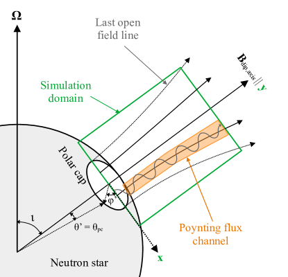
Figure 1: Scheme of the neutron star polar cap in the considered model. Not to scale.

Table 1: Parameters for the star and simulation.

Parameter	Values
Dipole inclination $\iota$	0∘	45∘	90∘
Dipole magnetic field $B_{\mathrm{dip,axis}}$	1012 G
Star rotation period $P$	0.25 s
Star mass $M_{\star}$	1.5 Ms
Star radius $R_{\star}$	12 km
Domain size $L_{x}$	11 000$\Delta_{\mathrm{x}}$	11 000$\Delta_{\mathrm{x}}$	9 000$\Delta_{\mathrm{x}}$
Domain size $L_{y}$	12000$\Delta_{\mathrm{x}}$
Grid cell size $\Delta_{\mathrm{x}}$	13.4 cm
Initial plasma skin depth $d_{\mathrm{e}}(n_{0})/\Delta_{\mathrm{x}}$	14.93
Simulation time step $\Delta t$	0.2011 ns
Simulation time steps $T/\Delta t$	150 000
Polar cap angle $\theta_{\mathrm{pc}}$, Eq. 1	2.01∘	2.15∘	2.20∘
Polar cap transition angle $\Delta\theta/\theta_{\mathrm{pc}}$	0.01
Current profile $j_{\parallel}/j_{\mathrm{GJ}}$	Eq. 5, Fig. 2
Particle decay threshold $\gamma_{\mathrm{thr}}$	$2\times 10^{7}$
Secondary particle $\gamma_{\mathrm{sec}}$	$1\times 10^{4}$
Friedman filter $\theta_{\mathrm{Fr}}$	0.1
Initial macro-particle density representing $n_{0}$	2 PPC
Initial and injection particle velocity $u_{\mathrm{0}}/c$	0.1
Initial density closed lines $n_{\mathrm{closed}}$	$50\,n_{0}$
Absorbing boundary condition width $l_{\mathrm{abc}}$	40$\Delta_{\mathrm{x}}$

We assume a spherical neutron star with a mass $M_{\star}=1.5\,M_{\mathrm{s}}$, where $M_{\mathrm{s}}$ is the solar mass, a radius $R=12$ km, and a rotation period $P=0.25$ s. We denote the dipole magnetic field as $\boldsymbol{B}_{\mathrm{dip}}$ and the magnetic field in the dipole axis at the star surface as $\boldsymbol{B}_{\mathrm{dip,axis}}=\boldsymbol{B}_{\mathrm{dip}}(\iota,R_{\star})$. The dipole axis has an inclination angle $\iota$ to the star rotational axis $\boldsymbol{\Omega}$. We study three dipole inclinations of $\iota=0^{\circ},45^{\circ},$ and $90^{\circ}$. The summary of all simulation parameters is in Table 1.

The polar cap has a radius that is defined by the ‘last open magnetic field line’ (Gralla et al., 2017)

$$\alpha_{\mathrm{pc}}(\iota)=\sqrt{\frac{3}{2}}\mu\Omega\left(1+\frac{1}{5}\sin^{2}\iota\right),$$ (1)

where $\Omega=2\pi/P$ is the star angular velocity and $\mu$ is the dipole magnetic moment. For the considered inclinations $\iota$, the last open magnetic field lines correspond to polar cap angles

$$\theta_{\mathrm{pc}}(\iota)\equiv\arcsin\sqrt{\frac{\alpha_{\mathrm{pc}}R_{\star}}{\mu}}\approx 2.01^{\circ},2.15^{\circ},\mathrm{and}\,2.20^{\circ}.$$

The polar cap is described in spherical coordinates $(\theta,\varphi,r)$ centered at the star center. The polar angle $\theta$ is measured from the magnetic dipole axis, and the azimuthal angle $\varphi$ is denoted as in Figure 1. In addition, we assume a transition angle $\theta\in(\theta_{\mathrm{pc}},\theta_{\mathrm{pc}}+\Delta\theta)$ between the closed and open field lines, with $\Delta\theta=0.01\,\theta_{\mathrm{pc}}$.

The magnetic field is constructed as a composition of two fields

$$\boldsymbol{B}(\boldsymbol{x},t)=\boldsymbol{B}_{\mathrm{dip}}(\boldsymbol{x})+\delta\boldsymbol{B}(\boldsymbol{x},t),$$ (2)

where $\delta\boldsymbol{B}$ is the local space- and time-varying field, and $\boldsymbol{B}_{\mathrm{dip}}$ is the external dipole field that does not change its structure in the polar cap in time. Close to the star, this approximation is valid as the light cylinder distance is $Pc/2\pi\approx 10^{3}R_{\star}$.

2.2 Particle-in-Cell Simulations

Because global kinetic magnetospheric simulations on current supercomputers do not resolve the kinetic scales of a typical pulsar polar cap, we investigate the polar cap in a local frame co-rotating with the neutron star. The plasma is described at kinetic scales using a fully-kinetic, relativistic, and electromagnetic particle-in-cell (PIC) code. We utilize the 2D3V version of the code ACRONYM with a rectangular grid (Kilian et al., 2012).

We use the fourth order M24 finite-difference time-domain (FDTD) method proposed by Greenwood et al. (2004) for computation on the Yee lattice to efficiently describe the wave dispersion properties of relativistic plasmas. We combine the field solver with the Friedman (1990) low-pass filtering method with the Friedman parameter $\theta_{\mathrm{Fr}}=0.1$ to weakly suppress the numerical Cerenkov radiation. For the current deposition, we utilize the Esirkepov (2001) current-conserving deposition scheme with a fourth-order “weighting with time-step dependency” (WT4) shape function of macro-particles (Lu et al., 2020). We use the Vay et al. (2011) particle pusher that was modified to advance particles in the gyro-motion approximation (Philippov et al., 2020). The approximation assumes a strict particle motion along the direction of the local magnetic field vector, and the pusher utilizes, therefore, only the parallel component of the electric field. The approach is valid because the particles are assumed to lose their kinetic energy perpendicular to the magnetic field in a much shorter time than one simulation time step. The particle pusher assumes that the gravitational force of the neutron star has only a weak impact on non-relativistic particles.

The simulation uses a uniform rectangular grid of size $L_{\mathrm{x}}\times L_{\mathrm{y}}$. For a scheme, please see Figure 1. The length $L_{\mathrm{y}}$ is fixed to $12\,000\Delta_{\mathrm{x}}$ along the dipole axis, where $\Delta_{\mathrm{x}}=13.4$ cm is the grid size. The length $L_{\mathrm{x}}$ is varied to cover the whole polar cap angle with the transition angle and the return current, giving $L_{\mathrm{x}}=11\,000\Delta_{\mathrm{x}},11\,000\Delta_{\mathrm{x}},$ and $9\,000\Delta_{\mathrm{x}}$ for $\iota=0^{\circ},45^{\circ},$ and $90^{\circ}$, respectively. For example, for $\iota=0^{\circ}$, the real size of the domain is 1474 m $\times$ 1608 m. The simulation length $L_{\mathrm{y}}$ covers larger distances than the typically assumed electric gap size of $l_{\mathrm{gap}}\simeq 50-100$ m, and maintains the scaling relations $L_{\mathrm{y}}\gg l_{\mathrm{gap}}\gg\Delta_{\mathrm{x}}$. The time step is chosen as $\Delta t=0.45\Delta_{\mathrm{x}}/c\approx 0.2011$ ns.

The simulation domain is a 2D cut through the 3D polar cap in the $\boldsymbol{\Omega}-\boldsymbol{B}_{\mathrm{dip,axis}}$ plane. In all three cases, the start of the coordinate system ($x=0$, $y=0$) is at the dipole axis below the star surface ($r\lesssim R_{\star}$). The star surface is located $\sim 70\Delta_{\mathrm{x}}\approx 9.4$ m from the simulation boundary at the dipole axis. As the surface bends, it approaches the simulation boundary to 20 grid cells, $\approx 2.7$ m, at the last open field line. The simulation $y$-axis is always parallel to $\boldsymbol{B}_{\mathrm{dip,axis}}$.

2.3 Magnetospheric Currents

We add global magnetospheric currents $j_{\mathrm{mag}}(\boldsymbol{x})$ by modifying the PIC field solver as Timokhin (2010, Appendix A)

$$\frac{\partial\boldsymbol{E}(\boldsymbol{x},t)}{\partial t}=-\left(\boldsymbol{j}(\boldsymbol{x},t)+\boldsymbol{j}_{\mathrm{mag}}(\boldsymbol{x})\right)+c(\nabla\times\delta\boldsymbol{B}(\boldsymbol{x},t)).$$ (3)

The term $(\nabla\times\delta\boldsymbol{B})$ only contains the time-evolving magnetic field. The current density $j(\boldsymbol{x},t)$ is caused by the plasma motion. The term $\boldsymbol{j}_{\mathrm{mag}}(\boldsymbol{x})$ in Eq. 3 represents the current density “demanded” by the magnetosphere — the current density necessary to support the twist of magnetic field lines in the force-free magnetosphere.

We assume the current $\boldsymbol{j}_{\mathrm{mag}}$ is always parallel to the dipole magnetic field

$$\boldsymbol{j}_{\mathrm{mag}}(\boldsymbol{x})=j_{\parallel}(\boldsymbol{x})\frac{\boldsymbol{B}_{\mathrm{dip}}(\boldsymbol{x})}{|\boldsymbol{B}_{\mathrm{dip}}(\boldsymbol{x})|}.$$ (4)

We express the magnetospheric parallel current $j_{\parallel}$ separately for the open and closed magnetic field lines. In open field lines, it is expressed as an analytical fit of the currents across the polar cap that was found by Gralla et al. (2017) and Lockhart et al. (2019) in general-relativistic force-free simulations

$$\frac{j_{\parallel}(\alpha,\beta)}{j_{\mathrm{GJ}}}=\frac{\pm 1}{\pi\sqrt{\Upsilon}}\left\{J_{0}\left(2\arcsin\sqrt{\frac{\alpha}{\alpha_{\mathrm{pc}}}}\right)\cos\iota\right.\\ \mp\left.J_{1}\left(2\arcsin\sqrt{\frac{\alpha}{\alpha_{\mathrm{pc}}}}\right)\cos\beta\sin\iota\right\},\qquad\alpha<\alpha_{0},$$ (5)

where we normalize the current to the local Goldreich–Julian current (Goldreich & Julian, 1969) for an aligned pulsar

$$j_{\mathrm{GJ}}\equiv-c\rho_{\mathrm{GJ}}\left(B_{\mathrm{dip}}(\boldsymbol{x},\iota=0)\right)\equiv-\frac{\Omega B_{\mathrm{dip}}(\boldsymbol{x})}{2\pi}$$ (6)

and

$$\Upsilon\approx 1-\frac{2GM_{\star}}{c^{2}}\frac{1}{r},$$ (7)

$$\alpha=\frac{\mu}{r}\sin^{2}\theta^{\prime},\qquad\beta=\varphi^{\prime},$$ (8)

is the reddening factor. The angles $(\alpha,\beta,r)$ and $(\theta^{\prime},\varphi^{\prime},r)$ are the spherical coordinates of the polar cap region referred to the dipole axis, $J_{0}$ and $J_{1}$ are the Bessel functions of the first kind, $\Upsilon$ is the reddening factor, $G$ is the gravitational constant, and $M_{\star}$ is the star mass. The $\pm$ signs in Equation 5 correspond to the north and south magnetic poles, respectively.

Our model incorporates a return current in the closed field lines so that the net magnetospheric current through the simulation vanish. The return current has a half-sine wave, and its amplitude is set to $j\sqrt{\Upsilon}/j_{\mathrm{GJ}}=6$. If the magnetospheric current Eq. 5 is non-zero on the last open field line, a part of the sinusoidal wave is truncated, thereby maintaining the smooth functional form of the current profile. The width of the return current is adjusted so that the resulting net current is zero for each simulation. For $\iota=90^{\circ}$, the net current is zero; no return current was added.

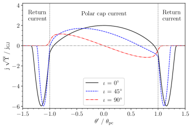
Figure 2: Magnetospheric current profile across the polar cap at the star surface for used dipole inclination angles. The currents are normalized to the Goldreich–Julian magnetospheric current density for an aligned pulsar, $j_{\mathrm{GJ}}$, and the reddening factor, $\Upsilon$.

The simulation plane is a cut across the polar cap. We define the cut for $\varphi^{\prime}=0$ as $\theta^{\prime}\geq 0$ and for $\varphi^{\prime}=\pi$ as $\theta<0$. We smooth the magnetospheric current profiles by convolution with a Gaussian function with a width of $0.04\theta_{\mathrm{pc}}$ in order to obtain a smooth transition between open and closed field lines. The resulting global magnetospheric current profiles used in simulations are shown in Figure 2.

2.4 Boundary and Initial Conditions

We assume that the initial electric field is zero in the simulation domain and that the magnetic field $B_{\mathrm{ext}}$ is given only by the dipole magnetic field. The open magnetic field lines are initially filled with $n_{0}=2$ macro-particles per cell (PPC), and the closed field lines by $n_{\mathrm{closed}}=10$ PPC, half electrons and half positrons. The macro-particles in closed field lines represent ten times more plasma particles than those in open field lines, i.e., their physical density is 50 times higher than in closed field lines. Therefore, not many macro particles are required to sustain the relatively large return current in closed field lines. The plasma in open magnetic field lines is not dense enough to fully sustain the magnetospheric currents. We implemented a linear transition in density between these regions of the angular width $\Delta\theta$. That corresponds to $\approx$$34\Delta_{\mathrm{x}}\approx 4.5$ m on the star surface. This width assures that the transition between both regions is not too steep for an appropriate representation by the simulation grid.

Initially, all particles have the Maxwell-Boltzmann distribution function with a thermal velocity of $u_{\mathrm{0}}=0.1\,c$. The particles are then accelerated by electric fields. The particles from the initial filling of the simulation domain are not accelerated in the first time step because the electric fields are initially set to zero everywhere; however, they may be accelerated in the following time steps when the magnitude of the electric field increases as the result of the magnetospheric currents described by Equation 3. We tested various thermal velocities, but they appear to have only a negligible impact on the simulation results as long as the Lorentz factor $\gamma(u_{\mathrm{0}})\ll\gamma_{\mathrm{thr}}^{\prime}$, where the $\gamma_{\mathrm{thr}}^{\prime}$ is the threshold Lorentz factor defined below.

The simulations have open boundary conditions for particles. We inject particles into the simulation in every time step, but differently for open and closed magnetic field lines. For the open field lines, we inject particles on the star surface and at the “top” boundary far from the star ($y=L_{\mathrm{y}}$) if the number density drops below a threshold of $n_{0}=2$ PPC $\approx 2n_{\mathrm{GJ,axis}}$, where $n_{\mathrm{GJ,axis}}\equiv\rho_{\mathrm{GJ}}(B_{\mathrm{dip,axis}})/e$. We also tested higher injection rates at the star surface; however, there is no significant difference when the system reaches the quasi-periodic pair creation stage. The injection is into a layer of thickness of one grid cell. The grid cells of closed magnetic field lines are filled in when the macro-particle number density in the cell drops below a threshold of $n_{\mathrm{closed}}$. Nonetheless, the injection in closed field lines eventually leads to an average number density that is higher than $n_{\mathrm{closed}}$. The density $n_{\mathrm{closed}}$ is only a minimal threshold, but particle motion allows for fluctuations above this threshold.

New particles are injected as electron–position pairs in order to maintain the charge neutrality of the injection. The injected particles have the same initial distribution as the initial particle distribution for the first step. If there is a non-zero parallel electric field, the particles will be accelerated in opposite directions after the injection because of their opposite charge. Typically, for the injection in open magnetic field lines, one particle is removed in a few time steps when it reaches the simulation boundary, but the other one may move along the field line across the simulation domain. The injection in the open field lines effectively eliminates all plasma cavities with zero PPC. In such cavities, no cascade could occur even if the electric fields are strong enough to accelerate particles to the cascade energies. Thus, the few injected particles may serve as the seed particles for the cascade.

To keep the electric fields under the star surface realistically close to zero, we maintain a density of $n_{\mathrm{closed}}$ also there, similarly as for closed magnetic field lines. This way, the electric fields under the star surface and in closed field lines become much smaller than those in open field lines.

We utilize the absorbing boundary condition in the ghost cells surrounding the simulation domain provided by the Complex Shifted Coefficient — Convolutionary Perfectly Matched Layer (CFS—CMPL) algorithm (Roden & Gedney, 2000; Taflove & Hagness, 2005, Chapter 7) for the boundary conditions of electromagnetic waves. We found that the algorithm was causing numerical artifacts when magnetospheric currents were introduced as a modification of Equation 3. The artifacts appeared as strong electromagnetic waves propagating at an oblique angle from the last closed magnetic field line that passes through the simulation boundary. To suppress the numerically-generated waves, we added a new layer of absorbing boundary suppressing the perpendicular (but not parallel) wave oscillations around the simulation domain of thickness 40 grid cells and in all cells in the region of the closed magnetic field line. The suppression coefficient has a linear transition that decreases with the distance from the boundaries inward of the domain. We found this solution to be stable, not impacting the events in the open magnetic field lines.

2.5 Scaling of plasma quantities

Table 2: Scaling of the physical quantities in simulations.

Parameter Name	Simulation Scaling
Time	$t^{\prime}=t$
Position vector	$\boldsymbol{x}^{\prime}=\boldsymbol{x}$
Light speed	$c^{\prime}=c$
Plasma density	$n_{\pm}^{\prime}=n_{\pm}/\zeta$
Plasma frequency	$\omega_{\mathrm{p}}^{\prime}=\omega_{\mathrm{p}}/\zeta^{\frac{1}{2}}$
Plasma skin depth	$d_{\mathrm{e}}^{\prime}=d_{\mathrm{e}}\zeta^{\frac{1}{2}}$
Electric current density	$j^{\prime}=j/\zeta$
Electric field intensity	$E^{\prime}=E/\zeta$
Magnetic field intensity	$B^{\prime}=B/\zeta$
Poynting flux	$S^{\prime}=S/\zeta^{2}$
Threshold Lorentz factor	$\gamma_{\mathrm{thr}}^{\prime}=\gamma_{\mathrm{thr}}/\zeta$
Secondary particle Lorentz factor	$\gamma_{\mathrm{sec}}^{\prime}=\gamma_{\mathrm{sec}}/\sqrt{\zeta}$

The scaling factor is $\zeta$. The simulation quantities are denoted by primes.

Because the simulation grid size does not resolve the electron skin depth of the real plasma in the polar cap, the plasma parameters associated with the skin depth are scaled by a factor $\zeta$

$$\zeta\equiv\left(\frac{d_{\mathrm{e,real}}}{d_{\mathrm{e,simulation}}^{\prime}}\right)^{2}=\frac{j_{\mathrm{real}}}{j_{\mathrm{simulation}}^{\prime}}=10^{4}.$$ (9)

The initial plasma density $n_{0}\approx 5.6\times 10^{9}$ cm^-3 resolves the skin depth by about 7$\Delta_{\mathrm{x}}$ and corresponds to the simulation plasma frequency of $\omega_{\mathrm{p0}}^{\prime}=\sqrt{18}\times 10^{9}$ s^-1. Hence, the real plasma frequency is

$$\omega_{\mathrm{p0,real}}=\left(\frac{d_{\mathrm{e,real}}}{d_{\mathrm{e,simulation}}}\right)\omega_{\mathrm{p0}}=\sqrt{\zeta}\,\omega_{\mathrm{p0}}=\sqrt{18}\times 10^{11}\,\mathrm{s}^{-1}$$ (10)

and the plasma density $n_{\mathrm{real}}\approx 5.6\times 10^{13}$ cm^-3. When the plasma density reaches a local maximum in a bunch, the skin depth is resolved by $\gtrsim$2$\Delta_{\mathrm{x}}$. The mean Lorentz factor of particles will significantly decrease the plasma frequency and consequently increase the resolution of the skin depth. The scaling of Equation 9 also applies to the magnetospheric currents and electromagnetic fields because the scaled magnetospheric currents influence the electric and magnetic fields in Equation 3. The scaling is summarized in Table 2.

2.6 Modeling of Pair Cascades

Here, we adopt the algorithm by Philippov et al. (2020); Cruz et al. (2021b, 2022) based on a pair-production threshold energy $\gamma_{\mathrm{thr}}m_{\mathrm{e}}c^{2}$, where $\gamma_{\mathrm{thr}}$ is the threshold Lorentz factor, $m_{e}$ is the electron mass, and $c$ is the speed of light. The quantum electrodynamic process is approximated by the production of a new electron–positron pair whenever the Lorentz factor of the primary particle exceeds $\gamma_{\mathrm{thr}}$. A fraction of the kinetic energy of the primary particle is converted through a virtual $\gamma$-ray photon into the electron–positron rest mass and their kinetic energies in the same time step. Both secondary particles are created having the same kinetic energy because that is the most probable outcome of the pair production process (Erber, 1966). Their velocity vector has the same direction as the velocity vector of the primary particle, thereby fulfilling the momentum conservation requirements. As demonstrated in the algorithm by Philippov et al. (2020); Cruz et al. (2021b), the approach can be considered valid as long as the relation

$$E_{\mathrm{p}}^{\prime}\gg E_{\mathrm{s}}^{\prime}\gg E_{\mathrm{b}}^{\prime}$$ (11)

holds for the kinetic energies of primary particle $E_{\mathrm{p}}^{\prime}$, secondary particle $E_{\mathrm{s}}^{\prime}$, and the background plasma particle $E_{\mathrm{b}}^{\prime}$.

We assume a threshold Lorentz factor $\gamma_{\mathrm{thr}}=\zeta\gamma_{\mathrm{thr}}^{\prime}=2\times 10^{7}$. By scaling the threshold $\gamma_{\mathrm{thr}}^{\prime}$ as $\sim\zeta^{-1}$, we keep the distance at which a charged particle is accelerated to the pair-creation threshold as invariant between both the real and the simulation scale polar cap (for uniform and constant electric field). Because the electric field also scales as $E^{\prime}=E/\zeta$, the particle is accelerated to $\gamma_{\mathrm{thr}}^{\prime}$ in approximately the same time interval and distance when the particle’s $\gamma\gg 1$, as the traveled distance is then $\Delta x\approx c\Delta t$, the particle’s momentum changes as $\Delta p\approx qE\Delta t$, and the particle’s $\gamma$ is $\approx p/mc$. Hence, the ratio between the acceleration distance and the polar cap radius in our simulations is the similar to that of the real polar cap. The amount of energy lost by primary particle with $\gamma>\gamma_{\mathrm{thr}}$ is chosen to be a constant value $5\times 10^{-4}$ of the primary particle kinetic energy in the unscaled (physical) system. With that choice we ensure that the condition in Eq. 11 is also fulfilled in the scaled (simulation) system.

The macro-particles undergo curvature radiative energy losses by a radiative reaction force in the form (Jackson, 1998; Daugherty & Harding, 1982; Timokhin, 2010)

$$\left(\frac{\mathrm{d}p}{\mathrm{d}t}\right)_{\mathrm{RR}}=\frac{2q^{2}}{3mc}\frac{p^{4}}{\rho^{2}},$$ (12)

where $p=\gamma\beta$ is the dimensionless particle momentum per unit of mass, $q$ is the particle change, $m$ is the particle mass, and $\rho$ is the curvature radius. The numerical implementation follows the algorithm of radiative losses by Tamburini et al. (2010). We note that the particle mass and charge in Equation 12 must be their realistic values as was shown by Vranic et al. (2016). We choose the curvature radius to be the same as the light cylinder radius, $\rho=c/\Omega=1.2\times 10^{9}$ cm. We calculate the curvature energy loss in Eq. 12, our implementation scales up the simulation particle momentum $p^{\prime}$ to obtain the momentum a real system $p$ as

$$p^{\prime}\rightarrow\gamma^{\prime}\rightarrow\gamma\rightarrow p,$$ (13)

where $\gamma=\gamma^{\prime}\zeta$. The momentum $p$ is then used in the particle pusher to calculate the radiative energy loss via Eq. 12 in addition to the threshold depending pair production loss to yield a new momentum $p_{\mathrm{new}}$ that is then scaled back in the next step by the inverse procedure to Eq. 13 to provide the new simulation momentum $p_{\mathrm{new}}^{\prime}$. The initial momentum vector $\boldsymbol{p}^{\prime}$ and the resulting momentum vector $\boldsymbol{p}_{\mathrm{new}}^{\prime}$ are parallel. We find that particles would be able to reach Lorentz factors about $\gamma\sim 10^{8}$ with this curvature radius when the pair-production loss described above is turned off.

3 Results

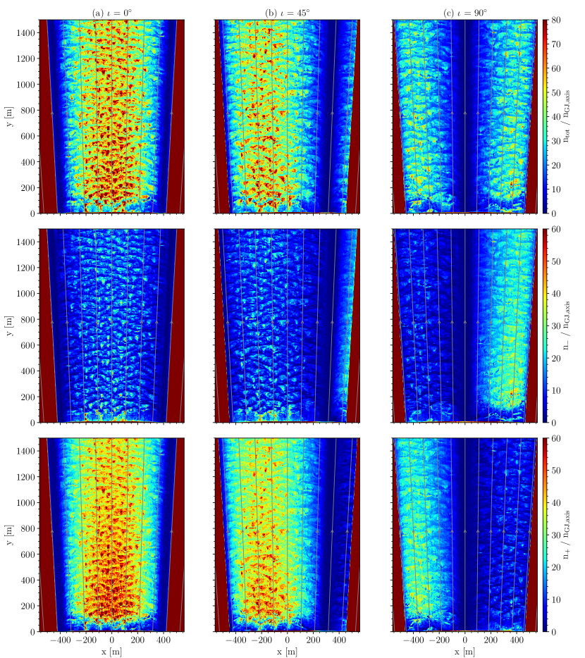
Figure 3: Total (top row), electron (middle row), and positron (bottom row) plasma density at the end of the simulation time normalized to the Goldreich–Julian density, $j_{\mathrm{GJ,axis}}$. The inclination increases from left to right. The magnetic field lines are denoted as grey lines. Animation of the video can be found on Zenodo¹.

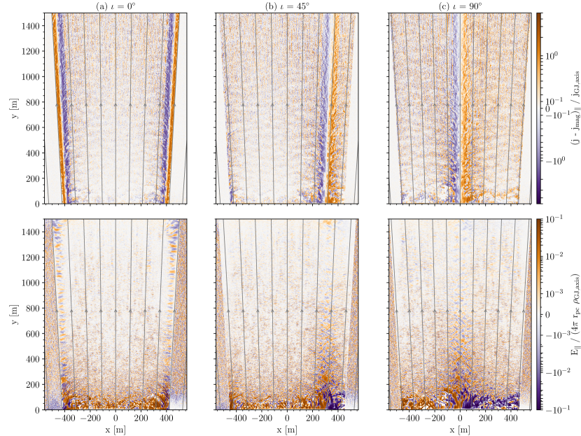
Figure 4: The same as Figure 3 but for parallel electric currents (top row) and parallel electric field (bottom row). The magnetospheric currents are subtracted from the electric currents.

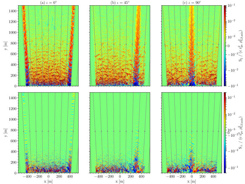
Figure 5: The same as Figure 3 but for the parallel (top row) and perpendicular (bottom row) Poynting flux to the external magnetic field at the end of the simulation time.

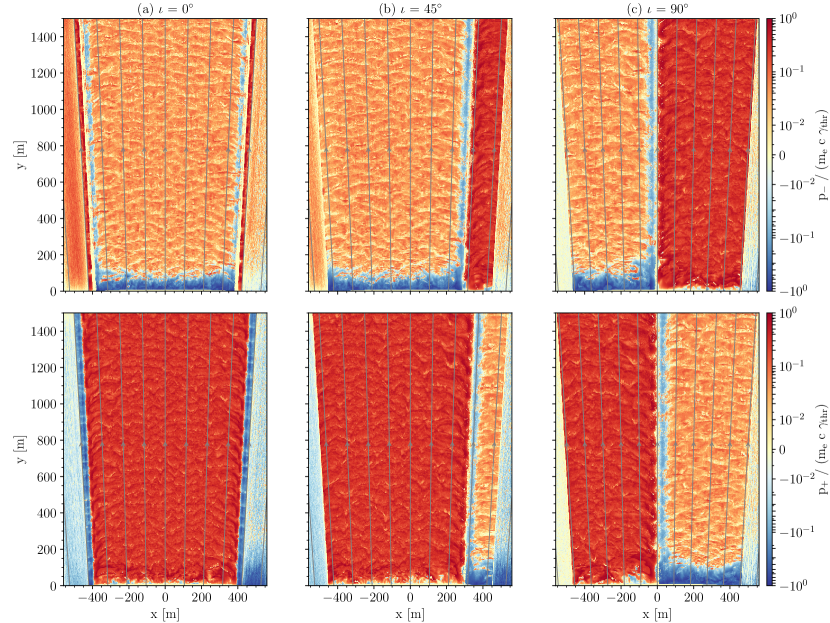
Figure 6: The same as Figure 3 but for the electron (top row) and positron (bottom row) bulk velocities.

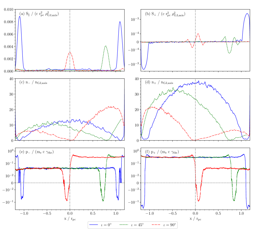
Figure 7: Time-averaged plasma quantities across the polar cap in $x$-axis for $y=11\,000\,\Delta_{\mathrm{x}}=1474$ m. Time average between 130 000 and 150 000 time steps. Top row: Poynting flux parallel and perpendicular to the external magnetic field. Middle row: electron and positron plasma density. Bottom row: momenta of electrons and positrons.

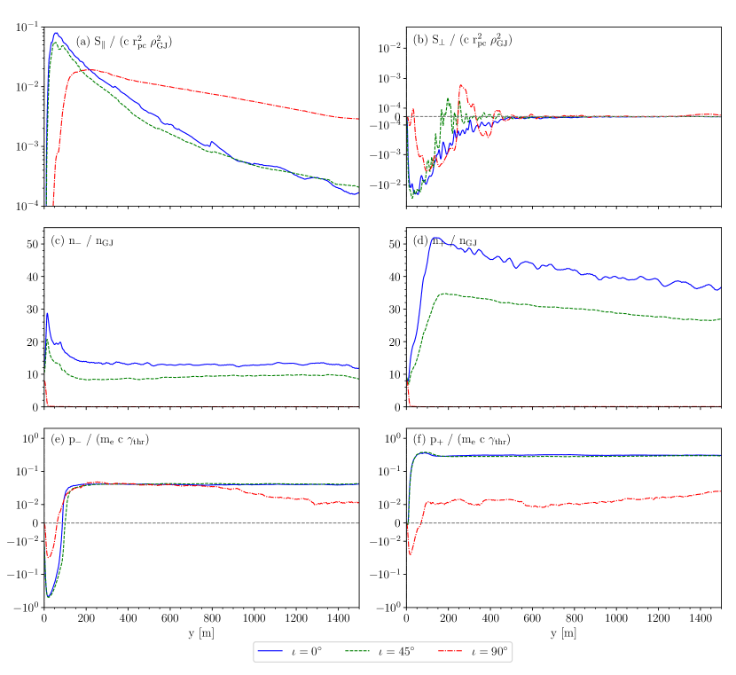
Figure 8: The same as Figure 7 but for a cut along the dipole axis and $x=0$.

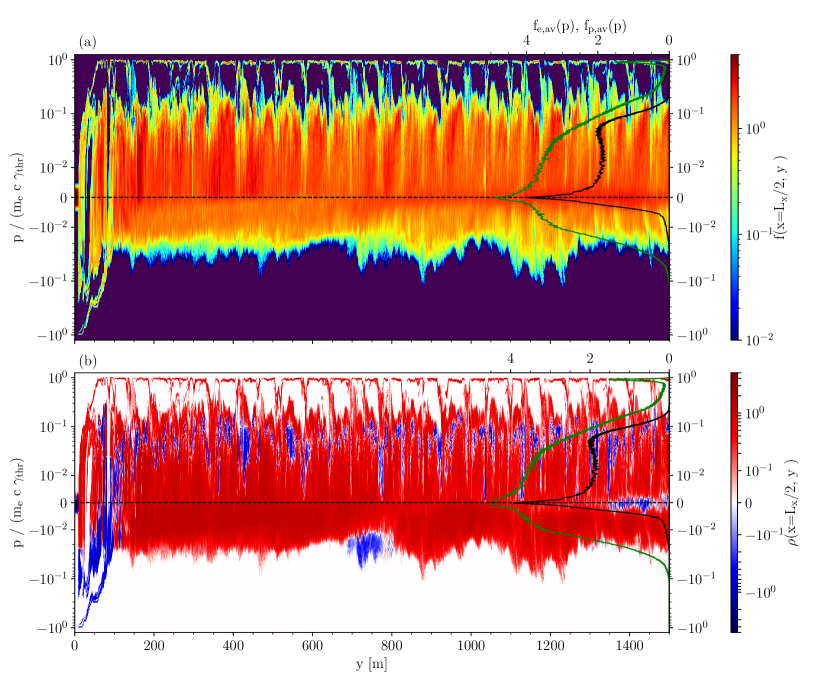
Figure 9: Particle phase space distributions for the pulsar with $\iota=0^{\circ}$ along the magnetic dipole axis at $x=0$ at the end of the simulation time. Black and green lines: Average particle distributions of electrons $f_{\mathrm{e,av}}(p)$ and positrons $f_{\mathrm{p,av}}(p)$, respectively, in a distance range $y=800$–1400 m. Top: Particle number density. Bottom: Charge density. The white regions have zero charge density distribution (if $f(r,p)>0$) or there are no particles (if $f(r,p)=0$).

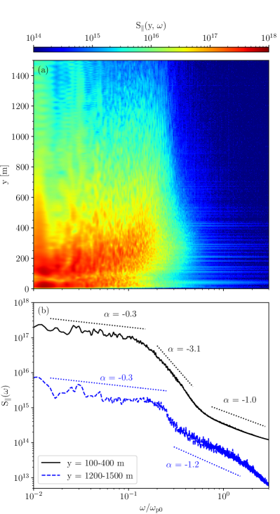
Figure 10: Spectrum of the parallel Poynting flux for the pulsar with $\iota=90^{\circ}$ at the dipole axis between time steps 130 000–150 000. Top: spectrum as a function of the pulsar distance. Bottom: Average spectrum for two ranges of distances from the star surface. Power-law (dotted) lines and indices are denoted.

After the simulation starts, the polar cap goes through two distinct evolutionary phases before it settles into a quasi-periodic discharge formation in the gap close to the star surface. The described simulation setup is designed to go through these stages effectively and relatively fast. The notation of scaled quantities by primes is omitted in this section — all quantities associated with the skin depth, plasma density, and electromagnetic fields are scaled. The time and space quantities remain the same, i.e., $t=t^{\prime}$, $x=x^{\prime}$, and $y=y^{\prime}$.

3.1 Initial convergence of polar cap evolution

In the first phase, the parallel electric fields grow because of the magnetospheric currents described by Equation 3. For a video, please see Zenodo. After the simulation start, the plasma particles are accelerated by the electric field until they reach the threshold Lorentz factor and begin to produce pairs. It takes several hundred time steps for the first particles to reach the threshold Lorentz factor. New pairs are created until the plasma currents sustain the magnetospheric currents in Equation 3, and the electric intensities decrease far enough so that particles cease being accelerated. The polar cap regions where the magnetospheric currents are close to zero are not, or only slightly, populated by secondary particles. When the pair production decreases and approaches zero at the end of this phase, the plasma density is typically much larger than the Goldreich–Julian plasma density and the plasma particles are relatively smoothly distributed in space.

Perpendicular electric fields are mainly generated when secondary particles are being produced. The secondary particles are generated in pairs, leading to an initial local charge neutrality; however, the pairs will be quickly separated when strong electric fields are present. The randomly distributed formation of the charged particles across the magnetic field leads to the formation of electric fields with perpendicular and parallel components to the magnetic field lines. The perpendicular fields do not interact with the particles via wave–particle interactions because the particles cannot move across the field lines. The waves associated with perpendicular electric fields propagate at velocities close to the speed of light and mostly along the magnetic fields. They are eventually absorbed on the star surface or leave the open magnetic field region. At the end of the first phase, the polar cap is filled with plasma that can sustain the magnetospheric currents, the electric fields are close to zero, and the pair production has ceased.

In the second phase, the plasma flows out of the simulation domain until there is not enough plasma to carry the magnetospheric currents. When the plasma cannot sustain the full magnetospheric currents anymore, the electric fields begin to grow again, and new secondary particles are generated in two transient gap regions of open magnetic field lines close to the simulation boundaries — close to the star surface and at the upper boundary that is opposite to the surface.

The plasma density is small in these transient gaps, and the parallel electric fields grow fast. The pair production restarts, and quasi-periodic cascades of plasma bunch generation establish themselves. The resulting bunches have relatively regular shapes in space, that being caused by the smooth profile of magnetospheric currents and plasma density, that are the result of the symmetrical plasma outflow. The bunches flow away from the gap regions and move inward from the boundaries of the simulation domain, their shapes changing as they propagate through the simulation domain. The discharges are however suppressed when the first generation bunches reach the opposite gaps in the simulation.

The perpendicular electric fields have higher amplitudes in the second stage than in the first because the plasma particles are organized into larger density structures associated with local non-zero charge densities. The perpendicular electric fields reach the same intensity as the parallel electric fields at the bunch edges, but the bunch production at the upper boundary opposite to the surface decreases. A Poynting flux associated with oscillating electric and magnetic field components, $\boldsymbol{S}=\frac{c}{4\pi}\boldsymbol{E}\times\delta\boldsymbol{B}$, is produced at the bunch edges. Please, note that the time-averaged electric field is zero, and the only electric fields present are the perturbed ones, $\boldsymbol{E}=\delta\boldsymbol{E}$, where $\delta\boldsymbol{E}$ is the perturbation, while the magnetic field time-average is the magnetic dipole $\boldsymbol{B_{\mathrm{dip}}}$ with perturbation $\delta\boldsymbol{B}\neq\boldsymbol{B}\equiv\boldsymbol{B}_{\mathrm{dip}}+\delta\boldsymbol{B}$.

The system is finally quasi-stable after these two phases, and only an oscillating gap close to the star surface remains as a source of electron–positron pairs. This quasi-periodic state of the polar cap is reached after approximately $\approx 110\,000$ time steps, $\sim 4.1L_{\mathrm{y}}/c$. We continue the simulation for an additional 40 000 time steps, $1.5L_{\mathrm{y}}/c$, in order to reach the final quasi-equilibrium state. Figures 3–6 show snapshots of plasma parameters in the simulation domain at the end of the simulation.

3.2 Plasma properties in quasi-periodic state

Figures 3–6 present the final plasma properties in the polar cap for all three inclination angles at the end of the simulation. The figures are overlaid by the dipole magnetic field lines. Because weak numerical fluctuations keep being formed close to the upper boundary $y=L_{\mathrm{y}}$, we omit that part of the simulation domain from the figures.

Figure 3 shows the total, electron, and positron plasma density normalized to the Goldreich–Julian number density at the dipole axis on the star surface for an aligned pulsar, $n_{\mathrm{GJ,axis}}$. The positron density is larger than the electron density almost everywhere for all three dipole inclinations, in particular on the open field lines and in all regions of negative magnetospheric current where the ratio $j_{\mathrm{mag}}/j_{\mathrm{GJ,axis}}$ is positive. The electron densities increase, and the corresponding positron densities decrease only in the gap close to the star surface $y=30-150$ m; please, see the electric fields and Poynting fluxes below for more details about the gap localization. Because the magnetospheric current switches polarity across the polar cap (Figure 2), the density ratio of electrons and positrons also changes. Those open field lines where the magnetospheric current density goes to zero are filled with significantly fewer particles, thereby forming density cavities. The plasma density in the closed field lines turns out to be much larger than the Goldreich–Julian current density.

Electric current densities and electric fields parallel to the magnetic field lines are shown in Figure 4 with the current density being normalized to the Goldreich–Julian current density, $j_{\mathrm{GJ,axis}}(\boldsymbol{B}_{\mathrm{dip,axis}})$. The electric field is normalized by the radius of the polar cap, $r_{\mathrm{pc}}$, and the Goldreich–Julian charge density for an aligned pulsar at the dipole axis on star surface, $\rho_{\mathrm{GJ,axis}}(\boldsymbol{B}_{\mathrm{dip,axis}})$, in order to obtain a dimensionless quantity. The strongest currents and electric fields are formed in the gap regions close to the star surface, with the electric field amplitudes decreasing with increasing distance from the star. The currents and electric fields are however bf not enhanced in regions of low magnetospheric current (Figure 2). This happens as a consequence of too few particles being available to sustain the magnetospheric currents, and also insufficient numbers of particles that can be accelerated to produce enough pairs for quenching the electric fields.

The amplitude of the parallel electric field $E_{||}$ reaches values about $\approx 6.6\times 10^{10}\,\mathrm{V}\,\mathrm{m}^{-1}$ for all three inclination angles. Accelerating a particle at rest in the gap to the kinetic energy corresponding to $\gamma_{\mathrm{thr}}$ ($\approx$$10^{13}$ eV) requires a distance of $150$ m in this field, assuming that the electric field is constant in time and space during the acceleration. This acceleration distance is consistent with the above estimated size of the gap.

Figure 5 shows Poynting flux parallel and perpendicular to the external magnetic field lines. The Poynting flux is normalized to the radius of the polar cap, $r_{\mathrm{pc}}$, and the Goldreich–Julian charge density, $\rho_{\mathrm{GJ,axis}}(\boldsymbol{B}_{\mathrm{dip,axis}})$. The dominant electric field component of the parallel flux is perpendicular to the external magnetic field and lies on the $\boldsymbol{x}-\boldsymbol{y}$ plane. For the perpendicular flux, the dominant component is the electric field parallel to the external magnetic field. The dominant magnetic field components of the flux are associated with these electric fields, i.e., perpendicular to both the corresponding electric field vector and the Poynting flux vector. Hence, the Poynting flux is polarized in the simulation plane.

The parallel Poynting flux is larger than the perpendicular one as soon as one leaves the gap region. The parallel flux is the largest in open field lines with low magnetospheric currents, where the plasma is not dense enough to absorb the flux. Channels form in the regions of low magnetospheric currents, allowing the Poynting flux to be transported away from the star. In contrast to that, the Poynting flux decreases significantly with the distance from the star in those open field lines with higher magnetospheric current .

The bulk momenta of electrons and positrons are shown in Figure 6. The bulk momenta are calculated as the mean momentum per particle of a given species averaged over the macro-particle weighting function. The momenta are normalized to the electron mass, $m_{\mathrm{e}}$, light speed, $c$, and threshold Lorentz factor, $\gamma_{\mathrm{thr}}$. The positrons have larger bulk momenta than electrons in the regions of positive current ratio $j_{\mathrm{mag}}/j_{\mathrm{GJ,axis}}$. For the opposite sign of the magnetospheric current, the bulk momenta of electrons are larger than for positrons. Both particle species have positive velocities at distances larger than $\sim$$r_{\mathrm{gap}}$$\sim$150 m.

3.3 Time-averaged profiles across and along the polar cap

Figures 7 and 8 show time-averaged profiles of the Poynting flux, plasma density, and particle momenta across the open magnetic field lines and along the dipole axis ($x=0$), respectively. The quantities are normalized the same way as in Figures 3, 5, and 6. The profiles are obtained as time-averaged profiles from the last 20 000 times steps. This time interval is estimated to be long enough to cover the generation of $\approx 6-12$ consecutive bunches. The data were retrieved from line cuts across the polar cap and along the dipole axis for every 20-th time step with a width of one grid cell.

The profiles across the simulation domain in $y=11\,000\,\Delta_{\mathrm{x}}=1474$ m and along the $x$-axis are presented in Figure 7. The Poynting fluxes are enhanced in regions with low magnetospheric currents (Figure 2). That is, the highest fluxes shift from the polar cap edges for $\iota=0^{\circ}$ to the dipole axes for $\iota=90^{\circ}$. The ratio between electron and positron densities depends on the magnetospheric current. The densities have a maximum inside the polar cap and a decrease towards the last open magnetic field lines. For $\iota=90^{\circ}$, the profiles are symmetrical between left–right side of the figures ($x<0$ and $x>0$, respectively) for parallel Poynting flux and plasma densities. Also, the profile is antisymmetrical for perpendicular Poynting flux. The profiles in the closed field lines are not drawn in Figure 7.

In Figure 8, the average Poynting flux amplitude increases with the distance close to the star, but beyond the gap, the flux decreases. The average plasma density is very close to zero because there is only a limited number of particles along the dipole axis for $\iota=90^{\circ}$. For other inclinations, the electron density decreases with the distance from the star surface up to a distance of $\sim 200$ m, remaining approximately constant at larger distances. The positron density increases in the gap region with the distance up to $\sim 200$ m and further away, it decreases with distance. The bulk velocities of both species increase with the distance in the gap region but remain approximately constant further out.

3.4 Particle phase space and wave spectrum along the dipole axis

Figure 9 shows the phase space distribution of the particle number and charge densities along the dipole axis for $\iota=0^{\circ}$ in a selected region of a width of $4d_{\mathrm{e}}$. The plots are overlaid by electron (black line) and positron (green line) distribution functions $f_{\mathrm{e,av}}(p)$ and $f_{\mathrm{p,av}}(p)$ averaged in a distance range $y=800$–1400 m. The distributions are normalized as

$$\int_{-1}^{1}\frac{(f_{\mathrm{e,av}}+f_{\mathrm{p,av}})}{m_{\mathrm{e}}c\gamma_{\mathrm{thr}}}d\mathrm{p}=1.$$

Primary particles, their Lorentz factors being close to the threshold decay Lorentz factor, are in evidence in the upper parts of both subfigures where the momenta are $p/(m_{\mathrm{e}}c\gamma_{\mathrm{thr}})\sim 1$ The particles reach the $p/(m_{\mathrm{e}}c\gamma_{\mathrm{thr}})=1$ at distances of 100–200 m from the star in the gap region. The phase space distributions show regular phase space holes around $p/(m_{\mathrm{e}}c\gamma_{\mathrm{thr}})\approx 0.2-0.8$ and distances $>50$ m. The holes are created for both the primary and secondary particle distributions and are associated with the discharge modulation of the primary particles occurring in the polar cap. The plasma has a relativistically broad distribution ranging from negative values of $p/(m_{\mathrm{e}}c\gamma_{\mathrm{thr}})\approx-0.05$ to positive once $p/(m_{\mathrm{e}}c\gamma_{\mathrm{thr}})\approx 0.2$ in the broad band where the momenta are below the maximum for the holes. Most of the charge density phase space is dominated by positive charges; however, there are regions of negative density inside the plasma bunches. Some particles flow back on the star at $y=0-100$ m and $p/(m_{\mathrm{e}}c\gamma_{\mathrm{thr}})\approx-1$ to $-0.1$, being composed mostly of electrons (the blue structures). This electron flow also reaches the threshold momentum for negative momenta and may produce pairs close to the star surface.

Figure 10 shows the spectrum of the outgoing Poynting flux at the dipole axis of one grid cell width for the Poynting flux channel for the pulsar with inclination $\iota=90^{\circ}$. The spectrum is averaged over time steps 130 000–150 000 ($\approx$$26.1-30.2\,\mu$s). Only positive values were chosen for the calculation of the outgoing parallel Poynting flux — negative values of the Poynting flux occur approximately in the gap region. The frequency is normalized to the initial, non-relativistically calculated plasma frequency, $\omega_{\mathrm{p0}}$. Most of the spectral power is emitted below $\omega_{\mathrm{p0}}$ mainly because the plasma is relativistically hot and the local plasma frequency decreases as $\sim\langle 1/\gamma^{3}\rangle$. All waves have higher intensities up to $y<400$ m than at larger distances where they are partially absorbed. Most energy is absorbed in the region $\lesssim 0.2\omega_{\mathrm{p0}}$. For the distance $y=100$–400 m, the spectrum has three power-law parts with indices $-0.3$, $-3.1$, and $-1.0$, while for distance $y=1200$–1400 m, the spectrum has indices $-0.3$ and $-1.2$ with a small but steeper transition region between them at $\omega/\omega_{\mathrm{p}}\approx 0.2-0.3$. We also found that most of the waves follow the vacuum dispersion relation of the electromagnetic waves $\omega\approx ck$ for almost all frequencies.

4 Discussion

The polar caps of neutron star magnetospheres produce pair cascades and are sources of coherent radio emissions, ultrarelativistic particles, and plasma outflows. We carried out 2D kinetic particle-in-cell simulations of the polar cap close to the star surface where the polar gap is located. We studied how the inclination angle of the magnetic dipole influences the discharge behavior, bunch generation, and Poynting flux transport.

The main driving mechanisms of the polar cap pair cascades are the magnetospheric currents and their polarity switch across the polar cap. We found that the Poynting flux is effectively transported away from the gap and through the magnetosphere in regions of open magnetic field lines where the magnetospheric currents are close to zero, denoted as the Poynting flux channels. The plasma has only a low density in these channels because of the weak or lacking secondary plasma generation. The Poynting flux channel locations depend on the inclination angle of the dipole field. For an aligned pulsar, there are two channels at polar cap edges close to the closed field lines. For increasing inclination angle, the channels with larger latitudes diminish, and the second channel shifts toward the dipole axis and reaches it for an orthogonal pulsar.

The width of the transport channel across the magnetic field lines is determined by the boundaries of the regions where the plasma can sustain the magnetospheric currents without significant pair production. In the simulation, we impose the condition for a minimal plasma density at the boundary that corresponds to the plasma frequency $\omega_{\mathrm{p0}}$, in our simulations represented by 2 PPC of the boundary condition. However, a choice of another minimal density, e.g., by the Goldreich–Julian current density (Beloborodov, 2008), could change the channel width.

4.1 Poynting flux properties

Because the plasma density is low in the Poynting flux channel, the electromagnetic wave frequencies are above the relativistically corrected plasma frequency, i.e., $\sim(10^{-4}-10^{-3})\omega_{\mathrm{p0}}\ll\omega_{\mathrm{p0}}$ (Figure 10), and the absorption in the channel is low. The Poynting flux enters the channel in the gap region where it is very high, propagating from there out in various directions. The parallel component of the flux dominates the perpendicular component by a few orders of magnitude after a certain propagation distance along the channel. The perpendicular component is quickly absorbed by its reflections on the channel boundaries that have higher plasma densities than the channel. Specifically, a part of the electric field component parallel to the external magnetic field can be absorbed because the plasma can partially screen out that electric field. We also found that the electric and magnetic waves of the Poynting flux follow the electromagnetic wave dispersion relation in vacuum $\omega=ck$, and the Poynting flux can, therefore, be interpreted as being composed from electromagnetic waves. The spectra of escaping waves can be described by broken power laws, having a relatively flat low frequency region and a steeper high frequency part, with respective indices of $-0.3$ and $-1.2$. It is conceivable that the Poynting flux in the channels and the flux associated with the bunches in high density region can propagate out and leave the magnetosphere as electromagnetic waves that would then be observed as pulsar radio emission.

In the regions of high magnetospheric currents, irregular pair plasma bunches and clouds of particles are formed in the gap close to the star surface of a thickness of $\sim 150$ m. Though the plasma density significantly varies in the bunch, the bunch shape only weakly changes during its propagation along the magnetic field lines. The Poynting flux is absorbed in these regions by the plasma, in contrast with the low density channels, and the flux decreases with the distance from the star. We have tested the Poynting flux decrease in intensity for various simulation setups. The decrease is independent of the simulation grid cell size and PPC as long as these parameters allow sufficient resolution of the polar gap and the released bunches.

Assuming that the Poynting flux channel also exists at a larger distance from the star than the length of the simulation domain, the Poynting flux can be captured in the channel until it reaches a distance at which the wave frequencies exceed the plasma frequency outside the channel. Thus, the higher frequency waves could escape the channel earlier than the low frequency ones because their frequencies earlier exceed the plasma frequency of the surrounding plasma. For an observation at an arbitrary radio frequency, the channel could serve as a “waveguide” through the magnetosphere into the wave origin — the gap. By observing a low-frequency cut-off in radio frequencies, we could estimate the maximal allowed plasma density in the emission region — that is, the plasma frequency and maximal density in the channel.

As the Poynting flux propagates through the channel, it may undergo reflections at the channel boundaries because the refractive index of the plasma increases towards the more dense regions. In addition, only the reflection of the Poynting flux component polarized perpendicular to the channel boundary is expected, similar to the reflection of a light wave in an optical fiber. Thus, we hypothesize that if the Poynting flux escapes the channel as electromagnetic waves, its polarization can follow the channel’s geometric structure. This way, the observed polarization profiles of pulsars could be directly related to the geometrical structure of the Poynting flux channel in the polar cap.

Low density magnetic channels, called flux tubes, similar to those in our simulations have also been found in theoretical papers from solar physics (Wu et al., 2002; Schlickeiser & Skoda, 2010; Treumann & Baumjohann, 2014) and there have also been recent in situ detections (Chen et al., 2023). An electromagnetic wave can propagate inside the flux channel until the surrounding plasma density decreases with the distance from the Sun and the wave frequency exceeds the plasma frequency of the surrounding material.

4.2 Plasma bunch properties

It is however in general not straightforward to determine the typical distance between the bunches that are released from the gap region from our simulations. While the gap in the simulations spreads out up to the distance of $\sim 150$ m from the star surface, similar to Sturrock’s model (Sturrock, 1971), the consecutive bunches are closer together, being separated only by $\sim$50–100 m. The bunches are, moreover, not equidistantly distributed along or across the magnetic field lines. Their distance depends on the strength of the magnetospheric current: typically, the gap size is larger for lower magnetospheric currents and, therefore, larger for lower dipole magnetic fields. Hence, the distance varies with the magnetospheric current profile across the polar cap.

The bunch sizes and distances are also significantly influenced by the values of primary particle Lorentz factors at which they begin to emit $\gamma$-ray photons energetic enough to produce pairs. This relation is however not a simple function of the plasma parameters. A lower number of secondary particles produced from lower $\gamma-$ray emission can lead to a lower secondary plasma density and lower plasma currents and can result in higher electric field intensities. The high-intensity fields may change the typical acceleration distance, gap size, and bunch distances.

4.3 Comparison with previous 2D PIC simulation

There is only one 2D PIC simulation of the polar cap, that resolves realistic sizes of the gap region and the bunches that we could use for comparison with our results (Cruz et al., 2021a). The structure of bunches, their distances, and sizes obtained from our simulations are different from theirs because of differences in the magnetospheric parameters and simulation setup. The pair cascades in our simulations are driven by local magnetospheric currents formed as the result of the curvature of magnetic field lines. The current profile, which is used across and along the polar cap, is a solution of global force-free general-relativistic simulations, and the profile changes with the dipole inclination angle. The simulations by Cruz et al. (2021a) drive the cascade by electric fields present at the star surface and are implemented as the boundary condition for an arbitrary profile across the polar cap. In addition, it is unclear whether the simulations were carried out long enough so that a quasi-steady state can evolve with the cascade.

The distances between bunches are smaller in our simulations because they depend on the strength of magnetospheric currents. We assumed that the magnetospheric currents correspond to a pulsar with $P=0.25$ s and a dipole magnetic field of $10^{12}$ G at the surface.

Another important process that can significantly increase the bunch distances, as showed by Cruz et al. (2021a), is the $\gamma$-ray photon propagation distance before they decay into pairs. We have not included this effect in our simulations. For a more precise consideration of the QED effects of the $\gamma$-ray photon emission and decay, we expect a smoother density profile of the bunches as both the photon emission and pair producing distances will have a distribution of values. The probability distributions of the QED effects are however included in our approach in the form of an appropriate a step function at the threshold Lorentz factor. The maximal Lorentz factor that particles can reach is strongly dependent on the radiative energy losses. It is however uncertain how high the Lorentz factors the primary particles can reach when all types of radiative losses (like curvature, synchrotron, and linear acceleration emission losses) are included.

5 Conclusions

We investigated the pair cascades in the polar cap of neutron stars magnetospheres by particle-in-cell simulations at kinetic scales, aiming to find out how the magnetic dipole inclination impacts the production of plasma bunches and the generation and possible escape of electromagnetic radio waves in the form of Poynting flux. We found that the high intensity Poynting flux generated in the electric gap close to the star surface can be transported in channels of low plasma density through the magnetosphere without significant absorption. The transport channels are located along open magnetic field lines where the magnetospheric currents approach zero (Gralla et al., 2017). Oppositely, outside these channels, for example, at the edges of plasma bunch discharges, the generated Poynting flux decreases quickly with the distance from the star.

It is interesting to note that no conversion process from the kinetic energy of plasma particles to electromagnetic waves is necessary in order to emit a high-intensive radiation field, as the obtained broad spectrum of escaping electromagnetic waves is directly generated by the oscillating electric field gap. This result is fundamentally different from that for most other theoretical mechanisms of pulsar radio emission where high conversion efficiencies of plasma waves to coherent radio emissions are required. (Eilek & Hankins, 2016; Melrose et al., 2020; Philippov & Kramer, 2022). The escaping electromagnetic waves have two power-law regions with indices -0.3 for $\omega/\omega_{\mathrm{p}}\approx 0.01-0.2$ and -1.2 for $\omega/\omega_{\mathrm{p}}\approx 0.3-2$, similar to those observed in pulsars (Bilous et al., 2016).

Our model implies that the pulsar radio beam does not have a symmetrical cone-like structure, but rather the radio waves that propagate from the gap with oscillating electric fields in channels along open magnetic field lines where no pair cascades occur and the plasma density is low. Therefore, the shape of the pulsar radio beam is defined by the shape of magnetic field lines without pair production. The frequently conjectured frequency–to–radius relation of the escaping radiation has no real basis in emission physics and has also been shown to be incompatible with observations by Hassall et al. (2012, 2013).

The detected behavior of the Poynting flux poses the question of whether the Poynting flux outside or inside the Poynting flux channels can reach higher altitudes in the magnetosphere and leave the magnetospheric plasma as electromagnetic radio waves. We hypothesize that the flux in the form of electromagnetic waves can reach higher altitudes and is efficiently captured in the channel as long as the decreasing plasma frequency in the surrounding field lines is higher than the electromagnetic wave frequency. The waves could escape the channel beyond that point. In addition, if the observed radiation of pulsar pulses is transported in such a Poynting channel, the pulse profile and the pulse maxima will be correlated with the Poynting flux channel position and the field lines with very low or zero current. In order to interpret the pulsars with more than two radio peaks, one has to assume more complex structures of the magnetospheric current across the polar cap than those given by a simple magnetic dipole (Lockhart et al., 2019).

Our numerical simulations have been found to be resilient to moderate changes in initial and boundary conditions; these simulations can, therefore, allow more detailed future studies of various aspects of the discharge evolution in the neutron star polar cap, like the star surface heating, high energy emissions, particle acceleration, various additional processes leading to radiative losses, and the quantum-electrodynamic pair creation.