On the sequential convergence of Lloyd’s algorithms

Abstract

Lloyd’s algorithm is an iterative method that solves the quantization problem, i.e. the approximation of a target probability measure by a discrete one, and is particularly used in digital applications.This algorithm can be interpreted as a gradient method on a certain quantization functional which is given by optimal transport. We study the sequential convergence (to a single accumulation point) for two variants of Lloyd’s method: (i) optimal quantization with an arbitrary discrete measure and (ii) uniform quantization with a uniform discrete measure. For both cases, we prove sequential convergence of the iterates under an analiticity assumption on the density of the target measure. This includes for example analytic densities truncated to a compact semi-algebraic set. The argument leverages the log analytic nature of globally subanalytic integrals, the interpretation of Lloyd’s method as a gradient method and the convergence analysis of gradient algorithms under Kurdyka-Lojasiewicz assumptions. As a by-product, we also obtain definability results for more general semi-discrete optimal transport losses such as transport distances with general costs, the max-sliced Wasserstein distance and the entropy regularized optimal transport loss.

1 Introduction

Quantization aims to approximate a target probability measure $\mu$ on $\mathbb{R}^{d}$ by a discrete, finitely supported measure. We consider two quantization settings induced by an optimization problem in Wasserstein distance. First, optimal quantization consists in approximating the target measure $\mu$ with a discrete probability measure supported on $N$ points $y_{1},\ldots,y_{N}\in\mathbb{R}^{d}$ with weights $\pi\in\Delta_{N}$, the $N-1$ dimensional unit simplex, by solving the following optimization problem:

$$\underset{y_{1},\ldots,y_{N}\in\mathbb{R}^{d}}{\min}\ \underset{\pi\in\Delta_{N}}{\min}\qquad W_{2}^{2}\left(\mu,\sum_{i=1}^{N}\pi_{i}\delta_{y_{i}}\right).$$ (1.1)

It is a central problem in signal processing to convert a continuous-time signal into a digital one Graf and Luschgy (2000); Pagès (2015). Second, uniform quantization consists in approximating $\mu$ with a discrete measure, corresponding to constraints on the optimal quantization weights:

$$\underset{y_{1},\ldots,y_{N}\in\mathbb{R}^{d}}{\min}\qquad W_{2}^{2}\left(\mu,\frac{1}{N}\sum_{i=1}^{N}\delta_{y_{i}}\right).$$ (1.2)

In both problem, $W_{2}^{2}$ denotes the squared $2$-Wasserstein distance, the optimal transport distance for the squared Euclidean cost between probability measures (see e.g. Villani (2021, 2008); Santambrogio (2015)). The Wasserstein distance is well suited in this context since it allows to handle the semi-discrete nature of the quantization task. The main question addressed in this work is that of the asymptotic convergence of the well known Lloyd iterative algorithmic method for problems (1.1) and (1.2). Note that both problems are non-convex and iterative solvers typically aim to find a stationary point rather than solve the global problem.

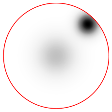
(a)

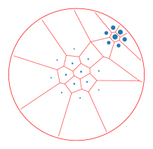
(b)

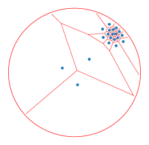
(c)

Figure 1: (Left) Target gaussian mixture $\mu$ with two components truncated on a disk. (Middle) Optimal quantization of $\mu$ with $20$ points (blue) and their corresponding Voronoi cells (in red) after $250$ iterations of Lloyd’s algorithm. (Right) Uniform quantization of $\mu$ with $20$ points (blue) and the corresponding power cells (in red) after $5$ iterations of Lloyd’s algorithm adjusted for uniform quantization. The diameter of a blue dot is proportional to its weight. The algorithms are randomly initialized and run using the PyMongeAmpere library¹.

Lloyd-type algorithms.

In his early paper Lloyd (1982), Lloyd proposes an algorithm to solve the least squares quantization problem in the univariate setting (without mentioning optimal transport at that time). Lloyd defines a quantization scheme using intervals and their centroids and introduces an iterative algorithm consisting in alternating optimization steps on the intervals and on the centroids. The generalization of this method to the multivariate setting involves cendroidal Voronoi cells Du et al. (1999) which can be interpreted as optimal transport maps in the optimal quantization formulation in (1.1). In this setting, Lloyd’s method alternates between evaluation of Voronoi cells (given centroids), and update of centroids (given Voronoi cells).

Lloyd’s method can be extended to the case of uniform quantization in (1.2), for which the Voronoi cells encompass a volume constraint Balzer et al. (2009). We refer to them as power cells. These regions are also associated to optimal transport maps in the uniform quantization problem in (1.2) De Goes et al. (2012), and algorithms have been developed for computing these power cells Kitagawa and Thibert (2019). Both methods, for optimal or uniform quantization, share the same overall “alternating” structure and we will refer to both of them as Lloyd’s method. They are illustrated in Figure 1, generated using the PyMongeAmpere library. A precise description of Lloyd’s method for optimal and uniform quantization is given in Section 2 with Algorithm 1 and 2.

We address the question of sequential convergence of the iterates produced by Lloyd’s method for solving (1.1) and (1.2). More precisely, we consider the asymptotic stabilization of the support points $y_{1},\ldots,y_{N}$ of the Dirac masses to a critical point of the quantization functional. This question was already considered in previous literature. For optimal quantization, the first analyses were proposed for the univariate case Wu (1992); Kieffer (1982) with special cases such as the strict log-concavity of the target measure density Fleischer (1964); Du et al. (1999). In the multivariate setting, it is known that accumulation points of Lloyd’s iteration are critical points of the loss in (1.1) Du et al. (2006); Emelianenko et al. (2008); Pagès and Yu (2016). In particular if such critical points are isolated, an assumption very difficult to check in practice, then the algorithm converges. For uniform quantization, similar results exist. It was shown for example that accumulation points of Lloyd’s method are critical points of the functional in (1.2), leaving the convergence of the whole sequence open Mérigot et al. (2021).

In this work, we prove convergence of the sequence generated by both Lloyd’s methods under an explicit definability assumption on the density of the target measure $\mu$. Note that, we do not consider convergence toward the global minimizer of the quantization functional and limit ourselves to critical points.

Convergence of gradient sequences and rigidity of semi-discrete optimal transport losses.

Both results rely on the interpretation of Lloyd’s methods as gradient schemes for problems (1.1) and (1.2) Du et al. (1999); Mérigot et al. (2021). In a non-convex setting, the iterates of gradient sequences converge under Lojasiewicz inequality, for example if the underlying loss function is analytic Absil et al. (2005). Kurdyka proposed a generalization of Lojasiewicz’s property that holds true for all functions that are definable in an o-minimal structure Kurdyka (1998), which we refer to as the Kurdyka-Lojasiewicz (KL) inequality. Definable functions represent a broad and versatile class of functions and covers many applications. For example this class is closed under composition, partial minimization / maximization, etc. Convergence of first order methods under KL assumptions have now become standard in non-convex optimization, see for example Attouch et al. (2013); Bolte et al. (2014) and references therein. This is the main path that we follow.

Applying Kurdyka’s result to (1.1) and (1.2) requires to justify that these functions are definable in some o-minimal structure. This is far from direct as the description of these functionals involve integrals and o-minimal structures are not stable under integration in general. This is one of the great challenges of this field, several partial answers are known, one of them allowing to treat the definability of globally subanalytic integrals Lion and Rolin (1998); Comte et al. (2000); Cluckers and Miller (2011) which have a log-analytic nature. This is the crucial step behind our convergence results, an observation already made in Bolte et al. (2023) in a stochastic optimization context. We work under the assumption that the compactly supported target measure has a globally subanalytic density (see Assumption 1). This allows to justify the resulting log analytic nature of the losses in (1.1) and (1.2). Convergence then follows using the well known connection between Lloyd’s method and the gradient algorithm and its convergence analysis under KL assumptions.

The proposed analysis opens the question of definability of semi-discrete optimal transport losses beyond the $2$-Wasserstein distance in (1.1) and (1.2). We justify the definable nature of several such losses involving general optimal transport costs, sliced Wasserstein distance Rabin et al. (2012); Bonneel et al. (2015); Bobkov and Ledoux (2019), the max-sliced Wasserstein distance Kolouri et al. (2019); Deshpande et al. (2019), and entropy regularized optimal transport Cuturi (2013). These results are of independent interest, and may be relevant to study numerical applications of optimal transport.

Organization of the paper and notations.

We start with a description of Lloyd’s methods and state our main results in Section 2. The central convergence arguments based on KL inequality are described in Section 3, and the definability of the underlying losses is described in Section 4. Extension to broader optimal transport losses is given in Section 5.

Regarding technical elements discussed in the introduction, we recall the definition of KL inequality and the main result of Kurdyka in Section 3.1, while the necessary background on o-minimal structures and globally subanalytic sets is given in Section 4. Furthermore, the precise definition of the $W_{2}$ distance in the semi-discrete setting of (1.1) and (1.2) is postponed to Section 5.1.

The Euclidean norm and the dot product in $\mathbb{R}^{d}$ are denoted $\|\cdot\|$ and $\langle\cdot,\cdot\rangle$. We define respectively the open and closed $d$-dimensional Euclidean ball centered in $x$ with radius $r$ as $B_{d}(x,r)$ and $\overline{B_{d}(x,r)}$.

2 Main results

We use the notation $Y\in(\mathbb{R}^{d})^{N}$ to denote $N$ points $y_{1},\ldots,y_{N}$ in $\mathbb{R}^{d}$ which are candidate support points for quantization. This section contains our main results regarding the sequential convergence of Lloyd’s algorithms for optimal and uniform quantization.

2.1 Assumptions on the target measure

We will consider the following assumptions on the target measure $\mu$ and its density probability function $f$.

Assumption 1.

$\mu$ is a probability measure on $\mathbb{R}^{d}$, with compact support, absolutely continuous with respect to Lebesgue measure, with globally subanalytic density $f$.

Absolute continuity and compacity ensure that Lloyd’s iterations are well defined, see for example (Emelianenko et al., 2008, Assumption 3.1). The global subanaliticity assumption is a rigidity assumption which will allow to invoke KL inequality for our convergence analysis. The precise definition of global subanaliticity is given in Section 4.1. This is a very versatile notion for which we provide a few examples below.

Example 2.1.

The following are globally subanalytic density functions:

• The uniform density on a compact basic semi-algebraic set, of the form $S=\{x,\,P_{i}(x)\geq 0,i=1,\ldots,m\}\subset\mathbb{R}^{d}$, for some $m\in\mathbb{N}$, where $P_{i}\colon\mathbb{R}^{d}\to\mathbb{R}$ are polynomials.

• Densities of the form $x\mapsto f(x)\mathbbm{1}_{S}(x)$ where $S$ is a compact semi-algebraic set (as above) and $f\colon U\to\mathbb{R}$ is an analytic function on an open domain $U\supset S$ (Lemma 4.6). These include truncated Gaussians for example.

• Semi-algebraic densities including integrable rational functions and their restrictions to compact sets.

• Any finite mixture of the above density examples. This allows to consider nonsmooth and possibly discontinuous densities.

• For instance, any normalized image considered as a piecewise constant probability density on the plane is globally subanalytic.

Remark 2.2.

Under Assumption 1, the density $f$ is strictly positive on a full measure open dense set in $\operatorname{Supp}\,\mu$, the support of the measure $\mu$. Indeed the set $\{x,\,f(x)>0\}$ is globally subanalytic and can be partitioned into a finite number of embedded submanifolds in $\mathbb{R}^{d}$ (Dries and Miller, 1996, 4.8). It is enough to keep those of dimension $d$ only since those of dimension at most $d-1$ have zero Lebesgue measure. We deduce that $S=\{x,\,f(x)>0\}$ is non-empty, globally subanalytic and open, we have $\operatorname{Supp}\,\mu=\mathrm{cl}_{\mathbb{R}^{d}}S$ and $\mathrm{dim}(\operatorname{Supp}\,\mu\setminus S)<d$, using (Dries and Miller, 1996, 4.7), which is the claimed statement.

2.2 Optimal Quantization

In addition to the main hypothesis above, the target measure is assumed to have convex support throughout this section.

Assumption 2.

$\mu$ is a probability measure as in Assumption 1, with convex support.

Partial minimization of the objective function in (1.1) with respect to the weights $\pi$ leads to the optimal quantization functional $G_{N}\colon(\mathbb{R}^{d})^{N}\to\mathbb{R}$, see e.g. Graf and Luschgy (2000),

$$G_{N}(Y)\quad=\quad\underset{\pi\in\Delta_{N}}{\min}\quad\frac{1}{2}W_{2}^{2}\left(\mu,\sum_{i=1}^{N}\pi_{i}\delta_{y_{i}}\right)\quad=\quad\frac{1}{2}\int\min_{i=1,\ldots,N}\|x-y_{i}\|^{2}f(x)dx,$$ (2.1)

where we recall that $f$ stands for the density of $\mu$. Problem (1.1) therefore amounts to minimize the objective $G_{N}$. This functional is tightly connected to the so-called Voronoi cells $(V_{i}(Y))_{i=1,\ldots,N}$ associated to the support points $Y=(y_{i})_{i=1}^{N}\in(\mathbb{R}^{d})^{N}$ (Du et al., 1999, Proposition 3.1), and given for $i=1,\ldots,N$ by

$$V_{i}(Y)=\left\{x\in\mathbb{R}^{d}\>|\>\forall j=1,\ldots,N\>:\>\|x-y_{i}\|^{2}<\|x-y_{j}\|^{2}\right\}.$$ (2.2)

The Voronoi cells in (2.2) are open and disjoint, they are all non-empty as long as $Y$ does not belong to the generalized diagonal defined by

$$D_{N} =\{Y\in(\mathbb{R}^{d})^{N}\>|\>\exists i\neq j:y_{i}=y_{j}\}.$$ (2.3)

Therefore, for any $Y\not\in D_{N}$, the optimal quantization functional in (2.1) takes the form

$$G_{N}(Y)\quad=\quad\frac{1}{2}\sum_{i=1}^{N}\int_{V_{i}(Y)}\|x-y_{i}\|^{2}f(x)dx.$$ (2.4)

Note that a local minimizer to (1.1) on $\operatorname{Supp}\mu$ does not lie in $D_{N}$ (Du et al., 1999, Proposition 3.5). Lloyd’s algorithm for computing optimal quantizers is then defined by fixed point iterations of the Voronoi barycentric mapping $T_{N}\colon\operatorname{Supp}\mu\setminus D_{N}\to\operatorname{Supp}\mu\setminus D_{N}$ defined by

$$T_{N}(Y)=\left(\frac{\int_{V_{i}(Y)}xd\mu(x)}{\mu(V_{i}(Y))}\right)_{i=1,\ldots,N},$$ (2.5)

Then the map $T_{N}$ is indeed well defined on $\operatorname{Supp}\mu\setminus D_{N}$ since, for distinct centroids in $\operatorname{Supp}\mu$, the Voronoi cells in (2.2) are non-empty and have non-zero $\mu$ measure. Furthermore $T_{N}$ takes values in $\operatorname{Supp}\mu\setminus D_{N}$ as the centroids remain distinct since the Voronoi cells are disjoint, and they belong to the support of $\mu$ since it is convex by Assumption 2. This is summarized in Algorithm 1 and we prove in Section 3.2 the following theorem regarding convergence of the iterates.

Theorem 2.3.

Let $\mu$ be as in Assumption 2, then the iterates of Lloyd’s algorithm for optimal quantization in Algorithm 1 converge to a critical point of $G_{N}$ in (2.1).

  Input: $\mu$ absolutely continuous probability measure on $\mathbb{R}^{d}$ with convex compact support, $Y_{0}\in\operatorname{Supp}\mu\setminus D_{N}$ as in (2.3).

  for $n\in\mathbb{N}$ do

     $Y_{n+1}=T_{N}(Y_{n})$ where $T_{N}$ is the Voronoi barycentric mapping in (2.5).

Algorithm 1 Lloyd’s algorithm for optimal quantization

2.3 Uniform Quantization

The objective in (1.2) is called the uniform quantization functional $F_{N}\colon(\mathbb{R}^{d})^{N}\to\mathbb{R}$, and is defined as follows

$$F_{N}(Y)\quad=\quad\frac{1}{2}W_{2}^{2}\left(\mu,\frac{1}{N}\sum_{i=1}^{N}\delta_{y_{i}}\right).$$ (2.6)

The uniform quantization problem consists in finding minimizers of $F_{N}$. Similar to optimal quantization, the functional can be explicitly described by power cells (also called Laguerre cells Mérigot et al. (2021)). These generalize Voronoi cells and characterize the optimal transport plan in $W_{2}$ between the target measure and the discrete measure (see also (5.2)). If $Y$ is not in the generalized diagonal $D_{N}$, then $F_{N}$ in (2.6) can be written with the Kantorovich dual formulation introduced as follows for $w\in\mathbb{R}^{N}$ (see for example (Villani, 2008, Theorem 5.9) and (Mérigot et al., 2021, Section 2) for details on the uniform quantization setting)

$$\begin{split}\Phi(Y,w)&:=\frac{1}{2}\left\{\int_{\mathbb{R}^{d}}{\left(\min_{i=1,\ldots,N}\|x-y_{i}\|^{2}-w_{i}\right)f(x)dx}+\frac{1}{N}\sum_{i=1}^{N}{w_{i}}\right\}\\ &=\frac{1}{2}\left\{\sum_{i=1}^{N}\int_{\operatorname{Pow}_{i}(Y,w)}\left(\|x-y_{i}\|^{2}-w_{i}\right)f(x)dx+\frac{1}{N}\sum_{i=1}^{N}{w_{i}}\right\}\end{split}$$ (2.7)

where the power cells $\operatorname{Pow}_{i}(Y,w)$ are defined for $i=1,\ldots,N$ as

$$\operatorname{Pow}_{i}(Y,w)=\{x\in\mathbb{R}^{d}\>|\>\forall j=1,\ldots,N\>:\>\|x-y_{i}\|^{2}-w_{i}\leq\|x-y_{j}\|^{2}-w_{j}\}.$$ (2.8)

Kantorovich’s duality states that for any $Y\not\in D_{N}$, the uniform quantization functional in (2.6) is given by

$$F_{N}(Y)=\max_{w\in\mathbb{R}^{N}}\ \Phi(Y,w).$$ (2.9)

It can be shown (see Remark 3.8) that the maximum in (2.9) is attained and unique up to the addition of a constant. Therefore, it defines a unique set of power cells (2.8), and additionally the $\mu$ measure of each power cell is $\frac{1}{N}$.

We introduce $B_{N}\colon(\mathbb{R}^{d})^{N}\setminus D_{N}\to(\mathbb{R}^{d})^{N}\setminus D_{N}$ the Laguerre barycentric application defined by

$$B_{N}(Y)=\left(N\int_{\operatorname{Pow}_{i}(Y,\phi(Y))}xd\mu(x)dx\right)_{i=1,\ldots,N}$$ (2.10)

where $\phi(Y)$ denotes an element of ${\operatorname{argmax}}_{w\in\mathbb{R}^{N}}\>\Phi(Y,w)$ in (2.7). Note that the Laguerre cells are disjoint and non-empty outside of the generalized diagonal $D_{N}$ so that $B_{N}$ indeed has values in $(\mathbb{R}^{d})^{N}\setminus D_{N}$. Lloyd’s algorithm consists in fixed point iterations of the map $B_{N}$ as summarized in Algorithm 2. Our main result regarding this algorithm is the following, whose proof is postponed to Section 3.3.

Theorem 2.4.

Let $\mu$ be as in Assumption 1, then the iterates of Lloyd’s algorithm for uniform quantization in Algorithm 2 converge to a critical point of $F_{N}$ in (2.6).

  Input: $\mu$ absolutely continuous probability measure on $\mathbb{R}^{d}$ with compact support,

$Y_{0}\in(\mathbb{R}^{d})^{N}\setminus D_{N}$ as in (2.3).

  for $n\in\mathbb{N}$ do

     $Y_{n+1}=B_{N}(Y_{n})$ where $B_{N}$ is the Laguerre barycentric mapping in (2.10).

Algorithm 2 Lloyd’s algorithm for uniform quantization

Remark 2.5.

Contrary to optimal quantization, the convexity of the support is not required here for the algorithm to be well defined, by construction of the power cells at optimality in (2.9). Additionally, the identity in (2.9) only holds if $Y\not\in D_{N}$. It is nonetheless possible to extend it to equality cases, that is when there exists $i,j\in\{1,\ldots,N\},i\neq j$, such that $y_{i}=y_{j}$, and this is done in Theorem 5.2. This remark does not have any influence on our algorithmic results since the iterates remain away from the diagonal, but it will be essential to justify that the function $F_{N}$ in (2.6) is definable on the whole space.

2.4 Rigidity of quantization functionals and semi-discrete optimal transport losses

The key in obtaining our convergence results is to interpret Lloyd’s algorithms as gradient descent and rely on convergence analysis under Kurdyka-Lojasiewicz assumptions Absil et al. (2005); Bolte et al. (2023). A sufficient condition for applying this analysis is that the associated loss functions are definable in an o-minimal structure Kurdyka (1998). While definability is stable under many operations, such as composition, inverse, and projection, it is not a general rule that infinite summations or integrals preserve definability. For the specific case of globally subanalytic integrands, the resulting partial integrals have a log-analytic nature Lion and Rolin (1998); Comte et al. (2000); Cluckers and Miller (2011), so that such parameterized integrals are definable in the o-minimal structure $\mathbb{R}_{\text{an,exp}}$ Dries and Miller (1995). This was also observed in the context of stochastic optimization in Bolte et al. (2023). We prove in Section 5 that several loss functions based on semi-discrete optimal transport divergences are definable in this o-minimal structure under Assumption 1, including the optimal quantization functional in (2.1) and the uniform quantization functional in (2.6). This definability result holds for optimal transport with general globally subanalytic cost functions (Section 6 in Villani (2008)), the max-sliced Wasserstein distance Kolouri et al. (2019) and the entropy regularized Wasserstein divergence Genevay et al. (2016). These constitute technical extensions of our main sequential convergence analysis which are of independent interest.

3 Convergence of the iterates of Lloyd’s algorithms

This section provides the proof arguments for Theorems 2.3 and 2.4. The main device is the interpretation of Lloyd’s algorithms as gradient methods combined with Kurdyka-Lojasiewicz (KL) inequality. This allows to invoke sequential convergence results for gradient methods on functions verifying KL inequality Absil et al. (2005); Attouch et al. (2013). The KL inequality is verified in our cases by Kurdyka’s sufficient condition, which is the definability of the quantization loss functions in (2.1) and (2.9). The proof of these definability results is independent of the convergence analysis and is given in Section 4.2.

3.1 KL inequality

Lojasiewicz’s gradient inequality is of the form $\|f(x)-f(y)\|^{\theta}\leq C\|\nabla f(x)\|$ with $\theta\in]0,1[$ for a fixed $y$, and was first identified for real analytic functions Lojasiewicz (1963). Later on, Kurdyka Kurdyka (1998) proposed a generalization to functions definable in an o-minimal structure now known as the Kurdyka-Lojasiewicz (KL) inequality. The KL inequality usually takes the following form.

Definition 3.1 (Definition 7 in Attouch et al. (2010)).

Let $V$ be an open set of $\mathbb{R}^{d}$ and $\bar{Y}$ be a point in $V$. We say that a $\mathcal{C}^{1}$ function $F:V\to\mathbb{R}$ has the KL property at $\bar{Y}$ if there exist $\eta\in\ ]0,+\infty[$, a neighborhood $U$ of $\bar{Y}$ in $V$ and a continuous positive concave function $\Psi:[0,\eta[\ \to\mathbb{R}_{+}$ such that:

1. $\Psi(0)=0$.

2. $\Psi\in\mathcal{C}^{1}(]0,\eta[)$.

3. $\forall t\in\ ]0,\eta[,\>\Psi^{\prime}(t)>0$.

4. $\forall\ Y\in U\cap\{Y\in\mathbb{R}^{d}\>|\>F(\bar{Y})<F(Y)<F(\bar{Y})+\eta\}$ the KL inequality holds:

   $$\Psi^{\prime}(F(Y)-F(\bar{Y}))\ \|\nabla F(Y)\|\geq 1.$$

If $F$ has the KL property at all $\bar{Y}\in V$, we say that $F$ has the KL property on $V$.

Theorem 3.2 (Theorem 1 in Kurdyka (1998)).

Let $V$ be an open set on $\mathbb{R}^{d}$ and $f\colon V\to\mathbb{R}$ be $\mathcal{C}^{1}$ and definable in an o-minimal structure. Then $f$ satisfies the KL property, as described in Definition 3.1.

We postpone a precise definition and detailed discussion of definability of semi-discrete optimal transport losses to Section 4. In particular, we will show that the objective functions $G_{N}$ and $F_{N}$ defined in (2.1) and (2.9) are definable in some o-minimal structure, under Assumption 1.

As a consequence of Theorem 3.2, in the following we may use the KL inequality for $G_{N}$ and $F_{N}$ to prove the convergence of Lloyd’s iterates. Lloyd’s algorithms can indeed be interpreted as gradient methods (see (3.1) and (3.5)) for which convergence analysis under KL assumptions has become standard Absil et al. (2005); Attouch et al. (2010, 2013); Bolte et al. (2014).

3.2 Lloyd’s sequence for optimal quantization

Lloyd’s method for optimal quantization, given in Algorithm 1, can be understood as a gradient descent algorithm on the optimal quantization objective function $G_{N}$ in (2.1). Throughout this section, we interpret $Y\in(\mathbb{R}^{d})^{N}$ as a matrix in $\mathbb{R}^{N\times d}$. The function $G_{N}$ is differentiable outside of the generalized diagonal, and its gradient is explicit, as stated in the following proposition.

Proposition 3.3 (Proposition 6.2 in Du et al. (1999)).

Let $\mu$ be as in Assumption 2 and $Y\in(\mathbb{R}^{d})^{N}\setminus D_{N}$. Then $G_{N}$ is differentiable in $Y$ with gradient

$$\nabla G_{N}(Y)=M(V(Y))\ (Y-T_{N}(Y)),$$ (3.1)

where $M(V(Y))\in\mathbb{R}^{N\times N}$ is the diagonal matrix with entries $(\mu(V_{i}(Y)))_{i=1,\ldots,N}$, with $(V_{i}(Y))_{i=1,\ldots,N}$ the Voronoi cells in (2.2), and $T_{N}$ is the Voronoi barycentric mapping defined in (2.5).

We denote $(Y_{n})_{n\geq 0}$ the Lloyd sequence in Algorithm 1. Since $Y_{n}\in\operatorname{Supp}\mu\setminus D_{N}$ for all $n$, the corresponding Voronoi cells are non empty and the diagonal matrix $M(V(Y_{n}))$ in Proposition 3.3 is invertible for all $n\in\mathbb{N}$. Therefore, $Y_{n}$ can be rewritten for all $n\geq 1$ in a pre-conditioned gradient descent formulation as

$$Y_{n+1}=Y_{n}-M(V(Y_{n}))^{-1}\ \nabla G_{N}(Y_{n}).$$ (3.2)

It turns out that the diagonal matrix $M(V(Y_{n}))$ remains bounded away from $0$ for all $n\in\mathbb{N}$ as a consequence of (Emelianenko et al., 2008, Theorem 3.6) since Assumption 1 ensures that (Emelianenko et al., 2008, Assumption 3.1) holds; see Remark 2.2.

Proposition 3.4 (Corollary 3.7 in Emelianenko et al. (2008)).

Let $\mu$ be as in Assumption 2 and $(Y_{n})_{n\geq 0}$ be the Lloyd sequence defined in Algorithm 1, then there exists $\ell>0$ such that for all $i=1,\ldots,N$

$$\inf_{n\geq 0}\mu(V_{i}(Y_{n}))\geq\ell.$$ (3.3)

As a consequence, we get the following strong descent condition.

Lemma 3.5.

Let $\mu$ be as in Assumption 2 and $(Y_{n})_{n\geq 0}$ be the Lloyd sequence defined Algorithm 1. Then, given $\ell$ as in (3.3), for all $n\in\mathbb{N}$,

$$G_{N}(Y_{n})-G_{N}(Y_{n+1})\geq\frac{\ell}{2}\|\nabla G_{N}(Y_{n})\|\ \|Y_{n+1}-Y_{n}\|.$$ (SDC)

Proof.

Recall that $Y_{n}\not\in D_{N}$ for all $n\in\mathbb{N}$. Let us define for all $Y,Z\in(\mathbb{R}^{d})^{N}\setminus D_{N}$ and for $i=1,\ldots,N$ the function $\mathcal{H}_{i}(Y,Z)=\int_{V_{i}(Y)}\|x-z_{i}\|^{2}f(x)dx$. Then for all $i=1,\ldots,N$, we have

$$\mathcal{H}_{i}(Y_{n},Y_{n}) =\int_{V_{i}(Y_{n})}\|x-y^{n}_{i}\|^{2}f(x)dx$$

$$=\int_{V_{i}(Y_{n})}\|x-y_{i}^{n+1}\|^{2}f(x)dx+\int_{V_{i}(Y_{n})}\|y_{i}^{n+1}-y_{i}^{n}\|^{2}f(x)dx$$

$$=\mathcal{H}_{i}(Y_{n},Y_{n+1})+\mu(V_{i}(Y_{n}))\|y_{i}^{n+1}-y_{i}^{n}\|^{2}.$$

where the first equality is verified since $\int_{V_{i}(Y_{n})}\langle x-y_{i}^{n+1},y_{i}^{n+1}-y_{i}^{n}\rangle d\mu(x)=0$ by definition of the sequence $(Y_{n})_{n\geq 0}$ in (3.2). Additionally, denoting $\mathcal{H}(Y,Z)=\sum_{i=1}^{N}\mathcal{H}_{i}(Y,Z)$, we get by Lemma 2.1 of Du et al. (2006) and using (2.4), that for all $n\in\mathbb{N}$,

$$\min_{Z\in(\mathbb{R}^{d})^{N}}\ \mathcal{H}(Z,Y_{n}) =\mathcal{H}(Y_{n},Y_{n})=2G_{N}(Y_{n}).$$

We deduce that

$$G_{N}(Y_{n}) =\frac{1}{2}\sum_{i=1}^{N}\mathcal{H}_{i}(Y_{n},Y_{n})\geq G_{N}(Y_{n+1})+\frac{1}{2}\sum_{i=1}^{N}\mu(V_{i}(Y_{n}))\|y_{i}^{n+1}-y_{i}^{n}\|^{2}$$ (3.4)

$$\geq G_{N}(Y_{n+1})+\frac{1}{2}\sum_{i=1}^{N}\mu(V_{i}(Y_{n}))^{2}\|y_{i}^{n+1}-y_{i}^{n}\|^{2}$$

$$=G_{N}(Y_{n+1})+\frac{1}{2}\|\nabla G_{N}(Y_{n})\|\left(\sum_{i=1}^{N}\mu(V_{i}(Y_{n}))^{2}\|y_{i}^{n+1}-y_{i}^{n}\|^{2}\right)^{1/2}$$

$$\geq G_{N}(Y_{n+1})+\frac{1}{2}\|\nabla G_{N}(Y_{n})\|\ \min_{i=1,\ldots,N}\mu(V_{i}(Y_{n}))\|Y_{n+1}-Y_{n}\|.$$

From this we get condition (SDC) using Proposition 3.3. ∎

This strong descent condition allows to prove sequential convergence provided that $G_{N}$ is a KL function Absil et al. (2005). This is stated in the following lemma whose proof rely on definability results postponed to Section 4.

Lemma 3.6.

Let $\mu$ be as in Assumption 2, then the optimal quantization functional $G_{N}$ defined in (2.1) is a KL function on $(\mathbb{R}^{d})^{N}\setminus D_{N}$.

Proof.

This result is a consequence of Lemma 4.11 and Theorem 3.2. ∎

The standard analysis of gradient method under KL assumption allows to conclude about convergence of Lloyd’s iterates for optimal quantization, the proof of which is given below.

Proof of Theorem 2.3.

From Lemma 3.6, we have that $G_{N}$ is a KL function. We can then apply (Absil et al., 2005, Theorem 3.4), which requires the strong descent condition (SDC) and the property that $G_{N}(Y_{n+1})=G_{N}(Y_{n})$ implies $Y_{n+1}=Y_{n}$, a property satisfied in our case due to the descent condition and the expression in (3.2). The convergence of the iterates then follows. Note that (Absil et al., 2005, Theorem 3.4) is stated without a domain. However the main proof mechanism is a trap argument which is purely local and thus can easily be extended to a closed set containing all the iterates in an open domain. In our setting we work on $(\mathbb{R}^{d})^{N}\setminus D_{N}$, and Proposition 3.3 ensures that the sequence $(Y_{n})_{n\geq 0}$ in Algorithm 1 remains away from the generalized diagonal $D_{N}$ so that the trap argument applies. See also Attouch et al. (2013) for a general account using KL functions. ∎

3.3 Lloyd’s sequence for uniform quantization

The objective function $F_{N}$ in (2.9) is differentiable outside the generalized diagonal, and the expression of its gradient is given in the following proposition.

Proposition 3.7 (Proposition 1 in Mérigot et al. (2021)).

Let $\mu$ be as in Assumption 1, then for all $Y\in(\mathbb{R}^{d})^{N}\setminus D_{N}$, we have

$$\nabla F_{N}(Y)=\frac{1}{N}\left(Y-B_{N}(Y)\right),$$ (3.5)

where $B_{N}$ is the Laguerre barycentric mapping described in (2.10).

Remark 3.8.

The vector $\phi(Y)\in\operatorname{argmax}_{w\in\mathbb{R}^{N}}\ \Phi(Y,w)$ appearing in $F_{N}$ in the definition of (2.9) is unique up to the addition of a constant (see e.g. Theorem 1.17 in Santambrogio (2015)). In order to have uniqueness, it is sufficient to add a constraint on the set of maximizers, such as setting the mean of the components of $w$ to be 0 as done in Kitagawa and Thibert (2019). Furthermore, all elements in the argmax describe the same power cells.

As in Section 3.2, Proposition 3.7 allows to interpret the Lloyd sequence for uniform quantization in Algorithm 2 as gradient iterations on the uniform quantization functional $F_{N}$ in (2.9). Similarly it is possible to show that $F_{N}$ restricted to $(\mathbb{R}^{d})^{N}\setminus D_{N}$ is a KL function, based on its definability, whose proof is postponed to Section 4.

Lemma 3.9.

Let $\mu$ be as in Assumption 1, then the objective function $F_{N}$ defined in (2.9) is a KL function on $(\mathbb{R}^{d})^{N}\setminus D_{N}$.

Proof.

It is a direct consequence of Lemma 4.12 and Theorem 3.2. ∎

We follow the same line as in the optimal quantization setting of Section 3.2.

Proof of Theorem 2.4.

The iterates remain in $(\mathbb{R}^{d})^{N}\setminus D_{N}$ so that by Proposition 3.7 we have $Y_{n+1}=Y_{n}-N\nabla F_{N}(Y_{N})$ for all $n\in\mathbb{N}$. From the proof of Proposition 2 in Mérigot et al. (2021), we have the following inequality

$$F_{N}(Y_{n})-F_{N}(Y_{n+1})\geq\frac{1}{2N}\|Y_{n+1}-Y_{n}\|^{2},$$

for all $n\in\mathbb{N}$, which is a strong descent condition and also entails that $F_{N}(Y_{n+1})=F_{N}(Y_{n})$ implies $Y_{n+1}=Y_{n}$. Finally Lemma 3.9 ensures that $F_{N}$ is a KL function. The convergence follows from (Absil et al., 2005, Theorem 3.4), see also Attouch et al. (2013) for general KL functions. Note that similarly as in the proof of Theorem 2.3, the trap argument can be extended to a compact subset containing all the iterates in $(\mathbb{R}^{d})^{N}\setminus D_{N}$ as described in the proof of Proposition 2 in Mérigot et al. (2021). ∎

4 Rigidity of semi-discrete optimal transport quantization losses

In this section we show the definability in an o-minimal structure of the optimal and uniform quantization functionals $G_{N}$ and $F_{N}$ defined respectively in (2.1) and (2.9). This finishes the proof arguments for our main convergence results for Lloyd’s algorithms in Theorem 2.3 and 2.4 since by Kurdyka’s result recalled in Theorem 3.2, they are therefore KL functions. We start with the introduction of o-minimal structures and recall the main results that will be needed further in this section.

4.1 O-minimal structures

O-minimal structures describe families of subsets of Euclidean spaces which preserve the favorable rigidity properties of semi-algebraic sets. The description is axiomatic. We refer the reader to the lecture notes from Coste Coste (2000) for an introduction, to Dries and Miller (1996) for an extensive presentation of consequences of o-minimality and to Loi (2010) for additional bibliographic pointers. We limit ourselves to structures expanding the field of real numbers. For statements involving definable objects, if not precised otherwise, the word “definable” implicitly means that all object are definable in the same o-minimal structure.

Definition 4.1.

Let $\mathcal{S}=(\mathcal{S}_{n})_{n\in\mathbb{N}}$ be such that for each $n\in\mathbb{N}$, $\mathcal{S}_{n}$ is a family of subsets of $\mathbb{R}^{n}$. It is called an o-minimal structure if it satisfies the following:

• for each $n\in\mathbb{N}$, $\mathcal{S}_{n}$ contains all algebraic subsets (defined by polynomial equalities).

• for each $n\in\mathbb{N}$, $\mathcal{S}_{n}$ is a boolean sub-algebra of $\mathbb{R}^{n}$: stable under intersection, union and complement.

• $\mathcal{S}$ is stable under Cartesian product and projection on lower dimensional subspace.

• $\mathcal{S}_{1}$ is exactly the set of finite unions of points and intervals.

A set belonging to an o-minimal structure is said to be definable (in this structure). A function whose graph or epigraph is definable is also called definable (in this structure).

4.1.1 Semi-algebraic subsets

Semi-algebraic sets represent the smallest o-minimal structure. In other words, any o-minimal structure contains all the semi-algebraic sets.

Definition 4.2.

A set $S$ is a basic semi-algebraic subset of $\mathbb{R}^{n}$ if there exists a finite number of real polynomial functions $(f_{i})_{i=1,\ldots,N}$ and $(g_{j})_{j=1,\ldots,M}$ such that:

$$S=\{x\in\mathbb{R}^{n}\>|\>f_{1}(x)>0,\>\ldots\>,f_{N}(x)>0,\>g_{1}(x)=0,\>\ldots\>,g_{M}(x)=0\}.$$

A subset which is a finite union of basic semi-algebraic subsets is semi-algebraic.

The following fact is a consequence of Tarski-Seidenberg theorem, see for example Coste (2000).

Proposition 4.3.

The collection of all semi-algebraic subsets, denoted $\mathcal{SA}$, forms an o-minimal structure.

4.1.2 Globally subanalytic subsets

The o-minimal structure of globally subanalytic sets is the one appearing in Assumption 1. It is the smallest structure which contains all restricted analytic functions, a formal definition is given below.

Definition 4.4.

A function $f:\mathbb{R}^{n}\longrightarrow\mathbb{R}$ is a restricted analytic function if there exists a function $F$ analytic on an open set containing $[-1,1]^{n}$, such that $f=F$ on $[-1,1]^{n}$ and $f=0$ otherwise.

Proposition 4.5 (Van den Dries (1986)).

There exists an o-minimal structure which contains the graph of all restricted analytic functions. There is a smallest such structure denoted by $\mathbb{R}_{\text{an}}$.

A subset of $\mathbb{R}_{\text{an}}$ is called globally subanalytic and definable functions in $\mathbb{R}_{\text{an}}$ are also called globally subanalytic. Note that any o-minimal structure contains the semi-algebraic subsets, thereby they are also globally subanalytic. The following Lemma illustrates the versatility of globally subanalytic sets and allows to consider the probability densities in Example 2.1. This is a very well known fact for which we provide a proof for completeness in Appendix A.

Lemma 4.6.

Let $U$ be an open subset of $\mathbb{R}^{n}$, $f:U\longrightarrow\mathbb{R}$ be an analytic function, and $K\subset U$ be a semi-algebraic compact subset of $U$. Then $f|_{K}:K\to\mathbb{R}$ is globally subanalytic.

4.1.3 Inclusion of the exponential function

The structure $\mathbb{R}_{\text{an}}$ contains the graph of the exponential function restricted to any bounded interval (because it is restricted analytic), but not on the whole real line. There is a bigger o-minimal structure which contains the whole graph of the exponential function, as the following shows.

Proposition 4.7 (Dries and Miller (1995)).

There exists an o-minimal structure which contains all functions definable in $\mathbb{R}_{\text{an}}$ and the graph of the exponential function. There is a smallest such structure denoted by $\mathbb{R}_{\text{an,exp}}$.

Note that $\mathbb{R}_{\text{an,exp}}$ also contains the graph of the logarithm function which is identical to that of the exponential function up to a symmetry.

4.2 Definability of optimal transport quantization functionals

We start with the description of a technical result on the integration of globally subanalytic functions Cluckers and Miller (2011) and then describe how it applies to our semi-discrete quantization losses under Assumption 1.

4.2.1 Integration of globally subanalytic functions and partial minimization

O-minimal structures are not stable under integration in general. This question constitutes one of the great challenges of the field. It is therefore not possible to directly use definability properties of the objective functions $G_{N}$ in (2.1) and $F_{N}$ in (2.9). Several partial answers are known, one of them allowing to treat globally subanalytic integrands Lion and Rolin (1998); Comte et al. (2000); Cluckers and Miller (2011). The following lemma is a direct consequence of (Cluckers and Miller, 2011, Theorem 1.3).

Lemma 4.8.

Let $f:\mathbb{R}^{d}\times U\longrightarrow\mathbb{R}$ be a globally subanalytic function with $U\subset\mathbb{R}^{n}$ open (globally subanalytic). Define $y\mapsto F(y):=\int_{\mathbb{R}^{d}}f(x,y)dx$ and suppose it is well defined for all $y$ in $U$. Then $F$ is definable in $\mathbb{R}_{\text{an,exp}}$.

Proof.

By (Cluckers and Miller, 2011, Theorem 1.3), if there exist $\left(f_{i}\right)_{i=1,\ldots,k},(g_{i,j})_{\genfrac{}{}{0.0pt}{}{i=1,\ldots,k}{j=1,\ldots,l_{i}}}$ two families of globally subanalytic functions such that $f$ can be written

$$(x,y)\mapsto f(x,y)=\sum_{i=1}^{k}f_{i}(x,y)\prod_{j=1}^{l_{i}}\log g_{i,j}(x,y),$$ (4.1)

then the parameterized integral $y\mapsto F(y)=\int_{\mathbb{R}^{d}}f(x,y)dx$ can also be written in the same form. By Lemma A.1, a function expressed as a sum and product of globally subanalytic functions and of the logarithm of globally subanalytic functions is definable in $\mathbb{R}_{\text{an,exp}}$. ∎

We conclude this section with the following technical result, which is well known and whose proof is postponed to Appendix A.

Lemma 4.9.

1. Let $(f_{j})_{j\in J}$ be a finite collection of definable functions. Then $\underset{j\in J}{\min}\>f_{j}$ and $\underset{j\in J}{\max}\>f_{j}$ are definable functions.

2. Let $f:\mathbb{R}^{d}\times\mathbb{R}^{n}\longrightarrow\mathbb{R}$ be a definable function and $E$ be a definable subset of $\mathbb{R}^{n}$. Then, provided they are attained, $\underset{w\in E}{\min}\>f(\cdot,w)$ and $\underset{w\in E}{\max}\>f(\cdot,w)$ are definable functions.

Remark 4.10.

Lemma 4.9 remains true for the infimum and the supremum.

4.2.2 Definability of the optimal quantization functional

Let us prove that the objective function $G_{N}$ in (2.1) is definable.

Lemma 4.11.

Under Assumption 1, the optimal quantization function $G_{N}$ defined in (2.1) is definable in $\mathbb{R}_{\text{an,exp}}$.

Proof.

Let $f$ be the globally subanalytic function corresponding to the density of the target measure $\mu$. By stability of definability for the minimum function (Lemma 4.9), we have that the function $(x,Y)\mapsto\underset{i=1,\ldots,N}{\min}\|x-y_{i}\|^{2}f(x)$ is globally subanalytic. Since this function is integrable we can apply Lemma 4.8 and obtain that $G_{N}$ in (2.1) is definable in $\mathbb{R}_{\text{an,exp}}$. ∎

4.2.3 Definability of the uniform quantization functional

We prove that the objective function $F_{N}$ in (2.6) is definable. This is based on the representation in (2.7) and (2.9) for $Y\notin D_{N}$, see Remark 2.5.

Lemma 4.12.

Under Assumption 1, the uniform quantization function $F_{N}$ defined in (2.9) is definable in $\mathbb{R}_{\text{an,exp}}$.

Proof.

Using Lemma 4.8, the function $\Phi$ defined in (2.7) is definable in $\mathbb{R}_{\text{an,exp}}$. From Lemma 4.9, the function $F_{N}$ is also definable. Strictly speaking this argument works outside of the generalized diagonal, but the equality cases can be treated similarly as described in Remark 2.5 and Theorem 5.2. ∎

5 Beyond semi-discrete $W_{2}$ losses

We extend the definability results of the previous section to more general semi-discrete loss functions $F:(\mathbb{R}^{d})^{N}\to\mathbb{R}$ defined by

$$F(Y)\quad=\quad D\left(\mu,\frac{1}{N}\sum_{i=1}^{N}\delta_{y_{i}}\right),$$ (5.1)

where $D$ denotes an optimal transport divergence, and $\mu$ is a probability measure. In particular we consider optimal transports with general cost (Section 5.1), the max-sliced Wasserstein distance (Section 5.2) and the entropy regularized optimal transport problem (Section 5.3). For all these cases, we prove definability in $\mathbb{R}_{\text{an,exp}}$ (introduced in Proposition 4.7) of the resulting semi-discrete loss in (5.1). These results illustrate the relevance of the log analytic nature of integral of globally subanalytic objects in a semi-discrete optimal transport context.

Throughout this section, the measure $\mu$ is assumed to satisfy Assumption 1 and we introduce a general cost function $c$ as follows.

Assumption 3.

The cost function $c\colon\mathbb{R}^{d}\times\mathbb{R}^{d}\to\mathbb{R}_{+}$ is lower semicontinuous and globally subanalytic.

Remark 5.1.

The compacity of the support of $\mu$ is not strictly required and could be replaced by integrability conditions. Yet, for the sake of simplicity, we consider $\mu$ as in Assumption 1, especially to preserve an homogeneous set of assumptions throughout the text. Additionally, the results of this section directly hold replacing the uniform weights in (5.1) by any fixed weights $(\pi_{1},...\pi_{N})\in\Delta_{N}$.

5.1 Kantorovich duality and definability for semi-discrete optimal transport losses with general costs

The following is a reformulation of Kantorovich duality for optimal transport, specified for semi-discrete losses; see e.g. (Villani, 2008, Theorem 5.9). We pay special attention to ties in the Dirac mass support points. Let $\mu$ and $c$ be as in Assumptions 1 and 3 and let $Y=(y_{i})_{i=1}^{N}\in(\mathbb{R}^{d})^{N}$ be a set of $N$ points in $\mathbb{R}^{d}$. We set

$$\mathcal{T}_{c}\left(\mu,\frac{1}{N}\sum_{i=1}^{N}\delta_{y_{i}}\right)\quad=\quad\inf_{\gamma\in\Pi}\ \int_{\mathbb{R}^{d}\times\mathbb{R}^{d}}c(x,y)d\gamma(x,y),$$ (5.2)

where the infimum is taken over couplings (or plans) $\gamma\in\Pi$ whose first marginal is $\mu$ and whose second marginal is the discrete measure $\frac{1}{N}\sum_{i=1}^{N}\delta_{y_{i}}$. The loss functions in (1.1) and (1.2) correspond to the 2-Wasserstein distance squared for which the cost function $c$ is the squared Euclidean distance, i.e. $c(x,y)=\|x-y\|^{2}$ for $x,y\in\mathbb{R}^{d}$.

We let $\lambda\colon(\mathbb{R}^{d})^{N}\to\mathbb{R}^{N}$ be such that for all $i=1,\ldots,N$ and $Y\in(\mathbb{R}^{d})^{N}$,

$$\lambda_{i}(Y)=\begin{cases}\frac{|\{j,\,j\geq i,\,y_{j}=y_{i}\}|}{N}&\text{ if }y_{k}\neq y_{i}\ \forall k<i,\\ 0&\text{ otherwise}.\end{cases}$$ (5.3)

For $Y\not\in D_{N}$, the generalized diagonal defined in (2.3), we have $\lambda_{i}(Y)=\frac{1}{N}$, $i=1,\ldots,N$. When there are ties with equal points, $\lambda$ assign the mass of the whole group to the first index and zero to the remaining indices. Note that $\lambda_{i}\geq 0$ and $\sum_{i=1}^{N}\lambda_{i}=1$ and the function $\lambda$ is semi-algebraic (it is constant on finitely many disjoint pieces defined by linear equalities and their complements). We set $g_{c}\colon(\mathbb{R}^{d})^{N}\times\mathbb{R}^{N}\to\mathbb{R}$ as follows

$$g_{c}(Y,w)=\int_{\mathbb{R}^{d}}\ \min_{i:\,\lambda_{i}(Y)>0}\{c(x,y_{i})-w_{i}\}d\mu(x)+\sum_{i=1}^{N}\lambda_{i}(Y)w_{i}.$$ (5.4)

Theorem 5.2.

Let $\mu$ be a probability measure on $\mathbb{R}^{d}$, $Y=(y_{i})_{i=1}^{N}\in(\mathbb{R}^{d})^{N}$ be a set of $N$ points in $\mathbb{R}^{d}$ and $c\colon\mathbb{R}^{d}\times\mathbb{R}^{d}\to\mathbb{R}_{+}$ be lower semicontinuous. Then

$$\mathcal{T}_{c}\left(\mu,\frac{1}{N}\sum_{i=1}^{N}\delta_{y_{i}}\right)\quad=\quad\max_{w\in\mathbb{R}^{n}}g_{c}(Y,w),$$

where $\mathcal{T}_{c}$ is given in (5.2) and $g_{c}$ is given in (5.4).

Proof.

This is a direct implication of (Villani, 2008, Theorem 5.9). The design of the function $\lambda$ in (5.4) ensures that

$$\nu:=\frac{1}{N}\sum_{i=1}^{N}\delta_{y_{i}}=\sum_{i=1}^{N}\lambda_{i}(Y)\delta_{y_{i}},$$

where, furthermore, the set of weights $\lambda_{i}(Y)>0$ corresponds to distinct points $y_{i}$, all ties being merged. A direct inspection of the function $g_{c}$ in (5.4) shows that it does not depend on variables $w_{i}$ corresponding to zero weights $\lambda_{i}(Y)=0$. Therefore we may ignore them and consider $l\leq N$ non-zero weights $\lambda_{i}(Y)$. Assuming that they correspond to the first $l$ weights (up to a permutation that keeps $g_{c}$ and $\mathcal{T}_{c}$ invariant), we obtain

$$\nu =\sum_{i=1}^{l}\lambda_{i}(Y)\delta_{y_{i}},$$

$$g_{c}(Y,w) =\int_{\mathbb{R}^{d}}\ \min_{i=1,\ldots,l}\{c(x,y_{i})-w_{i}\}d\mu(x)+\sum_{i=1}^{l}\lambda_{i}(Y)w_{i},$$

where the points $y_{1},\ldots,y_{l}$ are pairwise distinct and form the support of the measure $\nu$. In this setting, we may interpret the dual variables $w_{1},\ldots,w_{l}$ as a function $\phi\in L^{1}(\nu)$ by setting $\phi(y_{i})=w_{i}$ for $i=1,\ldots,l$, since support points are pairwise distinct. The claimed result then follows from Kantorovich duality (Villani, 2008, Theorem 5.9) by noticing that with this interpretation one has $\int\phi d\nu=\sum_{i=1}^{l}\lambda_{i}(Y)w_{i}$ and $\min_{i=1,\ldots,l}\{c(x,y_{i})-w_{i}\}=-\max_{y\in\{y_{1},\ldots,y_{l}\}}\{\phi(y)-c(x,y)\}=-\phi^{c}(x)$, the $c$-transform of $\phi$.

∎

The following is our main definability result for this section.

Lemma 5.3.

Let $\mu$ be as in Assumption 1 and $c$ be as in Assumption 3, then the loss function

$$F_{c}:Y\in(\mathbb{R}^{d})^{N}\longmapsto\mathcal{T}_{c}\left(\mu,\frac{1}{N}\sum_{i=1}^{N}\delta_{y_{i}}\right)$$ (5.5)

is definable in $\mathbb{R}_{\text{an,exp}}$ where $\mathcal{T}_{c}$ is defined in (5.2).

Proof.

We aim at showing that the function $g_{c}$ appearing in the Kantorovich dual formulation in Theorem 5.2, described in (5.4), is definable and the result will follow from Lemma 4.9.

First the function $\lambda$ is semi-algebraic as it is constant on finitely many subsets defined by finitely many linear equalities and their complements. Under Assumption 1, we have

$$g_{c}(Y,w)=\int_{\mathbb{R}^{d}}\min_{i:\,\lambda_{i}(Y)>0}\{c(x,y_{i})-w_{i}\}f(x)dx+\sum_{i=1}^{N}\lambda_{i}(Y)w_{i},$$

where the density $f$ of $\mu$ and the cost $c$ are globally subanalytic. This property is preserved under finite minimization and composition (Lemma 4.9 and Lemma A.1), and therefore the integrand in $g_{c}$ is a globally subanalytic function of $(x,Y,w)$. Lemma 4.8 ensures that $g_{c}$ is definable in $\mathbb{R}_{\text{an,exp}}$. This concludes the proof. ∎

5.2 The sliced and max-sliced Wasserstein distances

Sliced Wasserstein.

For any $\theta\in\mathbb{S}^{d-1}$ the unit sphere of $\mathbb{R}^{d}$, we set $P_{\theta}:x\in\mathbb{R}^{d}\mapsto\langle\theta,x\rangle$, the projection on the line directed by $\theta$, and we let $\sigma$ be the uniform probability measure over $\mathbb{S}^{d-1}$. Given $\mu$ and $\nu$ two probability measures on $\mathbb{R}^{d}$, the sliced Wasserstein distance is defined as follows:

$$\text{SW}_{2}^{2}(\mu,\nu)=\int_{\mathbb{S}^{d-1}}W_{2}^{2}({P_{\theta}}_{\sharp}\mu,{P_{\theta}}_{\sharp}\nu)d\sigma(\theta).$$ (5.6)

Here $W_{2}^{2}$ still denotes the $2$-Wasserstein distance squared and corresponds to the loss in (5.2) with $c(x,y)=(x-y)^{2}$ (the distance is taken between univariate measures). We recall that the pushforward operator of a measure $\mu$ in $\mathbb{R}^{d}$ by a measurable map $T:\mathbb{R}^{d}\to\mathbb{R}^{n}$ is defined as the measure $T_{\sharp}\mu$ such that for all Borelian $B\subset\mathbb{R}^{n},T_{\sharp}\mu(B)=\mu\left(T^{-1}(B)\right)$. We present definability of the sliced Wasserstein distance between two discrete probability measures. Note that even in the fully discrete setting, the divergence in (5.6) involves an integral over the sphere and therefore does not falls directly within the scope of definable functions.

Lemma 5.4.

Let $N,M\in\mathbb{N}^{*}$, then the following function is definable in $\mathbb{R}_{\text{an,exp}}$

$$F_{\text{SW-discr}}:(\mathbb{R}^{d})^{N}\times(\mathbb{R}^{d})^{M}\times\Delta_{N}\times\Delta_{M} \to\mathbb{R}$$

$$(X,Y,a,b) \mapsto\text{SW}_{2}^{2}\left(\sum_{i=1}^{N}a_{i}\delta_{x_{i}},\sum_{j=1}^{M}b_{j}\delta_{y_{j}}\right).$$

Proof.

By definition of the pushforward of a discrete measure by $P_{\theta}$, the integrand in the definition of $\text{SW}_{2}^{2}$ in (5.6) corresponds to

$$(\theta,X,Y,a,b)\mapsto W_{2}^{2}\left(\sum_{i=1}^{N}a_{i}\delta_{\left\langle\theta,x_{i}\right\rangle},\sum_{j=1}^{M}b_{j}\delta_{\left\langle\theta,y_{j}\right\rangle}\right).$$

This function is semi-algebraic, for example it can be written explicitly as a finite dimensional linear program with semi-algebraic data or using quantile functions for finitely many support points, which are semi-algebraic. The result follows from Lemma 4.8. ∎

The functional $F_{\text{SW-discr}}$ is studied in Tanguy (2023) in the context of machine learning applications, where convergence of a stochastic gradient descent algorithm is described using the weakly convex nature of the resulting loss function. Unlike the case of optimal transport with general costs, the definability of semi-discrete sliced Wasserstein loss does not follow directly from (Cluckers and Miller, 2011, Theorem 1.3). Indeed, the main result states that a certain class of log-analytic functions is stable under integration. However, log-analytic functions are not stable under maxima or absolute value, which would be required to conclude regarding the semi-discrete sliced Wasserstein loss. Still, it is reasonable to believe that the semi-discrete loss in (5.1) is definable if $D$ is the sliced Wasserstein distance, but this result is out of the scope of the present work.

Max-sliced Wasserstein.

Replacing the integral in (5.6) by a maximum over the unit sphere leads to the max-sliced Wasserstein problem Kolouri et al. (2019); Deshpande et al. (2019) defined as

$$\text{MSW}_{2}^{2}(\mu,\nu)=\underset{\theta\in\mathbb{S}^{d-1}}{\max}\ W_{2}^{2}({P_{\theta}}_{\sharp}\mu,{P_{\theta}}_{\sharp}\nu).$$ (5.7)

In practice, it requires an estimator for the maximum (see the remark following the Claim 3 in Deshpande et al. (2019)). The following shows a definability result for the semi-discrete max-sliced Wasserstein distance.

Lemma 5.5.

Let $\mu$ be as in Assumption 1 and $c$ be as in Assumption 3, then the objective function

$$F_{\text{MSW}}:Y\in(\mathbb{R}^{d})^{N}\longmapsto\text{MSW}_{2}^{2}\left(\mu,\frac{1}{N}\sum_{i=1}^{N}\delta_{y_{i}}\right)$$ (5.8)

is definable in $\mathbb{R}_{\text{an,exp}}$, where $\text{MSW}_{2}^{2}$ is defined in (5.7).

Proof.

For any $\theta\in\mathbb{S}^{d-1}$, we have that the pushforward of the discrete measure by $P_{\theta}$ is given by $\frac{1}{N}\sum_{i=1}^{N}\delta_{\langle y_{i},\theta\rangle}$. Using Kantorovich duality (Theorem 5.9 in Villani (2008)), following the same construction as in Section 5.1 we have

$$\text{MSW}_{2}^{2}\left(\mu,\frac{1}{N}\sum_{i=1}^{N}\delta_{y_{i}}\right) =\underset{\theta\in\mathbb{S}^{d-1},\,w\in\mathbb{R}^{N}}{\max}\int_{\mathbb{R}}\underset{\lambda_{i}(Y)>0}{\min}\left\{(t-\langle y_{i},\theta\rangle)^{2}-w_{i}\right\}d{P_{\theta}}_{\sharp}\mu(t)+\sum_{i=1}^{N}\lambda_{i}(Y)w_{i}$$

$$=\underset{\theta\in\mathbb{S}^{d-1},\,w\in\mathbb{R}^{N}}{\max}\int_{\mathbb{R}^{d}}\underset{\lambda_{i}(Y)>0}{\min}\left\{\langle x-y_{i},\theta\rangle^{2}-w_{i}\right\}f(x)dx+\sum_{i=1}^{N}\lambda_{i}(Y)w_{i},$$

where the first equality follows from Theorem 5.2 and $\lambda$ is given as in (5.3) for $d=1$ applied to the projections $\left\langle\theta,y_{i}\right\rangle$, $i=1,\ldots,N$. The second equality corresponds the change of variable for image measures (for example (Bogachev, 2007, Theorem 3.6.1)). The integrand is globally subanalytic so by Lemma 4.8, the integral is definable in $\mathbb{R}_{\text{an,exp}}$, and so is the maximum by Lemma 4.9.

∎

5.3 Entropic regularization

Entropic regularization is widely used in optimal transport and can for example induce desirable computational and algorithmic features Cuturi (2013) (see also section 4.1 of Peyré and Cuturi (2019)). This regularization was considered in a semi-discrete setting in (Genevay et al., 2016, Section 2). Given $\epsilon>0$ and a general cost function $c\colon\mathbb{R}^{d}\times\mathbb{R}^{d}\to\mathbb{R}_{+}$, the entropy regularized optimal transport loss $W_{\epsilon}$ between two probability measures $\mu$ and $\nu$ is defined as follows

$$W_{\epsilon}(\mu,\nu)=\underset{\gamma\in\Pi}{\min}\int_{\mathbb{R}^{d}\times\mathbb{R}^{d}}c(x,y)d\gamma(x,y)+\epsilon\>\text{H}(\gamma|\mu\otimes\nu)$$ (5.9)

where $\Pi$ denotes the set of measures on $\mathbb{R}^{d}\times\mathbb{R}^{d}$ whose first and second marginals are $\mu$ and $\nu$, and $\mu\otimes\nu$ is the product measure. The function H denotes the Kullback-Leibler divergence, which is defined for probability measures $\gamma,\zeta$ on $\mathbb{R}^{d}\times\mathbb{R}^{d}$ by:

$$\text{H}(\gamma|\zeta)=\int_{\mathbb{R}^{d}\times\mathbb{R}^{d}}\left[\log\left(\frac{d\gamma}{d\zeta}(x,y)\right)-1\right]d\gamma(x,y)$$

and $\frac{d\gamma}{d\zeta}$ denotes the relative density of $\gamma$ with respect to $\zeta$ (the divergence is infinite if $\gamma$ is not absolutely continuous with respect to $\zeta$).

Lemma 5.6.

Let $\mu$ be as in Assumption 1 and $c$ be as in Assumption 3. Suppose that $R>0$ is such that $\operatorname{Supp}\mu\subset B_{d}(0,R)$, the unit ball of radius $R$, and $c$ is in addition analytic on an open set containing $B_{d}(0,R)\times B_{d}(0,R)$. Then given a fixed $\epsilon>0$, the entropy regularized transport functional (restricted to the $R$-radius ball)

$$F_{\epsilon}:Y\in B_{d}(0,R)^{N}\longmapsto W_{\epsilon}\left(\mu,\frac{1}{N}\sum_{i=1}^{N}\delta_{y_{i}}\right)$$ (5.10)

is definable in $\mathbb{R}_{\text{an,exp}}$.

Proof.

Using (Genevay et al., 2016, Proposition 2.1), we have that $W_{\epsilon}$ can be written in dual form

$$W_{\epsilon}\left(\mu,\frac{1}{N}\sum_{i=1}^{N}\delta_{y_{i}}\right) =\underset{w\in\mathcal{C}(B_{d}(0,R))}{\max}\quad\int_{\mathbb{R}^{d}}-\epsilon\log\left(\frac{1}{N}\sum_{i=1}^{N}\exp\left(\frac{w(y_{i})-c(x,y_{i})}{\epsilon}\right)\right)d\mu(x)$$

$$\qquad+\frac{1}{N}\sum_{i=1}^{N}w(y_{i})-\epsilon S_{\epsilon}$$ ()

where the soft-max approximation of the $c$-transform of $w$ appears and the maximum is over continuous functions. We first remark that the addition of a constant to $w$ in ($S_{\epsilon}$) does not change the value of the objective, so we may assume for example that $w(y_{1})=0$, without modifying the value of the maximum. Furthermore, it is known that since $c$ is $\mathcal{C}^{\infty}$ by assumption, the optimal potential $w$ in ($S_{\epsilon}$) is Lipschitz continuous with the same Lipschitz constant as the cost $c$, say on $B_{d}(0,R)$ (Genevay et al., 2019, Proposition 1). More precisely, it can be deduced from the smooth $c$-transform formulation of the dual variable and a first order condition. Hence the potential $w$ in ($S_{\epsilon}$) may be assumed to be uniformly bounded by a constant $K$ which only depends on $c$ and $R$. Now we may use the same device as in Theorem 5.2 and obtain

$$W_{\epsilon}\left(\mu,\frac{1}{N}\sum_{i=1}^{N}\delta_{y_{i}}\right) =\underset{\|w\|_{\infty}\leq K,w_{1}=0}{\max}\quad\int_{\mathbb{R}^{d}}-\epsilon\log\left(\sum_{i=1}^{N}\lambda_{i}(Y)\exp\left(\frac{w_{i}-c(x,y_{i})}{\epsilon}\right)\right)d\mu(x)$$

$$\qquad+\sum_{i=1}^{N}\lambda_{i}(Y)w_{i}-\epsilon$$ (5.11)

where $\lambda$ is the semi-algebraic function in (5.3) which allows to break ties. The representation in (5.11) involves the logarithm restricted to a compact interval of the form $[a,b]$ where $a>0$, and the exponential function also restricted to a compact interval. Both are restricted analytic and hence globally subanalytic as in Proposition 4.5. Definable functions are stable by composition as described in Lemma A.1, therefore the expression in (5.11) involves the integral of a globally subanalytic function, and by Lemma A.1 it is definable in $\mathbb{R}_{\text{an,exp}}$. We conclude using the stability of definable functions under maxima, Lemma 4.9. ∎

Remark 5.7.

The result in Lemma 5.6 also holds if $\epsilon$ is considered as a variable, restricted to a compact interval of $\mathbb{R}_{+}^{*}$.

6 Conclusion

The rigidity of o-minimal structures, and the log-analytic nature of globally subanalytic integrals allowed to prove sequential convergence of Lloyd-type algorithms under definability assumptions of the density of the target measure $\mu$. A by-product of the analysis is the introduction of the powerful tools of o-minimal geometry in a semi-discrete optimal transport context. The main assumption on the target measure $\mu$ is that it stems from a globally subanalytic density. While the class of such densities is extremely broad, it is not clear how restrictive this assumption is and how it relates to practice. For example, it seems difficult to practically distinguish between absolutely continuous measures for which the global subanaliticity assumption on the density holds or not. Finally, exploring the nature of critical points resulting from Lloyd’s iterations is a relevant next step (global/local minima, saddle point) which would require a second order analysis.

Appendix A Additional proofs and technical results

The following lemma will be used throughout the text, see for example (Coste, 2000, Exercise 1.11).

Lemma A.1.

The composition of two functions definable in the same o-minimal structure is definable.

Proof of Lemma 4.6.

Let $\overline{B_{1,\infty}(\bar{x}_{1},r)},\>\ldots\>,\overline{B_{l,\infty}(\bar{x}_{l},r)}$ be a finite covering of $K$ by $l$ closed balls for the infinite norm with $r$ sufficiently small so that for all $i=1,\ldots,l$, we have $\overline{B_{i,\infty}(\bar{x}_{i},r)}\subset U$. Fix $i\in\{1,\ldots,l\}$ and consider the translation and scaling transformation

$$A_{i}:x\in\mathbb{R}^{n}\longmapsto\frac{1}{r}(x-\bar{x}_{i})\in\mathbb{R}^{n}$$

so that $A_{i}\left(\overline{B_{i,\infty}(\bar{x}_{i},r)}\right)=[-1,1]^{n}$. These are affine bijections, so that $A_{i}(U)$ is an open set containing $[-1,1]^{n}$. By composition of analytic functions, we get that $f\circ A_{i}^{-1}:A_{i}(U)\longrightarrow\mathbb{R}$ is analytic. In particular, since $[-1,1]^{n}\subset A_{i}(U)$ we have that the restriction $f\circ A_{i}^{-1}|_{[-1,1]^{n}}$ is restricted analytic, hence globally subanalytic.

Finally, by denoting $B_{i}:=\overline{B_{i,\infty}(\bar{x}_{i},r)}$, we have that $f|_{B_{i}}=f\circ A_{i}^{-1}|_{[-1,1]^{n}}\circ A_{i}$ where $A_{i}$ is affine, hence definable (its graph is a subspace). Therefore $f|_{B_{i}}$ is also globally subanalytic by Lemma A.1. The graph of $f|_{K}$ can then be written:

$$\Gamma\left(f|_{K}\right) =\Gamma\left(f|_{\bigcup_{i=1}^{l}B_{i}\cap K}\right)=\bigcup_{i=1}^{l}\Gamma\left(f|_{B_{i}\cap K}\right).$$

For all $i\in\{1,\ldots,N\}$, we therefore have $f|_{B_{i}\cap K}=f|_{B_{i}}\ \mathbbm{1}_{K}$, which is the product of two globally subanalytic functions as $\mathbbm{1}_{K}$ is the indicator function of a semi algebraic set. Therefore $f|_{B_{i}\cap K}$ is globally subanalytic, for example using Lemma A.1 for stability under product, and we conclude using the stability of globally subanalytic sets with finite unions.

∎

Proof of Lemma 4.9.

We prove the results (i) and (ii) for the minimum. The maximum case follows a symmetric proof using the hypograph.

First, we recall that by definition of the epigraph, $\operatorname{epi}\left(\underset{j\in J}{\min}\>f_{j}\right)=\bigcup_{j\in J}\operatorname{epi}(f_{j})$. We thus conclude for (i) since definable subsets are stable by finite unions.

For the second property (ii), we denote by $p:\mathbb{R}^{d+n+1}\longrightarrow\mathbb{R}^{d+1}$ the canonical projection on the first $d$ coordinates and the last coordinate. We aim at showing the following equality

$$\operatorname{epi}\left(\underset{w\in E}{\min}\>f(.,w)\right)=p\left(\operatorname{epi}(f)\right).$$

Since the minimum is attained by hypothesis, we have

$$(x,y)\in\operatorname{epi}\left(\underset{w\in E}{\min}\>f(.\>,w)\right)\quad\iff\quad \underset{w\in E}{\min}\>f(x,w)\leq y$$

$$\iff\quad \exists\ w^{\prime}\in E\ \text{such that}\ f(x,w^{\prime})\leq y$$

$$\iff\quad (x,w^{\prime},y)\in\operatorname{epi}(f)$$

$$\iff\quad (x,y)\in\ p(\operatorname{epi}(f))$$

which concludes the proof.

∎

References

- Absil et al. [2005] P-A. Absil, R. Mahony, and B. Andrews. Convergence of the iterates of descent methods for analytic cost functions. SIAM J. Optim., 6(2):531–547, 2005.
- Attouch et al. [2010] H. Attouch, J. Bolte, P. Redont, and A. Soubeyran. Proximal alternating minimization and projection methods for nonconvex problems: An approach based on the Kurdyka-Łojasiewicz inequality. Mathematics of Operations Research, 35(2):438–457, 2010. ISSN 0364765X, 15265471.
- Attouch et al. [2013] H. Attouch, J. Bolte, and B.F. Svaiter. Convergence of descent methods for semi-algebraic and tame problems: proximal algorithms, forward–backward splitting, and regularized Gauss–Seidel methods. Mathematical Programming, 137(1):91–129, 2013.
- Balzer et al. [2009] M. Balzer, T. Schlömer, and O. Deussen. Capacity-constrained point distributions: A variant of Lloyd’s method. ACM Transactions on Graphics (TOG), 28(3):1–8, 2009.
- Bobkov and Ledoux [2019] S. Bobkov and M. Ledoux. One-dimensional empirical measures, order statistics, and Kantorovich transport distances. American Mathematical Society, 261(1259), 2019.
- Bogachev [2007] V. Bogachev. Measure Theory, volume 1. Springer Berlin, Heidelberg, 2007.
- Bolte et al. [2014] J. Bolte, S. Sabach, and M. Teboulle. Proximal alternating linearized minimization for nonconvex and nonsmooth problems. Mathematical Programming, 146(1-2):459–494, 2014.
- Bolte et al. [2023] J. Bolte, T. Le, and E. Pauwels. Subgradient sampling for nonsmooth nonconvex minimization. SIAM Journal on Optimization, 33(4):2542–2569, 2023.
- Bonneel et al. [2015] N. Bonneel, J. Rabin, G. Peyré, and H. Pfister. Sliced and Radon Wasserstein barycenters of measures. Journal of Mathematical Imaging and Vision, 1(51):22–45, 2015. URL https://hal.science/hal-00881872.
- Cluckers and Miller [2011] R. Cluckers and D.J. Miller. Stability under integration of sums of products of real globally subanalytic functions and their logarithms. Duke Mathematical Journal, 156(2):311 – 348, 2011.
- Comte et al. [2000] G. Comte, J-M Lion, and J-P Rolin. Nature log-analytique du volume des sous-analytiques. Illinois Journal of Mathematics, 44(4):884–888, 2000.
- Coste [2000] M. Coste. An introduction to o-minimal geometry. Istituti editoriali e poligrafici internazionali Pisa, 2000.
- Cuturi [2013] M. Cuturi. Sinkhorn distances: Lightspeed computation of optimal transport. Advances in neural information processing systems, 26, 2013.
- De Goes et al. [2012] F. De Goes, K. Breeden, V. Ostromoukhov, and M. Desbrun. Blue noise through optimal transport. ACM Transactions on Graphics (TOG), 31(6):1–11, 2012.
- Deshpande et al. [2019] I. Deshpande, Y.T. Hu, R. Sun, A. Pyrros, N. Siddiqui, S. Koyejo, Z. Zhao, D. Forsyth, and A. Schwing. Max-Sliced Wasserstein distance and its use for GANs. In Proceedings of the IEEE/CVF Conference on Computer Vision and Pattern Recognition, pages 10648–10656, 2019.
- Dries and Miller [1995] L. Dries and C. Miller. On the real exponential field with restricted analytic functions. Israel Journal of Mathematics, 92:427, 1995.
- Dries and Miller [1996] L. Dries and C. Miller. Geometric categories and o-minimal structures. Duke Mathematical Journal, 84(2):497 – 540, 1996.
- Du et al. [1999] Q. Du, V. Faber, and M. Gunzburger. Centroidal Voronoï tessellations: Applications and algorithms. SIAM Review, 41(4):637–676, 1999.
- Du et al. [2006] Q. Du, M. Emelianenko, and L. Ju. Convergence of the Lloyd algorithm for computing centroidal Voronoï tessellations. SIAM Journal on Numerical Analysis, 44(1):102–119, 2006.
- Emelianenko et al. [2008] M. Emelianenko, L. Ju, and A. Rand. Nondegeneracy and weak global convergence of the Lloyd algorithm in . SIAM Journal on Numerical Analysis, 46(3):1423–1441, 2008.
- Fleischer [1964] P.E. Fleischer. Sufficient conditions for achieving minimum distortion in a quantizer. IEEE Int. Conv. Rec., 1, 1964.
- Genevay et al. [2016] A. Genevay, M. Cuturi, G. Peyré, and F. Bach. Stochastic optimization for large-scale optimal transport. In Advances in Neural Information Processing Systems, volume 29. Curran Associates, Inc., 2016.
- Genevay et al. [2019] A. Genevay, L. Chizat, F. Bach, M. Cuturi, and G. Peyré. Sample complexity of Sinkhorn divergences. In Proceedings of the Twenty-Second International Conference on Artificial Intelligence and Statistics, volume 89 of Proceedings of Machine Learning Research, pages 1574–1583. PMLR, 2019.
- Graf and Luschgy [2000] S. Graf and H. Luschgy. Foundations of Quantization for Probability Distributions, volume 1730. Springer Berlin, Heidelberg, 2000.
- Kieffer [1982] J. Kieffer. Exponential rate of convergence for Lloyd’s method I. IEEE Transactions on Information Theory, 28(2):205–210, 1982.
- Kitagawa and Thibert [2019] Q. Kitagawa, J. Mérigot and B. Thibert. Convergence of a Newton algorithm for semi-discrete optimal transport. Journal of the European Mathematical Society, 21, 2019.
- Kolouri et al. [2019] S. Kolouri, K. Nadjahi, U. Simsekli, R. Badeau, and G. Rohde. Generalized Sliced Wasserstein distances. Advances in neural information processing systems, 32, 2019.
- Kurdyka [1998] K. Kurdyka. On gradients of functions definable in o-minimal structures. Annales de l’Institut Fourier, 48(3):769–783, 1998.
- Lion and Rolin [1998] J.-M. Lion and J.-P. Rolin. Intégration des fonctions sous-analytiques et volumes des sous-ensembles sous-analytiques. Annales de l’Institut Fourier, 48(3):755–767, 1998.
- Lloyd [1982] S. Lloyd. Least squares quantization in PCM. IEEE Transactions on Information Theory, 28(2):129–137, 1982.
- Loi [2010] T.L. Loi. Lecture 1: O-minimal structures. In The Japanese-Australian Workshop on Real and Complex Singularities: JARCS III, volume 43, pages 19–31. Australian National University, Mathematical Sciences Institute, 2010.
- Lojasiewicz [1963] S. Lojasiewicz. Une propriété topologique des sous-ensembles analytiques réels. Les équations aux dérivées partielles, 117:87–89, 1963.
- Mérigot et al. [2021] Q. Mérigot, F. Santambrogio, and C. Sarrazin. Non-asymptotic convergence bounds for Wasserstein approximation using point clouds. In Advances in Neural Information Processing Systems, volume 34, pages 12810–12821. Curran Associates, Inc., 2021.
- Pagès [2015] G. Pagès. Introduction to vector quantization and its applications for numerics. ESAIM: proceedings and surveys, 48:29–79, 2015.
- Pagès and Yu [2016] G. Pagès and J. Yu. Pointwise convergence of the Lloyd algorithm in higher dimension. SIAM Journal on Control and Optimization, 54(5):2354–2382, 2016.
- Peyré and Cuturi [2019] G. Peyré and M. Cuturi. Computational optimal transport: With applications to data science. Foundations and Trends® in Machine Learning, 11(5-6):355–607, 2019.
- Rabin et al. [2012] J. Rabin, G. Peyré, J. Delon, and M. Bernot. Wasserstein barycenter and its application to texture mixing. In Scale Space and Variational Methods in Computer Vision: Third International Conference, SSVM, pages 435–446. Springer, 2012.
- Santambrogio [2015] F. Santambrogio. Optimal transport for applied mathematicians. Birkäuser, NY, 55(58-63):94, 2015.
- Tanguy [2023] E. Tanguy. Convergence of SGD for training neural networks with Sliced Wasserstein losses. Transactions on Machine Learning Research, 2023.
- Van den Dries [1986] L. Van den Dries. A generalization of the tarski-seidenberg theorem, and some nondefinability results. Bulletin of the American Mathematical Society, 15(2):189–193, 1986.
- Villani [2008] C. Villani. Optimal Transport: Old and New, volume 338 of Grundlehren der mathematischen Wissenschaften. Springer Berlin Heidelberg, 2008. ISBN 9783540710509.
- Villani [2021] C. Villani. Topics in optimal transportation, volume 58. American Mathematical Soc., 2021.
- Wu [1992] X. Wu. On convergence of Lloyd’s method I. IEEE Transactions on Information Theory, 38(1):171–174, 1992.