Upscaled equations for the Fokker–Planck diffusion through arrays of
permeable and of impermeable inclusions

Abstract.

We study the Fokker–Planck diffusion equation with diffusion coefficient depending periodically on the space variable. Inside a periodic array of inclusions the diffusion coefficient is reduced by a factor called the diffusion magnitude. We find the upscaled equations obtained by taking both the degeneration and the homogenization limits in which the diffusion magnitude and the scale of the periodicity tends, respectively, to zero. Different behaviors, classified as pure diffusion, diffusion with mass deposition, and absence of diffusion, are found depending on the order in which the two limits are taken and on the ratio between the size of the inclusions and the scale of the periodicity.

2024-06-05

1. Introduction

We consider the Fokker–Planck diffusion equation [4, 8] for an inhomogeneous material whose diffusion properties are encoded in a diffusion coefficient which oscillates rapidly with respect to the space variable.

The Fokker–Planck equation is the evolution equation for the probability density function of diffusion stochastic processes and is studied in several different contexts, ranging from statistical mechanics to information theory to economics to mean field games, see, e.g., [25, 22, 31]. Here, we are interested in the fact that it is also one of the two possible options [8, 35, 32, 33], together with the Fick equation, to describe the diffusion of particles in a medium with diffusion coefficient depending on the spatial coordinates. This behavior has been observed, for instance, when diffusing particles interact with a wall [29, 26, 28, 34, 30], which is unavoidable when the process takes place inside a confined region [17, 18, 20, 21]. Space dependent diffusion coefficients are also considered in some biological models to explain selection of ionic species [3, 9].

Here, we assume that the material has a periodic microstructure of characteristic length $\varepsilon$. Moreover, we introduce the parameter $\delta$ which controls the magnitude of the diffusion coefficient inside an $\varepsilon$–periodic array of permeable inclusions whose size is $\eta\varepsilon$. The parameters $\delta$ and $\eta$ will be respectively called diffusion intensity or magnitude inside the inclusions and relative size of the inclusions. The study is conducted in a bounded domain with zero flux (homogeneous Neumann) boundary conditions, so that, in absence of sources, the total mass would be conserved.

We are interested to study the behavior of the system in the degeneration limit in which $\delta\to 0$, namely, when the mass diffusion inside the inclusions becomes negligible so that inclusions become impenetrable. In particular, we are interested in finding upscaled equations in the homogenization limit $\varepsilon\to 0$.

The degenerate problem has already been approached with homogenization techniques in the framework of the standard Fick diffusion equation, see, e.g., [10]. We stress that in that paper the point of view is different from the one that we adopt here, indeed, we obtain the degenerate problem as the limit for vanishing diffusion magnitude $\delta$ inside the inclusions, whereas in the previous paper inclusions were treated as holes of a perforated domain with prescribed Dirichlet boundary conditions. A thorough investigation of the Fick diffusion equation from our standpoint will be the topic of a future research.

We remark that, starting from the pioneering paper [16, 12], in which the problem has been posed for an elliptic equation, many studies have appeared in the literature, mainly within the elliptic setup, investigating this matter and showing that this topic has attracted the attention of mathematicians over more than four decades. Without pretending to be exhaustive, we mention, for example, that the elliptic problem is considered again with homogeneous [1, 2] and non–homogeneous [19, 24]. Neumann boundary conditions on the holes. We mention that in [15] the similar problem of an elliptic equation for a Neumann sieve is considered. In [11] the parabolic problem with Dirichlet boundary conditions is attacked in a general abstract setup. In the paper [10], which can be considered the parabolic and hyperbolic version of [16], unfolding techniques have been applied to the wave and the Fick diffusion equation with homogeneous Dirichlet boundary conditions on the small hole boundary.

Coming back to the present paper, here, we consider the Fokker–Planck diffusion equation and find the limit equations in all the possible cases obtained by tuning the inclusions size $\eta\varepsilon$ and taking the limits $\delta$ and $\varepsilon$ to zero in the two orders discussed below. The question we pose in this paper and the answer that we provide have a natural mathematical interest. But this topic is also fascinating from the physical point of view, since we find different macroscopic behaviors when the diffusion intensity in the inclusion, their size, and the characteristic scale of the overall periodicity are changed.

Since in the paper we consider a rather large number of different cases it is useful to list them in a sort of synoptic summary. In the following $n$ will denote the space dimension and we shall use the symbols $\approx$, $\ll$, and $\gg$ to distinguish among the different cases. The precise mathematical meaning of those symbols will be provided in the sequel. We shall mainly consider two different schemes to pass to the degeneration $\delta\to 0$ and to the homogenization $\varepsilon\to 0$ limits.

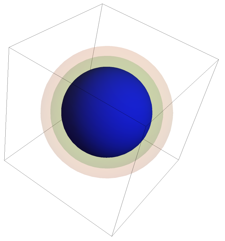
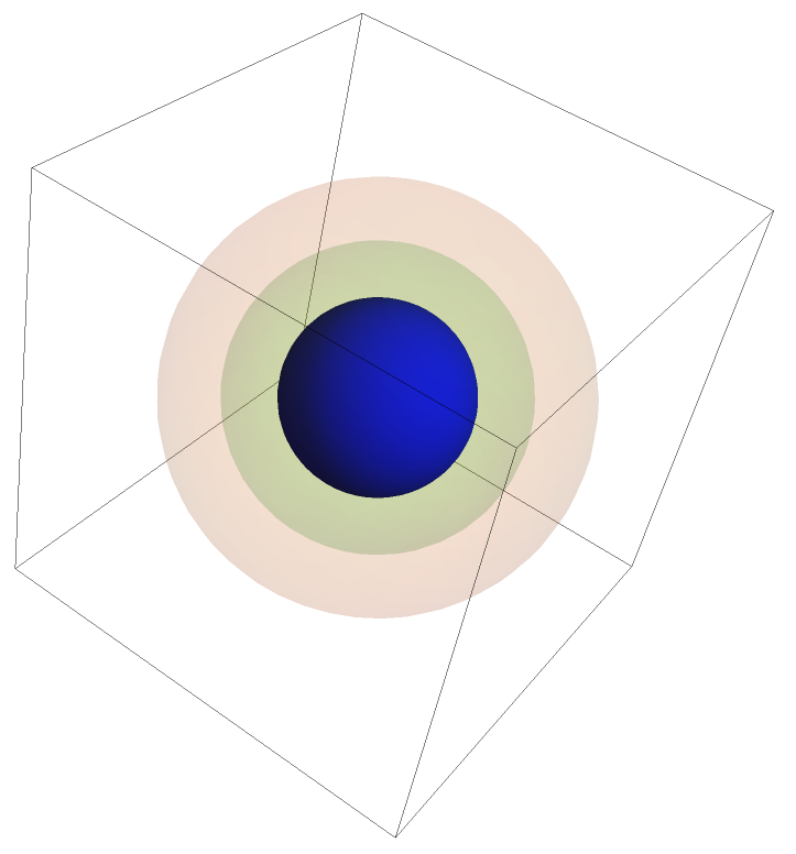
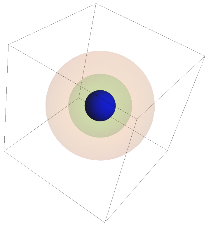
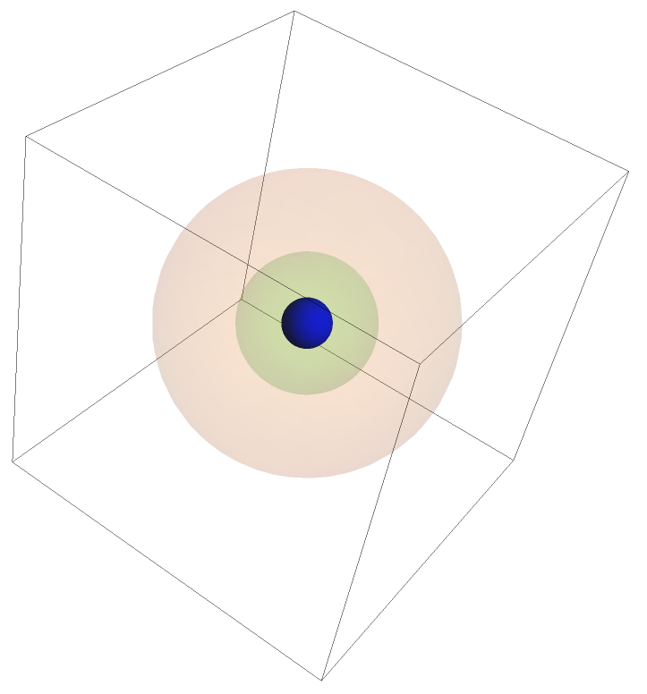
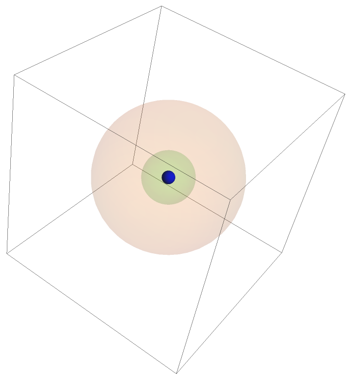
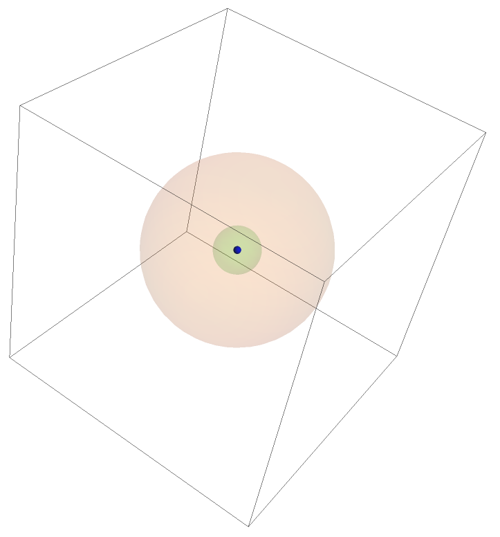
Figure 1. Schematic representation of the geometry of cell and inclusions in the limiting supercritical, critical, and subcritical cases. The elementary cell with side length $\varepsilon$ rescaled to unit is drawn in order to have comparable pictures. For $n=3$, the blue, the green, and the orange spheres represent the inclusion centered at the center of the cell respectively in the subcritical $\eta(\varepsilon)=(\varepsilon^{2/(n-2)})^{2}$, critical $\eta(\varepsilon)=\varepsilon^{2/(n-2)}$, and supercritical $\eta(\varepsilon)=(\varepsilon^{2/(n-2)})^{1/4}$ cases. In lexicographic order $\varepsilon=0.9,0.8,0.7,0.6,0.5,0.4$.

First asymptotic scheme. We first let $\delta\to 0$ and then consider the homogenization limit $\varepsilon\to 0$. To this end in Section 3.1 we find the limit problem for $\delta\to 0$ in Theorem 3.2 and call it the degenerate problem. Then, in Section 5 we homogenize the degenerate problem, but different choices for the behavior of the relative inclusion size $\eta$ can be considered when $\varepsilon\to 0$. In Section 5.1 we consider the so called critical case $\eta\approx\varepsilon^{2/(n-2)}$, see [16]. The supercritical $\eta\gg\varepsilon^{2/(n-2)}$ and the subcritical $\eta\ll\varepsilon^{2/(n-2)}$ cases are treated, respectively, in Section 5.2 and 5.3.

Second asymptotic scheme. We fix $\delta>0$ and consider the homogenization limit $\varepsilon\to 0$ in Sections  6.1 and 6.2. Such a limit depends on how $\eta$ and $\varepsilon$ are related, so the homogenization study is indeed divided into two parts: in Section 6.1 we consider $\eta=\eta(\varepsilon)$ tending to zero as $\varepsilon\to 0$, while in Section 6.2 we assume $\eta$ constant. Then we pass to the limit $\delta\to 0$ in Section 6.3.

We can summarize our results saying that, according to the dependence of the relative size $\eta$ on the cell size $\varepsilon$, we find three possible behaviors for the upscaled equations: pure diffusion, diffusion with mass deposition, and absence of diffusion. More precisely, for what concerns the first asymptotic scheme, in Section 3, the problems (3.8)–(3.11) and (3.13)–(3.14) are found, respectively, outside and inside the inclusions in the degeneration limit $\delta\to 0$. The former is a standard Fokker–Planck problem with homogeneous Dirichlet condition on the inclusions boundary. The latter is an ordinary differential equation in time with a source term, which can be equivalently rewritten as equation (3.15). It is to remark that the convergence to the solution of the limit problem as $\delta\to 0$ inside the inclusions can be proven only on compact subdomains, since close to the inclusions boundary a phenomenon of mass concentration takes place. Indeed, in Theorem 3.5 we show that the total mass in a vanishingly small strip adjacent from the inside to the inclusions boundary tends, in the degeneration limit, to the total mass flux arriving to the boundary from the exterior.

When in Section 5 we homogenize the degenerate equations derived in Section 3, we find different upscaled systems depending on the way in which the relative size of the inclusions $\eta$ is scaled with respect to the cell size $\varepsilon$. Referring to the nomenclature introduced above, in the subcritical regime inclusions have a poor effect and a standard Fokker–Planck diffusion problem is found in Theorem 5.9 with diffusion coefficient provided by a suitable cell average of the original coefficient. In the critical case, as in the pioneering paper [16], inclusions are effective and yield a positive capacitary term in the diffusion equation of Theorem 5.4 accounting for mass deposition. Finally, in the supercritical case, as shown in Theorem 5.6, inclusions dominate and, provided the mass concentration phenomenon is correctly taken into account, the mass density converges to the solution of an ordinary differential equation in time as $\varepsilon$ tends to zero.

For what concerns the second asymptotic scheme, we have to consider two different cases. When the relative size $\eta$ tends to zero as $\varepsilon\to 0$, in Theorem 6.2 we prove that the limit solution solves the standard Fokker–Planck diffusion problem (5.44) which does not depend on the degeneration parameter, so that no further analysis is needed. On the other hand, if the relative size is kept constant, say $\eta=1$, in Theorem 6.4 we prove that, as $\varepsilon\to 0$, the limit solution solves the standard Fokker–Planck diffusion problem (6.14) with diffusion coefficient depending on the degeneration parameter $\delta$. Moreover, as proven in Theorem 6.5, its solution, in the limit $\delta\to 0$, tends to the solution of the ordinary differential equation (3.15).

We remark that the computation that we perform in Section 5 is valid only in dimension $n\geq 3$, since we follow the ideas in [15] which are not valid in smaller dimensions. On the contrary, the results discussed in Sections 3 and 6 are in force for any dimension $n\geq 2$.

Finally, we note that, since in the two schemes the degeneration and the homogenization limits are taken in reversed order, it is natural to compare these results each other and look for possible commutation properties. We refer to Remark 6.6 for a thorough discussion, but, here, we anticipate that the two strategies commute when $\eta=1$, whereas when $\eta\to 0$ as $\varepsilon\to 0$ they commute in the subcritical case, while in the critical and supercritical cases they do not.

In view of the variety of these results, a natural question arises about the behavior of the model when the degeneration and the homogenization limits are taken simultaneously, namely, when the parameter $\delta$ is considered a vanishing function of $\varepsilon$. Preliminary results suggest that this can be a promising study and, thus, it will be the topic of future research.

The paper is organized as follows. In Section 2 we introduce the model. In Section 3 we discuss the degeneration $\delta\to 0$ limit. Section 4 is devoted to a short review of the unfolding approach to homogenization. In Sections 5 and 6 we study, respectively, the homogenization limit of the degenerate and the non–degenerate problems. In Section 7 we provide an explicit solution of the problem under investigation in the one–dimensional case showing that, if one considered diffusion coefficient depending on time, globally bounded solutions could not exist. Finally, in Section 8 we summarize our conclusions.

2. The problem

Let $\varOmega\subset\mathbb{R}^{n}$ be a smooth bounded open set. Let $\varepsilon>0$ be a small parameter denoting the length scale of the periodic microstructure. Let us consider the tiling of $\mathbb{R}^{n}$ given by the boxes $\varepsilon(\xi+\mathcal{Y})$, with $\xi\in\mathbb{Z}^{n}$ and $\mathcal{Y}=(-1/2,1/2)^{n}$. We denote by $[r]$ the integer part of $r\in\mathbb{R}$ with respect to the reference cell $(-1/2,1/2)$ (i.e., $[r]=k\in\mathbb{Z}$ if and only if $r\in[k-1/2,k+1/2)$) and, similarly, we denote by $\{r\}=r-[r]$, i.e., the fractional part of $r$ with respect to $(-1/2,1/2)$. Moreover, for $x\in\mathbb{R}^{n}$, we define the vector with integer components $[x]_{\mathcal{Y}}=([x_{1}],\dots,[x_{n}])$. We refer to Fig. 2 for a schematic representation of the geometric setup.

We set

$$\Xi_{\varepsilon}=\{\xi\in\mathbb{Z}^{n}:\,\varepsilon(\xi+\mathcal{Y})\subset\Omega\},\ \hat{\Omega}_{\varepsilon}=\text{interior}\Big{\{}\bigcup_{\xi\in\Xi_{\varepsilon}}\varepsilon(\xi+\overline{\mathcal{Y}})\Big{\}},$$ (2.1)

$$\hphantom{jhkfgjdhsaJ,KHGFD}\Lambda_{\varepsilon}=\Omega\setminus\hat{\Omega}_{\varepsilon}\;.$$

We introduce also the scaled cell containing the point $x$ as

$$\mathcal{Y}_{\varepsilon}(x)=\varepsilon\left(\left[\frac{x}{\varepsilon}\right]_{\mathcal{Y}}+\mathcal{Y}\right)\,.$$

In the sequel, we will assume that $\varOmega$ contains an $\varepsilon\mathcal{Y}$-periodic array of smooth small holes of size $\eta\varepsilon$ ($1\geq\eta>0$ possibly depending on $\varepsilon$). More precisely, if the reference inclusion (also called hole, as in the previous literature) $B\subset\subset\mathcal{Y}$ is a given connected regular open set, we denote by $\mathcal{Y}^{*}_{\eta}=\mathcal{Y}\setminus\eta\overline{B}$ and define $\varOmega^{*}_{\varepsilon,\eta}$ as

$$\varOmega^{*}_{\varepsilon,\eta} =\hbox{interior}\left\{\bigcup_{\xi\in\Xi_{\varepsilon}}\varepsilon(\xi+\overline{\mathcal{Y}}^{*}_{\eta})\right\}$$ (2.2)

$$=\left\{x\in\hat{\varOmega}_{\varepsilon},\ \hbox{such that\ }\frac{x}{\varepsilon}-\left[\frac{x}{\varepsilon}\right]_{\mathcal{Y}}\in\mathcal{Y}^{*}_{\eta}\right\}.$$

We also denote by $\varOmega^{1}_{\varepsilon}=\hat{\varOmega}_{\varepsilon}\setminus\overline{\varOmega^{*}_{\varepsilon,\eta}}=\cup_{\xi\in\Xi_{\varepsilon}}\varepsilon(\xi+\eta B)$ and $\varOmega^{2}_{\varepsilon}=\Lambda_{\varepsilon}\cup\varOmega^{*}_{\varepsilon,\eta}=\varOmega\setminus\overline{\varOmega^{1}_{\varepsilon}}$, respectively, and we assume that, for every $\varepsilon>0$, they are smooth sets. For the sake of simplicity, we also denote by $\varGamma_{\varepsilon}=\partial\varOmega^{2}_{\varepsilon}\setminus\partial\varOmega=\partial\varOmega^{1}_{\varepsilon}$, so that $\varOmega=\varOmega^{1}_{\varepsilon}\cup\varOmega^{2}_{\varepsilon}\cup\varGamma_{\varepsilon}$; that is $\varOmega^{1}_{\varepsilon}$ is the interior of the inclusions and $\varOmega^{2}_{\varepsilon}$ is the outer domain.

Figure 2. Schematic description of the geometry of the model in dimension $n=2$ and some related notions. The gray dots represent the inclusions. Left: tiling and definition of integer part $[x]_{\mathcal{Y}}=(k_{1},k_{2})$. On the right the lattice is rescaled with $\varepsilon=1/2$ and $\eta=1$: the big circle represents the open set $\Omega$ and the region with solid boundary is the set $\bigcup_{\xi\in\Xi_{\varepsilon}}\varepsilon(\xi+\overline{\mathcal{Y}})$.

Finally, for any set $\mathcal{G}\subset\mathbb{R}^{n}$, we denote $\mathcal{G}_{T}=\mathcal{G}\times(0,T)$.

Let us consider the problem

$$\frac{\partial u_{\varepsilon,\delta}}{\partial t}-\operatorname{\Delta}(b_{\varepsilon,\delta}u_{\varepsilon,\delta}) =f\,, \varOmega_{T}$$ in ; (2.3)

$$\frac{\partial(b_{\varepsilon,\delta}u_{\varepsilon,\delta})}{\partial\nu} =0\,, \partial\varOmega\times(0,T)$$ on ; (2.4)

$$u_{\varepsilon,\delta}(x,0) =\bar{u}(x)\,, \varOmega$$ in . (2.5)

Here $\nu$ denotes the outer normal to $\partial\varOmega$, $f\in L^{2}(\varOmega_{T})$, $\bar{u}\in L^{2}(\varOmega)$. For $0<\delta\leq 1$ and $\varepsilon>0$

$$b_{\varepsilon,\delta}(x)=\left\{\begin{aligned} &\delta b_{\varepsilon}(x)\,,&\qquad&x\in\varOmega^{1}_{\varepsilon}\,;\\ &b_{\varepsilon}(x)\,,&\qquad&x\in\varOmega^{2}_{\varepsilon}\,,\end{aligned}\right.$$ (2.6)

with $b_{\varepsilon}(x)=b(x,x/\varepsilon)$, where $b$ is a Carathéodory function belonging to $L^{\infty}(\varOmega\times\mathcal{Y})$, which is $\mathcal{Y}$-periodic with respect to the second variable and satisfies

$$b(x,y)\geq C>0\,,\qquad(x,y)\in\varOmega\times\mathcal{Y}\,,$$ (2.7)

for a suitable constant $C>0$.

Notice that, as explained in the Introduction, the appearance of two small parameters $\varepsilon$ and $\delta$ in problem (2.3)–(2.5) leads us to consider, and compare, the behavior of the problem when we let first $\delta\to 0$ and then $\varepsilon\to 0$ or vice versa. These situations will be analyzed in the following sections.

Definition 2.1.

A weak solution to problem (2.3)–(2.5) is a function $u_{\varepsilon,\delta}\in H^{1}(t_{0},T;L^{2}(\varOmega))\cap\mathcal{C}([0,T];L^{2}(\varOmega))$ for all $0<t_{0}<T$, such that $b_{\varepsilon,\delta}u_{\varepsilon,\delta}\in L^{2}(0,T;H^{1}(\varOmega))$ and

$$\int_{\varOmega_{T}}\Big{[}\frac{\partial u_{\varepsilon,\delta}}{\partial t}\varphi+\operatorname{\nabla}(b_{\varepsilon,\delta}u_{\varepsilon,\delta})\operatorname{\nabla}\varphi\Big{]}\,\textup{{d}}x\,\textup{{d}}t=\int_{\varOmega_{T}}f\varphi\,\textup{{d}}x\,\textup{{d}}t\,,$$ (2.8)

for all $\varphi\in L^{2}(0,T;H^{1}(\varOmega))$, with support bounded away from $t=0$. In addition, we require $u_{\varepsilon,\delta}=\bar{u}$ at time $t=0$ in the $L^{2}$ sense. ∎

We may give to (2.8) the equivalent alternative formulation

$$-\int_{\varOmega_{T}}u_{\varepsilon,\delta}\phi_{t}\,\textup{{d}}x\,\textup{{d}}t+\int_{\varOmega_{T}}\operatorname{\nabla}(b_{\varepsilon,\delta}u_{\varepsilon,\delta})\operatorname{\nabla}\phi\,\textup{{d}}x\,\textup{{d}}t\\ =\int_{\varOmega_{T}}f\phi\,\textup{{d}}x\,\textup{{d}}t+\int_{\varOmega}\bar{u}(x)\phi(x,0)\,\textup{{d}}x\,,$$ (2.9)

for all test functions $\phi\in H^{1}(\varOmega_{T})$, with $\phi(x,T)=0$ in $\varOmega$, in the sense of traces. For example we may choose for any $\varphi\in\mathcal{C}^{1}(\overline{\varOmega_{T}})$

$$\phi(x,t)=\int_{t}^{T}\varphi(x,\tau)\,\textup{{d}}\tau\,.$$ (2.10)

2.1. Energy and $L^{1}$ estimates

Here we collect some results which are used throughout the paper.

An immediate consequence of (2.8) is the balance

$$\int_{\varOmega}u_{\varepsilon,\delta}(x,t)\,\textup{{d}}x=\int_{\varOmega}\bar{u}(x)\,\textup{{d}}x+\int_{0}^{t}\int_{\varOmega}f(x,\tau)\,\textup{{d}}x\,\textup{{d}}\tau\,,\quad 0<t<T\,.$$ (2.11)

We infer by (2.8) and routine arguments the energy estimate

$$\sup_{0<t<T}\int_{\varOmega}b_{\varepsilon,\delta}u_{\varepsilon,\delta}(t)^{2}\,\textup{{d}}x+\int_{\varOmega_{T}}\lvert\operatorname{\nabla}(b_{\varepsilon,\delta}u_{\varepsilon,\delta})\rvert^{2}\,\textup{{d}}x\,\textup{{d}}t\\ \leq\gamma(T)\Big{(}\int_{\varOmega}b_{\varepsilon,\delta}\bar{u}^{2}\,\textup{{d}}x+\int_{\varOmega_{T}}b_{\varepsilon,\delta}f^{2}\,\textup{{d}}x\,\textup{{d}}t\Big{)}\,,$$ (2.12)

where, here and in the following, $\gamma$ is a generic positive real number not depending on $\varepsilon$, $\delta$, and $\eta$.

We also have, from (2.8) and (2.12), by choosing as test function the product of $b_{\varepsilon,\delta}\partial u_{\varepsilon,\delta}/\partial t$ times a continuous function of time constant for $t\geq t_{0}$ and zero in $0$, that for all $0<t_{0}<T$

$$\int_{t_{0}}^{T}\int_{\varOmega}b_{\varepsilon,\delta}\Big{(}\frac{\partial u_{\varepsilon,\delta}}{\partial t}\Big{)}^{2}\,\textup{{d}}x\,\textup{{d}}t+\sup_{t_{0}<t<T}\int_{\varOmega}\lvert\operatorname{\nabla}(b_{\varepsilon,\delta}u_{\varepsilon,\delta}(t))\rvert^{2}\,\textup{{d}}x\\ \leq\gamma(T)t_{0}^{-1}\Big{(}\int_{\varOmega}b_{\varepsilon,\delta}\bar{u}^{2}\,\textup{{d}}x+\int_{\varOmega_{T}}b_{\varepsilon,\delta}f^{2}\,\textup{{d}}x\,\textup{{d}}t\Big{)}\,.$$ (2.13)

Such estimates may be used to prove existence of a solution in the sense of Definition 2.1, via approximation with smoothed problems, and also its uniqueness, since the problem is linear. Alternatively, uniqueness follows from our next result.

Lemma 2.2 (Conservation of mass).

We have for all $t\in(0,T)$

$$\int_{\varOmega}\lvert u_{\varepsilon,\delta}(x,t)\rvert\,\textup{{d}}x\leq\int_{\varOmega}\lvert\bar{u}(x)\rvert\,\textup{{d}}x+\int_{0}^{t}\int_{\varOmega}\lvert f\rvert\,\textup{{d}}x\,\textup{{d}}\tau\,.$$ (2.14)

If $\bar{u}\geq 0$, $f\geq 0$ then $u_{\varepsilon,\delta}\geq 0$ and, if in addition $f=0$,

$$\lVert u_{\varepsilon,\delta}(t)\rVert_{L^{1}(\varOmega)}=\lVert\bar{u}\rVert_{L^{1}(\varOmega)}\,,\qquad 0<t<T\,.$$ (2.15)

Proof.

Let $\operatorname{sign}_{\sigma}$ be a smoothed increasing version of the sign function, with $\operatorname{sign}_{\sigma}(0)=0$, converging everywhere to $\operatorname{sign}$ as $\sigma\to 0+$, and select as a testing function in (2.8) $\operatorname{sign}_{\sigma}(b_{\varepsilon,\delta}u_{\varepsilon,\delta})\chi_{(t_{0},t)}(\tau)$. We get

$$\int_{t_{0}}^{t}\int_{\varOmega}\Big{[}\frac{\partial u_{\varepsilon,\delta}}{\partial\tau}\operatorname{sign}_{\sigma}(b_{\varepsilon,\delta}u_{\varepsilon,\delta})+\operatorname{sign}_{\sigma}^{\prime}(b_{\varepsilon,\delta}u_{\varepsilon,\delta})\lvert\operatorname{\nabla}(b_{\varepsilon,\delta}u_{\varepsilon,\delta})\rvert^{2}\Big{]}\,\textup{{d}}x\,\textup{{d}}\tau\\ \leq\int_{t_{0}}^{t}\int_{\varOmega}\lvert f\rvert\,\textup{{d}}x\,\textup{{d}}\tau\,.$$

Next we drop the non-negative term on the left hand side, then we let $\sigma\to 0+$ and note that $\operatorname{sign}(b_{\varepsilon,\delta}u_{\varepsilon,\delta})=\operatorname{sign}(u_{\varepsilon,\delta})$; thus we obtain

$$\int_{t_{0}}^{t}\int_{\varOmega}\lvert f\rvert\,\textup{{d}}x\,\textup{{d}}\tau\geq\int_{t_{0}}^{t}\int_{\varOmega}\frac{\partial u_{\varepsilon,\delta}}{\partial\tau}\operatorname{sign}(u_{\varepsilon,\delta})\,\textup{{d}}x\,\textup{{d}}\tau\\ =\int_{t_{0}}^{t}\int_{\varOmega}\frac{\partial\lvert u_{\varepsilon,\delta}\rvert}{\partial\tau}\,\textup{{d}}x\,\textup{{d}}\tau=\int_{\varOmega}\lvert u_{\varepsilon,\delta}(x,t)\rvert\,\textup{{d}}x-\int_{\varOmega}\lvert u_{\varepsilon,\delta}(x,t_{0})\rvert\,\textup{{d}}x\,.$$

On letting $t_{0}\to 0$ we arrive at (2.14).

The positivity result follows similarly, by replacing $\operatorname{sign}_{\sigma}(s)$ with $\operatorname{sign}_{\sigma}(s)\chi_{(-\infty,0)}(s)$; then (2.15) follows from (2.11). ∎

2.2. An auxiliary formulation.

If we set $v_{\varepsilon,\delta}=b_{\varepsilon,\delta}u_{\varepsilon,\delta}$ we obtain for this new unknown the problem

$$\frac{1}{b_{\varepsilon,\delta}}\frac{\partial v_{\varepsilon,\delta}}{\partial t}-\operatorname{\Delta}v_{\varepsilon,\delta} =f\,, \varOmega_{T}$$ in ; (2.16)

$$\frac{\partial v_{\varepsilon,\delta}}{\partial\nu} =0\,, \partial\varOmega\times(0,T)$$ on ; (2.17)

$$v_{\varepsilon,\delta}(x,0) =b_{\varepsilon,\delta}(x)\bar{u}(x)\,, \varOmega$$ in . (2.18)

The weak formulations follow obviously from the ones in Definition 2.1 and in (2.9); let us write explicitly the latter form as

$$-\int_{\varOmega_{T}}\frac{v_{\varepsilon,\delta}}{b_{\varepsilon,\delta}}\phi_{t}\,\textup{{d}}x\,\textup{{d}}t+\int_{\varOmega_{T}}\operatorname{\nabla}v_{\varepsilon,\delta}\operatorname{\nabla}\phi\,\textup{{d}}x\,\textup{{d}}t\\ =\int_{\varOmega_{T}}f\phi\,\textup{{d}}x\,\textup{{d}}t+\int_{\varOmega}\bar{u}(x)\phi(x,0)\,\textup{{d}}x\,,$$ (2.19)

for all test functions $\phi\in H^{1}(\varOmega_{T})$, with $\phi(x,T)=0$ in $\varOmega$, in the sense of traces.

From the estimates (2.12) and (2.13) we obtain for all $0<t_{0}<T$

$$\sup_{0<t<T}\int_{\varOmega}\frac{v_{\varepsilon,\delta}(t)^{2}}{b_{\varepsilon,\delta}}\,\textup{{d}}x+\int_{\varOmega_{T}}\lvert\operatorname{\nabla}v_{\varepsilon,\delta}\rvert^{2}\,\textup{{d}}x\,\textup{{d}}t+t_{0}\int_{t_{0}}^{T}\int_{\varOmega}\frac{1}{b_{\varepsilon,\delta}}\Big{(}\frac{\partial v_{\varepsilon,\delta}}{\partial t}\Big{)}^{2}\,\textup{{d}}x\,\textup{{d}}t\leq\gamma\,,$$ (2.20)

with $\gamma$ as above and independent of $t_{0}$.

Remark 2.3.

As a consequence of (2.20), the sequence $v_{\varepsilon,\delta}$ is compact in $L^{2}(\varOmega_{T})$ and we have, up to subsequences for $\varepsilon\to 0$ and $\delta\to 0$,

$$v_{\varepsilon,\delta} \to v_{0}\,, L^{2}(\varOmega_{T})$$ strongly in ; (2.21)

$$\operatorname{\nabla}v_{\varepsilon,\delta} \rightharpoonup\operatorname{\nabla}v_{0}\,, L^{2}(\varOmega_{T})$$ weakly in ; (2.22)

$$\frac{\partial v_{\varepsilon,\delta}}{\partial t} \rightharpoonup\frac{\partial v_{0}}{\partial t}\,, L^{2}(\varOmega\times(t_{0},T)) t_{0}>0$$ weakly in , for all . (2.23)

∎

Remark 2.4 ($L^{\infty}$ bounds for $b_{\varepsilon,\delta}$ independent of time).

It is possible to prove (see, [7]) that, if for example $f=0$ and $\bar{u}\geq 0$,

$$0\leq u_{\varepsilon,\delta}(x,t)\leq\frac{\sup_{\varOmega}b_{\varepsilon,\delta}}{\inf_{\varOmega}b_{\varepsilon,\delta}}\,\sup_{\varOmega}\bar{u}\,,\qquad(x,t)\in\varOmega_{T}\,.$$ (2.24)

This result relies on the independence of $b_{\varepsilon,\delta}$ from time: see Section 7 for further comments and a counterexample motivating our choice $b_{\varepsilon,\delta}=b_{\varepsilon,\delta}(x)$ independent on time in this paper.

However, we note that the definitions of weak solutions (2.8), (2.9), and (2.19) would be still valid even if $b_{\varepsilon,\delta}$ depended on time. ∎

3. The degeneration limit of the Fokker–Planck problem

In this section, we will assume $\varepsilon$ fixed (i.e., $\varepsilon=1$) and study the behavior of the solution with respect to $\delta\to 0$. For this reason, we will omit the subscript index $\varepsilon$ and replace $\varOmega^{1}_{\varepsilon}$, $\varOmega^{2}_{\varepsilon}$, and $\Gamma_{\varepsilon}$ with $\varOmega^{1}$, $\varOmega^{2}$, and $\Gamma$, respectively. Moreover, we will use the superscripts “in” and “out” to denote restrictions to $\varOmega^{1}$ and $\varOmega^{2}$.

Since, the spatial periodicity of cavities is not important in this section, we can just assume that the smooth bounded open sets $\varOmega^{1}$ and $\varOmega^{2}$ satisfy the following assumptions: $\varOmega^{1}\subset\overline{\varOmega^{1}}\subset\varOmega$ and $\varOmega^{2}=\varOmega\setminus\overline{\varOmega^{1}}$. We also let $u_{\delta}=u_{\varepsilon,\delta}$, $v_{\delta}=v_{\varepsilon,\delta}$, and $b_{\delta}=b_{\varepsilon,\delta}$.

We stress that we will rely on some non-standard energy estimates where the tracking of the behavior in $\delta$ is rather delicate (see especially Lemma 3.3).

First of all we note that standard arguments and the assumed regularity of $b_{\delta}u_{\delta}$ imply that a weak solution to (2.3)–(2.5), which is smooth enough in $\varOmega^{1}$ and in $\varOmega^{2}$, satisfies

$$\frac{\partial u_{\delta}}{\partial t}-\delta\operatorname{\Delta}(bu_{\delta}) =f\,, \varOmega^{1}_{T}$$ in ; (3.1)

$$\frac{\partial u_{\delta}}{\partial t}-\operatorname{\Delta}(bu_{\delta}) =f\,, \varOmega^{2}_{T}$$ in ; (3.2)

$$\frac{\partial(bu_{\delta})}{\partial\nu} =0\,, \partial\varOmega\times(0,T)$$ on ; (3.3)

$$[b_{\delta}u_{\delta}] =0\,, \varGamma_{T}$$ on ; (3.4)

$$[\operatorname{\nabla}(b_{\delta}u_{\delta})\cdot n] =0\,, \varGamma_{T}$$ on ; (3.5)

$$u_{\delta}(x,0) =\bar{u}(x)\,, \varOmega$$ in . (3.6)

Recall that $\varGamma=\partial\varOmega^{1}\cap\partial\varOmega^{2}$ and $n$ is the normal to $\varGamma$ pointing into $\varOmega^{2}$. Let us remark that (3.4) follows from the fact that $b_{\delta}u_{\delta}$ is a Sobolev function and (3.5) is a standard consequence of the differential equation (2.3) understood in a distributional sense. Note, also, that (3.4) implies that $u_{\delta}$ is not continuous across the interface $\Gamma$.

3.1. The limit degenerate problem

The point of the following estimate is that it is independent of $\delta$ (excepting the factor in the second integral of (3.7)).

Lemma 3.1.

For all $\varphi\in\mathcal{C}^{1}_{0}(\varOmega^{1})$, $0\leq\varphi\leq 1$, we have

$$\sup_{0<t<T}\int_{\varOmega^{1}}bu_{\delta}(t)^{2}\varphi^{2}\,\textup{{d}}x+\delta\int_{0}^{t}\int_{\varOmega^{1}}\lvert\operatorname{\nabla}(bu_{\delta})\rvert^{2}\varphi^{2}\,\textup{{d}}x\,\textup{{d}}\tau\\ \leq\gamma(1+\lVert\operatorname{\nabla}\varphi\rVert_{\infty}^{2})\Big{(}\int_{\varOmega}\bar{u}^{2}\,\textup{{d}}x+\int_{\varOmega_{T}}f^{2}\,\textup{{d}}x\,\textup{{d}}t\Big{)}\,.$$ (3.7)

Here $\gamma$ depends on $T$.

Proof.

The proof is based on standard arguments that we report for the reader’s convenience. Indeed, select $\varphi^{2}bu_{\delta}\chi_{[t_{0},t]}(\tau)$ as a testing function in (2.8), integrate by parts and let $t_{0}\to 0+$ to get

$$\!\!\!\frac{1}{2}\int_{\varOmega^{1}}bu_{\delta}(t)^{2}\varphi^{2}\,\textup{{d}}x+\delta\int_{0}^{t}\int_{\varOmega^{1}}\lvert\operatorname{\nabla}(bu_{\delta})\rvert^{2}\varphi^{2}\,\textup{{d}}x\,\textup{{d}}\tau\\ \;=\frac{1}{2}\int_{\varOmega^{1}}b\bar{u}^{2}\varphi^{2}\,\textup{{d}}x+2\delta\int_{0}^{t}\int_{\varOmega^{1}}\operatorname{\nabla}(bu_{\delta})\operatorname{\nabla}\varphi\varphi u_{\delta}b\,\textup{{d}}x\,\textup{{d}}\tau+\int_{0}^{t}\int_{\varOmega^{1}}f\varphi^{2}u_{\delta}b\,\textup{{d}}x\,\textup{{d}}\tau\,.$$

The sum of the last two integrals is bounded from above by

$$\frac{\delta}{2}\int_{0}^{t}\int_{\varOmega^{1}}\lvert\operatorname{\nabla}(bu_{\delta})\rvert^{2}\varphi^{2}\,\textup{{d}}x\,\textup{{d}}\tau+2\delta\int_{0}^{t}\int_{\varOmega^{1}}\lvert\operatorname{\nabla}\varphi\rvert^{2}u_{\delta}^{2}b^{2}\,\textup{{d}}x\,\textup{{d}}\tau\\ +\int_{0}^{t}\int_{\varOmega^{1}}f^{2}\varphi^{2}\,\textup{{d}}x\,\textup{{d}}\tau+\int_{0}^{t}\int_{\varOmega^{1}}u_{\delta}^{2}\varphi^{2}b^{2}\,\textup{{d}}x\,\textup{{d}}\tau\,.$$

By taking into account (2.12) we infer that

$$\int_{\varOmega^{1}}u_{\delta}(t)^{2}\varphi^{2}b\,\textup{{d}}x+\delta\int_{0}^{t}\int_{\varOmega^{1}}\lvert\operatorname{\nabla}(bu_{\delta})\rvert^{2}\varphi^{2}\,\textup{{d}}x\,\textup{{d}}\tau\\ \leq\gamma(1+\lVert\operatorname{\nabla}\varphi\rVert_{\infty}^{2})\Big{(}\int_{\varOmega}\bar{u}^{2}\,\textup{{d}}x+\int_{0}^{t}\int_{\varOmega}f^{2}\,\textup{{d}}x\,\textup{{d}}t\Big{)}+\gamma\int_{0}^{t}\int_{\varOmega^{1}}u_{\delta}^{2}\varphi^{2}b\,\textup{{d}}x\,\textup{{d}}t\,.$$

The claim follows after an application of Gronwall’s lemma. ∎

Next we show that as $\delta\to 0$, $u_{\delta}$ converges, in the respective spatial domains, to the solutions of the two following problems. The problem in the outer domain $\varOmega^{2}$ is

$$\frac{\partial u}{\partial t}-\operatorname{\Delta}(bu) =f\,, \varOmega^{2}_{T}$$ in ; (3.8)

$$\frac{\partial(bu)}{\partial\nu} =0\,, \partial\varOmega\times(0,T)$$ on ; (3.9)

$$bu =0\,, \varGamma_{T}$$ on ; (3.10)

$$u(x,0) =\bar{u}(x)\,, \varOmega^{2}$$ in . (3.11)

Problem (3.8)–(3.11) has the standard weak formulation: Find $u\in L^{2}(\varOmega_{T})$, with $bu\in L^{2}(0,T;H^{1}(\varOmega))$ and satisfying (3.10), such that

$$\int_{\varOmega^{2}_{T}}\Big{[}-u\frac{\partial\varphi}{\partial t}+\operatorname{\nabla}(bu)\operatorname{\nabla}\varphi\Big{]}\,\textup{{d}}x\,\textup{{d}}t=\int_{\varOmega^{2}}\bar{u}\varphi(0)\,\textup{{d}}x+\int_{\varOmega^{2}_{T}}f\varphi\,\textup{{d}}x\,\textup{{d}}t\,,$$ (3.12)

for all $\varphi\in H^{1}(\varOmega^{2}_{T})$, with $\varphi=0$ on $\varGamma$ and at $t=T$.

The problem in the interior domain $\varOmega^{1}$ is: Find $u$ such that $u$, $\partial u/\partial t\in L^{2}(\varOmega^{1}_{T})$ and

$$\frac{\partial u}{\partial t} =f\,, L^{2}(\varOmega^{1}_{T})$$ in ; (3.13)

$$u(x,0) =\bar{u}(x)\,, \varOmega^{1}$$ in , in the sense of traces. (3.14)

In fact, it is easy to prove that (3.13)–(3.14) can be written equivalently as $u=F$ in $\varOmega^{1}$ where

$$F(x,t)=\bar{u}(x)+\int_{0}^{t}f(x,\tau)\,\textup{{d}}\tau\,,\qquad(x,t)\in\varOmega_{T}\,.$$ (3.15)

Theorem 3.2.

As $\delta\to 0$, for every fixed $t_{0}>0$,

$$u_{\delta} \to u\,,\qquad L^{2}(\varOmega^{2}_{T})$$ strongly in ; (3.16)

$$\operatorname{\nabla}(bu_{\delta}) \rightharpoonup\operatorname{\nabla}(bu)\,,\qquad L^{2}(\varOmega^{2}_{T})$$ weakly in ;

$$\frac{\partial u_{\delta}}{\partial t} \rightharpoonup\frac{\partial u}{\partial t}\,,\qquad L^{2}(\varOmega^{2}\times(t_{0},T))$$ weakly in ,

for a suitable $u\in L^{2}(\varOmega^{2}_{T})$. In addition

$$u_{\delta}\rightharpoonup u\,,\qquad\textup{weakly in $L^{2}(0,T;L^{2}_{\textup{{loc}}}(\varOmega^{1}))$,}$$ (3.17)

for a suitable $u\in L^{2}_{\textup{{loc}}}(\varOmega^{1}\times[0,T])$.

The limits of $u_{\delta}$ solve the problems (3.8)–(3.11) and (3.13)–(3.14) respectively.

Proof.

Let us recall the notation $v_{\delta}=b_{\delta}u_{\delta}$, i.e., $v_{\delta}=bu_{\delta}$ in $\varOmega^{2}_{T}$, and setting $u=v/b$ in $\varOmega^{2}_{T}$, as a consequence of Remark 2.3 we have (3.16).

Next we show that $u$ solves in the weak sense (3.8)–(3.11). First note that the function $v_{\delta}/\sqrt{b_{\delta}}$ converges weakly in $L^{2}(\varOmega_{T})$, owing to (2.20). Therefore, $v=0$ in $\varOmega^{1}_{T}$, i.e., $v_{\delta}$, $\operatorname{\nabla}v_{\delta}\rightharpoonup 0$ weakly in $L^{2}(\varOmega^{1}_{T})$.

Thus, by continuity of traces, as $\delta\to 0$,

$$0=[b_{\delta}u_{\delta}]=v_{\delta}^{\textup{{out}}}{}_{\mid\varGamma}-v_{\delta}^{\textup{{int}}}{}_{\mid\varGamma}\to v^{\textup{{out}}}{}_{\mid\varGamma}=(bu)^{\textup{{out}}}{}_{\mid\varGamma}\,.$$ (3.18)

This proves (3.10).

Moreover, in (2.8) take $\varphi\in H^{1}(\varOmega^{2}_{T})$, with $\varphi=0$ on $\varGamma$ and at $t=T$ and extend to $0$ in $\varOmega^{1}_{T}$. We obtain

$$\int_{\varOmega^{2}_{T}}\Big{[}-u_{\delta}\frac{\partial\varphi}{\partial t}+\operatorname{\nabla}(bu_{\delta})\operatorname{\nabla}\varphi\Big{]}\,\textup{{d}}x\,\textup{{d}}t=\int_{\varOmega^{2}}\bar{u}\varphi(0)\,\textup{{d}}x+\int_{\varOmega^{2}_{T}}f\varphi\,\textup{{d}}x\,\textup{{d}}t\,.$$ (3.19)

As $\delta\to 0$ we get (3.12).

As to the problem in the interior domain $\varOmega^{1}$, we remark that from (3.7) our claim (3.17) follows.

Next, we prove that $u$ solve (3.13)–(3.14) weakly. Consider $\varphi\in\mathcal{C}^{1}(\varOmega^{1}_{T})$ and such that its support is bounded away from $\partial\varOmega^{1}$ and $t=T$. From (2.8) we have

$$\int_{\varOmega^{1}_{T}}f\varphi\,\textup{{d}}x\,\textup{{d}}t+\int_{\varOmega^{1}}\bar{u}\varphi(0)\,\textup{{d}}x=-\int_{\varOmega^{1}_{T}}u_{\delta}\frac{\partial\varphi}{\partial t}\,\textup{{d}}x\,\textup{{d}}t+\int_{\varOmega^{1}_{T}}\operatorname{\nabla}v_{\delta}\operatorname{\nabla}\varphi\,\textup{{d}}x\,\textup{{d}}t\\ \to-\int_{\varOmega^{1}_{T}}u\frac{\partial\varphi}{\partial t}\,\textup{{d}}x\,\textup{{d}}t\,.$$ (3.20)

From (3.20), standard arguments prove that $u$ is given by $F$ where $F$ is defined in (3.15). ∎

3.2. Limiting behavior in the whole domain.

We point out that, as we will show below, $L^{2}$ convergence can not take place in our case in the whole domain $\varOmega_{T}$. We investigate here the concentration of mass on $\varGamma$ as $\delta\to 0$. Here we denote for $1>\sigma>0$

$$\varOmega^{1}(\sigma)=\{x\in\varOmega^{1}\mid\operatorname{dist}(x,\varGamma)<\sigma\}\,,$$

so that

$$\lvert\varOmega^{1}(\sigma)\rvert\leq\gamma\sigma\,.$$

The next Lemma is independent of the convergence results of Theorem 3.2 and relies on the degenerating diffusion in $\varOmega^{1}$ as $\delta\to 0$.

Lemma 3.3.

We have for all fixed $0<\sigma<1$ and $0<p<1$,

$$\int_{\varOmega^{1}\setminus\varOmega^{1}(\sigma)}(u_{\delta}(t)-F(t))^{2}\,\textup{{d}}x\leq\gamma e^{\gamma t}[\delta(\delta^{-p}+\sigma^{-4})+c(\delta)]\,,\qquad t>0\,,$$ (3.21)

where $F$ has been defined in (3.15). Here $\gamma$ is a constant depending on $T$, $\|\bar{u}\|_{L^{2}(\varOmega)}$, $\|f\|_{L^{2}(\varOmega)}$, but not on $\sigma$, $p$, and $\delta$. Moreover, $c(\delta)\to 0$ as $\delta\to 0$.

Proof.

We introduce smooth approximations $(b\bar{u})_{\delta}$, $(bf)_{\delta}$ such that $(b\bar{u})_{\delta}\to b\bar{u}$ in $L^{2}(\varOmega)$, $(bf)_{\delta}\to bf$ in $L^{2}(\varOmega_{T})$ as $\delta\to 0$. Then we set $\bar{u}_{\delta}=(b\bar{u})_{\delta}/b\to\bar{u}$, $f_{\delta}=(bf)_{\delta}/b\to f$ in $L^{2}(\varOmega)$; we may assume without loss of generality that

$$\lVert\operatorname{\nabla}(b\bar{u}_{\delta})\rVert_{L^{2}(\varOmega)}^{2}+\lVert\operatorname{\nabla}(bf_{\delta})\rVert_{L^{2}(\varOmega)}^{2}\leq\gamma\delta^{-p}\,,$$ (3.22)

for $p$ as above, by relabeling if necessary the sequences $\bar{u}_{\delta}$, $f_{\delta}$. Define

$$F_{\delta}(x,t)=\bar{u}_{\delta}(x)+\int_{0}^{t}f_{\delta}(x,\tau)\,\textup{{d}}\tau\,,\qquad(x,t)\in\varOmega_{T}\,.$$

Use in the weak formulation (2.8) the test function $b(u_{\delta}-F_{\delta})\varphi^{2}$, with $\varphi\in\mathcal{C}^{1}_{0}(\varOmega^{1})$, and

$$\varphi(x)=1\,,\quad x\not\in\varOmega^{1}(\sigma)\,;\quad\varphi(x)=0\,,\quad x\in\varOmega^{1}(\sigma/2)\,;\quad\lvert\operatorname{\nabla}\varphi\rvert\leq\gamma\sigma^{-1}\,.$$

Note that this test function has the required regularity due to the definitions above and to the fact that $b$ is independent of $t$. After routine calculations starting from (2.8), we find

$$\frac{1}{2}\int_{\varOmega^{1}}(u_{\delta}(t)-F_{\delta}(t))^{2}\varphi^{2}b\,\textup{{d}}x+\delta\int_{0}^{t}\int_{\varOmega^{1}}\lvert\operatorname{\nabla}[b(u_{\delta}-F_{\delta})]\rvert^{2}\varphi^{2}\,\textup{{d}}x\,\textup{{d}}\tau=\sum_{h=1}^{3}E_{h}\,.$$

Here, the term with integration in time contributes

$$E_{1}=\int_{0}^{t}\int_{\varOmega^{1}}(f-f_{\delta})(u_{\delta}-F_{\delta})\varphi^{2}b\,\textup{{d}}x\,\textup{{d}}\tau+\frac{1}{2}\int_{\varOmega^{1}}(\bar{u}-\bar{u}_{\delta})^{2}\varphi^{2}b\,\textup{{d}}x\\ \leq\gamma\lVert f-f_{\delta}\rVert_{L^{2}(\varOmega_{T})}^{2}+\gamma\lVert\bar{u}-\bar{u}_{\delta}\rVert_{L^{2}(\varOmega)}^{2}+\int_{0}^{t}\int_{\varOmega^{1}}(u_{\delta}-F_{\delta})^{2}\varphi^{2}\,\textup{{d}}x\,\textup{{d}}\tau\,.$$

Moreover, we added the following term to construct the correct energy:

$$E_{2}=-\delta\int_{0}^{t}\int_{\varOmega^{1}}\varphi^{2}\operatorname{\nabla}(bF_{\delta})\operatorname{\nabla}[b(u_{\delta}-F_{\delta})]\,\textup{{d}}x\,\textup{{d}}\tau\\ \leq\frac{\delta}{2}\int_{0}^{t}\int_{\varOmega^{1}}\lvert\operatorname{\nabla}[b(u_{\delta}-F_{\delta})]\rvert^{2}\varphi^{2}\,\textup{{d}}x\,\textup{{d}}\tau+\frac{\delta}{2}\int_{0}^{t}\int_{\varOmega^{1}}\lvert\operatorname{\nabla}(bF_{\delta})\rvert^{2}\varphi^{2}\,\textup{{d}}x\,\textup{{d}}\tau\,.$$

Finally, from the integration by parts we get the term

$$E_{3}=-2\delta\int_{0}^{t}\int_{\varOmega^{1}}(u_{\delta}-F_{\delta})\varphi b\operatorname{\nabla}(bu_{\delta})\operatorname{\nabla}\varphi\,\textup{{d}}x\,\textup{{d}}\tau\\ \leq\gamma\delta\lVert\operatorname{\nabla}\varphi\rVert_{\infty}^{2}\int_{0}^{t}\int_{\operatorname{supp}\varphi}\delta\lvert\operatorname{\nabla}(bu_{\delta})\rvert^{2}\,\textup{{d}}x\,\textup{{d}}\tau+\int_{0}^{t}\int_{\varOmega^{1}}(u_{\delta}-F_{\delta})^{2}\varphi^{2}\,\textup{{d}}x\,\textup{{d}}\tau\\ \leq\gamma\delta\sigma^{-4}+\int_{0}^{t}\int_{\varOmega^{1}}(u_{\delta}-F_{\delta})^{2}\varphi^{2}\,\textup{{d}}x\,\textup{{d}}\tau\,,$$

where the bound is a consequence of (3.7) for a suitable cut off function identically equal to $1$ over $\operatorname{supp}\varphi$ and with gradient still bounded by $\gamma/\sigma$.

Thus collecting all the estimates above we get

$$\int_{\varOmega^{1}}(u_{\delta}(t)-F_{\delta}(t))^{2}\varphi^{2}\,\textup{{d}}x\leq\gamma\lVert f-f_{\delta}\rVert_{L^{2}(\varOmega_{T})}^{2}+\gamma\lVert\bar{u}-\bar{u}_{\delta}\rVert_{L^{2}(\varOmega)}^{2}\\ +\gamma\delta(\delta^{-p}+\sigma^{-4})+\gamma\int_{0}^{t}\int_{\varOmega^{1}}(u_{\delta}-F_{\delta})^{2}\varphi^{2}\,\textup{{d}}x\,\textup{{d}}\tau\,.$$

The claim follows now from Gronwall’s lemma and from the obvious fact

$$\int_{\varOmega^{1}}(u_{\delta}(t)-F(t))^{2}\varphi^{2}\,\textup{{d}}x\leq 2\int_{\varOmega^{1}}[(u_{\delta}(t)-F_{\delta}(t))^{2}+(F_{\delta}(t)-F(t))^{2}]\varphi^{2}\,\textup{{d}}x\\ \leq 2\int_{\varOmega^{1}}(u_{\delta}(t)-F_{\delta}(t))^{2}\varphi^{2}\,\textup{{d}}x+4\lVert\bar{u}-\bar{u}_{\delta}\rVert_{L^{2}(\varOmega)}^{2}+4T\lVert f-f_{\delta}\rVert_{L^{2}(\varOmega_{T})}^{2}\,.$$

∎

Corollary 3.4.

We have uniformly for $0\leq t\leq T$,

$$\lim_{\delta\to 0}\int_{\varOmega^{1}\setminus\varOmega^{1}(\delta^{q})}(u_{\delta}(t)-F(t))^{2}\,\textup{{d}}x=0\,,$$ (3.23)

for any fixed $0<q<1/4$.

Proof.

We need only take $\sigma=\delta^{q}$ in (3.21). ∎

Estimates (2.12), (2.13) yield similar inequalities for $u$ in $\varOmega^{2}$, and therefore on invoking, e.g., the result [23, Theorem 8.12], we have that $bu\in L^{2}(t_{0},T;H^{2}(\varOmega^{2}))$ for every $t_{0}>0$, so that $\operatorname{\nabla}(bu)$ has a trace in $L^{2}(t_{0},T;H^{1/2}(\varGamma))$. However, the function

$$w(x;t)=\int_{0}^{t}b(x)u(x,\tau)\,\textup{{d}}\tau\,,\qquad x\in\varOmega^{2}\,,$$ (3.24)

solves for each fixed $t>0$ the elliptic equation

$$\operatorname{\Delta}w=-\int_{0}^{t}f(\tau)\,\textup{{d}}\tau-\bar{u}+u(t)\,,\qquad\text{in $\varOmega^{2}$,}$$ (3.25)

with null Dirichlet data on $\varGamma$ and null Neumann data on $\partial\varOmega$. This is a consequence of (3.12) and of a suitable choice of factorized test functions. Then $w(t)\in H^{2}(\varOmega^{2})$, and

$$\int_{\varOmega}\varphi\,\textup{{d}}\mu_{t}^{bu}:=\int_{\varGamma}\frac{\partial w}{\partial n}\varphi\,\textup{{d}}S\qquad\varphi\in\mathcal{C}(\overline{\varOmega})\,,$$ (3.26)

is defined as a linear bounded functional e.g., on $\mathcal{C}(\overline{\varOmega})$, that is a measure. The flux of $bu$ through $\varGamma$ should be in general understood in this sense, though of course the normal derivative $\partial(bu)/\partial n$ on $\varGamma$ exists in the classical sense under suitable regularity assumptions on the data.

Theorem 3.5.

We have for $0<q<1/4$ and for all $\varphi\in\mathcal{C}^{1}(\overline{\varOmega})$

$$\lim_{\delta\to 0}\int_{\varOmega^{1}(\delta^{q})}u_{\delta}(t)\varphi\,\textup{{d}}x=\int_{\varOmega}\varphi\,\textup{{d}}\mu_{t}^{bu}\,,$$ (3.27)

where $u$ is the solution to (3.8)–(3.11).

Proof.

Use as a testing function in (2.8) $\varphi\in\mathcal{C}^{1}(\overline{\varOmega})$, after an approximation process as in the proof of Lemma 3.1. We get for every $t>0$

$$J_{1}+J_{2}=\int_{\varOmega}F(t)\varphi\,\textup{{d}}x\,,$$ (3.28)

where

$$J_{1}=\int_{\varOmega^{1}}u_{\delta}(t)\varphi\,\textup{{d}}x+\int_{0}^{t}\int_{\varOmega^{1}}\delta\operatorname{\nabla}(bu_{\delta})\operatorname{\nabla}\varphi\,\textup{{d}}x\,\textup{{d}}\tau=:J_{11}+J_{12}\,,$$

$$J_{2}=\int_{\varOmega^{2}}u_{\delta}(t)\varphi\,\textup{{d}}x+\int_{0}^{t}\int_{\varOmega^{2}}\operatorname{\nabla}(bu_{\delta})\operatorname{\nabla}\varphi\,\textup{{d}}x\,\textup{{d}}\tau\,.$$

Clearly

$$J_{2}\to\int_{\varOmega^{2}}u(t)\varphi\,\textup{{d}}x+\int_{0}^{t}\int_{\varOmega^{2}}\operatorname{\nabla}(bu)\operatorname{\nabla}\varphi\,\textup{{d}}x\,\textup{{d}}\tau\,,\qquad\delta\to 0\,,$$ (3.29)

for $u$ as in Theorem 3.2 (on using also the last of (3.16)).

As to $J_{1}$, clearly $J_{12}\to 0$ as $\delta\to 0$ by virtue of the weak convergence $\operatorname{\nabla}v_{\delta}\rightharpoonup 0$ in $L^{2}(\varOmega^{1}_{T})$ given in the proof of Theorem 3.2. In addition

$$J_{11}=\int_{\varOmega^{1}(\delta^{q})}u_{\delta}(t)\varphi\,\textup{{d}}x+\int_{\varOmega^{1}\setminus\varOmega^{1}(\delta^{q})}u_{\delta}(t)\varphi\,\textup{{d}}x\,,$$ (3.30)

and the last integral above converges according to (3.23).

Thus as $\delta\to 0$

$$\int_{\varOmega^{1}(\delta^{q})}u_{\delta}(t)\varphi\,\textup{{d}}x\to\int_{\varOmega}F(t)\varphi\,\textup{{d}}x-\int_{\varOmega^{2}}u(t)\varphi\,\textup{{d}}x\\ -\int_{0}^{t}\int_{\varOmega^{2}}\operatorname{\nabla}(bu)\operatorname{\nabla}\varphi\,\textup{{d}}x\,\textup{{d}}\tau-\int_{\varOmega^{1}}F(t)\varphi\,\textup{{d}}x\\ =\int_{\varOmega^{2}}F(t)\varphi\,\textup{{d}}x-\int_{\varOmega^{2}}u(t)\varphi\,\textup{{d}}x-\int_{0}^{t}\int_{\varOmega^{2}}\operatorname{\nabla}(bu)\operatorname{\nabla}\varphi\,\textup{{d}}x\,\textup{{d}}\tau=:J_{3}\,.$$ (3.31)

On the other hand, we take into account the weak formulation of (3.25), for $w$ as in (3.24), where we may allow test functions $\varphi\in\mathcal{C}^{1}(\overline{\varOmega^{2}})$ (not necessarily vanishing on $\varGamma$), since the regularity of $w$ implies $\operatorname{\nabla}w(t)\in L^{2}(\varGamma)$. Then, recalling (3.26) we arrive at

$$J_{3}=\int_{\varOmega}\varphi\,\textup{{d}}\mu_{t}^{bu}\,,$$ (3.32)

whence the claim. ∎

From the results of this Section it follows immediately the following corollary.

Corollary 3.6.

As $\delta\to 0$ the solution $u_{\delta}$ satisfies for every $0<t<T$ and every $\varphi\in\mathcal{C}(\overline{\varOmega})$

$$\int_{\varOmega}u_{\delta}(x,t)\varphi(x)\,\textup{{d}}x\to\int_{\varOmega}\varphi(x)\,\textup{{d}}m_{t}(x)\,,$$ (3.33)

where

$$\,\textup{{d}}m_{t}:=u(x,t)\,\textup{{d}}x+\,\textup{{d}}\mu_{t}^{bu}\,,$$ (3.34)

and $u$ is the limiting solution, defined in the whole $\varOmega_{T}$, introduced in Theorem 3.2.

Proof.

In fact this follows at once from Theorem 3.5, when we exploit the uniform $L^{1}$ bound of Lemma 2.2 and a standard approximation procedure of $\varphi$ with $\mathcal{C}^{1}$ functions. ∎

4. Unfolding

In this subsection we recall the definition and the main properties concerning the usual periodic-unfolding operator and the unfolding operator for perforated domains, see, for instance, [5, 6, 10, 13, 14, 15].

Definition 4.1.

The time–depending unfolding operator $\mathcal{T}_{\varepsilon}$ of a function $w$ defined on $\Omega_{T}$ and Lebesgue measurable is given by

$$\mathcal{T}_{\varepsilon}(w)(x,t,y)=\left\{\begin{aligned} &w\Big{(}\varepsilon\Big{[}\frac{x}{\varepsilon}\Big{]}_{\mathcal{Y}}+\varepsilon y,t\Big{)},&\quad&(x,t,y)\in\hat{\Omega}_{\varepsilon,T}\times\mathcal{Y};\\ &0,&\quad&\text{otherwise}.\end{aligned}\right.$$ (4.1)

∎

Note that, by definition, it easily follows that

$$\mathcal{T}_{\varepsilon}(w_{1}w_{2})=\mathcal{T}_{\varepsilon}(w_{1})\mathcal{T}_{\varepsilon}(w_{2})\,.$$ (4.2)

Definition 4.2.

The space average operator $\mathcal{M}_{\varepsilon}$ of a Lebesgue integrable function $w$ defined on $\Omega_{T}$ is given by

$$\mathcal{M}_{\varepsilon}(w)(x,t)=\left\{\begin{aligned} &\frac{1}{\varepsilon^{N}}\int_{\mathcal{Y}_{\varepsilon}(x)}w(\zeta,t)\,\textup{{d}}\zeta,&\quad&(x,t)\in\hat{\Omega}_{\varepsilon,T};\\ &0,&\quad&\text{otherwise}.\end{aligned}\right.$$ (4.3)

Moreover, the space oscillation operator is defined as

$$\mathcal{Z}_{\varepsilon}(w)(x,t,y)=\mathcal{T}_{\varepsilon}(w)(x,t,y)-\mathcal{M}_{\varepsilon}(w)(x,t)\;.$$ (4.4)

∎

Notice that, by a simple change of variables, it easily follows that

$$\mathcal{M}_{\varepsilon}(w)(x,t)=\int_{\mathcal{Y}}\mathcal{T}_{\varepsilon}(w)(x,t,y)\,\text{d}y\,\,.$$ (4.5)

For later use, we define the functional spaces

$$H^{1}_{\#}(\mathcal{Y})=\{\upsilon\in H^{1}_{\textup{loc}}(\mathbb{R}^{n}):\ \hbox{$\upsilon$ is $\mathcal{Y}$-periodic}\}\,,$$ (4.6)

and

$$K_{B}=\{\upsilon\in L^{2^{*}}(\mathbb{R}^{n}):\ \nabla\upsilon\in L^{2}(\mathbb{R}^{n}),\ \hbox{$\upsilon$ is constant on $B$}\}\,.$$ (4.7)

We recall the following results.

Proposition 4.3.

For $\phi\in L^{2}(\mathcal{Y};{\mathcal{C}}(\overline{\Omega}_{T}))$ or $\phi\in L^{2}(\Omega_{T};{\mathcal{C}}(\overline{\mathcal{Y}}))$, denote again by $\phi$ its extension by $\mathcal{Y}$–periodicity to $\Omega_{T}\times\mathbb{R}^{n}$ and set $\phi_{\varepsilon}(x,t)=\phi(x,t,\varepsilon^{-1}x)$. Then, $\mathcal{T}_{\varepsilon}(\phi_{\varepsilon})\to\phi$ strongly in $L^{2}(\Omega_{T}\times\mathcal{Y})$.

Proposition 4.4.

Let $w_{\varepsilon}\to w$ strongly in $L^{2}(\varOmega_{T})$. Then

$$\mathcal{T}_{\varepsilon}(w_{\varepsilon})\to w\,,\qquad\hbox{strongly in $L^{2}(\varOmega_{T}\times\mathcal{Y})$.}$$ (4.8)

Proposition 4.5.

Let $w_{\varepsilon}\rightharpoonup w$ weakly in $L^{2}(0,T;H^{1}(\varOmega))$. Then there exists a function $\hat{w}\in L^{2}(\varOmega_{T};H^{1}_{\#}(\mathcal{Y}))$ such that

$$\mathcal{T}_{\varepsilon}(w_{\varepsilon})\rightharpoonup w\,,\qquad L^{2}(\varOmega_{T};H^{1}(\mathcal{Y}))$$ weakly in ; (4.9)

$$\mathcal{M}_{\varepsilon}(w_{\varepsilon})\rightharpoonup w\,,\qquad L^{2}(\varOmega_{T})$$ weakly in ;

$$\mathcal{T}_{\varepsilon}(\nabla w_{\varepsilon})\rightharpoonup\nabla w+\nabla_{y}\hat{w}\,,\qquad L^{2}(\varOmega_{T}\times\mathcal{Y})$$ weakly in .

Due to the presence of small holes, we are led to introduce another unfolding operator, depending also on the size of the small holes. It is denoted by $\mathcal{T}_{\varepsilon,\eta}$ and defined as

$$\mathcal{T}_{\varepsilon,\eta}(w)(x,t,z) ={\left\{\begin{aligned} &\mathcal{T}_{\varepsilon}(w)(x,t,\eta z),&\quad&(x,t,z)\in\hat{\Omega}_{\varepsilon,T}\times\frac{1}{\eta}\mathcal{Y};\\ &0,&\quad&\text{otherwise};\end{aligned}\right.}$$ (4.10)

$$={\left\{\begin{aligned} &w\Big{(}\varepsilon\Big{[}\frac{x}{\varepsilon}\Big{]}_{\mathcal{Y}}+\varepsilon\eta z,t\Big{)},&\quad&(x,t,z)\in\hat{\Omega}_{\varepsilon,T}\times\frac{1}{\eta}\mathcal{Y};\\ &0,&\quad&\text{otherwise}.\end{aligned}\right.}$$

The operator $\mathcal{T}_{\varepsilon,\eta}$ satisfies property (4.2), too; moreover, for every $w\in L^{1}(\varOmega_{T})$, we have

$$\int_{\varOmega_{T}\times\mathbb{R}^{n}}|\mathcal{T}_{\varepsilon,\eta}(w)|\,\textup{{d}}x\,\textup{{d}}t\,\textup{{d}}z\leq\frac{1}{\eta^{n}}\int_{\varOmega_{T}}|w|\,\textup{{d}}x\,\textup{{d}}t,$$ (4.11)

$$\left|\int_{\varOmega_{T}}w\,\textup{{d}}x\,\textup{{d}}t-\eta^{n}\int_{\varOmega_{T}\times\mathbb{R}^{n}}\mathcal{T}_{\varepsilon,\eta}(w)\,\textup{{d}}x\,\textup{{d}}t\,\textup{{d}}z\right|\leq\int_{\Lambda_{\varepsilon,T}}|w|\,\textup{{d}}x\,\textup{{d}}t.$$ (4.12)

For $w\in L^{2}(0,T;H^{1}(\varOmega))$, we have

$$\mathcal{T}_{\varepsilon,\eta}(\nabla w)=\frac{1}{\varepsilon\eta}\nabla_{z}(\mathcal{T}_{\varepsilon,\eta}(w)),\quad\hbox{in $\varOmega_{T}\times\frac{1}{\eta}\mathcal{Y}$;}$$ (4.13)

$$\|\nabla_{z}(\mathcal{T}_{\varepsilon,\eta}(w))\|^{2}_{L^{2}(\varOmega_{T}\times\frac{1}{\eta}\mathcal{Y})}\leq\frac{\varepsilon^{2}}{\eta^{n-2}}\|\nabla w\|^{2}_{L^{2}(\varOmega_{T})};$$ (4.14)

$$\|\mathcal{T}_{\varepsilon,\eta}(w-\mathcal{M}_{\varepsilon}(w))\|^{2}_{L^{2}(\varOmega_{T};L^{2^{*}}(\mathbb{R}^{n})))}\leq C\frac{\varepsilon^{2}}{\eta^{n-2}}\|\nabla w\|^{2}_{L^{2}(\varOmega_{T})};$$ (4.15)

$$\|\mathcal{T}_{\varepsilon,\eta}(w)\|^{2}_{L^{2}(\varOmega_{T}\times\omega)}\leq\frac{2C\varepsilon^{2}}{\eta^{n-2}}|\omega|^{2/n}\|\nabla w\|^{2}_{L^{2}(\varOmega_{T})}+2|\omega|\,\|w\|^{2}_{L^{2}(\varOmega_{T})}.$$ (4.16)

Here, $\omega\subset\mathbb{R}^{n}$ is a bounded open set, $C$ is the Sobolev-Poincaré-Wirtinger constant for $H^{1}(\mathcal{Y})$, and properties (4.14)–(4.16) hold for $n\geq 3$.

Finally, we recall the following compactness result.

Proposition 4.6.

Let $n\geq 3$ and $\{w_{\varepsilon}\}\subset L^{2}(0,T;H^{1}(\varOmega))$ be a uniformly bounded sequence. Then, up to a subsequence, there exists $W\in L^{2}(\varOmega_{T};L^{2^{*}}(\mathbb{R}^{n}))$, with $\nabla_{z}W\in L^{2}(\varOmega_{T}\times\mathbb{R}^{n})$, such that

$$\!\!\!\!\!\!\frac{\eta^{n/2-1}}{\varepsilon}(\mathcal{T}_{\varepsilon,\eta}(w_{\varepsilon})\!-\!\mathcal{M}_{\varepsilon}(w_{\varepsilon})\chi_{\frac{1}{\eta}\mathcal{Y}})\!\rightharpoonup\!W\ L^{2}(\varOmega_{T};L^{2^{*}}\!\!(\mathbb{R}^{n}))$$ weakly in ; (4.17)

$$\!\!\!\!\!\!\frac{\eta^{n/2-1}}{\varepsilon}\nabla_{z}(\mathcal{T}_{\varepsilon,\eta}(w_{\varepsilon}))\chi_{\frac{1}{\eta}\mathcal{Y}}\rightharpoonup\nabla_{z}W\ L^{2}(\varOmega_{T}\times\mathbb{R}^{n})$$ weakly in . (4.18)

Moreover, if

$$\limsup_{\varepsilon\to 0}\frac{\eta^{n/2-1}}{\varepsilon}<+\infty,$$

one can choose the subsequence above and some $V\in L^{2}(\varOmega_{T};L^{2}_{loc}(\mathbb{R}^{n}))$ such that

$$\frac{\eta^{n/2-1}}{\varepsilon}\mathcal{T}_{\varepsilon,\eta}(w_{\varepsilon})\rightharpoonup V\quad\hbox{weakly in $L^{2}(\varOmega_{T};L^{2}_{loc}(\mathbb{R}^{n}))$.}$$ (4.19)

5. Homogenization of the degenerate problem

In this section we assume $n\geq 3$. According to the results of Section 3, we are interested here in homogenizing the following problem; in the outer domain we have

$$\frac{\partial u_{\varepsilon}}{\partial t}-\operatorname{\Delta}(b_{\varepsilon}u_{\varepsilon}) =f\,, \varOmega^{2}_{\varepsilon,T}$$ in ; (5.1)

$$\frac{\partial(b_{\varepsilon}u_{\varepsilon})}{\partial\nu} =0\,, \partial\varOmega\times(0,T)$$ on ; (5.2)

$$b_{\varepsilon}u_{\varepsilon} =0\,, \varGamma_{\varepsilon,T}$$ on ; (5.3)

$$u_{\varepsilon}(x,0) =\bar{u}(x)\,, \varOmega^{2}_{\varepsilon}$$ in . (5.4)

The problem in the interior domain is

$$\frac{\partial u_{\varepsilon}}{\partial t} =f\,, \varOmega^{1}_{\varepsilon,T}$$ in ; (5.5)

$$u_{\varepsilon}(x,0) =\bar{u}(x)\,, \varOmega^{1}_{\varepsilon}$$ in . (5.6)

Here, $b_{\varepsilon}(x)=b(x,x/\varepsilon)$ in $\varOmega$, where $b$ is the Carathéodory function introduced in Section 2. Clearly, (5.5), (5.6) lead to

$$u_{\varepsilon}(x,t)=F(x,t)\,,\qquad(x,t)\in\varOmega^{1}_{\varepsilon,T}\,,$$ (5.7)

for the $F$ defined in (3.15).

If we set $v_{\varepsilon}=b_{\varepsilon}u_{\varepsilon}$ in $\varOmega^{2}_{\varepsilon,T}$, we can rewrite problem (5.1)–(5.4) as

$$\frac{1}{b_{\varepsilon}}\frac{\partial v_{\varepsilon}}{\partial t}-\operatorname{\Delta}v_{\varepsilon} =f\,, \varOmega^{2}_{\varepsilon,T}$$ in ; (5.8)

$$\frac{\partial v_{\varepsilon}}{\partial\nu} =0\,, \partial\varOmega\times(0,T)$$ on ; (5.9)

$$v_{\varepsilon} =0\,, \varGamma_{\varepsilon,T}$$ on ; (5.10)

$$v_{\varepsilon}(x,0) =\overline{v}_{\varepsilon}(x)\,, \varOmega^{2}_{\varepsilon}$$ in , (5.11)

where $\overline{v}_{\varepsilon}=b_{\varepsilon}\bar{u}\in L^{2}(\varOmega)$. Thanks to (5.10), $v_{\varepsilon}$ can be naturally extended to zero in $\varOmega^{1}_{\varepsilon}$ and this extension belongs to $L^{2}(0,T;H^{1}(\varOmega))$. Consequently, from now on, we will not distinguish between $v_{\varepsilon}$ defined on $\varOmega^{2}_{\varepsilon,T}$ and its extension on the whole of $\varOmega_{T}$. The same identification will be adopted for all the functions which are null on $\varGamma_{\varepsilon}$ or $\varGamma_{\varepsilon,T}$; note that this does not apply to $u_{\varepsilon}$. Moreover, the weak formulation of problem (5.8)–(5.11) is given by

$$-\int_{\varOmega^{2}_{\varepsilon,T}}\frac{v_{\varepsilon}}{b_{\varepsilon}}\phi_{t}\,\textup{{d}}x\,\textup{{d}}t+\int_{\varOmega^{2}_{\varepsilon,T}}\nabla v_{\varepsilon}\nabla\phi\,\textup{{d}}x\,\textup{{d}}t\\ =\int_{\varOmega^{2}_{\varepsilon,T}}f\phi\,\textup{{d}}x\,\textup{{d}}t+\int_{\varOmega^{2}_{\varepsilon}}\frac{\overline{v}_{\varepsilon}}{b_{\varepsilon}}\phi(x,0)\,\textup{{d}}x\,,$$ (5.12)

for all test functions $\phi\in H^{1}(\varOmega^{2}_{\varepsilon,T})$, with $\phi=0$ on $\varGamma_{\varepsilon,T}$ and $\phi(x,T)=0$ in $\varOmega$ in the sense of traces. By taking $\phi=v_{\varepsilon}$ in (5.12) and recalling that $v_{\varepsilon}$ is null in $\varOmega^{1}_{\varepsilon,T}$, by using standard approximations, we get

$$\frac{1}{2}\int_{\varOmega}\frac{v^{2}_{\varepsilon}(x,t)}{b_{\varepsilon}(x)}\,\textup{{d}}x+\int_{\varOmega_{T}}|\nabla v_{\varepsilon}|^{2}\,\textup{{d}}x\,\textup{{d}}t=\int_{\varOmega_{T}}fv_{\varepsilon}\,\textup{{d}}x\,\textup{{d}}t+\int_{\varOmega^{2}_{\varepsilon}}b_{\varepsilon}{\bar{u}}^{2}\,\textup{{d}}x\,.$$ (5.13)

Recalling (2.7), by using Young and Gronwall inequalities, we arrive at the standard energy inequality

$$\sup_{t\in(0,T)}\int_{\varOmega}v^{2}_{\varepsilon}\,\textup{{d}}x+\int_{\varOmega_{T}}|\nabla v_{\varepsilon}|^{2}\,\textup{{d}}x\,\textup{{d}}t\leq\gamma(\|f\|^{2}_{L^{2}(\varOmega_{T})}+\|\bar{u}\|^{2}_{L^{2}(\varOmega)}),$$ (5.14)

where $\gamma$ is independent of $\varepsilon$. As a consequence of (5.14) and of (5.7) we get also

$$\sup_{t\in(0,T)}\int_{\varOmega}u^{2}_{\varepsilon}\,\textup{{d}}x\leq\gamma(\|f\|^{2}_{L^{2}(\varOmega_{T})}+\|\bar{u}\|^{2}_{L^{2}(\varOmega)})\,.$$ (5.15)

This implies that there exist $u_{0}\in L^{2}(\varOmega_{T})$ and $v_{0}\in L^{2}(0,T;H^{1}(\varOmega))$ such that, up to a subsequence,

$$u_{\varepsilon}\rightharpoonup u_{0}\qquad L^{2}(\varOmega_{T})$$ weakly in ; (5.16)

$$v_{\varepsilon}\rightharpoonup v_{0}\qquad L^{2}(\varOmega_{T})$$ weakly in ;

$$\nabla v_{\varepsilon}\rightharpoonup\nabla v_{0}\qquad L^{2}(\varOmega_{T})$$ weakly in .

Remark 5.1.

Indeed, exactly as in (2.20), one can easily prove versions of (5.13) and (5.14) yielding also an estimate of $\partial_{t}v_{\varepsilon}$ in $L^{2}_{loc}(t_{0},T;\varOmega)$ which is uniform in $\varepsilon$ (though not in $t_{0}$). Thus we may claim here essentially the same convergence as in Remark 2.3, namely $v_{\varepsilon}\to v_{0}$ strongly in $L^{2}(\varOmega_{T})$ as $\varepsilon\to 0$. ∎

Remark 5.2.

Owing to Corollary 3.6, we have that the total mass in the degenerate problem (5.1)–(5.6) is in fact represented by the measure

$$u_{\varepsilon}(x,t)\,\textup{{d}}x+\,\textup{{d}}\mu_{t}^{b_{\varepsilon}u_{\varepsilon}}\,,\qquad\text{in $\varOmega$,}$$ (5.17)

where $\mu_{t}^{b_{\varepsilon}u_{\varepsilon}}$ is defined as in (3.26) (here of course $\varGamma$ is replaced with $\varGamma_{\varepsilon}$). ∎

5.1. The limit equation in the critical case $\eta\approx\varepsilon^{2/(n-2)}$

We assume that $\eta=\eta(\varepsilon)$ satisfies

$$\lim_{\varepsilon\to 0}\frac{\eta^{n/2-1}}{\varepsilon}=k\in(0,+\infty).$$ (5.18)

Theorem 5.3.

Let $\{v_{\varepsilon}\}\subset L^{2}(0,T;H^{1}(\varOmega))$ be the sequence of solutions of problem (5.8)–(5.11). Then, the limit function $v_{0}\in L^{2}(0,T;H^{1}(\varOmega))$ appearing in (5.16) is the unique solution of the problem

$$\mathcal{M}_{\mathcal{Y}}(b^{-1})\frac{\partial v_{0}}{\partial t}-\Delta v_{0}+k^{2}\Theta v_{0}=f\,,\qquad \varOmega_{T}$$ in ; (5.19)

$$\frac{\partial v_{0}}{\partial\nu}=0\,,\qquad \partial\varOmega\times(0,T)$$ on ;

$$v_{0}(x,0)=\frac{1}{\mathcal{M}_{\mathcal{Y}}(b^{-1})}\overline{u}\,,\qquad \varOmega$$ in ,

where $\mathcal{M}_{\mathcal{Y}}$ denotes the mean average on $\mathcal{Y}$ and $\Theta$ is the capacity of the inclusion $B$, defined by

$$\Theta=\int_{\mathbb{R}^{n}\setminus B}\nabla_{z}\theta\nabla_{z}\theta\,\textup{{d}}z\,,$$ (5.20)

where $\theta$ is the capacitary potential, i.e., a function satisfying $\theta\in K_{B}$, $\theta=1$ a.e. in $B$ and harmonic in $\mathbb{R}^{n}\setminus B$, that is

$$\int_{\mathbb{R}^{n}\setminus B}\nabla_{z}\theta\nabla_{z}\Psi\,\textup{{d}}z=0\,,\quad\forall\Psi\in K_{B}\ \hbox{s.t. $\Psi=0$ a.e. in $B$.}$$ (5.21)

Proof.

The proof is inspired by the ideas in [15, Proof of Theorem 3.1].

We use here the convergence $v_{\varepsilon}\to v_{0}$ strongly in $L^{2}(\varOmega_{T})$, according to Remark 5.1. Moreover, by the second convergence in (4.9), (4.17), (4.18), and (4.19), we obtain the existence of a function $W$ as in Proposition 4.6, such that

$$\frac{\eta^{n/2-1}}{\varepsilon}\mathcal{T}_{\varepsilon,\eta}(v_{\varepsilon})\rightharpoonup V=W+kv_{0}, L^{2}(\varOmega_{T};L^{2}_{loc}(\mathbb{R}^{n}))$$ weakly in ; (5.22)

$$\frac{\eta^{n/2-1}}{\varepsilon}\nabla_{z}(\mathcal{T}_{\varepsilon,\eta}(v_{\varepsilon}))\chi_{\frac{1}{\eta}\mathcal{Y}}$$

$$\qquad\qquad=\eta^{n/2}\mathcal{T}_{\varepsilon,\eta}(\nabla v_{\varepsilon})\chi_{\frac{1}{\eta}\mathcal{Y}}\rightharpoonup\nabla_{z}W, L^{2}(\varOmega_{T}\times\mathbb{R}^{n})$$ weakly in , (5.23)

where we used also (4.13). Notice that $W=V-kv_{0}$, $\nabla_{z}W=\nabla_{z}V$, and, since $\mathcal{T}_{\varepsilon,\eta}(v_{\varepsilon})=0$ a.e. in $\varOmega_{T}\times B$, then also $V=0$ a.e. in $\varOmega\times B$.

Now, set

$$w_{\varepsilon,\eta}(x)=w_{B}-w\left(\frac{1}{\eta}\left\{\frac{x}{\varepsilon}\right\}_{\mathcal{Y}}\right),\qquad\hbox{for $x\in\mathbb{R}^{n}$,}$$ (5.24)

where $w\in\mathcal{C}^{\infty}_{c}(\mathbb{R}^{n})\cap K_{B}$, and $w_{B}$ is the constant value assumed by $w$ on $B$. Notice that $w_{\varepsilon,\eta}=0$ a.e. in $\varOmega^{1}_{\varepsilon}$. Moreover, as in [15, Lemma 3.3], it follows that $w_{\varepsilon,\eta}\rightharpoonup w_{B}$, weakly in $H^{1}(\varOmega)$, and therefore also strongly in $L^{2}(\varOmega)$, and $\mathcal{T}_{\varepsilon,\eta}(\nabla w_{\varepsilon,\eta})=-\frac{1}{\varepsilon\eta}\nabla_{z}w$.

Take $\phi(x,t)=r(t)\varphi(x)w_{\varepsilon,\eta}(x)$, with $r\in\mathcal{C}^{1}([0,T])$ and $r(T)=0$, and $\varphi\in\mathcal{C}^{1}(\overline{\varOmega})$, as test function in (5.12), thus obtaining

$$-\int_{\varOmega_{T}}\frac{v_{\varepsilon}}{b_{\varepsilon}}r_{t}\varphi w_{\varepsilon,\eta}\,\textup{{d}}x\,\textup{{d}}t+\int_{\varOmega_{T}}w_{\varepsilon,\eta}r\nabla v_{\varepsilon}\nabla\varphi\,\textup{{d}}x\,\textup{{d}}t+\int_{\varOmega_{T}}\varphi r\nabla v_{\varepsilon}\nabla w_{\varepsilon,\eta}\,\textup{{d}}x\,\textup{{d}}t\\ =\int_{\varOmega_{T}}fr\varphi w_{\varepsilon,\eta}\,\textup{{d}}x\,\textup{{d}}t+\int_{\varOmega}\overline{u}r(0)\varphi w_{\varepsilon,\eta}\,\textup{{d}}x\,.$$ (5.25)

We unfold with the operator $\mathcal{T}_{\varepsilon,\eta}$ only the third integral. We get

$$-\int_{\varOmega_{T}}\frac{v_{\varepsilon}}{b_{\varepsilon}}r_{t}\varphi w_{\varepsilon,\eta}\,\textup{{d}}x\,\textup{{d}}t+\int_{\varOmega_{T}}w_{\varepsilon,\eta}r\nabla v_{\varepsilon}\nabla\varphi\,\textup{{d}}x\,\textup{{d}}t\\ +\eta^{n}\int_{\varOmega_{T}\times\frac{1}{\eta}\mathcal{Y}}\mathcal{T}_{\varepsilon,\eta}(\varphi r)\mathcal{T}_{\varepsilon,\eta}(\nabla v_{\varepsilon})\mathcal{T}_{\varepsilon,\eta}(\nabla w_{\varepsilon,\eta})\,\textup{{d}}x\,\textup{{d}}t\,\textup{{d}}z\\ =\int_{\varOmega_{T}}fr\varphi w_{\varepsilon,\eta}\,\textup{{d}}x\,\textup{{d}}t+\int_{\varOmega}\overline{u}r(0)\varphi w_{\varepsilon,\eta}\,\textup{{d}}x+O(\varepsilon)\,.$$ (5.26)

Taking into account (5.18) and (5.23), for the unfolded term we get

$$-\lim_{\varepsilon\to 0}\frac{\eta^{n/2-1}}{\varepsilon}\int_{\varOmega_{T}\times\frac{1}{\eta}\mathcal{Y}}\eta^{n/2}\mathcal{T}_{\varepsilon,\eta}(\varphi r)\mathcal{T}_{\varepsilon,\eta}(\nabla v_{\varepsilon})\nabla_{z}w\,\textup{{d}}x\,\textup{{d}}t\,\textup{{d}}z\\ =-k\int_{\varOmega_{T}\times(\mathbb{R}^{n}\setminus B)}\varphi r\nabla_{z}V\nabla_{z}w\,\textup{{d}}x\,\textup{{d}}t\,\textup{{d}}z\,,$$ (5.27)

once noticing that

$$\|\mathcal{T}_{\varepsilon,\eta}(\varphi r)-\varphi r\|_{L^{\infty}(\varOmega_{T}\times\frac{1}{\eta}\mathcal{Y})}\leq\gamma\varepsilon\|\nabla\varphi\|_{L^{\infty}(\varOmega)}\|r\|_{L^{\infty}(0,T)}\,.$$

Hence, passing to the limit, for $\varepsilon\to 0$, in (5.26) we get

$$-w_{B}\int_{\varOmega_{T}}\mathcal{M}_{\mathcal{Y}}(b^{-1})v_{0}r_{t}\varphi\,\textup{{d}}x\,\textup{{d}}t+w_{B}\int_{\varOmega_{T}}r\nabla v_{0}\nabla\varphi\,\textup{{d}}x\,\textup{{d}}t\\ -k\int_{\varOmega_{T}\times(\mathbb{R}^{n}\setminus B)}\varphi r\nabla_{z}V\nabla_{z}w\,\textup{{d}}x\,\textup{{d}}t\,\textup{{d}}z\\ =w_{B}\int_{\varOmega_{T}}fr\varphi\,\textup{{d}}x\,\textup{{d}}t+w_{B}\int_{\varOmega}\overline{u}r(0)\varphi\,\textup{{d}}x\,.$$ (5.28)

By taking $w_{B}=0$, it follows

$$\int_{\mathbb{R}^{n}\setminus B}\nabla_{z}V\nabla_{z}w\,\textup{{d}}z=0\,,$$

for a.e. $(x,t)\in\varOmega_{T}$ and all $w\in K_{B}$, with $w_{B}=0$. This implies that $V$ is harmonic in $\mathbb{R}^{n}\setminus\overline{B}$. Moreover, on integrating by parts in (5.28) and then dividing by $w_{B}\not=0$, we obtain

$$-\int_{\varOmega_{T}}\mathcal{M}_{\mathcal{Y}}(b^{-1})v_{0}r_{t}\varphi\,\textup{{d}}x\,\textup{{d}}t+\int_{\varOmega_{T}}r\nabla v_{0}\nabla\varphi\,\textup{{d}}x\,\textup{{d}}t\\ -k\!\!\!\!\!\int_{\varOmega_{T}\times\partial B}\!\!\!\!\!\!\varphi r\nabla_{z}V\nu_{B}\,\textup{{d}}x\,\textup{{d}}t\,\textup{{d}}\sigma(z)=\int_{\varOmega_{T}}fr\varphi\,\textup{{d}}x\,\textup{{d}}t+\int_{\varOmega}\overline{u}r(0)\varphi\,\textup{{d}}x\,,$$ (5.29)

where $\nu_{B}$ is the inward unit normal to the regular hole $B$. Recalling the definition of the capacitary potential $\theta$ given in (5.21), by a simple computation, we get

$$\int_{\partial B}\nabla_{z}V\nu_{B}\,\textup{{d}}\sigma(z)=\int_{\mathbb{R}^{n}\setminus B}\nabla_{z}V\nabla_{z}\theta\,\textup{{d}}z=\int_{\mathbb{R}^{n}\setminus B}\nabla_{z}\theta\nabla_{z}(V-kv_{0})\,\textup{{d}}z\\ =-kv_{0}\int_{\partial B}\nabla_{z}\theta\nu_{B}\,\textup{{d}}\sigma(z)=-kv_{0}\int_{\mathbb{R}^{n}\setminus B}\nabla_{z}\theta\nabla_{z}\theta\,\textup{{d}}z=-kv_{0}\Theta\,,$$ (5.30)

where we have taken into account that $W=V-kv_{0}\in K_{B}$. In order to obtain (5.30), we have used first $\theta$ as test function for the equation satisfied by $V$, and then $W$ as test function for the equation satisfied by $\theta$. Inserting (5.30) in (5.29) and localizing in $\varOmega_{T}$, taking into account the density of the product functions, we get exactly the weak formulation of the homogenized problem (5.19).

Uniqueness is a direct consequence of the linearity of (5.19), so that the whole sequence $\{v_{\varepsilon}\}$, and not only a subsequence, converges to $v_{0}$. ∎

The previous result is, essentially, the parabolic version with homogeneous Neumann boundary condition of the result presented in [15, Section 3], which was originally obtained in [16], for the elliptic case with homogeneous Dirichlet boundary condition.

As a consequence of such a result, we get the homogenized equation for the original Fokker–Planck problem (5.1)–(5.4), as stated in the following theorem.

Theorem 5.4.

Let $\{u_{\varepsilon}\}\subset L^{2}(\varOmega_{T})$ be the sequence of solutions of problems (5.1)–(5.4) and (5.5)–(5.6). Then, the function $u_{0}\in L^{2}(\varOmega_{T})$, appearing in (5.16), is the unique solution of the problem

$$\frac{\partial u_{0}}{\partial t}-\Delta\left(\frac{1}{\mathcal{M}_{\mathcal{Y}}(b^{-1})}u_{0}\right)+k^{2}\Theta\frac{1}{\mathcal{M}_{\mathcal{Y}}(b^{-1})}u_{0}=f\,,\ \varOmega_{T}$$ in ; (5.31)

$$\frac{\partial}{\partial\nu}\left(\frac{1}{\mathcal{M}_{\mathcal{Y}}(b^{-1})}u_{0}\right)=0\,,\ \partial\varOmega\times(0,T)$$ on ;

$$u_{0}(x,0)=\overline{u}\,,\ \varOmega$$ in ,

where $\mathcal{M}_{\mathcal{Y}}$ and $\Theta$ are defined in Theorem 5.3.

Proof.

Since, by Remark 5.1, we have that $v_{\varepsilon}\to v_{0}$ strongly in $L^{2}(\varOmega_{T})$ and $b_{\varepsilon}^{-1}\rightharpoonup\mathcal{M}_{\mathcal{Y}}(b^{-1})$ weakly^∗ in $L^{\infty}(\varOmega)$, it follows that

$$u_{\varepsilon}=u_{\varepsilon}\chi_{\varOmega^{2}_{\varepsilon,T}}+u_{\varepsilon}\chi_{\varOmega^{1}_{\varepsilon,T}}=b_{\varepsilon}^{-1}v_{\varepsilon}+u_{\varepsilon}\chi_{\varOmega^{1}_{\varepsilon,T}}\rightharpoonup\mathcal{M}_{\mathcal{Y}}(b^{-1})v_{0}\,,$$ (5.32)

weakly in $L^{2}(\varOmega_{T})$. Indeed as $\varepsilon\to 0$, in all cases where $\eta\to 0$, we have also that $\lvert\varOmega^{1}_{\varepsilon}\rvert\to 0$, so that from (5.7) we have

$$\lVert u_{\varepsilon}\rVert_{L^{2}(\varOmega^{1}_{\varepsilon,T})}^{2}\leq 2T\lVert\bar{u}\rVert_{L^{2}(\varOmega^{1}_{\varepsilon})}^{2}+2T^{2}\lVert f\rVert_{L^{2}(\varOmega^{1}_{\varepsilon,T})}^{2}\to 0\,.$$ (5.33)

However, by (5.16), it follows that $u_{\varepsilon}\rightharpoonup u_{0}$ weakly in $L^{2}(\varOmega_{T})$. Therefore, it is enough to replace $v_{0}=\big{(}\mathcal{M}_{\mathcal{Y}}(b^{-1})\big{)}^{-1}u_{0}$ in problem (5.19). Uniqueness is a standard matter for classical parabolic equations, so that the whole sequence $\{v_{\varepsilon}\}$, and not only a subsequence, converges to $v_{0}$. ∎

Finally we track the limiting behavior of the total distribution of mass.

Corollary 5.5.

As $\varepsilon\to 0$ the solution $u_{\varepsilon}$ satisfies for every $0<t<T$ and every $\varphi\in\mathcal{C}(\overline{\varOmega})$

$$\int_{\varOmega}\varphi[u_{\varepsilon}(t)\,\textup{{d}}x+\,\textup{{d}}\mu_{t}^{b_{\varepsilon}u_{\varepsilon}}]\to\int_{\varOmega}\varphi\,\textup{{d}}m_{0t}\,,$$

where $\mu_{t}^{b_{\varepsilon}u_{\varepsilon}}$ has been introduced in Remark 5.2 and

$${}\,\textup{{d}}m_{0t}=\Big{\{}u_{0}(x,t)+k^{2}\Theta\frac{1}{\mathcal{M}_{\mathcal{Y}}(b^{-1}(x))}\int_{0}^{t}u_{0}(x,\tau)\,\textup{{d}}\tau\Big{\}}\,\textup{{d}}x\,.$$ (5.34)

Proof.

By approximation we may assume $\varphi\in\mathcal{C}^{1}(\overline{\varOmega})$. Using definition (3.26), reasoning as in (3.31) and (3.32), and invoking (5.7), we arrive at

$$\int_{\varOmega}\varphi[u_{\varepsilon}(t)\,\textup{{d}}x+\,\textup{{d}}\mu_{t}^{b_{\varepsilon}u_{\varepsilon}}]=\int_{\varOmega}u_{\varepsilon}(t)\varphi\,\textup{{d}}x+\int_{\varGamma_{\varepsilon}}\int_{0}^{t}\frac{\partial(b_{\varepsilon}u_{\varepsilon})}{\partial n}\,\textup{{d}}\tau\varphi\,\textup{{d}}S\\ =\int_{\varOmega}F(t)\varphi\,\textup{{d}}x-\int_{0}^{t}\int_{\varOmega^{2}_{\varepsilon}}\operatorname{\nabla}(b_{\varepsilon}u_{\varepsilon})\operatorname{\nabla}\varphi\,\textup{{d}}x\,\textup{{d}}\tau\,.$$ (5.35)

As $\varepsilon\to 0$ we have that, from (5.16), the right hand side of (5.35) approaches

$$\int_{\varOmega}F(t)\varphi\,\textup{{d}}x-\int_{0}^{t}\int_{\varOmega}\operatorname{\nabla}v_{0}\operatorname{\nabla}\varphi\,\textup{{d}}x\,\textup{{d}}\tau.$$

Moreover, invoking (5.19) or (5.31), we get

$$\int_{\varOmega}F(t)\varphi\,\textup{{d}}x-\int_{0}^{t}\int_{\varOmega}\operatorname{\nabla}v_{0}\operatorname{\nabla}\varphi\,\textup{{d}}x\,\textup{{d}}\tau\\ =\int_{\varOmega}\Big{\{}u_{0}(t)+k^{2}\Theta\frac{1}{\mathcal{M}_{\mathcal{Y}}(b^{-1})}\int_{0}^{t}u_{0}(x,\tau)\,\textup{{d}}\tau\Big{\}}\varphi\,\textup{{d}}x\,.$$ (5.36)

∎

5.2. The limit equation in the case $\eta\gg\varepsilon^{2/(n-2)}$

We assume here that

$$\lim_{\varepsilon\to 0}\frac{\eta^{\frac{n}{2}-1}}{\varepsilon}=+\infty\,.$$ (5.37)

In this case, as it will be detailed in the next theorem, the inclusions $\varOmega^{1}_{\varepsilon}$ tend, in the limit $\varepsilon\to 0$, to spread over the whole domain $\varOmega$. In other words, the function $v_{\varepsilon}\to 0$ so that the total mass is represented by the limit of the internal problem (5.7) and by the external mass that concentrates on the boundary of the inclusions.

Theorem 5.6.

Under assumption (5.37), as $\varepsilon\to 0$ we have that $v_{\varepsilon}\to 0$ strongly in $L^{2}(\varOmega_{T})$ and that the solution $u_{\varepsilon}$ satisfies for every $0<t<T$ and every $\varphi\in\mathcal{C}(\overline{\varOmega})$

$$\int_{\varOmega}\varphi[u_{\varepsilon}(t)\,\textup{{d}}x+\,\textup{{d}}\mu_{t}^{b_{\varepsilon}u_{\varepsilon}}]\to\int_{\varOmega}F(t)\varphi\,\textup{{d}}x\,,$$

where $\mu_{t}^{b_{\varepsilon}u_{\varepsilon}}$ has been introduced in Remark 5.2 and $F$ is defined in (3.15). Therefore, the density $F$ of the limiting measure satisfies in the standard weak sense

$$\frac{\partial F}{\partial t}=f\,,\quad\text{in $\varOmega_{T}$;}\qquad F(x,0)=\bar{u}(x)\,,\quad x\in\varOmega\,.$$ (5.38)

Proof.

Recalling [36, Corollary 4.5.3] and the scaling properties (in the parameter $\eta$) of capacity applied to the inclusion $B$, one obtains for any cell $\mathcal{Y}_{\varepsilon}$, on setting $\hat{v}(y)=v_{\varepsilon}(x_{c,\varepsilon}+\varepsilon y)$, where $x_{c,\varepsilon}$ is the center of $\mathcal{Y}_{\varepsilon}$,

$$\begin{split}\int_{\mathcal{Y}_{\varepsilon}}v_{\varepsilon}(x)^{2}\,\textup{{d}}x&=\varepsilon^{n}\int_{\mathcal{Y}}\hat{v}(y)^{2}\,\textup{{d}}y\leq\varepsilon^{n}\Big{(}\int_{\mathcal{Y}}\hat{v}(y)^{2^{*}}\,\textup{{d}}y\Big{)}^{\frac{n-2}{n}}\\ &\leq\varepsilon^{n}\frac{\gamma}{\eta^{n-2}}\int_{\mathcal{Y}}\lvert\operatorname{\nabla}_{y}\hat{v}(y)\rvert^{2}\,\textup{{d}}y=\gamma\frac{\varepsilon^{2}}{\eta^{n-2}}\int_{\mathcal{Y}_{\varepsilon}}\lvert\operatorname{\nabla}_{x}v_{\varepsilon}(x)\rvert^{2}\,\textup{{d}}x\,,\end{split}$$ (5.39)

where $\gamma=\gamma(B,n)$. On summing on the cells, we easily obtain from (5.14) and (5.37) that $v_{\varepsilon}\to 0$ in $L^{2}(\varOmega_{T})$.

Next we reason as in the proof of Corollary 5.5, up to (5.35). Here we simply note that the last integral there vanishes as $\varepsilon\to 0$ since $\operatorname{\nabla}v_{\varepsilon}\rightharpoonup 0$ in $L^{2}(\varOmega_{T})$ owing to the convergence of $v_{\varepsilon}$ to $0$. ∎

Remark 5.7.

Under the assumption (5.37), in the case $\eta(\varepsilon)\to 0$ for $\varepsilon\to 0$, we have that $|\varOmega^{1}_{\varepsilon}|\to 0$ in the same limit, see (5.33). Moreover, from Theorem 5.6, we have that $v_{\varepsilon}\to 0$. Then

$$\|u_{\varepsilon}\|^{2}_{L^{2}(\varOmega_{T})}=\|u_{\varepsilon}\|^{2}_{L^{2}(\varOmega^{1}_{\varepsilon,T})}+\|u_{\varepsilon}\|^{2}_{L^{2}(\varOmega^{2}_{\varepsilon,T})}\to 0,\quad\textup{ as }\varepsilon\to 0.$$

Indeed, the first term tends to zero, as proven in (5.33), and the second term is bounded by $C\|v_{e}\|^{2}_{L^{2}(\varOmega_{T})}$ which tends to zero, as well. ∎

5.3. The limit equation in the case $\eta\ll\varepsilon^{2/(n-2)}$

We assume that $\eta=\eta(\varepsilon)$ satisfies

$$\lim_{\varepsilon\to 0}\frac{\eta^{n/2-1}}{\varepsilon}=0.$$ (5.40)

Theorem 5.8.

Let $\{v_{\varepsilon}\}\subset L^{2}(0,T;H^{1}(\varOmega))$ be the sequence of solutions of problem (5.8)–(5.11). Then, the limit function $v_{0}\in L^{2}(0,T;H^{1}(\varOmega))$ appearing in (5.16) is the unique solution of the problem

$$\mathcal{M}_{\mathcal{Y}}(b^{-1})\frac{\partial v_{0}}{\partial t}-\Delta v_{0}=f\,,\qquad \varOmega_{T}$$ in ; (5.41)

$$\frac{\partial v_{0}}{\partial\nu}=0\,,\qquad \partial\varOmega\times(0,T)$$ on ;

$$v_{0}(x,0)=\frac{1}{\mathcal{M}_{\mathcal{Y}}(b^{-1})}\overline{u}\,,\qquad \varOmega$$ in ,

where $\mathcal{M}_{\mathcal{Y}}$ is defined in Theorem 5.3.

Proof.

We can proceed as in the proof of Theorem 5.3, taking into account that (5.23) is still in force. Then, taking as test function in (5.12) $\phi(x,t)=r(t)\varphi(x)w_{\varepsilon,\eta}(x)$, with $r\in\mathcal{C}^{1}([0,T])$ and $r(T)=0$, $\varphi\in\mathcal{C}^{1}(\overline{\varOmega})$, and $w_{\varepsilon,\eta}$ as in (5.24), unfolding and passing to the limit for $\varepsilon\to 0$, we arrive at (5.26). However, in the present case, we also have

$$\lim_{\varepsilon\to 0}\frac{\eta^{n/2-1}}{\varepsilon}\int_{\varOmega_{T}\times\frac{1}{\eta}\mathcal{Y}}\eta^{n/2}\mathcal{T}_{\varepsilon,\eta}(\varphi r)\mathcal{T}_{\varepsilon,\eta}(\nabla v_{\varepsilon})\nabla_{z}w\,\textup{{d}}x\,\textup{{d}}t\,\textup{{d}}z=0\,,$$ (5.42)

due to (5.40). Hence, we get

$$-w_{B}\int_{\varOmega_{T}}\mathcal{M}_{\mathcal{Y}}(b^{-1})v_{0}r_{t}\varphi\,\textup{{d}}x\,\textup{{d}}t+w_{B}\int_{\varOmega_{T}}r\nabla v_{0}\nabla\varphi\,\textup{{d}}x\,\textup{{d}}t\\ =w_{B}\int_{\varOmega_{T}}fr\varphi\,\textup{{d}}x\,\textup{{d}}t+w_{B}\int_{\varOmega}\overline{u}r(0)\varphi\,\textup{{d}}x\,,$$ (5.43)

which, after dividing by $w_{B}$ and taking into account the density of the product functions, gives the weak formulation of (5.41). Uniqueness is a standard matter for classical parabolic equations, so that the whole sequence $\{v_{\varepsilon}\}$, and not only a subsequence, converges to $v_{0}$. ∎

The previous result is in accordance with the elliptic version for Dirichlet homogeneous boundary conditions presented in [15, Section 3] and originally obtained in [16].

The homogenized equation for the original Fokker–Planck problem (5.1)–(5.4) is given in the following theorem.

Theorem 5.9.

Let $\{u_{\varepsilon}\}\subset L^{2}(\varOmega_{T})$ be the sequence of solutions of problems (5.1)–(5.4) and (5.5)–(5.6). Then, the function $u_{0}\in L^{2}(\varOmega_{T})$, appearing in (5.16), is the unique solution of the problem

$$\frac{\partial u_{0}}{\partial t}-\Delta\left(\frac{1}{\mathcal{M}_{\mathcal{Y}}(b^{-1})}u_{0}\right)=f\,,\ \varOmega_{T}$$ in ; (5.44)

$$\frac{\partial}{\partial\nu}\left(\frac{1}{\mathcal{M}_{\mathcal{Y}}(b^{-1})}u_{0}\right)=0\,,\ \partial\varOmega\times(0,T)$$ on ;

$$u_{0}(x,0)=\overline{u}\,,\ \varOmega$$ in ,

where $\mathcal{M}_{\mathcal{Y}}$ is defined in Theorem 5.3.

Proof.

Notice that $v_{\varepsilon}\to v_{0}$ strongly in $L^{2}(\varOmega_{T})$, by Remark 5.1, $b_{\varepsilon}^{-1}\rightharpoonup\mathcal{M}_{\mathcal{Y}}(b^{-1})$ weakly^∗ in $L^{\infty}(\varOmega)$, and $u_{\varepsilon}\rightharpoonup u_{0}$ weakly in $L^{2}(\varOmega_{T})$ by (5.16). Reasoning also as in (5.33) we can easily obtain (5.44) from (5.41) by replacing $v_{0}=u_{0}/\mathcal{M}_{\mathcal{Y}}(b^{-1})$. ∎

Remark 5.10.

Under the assumption (5.40), a version of Corollary 5.5, where we let formally $k=0$ in the statement, follows essentially with the same proof. ∎

6. Homogenization of the non degenerate problem

Here we are interested in homogenizing the problem (2.3)–(2.5) for $\delta$ fixed. For the reader’s convenience, we rewrite it omitting the subscript index $\delta$ from the notation of the unknown:

$$\frac{\partial u_{\varepsilon}}{\partial t}-\operatorname{\Delta}(b_{\varepsilon,\delta}u_{\varepsilon}) =f\,, \varOmega_{T}$$ in ; (6.1)

$$\frac{\partial(b_{\varepsilon,\delta}u_{\varepsilon})}{\partial\nu} =0\,, \partial\varOmega\times(0,T)$$ on ; (6.2)

$$u_{\varepsilon}(x,0) =\bar{u}(x)\,, \varOmega$$ in . (6.3)

Here, $b_{\varepsilon,\delta}$ is the coefficient defined in (2.6).

As above, if we set $v_{\varepsilon}=b_{\varepsilon,\delta}u_{\varepsilon}$, we can rewrite the previous problem as

$$\frac{1}{b_{\varepsilon,\delta}}\frac{\partial v_{\varepsilon}}{\partial t}-\operatorname{\Delta}v_{\varepsilon} =f\,, \varOmega_{T}$$ in ; (6.4)

$$\frac{\partial v_{\varepsilon}}{\partial\nu} =0\,, \partial\varOmega\times(0,T)$$ on ; (6.5)

$$v_{\varepsilon}(x,0) =\overline{v}_{\varepsilon}(x)\,, \varOmega$$ in , (6.6)

where $\overline{v}_{\varepsilon}=b_{\varepsilon,\delta}\bar{u}\in L^{2}(\varOmega)$.

On invoking (2.20) we obtain that, up to a subsequence, in the limit $\varepsilon\to 0$

$$v_{\varepsilon}\to v_{0} L^{2}(\varOmega_{T})$$       strongly in ; (6.7)

$$\nabla v_{\varepsilon}\rightharpoonup\nabla v_{0} L^{2}(\varOmega_{T})$$       weakly in ,

and, since $b_{\varepsilon,\delta}\geq C\delta>0$ for all $\varepsilon>0$,

$$u_{\varepsilon}\rightharpoonup u_{0}\qquad\hbox{weakly in $L^{2}(\varOmega_{T})$,}$$ (6.8)

for a suitable $u_{0}\in L^{2}(\varOmega_{T})$. Note that both $u_{0}$ and $v_{0}$ depend on the fixed parameter $\delta$.

6.1. The limit equation in the case $\eta\to 0$

We assume that $\eta=\eta(\varepsilon)$, with $\eta(\varepsilon)$ being a general infinitesimal function, for $\varepsilon\to 0$.

Theorem 6.1.

Let $\{v_{\varepsilon}\}\subset L^{2}(0,T;H^{1}(\varOmega))$ be the sequence of solutions of problem (6.4)–(6.6) and assume that $\eta(\varepsilon)\to 0$ as $\varepsilon\to 0$. Then, the function $v_{0}\in L^{2}(0,T;H^{1}(\varOmega))$, appearing in (6.7), is the unique solution of the problem (5.41) and thus it does not depend on $\delta$.

Proof.

Take $\phi(x,t)=r(t)\varphi(x)$, with $r\in\mathcal{C}^{1}([0,T])$, $r(T)=0$, and $\varphi\in\mathcal{C}^{1}(\overline{\varOmega})$, as test function in (2.19), thus obtaining

$$-\int_{\varOmega_{T}}\frac{v_{\varepsilon}}{b_{\varepsilon,\delta}}r_{t}\varphi\,\textup{{d}}x\,\textup{{d}}t+\int_{\varOmega_{T}}r\nabla v_{\varepsilon}\nabla\varphi\,\textup{{d}}x\,\textup{{d}}t\\ =\int_{\varOmega_{T}}fr\varphi\,\textup{{d}}x\,\textup{{d}}t+\int_{\varOmega}\overline{u}r(0)\varphi\,\textup{{d}}x\,.$$ (6.9)

Notice that

$$\int_{\varOmega_{T}}\frac{v_{\varepsilon}}{b_{\varepsilon,\delta}}r_{t}\varphi\,\textup{{d}}x\,\textup{{d}}t=\int_{\varOmega_{T}}v_{\varepsilon}r_{t}\varphi\left(\frac{1}{\delta b_{\varepsilon}}\chi_{\varOmega^{1}_{\varepsilon}}+\frac{1}{b_{\varepsilon}}\chi_{\varOmega^{2}_{\varepsilon}}\right)\,\textup{{d}}x\,\textup{{d}}t=I_{1,\varepsilon}+I_{2,\varepsilon}\,.$$

By (2.7), we obtain

$$|I_{1,\varepsilon}|\leq\frac{\gamma}{\delta}\|v_{\varepsilon}\|_{L^{2}(\varOmega_{T})}\sqrt{|\varOmega^{1}_{\varepsilon}|}\leq\gamma\eta^{n/2}\to 0\,,\quad\hbox{for $\eta\to 0$,}$$

where we have taken into account (5.15) and the fact that $|\varOmega^{1}_{\varepsilon}|\sim\frac{|\varOmega|}{\varepsilon^{n}}\eta^{n}\varepsilon^{n}=|\varOmega|\eta^{n}$. By the same argument, $\chi_{\varOmega^{2}_{\varepsilon}}\to 1$ strongly in $L^{q}(\varOmega)$, for any $q\geq 1$, so that

$$\frac{1}{b_{\varepsilon}}\chi_{\varOmega^{2}_{\varepsilon}}\rightharpoonup\mathcal{M}_{\mathcal{Y}}(b^{-1})\,,\qquad\hbox{weakly in $L^{2}(\varOmega)$.}$$

Hence,

$$I_{2,\varepsilon}\to\int_{\varOmega_{T}}v_{0}r_{t}\varphi\mathcal{M}_{\mathcal{Y}}(b^{-1})\,\textup{{d}}x\,\textup{{d}}t\,.$$

Note that we also have

$$\frac{1}{\delta b_{\varepsilon}}=\frac{1}{\delta b_{\varepsilon}}\chi_{\varOmega^{1}_{\varepsilon}}+\frac{1}{b_{\varepsilon}}\chi_{\varOmega^{2}_{\varepsilon}}\rightharpoonup\mathcal{M}_{\mathcal{Y}}(b^{-1}),\quad\textup{ weakly in }L^{2}(\varOmega).$$ (6.10)

Therefore, passing to the limit for $\varepsilon\to 0$, we get

$$-\int_{\varOmega_{T}}\mathcal{M}_{\mathcal{Y}}(b^{-1})v_{0}r_{t}\varphi\,\textup{{d}}x\,\textup{{d}}t+\int_{\varOmega_{T}}\nabla v_{0}\nabla\varphi r\,\textup{{d}}x\,\textup{{d}}t\\ =\int_{\varOmega_{T}}fr\varphi\,\textup{{d}}x\,\textup{{d}}t+\int_{\varOmega}\overline{u}r(0)\varphi\,\textup{{d}}x\,,$$ (6.11)

which is the weak formulation of the problem (5.41). Again, uniqueness follows by the linearity of the homogenized problem, so that the whole sequence, and not only a subsequence, converges to $v_{0}$. ∎

As a consequence, we get the homogenized equation for the original Fokker–Planck problem (6.1)–(6.3), as stated in the following theorem.

Theorem 6.2.

Let $\{u_{\varepsilon}\}\subset L^{2}(\varOmega_{T})$ be the sequence of solutions of problem (6.1)–(6.3) and assume that $\eta(\varepsilon)\to 0$ and $\varepsilon\to 0$. Then, the function $u_{0}\in L^{2}(\varOmega_{T})$, appearing in (6.8), is the unique solution of the problem (5.44) and thus it does not depend on $\delta$.

Proof.

Recalling that $u_{\varepsilon}=v_{\varepsilon}/(\delta b_{\varepsilon})$ and using (6.7), (6.8), and (6.10), we get $u_{\varepsilon}\rightharpoonup u_{0}$ and $u_{\varepsilon}\rightharpoonup\mathcal{M}_{\mathcal{Y}}(b^{-1})v_{0}$, which yields $v_{0}=u_{0}/\mathcal{M}_{\mathcal{Y}}(b^{-1})$. Thus the statement follows from Theorem 6.1. ∎

6.2. The limit equation in the case $\eta=1$

Theorem 6.3.

Let $\{v_{\varepsilon}\}\subset L^{2}(0,T;H^{1}(\varOmega))$ be the sequence of solutions of problem (6.4)–(6.6) and assume $\eta=1$. Then, the function $v_{0}\in L^{2}(0,T;H^{1}(\varOmega))$, appearing in (6.7), is the unique solution of the problem

$$\mathcal{M}_{\mathcal{Y}}(b_{\delta}^{-1})\frac{\partial v_{0}}{\partial t}-\Delta v_{0}=f\,,\qquad \varOmega_{T}$$ in ; (6.12)

$$\frac{\partial v_{0}}{\partial\nu}=0\,,\qquad \partial\varOmega\times(0,T)$$ on ;

$$v_{0}(x,0)=\frac{1}{\mathcal{M}_{\mathcal{Y}}(b_{\delta}^{-1})}\overline{u}\,,\qquad \varOmega$$ in ,

where

$$\mathcal{M}_{\mathcal{Y}}(b_{\delta}^{-1})(x)=\int_{B}\frac{1}{\delta b(x,y)}\,\textup{{d}}y+\int_{\mathcal{Y}^{*}}\frac{1}{b(x,y)}\,\textup{{d}}y\,.$$

Proof.

The proof can be carried out as in the case of Theorem 6.1, the only difference being in the term

$$I_{\varepsilon}:=\int_{\varOmega_{T}}\frac{v_{\varepsilon}}{b_{\varepsilon,\delta}}r_{t}\varphi\,\textup{{d}}x\,\textup{{d}}t=\int_{\varOmega_{T}}v_{\varepsilon}r_{t}\varphi\left(\frac{1}{\delta b_{\varepsilon}}\chi_{\varOmega^{1}_{\varepsilon}}+\frac{1}{b_{\varepsilon}}\chi_{\varOmega^{2}_{\varepsilon}}\right)\,\textup{{d}}x\,\textup{{d}}t,$$

which can be treated passing to the standard unfolding operator since, in this case, the inclusions $\Omega^{1}_{\varepsilon}$ rescale periodically with respect to $\varepsilon$. We get

$$I_{\varepsilon}=\int_{\varOmega_{T}\times\mathcal{Y}}\mathcal{T}_{\varepsilon}(v_{\varepsilon})\mathcal{T}_{\varepsilon}(r_{t}\varphi)\left(\mathcal{T}_{\varepsilon}\left(\frac{1}{\delta b_{\varepsilon}}\right)\mathcal{T}_{\varepsilon}(\chi_{\varOmega^{1}_{\varepsilon}})\right.\\ \left.+\mathcal{T}_{\varepsilon}\left(\frac{1}{b_{\varepsilon}}\right)\mathcal{T}_{\varepsilon}(\chi_{\varOmega^{2}_{\varepsilon}})\right)\,\textup{{d}}y\,\textup{{d}}x\,\textup{{d}}t+O(\varepsilon).$$

By passing to the limit and taking into account that

$$\mathcal{T}_{\varepsilon}\left(\frac{1}{\delta b_{\varepsilon}}\right)\mathcal{T}_{\varepsilon}(\chi_{\varOmega^{1}_{\varepsilon}})\to\frac{1}{\delta b}\chi_{B}\quad\hbox{and}\quad\mathcal{T}_{\varepsilon}\left(\frac{1}{b_{\varepsilon}}\right)\mathcal{T}_{\varepsilon}(\chi_{\varOmega^{2}_{\varepsilon}})\to\frac{1}{b}\chi_{\mathcal{Y}^{*}}$$ (6.13)

strongly in $L^{2}(\varOmega_{T}\times\mathcal{Y})$, we obtain

$$I_{\varepsilon}\to\int_{\varOmega_{T}}v_{0}r_{t}\varphi\left(\int_{B}\frac{1}{\delta b(x,y)}\,\textup{{d}}y+\int_{\mathcal{Y}^{*}}\frac{1}{b(x,y)}\,\textup{{d}}y\right)\,\textup{{d}}x\,\textup{{d}}t\,,$$

which gives the thesis. ∎

Passing to the homogenized equation for the original Fokker–Planck problem (6.1)–(6.3), we obtain the following result.

Theorem 6.4.

Let $\{u_{\varepsilon}\}\subset L^{2}(\varOmega_{T})$ be the sequence of solutions of problem (6.1)–(6.3) and assume $\eta=1$. Then, the function $u_{0}\in L^{2}(\varOmega_{T})$, appearing in (6.7), is the unique solution of the problem

$$\frac{\partial u_{0}}{\partial t}-\Delta\left(\frac{1}{\mathcal{M}_{\mathcal{Y}}(b^{-1}_{\delta})}\,u_{0}\right)=f, \varOmega_{T}$$ in ; (6.14)

$$\frac{\partial}{\partial\nu}\left(\frac{1}{\mathcal{M}_{\mathcal{Y}}(b^{-1}_{\delta})}u_{0}\right)=0, \partial\varOmega\times(0,T)$$ on ;

$$u_{0}(x,0)=\overline{u}, \varOmega$$ in .

Proof.

Recalling that $u_{\varepsilon}=v_{\varepsilon}/b_{\varepsilon,\delta}$, similarly as in the proof of Theorem 6.2, thanks to (6.13) we obtain

$$u_{0}=\frac{v_{0}}{\mathcal{M}_{\mathcal{Y}}(b^{-1}_{\delta})}\,.$$ (6.15)

Then the statement follows by replacing (6.15) in (6.12). ∎

We note that the functions $u_{0}$ and $v_{0}$ appearing in Theorems 6.3 and 6.4 do depend on the parameter $\delta$, even if, as said at the beginning of this section, this dependence is not explicitly reported in the notation.

6.3. The limit $\delta\to 0$ of the homogenized problem

The next step is to let $\delta\to 0$, in the only case where the homogenized problem depends on $\delta$, i.e., when $\eta=1$. To this purpose, we first notice that (6.12) leads to the energy estimate

$$\sup_{t\in(0,T)}\frac{1}{\delta}\int_{\varOmega}v^{2}_{0}\,\textup{{d}}x+\int_{\varOmega_{T}}|\nabla v_{0}|^{2}\,\textup{{d}}x\,\textup{{d}}t\leq\gamma(\|f\|^{2}_{L^{2}(\varOmega_{T})}+\|\bar{u}\|^{2}_{L^{2}(\varOmega)}),$$ (6.16)

where $\gamma>0$ is independent of $\delta$. In particular, it follows that

$$\sup_{t\in(0,T)}\int_{\varOmega}v^{2}_{0}\,\textup{{d}}x\leq\gamma\delta.$$ (6.17)

Therefore, from (6.16) and (6.17), we obtain that $v_{0}$ tends to $0$ weakly in $L^{2}(0,T;H^{1}(\varOmega))$ and strongly in $L^{2}(\varOmega_{T})$.

On the other hand, concerning the solution $u_{0}$ of the homogenized Fokker–Planck problem (6.14), we have the following result.

Theorem 6.5.

Let $u_{0}$ be the solution of problem (6.14). Then, we have that $u_{0}\,\textup{{d}}x\,\textup{{d}}t\rightharpoonup F\,\textup{{d}}x\,\textup{{d}}t$ in the weak^∗ sense of measures, where $F$ is given in (3.15), for $\delta\to 0$ and thus (5.38) is in force.

Proof.

On one hand we know from the estimate given by Lemma 2.2 that $u_{0}$ converges in the weak^∗ sense (up to subsequences). On the other hand, passing to the limit in the weak formulation of (6.14), where we select the test function as in (2.10), we obtain

$$\lim_{\delta\to 0}\int_{\varOmega_{T}}u_{0}\varphi\,\textup{{d}}x\,\textup{{d}}t=-\lim_{\delta\to 0}\int_{\varOmega_{T}}u_{0}\phi_{t}\,\textup{{d}}x\,\textup{{d}}t\\ =\lim_{\delta\to 0}\left(-\int_{\varOmega_{T}}\nabla{\left(\frac{1}{|\mathcal{Y}^{*}|\mathcal{M}_{\mathcal{Y}^{*}}(b^{-1})+\delta^{-1}|B|\mathcal{M}_{B}(b^{-1})}u_{0}\right)}\nabla\phi\,\textup{{d}}x\,\textup{{d}}t\right.\\ \left.+\int_{\varOmega_{T}}f\phi\,\textup{{d}}x\,\textup{{d}}t+\int_{\varOmega}\bar{u}\phi(0)\,\textup{{d}}x\right)\\ =\lim_{\delta\to 0}\left(-\int_{\varOmega_{T}}\nabla v_{0}\nabla\phi\,\textup{{d}}x\,\textup{{d}}t+\int_{\varOmega_{T}}f\phi\,\textup{{d}}x\,\textup{{d}}t+\int_{\varOmega}\bar{u}\phi(0)\,\textup{{d}}x\right)\\ =\int_{\varOmega_{T}}\varphi(x,\tau)\Big{[}\int_{0}^{\tau}f(x,t)\,\textup{{d}}t+\bar{u}(x)\Big{]}\,\textup{{d}}x\,\textup{{d}}\tau\,.$$ (6.18)

This implies the claim. ∎

Remark 6.6.

In Sections 3 and 5 we have first computed the degeneration limit $\delta\to 0$ and afterwards the homogenization limit $\varepsilon\to 0$ of the original problem (2.3)–(2.5). On the contrary, in Section 6 we have performed the two limits in the reversed order, first the homogenization and afterwards the degeneration one. It is natural to compare the results and look for possible commutation properties.

As we have already noted, in the homogenized limit problem of Theorem 6.2, namely, for $\eta(\varepsilon)\to 0$ as $\varepsilon\to 0$, no dependence on the degeneration parameter $\delta$ appears, so that the resulting problem cannot degenerate.

In particular, comparing the results of Section 5 with Theorems 6.2 and 6.5, we can distinguish two cases:

i) $\eta\to 0$: the limits $\varepsilon\to 0$ and $\delta\to 0$ for problem (2.3)–(2.5) do not commute in the critical case $\eta\approx\varepsilon^{2/(n-2)}$ of Section 5.1 and in the supercritical case $\eta\gg\varepsilon^{2/(n-2)}$ of Section 5.2, while they do commute in the subcritical case $\eta\ll\varepsilon^{2/(n-2)}$ of Section 5.3;

ii) $\eta=1$: we are then, again, in the supercritical case $\eta\gg\varepsilon^{2/(n-2)}$ of Subsection 5.2 and the two limits commute.

It is worth noting that in the critical case $\eta\approx\varepsilon^{2/(n-2)}$ the “terme étrange venu d’ailleurs" of (5.31), already found in [16] for the elliptic problem, appears only if the degeneration limit is taken before the homogenization one. In the reverse case the more standard (5.44) problem is found.

In view of these results, a natural question arise about the behavior of the model when the degeneration and the homogenization limits are taken simultaneously. ∎

7. An explicit solution and a counterexample

In this section we exhibit an explicit solution of the one–dimensional Fokker–Planck equation which will enable us to build a counterexample in which the solution becomes unbounded in a finite time, though the Fokker–Planck coefficient is bounded away from zero, but depends on time.

We look first at the one-dimensional problem in $\mathbb{R}$

$$u_{i,t}-\beta_{i}u_{i,xx} =0\,, (-1)^{i}x>0\,,t>0\,,$$ (7.1)

$$\beta_{1}u_{1}(0-,t) =\beta_{2}u_{2}(0+,t)\,, t>0\,,$$ (7.2)

$$\beta_{1}u_{1,x}(0-,t) =\beta_{2}u_{2,x}(0+,t)\,, t>0\,,$$ (7.3)

$$u_{i}(x,0) =\alpha\,, (-1)^{i}x>0\,,$$ (7.4)

where $i=1,2$, and $\alpha$, $\beta_{i}>0$ are constants. Note that (7.2) and (7.3) correspond to (3.4) and (3.5). Below the initial data will be replaced with a bounded piecewise continuous function, and the coefficients $\beta_{i}$ with a piecewise constant function depending on $(x,t)$. The definition of weak solution to such problems is then essentially the same as (2.9), since in this instance the dependence of the coefficient $b_{\varepsilon,\delta}$ on time does not play any role (see, also, the comment at the end of the Remark 2.4); it does have anyway serious implications as we will show presently. Note that, owing to classical results of local regularity, the solution is smooth where the coefficients and data are smooth. Also, we remark that we work with solutions defined in $\mathbb{R}$ for the sake of formal simplicity (to avoid the irrelevant influence of boundary conditions), but our argument is essentially local.

Lemma 7.1.

There exists a solution to (7.1)–(7.4) satisfying

$$u_{1}(0-,t)=\alpha\frac{\sqrt{\beta_{2}}}{\sqrt{\beta_{1}}}\,,\qquad u_{2}(0+,t)=\alpha\frac{\sqrt{\beta_{1}}}{\sqrt{\beta_{2}}}\,,\qquad t>0\,.$$ (7.5)

Proof.

Following the classical parabolic theory, see, e.g., [27, Chapter 4], we represent the solution with the standard double layer potential

$$u_{i}(x,t)=\alpha+\int_{0}^{t}\varphi_{i}(\tau)\varGamma_{i,x}(x,t-\tau)\,\textup{{d}}\tau\,,\qquad(-1)^{i}x>0\,,t>0\,.$$ (7.6)

Here $\varGamma_{i}$ is the fundamental solution of the heat equation written for diffusivity $\beta_{i}$. The first condition on the unknowns $\varphi_{i}$ follows from the jump property of the potential

$$\lim_{(-1)^{i}x\to 0+}u_{i}(x,t)=\alpha+\frac{(-1)^{i+1}}{2\beta_{i}}\varphi_{i}(t)\,,\qquad i=1\,,2\,,$$ (7.7)

and from (7.2), yielding

$$\beta_{1}\Big{(}\alpha+\frac{1}{2\beta_{1}}\varphi_{1}(t)\Big{)}=\beta_{2}\Big{(}\alpha-\frac{1}{2\beta_{2}}\varphi_{2}(t)\Big{)}\,.$$ (7.8)

Then according to a classical argument and by exploiting $\beta_{i}\varGamma_{i,xx}=-\varGamma_{i,\tau}$, we differentiate in $x$ and obtain by integration by parts

$$u_{i,x}(x,t)=\frac{\varphi_{i}(0)}{\beta_{i}}\varGamma_{i}(x,t)+\int_{0}^{t}\frac{\varphi_{i}^{\prime}(\tau)}{\beta_{i}}\varGamma_{i}(x,t-\tau)\,\textup{{d}}\tau\,.$$ (7.9)

The single layer potential in (7.9) is continuous up to $x=0$, yielding for example

$$u_{1,x}(0-,t)=\frac{\varphi_{1}(0)}{2\beta_{1}\sqrt{\pi\beta_{1}t}}+\int_{0}^{t}\frac{\varphi_{1}^{\prime}(\tau)}{2\beta_{1}\sqrt{\pi\beta_{1}(t-\tau)}}\,\textup{{d}}\tau\,,$$ (7.10)

which, again by the classical theory of integral equations, can be recast as the Abel equation of first kind

$$\frac{2}{\sqrt{\pi}}\int_{0}^{t}\frac{\beta_{1}u_{1,x}(0-,\tau)}{\sqrt{t-\tau}}\,\textup{{d}}\tau=\frac{\varphi_{1}(t)}{\sqrt{\beta_{1}}}\,,\qquad t>0\,.$$ (7.11)

From (7.11) and from a completely analogous expression for $u_{2}$, together with (7.3), we arrive at the second condition on the $\varphi_{i}$,

$$\frac{\varphi_{1}(t)}{\sqrt{\beta_{1}}}=\frac{\varphi_{2}(t)}{\sqrt{\beta_{2}}}\,.$$ (7.12)

The system (7.8), (7.12) has the unique constant solution

$$\varphi_{i}(t)=\varPhi\sqrt{\beta_{i}}\,,\qquad\varPhi:=2\alpha(\sqrt{\beta_{2}}-\sqrt{\beta_{1}})\,,\quad i=1\,,2\,.$$ (7.13)

Then (7.5) follows from (7.7) and from (7.13). ∎

Lemma 7.2.

Let $u(x,t)=u_{i}(x,t)$ for $(-1)^{i}x>0$ be a solution to a problem obtained complementing (7.1)–(7.3) with the initial condition

$$u(x,0)=\bar{u}(x)\,,\qquad x\in\mathbb{R}\,,$$ (7.14)

where $\bar{u}$ is bounded in $\mathbb{R}$ with $\bar{u}\in\mathcal{C}^{0}((-\sigma,\sigma))$ for some $\sigma>0$, and $\bar{u}(0)=0$. Then $u$ is continuous at $(0,0)$ with value $u(0,0)=0$.

Proof.

Denote $\beta(x)=\beta_{i}$ if $(-1)^{i}x>0$. Fix $\varepsilon>0$. We use the test function $(v-\varepsilon)_{+}\zeta^{2}$, where we recall the definition of positive part $(a)_{+}=\max\{a,0\}$, in the weak formulation (2.19) for $v=\beta u$, where

$$\zeta\in\mathcal{C}^{1}(\mathbb{R})\,,\quad\zeta(x)=1\,,\quad\lvert x\rvert<\delta\,,\quad\zeta(x)=0\,,\quad\lvert x\rvert>2\delta\,,$$

and $0<\delta<\sigma/4$ is such that $\beta\bar{u}(x)<\varepsilon/2$ for $\lvert x\rvert<4\delta$. We get by routine calculations

$$\int_{\mathbb{R}}\frac{1}{\beta(x)}(v(x,t)-\varepsilon)_{+}^{2}\zeta(x)^{2}\,\textup{{d}}x\\ \leq\gamma\lVert\zeta^{\prime}\rVert_{\infty}^{2}\int_{0}^{t}\int_{\delta<\lvert x\rvert<2\delta}(v(x,\tau)-\varepsilon)_{+}^{2}\,\textup{{d}}x\,\textup{{d}}\tau=0\,,$$ (7.15)

where the last equality follows from our choice of $\delta$ for small enough $t>0$, when we take into account that, away from $x=0$, $v$ is as smooth as the data allow, since it solves a standard heat equation with constant diffusivity up to time $t=0$. Hence, in the region $\delta<\lvert x\rvert<2\delta$, we have that for small times $v$ is close to its initial data $v(x,0)=\beta(x)\bar{u}(x)<\varepsilon/2$. In a similar way we prove $v\geq-\varepsilon$ near $(0,0)$.

Note that $v(x,0)$ is continuous in $(-\sigma,\sigma)$, in fact even at $x=0$; the present result might in fact follow from the theory of parabolic equations, but we prefer to give the above explicit proof because the weak formulation of the problem for $v$ is not completely standard. ∎

Our next result provides the counterexample to the sup bounds announced in Remark 2.4.

Proposition 7.3.

Consider the problem

$$u_{t}-(\beta u)_{xx} =0\,, x\in\mathbb{R}\,,t>0\,,$$ (7.16)

$$u(x,0) =\alpha\,, x\in\mathbb{R}\,.$$ (7.17)

Here $\alpha>0$ is a given constant.

Consider a sequence $(x_{j},t_{j})\in(0,1)\times(0,1)$ with $x_{j},t_{i}$ increasing with $j$, $(x_{j},t_{j})\to(\bar{x},\bar{t})$ as $j\to+\infty$, $(x_{0},t_{0})=(0,0)$. For each $(x,t)\in\mathbb{R}\times(0,T)$ there exists a unique $j$ such that $t\in(t_{j},t_{j+1}]$. We set

$$\beta(x,t)=\left\{\begin{aligned} &16\,,&\qquad&x\leq x_{j}\,,t_{j}<t\leq t_{j+1}\,,\\ &1\,,&\qquad&x>x_{j}\,,t_{j}<t\leq t_{j+1}\,.\end{aligned}\right.$$ (7.18)

Then there exists a solution $u$ to (7.16)–(7.17) such that

$$\lim_{t\to\bar{t}-}\sup_{x\in(0,1)}u(x,t)=+\infty\,.$$ (7.19)

Proof.

The solution $u$ to (7.16)–(7.17) will be constructed together with the sequence $(x_{j},t_{j})$, as the solution to initial value problems for equations of the type of (7.1), each one valid in the time interval $(t_{j},t_{j+1})$. In the interval $t\in(t_{0},t_{1})$, $u$ coincides exactly with the solution to problem (7.1)–(7.4) with the choice

$$\beta_{1}=16\qquad\textup{ and }\qquad\beta_{2}=1\,,$$ (7.20)

which corresponds to (7.18) with $x_{0}=t_{0}=0$ and $t_{1}$ to be chosen presently. Indeed, owing to Lemma 7.1, we may find

$$0<x_{1}<\frac{1}{2}\,,\qquad 0<t_{1}<\frac{1}{2}\,,\qquad\text{such that}\quad u(x_{1},t_{1}-)>2\alpha\,.$$ (7.21)

For $t\in(t_{1},t_{2})$, $u$ is the solution to a new problem, with $\beta(x,t)$ as in (7.18) (with $t_{2}$ to be chosen) and initial data $\bar{u}^{1}(x)=u(x,t_{1}-)$. By linearity, $u$ is given as $u=\tilde{u}^{1}+\hat{u}^{1}$ where

$$\tilde{u}^{1}_{t}-(\beta\tilde{u}^{1})_{xx} =0\,, x\in\mathbb{R}\,,t>t_{1}\,,$$

$$\tilde{u}^{1}(x,t_{1}) =u(x_{1},t_{1}-)\,, x\in\mathbb{R}\,,$$

and

$$\hat{u}^{1}_{t}-(\beta\hat{u}^{1})_{xx} =0\,, x\in\mathbb{R}\,,t>t_{1}\,,$$

$$\hat{u}^{1}(x,t_{1}) =u(x,t_{1}-)-u(x_{1},t_{1}-)\,, x\in\mathbb{R}\,.$$

Note that we may apply Lemma 7.1 to $\tilde{u}^{1}$ with $\alpha$ replaced by $u(x_{1},t_{1}-)$ to get

$$\tilde{u}^{1}(x_{1}+,t)=4u(x_{1},t_{1}-)>4\cdot 2\alpha=8\alpha\,,\qquad t>t_{1}\,,$$ (7.22)

while, owing to Lemma 7.2, $\hat{u}^{1}$ is continuous at $(x_{1},t_{1})$, with zero value. Thus it is possible to find

$$x_{1}<x_{2}<x_{1}+\frac{1}{4}<\frac{1}{2}+\frac{1}{4}\,,\quad t_{1}<t_{2}<t_{1}+\frac{1}{4}<\frac{1}{2}+\frac{1}{4}\,,$$ (7.23)

such that

$$u(x_{2},t_{2}-)>4\alpha\,.$$ (7.24)

Proceeding by induction we find increasing sequences $x_{j}$, $t_{j}$ such that

$$0<x_{j}<\sum_{i=1}^{j}2^{-i}\,,\qquad 0<t_{j}<\sum_{i=1}^{j}2^{-i}\,,\qquad u(x_{j},t_{j}-)>2^{j}\alpha\,.$$ (7.25)

Note that the construction above is logically consistent, since the problem for $t<t_{j}$ does not depend on the choice of $\beta$ for $t>t_{j}$. Also note that the limit $u(x_{j},t_{j}-)$ is taken in the classical sense (though actually $u$ is not continuous at $(x_{j},t_{j})$, for $t\to t_{j}+$). The proof is concluded. ∎

It is easily seen from the proof that $(\bar{x},\bar{t})$ might in fact be chosen as close to $(0,0)$ as wanted. More importantly, we remark that at least in the present case where the dependence of $\beta$ on $t$ is piecewise constant, a local uniform $L^{1}$ bound for the solution in the spirit of Lemma 2.2 can be proved following the same ideas.

8. Conclusions

We have considered a Fokker–Planck diffusion equation for an inhomogeneous material with inclusions of size $\eta\varepsilon$ in which the magnitude of the diffusion coefficient is controlled by the parameter $\delta$. We assumed a periodic microstructure of period $\varepsilon$ and have derived the upscaled equations taking the degeneration $\delta\to 0$ and the homogenization $\varepsilon\to 0$ limits under a set of exhaustive assumptions on $\eta$.

In the Introduction, see Section 1, we have described in detail our results and discussed both their mathematical and physical meaning with the specific references to the theorems proven in the paper. In this conclusive section we summarize these results in Table 1.

	$\boldsymbol{\eta\ll\varepsilon^{2/(n-2)}}$	$\eta\approx\varepsilon^{2/(n-2)}$	$\genfrac{}{}{0.0pt}{0}{\eta\gg\varepsilon^{2/(n-2)}}{\eta(\varepsilon)\to 0}$	$\boldsymbol{\eta=1}$
$\genfrac{}{}{0.0pt}{0}{\eta,\varepsilon>0}{\delta\to 0}$	$\genfrac{}{}{0.0pt}{0}{\textrm{\eqref{eq:pde_2}--\eqref{eq:init_2}--PD outside the inclusions}}{\textrm{\eqref{eq:pde_1}--\eqref{eq:init_1}--AD inside the inclusions}}$
$\genfrac{}{}{0.0pt}{0}{\delta=0}{\eta,\varepsilon\to 0}$	$\genfrac{}{}{0.0pt}{0}{\textrm{Theorem\leavevmode\nobreak\ \ref{t:t2_supcrit}}}{\textrm{\eqref{eq:m26ter}--PD}}$	$\genfrac{}{}{0.0pt}{0}{\textrm{Theorem\leavevmode\nobreak\ \ref{t:t2}}}{\textrm{\eqref{eq:m26bis}--DMD}}$	$\genfrac{}{}{0.0pt}{0}{\textrm{Theorem\leavevmode\nobreak\ \ref{t:superd}}}{\textrm{\eqref{eq:superd_nn}--AD}}$
$\genfrac{}{}{0.0pt}{0}{\delta>0}{\eta,\varepsilon\to 0}$	$\genfrac{}{}{0.0pt}{0}{\textrm{Theorem\leavevmode\nobreak\ \ref{t:t22}}}{\textrm{\eqref{eq:m26ter}--PD}}$			$\genfrac{}{}{0.0pt}{0}{\textrm{Theorem\leavevmode\nobreak\ \ref{t:t23}}}{\textrm{\eqref{eq:a46}--PD}}$
$\genfrac{}{}{0.0pt}{0}{\eta,\varepsilon=0}{\delta\to 0}$	$\genfrac{}{}{0.0pt}{0}{\textrm{Theorem\leavevmode\nobreak\ \ref{t:t22}}}{\textrm{\eqref{eq:m26ter}--PD}}$			$\genfrac{}{}{0.0pt}{0}{\textrm{Theorem\leavevmode\nobreak\ \ref{t:t10}}}{\textrm{\eqref{eq:superd_nn}--AD}}$

Table 1. Summary of the results: see the text for the detailed description of the table entries. Boldface characters denote cases in which the first and the second asymptotic schemes commute.

The upscaled problems that we have found in the different cases that we have analyzed can be classified as pure diffusion, diffusion with mass deposition, and absence of diffusion. In the table we use, respectively, the acronyms (PD), (DMD), and (AD) to refer to them.

The four rows in the table refer to the different limits that we have considered: $\eta,\varepsilon>0$, $\delta\to 0$ refers to the degeneration limit $\delta\to 0$ taken for fixed $\eta$ and $\varepsilon$; $\delta=0$, $\eta,\varepsilon\to 0$, refers to the homogenization limit of the degenerated problem; $\delta>0$, $\eta,\varepsilon\to 0$, refers to the homogenization limit for fixed diffusion magnitude $\delta$; $\eta,\varepsilon=0$, $\delta\to 0$ refers to the degeneration limit $\delta\to 0$ of the previously homogenized problem.

The four columns refer to the four different exhaustive cases that we have considered for the dependence of $\eta$ on $\varepsilon$ when the homogenization limit $\varepsilon\to 0$ has been computed. We have addressed them as the subcritical, the critical, the supercritical, and the constant cases, with the last one being a special sub-case of the supercritical case. Note that, depending on the specific row, some of the columns are merged since they share the same result.

Finally, table entries of the first row are in boldface font in the cases in which the results in the second and in the fourth rows are equal. Indeed, in these cases the order in which the degeneration and the homogenization limits are taken is not relevant, that is to say, the two asymptotic schemes discussed in the Introduction commute.

References

• [1] G. Allaire. Homogenization and two-scale convergence. SIAM Journal on Mathematical Analysis, 23:1492–1518, 1992.
• [2] G. Allaire and F. Murat. Homogenization of the neumann problem with nonisolated holes. Asymptotic Analysis, 7:81–95, 1993.
• [3] M. Amar, D. Andreucci, and D. Bellaveglia. Homogenization of an alternating robin-neumann boundary condition via time-periodic unfolding. Nonlinear Analysis: Theory, Methods and Applications, 153:56–77, 2017.
• [4] M. Amar, D. Andreucci, and E.N.M. Cirillo. Diffusion in inhomogeneous media with periodic microstructures. Z Angew Math Mech., 101:e202000070, 2021.
• [5] M. Amar, D. Andreucci, R. Gianni, and C. Timofte. Concentration and homogenization in electrical conduction in heterogeneous media involving the Laplace-Beltrami operator. Calc. Var., 2020.
• [6] M. Amar and R. Gianni. Laplace-Beltrami operator for the heat conduction in polymer coating of electronic devices. Discrete and Continuous Dynamical System - Series B, (4)23:1739–1756, 2018.
• [7] D. Andreucci, D. Bellaveglia, and E.N.M. Cirillo. A model for enhanced and selective transport through biological membranes with alternating pores. Mathematical Biosciences, 257:42–49, 2014.
• [8] D. Andreucci, M. Colangeli, E.N.M. Cirillo, and D. Gabrielli. Fick and fokker-planck diffusion law in inhomogeneous media. Journal of Statistical Physics, 174:469–493, 2019.
• [9] D. Andreucci, D. amd Bellaveglia and E.N.M. Cirillo. A model for enhanced and selective transport through biological membranes with alternating pores. Mathematical Biosciences, 257:42–49, 2014.
• [10] B. Cabarrubias and P Donato. Homogenization of some evolution problems in domains with small holes. Electronic Journal of Differential Equations, 2016:1–26, 2016.
• [11] C. Calvo-Jurado and J. Casado-Diaz. Homogenization of dirichlet parabolic systems with variable monotone operators in general perforated domains. Proceedings of the Royal Society of Edinburgh, 133A:1231–1248, 2003.
• [12] B. Cioranescu and S.J. Paulin. Homogenization in Open Sets with Holes. Journal of Mathematical Analysis and Applications, 71:590–607, 1979.
• [13] D. Cioranescu, A. Damlamian, and G. Griso. Periodic unfolding and homogenization. Comptes Rendus Mathématique, 335(1):99–104, 2002.
• [14] D. Cioranescu, A. Damlamian, and G. Griso. The periodic unfolding method in homogenization. SIAM J. Math. Anal., 40(4):1585–1620, 2008.
• [15] D. Cioranescu, A. Damlamian, G. Griso, and D. Onofrei. The periodic unfolding method for perforated domains and Neumann sieve models. Journal de mathématiques pures et appliquées, 89(3):248–277, 2008.
• [16] D. Cioranescu and F. Murat. Un terme étrange venu d’ailleurs, I et II. In Brezis, H., Lions, J.L. (eds.) Nonlinear Partial Differential Equations and Their Applications, Collège de France Seminar. Research Notes in Math. 60 and 70, (1982), volume II–III, pages 98–138 and 154–178.
• [17] E.N.M. Cirillo, O. Krehel, A. Muntean, and R. van Santen. A lattice model of reduced jamming by barrier. Physical Review E, 94:042115, 2016.
• [18] E.N.M. Cirillo, O. Krehel, A. Muntean, R. van Santen, and A. Sengar. Residence time estimates for asymmetric simple exclusion dynamics on strips. Physica A, 442:436–457, 2016.
• [19] C. Conca and P. Donato. Non–homogeneous neumann problems in domains with small holes. Modeélisation mathématique et analyse numérique, 22:561–607, 1988.
• [20] A. Daddi-Moussa-Ider, B. Kaoui, and H. Löwen. Axisymmetric flow due to a stokeslet near a finite–sized elastic membrane. Journal of the Physical Society of Japan, 88:054401, 2019.
• [21] M. De Corato, F. Greco, G. D’Avino, and P.L. Maffettone. Hydrodynamics and browinian motions of a spheroid near a rigid wall. The Journal of Chemical Physics, 142:194901, 2015.
• [22] G. Furioli, A. Pulvirenti, E Terraneo, and G. Toscani. Fokker–planck equations in the modeling of socio-economic phenomena. Mathematical Models and Methods in Applied Sciences, 27:115–158, 2017.
• [23] D. Gilbarg and N. Trudinger. Elliptic partial differential equations of second order. Springer, 1983.
• [24] A.O. Hammouda. Periodic unfolding and nonhomogeneous neumann problems in domains with small holes. Comptes Rendus Mathematique, 346:963–968, 2008.
• [25] H. Hannes Risken and T. Frank. The Fokker-Planck Equation: Methods of Solution and Applications, volume 18 of Springer Series in Synergetics. Springer, 1996.
• [26] P. Holmqvist, J.K.G. Dhont, and P.R. Lang. Anisotropy of brownian motion caused only by hydrodynamic interaction with a wall. Physical Review E, 74:021402, 2006.
• [27] Olga A. Ladyzhenskaja, Vsevolod A. Solonnikov, and Nina N. Ural’ceva. Linear and Quasilinear Equations of Parabolic Type, volume 23 of Translations of Mathematical Monographs. American Mathematical Society, Providence, RI, 1968.
• [28] P. Lançon, G. Batrouni, L. Lobry, and N. Ostrowsky. Drift without flux: Brownian walker with a space–dependent diffusion coefficient. Europhysics Letters, 54:58–34, 2001.
• [29] P.T. Landsberg. $d\textrm{grad}\,v$ or $\textrm{grad}(dv)$? Journal of Applied Physics, 56:1119, 1984.
• [30] M. Lisicki, B. Cichocki, and E. Wajnryb. Near–wall diffusion tensor of an axisymmetric colloidal particle. Journal of Chemical Physics, 145:034904, 2016.
• [31] A. Porretta. Weak Solutions to Fokker-Planck Equations and Mean Field Games. Archive for Rational Mechanics and Analysis, 216:1–62, 2015.
• [32] F. Sattin. Fick’s law and fokker–planck equation in inhomogeneous environments. Physics Letters A, 372:3921–3945, 2008.
• [33] M.J. Schnitzer. Theory of continuum random walks and application to chemotaxis. Physical Review E, 48:2553–2568, 1993.
• [34] Y.H. Sniekers and C.C. van Donkelaar. Determining diffusion coefficients in inhomegeneous tissue using fluorescence recovery after photobleaching. Biophysical Journal, 89:1302–1307, 2005.
• [35] B.Ph. van Milligen, P.D. Bons, B.A. Carreras, and R. Sánchez. On the applicability of fick’s law to diffusion in inhomogeneous systems. European Journal od Physics, 26:913–925, 2005.
• [36] W.P. Ziemer. Weakly Differentuable Functions. Springer–Verlag New York Inc., 1989.