STHN: Deep Homography Estimation for UAV Thermal Geo-localization with Satellite Imagery

Abstract

Accurate geo-localization of Unmanned Aerial Vehicles (UAVs) is crucial for a variety of outdoor applications including search and rescue operations, power line inspections, and environmental monitoring. The vulnerability of Global Navigation Satellite Systems (GNSS) signals to interference and spoofing necessitates the development of additional robust localization methods for autonomous navigation. Visual Geo-localization (VG), leveraging onboard cameras and reference satellite maps, offers a promising solution for absolute localization. Specifically, Thermal Geo-localization (TG), which relies on image-based matching between thermal imagery with satellite databases, stands out by utilizing infrared cameras for effective night-time localization. However, the efficiency and effectiveness of current TG approaches, are hindered by dense sampling on satellite maps and geometric noises in thermal query images. To overcome these challenges, in this paper, we introduce STHN, a novel UAV thermal geo-localization approach that employs a coarse-to-fine deep homography estimation method. This method attains reliable thermal geo-localization within a 512-meter radius of the UAV’s last known location even with a challenging 11% overlap between satellite and thermal images, despite the presence of indistinct textures in thermal imagery and self-similar patterns in both spectra. Our research significantly enhances UAV thermal geo-localization performance and robustness against the impacts of geometric noises under low-visibility conditions in the wild. The code will be made publicly available.

Supplementary Material

Project page: https://xjh19971.github.io/STHN/

I Introduction

The increasing deployment of Unmanned Aerial Vehicles (UAVs) across a diverse range of applications, including agriculture [1], search and rescue operations [2], tracking [3], power line inspections [4], and solar power plant inspections [5], underscores the growing importance of robust UAV localization for autonomous navigation to guarantee the effective execution of these tasks. In outdoor environments, the ability to achieve absolute localization [6] is crucial as reliance on relative localization methods can lead to the accumulation of errors over time, particularly during long-time missions or in scenarios lacking loop closure detection. While Global Navigation Satellite Systems (GNSS) have become the preferred solutions to provide absolute locations, their reliability can be compromised by vulnerabilities to signal interference, jamming, and spoofing. Visual geo-localization [7, 8, 9, 10] emerges as a significant alternative solution, utilizing onboard visual sensors to facilitate absolute localization and navigation. This approach aligns captured RGB imagery, taken from nadir (top-down) or oblique views, with an existing reference map (such as a satellite RGB map), enabling accurate positioning even in GNSS-denied or degraded environments. However, this approach poses significant challenges in low-visibility or night-time environments.

Figure 1: STHN framework for UAV thermal geo-localization with satellite maps. Considering only $11\%$ overlap between thermal images from UAV sensors and large-scale satellite maps ($1536~{}$\mathrm{m}$\times 1536~{}$\mathrm{m}$$), the framework achieves robust UAV localization within a $512~{}$\mathrm{m}$$ search radius.

In response to these challenges, recent advancements in UAV thermal geo-localization [11] have explored an image-based matching approach that leverages an onboard thermal camera to capture nadir-view images. This approach aims to match these thermal images with the most similar satellite image crops from a database to determine the UAV’s location. However, this method encounters several drawbacks. Firstly, the localization accuracy is majorly influenced by the density of satellite image samples. Minimizing the sampling interval can enhance continuity between image crops, which improves localization accuracy, but it requires more extensive sampling. This substantially increases both the computation time due to extensive matching and the memory requirements. Additionally, the approach has limited tolerance for thermal images that are not correctly north-aligned, with geometric distortions such as rotation, resizing, and perspective transformation negatively impacting the localization accuracy.

Addressing these limitations, this study introduces STHN framework (see Fig. 1) that leverages deep homography estimation techniques [12, 13, 14, 15, 16, 17, 18] to directly align thermal images with satellite maps of the local region, optimizing localization in GNSS-denied scenarios. This approach adopts a two-stage coarse-to-fine strategy: 1) Coarse alignment, which matches thermal images to large-scale satellite images with the distance of up to $512~{}$\mathrm{m}$$ from the last known position with a challenging constant overlap of $11\%$; and 2) Refinement, which crops and resizes the selected region and applies a second-stage estimation for enhanced accuracy.

The main contributions of this research are outlined as follows. First, we introduce a novel satellite-thermal homography estimation approach tailored for UAV thermal geo-localization during nighttime, eliminating the dense satellite map sampling requirement of previous methods [11]. Second, we show that the Thermal Generative Module (TGM), proposed in [11], can also significantly enhance homography estimation accuracy, addressing the challenge of insufficient satellite-thermal image pairs — a unique obstacle when applying deep homography estimation within the thermal imaging domain. Third, we show that our results demonstrate superior localization accuracy over previous state-of-the-art real-time homography estimation methods and better efficiency over image-based matching methods. The proposed solutions also show promising results even with indistinct self-similar textures in thermal images. Finally, our results prove the robustness of STHN against the impact of certain geometric noises including rotation, resizing, and perspective transformation noises for thermal geo-localization. To our knowledge, this is the first deep homography estimation solution for UAV thermal geo-localization, facilitating reliable nighttime localization over long-distance outdoor flights.

II Related Works

This section reviews the existing literature on UAV visual and thermal geo-localization and deep homography estimation, and highlights how our work differs from and advances beyond these previous efforts.

UAV Visual and Thermal Geo-localization. UAV visual geo-localization technology has been explored by multiple works based on: 1) Template matching methods [19, 20] perform dense image alignment to optimize the image similarity measurements; 2) Traditional keypoint matching methods [10, 21] extract and match the keypoints using hand-crafted detector and descriptors, and 3) Deep-learning-based matching methods [8, 7, 22, 23, 24] utilize deep neural network [25] to generate robust matching features against environmental noises. For UAV thermal localization with nadir views, [26, 27] adopt Thermal Inertial Odometry (TIO) for navigating short-distance outdoor flights. For long-distance geo-localization, [28] uses keypoint-based visible-thermal image registration, which can also be used for geo-localization, whereas [11] employs image-based matching with generative models and domain adaptation for enhanced cross-spectral geo-localization with limited training data. Despite the efficiency of keypoint-based methods, their reliance on repeatable cross-spectral local features limits their applicability. In contrast, image-based matching methods [11, 29], free from this requirement, face challenges with exhaustive searches and high memory demands, with performances that are heavily dependent on satellite database density. Our research diverges by introducing deep homography estimation for precise satellite and thermal image alignment, presenting a novel geo-localization framework that surpasses the limitations of prior methods by eliminating the necessity for repeatable local features or exhaustive searches, thereby improving accuracy and efficiency.

Deep Homography Estimation. Deep homography estimation is first proposed by [13], which uses four-corner displacement as the parametrization of homography estimation and four-corner perturbed images to train the model. [14] develops content-aware deep homography estimation against the noise from the dynamic dominant foreground. [15] employs inverse compositional Lucas-Kanade algorithms for multi-modal image alignment. In [16], the authors propose LocalTrans to conduct cross-resolution homography estimation. [12] shows an iterative process to iteratively refine the homography estimation results in real-time, whereas [17] uses a focus transformer for global and local correlation to enhance estimation performance. Considering UAV localization, [30] proposes to use an unsupervised approach with photometric consistency loss for warped aerial RGB images while requiring about $65\%$ overlap between two source images. For thermal imagery, [31] employs a multi-scale conditional GAN architecture [32] to conduct thermal-visible homography estimation. The subsequent work [33] shifts to a coarse-to-fine paradigm to further improve the estimation performance. However, the above works conduct experiments under similar scales of source images, having a minimum overlap of $25\%$ and, in rare instances, exactly $25\%$. Compared to these works, our approach adopts a coarse-to-fine paradigm coupled with iterative estimation. Specifically, we perform coarse estimation across different scales of source images to cover a broad area of the satellite map, resulting in a challenging constant $11\%$ overlap. For refinement, unlike other multi-scale approaches [12, 15, 16, 33], we crop the selected satellite region and perform estimations without the need for increased image resolution therefore obtaining enhanced efficiency.

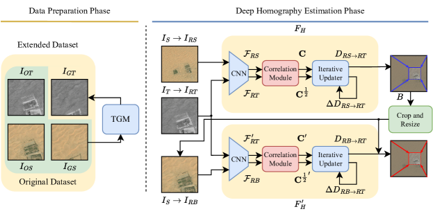
Figure 2: STHN Framework Overview: For the data preparation phase, TGM produces synthetic thermal images from unpaired satellite images, augmenting the dataset. The deep homography estimation phase employs an iterative update approach, using $F_{H}$ to predict the displacement $D_{RS\rightarrow RT}$ between thermal images and satellite maps. For refinement, the framework crops and resizes the selected region $B$, utilizing $F^{\prime}_{H}$ to fine-tune the four-corner displacement prediction for enhanced accuracy.

III Methodology

Our STHN framework, shown in Fig. 2, has three main components: Thermal Generative Module (TGM), coarse alignment module, and refinement module.

III-A Thermal Generative Module

Due to limited satellite-thermal image pairs, we employ the Thermal Generative Module (TGM) introduced by [11] to enhance our training dataset with synthetic thermal images derived from satellite images. In the data preparation phase, we denote $I_{OS}$ and $I_{OT}$ as the pair of satellite and thermal images from the original dataset, and $I_{GS}$ as the satellite images without paired thermal images. We train TGM with the input $I_{OS}$ and target output $I_{OT}$ (detailed in [11]). After training TGM, we generate synthetic thermal images $I_{GT}$ using TGM and $I_{GS}$, and combine $I_{OS}$ and $I_{OT}$ to build an extended satellite-thermal dataset. We denote the quantity of actual thermal images as $N_{T}$ and those generated as $N_{G}$. We restrict our sampling from the generated dataset per epoch to $N_{T}$ instances to mitigate bias towards the generated dataset, given that $N_{T}\ll N_{G}$.

III-B Coarse-to-fine Iterative Homography Estimation

Our coarse-to-fine strategy is divided into two stages: Coarse alignment and refinement.

III-B1 Coarse Alignment Stage

We denote $W_{S}$ as the width of input square satellite images $I_{S}$ and $W_{T}$ as that of input square thermal images $I_{T}$. For pre-processing, we resize $I_{S}$ and $I_{T}$ to $I_{RS}$ and $I_{RT}$ at the side length of $W_{R}$, and the resize ratios of $I_{RS}$ is $\alpha=W_{S}/W_{R}$. The homography estimation process is

$$D_{RS\rightarrow RT}=F_{H}(I_{RS},I_{RT}),$$ (1)

where $D_{RS\rightarrow RT}\in\mathbb{R}^{2\times 4}$ is the displacement from the four corners of $I_{RS}$ to those of $I_{RT}$ and $F_{H}$ is the homograph estimation model. $F_{H}$ follows iterative estimation paradigm [12], which consists of three modules: A Convolutional Neural Network (CNN) [25] feature extractor outputs the feature map $\mathcal{F}_{RS},\mathcal{F}_{RT}\in\mathbb{R}^{C\times\frac{W_{R}}{4}\times\frac{W_{R}}{4}}$ ($C$ is the channel of feature map and is set to $256$), a correlation module outputs correlation volumes [34] $\mathbf{C}$ ($\frac{W_{R}}{4}\times\frac{W_{R}}{4}\times\frac{W_{R}}{4}\times\frac{W_{R}}{4}$) and $\mathbf{C}^{\frac{1}{2}}$ ($\frac{W_{R}}{4}\times\frac{W_{R}}{4}\times\frac{W_{R}}{8}\times\frac{W_{R}}{8}$), and an iterative homography estimator provides the update of the displacement $\Delta D_{RS\rightarrow RT}$. At iteration $k$, $D_{RS\rightarrow RT}$ is updated as

$$D_{k+1,RS\rightarrow RT}=D_{k,RS\rightarrow RT}+\Delta D_{k,RS\rightarrow RT}.$$ (2)

Since the images are resized during pre-processing, the displacement of the coarse alignment stage on the scale of $I_{S}$ is $D^{\prime}_{S\rightarrow T}=\alpha D_{RS\rightarrow RT}$. For the loss function, we minimize the L1 distance between the predicted displacements $D_{k,RS\rightarrow RT}$ and ground truth ones $D^{gt}_{k,RS\rightarrow RT}$ with exponential decay as

$$\mathcal{L_{\textrm{coarse}}}=\sum_{k=0}^{K_{1}-1}\gamma^{K_{1}-k-1}\|D_{k,RS\rightarrow RT}-D^{gt}_{k,RS\rightarrow RT}\|_{1},$$ (3)

where $K_{1}$ is the number of updates in the coarse alignment. $D_{RS\rightarrow RT}=D_{K_{1},RS\rightarrow RT}$. The decay factor $\gamma$ is $0.85$.

III-B2 Refinement Stage

We create a bounding box $B$ that bounds the corners of thermal images warped by $D^{\prime}_{S\rightarrow T}$. We denote $D_{S\rightarrow B}\in\mathbb{R}^{2\times 4}$ as the four-corner displacement from $I_{S}$ to $B$. We crop out the region of $B$ to get $I_{B}$ at the side length of $W_{B}$ and resize it to $I_{RB}$ at the side length of $W_{R}$. The resize ratio is $\delta=W_{B}/W_{R}$. The refinement process is

$$D_{RB\rightarrow RT}=F^{\prime}_{H}(I_{RB},I_{RT}),$$ (4)

where $F^{\prime}_{H}$ has the same structure as $F_{H}$ with iterative updates (Equation 2) but does not share weights and $D_{RB\rightarrow RT}\in\mathbb{R}^{2\times 4}$ are four-corner displacement from $I_{RB}$ to $I_{RT}$. We set $\kappa=\delta/\alpha$ and the loss function is

$$\mathcal{L_{\textrm{fine}}}=\sum_{k=0}^{K_{2}-1}\gamma^{K_{2}-k-1}\kappa\|D_{k,RB\rightarrow RT}-D^{gt}_{k,RB\rightarrow RT}\|_{1},$$ (5)

where $D_{k,RB\rightarrow RT}$ and $D^{gt}_{k,RB\rightarrow RT}$ are predicted and ground truth displacements, and $K_{2}$ is the number of updates in the refinement. $\kappa$ maps the displacement from the scale of $I_{RB}$ to the scale of $I_{RS}$, aligning with $\mathcal{L_{\textrm{coarse}}}$. The displacement of the refinement stage on the scale of $I_{S}$ is $D^{\prime\prime}_{S\rightarrow T}=\delta D_{RB\rightarrow RT}$. Combining the two stages’ results, we get the final displacement

$$D_{S\rightarrow T}=D_{S\rightarrow B}+D^{\prime\prime}_{S\rightarrow T}.$$ (6)

With $D_{S\rightarrow T}$, we use Direct Linear Transformation (DLT) [35] to solve the homography transformation matrix $H$. The transformed center coordinate $(x_{c},y_{c})$ is calculated as

$$\left(x_{c},y_{c},1\right)^{\top}=H\times\left(\frac{W_{S}}{2},\frac{W_{S}}{2},1\right)^{\top},$$ (7)

which is used for geo-localization. The total loss function is

$$\mathcal{L}=\mathcal{L_{\textrm{coarse}}}+\mathcal{L_{\textrm{fine}}}.$$ (8)

III-C Two-stage Training Strategy

For training the two-stage model, we first train the coarse alignment module from scratch, and then we attach the refinement module to the end of the coarse alignment module and jointly fine-tune the two modules. We discovered that augmenting the bounding box $B$ is crucial for effectively fine-tuning the refinement module. This requirement arises because the refinement module always tends to make no or only minor adjustments if the coarse alignment already performs well on training and validation sets. Furthermore, we observed that merely fixedly expanding the cropped boxes without random shifting and enlargement does not enhance performance. To boost the refinement module’s effectiveness, we augment $B$ by shifting the center coordinates $(x_{B},y_{B})$ by $(\Delta p_{1},\Delta p_{2})$ and expanding the width $W_{B}$ by $2\Delta p_{3}$ during training. During the evaluation phase, we consistently expand $W_{B}$ by $\Delta p_{4}$ to mitigate the potential offset error of the coarse alignment.

IV Experimental Setup

In this section, we outline the experimental settings, covering the dataset (Section IV-A), evaluation metrics (Section IV-B), and implementation details (Section IV-C).

IV-A Dataset

For training and evaluation, our study utilizes the Boson-nighttime [11] real-world dataset which contains $10,256$ train pairs, $13,011$ validation pairs, and $26,568$ test pairs of coupled satellite RGB and nadir-view thermal imagery. We have expanded the dataset by augmenting the collection of satellite images without corresponding thermal images from $79,950$ to $163,344$ images, covering the area of $215.78~{}$\mathrm{k}\mathrm{m}$^{2}$. This enhancement focuses on the desert and farm areas near the original dataset’s sampling region, thereby incorporating a broader spectrum of geographical patterns. Additionally, the test region is then excluded from the generated data to ensure a robust evaluation of generalization performance. The thermal images in the dataset are captured between 9:00 PM and 4:00 AM, and they are aligned with an approx. spatial resolution of $1~{}$\mathrm{m}\mathrm{/}\mathrm{p}\mathrm{x}$$. The thermal images are cropped to $W_{T}\times W_{T}$ pixels ($\mathrm{p}\mathrm{x}$), where $W_{T}=512$. The satellite images are cropped to $W_{S}\times W_{S}$, where $W_{S}$ can be $512$, $1024$, or $1536$. Fig. 3 shows the ground truth overlap between thermal images and satellite images with different $W_{S}$. For $W_{S}=1024$ and $1536$, the overlap ratios are $25\%$ and $11\%$, if the thermal images are fully within the satellite region.

Satellite ($W_{S}=512$)

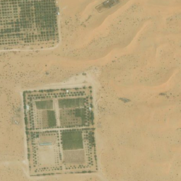
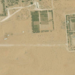
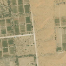
Thermal

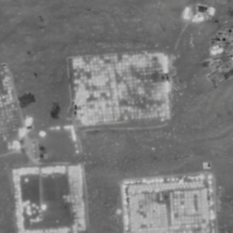
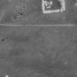
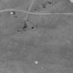
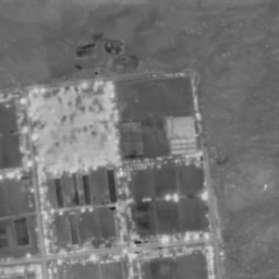
$W_{S}=512$

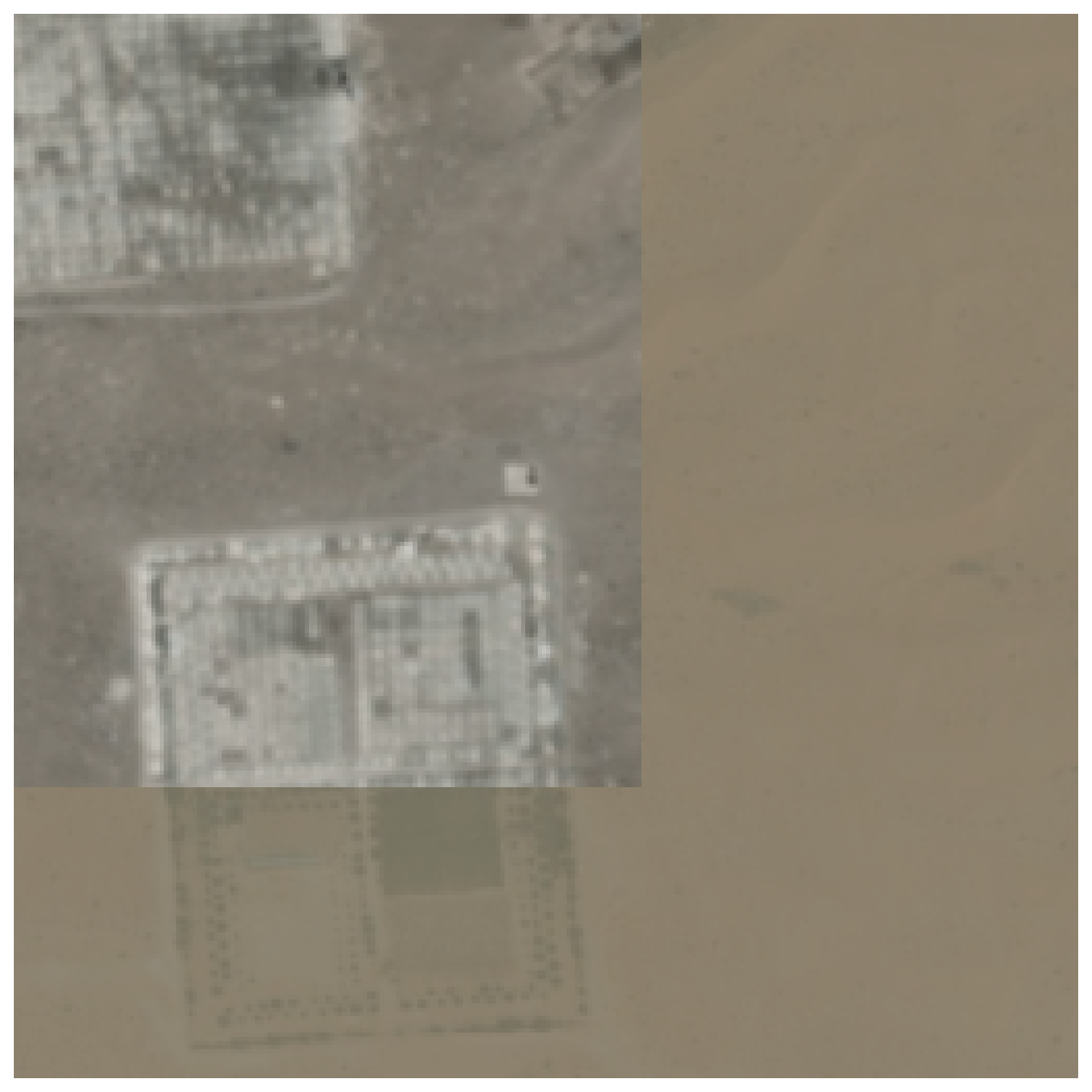
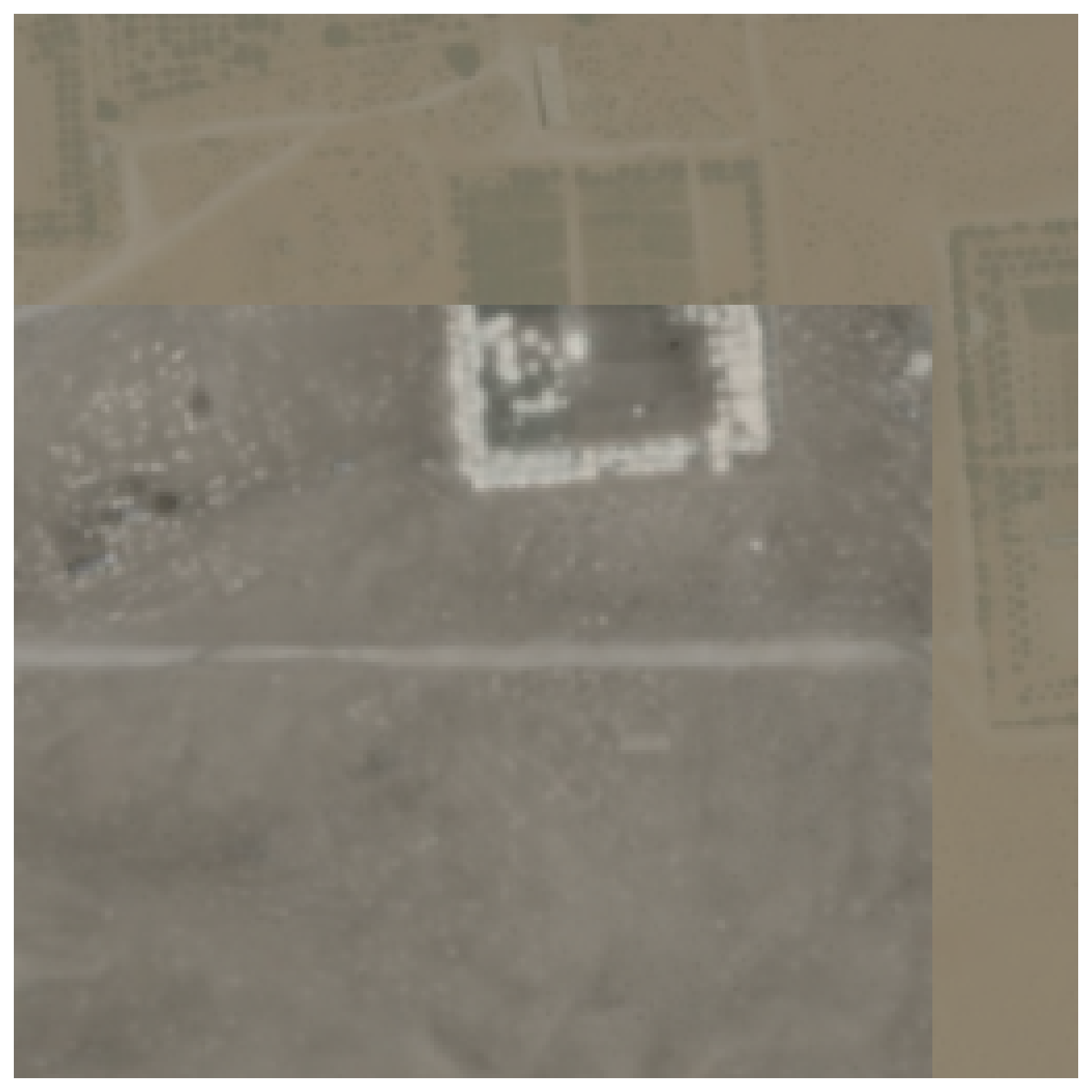
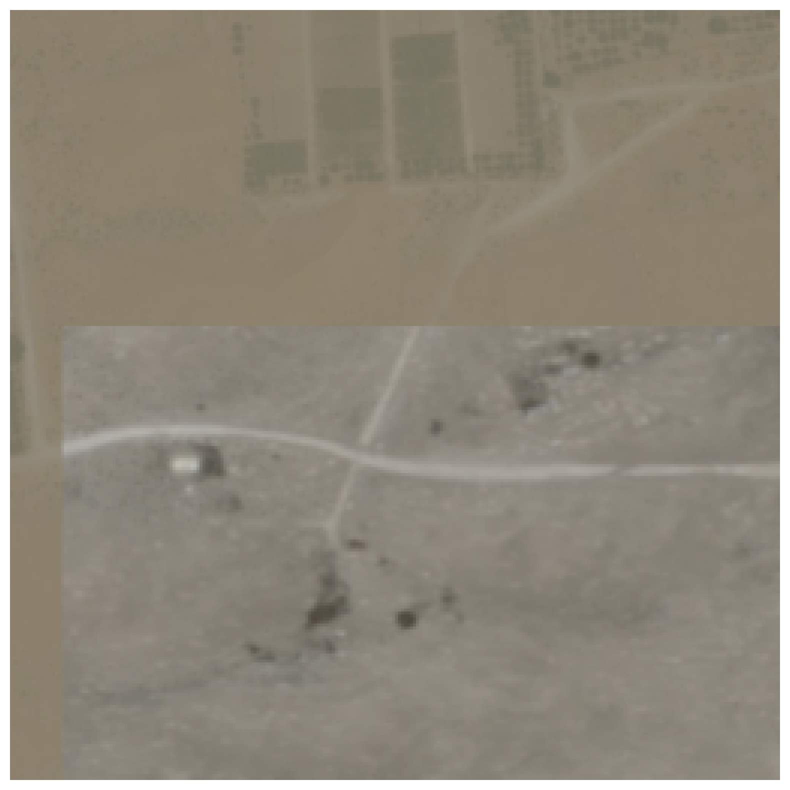
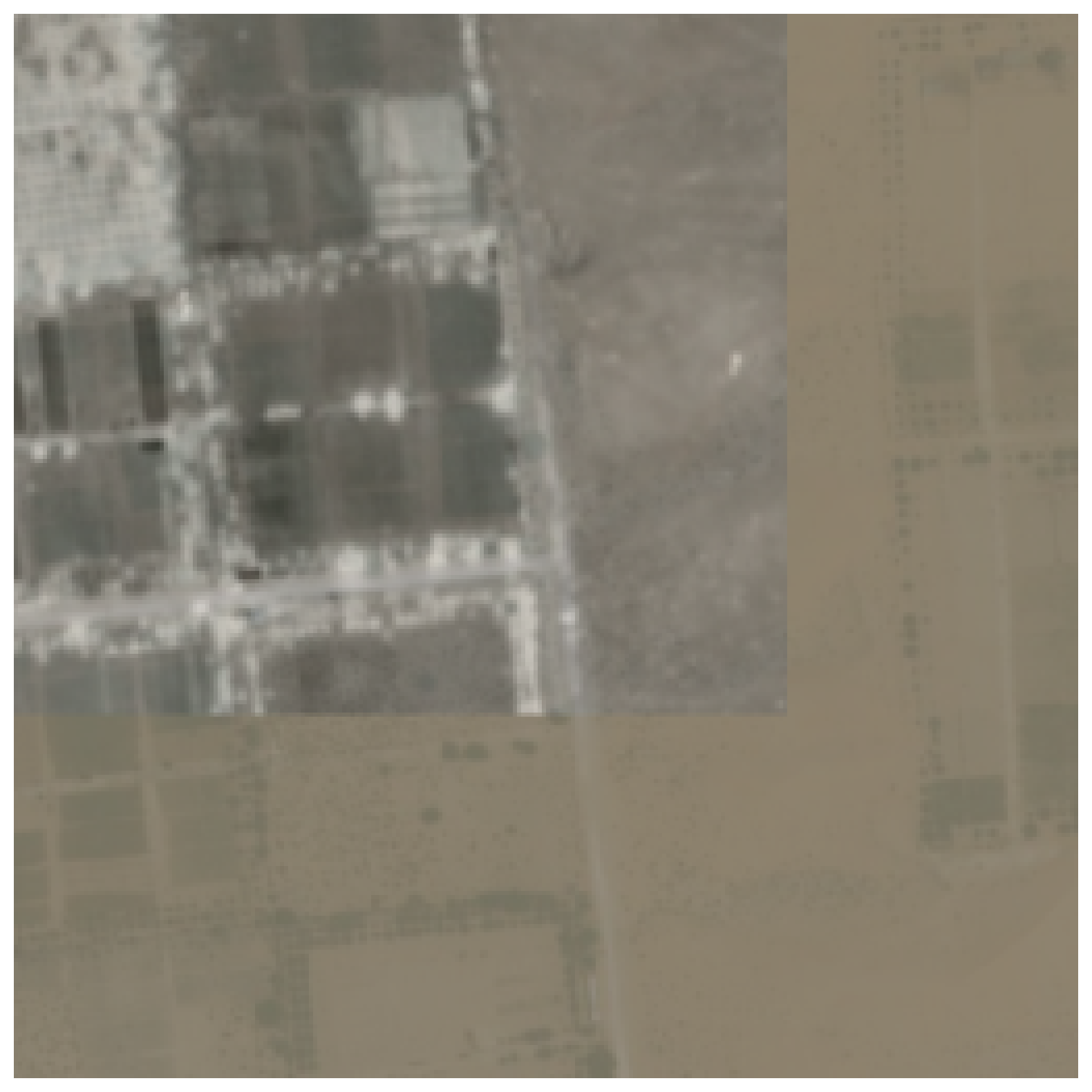
$W_{S}=1024$

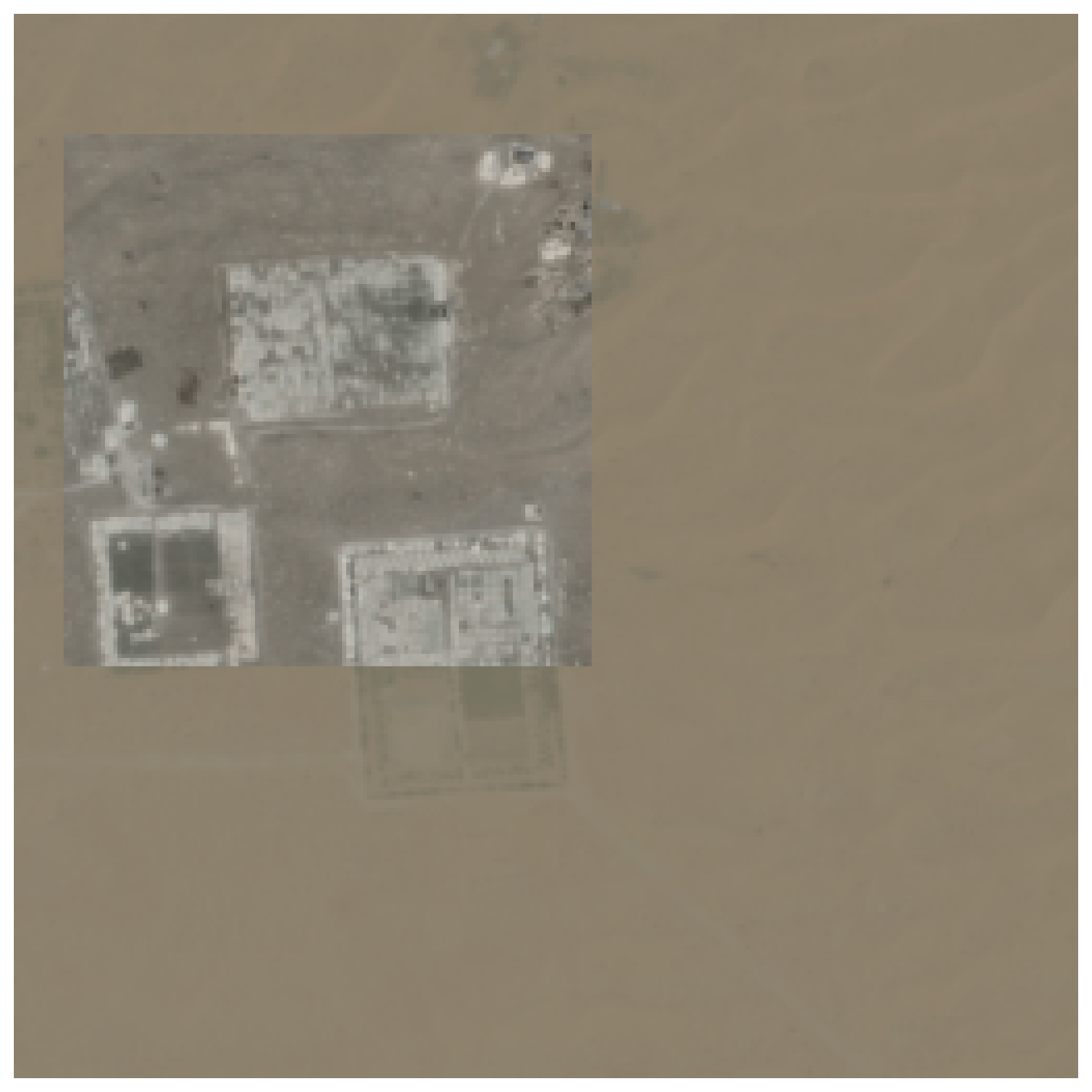
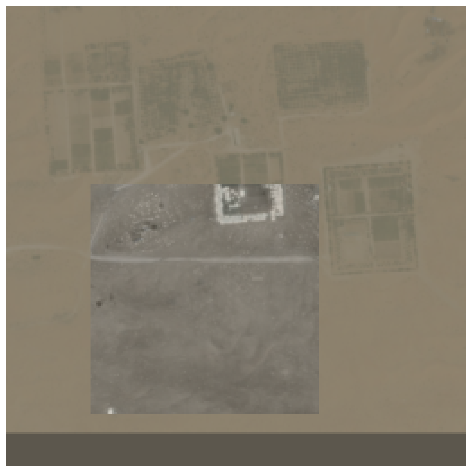
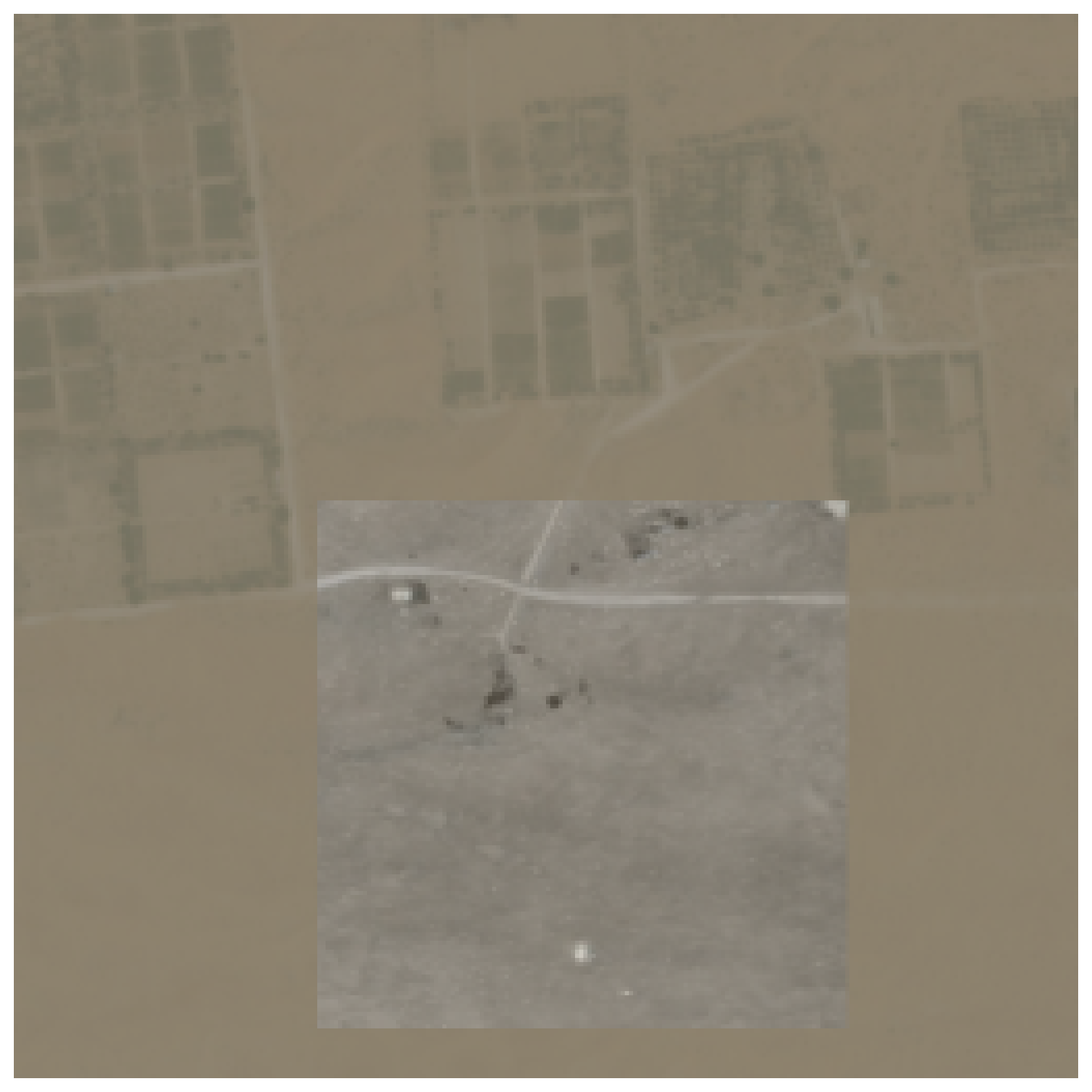
$W_{S}=1536$

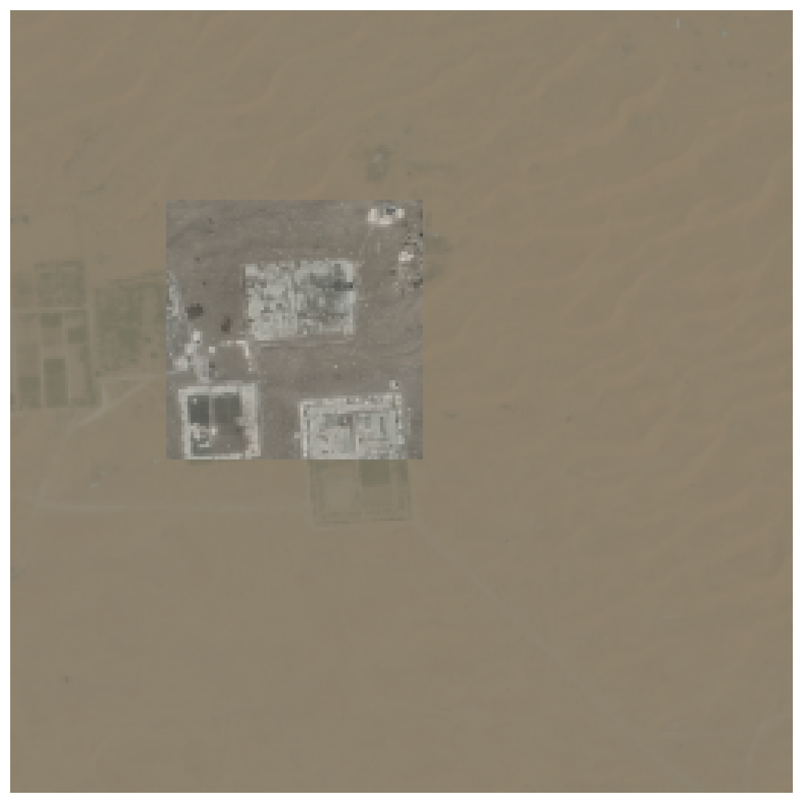
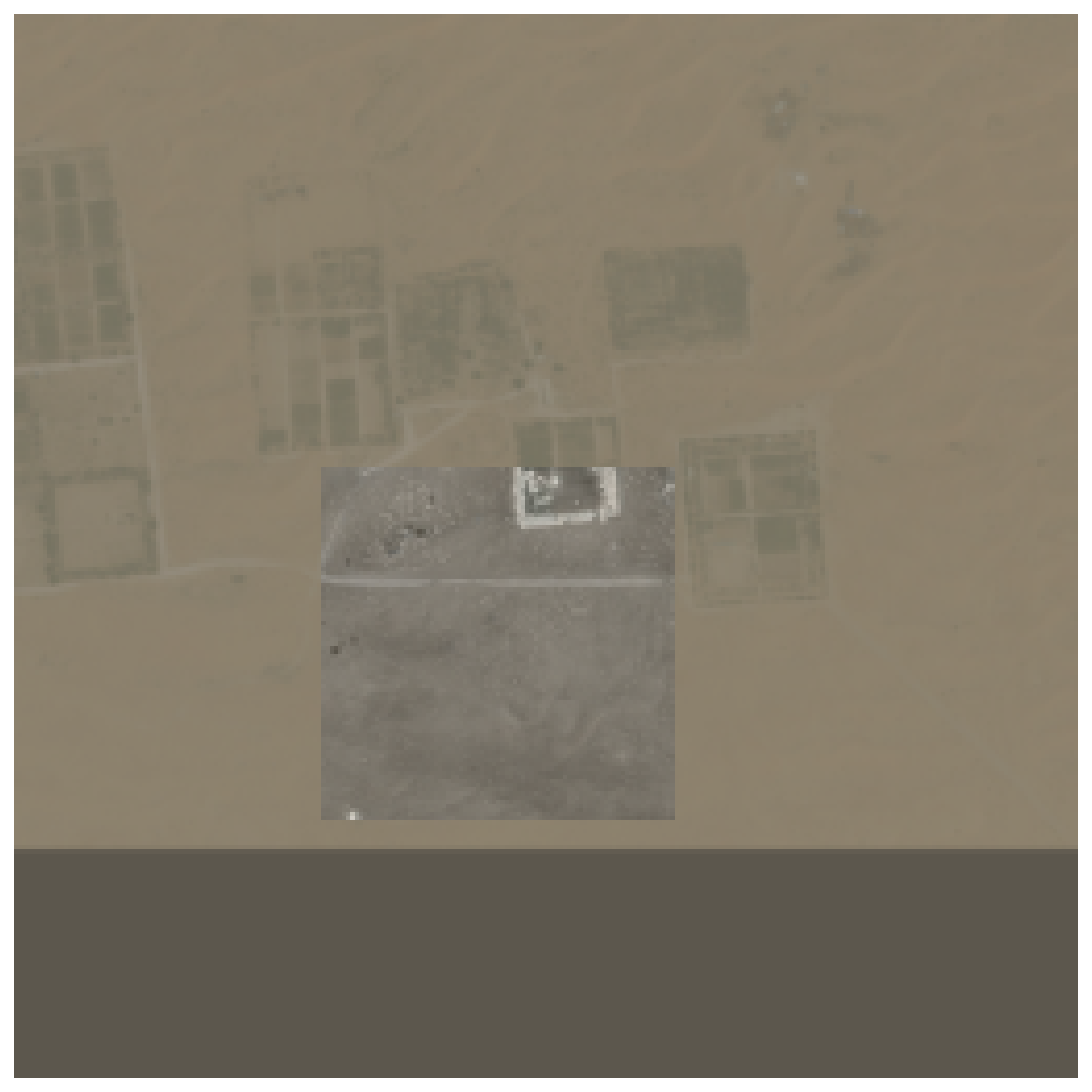
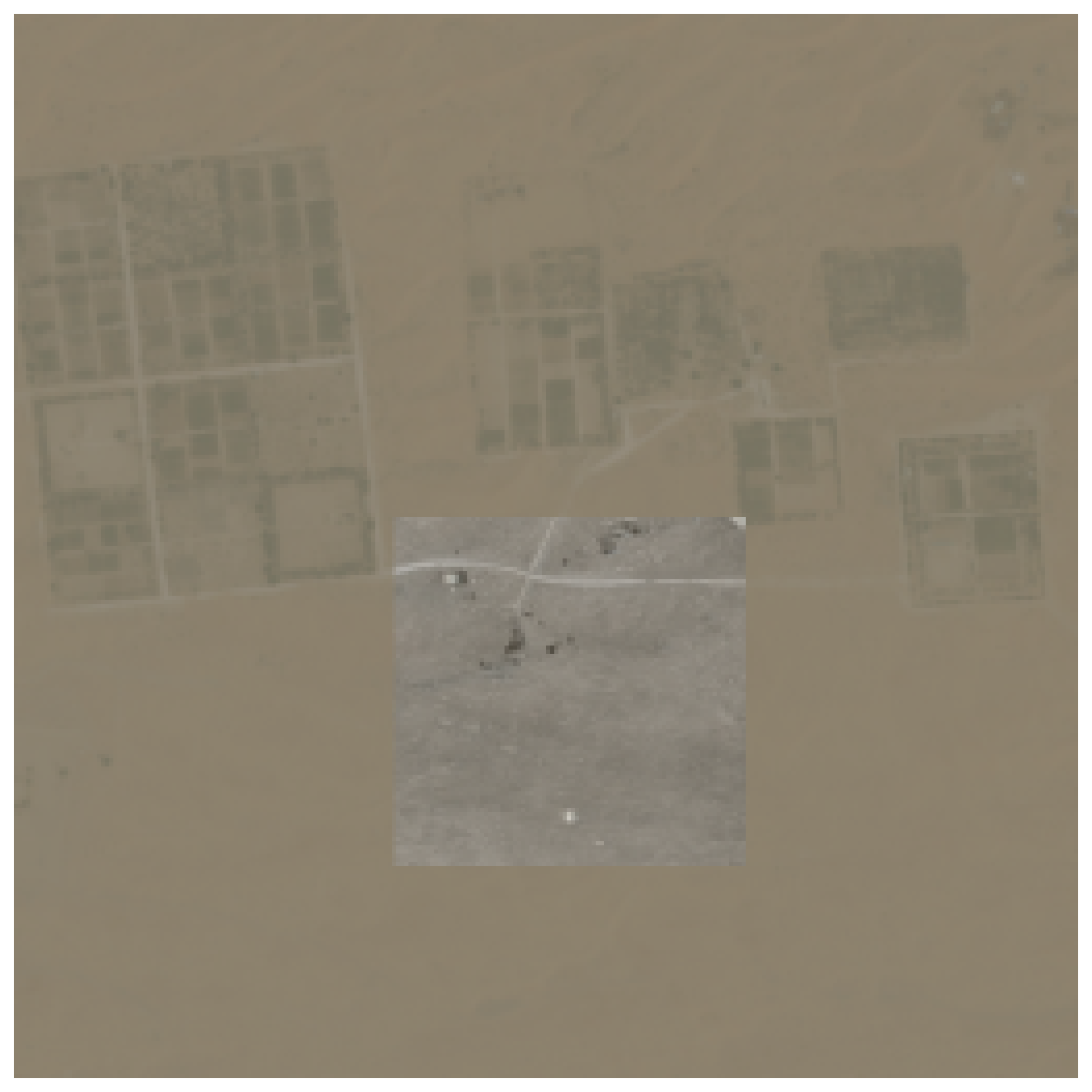
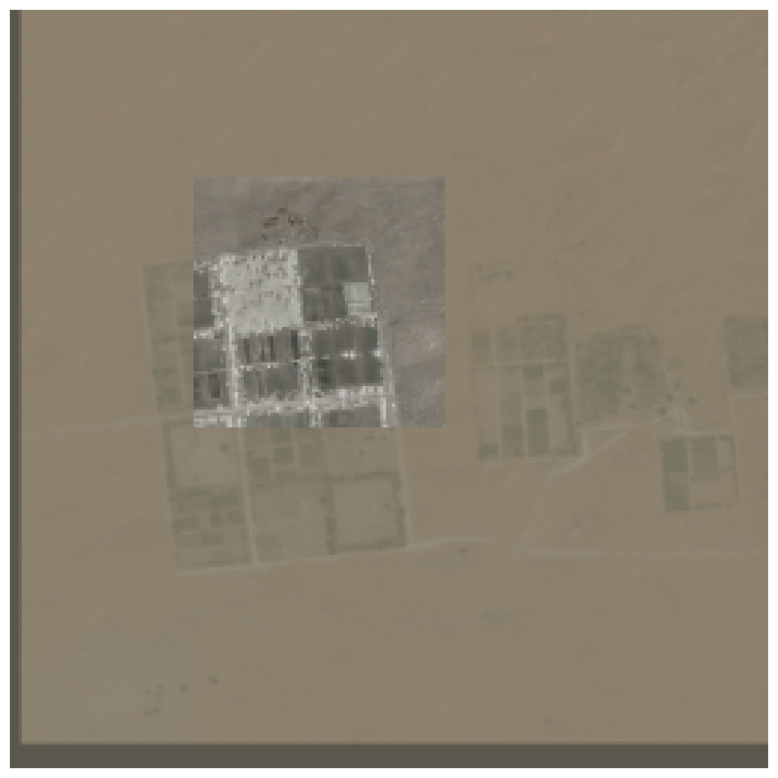
Figure 3: The example images of Boson-nighttime dataset. The $1^{\textrm{st}}$ row and $2^{\text{nd}}$ row are input satellite and thermal images. The $3^{\text{rd}}$-$5^{\text{th}}$ rows are the ground truth overlap between satellite and thermal images with different $W_{S}$.

IV-B Metrics

We deploy two accuracy metrics in our evaluation: Mean Average Corner Error (MACE) and Center Error (CE). MACE, extensively adopted in previous studies on deep homography estimation [13, 12, 17], measures the mean value of the average distances between the four corners of estimated and ground truth image alignments. Conversely, CE measures the mean value of the distances between the center points of predicted thermal image displacements and ground truth ones, thereby measuring geo-localization accuracy.

In our experimental analysis, the maximum spatial distance between the center points of input thermal and satellite images $D_{C}$ emerges as a critical factor influencing estimation performance. Intuitively, a larger $D_{C}$ implies a greater translation from the center required for the four-corner displacement, which in turn becomes more challenging to predict accurately. To validate the robustness of our method, we cautiously ablate results across a spectrum of $D_{C}$, demonstrating our approach’s capability to maintain reliable performance under varying degrees of challenging translations.

IV-C Implementation Details

For pre-processing, the resize side length $W_{R}$ is $256~{}$\mathrm{p}\mathrm{x}$$. The training iteration numbers of the coarse alignment and refinement modules are $200000$ with a batch size of $16$. The AdamW optimizer [36] is employed for model training, utilizing a linear learning rate decay scheduler with warmup with the peak learning rate at $1\mathrm{e}{-4}$. The numbers of iterative updates $K_{1}$ and $K_{2}$ are both set to $6$. Depending on the setting, the correlation module’s level is $2$ (for $W_{S}=512$) or $4$ (for $W_{S}=1024,1536$) with a search radius of $4$. For bounding box augmentation, $\Delta p_{1},\Delta p_{2}$ is set to vary between $(-64,64)$, $\Delta p_{3}$ is set within $[0,64)$, and $\Delta p_{4}$ is $64$ by parameter tuning. Our models are developed using PyTorch. The inference speed is measured with one NVIDIA RTX-2080-Ti GPU.

V Results

TABLE I: Comparison of test MACE (m) between different homography estimation methods across different $D_{C}$. ”Identity” indicates the error if no homography estimation is applied. If not specified, the methods are evaluated with $W_{S}=512$.

Methods	$D_{C}=50~{}$\mathrm{m}$$	$D_{C}=64~{}$\mathrm{m}$$	$D_{C}=128~{}$\mathrm{m}$$	$D_{C}=256~{}$\mathrm{m}$$	$D_{C}=512~{}$\mathrm{m}$$	Failure Rate
Traditional Keypoint Matching Methods
Identity	35.63	39.08	85.63	170.94	334.68	-
SIFT [37] + RANSAC [38]	442.20	654.77	547.29	529.63	1650.46	99.6%
SIFT [37] + MAGSAC++ [39]	512.60	438.54	529.46	561.64	693.03	99.7%
ORB [40] + RANSAC [38]	720.80	733.69	733.94	4614.84	975.83	82.6%
ORB [40] + MAGSAC++ [39]	784.12	558.51	564.63	524.99	573.72	82.9%
BRISK [41] + RANSAC [38]	503.25	771.21	665.94	974.80	591.17	95.5%
BRISK [41] + MAGSAC++ [39]	536.52	487.95	722.76	1948.99	568.24	95.6%
Deep Homography Estimation Methods
DHN [13]	16.78	20.43	77.68	197.27	457.23	0%
LocalTrans [16]	33.31	37.29	86.04	166.52	338.21	0%
IHN [12]	5.91	7.81	51.74	190.93	367.24	0%
Ours ($W_{S}=512$)	4.24	4.93	14.97	142.71	347.50	0%
Ours ($W_{S}=1024$)	4.92	5.31	6.03	9.22	86.74	0%
Ours ($W_{S}=1536$)	6.50	7.04	7.27	16.78	16.42	0%
Ours ($W_{S}=1536$ + two stages)	7.51	7.20	7.51	14.99	12.70	0%

TABLE II: Comparison between different image-based matching methods and our homography estimation methods when $D_{C}=512$\mathrm{m}$$.

Methods	Test CE ($\mathrm{m}$)	Latency ($\mathrm{m}\mathrm{s}$)
Image-based Matching Methods
AnyLoc-VLAD-DINOv2 [29]	258.21	352404.03
STGL-NetVLAD-ResNet50 [11, 42]	89.31	7180.0
STGL-GeM-ResNet50 [11, 43]	13.52	4918.9
Deep Homography Estimation Methods
Ours ($W_{S}=1536$)	15.90	35.2
Ours ($W_{S}=1536$ + two stages)	12.12	63.9

In this section, we present both quantitative and qualitative analysis in Boson-nighttime [11]. For a fair comparison, we ensure the same data and pipeline consistency steps for training and evaluating across all methods. Initially, in Section V-A and V-B, we establish a baseline by assuming that thermal images are aligned to the north, facilitated by an onboard compass and a gimbal-equipped thermal camera, with our focus primarily on translation error. Subsequently, in Section V-C, we broaden our analysis to encompass geometric noises such as rotation, resizing, and perspective transformation noises.

V-A Comparison with Baselines

In the results detailed in Table I, we initiate the analysis by evaluating the efficacy of traditional keypoint matching methods, such as SIFT [37], ORB [40], and BRISK [41], integrated with outlier rejection methods like RANSAC [38] and MAGSAC++ [39]. These traditional methods demonstrate a significantly high MACE alongside substantial failure rates (calculated by instances where the number of matching keypoints $\leq 10$). This underlines the challenges inherent in complex satellite-thermal alignment.

Subsequently, our analysis compares our methods with various deep homography estimation frameworks, including DHN [13], LocalTrans [16], and IHN [12] (State-of-the-art method in real-time applications). These baselines are trained on the Boson-nighttime dataset with one stage for comparison. The results show the superior performance of our methods for satellite-thermal alignment and geo-localization. A notable observation from the data is the differential performance preferences across varying $D_{C}$ distances: for $D_{C}=50~{}$\mathrm{m}$$ and $D_{C}=64~{}$\mathrm{m}$$, the optimal $W_{S}$ is $512$, while for mid-range distances of $D_{C}=128~{}$\mathrm{m}$$ and $D_{C}=256~{}$\mathrm{m}$$, using $W_{S}=1024$ leads to the best results. Additionally, for the longest distance of $D_{C}=512~{}$\mathrm{m}$$, our novel two-stage method with $W_{S}=1536$ emerges as the most effective strategy. The findings indicate that for cases where $D_{C}\leq 256~{}$\mathrm{m}$$, employing our one-stage method combined with a carefully chosen $W_{S}$ emerges as the most effective strategy. We offer further explanation of the correlation between $W_{S}$ and $D_{C}$ in Section V-B.

We find that our two-stage method fails to enhance performance for distances $D_{C}=50~{}$\mathrm{m}$$, $64~{}$\mathrm{m}$$, and $128~{}$\mathrm{m}$$, instead leading to a decline in accuracy. Upon examining the visualized outcomes, we observe that for smaller distances ($D_{C}\leq 128~{}$\mathrm{m}$$), the initial coarse alignment is sufficiently accurate, making the refinement module’s excessive iterative updates introduce noise into the final predictions, thereby degrading performances. Nevertheless, our two-stage approach maintains an overall MACE of less than $15~{}$\mathrm{m}$$ across all considered $D_{C}$ values, establishing robust baselines for this task. Notably, for achieving precise geo-localization at a distance of $D_{C}=512~{}$\mathrm{m}$$, this two-stage strategy demonstrates the best performance, underscoring our method’s effectiveness for large-scale search regions.

We also compare with image-based solutions  (AnyLoc [29] and STGL [11]) on accuracy and latency aspects in Table II. The latency of image-based matching methods is calculated by $t_{e}\times(N_{S}+1)+t_{m}$, where $t_{e}$ is feature extraction time per image, and $N_{S}=841$ is the number of database images centered within a $1024\times 1024$ area (while the complete images cover a $1536\times 1536$ area) with a sampling stride of $35$ px following [11]. $t_{m}$ is the matching time per query. For AnyLoc, we directly apply the original DINOv2 [44] weights and fit the VLAD [45] parameters using our training data. We have observed a significant performance decline in AnyLoc, likely due to the domain gap between satellite and thermal imagery. STGL with GeM yields high accuracy but still suffers from high latency. Our methods exhibit significant enhancements in both accuracy and latency compared to these existing image-based matching techniques. Notably, our one-stage and two-stage methods achieve latency reductions to just $7.2\%$ and $13.0\%$ of the latency of STGL-GeM-ResNet50.

V-B Ablation Study

In this study (Figs. 4-6), we focus on the following questions

• How does the incorporation of TGM affect the accuracy of homography estimation across varying $D_{C}$?

• Is the coarse alignment effective in achieving satisfactory localization accuracy for large $D_{C}$?

• Is the bounding box augmentation effective for fine-tuning the refinement module?

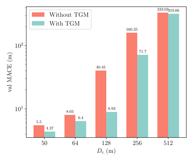
Figure 4: Effectiveness of TGM in deep homography estimation across different $D_{C}$ when $W_{S}=512$. Validation MACE (Val MACE) is plotted on a log scale.

V-B1 Effectiveness of TGM

Fig. 4 demonstrates the effectiveness of TGM in improving deep homography estimation over different spatial distances between centers ($D_{C}$) on the validation set. It showcases TGM’s ability to enhance estimation accuracy by generating synthetic thermal images for satellite imagery that lacks paired thermal data. This consistent enhancement in image-based matching [11] and deep homography estimation for satellite-thermal matching suggests TGM’s potential applicability in additional computer vision tasks that do not have direct thermal imaging counterparts.

V-B2 Coarse alignment

Fig. 5 illustrates the correlation between validation MACE and $W_{S}$ across various $D_{C}$. The figure shows that as $W_{S}$ increases, the validation MACE for smaller translation distances ($D_{C}=50~{}$\mathrm{m}$$ and $64~{}$\mathrm{m}$$) slightly increases, suggesting a deterioration in alignment accuracy. In contrast, for larger translation distances ($D_{C}=128~{}$\mathrm{m}$$, $256~{}$\mathrm{m}$$, $512~{}$\mathrm{m}$$), the validation MACE decreases, indicating improved alignment accuracy. The intuition is that an increase in $W_{S}$, without a corresponding adjustment in $W_{R}$, leads to a higher pixel-per-meter (ppm) ratio after image resizing. This increment in ppm ratio can negatively affect the alignment accuracy. Conversely, a larger $W_{S}$ enhances alignment accuracy for greater translation ($D_{C}$), especially for $W_{S}=1536$ and $D_{C}=512~{}$\mathrm{m}$$. In these cases, a larger $W_{S}$ ensures the full coverage of the thermal image, which is crucial for accurately calculating correlation volumes $\mathbf{C}$.

V-B3 Effectiveness of Bounding Box Augmentation

We present a qualitative comparison in Fig. 6 to demonstrate the impact of fine-tuning with and without bounding box augmentation (bbox aug). Given that bounding box augmentation requires an expansion of the bounding box (bbox exp) during the evaluation phase, we also include results featuring solely bbox exp without bbox aug to ablate the effects. The findings illustrate that in the absence of augmentation, the refinement module tends to make only minimal adjustments when not trained with bbox exp. On the other hand, if we train the refinement module with only bbox exp, it always tends to reduce the size of the predicted box towards the center, rather than correctly repositioning it. However, the incorporation of augmentation addresses these limitations by augmenting the width and the center coordinates of the region.

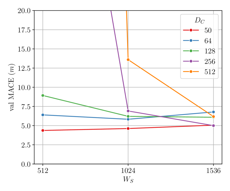
Figure 5: Coarse alignment under large-scale ($W_{S}=1536$), median-scale ($W_{S}=1024$), small-scale ($W_{S}=512$) satellite images with TGM.

V-C Robustness Evaluation and Visualization

In an ideal setting, the UAV onboard compass and gimbal camera would supply precise data, enabling the accurate alignment of images to the north. However, it is crucial for our algorithm to demonstrate tolerance towards certain rotation and perspective transformation inaccuracies during active flights. Additionally, understanding how our algorithm performs when there is a change in flight altitude—which results in a change of the thermal image’s coverage area, denoted as resizing noise—is essential. To assess the algorithm’s robustness under these conditions, we perform experiments that introduce specific rotation, resizing, and perspective transformation noises. For rotation disturbances, the thermal images undergo random rotations of $5^{\circ}$, $10^{\circ}$, or $30^{\circ}$. For resizing disturbances, the images are randomly scaled by a factor of $1+\Delta r$, with $\Delta r$ being either $\pm 0.1$, $\pm 0.2$, or $\pm 0.3$. Regarding perspective transformation disturbances, we randomly adjust the four corners of $512\times 512$ thermal images by $8~{}$\mathrm{p}\mathrm{x}$$, $16~{}$\mathrm{p}\mathrm{x}$$, or $32~{}$\mathrm{p}\mathrm{x}$$.

In Table III, we evaluate the robustness of our one-stage and two-stage strategies against a variety of geometric noise conditions with $D_{C}=512~{}$\mathrm{m}$$ and $W_{S}=1536$. The analysis indicates a significant decrease in performance for the one-stage method under these conditions, in contrast to the two-stage strategy, which demonstrates a notable robustness against geometric perturbations. Specifically, the two-stage strategy effectively maintains test MACE below $24~{}$\mathrm{m}$$ and test CE below $22~{}$\mathrm{m}$$ in most scenarios, with notable exceptions being in instances of $30^{\circ}$ rotation noise and resizing noise with a factor of $0.3$. While incremental perspective transformations have minimal impact on accuracy, large rotation and resizing noise can significantly degrade performance. This suggests the tolerance of our strategies to varying types of noise. Overall, the results validate the robustness of our methodologies against a spectrum of geometric noises, especially underscoring the two-stage strategy’s superior effectiveness and reliability in mitigating the negative effects of these disturbances. Fig. 7 further illustrates this point by showcasing visual comparisons between the failure instances of the one-stage method and the success cases of the two-stage method, thereby demonstrating the latter’s improved robustness.

w/o bbox aug

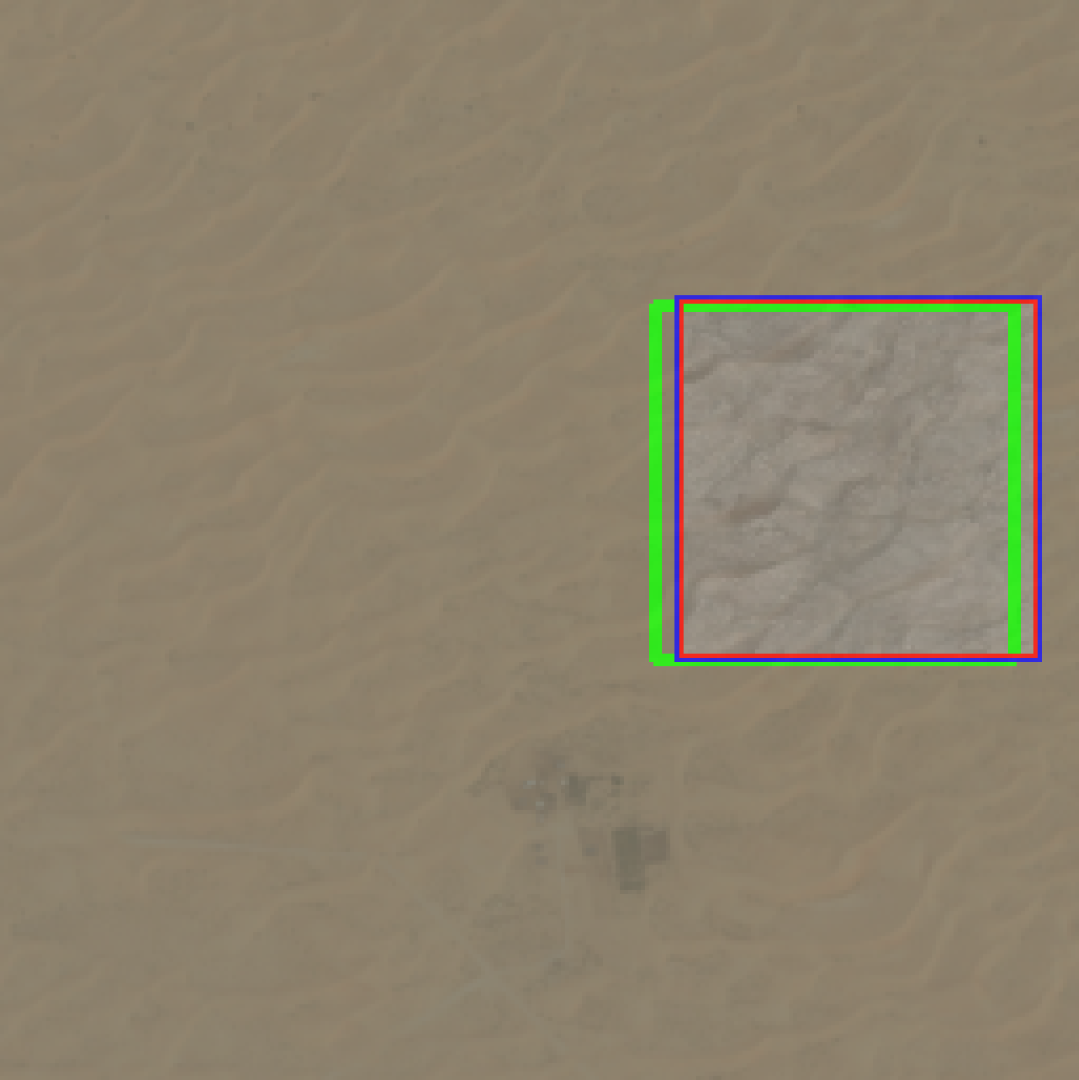
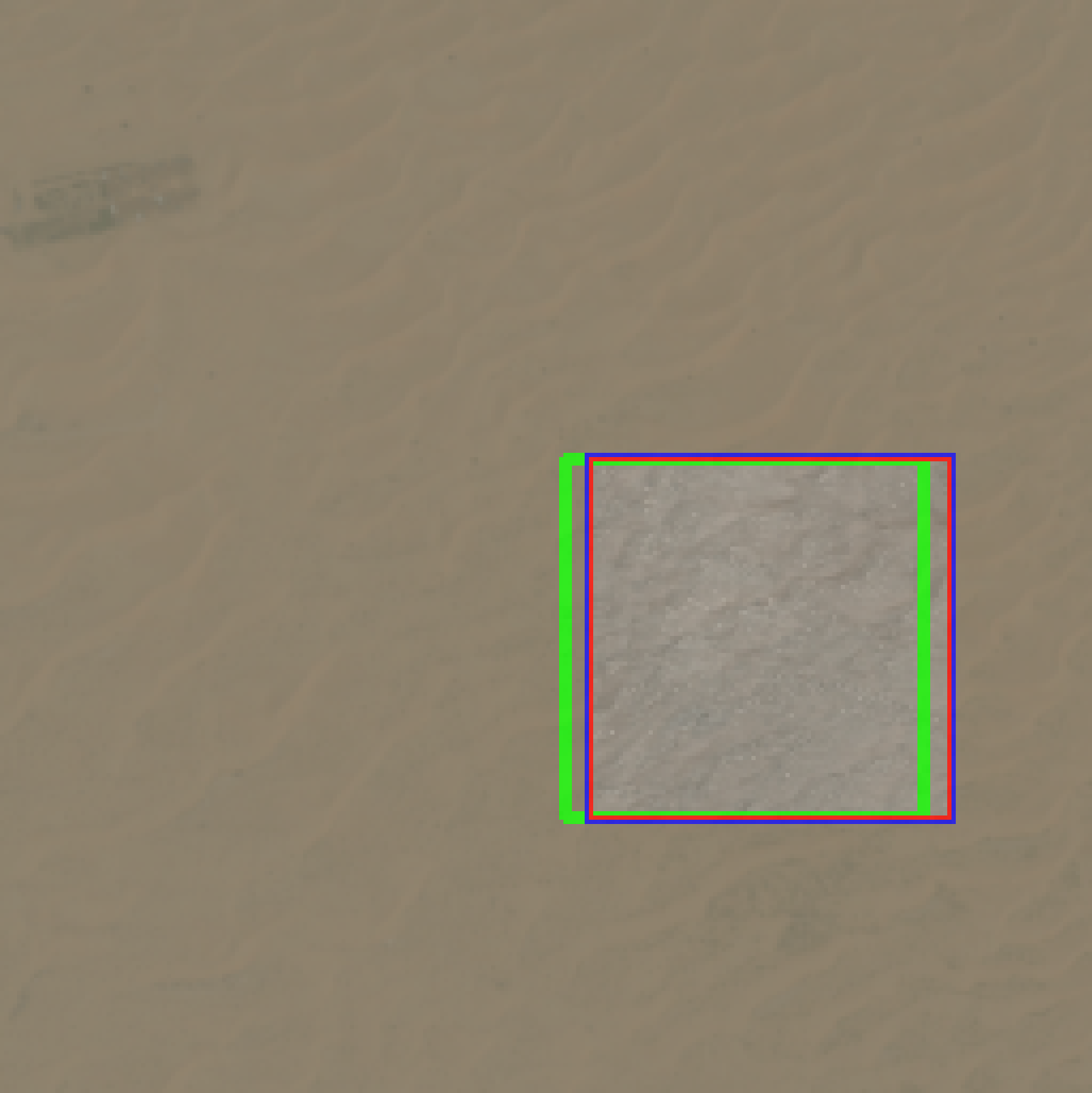
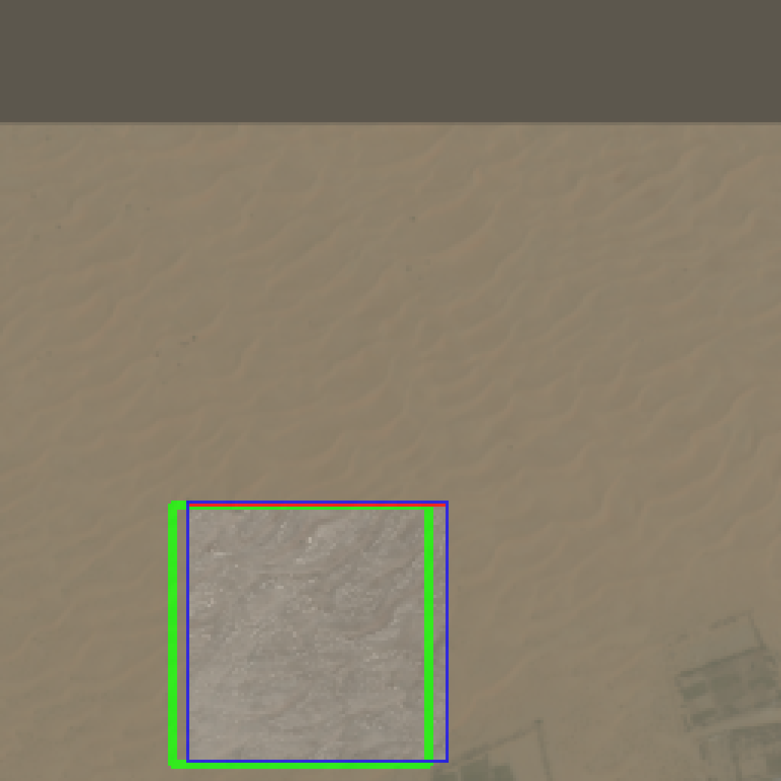
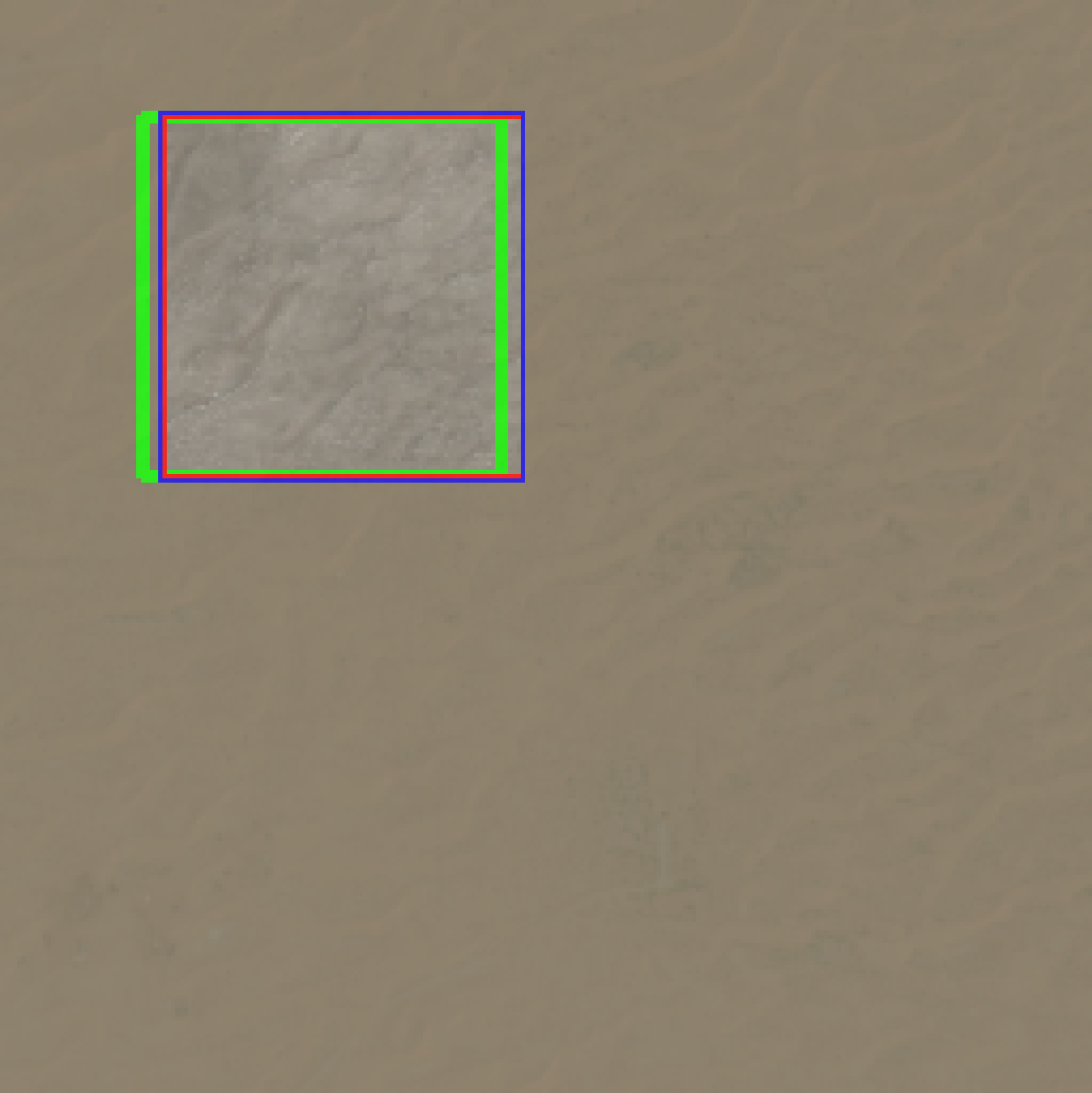
w/ bbox exp

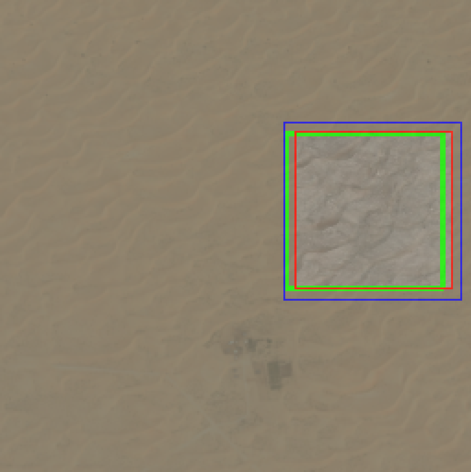
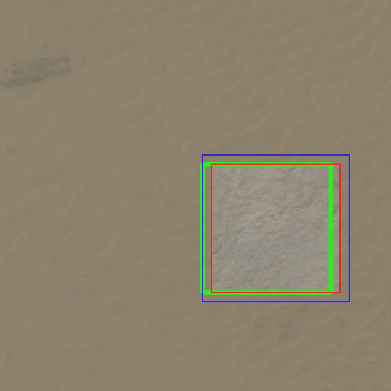
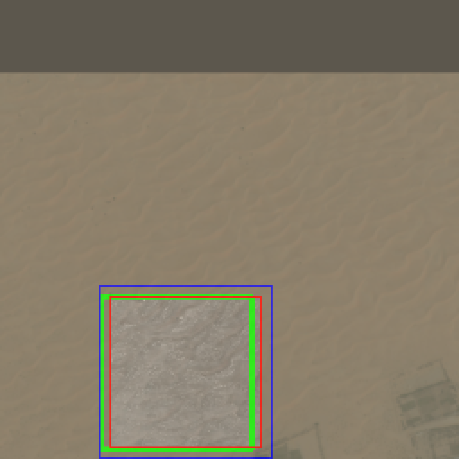
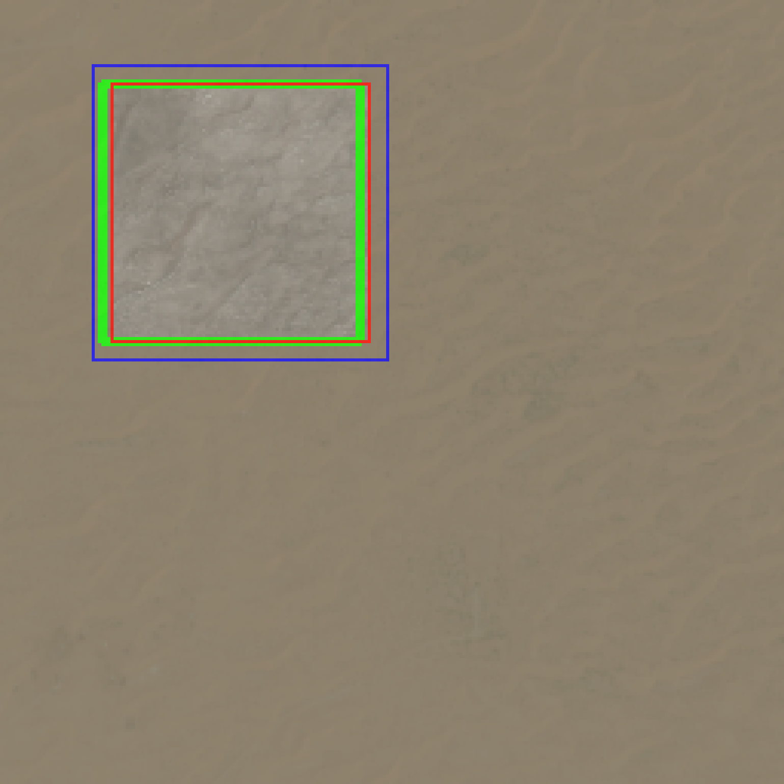
w/ bbox aug

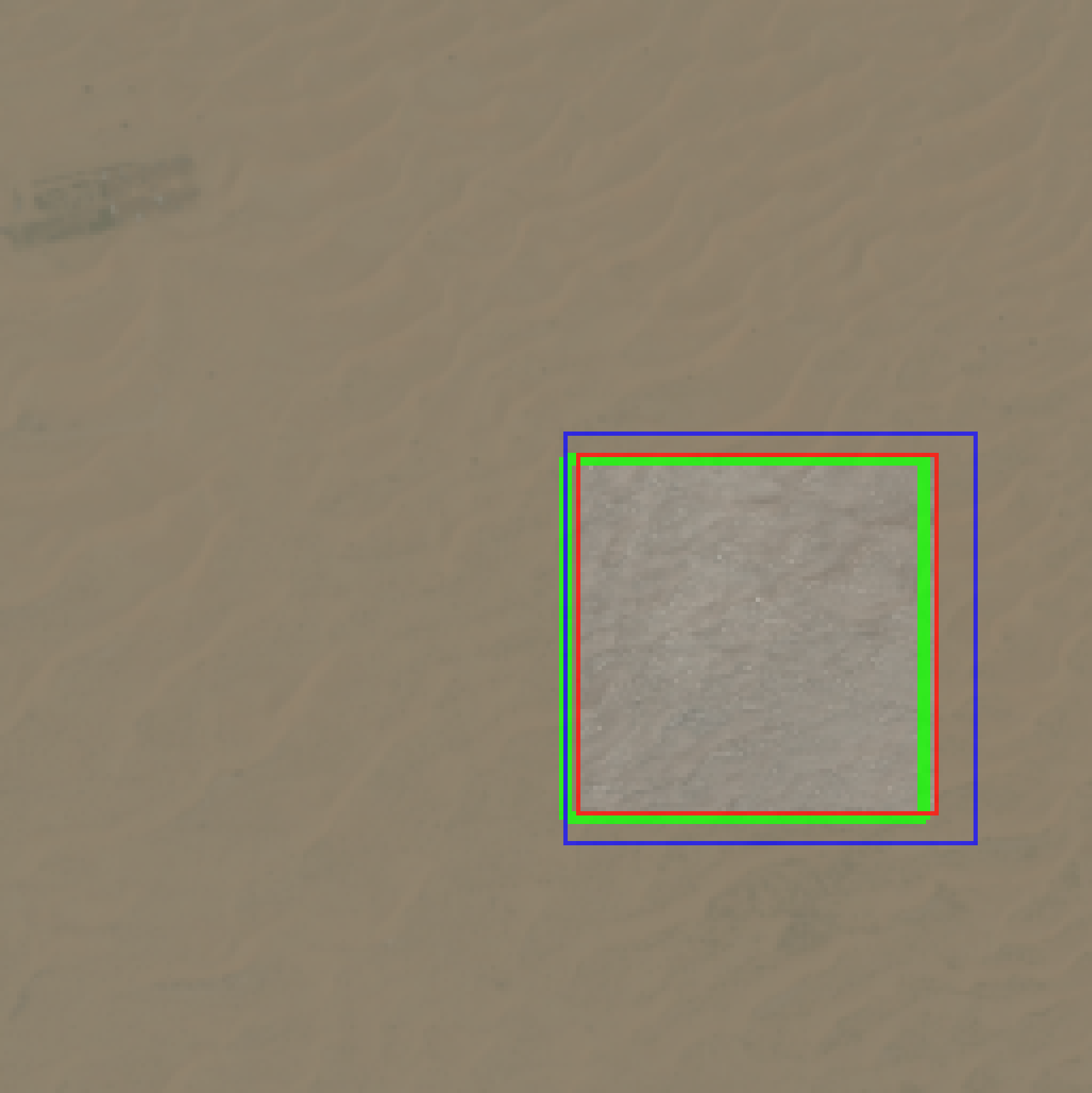
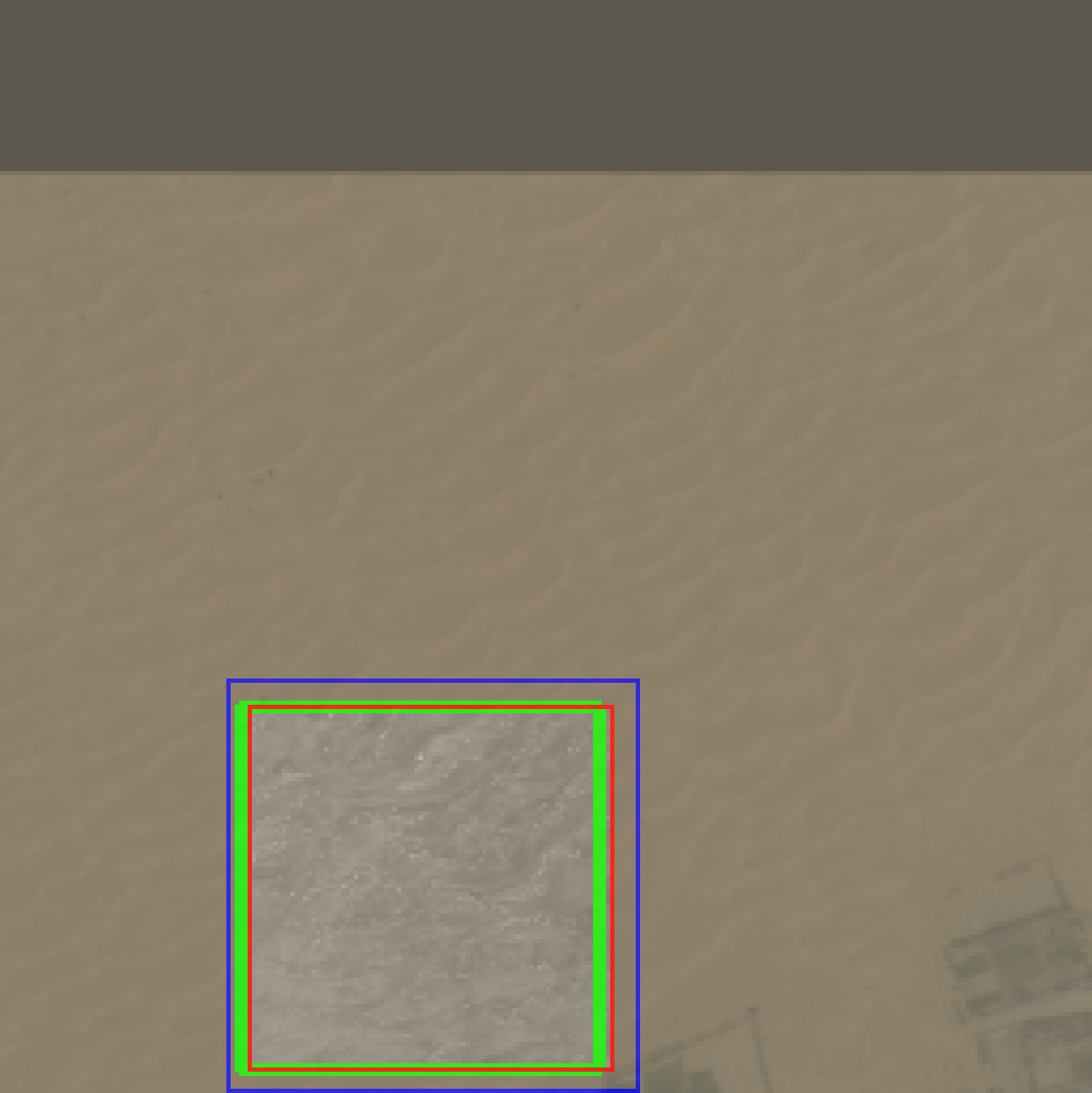
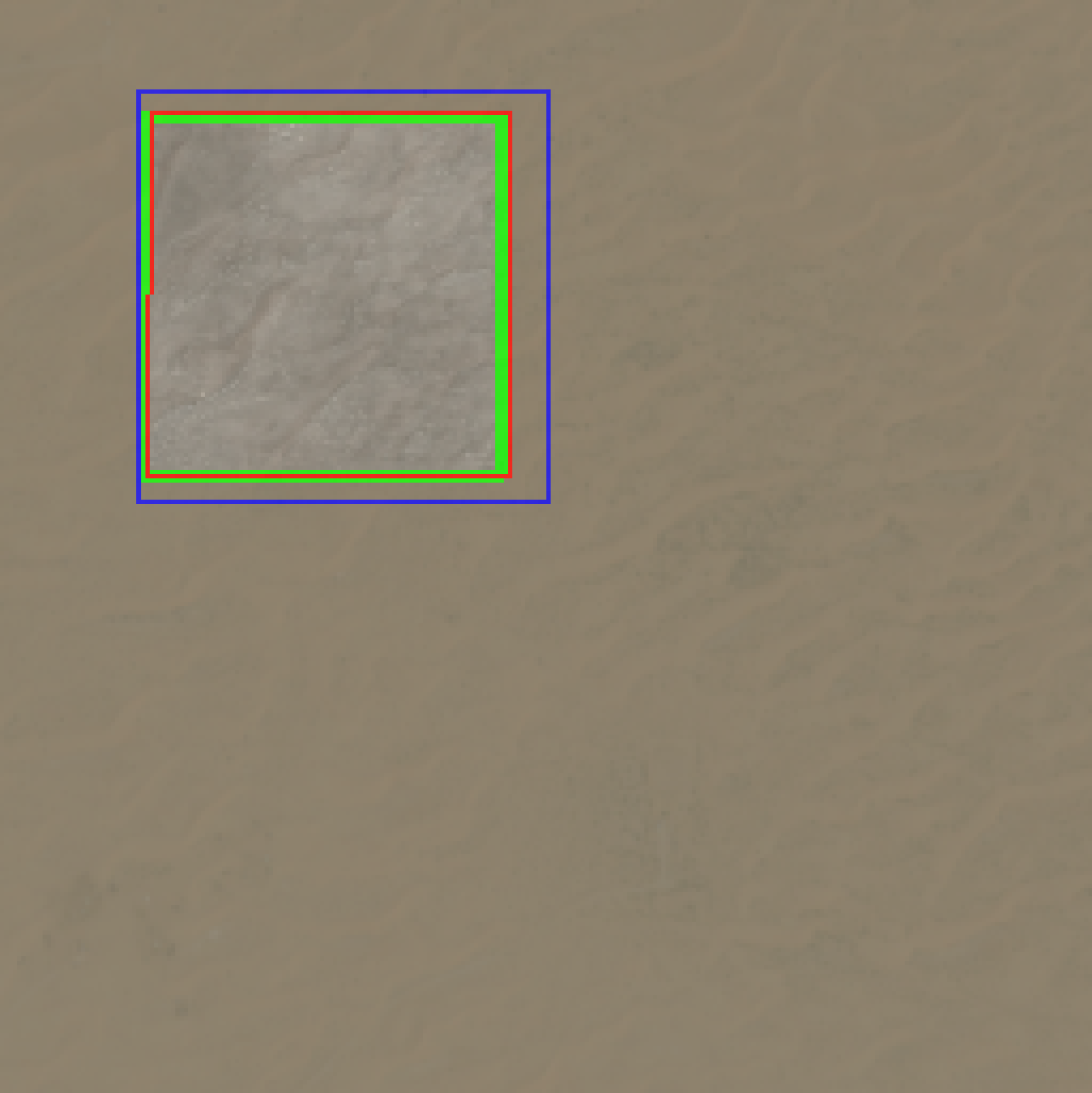
Figure 6: The qualitative comparison between finetuning the refinement module without bbox aug, with only bbox exp, and with bbox aug with $W_{S}=1536$. Green boxes are the ground truth, blue boxes are the bounding boxes from coarse alignment, and red boxes are final predictions after refinement.

TABLE III: Robustness evaluation with geometric noises, including rotation, resizing, and perspective transformation noises when $D_{C}=512$m and $W_{S}=1536$. ”Baseline” is our method with only translation.

	Ours (one stage)			Ours (two stages)
	Test MACE ($\mathrm{m}$)	Test CE ($\mathrm{m}$)		Test MACE ($\mathrm{m}$)	Test CE ($\mathrm{m}$)
Baseline	16.42	15.90		12.70	12.12
Rotation Noises
$5^{\circ}$	30.58	28.90		19.12	17.44
$10^{\circ}$	33.98	32.06		21.89	19.87
$30^{\circ}$	51.79	49.13		35.60	33.37
Resizing Noises
$0.1$	37.44	32.63		19.38	17.97
$0.2$	41.76	37.20		23.40	21.83
$0.3$	52.45	48.36		34.95	33.19
Perspective Transformation Noises
$8~{}$\mathrm{p}\mathrm{x}$$	34.97	31.51		19.47	17.60
$16~{}$\mathrm{p}\mathrm{x}$$	34.97	31.62		20.24	18.07
$32~{}$\mathrm{p}\mathrm{x}$$	39.01	35.48		23.46	20.54

One stage

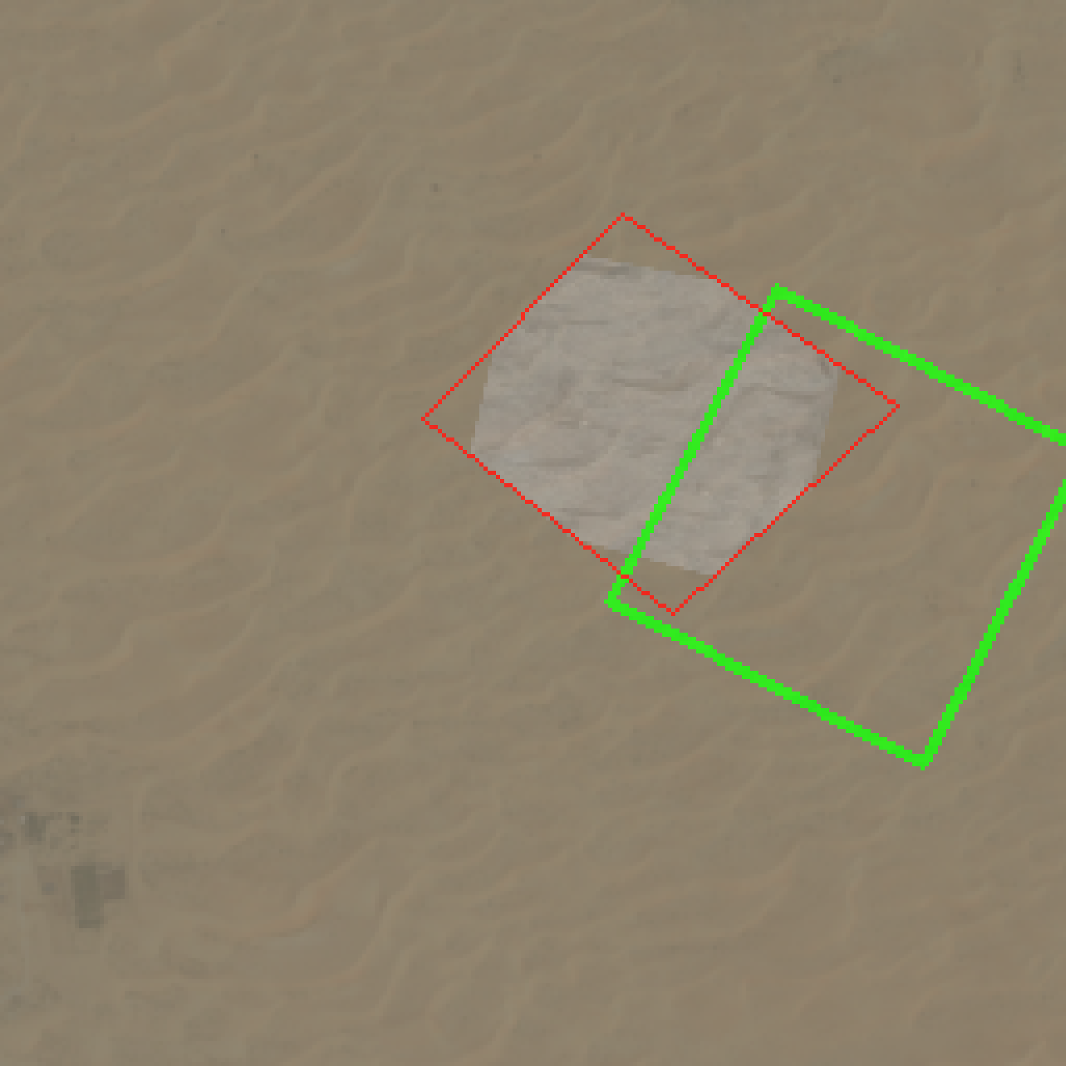
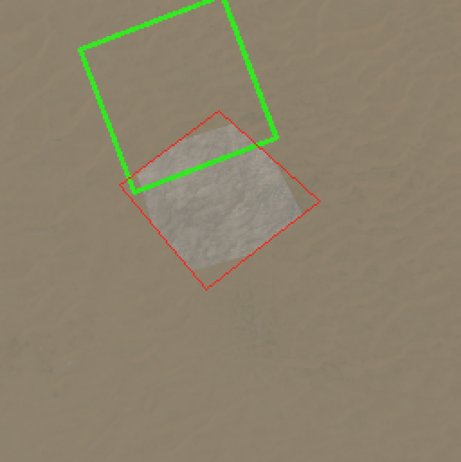
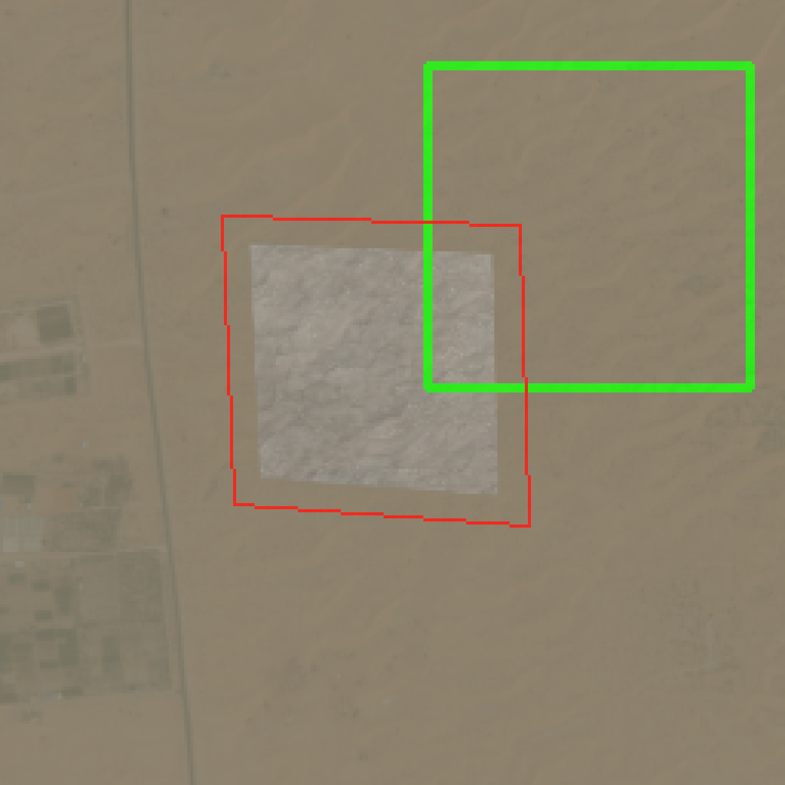
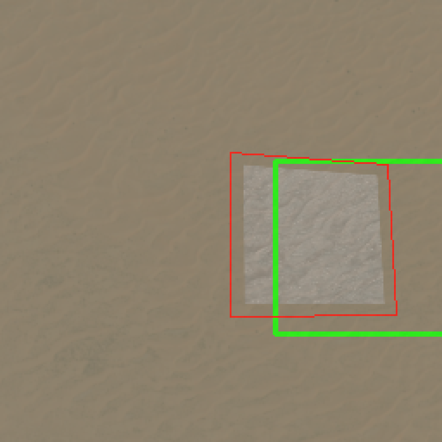
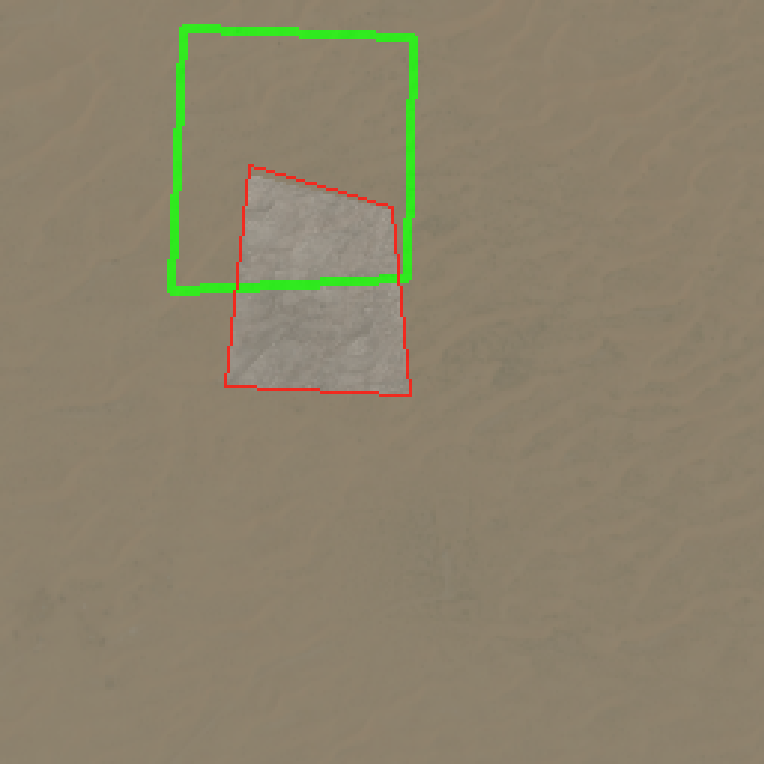
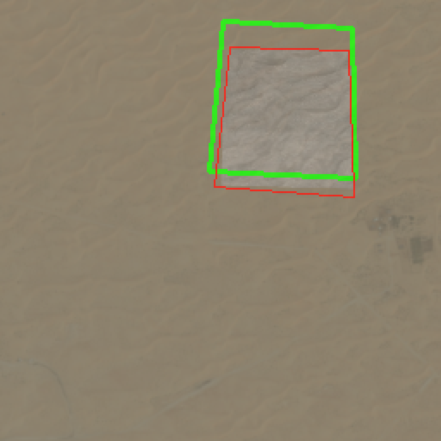
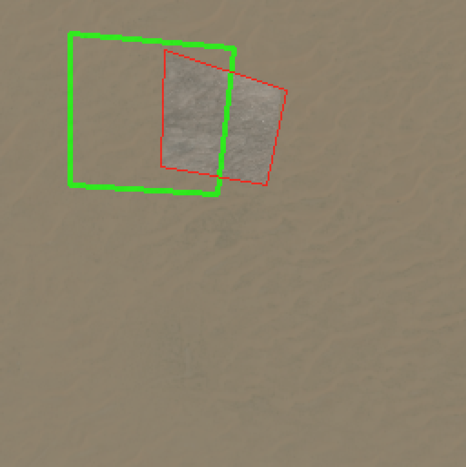
Two stages

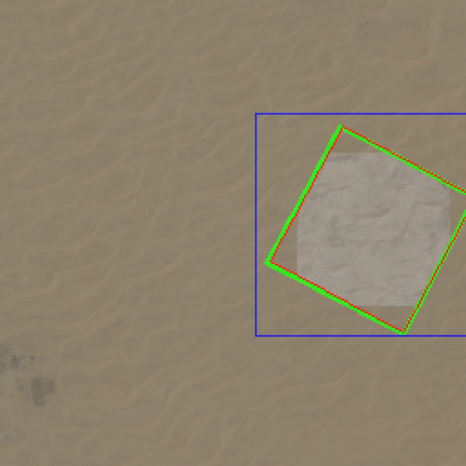
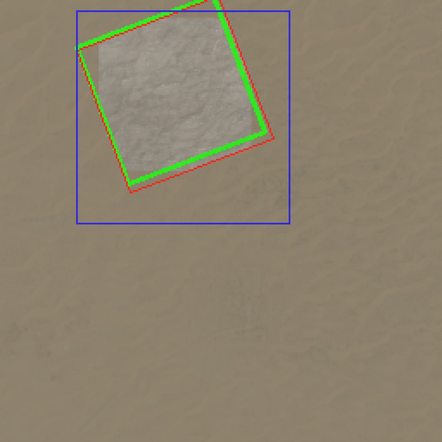
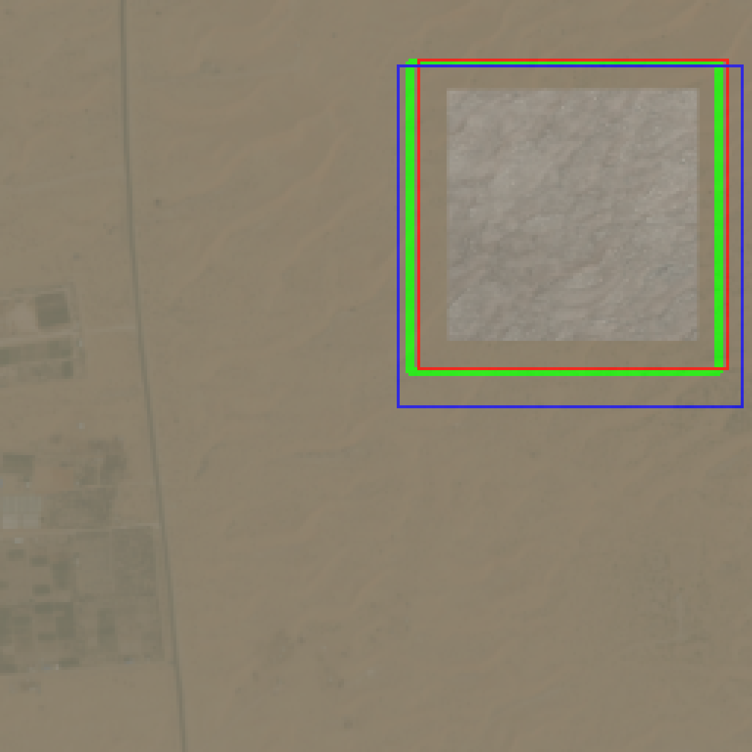
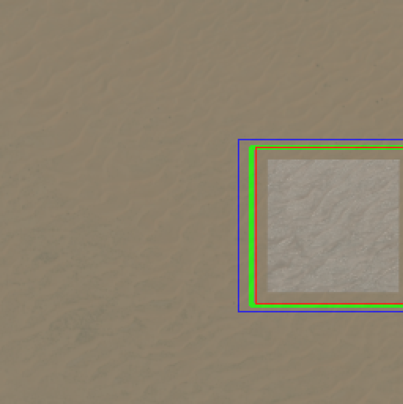
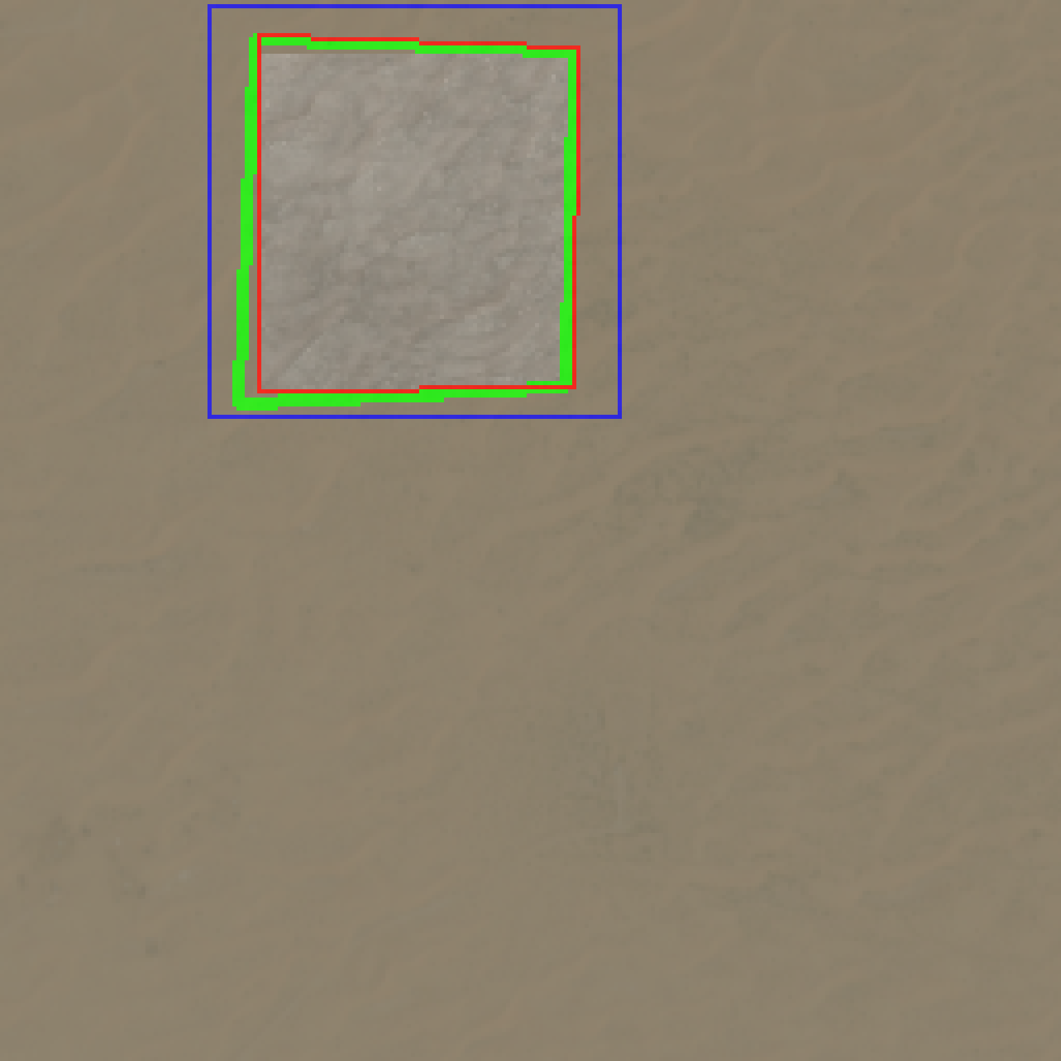
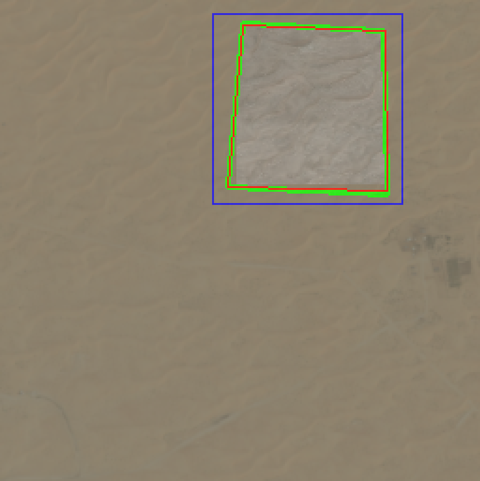
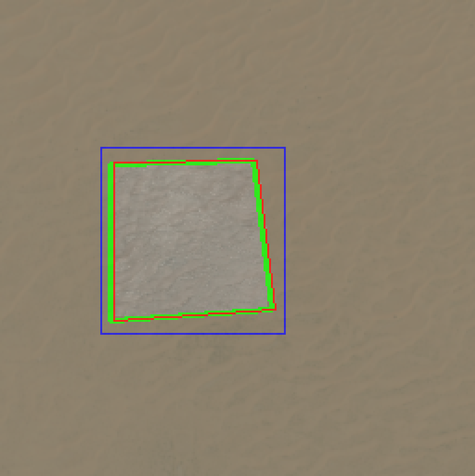
Figure 7: Visualization results with geometric noises for our one-stage and two-stage methods with $W_{S}=1536$ and $D_{C}=512$m. Green boxes are the ground truth, blue boxes are the bounding boxes from coarse alignment for our two-stage method, and red boxes are the final predictions of one-stage and two-stage methods. The $1^{\textrm{st}}$-$2^{\textrm{nd}}$ columns show rotation noises, the $3^{\textrm{rd}}$-$4^{\textrm{th}}$ columns show resizing noises, and the $5^{\textrm{th}}$-$8^{\textrm{th}}$ columns show perspective transformation noises.

VI Conclusions

In this paper, we presented a novel approach based on deep homography estimation for UAV thermal geo-localization tasks. We validate the capability of STHN to precisely align thermal images, captured by UAV onboard sensors, with large-scale satellite maps, achieving successful alignment even with a constant overlap of $11\%$. Additionally, we showcase STHN’s resilience to geometric distortions, which significantly enhances the reliability of geo-localization outcomes.

Our future endeavors will aim to develop a hierarchical geo-localization framework. This framework will integrate deep homography estimation for local matching with image-based matching techniques for broad-scale global matching, thereby building up universal geo-localization solutions.

References

- [1] D. C. Tsouros, S. Bibi, and P. G. Sarigiannidis, “A review on uav-based applications for precision agriculture,” Information, vol. 10, no. 11, p. 349, 2019.
- [2] M. Półka, S. Ptak, and Łukasz Kuziora, “The use of uav’s for search and rescue operations,” Procedia Engineering, vol. 192, pp. 748–752, 2017, 12th international scientific conference of young scientists on sustainable, modern and safe transport.
- [3] A. Saviolo, P. Rao, V. Radhakrishnan, J. Xiao, and G. Loianno, “Unifying foundation models with quadrotor control for visual tracking beyond object categories,” in IEEE International Conference on Robotics and Automation (ICRA), 2024.
- [4] J. Xing, G. Cioffi, J. Hidalgo-Carrió, and D. Scaramuzza, “Autonomous power line inspection with drones via perception-aware mpc,” in IEEE/RSJ International Conference on Intelligent Robots and Systems (IROS), 2023, pp. 1086–1093.
- [5] L. Morando, C. T. Recchiuto, J. Calla, P. Scuteri, and A. Sgorbissa, “Thermal and visual tracking of photovoltaic plants for autonomous uav inspection,” Drones, vol. 6, no. 11, 2022.
- [6] A. Couturier and M. A. Akhloufi, “A review on absolute visual localization for uav,” Robotics and Autonomous Systems, vol. 135, p. 103666, 2021.
- [7] Y. He, I. Cisneros, N. Keetha, J. Patrikar, Z. Ye, I. Higgins, Y. Hu, P. Kapoor, and S. Scherer, “Foundloc: Vision-based onboard aerial localization in the wild,” arXiv preprint arXiv:2310.16299, 2023.
- [8] A. T. Fragoso, C. T. Lee, A. S. McCoy, and S.-J. Chung, “A seasonally invariant deep transform for visual terrain-relative navigation,” Science Robotics, vol. 6, no. 55, p. eabf3320, 2021.
- [9] B. Patel, T. D. Barfoot, and A. P. Schoellig, “Visual localization with google earth images for robust global pose estimation of uavs,” in IEEE International Conference on Robotics and Automation (ICRA), 2020, pp. 6491–6497.
- [10] M. Shan, F. Wang, F. Lin, Z. Gao, Y. Z. Tang, and B. M. Chen, “Google map aided visual navigation for uavs in gps-denied environment,” in IEEE International Conference on Robotics and Biomimetics (ROBIO), 2015, pp. 114–119.
- [11] J. Xiao, D. Tortei, E. Roura, and G. Loianno, “Long-range uav thermal geo-localization with satellite imagery,” in IEEE/RSJ International Conference on Intelligent Robots and Systems (IROS), 2023, pp. 5820–5827.
- [12] S.-Y. Cao, J. Hu, Z. Sheng, and H.-L. Shen, “Iterative deep homography estimation,” in Proceedings of the IEEE/CVF Conference on Computer Vision and Pattern Recognition (CVPR), 2022, pp. 1879–1888.
- [13] D. DeTone, T. Malisiewicz, and A. Rabinovich, “Deep image homography estimation,” arXiv preprint arXiv:1606.03798, 2016.
- [14] J. Zhang, C. Wang, S. Liu, L. Jia, N. Ye, J. Wang, J. Zhou, and J. Sun, “Content-aware unsupervised deep homography estimation,” in Computer Vision – ECCV 2020, A. Vedaldi, H. Bischof, T. Brox, and J.-M. Frahm, Eds. Cham: Springer International Publishing, 2020, pp. 653–669.
- [15] Y. Zhao, X. Huang, and Z. Zhang, “Deep lucas-kanade homography for multimodal image alignment,” in Proceedings of the IEEE/CVF conference on computer vision and pattern recognition (CVPR), 2021, pp. 15 950–15 959.
- [16] R. Shao, G. Wu, Y. Zhou, Y. Fu, L. Fang, and Y. Liu, “Localtrans: A multiscale local transformer network for cross-resolution homography estimation,” in Proceedings of the IEEE/CVF international conference on computer vision (CVPR), 2021, pp. 14 890–14 899.
- [17] S.-Y. Cao, R. Zhang, L. Luo, B. Yu, Z. Sheng, J. Li, and H.-L. Shen, “Recurrent homography estimation using homography-guided image warping and focus transformer,” in Proceedings of the IEEE/CVF Conference on Computer Vision and Pattern Recognition (CVPR), June 2023, pp. 9833–9842.
- [18] H. Le, F. Liu, S. Zhang, and A. Agarwala, “Deep homography estimation for dynamic scenes,” in Proceedings of the IEEE/CVF conference on computer vision and pattern recognition (CVPR), 2020, pp. 7652–7661.
- [19] G. J. V. Dalen, D. P. Magree, and E. N. Johnson, “Absolute localization using image alignment and particle filtering,” in AIAA Guidance, Navigation, and Control Conference, 2016.
- [20] A. Yol, B. Delabarre, A. Dame, J.-E. Dartois, and E. Marchand, “Vision-based absolute localization for unmanned aerial vehicles,” in IEEE/RSJ International Conference on Intelligent Robots and Systems (IROS), 2014, pp. 3429–3434.
- [21] M. Mantelli, D. Pittol, R. Neuland, A. Ribacki, R. Maffei, V. Jorge, E. Prestes, and M. Kolberg, “A novel measurement model based on abbrief for global localization of a uav over satellite images,” Robotics and Autonomous Systems, vol. 112, pp. 304–319, 2019.
- [22] A. Shetty and G. X. Gao, “Uav pose estimation using cross-view geolocalization with satellite imagery,” in IEEE International Conference on Robotics and Automation (ICRA), 2019, pp. 1827–1833.
- [23] H. Goforth and S. Lucey, “Gps-denied uav localization using pre-existing satellite imagery,” in IEEE International Conference on Robotics and Automation (ICRA), 2019, pp. 2974–2980.
- [24] M. Bianchi and T. D. Barfoot, “Uav localization using autoencoded satellite images,” IEEE Robotics and Automation Letters, vol. 6, no. 2, pp. 1761–1768, 2021.
- [25] Y. LeCun, Y. Bengio, and G. Hinton, “Deep learning,” nature, vol. 521, no. 7553, pp. 436–444, 2015.
- [26] J. Delaune, R. Hewitt, L. Lytle, C. Sorice, R. Thakker, and L. Matthies, “Thermal-inertial odometry for autonomous flight throughout the night,” in IEEE/RSJ International Conference on Intelligent Robots and Systems (IROS), 2019, pp. 1122–1128.
- [27] V. Polizzi, R. Hewitt, J. Hidalgo-Carrió, J. Delaune, and D. Scaramuzza, “Data-efficient collaborative decentralized thermal-inertial odometry,” IEEE Robotics and Automation Letters, vol. 7, no. 4, pp. 10 681–10 688, 2022.
- [28] F. Achermann, A. Kolobov, D. Dey, T. Hinzmann, J. J. Chung, R. Siegwart, and N. Lawrance, “Multipoint: Cross-spectral registration of thermal and optical aerial imagery,” in Proceedings of the 2020 Conference on Robot Learning, ser. Proceedings of Machine Learning Research, J. Kober, F. Ramos, and C. Tomlin, Eds., vol. 155. PMLR, 16–18 Nov 2021, pp. 1746–1760.
- [29] N. Keetha, A. Mishra, J. Karhade, K. M. Jatavallabhula, S. Scherer, M. Krishna, and S. Garg, “Anyloc: Towards universal visual place recognition,” IEEE Robotics and Automation Letters, vol. 9, no. 2, pp. 1286–1293, 2023.
- [30] T. Nguyen, S. W. Chen, S. S. Shivakumar, C. J. Taylor, and V. Kumar, “Unsupervised deep homography: A fast and robust homography estimation model,” IEEE Robotics and Automation Letters, vol. 3, no. 3, pp. 2346–2353, 2018.
- [31] Y. Luo, X. Wang, Y. Wu, and C. Shu, “Infrared and visible image homography estimation using multiscale generative adversarial network,” Electronics, vol. 12, no. 4, 2023.
- [32] M. Mirza and S. Osindero, “Conditional generative adversarial nets,” arXiv preprint arXiv:1411.1784, 2014.
- [33] X. Wang, Y. Luo, Q. Fu, Y. He, C. Shu, Y. Wu, and Y. Liao, “Coarse-to-fine homography estimation for infrared and visible images,” Electronics, vol. 12, no. 21, 2023.
- [34] Z. Teed and J. Deng, “Raft: Recurrent all-pairs field transforms for optical flow,” in Computer Vision – ECCV 2020, A. Vedaldi, H. Bischof, T. Brox, and J.-M. Frahm, Eds. Cham: Springer International Publishing, 2020, pp. 402–419.
- [35] Y. Abdel-Aziz, H. Karara, and M. Hauck, “Direct linear transformation from comparator coordinates into object space coordinates in close-range photogrammetry,” Photogrammetric Engineering & Remote Sensing, vol. 81, no. 2, pp. 103–107, 2015.
- [36] I. Loshchilov and F. Hutter, “Decoupled weight decay regularization,” in International Conference on Learning Representations, 2019.
- [37] D. G. Lowe, “Distinctive image features from scale-invariant keypoints,” International journal of computer vision, vol. 60, no. 2, pp. 91–110, 2004.
- [38] M. A. Fischler and R. C. Bolles, “Random sample consensus: a paradigm for model fitting with applications to image analysis and automated cartography,” Commun. ACM, vol. 24, no. 6, p. 381–395, jun 1981.
- [39] D. Baráth, J. Noskova, M. Ivashechkin, and J. Matas, “Magsac++, a fast, reliable and accurate robust estimator,” in IEEE/CVF Conference on Computer Vision and Pattern Recognition (CVPR), 2020, pp. 1301–1309.
- [40] E. Rublee, V. Rabaud, K. Konolige, and G. Bradski, “Orb: An efficient alternative to sift or surf,” in International Conference on Computer Vision (ICCV), 2011, pp. 2564–2571.
- [41] S. Leutenegger, M. Chli, and R. Y. Siegwart, “Brisk: Binary robust invariant scalable keypoints,” in International Conference on Computer Vision (ICCV), 2011, pp. 2548–2555.
- [42] R. Arandjelović, P. Gronat, A. Torii, T. Pajdla, and J. Sivic, “Netvlad: Cnn architecture for weakly supervised place recognition,” IEEE Transactions on Pattern Analysis and Machine Intelligence, vol. 40, no. 6, pp. 1437–1451, 2018.
- [43] F. Radenović, G. Tolias, and O. Chum, “Fine-tuning cnn image retrieval with no human annotation,” IEEE Transactions on Pattern Analysis and Machine Intelligence, vol. 41, no. 7, pp. 1655–1668, 2019.
- [44] M. Oquab, T. Darcet, T. Moutakanni, H. Vo, M. Szafraniec, V. Khalidov, P. Fernandez, D. Haziza, F. Massa, A. El-Nouby et al., “Dinov2: Learning robust visual features without supervision,” arXiv preprint arXiv:2304.07193, 2023.
- [45] H. Jégou, M. Douze, C. Schmid, and P. Pérez, “Aggregating local descriptors into a compact image representation,” in IEEE/CVF Conference on Computer Vision and Pattern Recognition (CVPR), 2010, pp. 3304–3311.