On Calibration of Object Detectors: Pitfalls, Evaluation and Baselines

Abstract

Reliable usage of object detectors require them to be calibrated—a crucial problem that requires careful attention. Recent approaches towards this involve (1) designing new loss functions to obtain calibrated detectors by training them from scratch, and (2) post-hoc Temperature Scaling (TS) that learns to scale the likelihood of a trained detector to output calibrated predictions. These approaches are then evaluated based on a combination of Detection Expected Calibration Error (D-ECE) and Average Precision. In this work, via extensive analysis and insights, we highlight that these recent evaluation frameworks, evaluation metrics, and the use of TS have notable drawbacks leading to incorrect conclusions. As a step towards fixing these issues, we propose a principled evaluation framework to jointly measure calibration and accuracy of object detectors. We also tailor efficient and easy-to-use post-hoc calibration approaches such as Platt Scaling and Isotonic Regression specifically for object detection task. Contrary to the common notion, our experiments show that once designed and evaluated properly, post-hoc calibrators, which are extremely cheap to build and use, are much more powerful and effective than the recent train-time calibration methods. To illustrate, D-DETR with our post-hoc Isotonic Regression calibrator outperforms the recent train-time state-of-the-art calibration method Cal-DETR [munir2023caldetr] by more than $7$ D-ECE on the COCO dataset. Additionally, we propose improved versions of the recently proposed Localization-aware ECE [saod] and show the efficacy of our method on these metrics as well. Code is available at: https://github.com/fiveai/detection_calibration.

1 Introduction

Object detectors have been widely-used in a variety of safety-critical applications related to, but not limited to, autonomous driving [geiger2012kitti, caesar2020nuscenes, sun2020scalability, grigorescu2019surveyAD, Cityscapes, bdd100k] and medical imaging [yan2017deeplesion, kumar2020multiorgan, kumar2017pathology, jin2022anatomy]. In addition to being accurate, their confidence estimates should also allow characterization of their error behaviour to make them reliable. This feature, known as calibration, can enable a model to provide valuable information to subsequent systems playing crucial role in making safety-critical decisions [karimi2020medical, mehrtash2020medical_calibration, lu2017associationlstm, sam, bewley2016SORT]. Despite its importance, calibration of detectors is a relatively underexplored area in the literature and requires significant attention. Therefore, in this work, we focus on different aspects of the evaluation framework that is now being adopted by most recent works building calibrated detectors and discuss their pitfalls and propose fixes. Additionally, we tailor the well-known post-hoc calibration methods to improve the calibration of a given object detector (trained) with minimal effort.

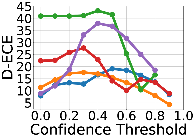
(a) D-ECE

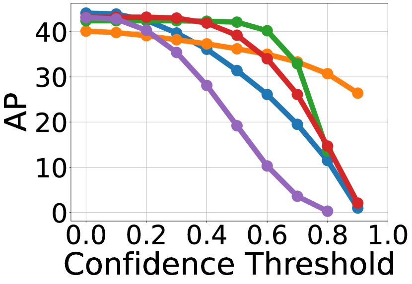
(b) AP

(c) $\mathrm{LaECE_{0}}$

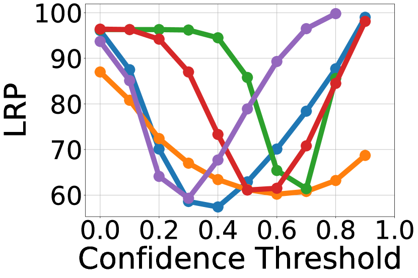
(d) LRP

Figure 1: The performance of different detectors over operating confidence thresholds on COCO minitest. Orange: Faster R-CNN, Green: RS R-CNN, Purple: ATSS, Red: PAA, Blue: D-DETR. All measures are lower better except AP. It is not trivial to identify an operating threshold and compare detectors, especially when the common evaluation [CalibrationOD, munir2022tcd, MCCL, munir2023bpc, munir2023caldetr], combining D-ECE for calibration and AP for accuracy, is used. Instead, we use $\mathrm{LaECE_{0}}$ and LRP.

Naturally, practitioners prefer detectors that perform well in terms of both accuracy and calibration, which we refer to as joint performance. However, unlike classification, choosing the best performing model is non-trivial for object detection. This is because different detectors commonly yield detection sets with varying cardinalities for the same image, and this difference in population size is shown to affect the joint performance evaluation [saod]. Furthermore, when object detectors are used in practice, an operating threshold is normally chosen [karimi2020medical, mehrtash2020medical_calibration, lu2017associationlstm, sam, groundingdino, glip, bewley2016SORT], and the choice of this threshold directly influences a detector’s performance. Thus, comparing the performance of a detector in terms of calibration or accuracy over different operating thresholds, as well as with different detectors, is not straightforward as illustrated in fig. 1.

We assert that a framework for joint evaluation should follow certain basic principles. Firstly, the detectors should be evaluated on a thresholded set of detections to align with their practical usage. While doing so, the evaluation framework will require a principled model-dependent threshold selection mechanism, as the confidence distribution of each detector can differ significantly [LRPPAMI]. Secondly, the calibration evaluation should involve fine-grained information about the detection quality. For example, if the confidence score represents the localisation quality of a detection, this provides more fine-grained information than only representing whether the object is detected or not. Thirdly, the datasets should be properly-designed for evaluation. That is, the training, validation (val.) and in-distribution (ID) test splits should be sampled from the same underlying distribution, and additionally, the domain-shifted test splits — which are crucial for safety-critical applications — should be included. Finally, baseline detectors and calibration methods must be trained properly, as otherwise the evaluation might provide misleading conclusions.

There are three approaches in the literature attempting joint evaluation of accuracy and calibration as follows:

• D-ECE-style [CalibrationOD, munir2022tcd, MCCL, munir2023bpc, munir2023caldetr]: thresholds the detections commonly from a confidence of $0.30$ to compute Detection Expected Calibration Error (D-ECE) and use top-100 detections from each image for Average Precision (AP),

• LaECE-style [saod]: enforces the detectors to be thresholded properly, and combine Localisation-aware Expected Calibration Error (LaECE) with LRP [LRPPAMI],

• CE-style [popordanoska2024CE]: thresholds the detections from a confidence score of $0.50$ to obtain Calibration Error (CE) and AP.

As summarized in table 1, these evaluations do not adhere to the basic principles mentioned above. To exemplify, D-ECE-style evaluation — the most common evaluation approach [CalibrationOD, munir2022tcd, MCCL, munir2023bpc, munir2023caldetr] — uses different operating thresholds for calibration and accuracy, which does not align well with the practical usage of detectors. Also, using a fixed threshold for all detectors artificially promotes certain detectors. To illustrate, while D-ECE-style evaluation (threshold 0.3) ranks the green detector as the worst in fig. 1(a), the green one yields the best D-ECE at $0.70$. Besides, as shown in fig. 1(b), AP is maximized at the confidence of $0$ (leading to too many detections with low confidences) for all the detectors, and thus AP cannot be used to obtain a proper operating threshold [LRPPAMI, saod]. In terms of conveying fine-grained information, D-ECE aims to align confidence with the precision only, which effectively ignores the localisation quality of the detections, a crucial performance aspect of object detection. Finally, this type of evaluation also has limitations in terms of dataset splits and the chosen baselines as we explore in section 3.

Having proper baseline calibration methods is also essential to monitor the progress in the field. Recently proposed train-time calibration methods commonly employ an auxiliary loss term to regularize the confidence scores during training [CalibrationOD, munir2022tcd, MCCL, munir2023bpc, munir2023caldetr]. Such methods are shown to be effective against the Temperature Scaling (TS) [calibration], which is used as the only post-hoc calibration baseline. Post-hoc calibrators are obtained on a held-out val. set, and hence can easily be applied to any off-the-shelf detector. Despite their potential advantages, unlike for classification [calibration, rahimi2022posthoc, ma2021metacal, hekler2023calibration, wang2021rethinkcalibration, zhang2023transferablecalibration, joy2023adaptive], post-hoc calibration methods have not been explored for object detection sufficiently [CalibrationOD, saod].

Table 1: Principles of joint performance evaluation of object detectors in terms of accuracy and calibration, and whether existing evaluation approaches violate them.

Principles of Joint Evaluation	D-ECE-style [CalibrationOD, MCCL, munir2023bpc, munir2022tcd, munir2023caldetr]	LaECE-style [saod]	CE-style [popordanoska2024CE]	Ours
Model-dependent threshold selection	✗	✓	✗	✓
Fine-grained confidence scores	✗	✗	✗	✓
Properly-designed datasets	✗	✗	✗	✓
Properly-trained detectors & calibrators	✗	✓	✗	✓

In this paper, we introduce a joint evaluation framework which respects the aforementioned principles (table 1), and thus address the critical drawbacks of existing evaluation approaches. That is, we first define $\mathrm{LaECE}_{0}$ and $\mathrm{LaACE}_{0}$, as novel calibration errors, each of which aims to align the detection confidence scores with their localisation qualities. Specifically, the detectors respecting $\mathrm{LaECE}_{0}$ and $\mathrm{LaACE}_{0}$ provide quite informative confidence estimates about their behaviours. We measure accuracy using LRP [LRPPAMI], which requires a proper combination of false-positive (FP), false-negative (FN) and localisation errors. Thereby requiring the detectors to be properly-thresholded as shown by the bell-like curves in fig. 1(d). Also, we design three datasets with different characteristics, and introduce Platt Scaling (PS) as well as Isotonic Regression (IR) as highly effective post-hoc calibrators tailored to object detection. Our main contributions are:

• We identify various quirks and assumptions in state-of-the-art (SOTA) methods in quantifying miscalibration of object detectors and show that they, if not treated properly, can provide misleading conclusions.

• We introduce a framework for joint evaluation consisting of properly-designed datasets, evaluation measures tailored to practical usage of object detectors and baseline post-hoc calibration methods. We show that our framework addresses the drawbacks of existing approaches.

• In contrast to the literature, we show that, if designed properly, post-hoc calibrators can significantly outperform the SOTA training time calibration methods. To illustrate, on the common COCO benchmark, D-DETR with our IR calibrator outperforms the SOTA Cal-DETR [munir2023caldetr] significantly: (i) by more than $7$ points in terms of D-ECE and (ii) $\sim 4$ points in terms of our challenging $\mathrm{LaECE}_{0}$

2 Background and Notation

Object Detectors and Evaluating their Accuracy Denoting the set of $M$ objects in an image $X$ by $\{b_{i},c_{i}\}^{M}$ where $b_{i}\in\mathbb{R}^{4}$ is a bounding box and $c_{i}\in\{1,\dots,K\}$ is its class; an object detector produces the bounding box $\hat{b}_{i}$, the class label $\hat{c}_{i}$ and the confidence score $\hat{p}_{i}$ for the objects in $X$, i.e., $f(X)=\{\hat{c}_{i},\hat{b}_{i},\hat{p}_{i}\}^{N}$ with $N$ being the number of predictions. During evaluation, each detection is first labelled as a true-positive (TP) or a FP using a matching function $\psi(\cdot)$ relying on an Intersection-over-Union (IoU) threshold $\tau$ to validate TPs. We assume $\psi(i)$ returns the index of the object that a TP $i$ matches to; else $i$ is a FP and $\psi(i)=-1$. Then, AP [COCO, LVIS, PASCAL], the common accuracy measure, corresponds to the area under the Precision Recall (PR) curve. Though widely-used, AP has been criticized recently from different aspects [LRPPAMI, TIDE, Trustworthy, LRP, OptCorrCost]. To illustrate, AP is maximized when the number of detections increases [saod] as shown in fig. 1(b). Therefore, AP does not help choosing an operating threshold, which is critical for practical deployment. As an alternative, LRP [LRP, LRPPAMI] combines the numbers of TP, FP, FN with the localisation error of the detections, which are denoted by $\mathrm{N_{TP}}$, $\mathrm{N_{FP}}$, $\mathrm{N_{FN}}$ and $\mathcal{E}_{loc}(i)\in[0,1]$ respectively:

$$\mathrm{LRP}=\frac{1}{\mathrm{N_{FP}}+\mathrm{N_{FN}}+\mathrm{N_{TP}}}\left(\mathrm{N_{FP}}+\mathrm{N_{FN}}+\sum\limits_{\psi(i)>0}\mathcal{E}_{loc}(i)\right).$$ (1)

Unlike AP, LRP requires the detection set to be thresholded properly as both FPs and FNs are penalized in Eq. (1).

Evaluating the Calibration of Object Detectors The alignment of accuracy and confidence of a model, termed calibration, is extensively studied for classification  [calibration, AdaptiveECE, verifiedunccalibration, rethinkcalibration, FocalLoss_Calibration, calibratepairwise]. That is, a classifier is calibrated if its accuracy is $p$ for the predictions with confidence of $p$ for all $p\in[0,1]$. For object detection, [CalibrationOD] extends this definition to enforce that the confidence matches the precision of the detector, $\mathbb{P}(\hat{c}_{i}=c_{i}|\hat{p}_{i})=\hat{p}_{i},\forall\hat{p}_{i}\in[0,1],$ where $\mathbb{P}(\hat{c}_{i}=c_{i}|\hat{p}_{i})$ is the precision. Then, discretizing the confidence space into $J$ bins, D-ECE is

$$\text{\lx@glossaries@gls@link{acronym}{DECE}{\leavevmode D-ECE}}=\sum_{j=1}^{J}\frac{|\hat{\mathcal{D}}_{j}|}{|\hat{\mathcal{D}}|}\left\lvert\bar{p}_{j}-\mathrm{precision}(j)\right\rvert,$$ (2)

where $\hat{\mathcal{D}}$ and $\hat{\mathcal{D}}_{j}$ are the set of all detections and the detections in the $j$-th bin, and $\bar{p}_{j}$ and $\mathrm{precision}(j)$ are the average confidence and the precision of the detections in the $j$-th bin. Alternatively, considering that object detection is a joint task of classification and localisation, LaECE [saod] aims to match the confidence with the product of precision and average IoU of TPs. Also, to prevent certain classes from dominating the error, LaECE is introduced as a class-wise measure. Using superscript $c$ to refer to each class and $\bar{\mathrm{IoU}}^{c}(j)$ as the average IoU of $\hat{\mathcal{D}}^{c}_{j}$, LaECE is defined as:

$$\mathrm{LaECE}=\frac{1}{K}\sum_{c=1}^{K}\sum_{j=1}^{J}\frac{|\hat{\mathcal{D}}^{c}_{j}|}{|\hat{\mathcal{D}}^{c}|}\left\lvert\bar{p}^{c}_{j}-\mathrm{precision}^{c}(j)\times\bar{\mathrm{IoU}}^{c}(j)\right\rvert.$$ (3)

Calibration Methods in Object Detection The existing methods for calibrating object detectors can be split into two groups:

(1) Training-time calibration approaches [munir2022tcd, MCCL, munir2023bpc, munir2023caldetr, popordanoska2024CE] regularize the model to yield calibrated confidence scores during training, which is generally achieved by an additive auxiliary loss.

(2) Post-hoc calibration methods use a held-out val. set to fit a calibration function that maps the predicted confidence to the calibrated confidence. Specifically, TS [calibration] is the only method considered as a baseline for recent training time methods [munir2022tcd, MCCL, munir2023bpc, popordanoska2024CE]. As an alternative, IR [zadrozny2002transforming] is used within a limited scope for a specific task called Self-aware Object Detection [saod]. Furthermore, its effectiveness neither on a wide range of detectors nor against existing training-time calibration approaches has yet been investigated.

3 Analysis of the Common D-ECE-style Evaluation

Figure 2: Comparison of calibration methods in terms of D-ECE on COCO mini-test using D-DETR [DDETR]. Post-hoc calibrators TS and IR are obtained on a subset of Objects365 [Objects365] following D-ECE-style evaluation.

D-ECE-style evaluation is the most common evaluation approach adopted by several methods [CalibrationOD, munir2022tcd, MCCL, munir2023bpc, munir2023caldetr]. For that reason, here we provide a comprehensive analysis of this evaluation approach and analyse the LaECE-style and CE-style evaluations in App. LABEL:app:analyses. Our analyses, based on the principles outlined in section 1 and table 1, show that all approaches have notable drawbacks.

1. Model-dependent threshold selection. As AP is obtained using the top-100 detections and D-ECE is computed on detections thresholded above $0.30$, D-ECE-style evaluation uses two different detection sets. This inconsistency is not reflective of how detectors are used in practice. Also, we observe that a fixed threshold of $0.30$ for evaluating the calibration induces a bias for certain detectors. To illustrate, we compare the performance of different calibration methods over different thresholds in fig. 2, where Cal-DETR [munir2023caldetr] performs the best only for the threshold $0.30$ and the post-hoc TS significantly outperforms it on all other thresholds. Therefore, this method of evaluation is sensitive to the choice of threshold, leading to ambiguity on the best performing method.

2. Fine-grained confidence scores. Manipulating Eq. (2), we show in App. LABEL:app:analyses that D-ECE for the $j$-th bin can be expressed as,

$$\Bigg{\lvert}\sum_{\begin{subarray}{c}\hat{b}_{i}\in\hat{\mathcal{D}}_{j},\psi(i)>0\end{subarray}}\big{(}\hat{p}_{i}-1\big{)}+\sum_{\begin{subarray}{c}\hat{b}_{i}\in\hat{\mathcal{D}}_{j},\psi(i)=-1\end{subarray}}\hat{p}_{i}\Bigg{\rvert}.$$ (4)

Eq. (4) implies that D-ECE is minimized when the confidence scores $\hat{p}_{i}$ of TPs are $1$ and those of FPs are $0$, which is also how the prediction-target pairs are usually constructed to train post-hoc TS [CalibrationOD, munir2022tcd, MCCL, munir2023bpc, munir2023caldetr]. Even if the detector is perfectly calibrated for these binary targets, the confidence scores do not provide information about localisation quality as illustrated by binary-valued $\hat{p}_{\mathrm{\text{\lx@glossaries@gls@link{acronym}{DECE}{\leavevmode D-ECE}}}}$ for both detections in fig. 3(b). Also, Popordanoska et al. [popordanoska2024CE] utilise D-ECE in a COCO-style manner, that is they average D-ECE over different TP validation IoU thresholds similar to COCO-style AP [COCO]. However, we observe that this way of using D-ECE can promote ambiguous confidence scores. As an example, given two IoU thresholds $\tau_{1}$ and $\tau_{2}$, a detection $\hat{b}_{i}$ with $\tau_{1}\leq\mathrm{IoU}(\hat{b}_{i},b_{\psi(i)})<\tau_{2}$ is a TP for $\tau_{1}$ but a FP for $\tau_{2}$. Thus, given Eq. (4), it follows that $\hat{b}_{i}$ has contradictory confidence targets for $\tau_{1}$ and $\tau_{2}$. This is illustrated in fig. 3(d) in which $\mathrm{\text{\lx@glossaries@gls@link{acronym}{DECE}{\leavevmode D-ECE}}_{C}}$ (red line) remains constant regardless of the confidence. Thus, using D-ECE (or another calibration measure) in this way should be avoided.

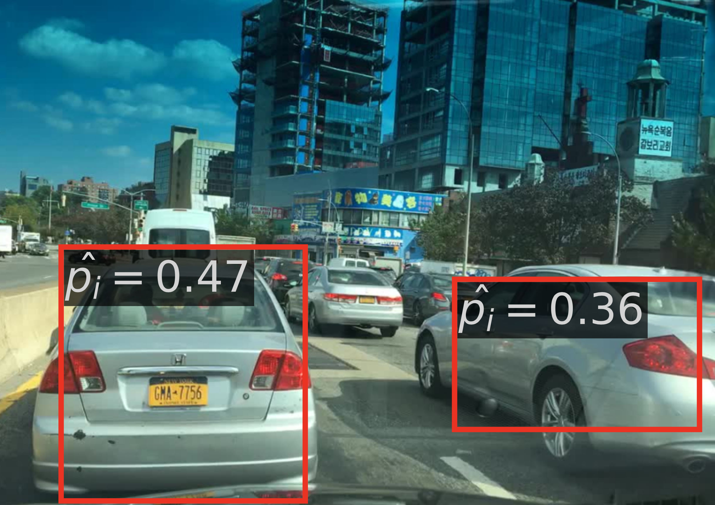
(a) Uncalibrated detections

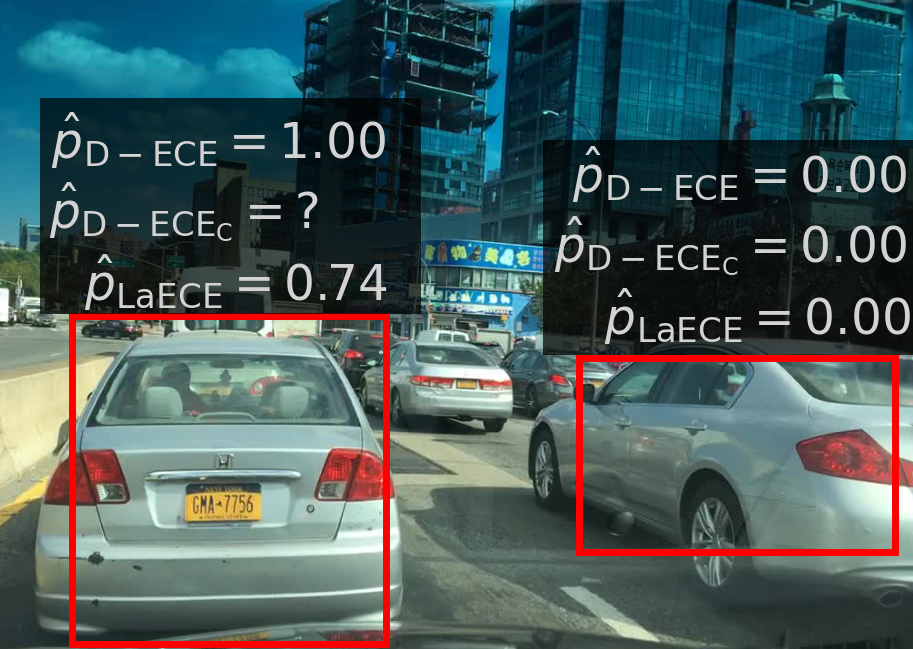
(b) Calibrated detections

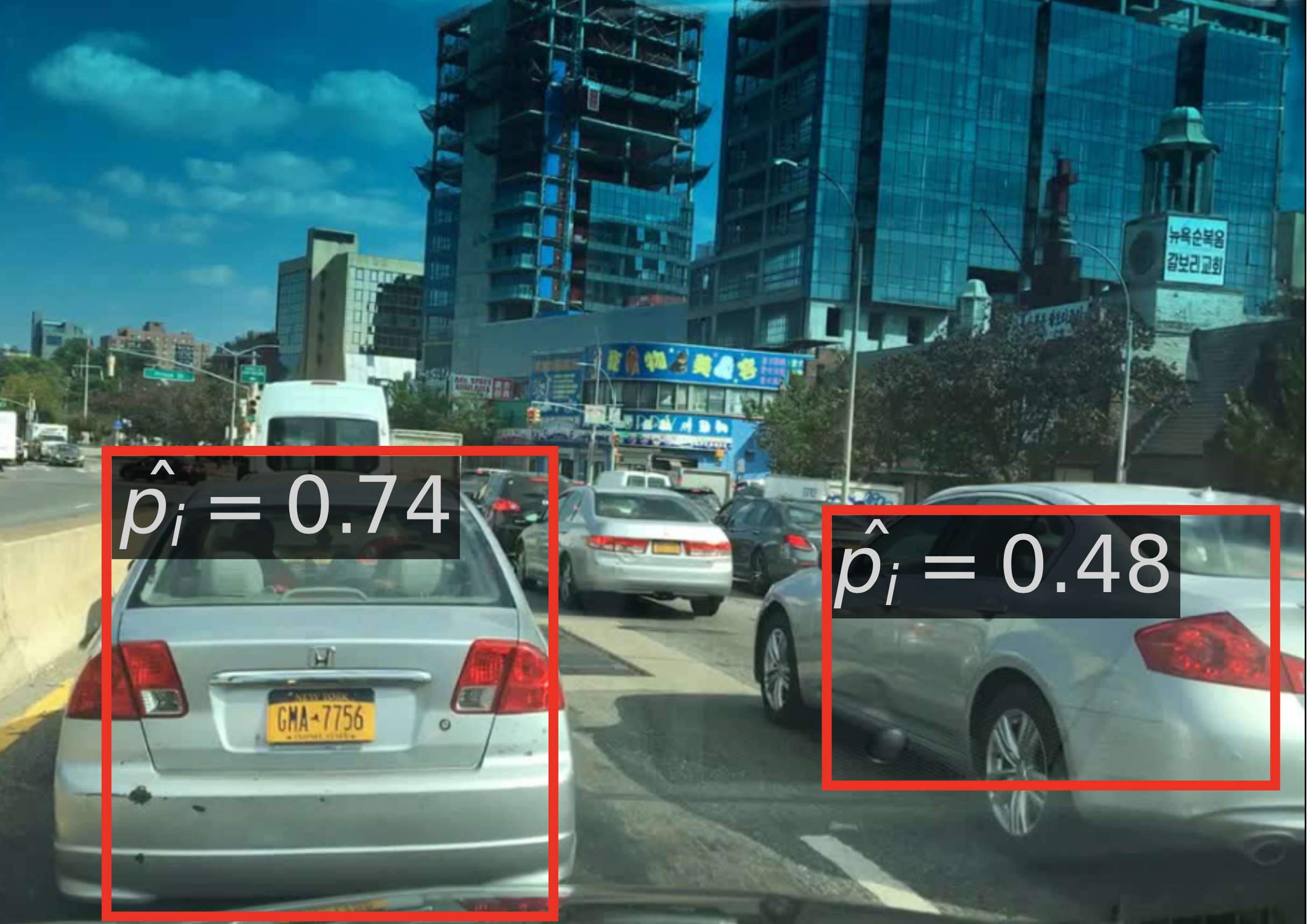
(c) Calibrated detections (Ours)

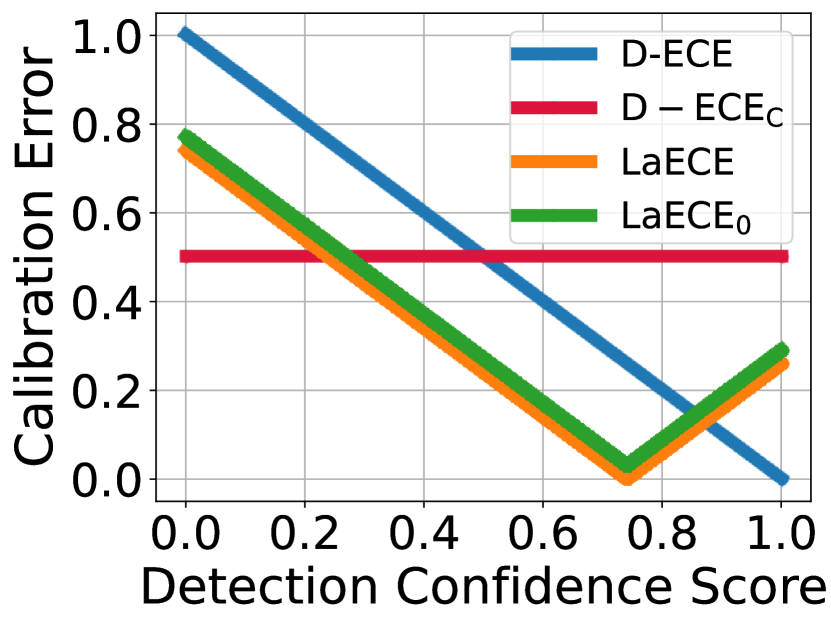
(d) TP for $\tau=0.5$

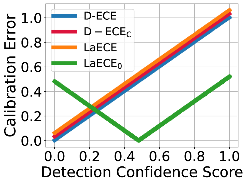
(e) FP for $\tau=0.5$, TP for $\tau=0$

(f) FP for $\tau=0$

Figure 3: A pictorial comparison of the different calibration errors. (a) Uncalibrated detections of D-DETR on an image from [bdd100k]. The detections on the left and right have IoUs of $0.74$ and $0.48$ with the objects. (b) Calibrated detections in terms of D-ECE and $\mathrm{LaECE}$ using $\tau=0.50$, and $\mathrm{\text{\lx@glossaries@gls@link{acronym}{DECE}{\leavevmode D-ECE}}_{C}}$, COCO-style D-ECE as in [popordanoska2024CE]. $\mathrm{D-ECE_{C}}=?$ as calibration error does not have a global minimum as shown in (d). (c) Calibrated detections in terms of $\mathrm{LaECE_{0}}$ and $\mathrm{LaACE_{0}}$ in which confidence matches IoU. (d-f) Calibration errors for different types of detections, for which $\mathrm{LaACE_{0}}$ behave the same as $\mathrm{LaECE_{0}}$, hence excluded for clarity. App. LABEL:app:analyses presents the details.

Table 2: Effect of using domain-shifted val. set on IR calibrator. Results are reported on COCO-minitest. Val. set is N/A for uncalibrated D-DETR and training time calibration method Cal-DETR.

Method	Val set	D-ECE	AP $\uparrow$
D-DETR	N/A	$12.8$	$44.1$
Cal-DETR	N/A	$8.7$	$44.4$
IR	Objects365	$14.2$	$44.1$
IR	COCO	$\mathbf{1.3}$ (+7.4)	$44.1$

Table 3: COCO training settings are commonly adopted while training D-DETR on Cityscapes. When trained with larger images and longer, DETR performs slightly better than Cal-DETR.

Method	Training Style	D-ECE	AP$\uparrow$
D-DETR[munir2023caldetr]	COCO	$13.8$	$26.8$
Cal-DETR[munir2023caldetr]	COCO	$8.4$	$28.4$
Cal-DETR	Cityscapes	$4.0$	$34.9$
D-DETR	Cityscapes	$\mathbf{2.9}$	$\mathbf{36.1}$

3. Properly-designed datasets. In the literature, the val. set to obtain the post-hoc calibrator is typically taken from a different dataset than the ID dataset [munir2022tcd, MCCL, munir2023bpc, munir2023caldetr]. Specifically, the post-hoc calibrators are obtained on a subset from from Objects365 [Objects365] and BDD100K [bdd100k] for the models trained with COCO [COCO] and Cityscapes [Cityscapes] respectively. Hence, as expected, a different dataset inevitably induces domain shift, affecting the performance of the post-hoc calibrator [domainshiftposthoc]. To show that, following existing approaches, we obtain an IR calibrator [saod] on Objects365 and compare it with the one obtained on the ID val. set in terms of D-ECE-style evaluation. table 3 shows that the latter IR now outperforms (i) the former one by $\sim 11$ D-ECE and (ii) SOTA Cal-DETR [munir2023caldetr] by $7.4$ D-ECE, showing the importance of dataset design for proper evaluation.

4. Properly-trained detectors and calibrators. Though Cityscapes is commonly used in the literature [munir2022tcd, MCCL, munir2023bpc, munir2023caldetr], the models trained on this dataset follow COCO-style training. Specifically, D-DETR [DDETR] was trained on Cityscapes for only 50 epochs though the training set of Cityscapes is $\sim 40\times$ smaller than that of COCO ($3$K vs. $\sim 118$K). We now tailor the training of D-DETR for Cityscapes by (i) $4\times$ longer training considering the smaller training set and (ii) increasing the training image scale considering the original resolution following [Cityscapes, mmdetection]. We kept all other hyperparameters as they are for both Cal-DETR and D-DETR, and App. LABEL:app:analyses presents the details. table 3 shows that, once trained in this setting, D-DETR performs better than Cal-DETR in terms of both accuracy and calibration. In the next section we discuss that baseline post-hoc calibration methods are not tailored for object detection either.

4 A Framework for Joint Evaluation of Object Detectors

We now present our evaluation approach that respects to the principles in section 1.

4.1 Towards Fine-grained Calibrated Detection Confidence Scores

Calibration refers to the alignment of accuracy and confidence of a model. Therefore, for an object detector to be calibrated, its confidence should respect both classification and localisation accuracy. We discussed in section 3 that D-ECE, as the common calibration measure, only considers the precision of a detector, thereby ignoring its localisation performance (Eq. (2)). LaECE [saod], defined in Eq. (3) as an alternative to D-ECE, enforces the confidence scores to represent the product of precision and average IoU of TPs. Thus, LaECE considers IoUs of only TPs, and effectively ignores the localisation qualities of detections if their IoU is less than the TP validation threshold $\tau>0$. We assert that this selection mechanism based on IoU unnecessarily limits the information conveyed by the confidence score. We illustrate this on the right car in fig. 3(b) for which LaECE requires a target confidence of $0$ ($\hat{p}_{\mathrm{\text{\lx@glossaries@gls@link{acronym}{LaECE}{\leavevmode LaECE}}}}=0$) as its IoU is less than $\tau=0.50$. However, instead of conveying a $0$ confidence and implying no detection, representing its IoU by $\hat{p}_{i}$ provides additional information. Hence, we propose using $\tau=0$, in which case the calibration criterion of LaECE reduces to,

$$\mathbb{E}_{\hat{b}_{i}\in B_{i}(\hat{p}_{i})}[\mathrm{IoU}(\hat{b}_{i},b_{\psi(i)})]=\hat{p}_{i},\forall\hat{p}_{i}\in[0,1],$$ (5)

where we define $\mathrm{IoU}(\hat{b}_{i},b_{\psi(i)})=0$ for FPs when $\tau=0$, $B_{i}(\hat{p}_{i})$ is the set of boxes with the confidence of $\hat{p}_{i}$ and $b_{\psi(i)}$ is the ground-truth box that $\hat{b}_{i}$ matches with. To derive the calibration error for Eq. (5), we follow LaECE by using $J=25$ equally-spaced bins and averaging over class-wise errors and define,

$$\mathrm{LaECE}_{0} =\frac{1}{K}\sum_{c=1}^{K}\sum_{j=1}^{J}\frac{|\hat{\mathcal{D}}^{c}_{j}|}{|\hat{\mathcal{D}}^{c}|}\left\lvert\bar{p}^{c}_{j}-\bar{\mathrm{IoU}}^{c}(j)\right\rvert,$$ (6)

where $\hat{\mathcal{D}}^{c}$ and $\hat{\mathcal{D}}_{j}^{c}$ denote the set of all detections and those in $j$th bin respectively, $\bar{p}_{j}^{c}$ is the average confidence score and $\bar{\mathrm{IoU}}^{c}(j)$ is the average IoU of detections in the $j$-th bin for class $c$, and the subscript $0$ refers to the chosen $\tau$ which is $0$. Furthermore, similar to the classification literature [FocalLoss_Calibration, AdaptiveECE], we define Localisation-aware Adaptive Calibration Error (LaACE) using an adaptive binning approach in which the number of detections in each bin is equal. In order to capture the model behaviour precisely, we adopt the extreme case in which each bin has only one detection, resulting in an easy-to-interpret measure which corresponds to the mean absolute error between the confidence and the IoU,

$$\mathrm{LaACE}_{0} =\frac{1}{K}\sum_{c=1}^{K}\sum_{i=1}^{|\hat{\mathcal{D}}^{c}|}\frac{1}{|\hat{\mathcal{D}}^{c}|}\left\lvert\hat{p}_{i}-\mathrm{IoU}(\hat{b}_{i},b_{\psi(i)})\right\rvert.$$ (7)

As we show in App. LABEL:app:method, $\mathrm{LaECE}_{0}$ and $\mathrm{LaACE}_{0}$ are both minimized when $\hat{p}_{i}=\mathrm{IoU}(\hat{b}_{i},b_{\psi(i)})$ for all detections, which is also a necessary condition for $\mathrm{LaACE}_{0}$. Hence, as illustrated on the right car in fig. 3(c) and (e), $\mathrm{LaECE}_{0}$ and $\mathrm{LaACE}_{0}$ requires conveying more fine-grained information compared to other measures.

4.2 Model-dependent Thresholding for Proper Joint Evaluation

In practice, object detectors employ an operating threshold to preferably output only TPs with high recall. However, AP as the common performance measure does not enable cross-validating such a threshold as it is maximized when the recall is maximized despite a drop in precision [LRPPAMI, saod]. This can be observed in fig. 1(b) where AP consistently decreases as the confidence threshold increases. Alternatively, LRP (Eq. 1) prefers detectors with high precision, recall and low localisation error as illustrated by the bell-like curves in fig. 1(d). This is because, unlike AP, LRP severely penalises detectors with low recall or precision, making it a perfect fit for our framework. As a result, we combine $\mathrm{LaECE}_{0}$ and $\mathrm{LaACE}_{0}$ with LRP and require each model to be thresholded properly.

Table 4: Datasets for evaluating object detection and instance segmentation methods.

Type	Train set	Val set	ID test set	Domain-shifted test set
Common Objects	COCO train	COCO minival	COCO minitest	COCO minitest-C, Obj45K
Autonomous Driving	CS train	CS minival	CS minitest	CS minitest-C, Foggy-CS
Long-tailed Objects	LVIS train	LVIS minival	LVIS minitest	LVIS minitest-C

4.3 Properly-designed Datasets

We curate three datasets summarized in table 4: (i) COCO [COCO] including common daily objects; (ii) Cityscapes [Cityscapes] with autonomous driving scenes; and (iii) LVIS [LVIS], a challenging dataset focusing on the calibration of long-tailed detection. For each dataset, we ensure that train, val. and ID test sets are sampled from the same distribution, and include domain-shifted test sets. As these datasets do not have public labels for test sets, we randomly split their val. sets into two as minival and minitest similar to [saod, MOCAE, RegressionUncOD]. In such a way, we provide ID val. sets to enable obtaining post-hoc calibrators and the operating thresholds properly. For domain-shifted test sets, we apply common corruptions [hendrycks2019robustness] to the ID test sets, and include Obj45K [saod, Objects365] and Foggy Cityscapes [sakaridis2018foggycs] as more realistic shifts. Our datasets also have mask annotations and hence they can be used to evaluate instance segmentation methods. App. LABEL:app:method includes further details.

4.4 Baseline Post-hoc Calibrators Tailored to Object Detection

It is essential to develop post-hoc calibration methods tailored to object detection, which has certain differences from the classification task. However, existing methods [munir2022tcd, MCCL, munir2023bpc, munir2023caldetr, popordanoska2024CE] use only TS as a baseline without considering the peculiarities of detection. Specifically, a single temperature parameter $T$ is learned to adjust the predictive distribution while the detection confidence score $\hat{p}_{i}$ is commonly assumed to be a Bernoulli random variable [CalibrationOD]. On the other hand, PS, which fits both a scale and a shift parameter, is the widely-accepted calibration approach when the underlying distribution is Bernoulli [plat2000probabilistic, calibration]. Also, how to construct a useful subset of the detections to train the post-hoc calibrators has not been explored. To address these shortcomings, we present (i) Platt Scaling in which the bias term makes a notable difference in the performance, and (ii) Isotonic Regression by modeling the calibration as a regression problem. Before introducing them, we now present an overview on how we determine the set of detections to train the calibrators.

Overview We obtain post-hoc calibrators on a held out val. set using the detections that are similar to those seen at inference to prevent low-scoring detections from dominating the training of the calibrator. To do so, we cross-validate a calibration threshold $\bar{u}^{c}$ for each class $c$ and train a class-specific calibrator $\zeta^{c}:[0,1]\rightarrow[0,1]$ using the detections with higher scores than $\bar{u}^{c}$. Still, as $\zeta^{c}(\cdot)$ changes the confidence scores, we need another threshold $\bar{v}^{c}$, as the operating threshold, to remove the redundant detections after calibration. Following the accuracy measure, we cross-validate $\bar{u}^{c}$ and $\bar{v}^{c}$ using LRP. As for inference time, for the $i$-th detection $(\hat{p}_{i},\hat{b}_{i},\hat{c}_{i})$, if $\hat{p}_{i}\geq\bar{u}^{\hat{c}_{i}}$, it survives to the calibrator and then $\hat{p}^{cal}_{i}=\zeta^{\hat{c}_{i}}(\hat{p}_{i})$. Finally, if $\hat{p}^{cal}_{i}\geq\bar{v}^{\hat{c}_{i}}$, the $i$-th detection is an output of the detector. Please see Alg. LABEL:alg:training and LABEL:alg:inference for the details of training and inference. We now describe the specific models for $\zeta^{c}(\cdot)$ and how we optimize them. Overall, we prefer monotonically increasing functions as $\zeta^{c}(\cdot)$ in order not to affect the ranking of the detections significantly and to keep their accuracy.

Distribution Calibration via Platt Scaling Assuming that $\hat{p}_{i}$ is sampled from Bernoulli distribution $\mathcal{B}(\cdot)$, we aim to minimize the Negative Log-Likelihood (NLL) of the predictions on the target distribution $\mathcal{B}(\mathrm{IoU}(\hat{b}_{i},b_{\psi(i)}))$ using PS [plat2000probabilistic]. Accordingly, we recover the logits, and then shift and scale the logits to obtain the calibrated probabilities $\hat{p}^{cal}_{i}$,

$$\hat{p}^{cal}_{i}=\sigma(a\sigma^{-1}(\hat{p}_{i})+b),$$ (8)

where $\sigma(\cdot)$ is the sigmoid and $\sigma^{-1}(\cdot)$ is its inverse, as well as $a\geq 0$ and $b$ are the learnable parameters. We derive the NLL for the $i$th detection in App. LABEL:app:method as

$$-(\mathrm{IoU}(\hat{b}_{i},b_{\psi(i)})\log(\hat{p}^{cal}_{i})+(1-\mathrm{IoU}(\hat{b}_{i},b_{\psi(i)}))\log(1-\hat{p}^{cal}_{i})).$$ (9)

Please note that Eq. (9), which is in fact the cross-entropy loss, is minimized if $\hat{p}^{cal}_{i}=\mathrm{IoU}(\hat{b}_{i},b_{\psi(i)})$ when $\mathrm{LaECE}_{0}$ and $\mathrm{LaACE}_{0}$ are minimized. We optimize Eq. (9) via the second-order optimization strategy L-BFGS [L-BFGS] following [CalibrationOD].

Confidence Calibration via Isotonic Regression As an alternative perspective, $\hat{p}_{i}$ can also be directly calibrated by modelling the calibration as a regression task. To do so, we construct the prediction-target pairs ($\{\hat{p}_{i},\mathrm{IoU}(\hat{b}_{i},b_{\psi(i)})\}$) on the held-out val. set and then fit an IR model using scikit-learn [scikit-learn].

Adapting Our Approach to Different Calibration Objectives Until now, we considered post-hoc calibrators for $\mathrm{LaECE}_{0}$ and $\mathrm{LaACE}_{0}$ though in practice different measures can be preferred. Our post-hoc calibrators can easily be adapted for such cases by considering the dataset design and optimisation criterion. To illustrate, for D-ECE-style evaluation, the calibration dataset is to be class-agnostic where the detections are thresholded from $0.30$ with prediction-target pairs for IR as $(\{\hat{p}_{i},0\})$ and $(\{\hat{p}_{i},1\})$ for FPs and TPs respectively.

5 Experimental Evaluation

We now show that our post-hoc calibration approaches consistently outperform training time calibration methods by significant margins (section 5.1) and that they generalize to any detector and can thus be used as a strong baseline (section 5.2).

5.1 Comparing Our Baselines with SOTA Calibration Methods

Here, we compare PS and IR with recent training-time calibration methods considering various evaluation approaches. As these training-time methods mostly rely on D-DETR, we also use D-DETR with ResNet-50 [ResNet]. We obtain the detectors of training time approaches trained with COCO dataset from their official repositories, whereas we incorporate Cityscapes into their official repositories and train them using the recommended setting in table 3.

Table 5: Comparison with SOTA methods in terms of other evaluation measures on COCO [COCO]. LRP is reported on LRP-optimal thresholds obtained on val. set. AP is reported on top-100 detections. $\tau$ is taken as $0.50$. All measures are lower-better, except AP. Bold: the best, underlined: second best. PS: Platt Scaling, IR: Isotonic Regression.

Cal.		Calibration (thr. 0.30)		Calibration (LRP thr.)		Accuracy
Type	Method	D-ECE	$\mathrm{LaECE}$	D-ECE	$\mathrm{LaECE}$	$\mathrm{LRP}$	$\mathrm{AP}\uparrow$
Uncal.	D-DETR [DDETR]	$12.8$	$13.2$	$15.0$	$12.1$	$66.3$	$44.1$
Training	MbLS [liu2023MbLS]	$15.6$	$16.3$	$18.7$	$15.8$	$65.9$	$44.3$
	MDCA [hebbalaguppe2022MDCA]	$12.2$	$13.5$	$14.3$	$12.6$	$66.4$	$43.8$
	TCD [munir2022tcd]	$12.4$	$13.1$	$14.4$	$12.3$	$66.6$	$44.0$
Time	BPC [munir2023bpc]	$9.8$	$13.1$	$11.4$	$12.3$	$66.8$	$43.6$
	Cal-DETR [munir2023caldetr]	$8.7$	$12.9$	$9.7$	$11.8$	$66.0$	$44.4$
	PS for D-ECE	$\mathbf{0.9}{\color[rgb]{0.13,0.55,0.13}\small{(+7.8)}}$	$16.3$	$\mathbf{2.4}{\color[rgb]{0.13,0.55,0.13}\small{(+7.3)}}$	$15.8$	$66.3$	$44.1$
Post-hoc	PS for LaECE	$11.0$	$\underline{11.5}{\color[rgb]{0.13,0.55,0.13}\small{(+1.4)}}$	$9.4$	$\underline{10.1}{\color[rgb]{0.13,0.55,0.13}\small{(+1.7)}}$	$66.3$	$44.1$
(Ours)	IR for D-ECE	$\underline{1.3}{\color[rgb]{0.13,0.55,0.13}\small{(+7.4)}}$	$15.7$	$\underline{2.6}{\color[rgb]{0.13,0.55,0.13}\small{(+7.1)}}$	$15.3$	$66.2$	$44.1$
	IR for LaECE	$10.2$	$\textbf{8.9}{\color[rgb]{0.13,0.55,0.13}\small{(+4.0)}}$	$9.3$	$\textbf{8.2}{\color[rgb]{0.13,0.55,0.13}\small{(+3.6)}}$	$66.3$	$43.7$

Comparison on Other Evaluation Approaches Before moving on to our evaluation approach, we first show that our PS and IR outperform all existing training time methods on existing evaluation approaches. For that, we consider D-ECE and the LaECE from $\tau=0.5$ by including two different evaluation settings for each: (i) the detection set is obtained from the fixed threshold of $0.30$ following the convention [munir2023caldetr, CalibrationOD, munir2022tcd, munir2023bpc], and (ii) the operating thresholds are cross-validated using LRP. Following their standard usage, we use 10 and 25 bins to compute D-ECE and LaECE respectively. We optimize PS and IR by considering the calibration objective as described in section 4.4. table 5 shows that PS and IR outperform SOTA Cal-DETR significantly by more than $7$ D-ECE and up to $4$ LaECE on COCO minitest. Please note that all previous approaches are optimized for D-ECE thresholded from $0.30$, in terms of which our PS yields only $0.9$ D-ECE improving the SOTA by $7.8$. Finally, table 5 suggests that post-hoc calibrators perform the best when the calibration objective is aligned with the measure. App. LABEL:app:experiments shows that our observations also generalize to Cityscapes.

Table 6: Comparison with SOTA calibration methods on Common Objects using our proposed evaluation. Our gains (green/red) are reported for IR compared to the best existing approach. Bold: the best, underlined: second best in terms of calibration.

		COCO minitest			COCO-C			Obj45K
Calibration		(ID)			(Domain Shift)			(Domain Shift)
Type	Method	$\mathrm{\lx@glossaries@gls@link{acronym}{LaECE}{\leavevmode LaECE}}_{0}$	$\mathrm{\lx@glossaries@gls@link{acronym}{LaACE}{\leavevmode LaACE}}_{0}$	$\mathrm{LRP}$	$\mathrm{\lx@glossaries@gls@link{acronym}{LaECE}{\leavevmode LaECE}}_{0}$	$\mathrm{\lx@glossaries@gls@link{acronym}{LaACE}{\leavevmode LaACE}}_{0}$	$\mathrm{LRP}$	$\mathrm{\lx@glossaries@gls@link{acronym}{LaECE}{\leavevmode LaECE}}_{0}$	$\mathrm{\lx@glossaries@gls@link{acronym}{LaACE}{\leavevmode LaACE}}_{0}$	$\mathrm{LRP}$
Uncalibrated	D-DETR [DDETR]	$12.7$	$27.1$	$57.3$	$14.6$	$28.7$	$71.5$	$\underline{16.4}$	$35.8$	$72.0$
Training-time	MbLS [liu2023MbLS]	$16.5$	$30.3$	$56.8$	$16.8$	$31.1$	$71.8$	$17.3$	$37.1$	$71.6$
	MDCA [hebbalaguppe2022MDCA]	$13.1$	$27.2$	$57.5$	$14.5$	$28.7$	$71.8$	$16.6$	$35.6$	$72.2$
	TCD [munir2022tcd]	$13.0$	$26.7$	$57.6$	$14.6$	$28.3$	$71.9$	$\mathbf{16.3}$	$35.5$	$71.7$
	BPC [munir2023bpc]	$12.4$	$25.5$	$57.7$	$14.1$	$27.1$	$72.1$	$17.3$	$34.5$	$72.0$
	Cal-DETR [munir2023caldetr]	$11.6$	$24.6$	$56.2$	$13.8$	$26.4$	$70.6$	$18.8$	$35.3$	$71.1$
Post-hoc	Platt Scaling	$\underline{9.6}$	$\underline{23.5}$	$57.3$	$\underline{12.8}$	$\underline{25.6}$	$71.5$	$17.0$	$\underline{33.7}$	$72.0$
(Ours)	Isotonic Regression	$\mathbf{7.7}$	$\mathbf{23.1}$	$57.2$	$\mathbf{10.7}$	$\mathbf{25.3}$	$71.5$	$17.2$	33.3	$72.0$
		(+3.9)	(+1.5)		(+3.1)	(+1.1)		(-0.9)	(+1.2)

Table 7: Comparison with SOTA on Autonomous Driving using our proposed evaluation. Our gains (green/red) are reported for IR compared to the best existing approach. Bold: the best, underlined: second best in terms of calibration.

		Cityscapes minitest			Cityscapes-C			Foggy Cityscapes
Calibration		(ID)			(Domain Shift)			(Domain Shift)
Type	Method	$\mathrm{\lx@glossaries@gls@link{acronym}{LaECE}{\leavevmode LaECE}}_{0}$	$\mathrm{\lx@glossaries@gls@link{acronym}{LaACE}{\leavevmode LaACE}}_{0}$	$\mathrm{LRP}$	$\mathrm{\lx@glossaries@gls@link{acronym}{LaECE}{\leavevmode LaECE}}_{0}$	$\mathrm{\lx@glossaries@gls@link{acronym}{LaACE}{\leavevmode LaACE}}_{0}$	$\mathrm{LRP}$	$\mathrm{\lx@glossaries@gls@link{acronym}{LaECE}{\leavevmode LaECE}}_{0}$	$\mathrm{\lx@glossaries@gls@link{acronym}{LaACE}{\leavevmode LaACE}}_{0}$	$\mathrm{LRP}$
Uncalibrated	D-DETR [DDETR]	$20.3$	$26.0$	$57.2$	$21.4$	25.6	$80.2$	$18.5$	$22.3$	$69.4$
Training-time	TCD [munir2022tcd]	$16.8$	$31.7$	$59.2$	$23.2$	$32.4$	$81.6$	$24.4$	$33.8$	$71.6$
	BPC [munir2023bpc]	$23.8$	$31.8$	$64.9$	$28.1$	$33.3$	$83.7$	$24.7$	$30.9$	$73.8$
	Cal-DETR [munir2023caldetr]	$21.3$	$25.3$	$56.9$	$23.0$	$26.4$	$80.8$	$20.0$	$23.2$	$71.0$
Post-hoc	Platt Scaling	$\underline{9.6}$	$\mathbf{23.3}$	$57.2$	$\underline{17.7}$	$26.2$	$80.2$	$\underline{11.3}$	$\underline{21.6}$	$69.4$
(Ours)	Isotonic Regression	$\mathbf{9.0}$	$\underline{23.7}$	$56.8$	16.4	$\underline{25.8}$	$80.5$	10.0	21.2	$69.5$
		(+7.8)	(+1.6)		(+5.0)	(-0.2)		(+8.5)	(+1.1)

Common Objects Setting We now evaluate detectors using our evaluation approach. table 6 shows that IR and PS share the top-2 entries on almost all test subsets by preserving the accuracy (LRP) of D-DETR. Specifically, our gains on ID set and COCO-C are significant, where IR outperforms Cal-DETR by around $3-4$ $\mathrm{\lx@glossaries@gls@link{acronym}{LaECE}{\leavevmode LaECE}}_{0}$ and $1.0-1.5$ $\mathrm{\lx@glossaries@gls@link{acronym}{LaACE}{\leavevmode LaACE}}_{0}$. As for Obj45K, the challenging test set with natural shift, IR and PS improve $\mathrm{\lx@glossaries@gls@link{acronym}{LaACE}{\leavevmode LaACE}}_{0}$ but perform slightly worse in terms of $\mathrm{\lx@glossaries@gls@link{acronym}{LaECE}{\leavevmode LaECE}}_{0}$. This is an expected drawback of post-hoc approaches when the domain shift is large as they are trained only with ID val. set [domainshiftposthoc].

Autonomous Driving Setting table 7 shows that our approaches consistently outperform all training time calibration approaches on this setting as well. Specifically, our gains are very significant ranging between $5.0$-$8.5$ $\mathrm{\lx@glossaries@gls@link{acronym}{LaECE}{\leavevmode LaECE}}_{0}$ compared to the SOTA Cal-DETR, further presenting the efficacy of our approaches.

Table 8: Comparison with TS using D-DETR. Bold: the best, underlined: second best. ✗ : domain-shifted val. set is used to obtain thresholds and calibrators, decreasing the accuracy (red font). Bias term only exists for PS ($b$ in Eq. (8)), thus N/A for IR.

	Ablations on Dataset		Ablations on Model		COCO minitest			Cityscapes minitest
Method	ID Val. Set	Threshold	Class-wise	Bias Term	$\mathrm{LaECE}_{0}$	$\mathrm{LaACE}_{0}$	$\mathrm{LRP}$	$\mathrm{LaECE}_{0}$	$\mathrm{LaACE}_{0}$	$\mathrm{LRP}$
Temperature Scaling	✗				$12.3$	$\mathbf{20.8}$	$61.5$	$21.0$	$25.9$	$60.3$
(Current Baseline)	✓				$12.5$	$23.1$	$57.3$	$20.9$	$26.3$	$57.2$
Ablations on	✓	✓			$11.3$	$24.8$	$57.3$	$13.3$	$25.5$	$57.2$
Temperature	✓		✓		$12.4$	$\underline{22.9}$	$57.3$	$23.1$	$27.5$	$57.2$
Scaling	✓	✓	✓		$10.6$	$24.2$	$57.3$	$12.7$	$24.6$	$57.2$
Platt Scaling (Ours)	✓	✓	✓	✓	$\underline{9.6}$	$23.5$	$57.3$	$\underline{9.6}$	$\mathbf{23.3}$	$57.2$
Isotonic Regression (Ours)	✓	✓	✓	N/A	7.7	$23.1$	$57.2$	9.0	$\underline{23.7}$	$56.8$

Comparison with Existing Temperature Scaling Baseline and Ablations table 8 compares TS for different design choices as well as with our PS and IR. Please note that ✗  corresponds to the baseline setting used in the recent approaches [munir2022tcd, MCCL, munir2023bpc, munir2023caldetr] that employ Objects365 [Objects365] and BDD100K [Objects365] as domain-shifted val. sets for obtaining the calibrator. Due to this domain shift, the accuracy of TS degrades by up to $4$ LRP, in red font, as the operating thresholds obtained on these val. sets do not generalize to the ID set; showing that it is crucial to use an ID val set. In ablations, thresholding the detections and class-wise calibrators generally improves the performance of TS and a more notable gain is observed once the bias term is used in PS. Our PS outperforms TS baseline obtained on ID val. set by $\sim 3$ $\mathrm{LaECE}_{0}$ on COCO and $11.4$ $\mathrm{LaECE}_{0}$ on Cityscapes. Finally, IR performs on par or better compared to PS.

5.2 Calibrating and Evaluating Different Detection Methods

Table 9: Calibrating and evaluating different object detectors. We use Common Objects setting and report the results on COCO minitest. ${}^{*}$ denotes the detectors in fig. 1. Among these detectors, considering the uncalibrated columns, our evaluation ranks the D-DETR as the best. Bold: the best, underlined: second best for calibration.

Uncalibrated

Platt Scaling

Isotonic Regression

Type

Detector

Backbone

$\mathrm{\lx@glossaries@gls@link{acronym}{LaECE}{\leavevmode LaECE}}_{0}$

$\mathrm{\lx@glossaries@gls@link{acronym}{LaACE}{\leavevmode LaACE}}_{0}$

$\mathrm{LRP}$

$\mathrm{\lx@glossaries@gls@link{acronym}{LaECE}{\leavevmode LaECE}}_{0}$

$\text{<span title="" class="ltx\_glossaryref"><span class="ltx\_text ltx\_glossary\_name">LaACE</span></span>}$