Statistical Properties of Robust Satisficing
Abstract
The Robust Satisficing (RS) model is an emerging approach to robust optimization, offering streamlined procedures and robust generalization across various applications. However, the statistical theory of RS remains unexplored in the literature. This paper fills in the gap by comprehensively analyzing the theoretical properties of the RS model. Notably, the RS structure offers a more straightforward path to deriving statistical guarantees compared to the seminal Distributionally Robust Optimization (DRO), resulting in a richer set of results. In particular, we establish two-sided confidence intervals for the optimal loss without the need to solve a minimax optimization problem explicitly. We further provide finite-sample generalization error bounds for the RS optimizer. Importantly, our results extend to scenarios involving distribution shifts, where discrepancies exist between the sampling and target distributions. Our numerical experiments show that the RS model consistently outperforms the baseline empirical risk minimization in small-sample regimes and under distribution shifts. Furthermore, compared to the DRO model, the RS model exhibits lower sensitivity to hyperparameter tuning, highlighting its practicability for robustness considerations.
1 Introduction
Robust methods are optimization techniques that guarantee performances even when environments vary slightly (Ronchetti, 2021). These methods are resilient against variations or uncertainties, ensuring consistent and reliable outcomes. Robustness provided by these methods is particularly valuable in scenarios where limited sample sizes may not fully capture the entire distribution, or where the target environment differs from the initial sampling distribution.
The application of robust methods spans across various domains: in machine learning, they are utilized to enhance the robustness of algorithms, ensuring they maintain strong performance even when there are adversarial attacks in the input data (Blanchet et al., 2019; Sim et al., 2021). In energy systems, they are adopted to optimize the operation and planning, including bidding strategies in electricity markets, operation scheduling of power systems, and integration of renewable energy (Li et al., 2023; Huang et al., 2023). In supply chains, they are employed to optimize various aspects such as production planning, inventory management, logistics, and transportation. (Chen & Chen, 2023; Deng et al., 2023; Wang et al., 2023). These examples represent a fraction of the wide-ranging applications of robust methods. In fact, robust methods can be applied to any field that involves optimization problems, making it a vital tool for decision-making under uncertainty.
Among various robust methods, Distributionally Robust Optimization (DRO) is a pivotal approach (Hu & Hong, 2013; Bayraksan & Love, 2015; Esfahani & Kuhn, 2015). DRO’s significance lies in its more robust handling of ambiguity compared to conventional stochastic programming models. This is achieved by optimizing the worst-case performance over a set of potential distributions rather than for a single distribution. Specifically, the DRO problem is formulated as follows:
| (1) | |||
Above, represents the decision variable, which is contained in a non-empty decision space , and is a random variable. The function denotes the loss associated with and . is the empirical distribution derived from the data111 Other nominal distributions are also viable. For example, when provided with a parametric distributional class, the distribution estimated using maximum likelihood estimation can serve as a substitute for .. The function is a distance measure to quantify discrepancies between distributions. The hyperparameter , referred to as the “radius”, defines the ambiguity set , a subset of that encompasses all feasible distributions. It plays a crucial role in controlling robustness—the larger the value of , the greater the robustness demanded.
Despite its strengths, DRO has a few shortcomings. First, DRO can be overconservative in practice, as Esfahani & Kuhn pointed out. This is because the DRO framework optimizes the worst-case scenario in the distribution domain, which may be unnecessarily large to incorporate the target distribution. Second, selecting an appropriate and interpretable radius is a challenging task in practice, as noted by Sim et al.. This difficulty stems from the abstract nature of the radius, which characterizes the distance within the distributional space and is hard to be intuitively translated into tangible, real-world values. In addition, there is a growing demand for incorporating globalized distributions–as opposed to restricting to an ambiguity set under the DRO framework–to further increase robustness (Liu et al., 2023).
To address these issues, the Robust Satisficing (RS) model has been proposed (Long et al., 2023), as structured below:
| (2) | ||||
| s.t. | ||||
Here, the hyperparameter is no longer the radius of the ambiguity set, but a reference value , which can be interpreted as an anticipated cost in practical applications. The constraint (2) then ensures that once the expected loss under a certain distribution exceeds our anticipated cost, the excess part should not be too large: it will be controlled by a multiple of the distribution’s distance to the empirical distribution . Hence, the RS model compromises some training set performance for robustness in the target distribution, as it doesn’t aim for minimizing the empirical loss. Unlike DRO that focuses on worst-case optimization, RS follows a satisficing strategy to avoid over-conservatism, thereby providing better generalization performance on the target distribution. Another key aspect of the RS model is its global consideration of probability distributions, unlike DRO’s restriction to ambiguity set.
Current research on the RS model primarly centers around forming tractable new optimization models and experimental analysis. Notable examples of tractable RS model encompass Risk-based Linear Optimization and Linear Optimization with Recourse (Sim, 2023; Long et al., 2023), illustrating RS’s practical optimization and generalization advantages compared to the DRO models. Ruan et al. proposed Robust Satisficing Markov Decision Processes and demonstrated its superiority over traditional robust MDP through experiments. Saday et al. proposed the Robust Bayesian Satisficing model, established upper bound on regret and outperformed Distributionally Robust Bayesian Optimization in experiments. Despite RS’s notable results in the realm of optimization, to the best of our knowledge, there are no existing studies on the statistical properties of the RS model. This gap leads to the central research questions of this paper:
Are there statistical guarantees for the RS model? What are the statistical merits it holds, potentially surpassing DRO?
1.1 Contributions
Our work delves into the statistical theory of the RS model, with a focus on deriving and analyzing its statistical properties. In particular, we provide a two-sided confidence interval estimate for the optimal loss using the reference value, and present non-asymptotic upper bound of the generalization error. These results fill a crucial gap in the literature, where statistical guarantees for the RS model have been seldom studied. It is noteworthy that our results extend beyond cases where the sampling distribution matches the target distribution of interest, a context where robustness still remains relevant due to potential discrepancies between the empirical and sampling distributions, especially in small-sample regimes; we also consider scenarios involving distribution shifts, where disparities exist between the sampling distribution and the target distribution. We highlight the contributions of this paper as follows:
-
1)
We obtain two-sided, non-asymptotic confidence intervals for the optimal loss in the RS model, where is the minimum expected loss under the true distribution. Notably, this result does not necessitate solving a minimax optimization problem explicitly.
-
2)
We present finite-sample generalization error bounds for the optimizer derived from the RS model, achieved through an insightful and succinct derivation.
-
3)
We demonstrate that, even under distribution shifts, our key findings – confidence intervals and generalization error bounds for the RS model optimizer – remain valid. These results incorporate an additional term, a finite multiple of the distance between the sampling and target distributions. This adaptation highlights the RS model’s robust generalization abilities.
-
4)
Our numerical experiments reveal that RS model’s advantages over the empirical risk minimization baseline becomes more pronounced in small-sample regimes or with increasing distribution shifts. Furthermore, our analysis reveals the relationship between the RS and DRO models under the Lipschitz loss scenarios, which also highlights that the RS model has lower sensitivity to hyperparameter tuning as compared to DRO.
In all these aspects, we perform an extensive comparison with DRO. Our analysis reveals that these advantageous properties are closely associated with the inherent structure of the RS model itself. It becomes evident that obtaining statistical guarantees is more straightforward within the RS framework compared to the DRO framework.
2 Set up
We start by describing our learning problem. Let be the -dimensional random variable of observations and be the decision variable to be learned. Let be the loss function (which can accommodate a wide range of machine learning problems as detailed in Appendix D). We use to denote the minimum expected loss under the optimal decision variable :
| (3) |
Given observations sampled from the distribution , the decision maker wants to learn a decision variable such that the expected loss is minimized.
Consider the Robust Satisficing (RS) model (2), and we focus on the Wasserstein distance for the distance measure between distributions. Here, is the “reference value”, which can be interpreted as the anticipated cost in practical applications, and its choice will be further discussed in Section 2.1. is the set of all feasible distributions, on which the RS model does not impose any constraint; this allows the RS model to consider probability distributions globally. denotes the empirical distribution of samples , which converges to as sample size goes to infinity. And denotes the type-1 Wasserstein distance between two distributions222We follow the literature (Long et al., 2023) and consider the Wasserstein distance instead of f-divergence to avoid the requirement that is absolute continuous with respect to , which is impractical for continuous distribution.:
where is a joint distribution over , with its marginal distributions on and being and respectively; the cost function used for Wasserstein distance is chosen as the type-I version, with .
Let be the solution derived from the RS model (2), the reformulation of which will be elaborated upon in Section 2.2. Our goal is to provide statistical guarantees on and .
2.1 Reference Value
The reference value introduced in the RS model (2) is critical in controlling the robustness of the learned solution . Conceptually, following the satisficing criterion, the RS model ensures that any excess beyond the reference value under a certain distribution is controlled by a multiple of the distance between this distribution and the empirical distribution of the data. A larger indicates increased robustness considered in the RS model.
Choose as in (2), we easily obtain:
| (4) |
Inspired by this, Long et al. suggest choosing as:
| (5) |
where is referred to as “tolerance rate” that the RS model allows for excess empirical loss. This means that the reference value , which we choose or tolerate, is more than the smallest cost achievable under the empirical distribution. We adopt this approach, focusing on characterizing the role of in the statistical guarantees provided by the RS model. Additionally, will be the primary hyperparameter we adjust and analyze in the numerical experiments section.
2.2 Reformulation
The original RS optimization (2) requires enumerating over all possible distributions over , which may not be tractable. We now reformulate the model (2), following the practice by Long et al.. Let and be samples from and respectively, and let be the conditional distribution of when conditioning on . We have:
| (6) | ||||
where the last equation is achieved by choosing the maximizer as the Dirac distribution, which concentrates the mass at the point to maximize . Then the RS model (2) can be reformulated as:
| (7) | ||||
| s.t. | ||||
With that, the optimizer of RS model can be obtained in a hierarchical way. First, for a fixed decision variable , let be the smallest that satisfies the RS constraint:
| s.t. |
Then is the minimizer of :
| (8) |
We note that a similar reformulation technique has been employed by Blanchet & Murthy to derive tractable solutions for DRO. However in the DRO framework, the distribution is restricted to an ambiguity set, necessitating the use of a Lagrange multiplier for constraint conditions and the existence of strong duality. These constraints introduce additional assumptions, including the continuity of functions and . In contrast, robust satisficing, which does not limit the distribution set, avoids these extra assumptions.
3 Statistical Properties
This section presents our main results for the statistical properties of the optimizer in the RS model (2). We start by describing the assumptions required for our analysis.
Assumption 1 (Exponential tail decay in random variable).
There exists an , such that .
Assumption 1 requires that is relatively light-tailed. It plays a key role in bounding the rate at which the empirical distribution approximates the true distribution under the type-1 norm Wasserstein distance (Fournier & Guillin, 2015) (see Proposition 2 for details). This assumption is relatively mild and is applicable to a broad range of distributions including sub-Gaussian random variables.
Assumption 2 (Lipschitz continuity of loss function).
The loss is Lipschitz with a uniform constant in .
Assumption 2 is essential for deriving the dual expression form of the type-1 norm Wasserstein distance (Esfahani & Kuhn, 2015) (see Proposition 1 for details). This assumption holds true for a wide range of machine learning problems, which we further elaborate in Appendix D. Note that we don’t need the Lipschitz continuity assumption of with respect to , which we defer the detailed discussion in the Appendix E.
3.1 Confidence Intervals of Optimal Loss
This section provides both non-asymptotic and asymptotic confidence intervals for the optimal loss , the smallest attainable expected loss as defined in (3), and the true loss of .
Theorem 1 (Confidence intervals of optimal loss).
Suppose Assumptions 1 & 2 hold. For any , let be the confidence level. We have with probability at least :
| (9) |
where , denoted as the “remainder”, is solved from the below equation:
with as positive constants that only depend on exponential decay rate and dimension .
Moreover, when choosing the confidence sequence satisfying , we have
| (10) |
Table 1 outlines typical selections of and their respective rates of decay for the remainder . Notably, the last two options satisfy and , under which (1) suggests asymptotic consistency of (Note that this asymptotic interval applies to directly by the convergence of empirical loss to the true loss as increases):
| (11) |
We recognize the challenge posed by the curse of dimensionality, as indicated by the exponent in , which is a common issue associated with the Wasserstein distance (Esfahani & Kuhn, 2015; Kuhn et al., 2019), and we leave as a promising future research question.
We also note that the upper bound in Eq. (9) includes , which may be difficult to derive analytically. Fortunately, the following lemma provides an upper bound guarantee for .
Lemma 1 (Fragility Upper Bound).
Lemma 1 that we prove is noteworthy on its own. As pointed out by Long et al., characterizes the fragility of the model, with lower values indicating more robustness. Lemma 1 sets an upper bound for based on the Lipschitz constant , suggesting the model fragility being controlled.
Remark 1.
In the proof detailed in the Section B.2, we establish the following relationship:
| (12) |
Equation (12) illustrates that the true loss of (the optimizer obtained from the RS model), under the target distribution , also falls within the confidence interval provided by Equation (9). Furthermore, Equation (9) further facilitates the derivation of the upper bound of the generalization error in Theorem 3.
Remark 2.
Equation (9) provides a guideline on determining the sufficient sample size required to achieve a predefined accuracy at a specified confidence level . This sample size is primarily quantified by the width of the confidence interval and mainly driven by . Table 1 illustrates various selections of along with their corresponding values, which allows us to explicitly compute the sample size required for specific scenarios.
By integrating Lemma 1 with Theorem 1, we derive a simpler form of confidence intervals for , which depends solely on the Lipschitz constant and the reference value , eliminating the need to compute from the RS model.
Corollary 2.
The remainder becomes negligible for choices of listed in Table 1. Thus Corollary 2 indicates that as approaches , the expected loss of the optimizer will also fall within the interval . This allows us to characterize the loss value that the optimizer can achieve and also shows that the regret of our optimizer (the gap between and the true loss) will be controlled by the length of the interval asymptotically.
| Choice of | Corresponding |
|---|---|
| , | |
| , |
To conclude this section, we offer a brief comparison of our confidence intervals with those derived by Esfahani & Kuhn. In their DRO framework, they define
where represents a Wasserstein ball with its center and radius . Under similar assumptions, Esfahani & Kuhn show that
which provides only an upper bound for the optimal loss . Moreover, this upper bound requires to solve the minimax problem in the DRO framework. In contrast, our confidence intervals from Corollary 2 are derived through the relatively easier optimization of the ERM problem than the minimax problem, and our results provide two-sided rather than one-sided confidence intervals.
3.2 Finite-Sample Generalization Error Bound
We now focus on characterizing the generalization error of the optimizer derived from the RS model. The generalization error, denoted as , is defined as follows:
Theorem 3.
Suppose Assumptions 1 & 2 hold. With probability at least , we have:
| (13) |
where is the reminder solved as in Theorem 1.
Taking expectation with respect to data, we have:
| (14) |
Remark 3.
We further elaborate on the “expectation with respect to data”. Recall that we derive the optimizer based on sample data, which are random variables that follow the source distribution . As a result, the and its generalization error upper bound are also random variables. So we take the expectation with respect to the randomness from the sample data to derive our expected version of the generalization error upper bound.
Theorem 3 explicitly characterizes how the generalization error is influenced by . By reducing as the sample size increases — indicating less tolerance for empirical loss excess with more data — we can bound the generalization error more succinctly, as outlined in the following result.
4 Guarantees under Distribution Shift
As discussed, the distribution selection under the RS framework is globalized, eliminating the need to pre-select a radius to restrict the distribution domain. We take this advantage further and integrate it into the earlier derivation process, allowing us to straightforwardly derive the confidence intervals and the finite-sample generalization error bound under distribution shifts.
Consider that samples are drawn from the source distribution , and the empirical distribution is denoted as . The decision variable learned from the RS model (2) is . Under distribution shifts, we evaluate the performance when applying to another distribution , which may shift from , resulting in a certain degree of discrepancy.
Define the optimal loss under the new distribution as :
where . For the learned decision variable , denote the corresponding generalization error as
Our goal is to derive confidence intervals for and generalization error bound for .
Theorem 5 (Distribution Shift).
Suppose Assumptions 1 & 2 hold. For any , let be some nominal confidence level. We have with probability at least :
and
where the reminder is solved as Theorem 1.
Taking the expectation on data, we have:
This theorem shows that results under distribution shifts merely require adding a multiple of the shift distance.
Remark 4.
While our results face the common curse of dimensionality issue associated with the Wasserstein distance, they embody a trade-off. In higher dimensions, despite the slow decay of the remainder term , a greater degree of distribution shift is tolerable. Specifically, when the distribution shift decays at the rate of , this rate can be integrated with the remainder term to yield the following guarantee:
This implies that the RS model can accommodate a distribution shift up to while still maintaining performance comparable to scenarios with no shift.
Finally, we compare our results with DRO. Under the DRO framework, if the distribution shifts, we must require the radius to reach a certain magnitude so that the ambiguity set can contain the distribution after the shift. However, as this ball expands, the worst-case expected value within DRO’s conservative minimax framework deteriorates. In contrast, the RS framework, benefiting from its globalized distribution selection, only requires the inclusion of a linear multiple of the shift distance to address the same situation.
5 Numerical Experiments
In this section, we conduct numerical evaluations of the RS model under both the original sampling distribution and distributional shifts. We compare RS with the baseline method, which is empirical risk minimization (ERM). Additionally, we establish connections with DRO and demonstrate that RS exhibits lower sensitivity to hyperparameter tuning.
All experiments are based on a data generating process detailed below. We define the random variable as , with representing the feature variable and as the label variable. The sampling distribution is specified as follows: the feature variable is drawn from a normal distribution:
| (16) |
and the label variable is generated via a linear model:
where means the inner product, is the true model parameter, and is the exogenous noise sampled from . satisfies Assumption 1 because Gaussian distribution is light-tailed. Let the training data be i.i.d. samples from the distribution .
We use loss for model parameter : , which satisfies the Lipschitz condition in Assumption 2. For the cost function used in the type-I Wasserstein distribution, we follow (Blanchet et al., 2019) and slightly modify its original definition of the norm as follows333The purpose of this adjustment is to make the subsequent exposition more concise. We leave the results under the original norm in Section C.2:
The learned parameter is evaluated on the target distribution . The marginal ditribution of under is identical to that under , following (16). However, the label variable is generated under a potentially different parameter :
In the following sections, we will evaluate the performances of RS under two scenarios: when (i.e., ), representing settings without distribution shift, and when (i.e., ), indicating settings with distribution shift. We focus on the mean square error (MSE) in the target distribution as the performance metric. We will conclude this section by drawing connections between RS and DRO.
5.1 RS Performance in the Sampling Distribution
In this section, we evaluate the RS optimizer under the sampling distribution. Although the target distribution aligns with the sampling distribution, discrepancies between the empirical and sampling distributions may arise, particularly in small-sample regimes for high dimensional random variables. For this purpose, we consider a relatively high-dimensional setting with the dimension and the true model parameter . We investigate the generalization performance of across various sample sizes.
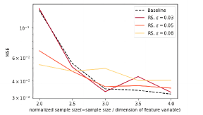
Figure 1 demonstrates how the RS model’s performance varies with different settings of the tolerate rate and across various sample sizes. For smaller sample sizes, the RS model outperforms the baseline that does not incorporate robustness; among those RS models, those configured with a larger (indicating a greater emphasis on robustness) perform better. This result notes the importance of accounting for robustness, particularly when there is a notable gap between the sampling and empirical distributions in small-sample regimes. As the sample size increases, the relative benefit of the RS model decreases. This trend is expected since a larger dataset allows to better picture the sampling distribution, making the baseline approach of empirical risk minimization increasingly effective.
5.2 RS Performance under Distribution Shift
We now evaluate the performance of RS under distribution shift. Let the model parameter in the sampling distribution be , and the model parameter in the target distribution be:
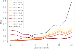
where Degree is a positive number characterizing the degree of distribution shift444Here our focus is on evaluating robustness in scenarios with smoothed parameters, rather than under arbitrary perturbations of . This setup is based on the observation that both DRO and RS, known for their robustness, typically yield smoother parameters than those derived from direct empirical risk minimization. . As Degree increases, the discrepancy between and increases, leading to a larger distribution shift between the sampling distribution and the target distribution .
Figure 2 shows how the RS model performs when configured with different tolerance rates and under various distribution shifts. For minor distribution shifts (Degree less than ), the RS model’s performance is comparable to the baseline, deteriorating slightly at models of larger for stronger robustness control. However, with more substantial distribution shifts (Degree greater than ), the RS model almost consistently outperforms the baseline, presenting stronger robustness under larger distribution shifts. This result highlights the potential of RS framework for strong generalization guarantee in uncertain environments.
5.3 Connection to DRO under Lipschitz loss
We proceed to compare RS and DRO. We establish explicit correspondence between the hyperparameters of RS and DRO in this type of problem. And we conduct experiments to compare their sensitivities to hyperparameter tuning.
5.3.1 Hyperparameter correspondence
Consider a Lipschitz loss function . We reformulate the general Lipschitz-loss learning problem following the DRO literature (Blanchet et al., 2019; Shafieezadeh-Abadeh et al., 2019):
| (17) |
Building on the reformulation presented in Section 2.2, this Lipschitz-loss learning problem under the RS framework is equivalent to:
| (18) | ||||
| s.t. |
By applying the Lagrangian method to solve Equation (18) and with the strong duality held, we further deduce that Equation (18) simplifies to the following expression (see Section C.1 for the proof):
| (19) |
We immediately observe a clear link between RS and DRO for the general Lipschitz-loss learning problem: given a reference value , solving the RS model (19) yields the optimizer . Then, by setting the radius in the DRO model (17) to , the DRO model (17) generates the same optimizer for the model parameter . Recall that the reference value is set to be throughout this paper, where is the tolerate rate that controls the robustness of RS. Thus each hyperparameter in the RS model is associated with a specific radius , the hyperparameter in the DRO model.

Figure 3 illustrates the relationship between the robustness-controlling hyperparameters of the two models: the DRO radius and the RS torelance rate . Notably, the function is concave with respect to , flatting as nears . This indicates that, to achieve comparable performance, the RS model can accommodate larger variations in compared to variations in for the DRO model, implying that RS is less sensitive to hyperparameter tuning. This observation will be further supported by the following experiments.
5.3.2 Numerical sensitivity analysis
We now conduct experiments to evaluate the sensitivity of RS and DRO to hyperparameter tuning. Specifically, we vary the tolerance rate in the RS model and the radius in the DRO model. We set the model parameter in the sampling distribution to , as in Section 5.2; and set the target environment to be .
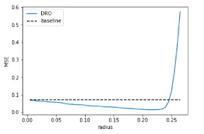

Figure 5 shows that DRO outperforms the baseline for radius smaller than , with the optimal around . Figure 5 shows that RS exceeds the baseline when is below , with the optimal around . The smallest MSEs from both DRO and RS models are comparable.
However, there is a drastic MSE surge in response to changes of for DRO in Figure 5, in contrast to the milder variation of MSE to for RS showed in Figure 5. This difference in hyperparameter sensitivity aligns with the nuanced relationship between and depicted in Figure 3. In particular, within a 15% relative error range around the optimal hyperparameters, the MSE for DRO may spike to , whereas RS maintains a more stable MSE of . This suggests that RS offers greater flexibility in setting the tolerate rate hyperparameter , unlike DRO, which requires more precise tuning for the radius .
6 Conclusions
This paper focuses on exploring the statistical properties of the RS model, a recent robust optimization framework introduced in (Long et al., 2023). We provide theoretical guarantees for the RS model, including two-sided confidence intervals for the optimal loss and finite-sample generalization error bounds. These guarantees extend to scenarios involving distribution shifts, highlighting the RS model’s robust generalization performance. Our numerical experiments reveal the superiority of the RS model compared to the baseline empirical risk minimization method, particularly in small-sample regimes and under distribution shifts. We establish explicit connections between the RS and DRO frameworks within specific models, showcasing that RS exhibits lower sensitivity to hyperparameter tuning than DRO, making it a more practical and interpretable choice. Future research directions include extending our analysis of RS to other distribution distances such as -divergence, proving lower bounds for generalization error, and applying RS to various practical applications.
Acknowledgement
We would like to thank the reviewers for their constructive feedback, which has greatly improved the current version of our work. Yunbei Xu acknowledges support from ARO through award W911NF-21-1-0328 and from the Simons Foundation and NSF through award DMS-2031883. Ruohan Zhan is partly supported by the Guangdong Provincial Key Laboratory of Mathematical Foundations for Artificial Intelligence (2023B1212010001) and the Project of Hetao Shenzhen-Hong Kong Science and Technology Innovation Cooperation Zone (HZQB-KCZYB-2020083).
Impact Statement
This paper presents work whose goal is to advance the field of Machine Learning. There are many potential societal consequences of our work, none which we feel must be specifically highlighted here.
References
- Bayraksan & Love (2015) Bayraksan, G. and Love, D. K. Data-driven stochastic programming using phi-divergences. In The operations research revolution, pp. 1–19. INFORMS, 2015.
- Blanchet & Murthy (2019) Blanchet, J. and Murthy, K. Quantifying distributional model risk via optimal transport. Mathematics of Operations Research, 44(2):565–600, 2019.
- Blanchet et al. (2019) Blanchet, J., Kang, Y., and Murthy, K. Robust wasserstein profile inference and applications to machine learning. Journal of Applied Probability, 56(3):830–857, 2019.
- Blanchet et al. (2021) Blanchet, J., Murthy, K., and Nguyen, V. A. Statistical analysis of wasserstein distributionally robust estimators. In Tutorials in Operations Research: Emerging Optimization Methods and Modeling Techniques with Applications, pp. 227–254. INFORMS, 2021.
- Chen & Chen (2023) Chen, S. and Chen, Y. Designing a resilient supply chain network under ambiguous information and disruption risk. Computers & Chemical Engineering, 179:108428, 2023.
- Deng et al. (2023) Deng, M., Bian, B., Zhou, Y., and Ding, J. Distributionally robust production and replenishment problem for hydrogen supply chains. Transportation Research Part E: Logistics and Transportation Review, 179:103293, 2023.
- Duchi et al. (2021) Duchi, J. C., Glynn, P. W., and Namkoong, H. Statistics of robust optimization: A generalized empirical likelihood approach. Mathematics of Operations Research, 46(3):946–969, 2021.
- Esfahani & Kuhn (2015) Esfahani, P. M. and Kuhn, D. Data-driven distributionally robust optimization using the wasserstein metric: Performance guarantees and tractable reformulations. arXiv preprint arXiv:1505.05116, 2015.
- Fournier & Guillin (2015) Fournier, N. and Guillin, A. On the rate of convergence in wasserstein distance of the empirical measure. Probability theory and related fields, 162(3-4):707–738, 2015.
- Gao & Kleywegt (2023) Gao, R. and Kleywegt, A. Distributionally robust stochastic optimization with wasserstein distance. Mathematics of Operations Research, 48(2):603–655, 2023.
- Hu & Hong (2013) Hu, Z. and Hong, L. J. Kullback-leibler divergence constrained distributionally robust optimization. Available at Optimization Online, 1(2):9, 2013.
- Huang et al. (2023) Huang, H., Li, Z., Gooi, H. B., Qiu, H., Zhang, X., Lv, C., Liang, R., and Gong, D. Distributionally robust energy-transportation coordination in coal mine integrated energy systems. Applied Energy, 333:120577, 2023.
- Kantorovich & Rubinshtein (1958) Kantorovich, L. V. and Rubinshtein, S. On a space of totally additive functions. Vestnik of the St. Petersburg University: Mathematics, 13(7):52–59, 1958.
- Kuhn et al. (2019) Kuhn, D., Esfahani, P. M., Nguyen, V. A., and Shafieezadeh-Abadeh, S. Wasserstein distributionally robust optimization: Theory and applications in machine learning. In Operations research & management science in the age of analytics, pp. 130–166. Informs, 2019.
- Lempert et al. (2006) Lempert, R. J., Groves, D. G., Popper, S. W., and Bankes, S. C. A general, analytic method for generating robust strategies and narrative scenarios. Management science, 52(4):514–528, 2006.
- Li et al. (2023) Li, Y., Han, M., Shahidehpour, M., Li, J., and Long, C. Data-driven distributionally robust scheduling of community integrated energy systems with uncertain renewable generations considering integrated demand response. Applied Energy, 335:120749, 2023.
- Liu et al. (2023) Liu, F., Chen, Z., and Wang, S. Globalized distributionally robust counterpart. INFORMS Journal on Computing, 2023.
- Long et al. (2023) Long, D. Z., Sim, M., and Zhou, M. Robust satisficing. Operations Research, 71(1):61–82, 2023.
- Mogensen & Thorstad (2022) Mogensen, A. L. and Thorstad, D. Tough enough? robust satisficing as a decision norm for long-term policy analysis. Synthese, 200(1):36, 2022.
- Rahimian & Mehrotra (2022) Rahimian, H. and Mehrotra, S. Frameworks and results in distributionally robust optimization. Open Journal of Mathematical Optimization, 3:1–85, 2022.
- Ronchetti (2021) Ronchetti, E. The main contributions of robust statistics to statistical science and a new challenge. Metron, 79(2):127–135, 2021.
- Ruan et al. (2023) Ruan, H., Zhou, S., Chen, Z., and Ho, C. P. Robust satisficing mdps. In International Conference on Machine Learning, pp. 29232–29258. PMLR, 2023.
- Saday et al. (2023) Saday, A., Yıldırım, Y. C., and Tekin, C. Robust bayesian satisficing. arXiv preprint arXiv:2308.08291, 2023.
- Shafieezadeh-Abadeh et al. (2019) Shafieezadeh-Abadeh, S., Kuhn, D., and Esfahani, P. M. Regularization via mass transportation. Journal of Machine Learning Research, 20(103):1–68, 2019.
- Sim (2023) Sim, M. The analytics of robust satisficing: predict, optimize, satisfice, then fortify. In Book of Abstracts, pp. 42, 2023.
- Sim et al. (2021) Sim, M., Zhao, L., and Zhou, M. Tractable robust supervised learning models. Available at SSRN 3981205, 2021.
- Wang et al. (2023) Wang, D., Yang, K., and Yang, L. Risk-averse two-stage distributionally robust optimisation for logistics planning in disaster relief management. International Journal of Production Research, 61(2):668–691, 2023.
Appendix A Key Propositions
Proposition 1.
For any distributions , , we have
| (20) |
where denotes the space of all Lipschitz functions with and is a norm
This is the dual representation of Wasserstein distance, and it needs the Assumption 2.
We will also utilize the bound of Wasserstein distance between and , which is presented below.
Appendix B Proof of Lemmas and Theorems
B.1 Proof of Lemma 1.
Choose , we have
| (21) |
Moreover, by the definition of , for any , we can choose one distribution , which satisfies:
| (22) |
Then (22) minus (21), we have:
| (23) | ||||
| (24) | ||||
| (25) |
for all and , Where the second inequality utilizes (20). Due to the arbitrariness of , we can ignore the terms of and choose as in (23), we get:
| (26) |
If , we will complete the proof.
B.2 Proof of Theorem 1.
For the right side , , where the second inequality is derived from the model (2) itself and the fact that .
For the other side, by the definition of , for any , choose satisfies:
| (27) |
Then
| (28) | ||||
| (29) | ||||
| (30) | ||||
| (31) |
for all . The second inequality is derived from (20) and the third inequality uses (27). Due to the arbitrariness of , we have , which can be solved:
Then we denote events . Then . Because , we use Borel-Cantelli Lemma and the limit supremum of the sequence of events satisfies:
| (33) |
So , which implies the consistency.
Finally, if , we can take and obtain (3.1).
B.3 Proof of Theorem 3.
B.4 Proof of Theorem 5.
The proof here is very straightforward following the proof of Theorem 1 and 3. Combine with the formula (12) that was proven earlier, we can easily obtain similar result:
| (34) |
Then we use the triangle inequality of distance: and we get the extra term . And for the term , continue to use the tail probability (2) to get guarantees for various probabilities and expected values.
Appendix C Supplementary results for Section 5
C.1 Derivation of Equivalent Models in Section 5.1
Proof of (17). For convenience, let denote the augmented parameter vector . Consider Lipschitz loss . For DRO, under mild assumptions, Esfahani & Kuhn have shown that:
| (35) |
Next, denote , Utilizing the proof given by Shafieezadeh-Abadeh et al., we can obtain:
The second equality here utilizes the definition of our fine-tuned cost function: if in and in are not equal, the distance will become , thereby making the entire expression . Therefore, only the distance of the feature variable is retained.
Back to (35), we have:
Then we have
| (36) |
Proof of (18). We have already given the reformulation of the RS model(7) in Section 2.2. The constraint condition is:
| (37) |
The proof will follow the proof of (17):
Since serves as the upper bound in (37), to ensure that the left side of (37) is not infinite, it is necessary to satisfy . Therefore, in (7), taking the minimum value of is equivalent to minimizing and let , while satisfying the constraint condition .
Proof of (19). Following (18), we can express it in its dual form:
Notably, this equation represents a convex problem. As long as which is mentioned in (4), there exists a point in the relative interior, hence the Slater’s strong duality condition holds. Subsequently, to facilitate comparative analysis with DRO, we replace with to obtain:
Finally, note that the above equation is convex with respect to and concave with respect to . According to the Mini-max theorem, we can interchange the order of sup and inf to obtain the desired formula.
C.2 Other Equivalent Conclusions
This section answers the question mentioned in the previous footnote. If we still use the norm of the entire vector as the cost function i.e. , then the DRO model will be equivalent to:
where is the augmented vector . Similarly, RS model is equilvalent to:
| s.t. |
And we can also write its dual equivalent form as:
Therefore, after modifying the definition of the cost function, the only difference is whether one term in the model is the norm of the parameter itself or the norm of the augmented vector obtained by adding an element .
C.3 Function in Ten Dimensions
In Section 5.1, we set the feature variable to be ten-dimensional. As a supplement to Section 5.2 , we also plot the relationship graph under the ten-dimensional situation of the feature variable.
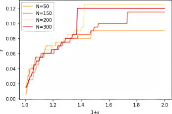
Figure 6 shows similar relationship between the robustness-controlling hyperparameters of the two models: the DRO radius and the RS tolerance rate . The overall trend of the graph is concave. It tends to flatten when . Moreover, when the function tends to be flat, the corresponding radius value is smaller than that in the two-dimensional case in Figure 3.
Appendix D Some Classical Loss Functions
Here we present a few common loss functions.
| L(z) | Classification(C) or Regression(R) | Learning Model | |
|---|---|---|---|
| Hinge Loss | C | SVM | |
| Smooth Hinge Loss | C | smooth SVM | |
| Logloss | C | Logistic Regression | |
| Squared Loss | R | MSE | |
| Loss | R | MAE | |
| Huber Loss | R | Huber regression | |
| -insensitive Loss | R | support vector regression | |
| Pinball Loss | R | Quantile regression |
Here we consider as a loss function for machine learning applications, where denotes the parameters in the classification or regression model, and represents the data with as the feature variable and as the label variable. For binary classification problems, the loss function can be defined as follows:
| (38) |
For regression problems, the loss function can be defined as follows:
| (39) |
Here we present a few common loss functions (See Table 2). Apart from the squared loss, all other loss functions in Table 2 are Lipschitz, so our Assumption 2 is relatively weak and reasonable. Furthermore, in practical applications, and are often bounded, so even if we use squared loss, it is Lipschitz in the case of a bounded domain.
Appendix E Discussion on Lipschitz continuity Assumption
In our paper, we do not need to assume the Lipschitz continuity of the loss function with respect to , but with respect to . This assumption follows that of (Esfahani & Kuhn, 2015), with the aim of using the inequality in Proposition 1. We however understand that it is a common condition to assume the Lipschitz continuity of parameter . In response to this, we provide a conservative answer: at least for the regression problem in Appendix D where , if both the random variable space and the parameter space are bounded, then as long as we assume that is a Lipschitz function, it can be simultaneously derived that is Lipschitz with respect to both and . In such scenarios, the Lipschitz assumptions for and hold simultaneously.