Algorithmic Fairness in Performative Policy Learning: Escaping the Impossibility of Group Fairness
Abstract.
In many prediction problems, the predictive model affects the distribution of the prediction target. This phenomenon is known as performativity and is often caused by the behavior of individuals with vested interests in the outcome of the predictive model. Although performativity is generally problematic because it manifests as distribution shifts, we develop algorithmic fairness practices that leverage performativity to achieve stronger group fairness guarantees in social classification problems (compared to what is achievable in non-performative settings). In particular, we leverage the policymaker’s ability to steer the population to remedy inequities in the long term. A crucial benefit of this approach is that it is possible to resolve the incompatibilities between conflicting group fairness definitions.
1. Introduction
Automated decision-making and support systems that rely on predictive models are often used to make consequential decisions in criminal justice (Rudin, 2013; Casselman and Goldstein, 2015), lending (Petrasic et al., 2017), and healthcare (Deo, 2015), but their long-term impacts on the population are poorly understood. Most prior work on algorithmic fairness assumes a static population and focuses on allocative equality (Crawford, 2017). For example, consider the common fairness definition equalized odds (Hardt et al., 2016b). It requires a predictive model to incur false positives and false negatives at equal rates across demographic groups; i.e. it requires the model to allocate errors equally between groups. It does not consider long-term impacts of errors across demographic groups: for example, it may be easier for members of an advantaged group to overturn an error (as compared to members of a disadvantaged group), so errors are more consequential for the disadvantaged group. In the long term, this can exacerbate inequalities in the population in ways that simply enforcing equalized odds cannot address.
Motivated by concerns about the long-term impacts of predictive models, there is a line of work that embeds predictive models as policies in dynamic models of populations and studies how predictive models steer the population (Heidari et al., 2019; Kannan et al., 2019; D’Amour et al., 2020; Yin et al., 2023). Following this line of work, we study the enforcement of group fairness in the long term. Our contributions are as follows.
- (1)
-
(2)
We show that as long as the policymaker has enough flexibility in the way they remedy historical inequities, it is possible for them to steer populations towards a reformed state while maintaining group fairness. As a consequence, this shows that it is possible, in the long term, to simultaneously satisfy traditionally conflicting group fairness constraints.
-
(3)
We provide a reduction framework for computationally enforcing long-term group fairness. The convergence rates and generalization guarantees of this framework are provided.
As mentioned, a key consequence of our results is that in the long term, it is possible to simultaneously remedy historical disparities and satisfy multiple group fairness definitions that are traditionally incompatible. This is in contrast to previous research on compatible group fairness. The common theme of previous work is that of avoidance, i.e. practitioners should alter policies so that the different notions of fairness are fully satisfied at separate times or relaxed versions of group fairness are satisfied simultaneously. Instead, our focus is on resolution of incompatibility of group fairness, i.e. practitioners should implement policies that eliminate the inequity that leads to the impossibility of enforcing multiple forms of group fairness.
1.1. Related Work
We first cover the prior work on resolving group fairness incompatibilities, this is a non-exhaustive list and a thorough survey is given in (Raghavan, 2023). The study of incompatibilities in group fairness was initiated simultaneously by the impossibility results in the works (Kleinberg et al., 2016; Chouldechova, 2017). In the years since then, researchers have sought to extend these results and modify fairness practices to partially resolve them. The work (Berk et al., 2017) covers impossibility results for several group fairness metrics derived from confusion matrices in the context of recidivism. Beyond just group fairness, trade-offs between optimal accuracy, fairness, and resource allocation for different groups have also been explored (Pleiss et al., 2017; Donahue and Kleinberg, 2020). The line of work (Lazar Reich and Vijaykumar, 2021; Madras et al., 2018; Canetti et al., 2019) studies algorithmic fairness in ML systems with human elements, although ultimately the aggregate decision making process (human plus machine) is still burdened by impossibility theorems. Another avenue of approach is to relax the sufficiency and separation requirements to compatibility (Pleiss et al., 2017; Celis et al., 2019; Gultchin et al., 2022; Lohaus et al., 2020; Padh et al., 2021), although direct trade-offs between fairness notions remain, and often such relaxations do not guarantee a desired level of fairness. Philosophically, our work aligns with the recent idea of substantive fairness, which argues that policies should aim to eliminate historical inequities, treating causes of disparity rather than symptoms of disparity (Davis et al., 2021; Green, 2022). One of the main contributions of this work is to formalize substantive fairness into an algorithmic framework and study the feasibility of erasing historical disparities with ML systems.
Concern amongst the fairness community regarding the long-term impacts of predictive models has grown, originating with a line of work that models fair policies and populations as a dynamical system(Heidari et al., 2019; Kannan et al., 2019; D’Amour et al., 2020). The long-term fairness framework that we study is based on the recently developed idea of performative prediction, a line of work that studies model-induced distribution shift (Perdomo et al., 2020; Mendler-Dünner et al., 2020, 2022; Brown et al., 2022; Izzo et al., 2021). Closely related lines of work on the enforcement of fairness in performative settings include (Rateike et al., 2023; Zezulka and Genin, 2023; Yin et al., 2023). The work (Rateike et al., 2023) designs a Markov chain oriented framework of performative fairness, while the work (Yin et al., 2023) develops algorithms that minimize cumulative fairness regret in online settings. These generally consider a stateful performative prediction setting and cast the task of steering the underlying dynamical system as an optimal control or reinforcement learning problem. In contrast, our problem setting prioritizes the discrimination in the steady state and is not concerned with intermediate time steps. Finally, the authors of (Zezulka and Genin, 2023) propose procedures for estimating discriminatory outcomes of policies.
Although it predates performative prediction, strategic classification (Hardt et al., 2016a) is a common example of performative prediction. As such, attention has been paid to the study of fairness in strategic settings. The authors of (Estornell et al., 2023b) show that traditional fairness interventions in strategic settings can actually exacerbate discrimination. A similar perspective on traditional fairness constraints in strategic settings is given in (Liu et al., 2018). In (Zhang et al., 2022) the effect of fairness interventions on the incentive for strategic manipulation is studied. The work (Hu et al., 2019) shows that cost discrimination in strategic classification will cause violations of group fairness constraints in the long term. The authors of (Liu et al., 2020) also study cost discrimination in strategic classification, showing that subsidies for the disadvantaged group can alleviate discrimination concerns. The common goal for each of these works (and others in this area) is to study how strategic interventions make discrimination worse if either no fairness intervention is used or if a *traditional* fairness intervention (that does not account for strategic agents) is used. The key difference between this line of work and our work is that this line of work considers strategic behavior as a problem to be overcome, while we leverage strategic behavior for greater fairness achievement than is possible in non-strategic environments.
The running example of performative prediction/ a strategic setting in this paper is labor market models; the study of such models has a rich history in economics and long precedes the idea of performative prediction. A comprehensive survey of this field is given in (Fang and Moro, 2011). The works (Arrow, 1971; Phelps, 1972) presented initial labor market models and analyzed the equilibrium of these models at the worker level. In (Phelps, 1972), discrimination in labor markets due to exogenous groups is studied, while (Arrow, 1971) surprisingly shows that even markets with endogenous groups will have discriminatory equilibrium. Later, the authors (Coate and Loury, 1993) formulated these ideas in the celebrated Coate and Loury model of labor markets. Extensions on this model are numerous; the authors of (Moro and Norman, 2004) and (Moro and Norman, 2003) develop a model where wages are set by inter-employer competition and groups of workers actually benefit from discrimination of others. The line of work (Fryar et al., 2008; Fryar and Loury, 2005, 2013; Craig and Fryer, 2017) studies the efficacy of color-blind policies in preventing discrimination. We will primarily work with our own models of labor markets, inspired by (Somerstep et al., 2024; Shavit et al., 2020).
Our primary goal is to study the feasibility of (fairly) equating response distributions between two groups in the long term. This is closely related to the goal of incentivizing agents to improve some desirable quality. The authors of (Miller et al., 2020) show that this involves causal modeling, and our work is no exception: various labor market models will play the role of the causal model in our study. The works (Milli et al., 2019; Somerstep et al., 2024) focus on improving the agents’ overall welfare; they show that there is often a trade-off between the learner and the agents’ utilities. Performative power (Hardt et al., 2022) measures the ability of the learner to steer the agents in performative prediction. As we shall see, the firm in the aforementioned labor market models possess enough performative power to equate ex post response distributions despite ex ante disparities between the two groups. Finally, the causal strategic labor market model that we develop is an example of an outcome performativity problem. outcome performativity is introduced in (Kim and Perdomo, 2023) along with efficient omniprediction algorithms for outcome performativity problems. In general, the novelty of our work is our focus on a) driving improvement with the goal of equating disparate groups and b) doing so without discriminating against the advantaged group.
2. Group fairness in performative policy learning
Consider a binary classification problem in which samples correspond to a population of individuals invested in learned policies (often referred to as strategic agents) characterized by and a protected attribute denoted . This setting is characterized as a problem in performative prediction. Performative prediction is a distribution shift setting, where the implementation of a policy triggers responses from the individuals invested in the policy, leading to a new distribution of data . Throughout, we will assume that group proportions remain constant (say ) for any policy . Under this assumption, we can write
| (2.1) |
In performative prediction, The policy maker’s goal is to make a policy that maximizes their expected reward, taking into account the strategic response of the individuals to their decisions:
| (2.2) |
where is a policy class, is the distribution map that encodes the long-term impacts of the policy on the subset of the population with sensitive trait value , is the policy maker’s reward function that measures their reward from applying a policy to an agent (this agent also has group membership ), and is the proportion of the population with sensitive trait value . The objective function in (2.2) is often called the performative (expected) utility and measures the ex post reward of policies. Throughout this paper, we will mark random variables drawn from an ex post distribution as .
A recurring instance of performative policy learning in this work is the hiring firm’s problem in Coate-Loury-type models of labor markets (Fang and Moro, 2011).
Example 2.1 (Continuous labor market example (Somerstep et al., 2023)).
Consider an employer that wants to hire skilled workers who reside in one of two identifiable groups . The workers are represented as quintuples. is a worker’s (latent) base skill level, a workers productivity and be a noisy productivity assessment (e.g. the outcome of an interview). Throughout, it is assumed that conditioned on , productivity is independent of and that
The productivity assessment is independent of given and specified by a conditional CDF
that decreases in (at a fixed ). We note that this also specifies the generation of as
Intuitively, the assumption that decreases in at a fixed , requires the productivity assessment to be “unbiased” (in the sense of a statistical test). Under this unbiased assumption, the optimal hiring policy for the firm is of the form . Let be the firm’s received utility from hiring () or not hiring () a worker with productivity . The firm’s expected utility for policy is , so the firm’s utility maximization problem is
As in (Coate and Loury, 1993), we allow the workers to improve their skills (at a cost) in response to the firm’s policy. Let be the wage paid to hired workers and be the sensitive trait dependent cost to workers of improving their skills from to . We assume is non-increasing in and non-decreasing in . The expected utility a worker with group membership receives from increasing their skill level from to is
so a strategic worker changes their skill level to maximize their expected utility. We encode the ex-post workers’ skill level, skill level assessment, and productivity as
Note that the (conditional) distribution of a worker’s skill level assessment, given their skill level, remains the same before and after the worker changes their skill level. To account for the strategic behavior of the workers, the firm solves the performative policy learning problem:
The workers do not respond instantly to the employer’s hiring policy; it takes them a while. Thus, we interpret as the long term distribution of the workers’ skill levels and assessments in response to the employer’s hiring policy. More concretely, imagine a labor market in which the workers slowly turn over: new workers enter the workforce and old workers retire constantly. As workers enter the workforce, they make their human capital investment decisions in response to the employer’s (contemporaneous) hiring policy. Over a long period, the labor force population will converge to .
2.1. Standard fairness constraints are insufficient in performative prediction
The standard way to enforce fairness in policy learning problems is to equalize certain fairness metrics between demographic groups (indicated by a demographic attribute ). This is often done by imposing fairness constraints on the policy learning problem. In general, fairness constraints fall into one of three types:
| (demographic parity DP) | ||||
| (separation) | ||||
| (sufficiency) |
To see each of the traditional group fairness constraints in action, consider example 2.1. Enforcing separation requires identical ex-ante hiring rates between workers from the advantaged and disadvantaged groups with the same skill level, while enforcing sufficiency requires the ex-ante (distribution of) skill levels of the hired workers from the majority and minority groups to be the same. Finally, enforcing demographic parity simply requires that the ex-ante hiring rites for individuals be the same across the groups.
In the long-term setting, there are two main issues with such group fairness constraints. First, they only focus on the policy and not its long-term impacts on the population: the policy appears in all three constraints, but the distribution map that encodes the long-term impacts of is absent. In other words, group fairness constraints enforce equal treatment, but ignore the long-term impacts of equal treatment on the population. Consider example 2.1, only ex-ante quantities of the workers are considered. This leads us to consider constraints that focus on the long-term impacts of the policy on the population. Instead of enforcing ex-ante equal treatment, we seek ex-post equality of certain fairness metrics.
Second, traditional group fairness constraints are also plagued by incompatibilities. Despite the intuitive nature of DP, separation and sufficiency, (Chouldechova, 2017; Kleinberg et al., 2016) prove that it is generally impossible for a policy to simultaneously satisfy two of DP, separation and sufficiency.
Theorem 2.2 (Chouldechova (2017); Kleinberg et al. (2016)).
It is impossible to find a joint distribution on that satisfies two of DP, separation, and sufficiency, unless one of the following hold:
-
(1)
-
(2)
This result is generally interpreted as an impossibility result: it is impossible to simultaneously satisfy separation and sufficiency. Although there are two cases in which separation and sufficiency are compatible, they are considered pathological. The first case, perfect prediction, is generally unachievable because the Bayes error rate in most practical prediction problems is non-zero. The second case, independent responses, is also considered pathological because the policymaker has no control over the distribution of responses. However, in performative settings, the policymaker can steer the population so that response distributions are equal, suggesting that it is possible to resolve the incompatibilities between separation and sufficiency in performative settings by enforcing group-independent responses ex-post. In the next section, we build on this observation to resolve the incompatibility between separation, sufficiency, and demographic parity in performative settings.
2.2. Equality of Outcomes
The preceding developments suggest that the goal of a fairness-conscious policymaker should be to eliminate disparities between demographic groups in the long term (instead of myopically enforcing group fairness regardless of the long term impacts). Because we are interested in equating the different demographic groups ex-post (where an individual from each group ends up) rather than equating the different demographic groups ex-ante (where an individual from each group comes from), we refer to this constraint as equality of outcomes.
Definition 2.3 (Equality of outcomes).
A policy satisfies equality of outcomes with respect to metric if and only if is constant over each possible value of the sensitive trait .
We emphasize that fairness metrics are not metrics in the distance sense, but rather a quantity that measures a long-term outcome of interest for strategic individuals. Since we are interested in ex-post fairness, each metric will measure quantities associated with the ex-post distribution (). Finally, for simplicity of presentation, we will present each metric for the case of binary classification . The extension to the multiclass or continuous case is straightforward.
The goal of algorithmic reform in example 2.1 is to equalize the disparities in human capital investment among minority and majority workers. Choosing the fairness metric in definition 2.3 to be worker productivity, we can encode this goal as an instance of definition 2.3.
Definition 2.4 (equality of responses).
A policy satisfies equality of responses if it satisfies equality of outcomes with respect to the metric .
Equal responses is a concept of fairness unique to the long-term setting (and is our interpretation of the aim of algorithmic reform/reparation); we note that it does not imply the long-term analog of group fairness defined next. We opt to refer to equality of outcomes with respect to any metric containing the policy as equality of treatment.
Definition 2.5 (Equality of treatment).
A policy satisfies equality of treatment if meets all the following criteria.
-
(1)
The policy satisfies equality of outcomes with respect to metric .
-
(2)
The policy satisfies equality of outcomes with respect to both metrics
-
(3)
The policy satisfies equality of outcomes with respect to both metrics
We we wish to emphasize that requirements one, two and three are simply the long term analogs of demographic parity, separation and sufficiency respectively. Thus, the enforcement of equality of treatment implies the long-term enforcement of multiple fairness constraints that are incompatible in the short term.
Of course, our ultimate goal is for policymakers to implement policies that satisfy equality of responses and equality of treatment simultaneously. We point out that these goals are not necessarily disjoint. As previous impossibility theorems have shown, in most cases satisfying equality of responses is a prerequisite to satisfying equality of treatment. We show in the following proposition that satisfying equality of treatment and equality of responses is equivalent to enforcing the independence of the joint distribution and .
Proposition 2.6.
A policy satisfies equality of treatment and equality of responses if and only if the joint distribution is independent of .
As mentioned, equality of responses is a mathematical formalization of the line of work on algorithmic reform/reparation (Davis et al., 2021; Green, 2022). This line of work “escapes” from incompatibilities between group fairness definitions by questioning the goal of satisfying those definitions. It argues that the underlying goal of enforcing fairness is to remedy injustices. From this perspective, traditional algorithmic fairness definitions are merely a flawed indicator of the true goal, so it is inconsequential if they are incompatible. We encode the goal of reform or reparation mathematically as closing or eliminating disparities in the responses of interest among demographic groups. Furthermore, we study the enforcement of equality of responses and equality of treatment simultaneously. In our formulation, this implies the attainment of algorithmic reform/reparation without discrimination. In (Davis et al., 2021; Green, 2022), it is often argued that reform can only be achieved by discriminating against the advantaged group. In contrast to this, our analysis will show that it is often possible to achieve reform (equality of responses) fairly (equality of treatment).
3. Feasibility of equality of outcomes
A crucial and non-trivial question remains. Is it feasible to enforce equality of treatment and equality of responses simultaneously? Note that this requires the same policy to equate ex-post responses and to satisfy equality of outcomes with respect to each long-term group fairness metric. If we deploy one policy to steer the population so that the response distributions are equal and another policy to satisfy the equality of treatment constraints, the second policy may steer the population away from equated responses, and we end up in a cycle that achieves neither goal. Unfortunately, the goal of equal responses and equal treatment may not be possible, even in performative settings; i.e. there may not be a policy that achieves both the treatment and the response goals. This is because the distribution map depends on the sensitive attributes (e.g. because it encodes inequities in the ex-ante distribution or inequities in the agent response map). Thus, equating the responses ex-post requires disparate treatment of the group (i.e. the policymaker cannot simply implement the same policy for each group). On the other hand, equality of treatment forbids a disparate allocation of ex-post errors between groups. In this section, we study the feasibility of enforcing equality of treatment (and thus equality of responses) in labor market models.
3.1. Impossibility Results
We start by establishing impossibility results to elucidate problem structures that preclude equality of treatment and equality of responses in labor market models. We consider two types of disparities: human capital investment cost disparities and ex-ante skill disparities. In order to introduce ex-ante skill disparities, we define the notion of stochastic dominance.
Definition 3.1 (stochastic dominance).
Consider two real valued random variables and . Then stochastically dominates if for all , .
We return to the continuous labor market model 2.1 in which an employer hires workers from two demographic groups. In order to keep the example as equitable as possible (so that it is as easy as possible for the employers to achieve equality of treatment), recall that we assume that the skill assessment process is fair () and the same wage is paid to hired workers from both groups. Thus, the only ex-ante differences allowed between workers in the two groups are the ex-ante distribution of their skill levels and the cost of human capital investment.
Theorem 3.2.
Assume the following:
-
(1)
The worker cost function is of the form , and is large enough to enforce strong convexity of the agents optimization problem
-
(2)
Exactly one of two forms of market discrimination is present:
-
(a)
There is a difference in ex-ante skill levels (specifically stochastically dominates ).
-
(b)
The is a difference in the cost of human capital investment of the form .
-
(a)
Then, under either form of discrimination, group-blind policies that ignore the demographic attribute of the workers cannot achieve equality of responses. Furthermore, hiring policies that satisfy equality of outcomes with respect to and are necessarily group-blind.
3.2. Alternative performative models
We present the preceding negative results to emphasize that simultaneously achieving equality of responses and equality of treatment with respect to various fairness metrics is not trivial. To overcome the difference ex-ante between workers in the two groups, employers must offer additional incentives to the ex-ante least skilled group to close the skill gap and achieve equal responses. Unfortunately, this prevents them from treating workers from the two groups equally because employers only have a single degree of freedom (the hiring threshold ). This suggests that it may be possible for employers with more degrees of freedom to equalize ex-post response distributions with an (ex-post) fair hiring policy.
In this section, we introduce two models, the first is a generic model of causal strategic classification inspired by the work (Shavit et al., 2020). The second is a modification of the causal strategic classification model to better model labor markets. The causal strategic classification model provides a simplified framework for theoretical questions on feasibility and generalization, while also demonstrating that our fairness framework is applicable to a wide variety of learning settings.
Example 3.3 (causal strategic classification (Shavit et al., 2020)).
Consider a learning setting, in which samples correspond to strategic agents that posses features and a sensitive trait . Conditioned on sensitive trait membership , features are generated from the ex-ante distribution
Conditioned on the features , the agent responses are generated via the Bernoulli variable
Note that this implies . The learner wishes to accurately classify the agents using the features and sensitive trait. As such, the learner deploys predictions generated with the model
In response to model choice , an agent (with trait and ex-ante features ) is allowed to take some action to improve their standing with the learner (at cost ). The agents act rationally, optimizing their utility:
Upon selecting action the agent’s features are ex-post . The matrix is an effort conversion matrix, encoding the improvement of the feature from the action for each .
At the population level, the ex-post feature distribution for the group is given by
Conditioned on and ex-post responses are generated by
and ex-post predictions are generated by
To prevent arbitrary inflation of all agent outcomes, the learner is subject to regularization penalty . From the above, the learners ex-post risk is
To better model a labor market, we modify example 3.3. The learning setting will correspond to a labor market and the strategic agents will correspond to workers. The key difference is that, rather than features, workers now have a profile of latent skills, and each skill contributes to the productivity of a worker. Consequently, firms now view a noisy measurement of each skill based on a factor model. This provides workers with multiple ways of investing in their human capital and firms with flexibility in their hiring policies. As we shall see, this additional flexibility is crucial for the enforcement of equality of treatment.
Example 3.4 (Modified Labor Market Model).
Consider the causal strategic classification set up (example 3.3). In the context of a labor market, the learner corresponds to a hiring firm, and each strategic agent is a worker. Workers are encoded by pairs , with corresponding to a latent skill profile; as before and we say . The productivity of the workers in the group is generated by . Rather than observing latent skill profiles, the hiring firm views interview outcomes generated by , with a matrix of factor loadings. This skill assessment model is motivated by item response theory (IRT) models of test outcomes (Lord, 1980). The results of the interviews are used to make hiring decisions through policy
A worker in group with an initial skill profile can take action (possibly training, studying, or additional education) in response to through the causal strategic classification response mechanism
The ex-post skill profiles are , which propagates to the ex-post interviews , productivity and hiring decisions . The firm seeks to maximize some (regularized) ex-post reward/profit
3.3. Feasibility of Equality of Treatment in Alternative Models
In contrast to the models in example 2.1, in the causal strategic classification setting (and the alternative labor market mode)l, the set of policies that enforces equality of treatments (and thus equality of responses by 2.6) is non-empty. In fact, it contains a stratified manifold of dimension , so the set is quite large in some sense. We will study this set in two scenarios: correcting ex-ante feature/skill disparities and correcting cost-of-improvement disparities. For the purposes of a theoretical analysis, we operate under some simplifying assumptions.
Assumption 3.5.
The quadratic cost assumption is standard in the strategic learning literature, (Shavit et al., 2020; Izzo et al., 2021; Jagadeesan et al., 2023). The effort matrix is of the form , if each skill is improved by a distinct action and only some skills can be improved. Each assumption (including normality) is primarily for mathematical convenience; we expect that feasibility will hold under a wide class of choices for and measures on .
Under assumption 3.5, the feasibility of equality of treatment can be studied by analyzing two disjoint constraint sets, one that pertains to parameters that correspond to “manipulable” features and another that pertains to “nonmanipulable” features, which we now define.
Definition 3.6 (Manipulable features).
Given an effort matrix , and a general feature vector , we let and be the manipulable and nonmanipulable features, respectively.
Additionally, we will assign , as the dimensions of the parameter spaces .
Theorem 3.7.
Consider the learning setting of example 3.3 with the minor assumption that the vectors are not co-linear, and the vectors are not co-linear. Suppose that one of the two following forms of discrimination is present:
-
(1)
Ex-ante distribution discrimination: , but ,
-
(2)
Cost of improvement discrimination: but .
Then under (1) or (2) there exist stratified manifolds , such that , and and any learner decision that satisfies and also satisfies equality of treatment and equality of responses.
Corollary 3.8.
Consider the modified labor market model (example 3.4). Assume that worker discrimination of the form (1) or (2) is present. Then if there exists a stratified manifold of dimension such that any satisfies equality of treatment.
Theorem 3.7 and corollary 3.8 state that in the causal strategic classification model/modified labor market model, the set of policies that enforce long-term fairness and correct differences in worker skills or costs contains a manifold of dimension . Here, is interpreted as the “number of skills” a worker can possess. This result clarifies the importance of flexibility in human capital investment. If is not large enough, then the feasible subsets of Theorem 3.7 will be either too small to provide policy makers flexibility or even empty in extreme cases. The assumptions of theorem 3.7 also provide an important form of policy maker flexibility; the existence of skills that are immune to performative effects implies the existence of policy parameters that can be adjusted to change error rates between groups without impacting downstream responses.
Open questions on the feasibility of equality of treatment in labor markets with multiple forms of discrimination or continuous outcomes remain. The assumption that only one form of discrimination is present (cost of education discrimination or ex-ante skill discrimination) is necessary for our analysis but not necessary for feasibility (see Figure 1(d) for a numerical example). The discrete nature of worker productivity and firm hiring decisions is also not strictly necessary; for example. The argument of theorem 3.7 immediately implies feasibility (assuming Gaussian features) in the Causal Strategic Least Squares model posited in (Shavit et al., 2020). This model is both the inspiration for our labor market model and can also be interpreted in the context of a labor market with continuous worker productivity.
4. A reduction algorithm for equality of outcomes
In practice, a policy maker often does not have complete knowledge of the ex-ante and ex-post distributions but instead only observes some samples from the ex-ante distribution and has some model for how individuals respond to their policy. We turn to the question of implementing equality of outcomes under such conditions, providing a reduction algorithm (inspired by Agarwal et al. (2018)) adapted to the performative setting. By proposition 2.6 a policy maker can implement equality of treatment and equality of responses by enforcing the independence of the joint distribution and . We propose that the policymaker enforce this through a series of moment inequality constraints:
Throughout this section, we will work with the causal strategic classification setting (example 3.3) in the two group setting. In this model, equal responses and equal treatment can be enforced through a series of 6 moment constraints.
Example 4.1.
Consider the causal strategic classification example 3.3 with two possible groups . In this setting, the condition is equivalent to the constraint:
while the ex-post risk is given by
The case of multi-class classification or multiple sensitive traits is relatively similar. For multiclass classification, enforcement of the independence requirement will require the addition of higher-order moment constraints, and moment constraints may simply be repeated for each possible sensitive trait combination in the case of multiple sensitive traits.
Recall that the policy maker is vested in minimizing some ex-post risk, therefore, in aggregate, the policymaker must solve a constrained optimization problem in . The primal problem is
| (4.1) |
In practice, the policymaker only observes samples from the ex-ante distribution. We will assume that the policymaker has access to some correctly specified model of at the sample level. For example, a hiring firm in a labor market would need to be aware of each worker’s cost-adjusted utility optimization problem. Using ex-ante samples and knowledge of , the policymaker can obtain the natural empirical estimates of and (denoted and ). As an example of obtaining estimates for and from we return to the modified labor market model.
Example 4.2 (Equality of outcomes estimates in causal strategic classification).
Recall the setting of Example 3.3. Consider an agent with sensitive trait and ex-ante features , upon viewing policy , the agent invests in their own features via Given an ex-ante sample of skill features from group , a reasonable choice of estimates for and are
After attaining estimates and , equation 4.1 can be replaced with said estimates. Furthermore, for convergence reasons, a norm constraint is placed on the dual variable . Finally, due to statistical error, a relaxation is allowed on the moment constraint. If the learner instead opts to solve the dual problem (the justification for this is expanded upon in Appendix A), the final result is
| (4.2) |
From here, the iterates of the dual variables are obtained using mirror ascent on the dual variable with the potential function , which algorithm 1 lays out explicitly.
Two elements of the algorithm 1, are nontrivial: (i) the -saddle point stopping criteria; (ii) the attainment of the best decision of the policy makers .
The -approximate saddle point stopping criteria: A primal dual pair is a -saddle point if the following hold:
Checking the first criteria reduces to a problem in attainment of the policy makers best decision (Agarwal et al., 2018). The second requirement requires solving a linear program with an L1 inequality constraint, a well-studied problem (Boyd and Vandenberghe, 2004).
Obtaining of the policymakers best decision : Attaining the best long-term policy for risk function is generally a nontrivial problem. Previous works have established methods for obtaining the best policy under the assumption that the policy maker knows the map (Horowitz and Rosenfeld, 2023; Levanon and Rosenfeld, 2021; Somerstep et al., 2024). Such methods are generally specific to a particular , and since our focus is on fairness, we will assume that the policymaker has access to some oracle which produces such an . This is a strong assumption, and our methodology is limited to performative maps that allow for such an oracle.
4.1. Algorithm 1 in the Modified Labor Market Model
As an application of Algorithm 1, we study the problem of enforcing equality of outcomes and equality of responses in the modified labor market (example 3.4) when both ex-ante distributions and cost of education are different between each group. We assume that , so that the firm has an unbiased estimate of each skill. Figure 1(d) demonstrates the performance of algorithm 1 on a held-out test set of workers. Prior work on long-term fairness studied the impact of enforcing standard fairness constraints in the long term, and, as such, we utilize this as a base line. Algorithm 1 is compared to policies that equalize one ex-ante fairness metric, including false positive rate, false negative rate, demographic parity, and sufficiency.
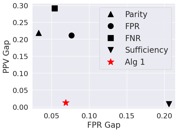
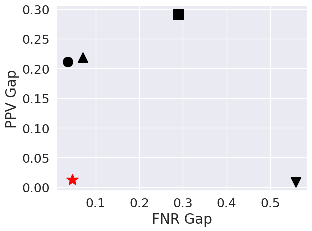
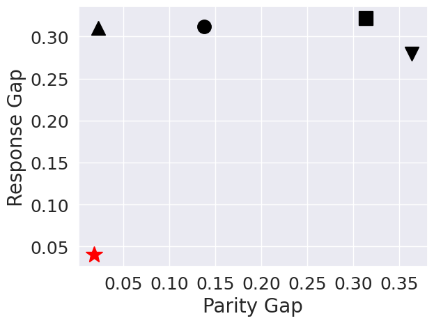
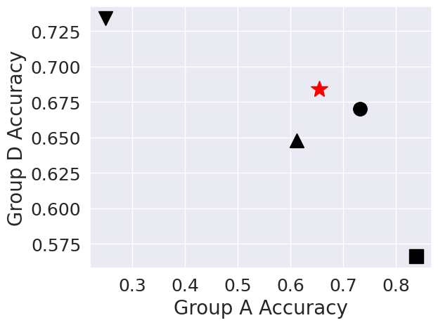
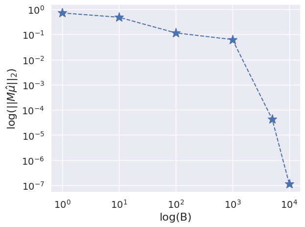
Figure 1(d) (a) and (b) demonstrate that in the long term sufficiency and separation are compatible, while figure 1(d) (c) shows that in the modified labor market model, a policymaker can satisfy equality of responses with a fair policy. Figure 1(d) (d) also demonstrates that enforcing equality of treatment and equality of responses will equate the error rate of a policy between the two groups. Due to statistical error (exacerbated by the opaque nature of worker skills), perfect fairness is not achieved on the test set. We emphasize that this is not due to an issue of feasibility, figure 2 demonstrates that algorithm 1 can attain nearly zero fairness violation on the training set.
5. Summary and discussion
In this paper, we studied fairness in performative settings in which the policymaker has the ability to steer the population. We showed that it is possible for the policymaker to remedy existing inequities in the population. In particular, we showed that by equating the distribution of responses between groups in classification problems, it is possible for the policymaker to simultaneously satisfy multiple notions of group fairness that are generally incompatible in non-performative settings. However, we also showed that this is not always possible: if the policymaker does not have enough flexibility in how they can equalize base rates, then it is unfortunately impossible, even in performative settings, to resolve the longstanding incompatibilities between group fairness definitions. Another limitation of our approach is that the policymaker must be aware of the long-term impacts of their policies on the population. Although this requirement is necessary, it limits the applicability of the approach. One possible direction for future work is to develop methods that help the policymaker estimate the effects of their policies on the population. Such methods can be combined with our approach to steer sociotechnical systems towards more equitable states.
Our work is also aligned with the goals of algorithmic reform/reparations. By considering reform/reparations mathematically, we show that it is somewhat possible to achieve the goals of reform without unequal treatment. This is especially desirable in application domains in which unequal treatment is illegal or impractical. For example, consider the problem of underrepresentation of women in the tech sector, especially in technical roles (Dastin, 2018). The authors of Davis et al. (2021) suggest that employers in the tech sector should adopt a “reparative” approach to equalize the representation of men and women, even if this entails explicitly discriminating against men. They justify explicit discrimination by appealing to the historical injustices that led to the dearth of women in the tech sector and the need to remedy such injustices. Although a discriminatory approach is likely to be limited by various labor laws, our results suggest that it may be possible to equalize the representation of men and women while treating men and women fairly. We hope that our results lead to more serious consideration of “reparative” approaches in algorithmic decision making.
Acknowledgements.
This paper is based upon work supported by the National Science Foundation (NSF) under grants no. 2027737 and 2113373.References
- [1]
- Agarwal et al. [2018] Alekh Agarwal, Alina Beygelzimer, Miroslav Dudik, John Langford, and Hanna Wallach. 2018. A Reductions Approach to Fair Classification. In Proceedings of the 35th International Conference on Machine Learning. PMLR, 60–69.
- Arrow [1971] Kenneth Arrow. 1971. The Theory of Discrimination. Labor Economics vol 4 (1971).
- Berk et al. [2017] Richard Berk, Hoda Heidari, Shahin Jabbari, Michael Kearns, and Aaron Roth. 2017. Fairness in Criminal Justice Risk Assessments: The State of the Art. arXiv:1703.09207 [stat] (March 2017). arXiv:1703.09207 [stat]
- Boyd and Vandenberghe [2004] Stephen P. Boyd and Lieven Vandenberghe. 2004. Convex Optimization. Cambridge University Press, Cambridge, UK ; New York.
- Brown et al. [2022] Gavin Brown, Shlomi Hod, and Iden Kalemaj. 2022. Performative Prediction in a Stateful World. In International Conference on Artificial Intelligence and Statistics.
- Canetti et al. [2019] Ran Canetti, Aloni Cohen, Nishanth Dikkala, Govind Ramnarayan, Sarah Scheffler, and Adam Smith. 2019. From Soft Classifiers to Hard Decisions: How fair can we be? arXiv:1810.02003 [cs.LG]
- Casselman and Goldstein [2015] Ben Casselman and Dana Goldstein. 2015. The New Science of Sentencing. https://www.themarshallproject.org/2015/08/04/the-new-science-of-sentencing.
- Celis et al. [2019] L. Elisa Celis, Lingxiao Huang, Vijay Keswani, and Nisheeth K. Vishnoi. 2019. Classification with Fairness Constraints: A Meta-Algorithm with Provable Guarantees. In Proceedings of the Conference on Fairness, Accountability, and Transparency (Atlanta, GA, USA) (FAT* ’19). Association for Computing Machinery, New York, NY, USA, 319–328. https://doi.org/10.1145/3287560.3287586
- Chouldechova [2017] Alexandra Chouldechova. 2017. Fair Prediction with Disparate Impact: A Study of Bias in Recidivism Prediction Instruments. Big Data 5, 2 (June 2017), 153–163. https://doi.org/10.1089/big.2016.0047
- Coate and Loury [1993] Stephen Coate and Glenn C. Loury. 1993. Will Affirmative-Action Policies Eliminate Negative Stereotypes? The American Economic Review 83, 5 (1993), 1220–1240. arXiv:2117558
- Craig and Fryer [2017] Ashley C Craig and Jr Fryer, Roland G. 2017. Complementary Bias: A Model of Two-Sided Statistical Discrimination. Working Paper 23811. National Bureau of Economic Research.
- Crawford [2017] Kate Crawford. 2017. The Trouble with Bias.
- D’Amour et al. [2020] Alexander D’Amour, Hansa Srinivasan, James Atwood, Pallavi Baljekar, D. Sculley, and Yoni Halpern. 2020. Fairness Is Not Static: Deeper Understanding of Long Term Fairness via Simulation Studies. In Proceedings of the 2020 Conference on Fairness, Accountability, and Transparency (FAT* ’20). Association for Computing Machinery, New York, NY, USA, 525–534. https://doi.org/10.1145/3351095.3372878
- Dastin [2018] Jeffrey Dastin. 2018. Amazon Scraps Secret AI Recruiting Tool That Showed Bias against Women. Reuters (Oct. 2018).
- Davis et al. [2021] J. L. Davis, A. Williams, and M. W. Yang. 2021. Algorithmic reparation. Big Data and Society (2021).
- Deo [2015] Rahul C. Deo. 2015. Machine Learning in Medicine. Circulation 132, 20 (Nov. 2015), 1920–1930. https://doi.org/10.1161/CIRCULATIONAHA.115.001593
- Donahue and Kleinberg [2020] Kate Donahue and Jon Kleinberg. 2020. Fairness and utilization in allocating resources with uncertain demand. In Proceedings of the 2020 Conference on Fairness, Accountability, and Transparency (FAT* ’20). ACM. https://doi.org/10.1145/3351095.3372847
- Estornell et al. [2023a] Andrew Estornell, Sanmay Das, Yang Liu, and Yevgeniy Vorobeychik. 2023a. Group-Fair Classification with Strategic Agents (FAccT ’23). Association for Computing Machinery, New York, NY, USA, 389–399. https://doi.org/10.1145/3593013.3594006
- Estornell et al. [2023b] Andrew Estornell, Sanmay Das, Yang Liu, and Yevgeniy Vorobeychik. 2023b. Group-Fair Classification with Strategic Agents. In Proceedings of the 2023 ACM Conference on Fairness, Accountability, and Transparency (Chicago, IL, USA) (FAccT ’23). Association for Computing Machinery, New York, NY, USA, 389–399. https://doi.org/10.1145/3593013.3594006
- Fang and Moro [2011] Hanming Fang and Andrea Moro. 2011. Chapter 5 - Theories of Statistical Discrimination and Affirmative Action: A Survey. Handbook of Social Economics, Vol. 1. North-Holland, 133–200. https://doi.org/10.1016/B978-0-444-53187-2.00005-X
- Fryar and Loury [2005] Roland G. Fryar and Glenn C. Loury. 2005. Affirmative Action in Winner-Take-All Markets. The Journal of Economic Inequality (2005).
- Fryar and Loury [2013] Roland G. Fryar and Glenn C. Loury. 2013. Valuing Diversity. Journal of Political Economy (2013).
- Fryar et al. [2008] Roland G. Fryar, Glenn C. Loury, and Tolga Yuret. 2008. An Economic Analysis of Color-Blind Affirmative Action. The Journal of Law, Economics, and Organization. (2008).
- Green [2022] Ben Green. 2022. Escaping the Impossibility of Fairness: From Formal to Substantive Algorithmic Fairness. Philosophy and Technology 35, 4 (Oct. 2022). https://doi.org/10.1007/s13347-022-00584-6
- Gultchin et al. [2022] Limor Gultchin, Vincent Cohen-Addad, Sophie Giffard-Roisin, Varun Kanade, and Frederik Mallmann-Trenn. 2022. Beyond Impossibility: Balancing Sufficiency, Separation and Accuracy. arXiv:2205.12327 [cs.LG]
- Hardt et al. [2022] Moritz Hardt, Meena Jagadeesan, and Celestine Mendler-Dünner. 2022. Performative Power. arXiv:2203.17232 [cs, econ] (March 2022). arXiv:2203.17232 [cs, econ]
- Hardt et al. [2016a] Moritz Hardt, Nimrod Megiddo, Christos Papadimitriou, and Mary Wootters. 2016a. Strategic Classification. In Proceedings of the 2016 ACM Conference on Innovations in Theoretical Computer Science (ITCS ’16). Association for Computing Machinery, New York, NY, USA, 111–122. https://doi.org/10.1145/2840728.2840730
- Hardt et al. [2016b] Moritz Hardt, Eric Price, and Nathan Srebro. 2016b. Equality of Opportunity in Supervised Learning. In Proceedings of the 30th International Conference on Neural Information Processing Systems (NIPS’16). Curran Associates Inc., Red Hook, NY, USA, 3323–3331.
- Heidari et al. [2019] Hoda Heidari, Vedant Nanda, and Krishna Gummadi. 2019. On the Long-term Impact of Algorithmic Decision Policies: Effort Unfairness and Feature Segregation through Social Learning. In Proceedings of the 36th International Conference on Machine Learning. PMLR, 2692–2701.
- Horowitz and Rosenfeld [2023] Guy Horowitz and Nir Rosenfeld. 2023. A Tale of Two Shifts: Causal Strategic Classification. https://arxiv.org/pdf/2302.06280.pdf (2023).
- Hu et al. [2019] Lily Hu, Nicole Immorlica, and Jennifer Wortman Vaughan. 2019. The Disparate Effects of Strategic Manipulation. In Proceedings of the Conference on Fairness, Accountability, and Transparency (FAT* ’19). Association for Computing Machinery, New York, NY, USA, 259–268. https://doi.org/10.1145/3287560.3287597
- Izzo et al. [2021] Zachary Izzo, Lexing Ying, and James Zou. 2021. How to Learn When Data Reacts to Your Model: Performative Gradient Descent. In Proceedings of the 38th International Conference on Machine Learning. PMLR, 4641–4650.
- Jagadeesan et al. [2023] Meena Jagadeesan, Nikhil Garg, and Jacob Steinhardt. 2023. Supply-Side Equilibria in Recommender Systems. In Thirty-Seventh Conference on Neural Information Processing Systems.
- Kannan et al. [2019] Sampath Kannan, Aaron Roth, and Juba Ziani. 2019. Downstream Effects of Affirmative Action. In Proceedings of the Conference on Fairness, Accountability, and Transparency. ACM, Atlanta GA USA, 240–248. https://doi.org/10.1145/3287560.3287578
- Kim and Perdomo [2023] Michael P. Kim and Juan C. Perdomo. 2023. Making Decisions under Outcome Performativity. arXiv:2210.01745 [cs, stat]
- Kleinberg et al. [2016] Jon Kleinberg, Sendhil Mullainathan, and Manish Raghavan. 2016. Inherent Trade-Offs in the Fair Determination of Risk Scores. In Proceedings of the 8th Conference on Innovations in Theoretical Computer Science (ITCS). Berkeley, CA. arXiv:1609.05807
- Lazar Reich and Vijaykumar [2021] Claire Lazar Reich and Suhas Vijaykumar. 2021. A Possibility in Algorithmic Fairness: Can Calibration and Equal Error Rates Be Reconciled? Schloss Dagstuhl – Leibniz-Zentrum für Informatik. https://doi.org/10.4230/LIPICS.FORC.2021.4
- Levanon and Rosenfeld [2021] Sagi Levanon and Nir Rosenfeld. 2021. Strategic Classification Made Practical. In Proceedings of the 38th International Conference on Machine Learning. PMLR, 6243–6253.
- Liu et al. [2018] Lydia T. Liu, Sarah Dean, Esther Rolf, Max Simchowitz, and Moritz Hardt. 2018. Delayed Impact of Fair Machine Learning. arXiv:1803.04383 [cs, stat] (March 2018). arXiv:1803.04383 [cs, stat]
- Liu et al. [2020] Lydia T. Liu, Ashia Wilson, Nika Haghtalab, Adam Tauman Kalai, Christian Borgs, and Jennifer Chayes. 2020. The Disparate Equilibria of Algorithmic Decision Making when Individuals Invest Rationally. In ACM Conference on Fairness, Accountability, and Transparency in Machine Learning.
- Lohaus et al. [2020] Michael Lohaus, Michael Perrot, and Ulrike Von Luxburg. 2020. Too Relaxed to Be Fair. In Proceedings of the 37th International Conference on Machine Learning (Proceedings of Machine Learning Research, Vol. 119), Hal Daumé III and Aarti Singh (Eds.). PMLR, 6360–6369. https://proceedings.mlr.press/v119/lohaus20a.html
- Lord [1980] F. M. Lord. 1980. Applications of Item Response Theory To Practical Testing Problems. Routledge, New York. https://doi.org/10.4324/9780203056615
- Madras et al. [2018] David Madras, Elliot Creager, Toniann Pitassi, and Richard Zemel. 2018. Learning Adversarially Fair and Transferable Representations. arXiv:1802.06309 [cs, stat] (Feb. 2018). arXiv:1802.06309 [cs, stat]
- Maurer [2016] Andreas Maurer. 2016. A vector-contraction inequality for Rademacher complexities. arXiv:1605.00251 [cs.LG]
- Mendler-Dünner et al. [2022] Celestine Mendler-Dünner, Frances Ding, and Yixin Wang. 2022. Anticipating Performativity by Predicting from Predictions. In Advances in Neural Information Processing Systems.
- Mendler-Dünner et al. [2020] Celestine Mendler-Dünner, Juan C. Perdomo, Tijana Zrnic, and Moritz Hardt. 2020. Stochastic Optimization for Performative Prediction. In Proceedings of the 34th International Conference on Neural Information Processing Systems (NIPS’20). Curran Associates Inc., Red Hook, NY, USA, 4929–4939.
- Miller et al. [2020] John Miller, Smitha Milli, and Moritz Hardt. 2020. Strategic Classification Is Causal Modeling in Disguise. arXiv:1910.10362 [cs, stat] (Feb. 2020). arXiv:1910.10362 [cs, stat]
- Milli et al. [2019] Smitha Milli, John Miller, Anca D. Dragan, and Moritz Hardt. 2019. The Social Cost of Strategic Classification. In Proceedings of the Conference on Fairness, Accountability, and Transparency (FAT* ’19). Association for Computing Machinery, New York, NY, USA, 230–239. https://doi.org/10.1145/3287560.3287576
- Moro and Norman [2003] Andrea Moro and Peter Norman. 2003. Affirmative Action in a Competitive Economy. Journal of Public Economics 87, 3-4 (March 2003), 567–594. https://doi.org/10.1016/S0047-2727(01)00121-9
- Moro and Norman [2004] Andrea Moro and Peter Norman. 2004. A General Equilibrium Model of Statistical Discrimination. Journal of Economic Theory 114, 1 (Jan. 2004), 1–30. https://doi.org/10.1016/S0022-0531(03)00165-0
- Padh et al. [2021] Kirtan Padh, Diego Antognini, Emma Lejal Glaude, Boi Faltings, and Claudiu Musat. 2021. Addressing Fairness in Classification with a Model-Agnostic Multi-Objective Algorithm. arXiv:2009.04441 [cs.LG]
- Penfield and Camilli [2006] Randall D. Penfield and Gregory Camilli. 2006. 5 Differential Item Functioning and Item Bias. In Handbook of Statistics, C. R. Rao and S. Sinharay (Eds.). Psychometrics, Vol. 26. Elsevier, 125–167. https://doi.org/10.1016/S0169-7161(06)26005-X
- Perdomo et al. [2020] Juan Perdomo, Tijana Zrnic, Celestine Mendler-Dünner, and Moritz Hardt. 2020. Performative Prediction. In Proceedings of the 37th International Conference on Machine Learning. PMLR, 7599–7609.
- Petrasic et al. [2017] Case-Kevin Petrasic, Benjamin Saul, James Greig, and Katherine Lamberth. 2017. Algorithms and Bias: What Lenders Need to Know. White & Case LLP.
- Phelps [1972] Edmund Phelps. 1972. The Statistical Theory of Racism and Sexism. The American Economic Review (1972).
- Pleiss et al. [2017] Geoff Pleiss, Manish Raghavan, Felix Wu, Jon Kleinberg, and Kilian Q Weinberger. 2017. On Fairness and Calibration. In Advances in Neural Information Processing Systems, I. Guyon, U. Von Luxburg, S. Bengio, H. Wallach, R. Fergus, S. Vishwanathan, and R. Garnett (Eds.), Vol. 30. Curran Associates, Inc. https://proceedings.neurips.cc/paper_files/paper/2017/file/b8b9c74ac526fffbeb2d39ab038d1cd7-Paper.pdf
- Raghavan [2023] Manish Raghavan. 2023. What Should We Do when Our Ideas of Fairness Conflict? Commun. ACM 67, 1 (dec 2023), 88–97. https://doi.org/10.1145/3587930
- Rateike et al. [2023] Miriam Rateike, Isabel Valera, and Patrick Forré. 2023. Designing Long-term Group Fair Policies in Dynamical Systems. arXiv:2311.12447 [cs.AI]
- Rudin [2013] Cynthia Rudin. 2013. Predictive Policing: Using Machine Learning to Detect Patterns of Crime. Wired (Aug. 2013).
- Shavit et al. [2020] Yonadav Shavit, Benjamin Edelman, and Brian Axelrod. 2020. Causal Strategic Linear Regression. In International Conference on Machine Learning.
- Somerstep et al. [2023] Seamus Somerstep, Yuekai Sun, and Ya’acov Ritov. 2023. Learning in Reverse Causal Strategic Environments with Ramifications on Two Sided Markets. In NeurIPS 2023 Workshop on Algorithmic Fairness through the Lens of Time (AFT2023).
- Somerstep et al. [2024] Seamus Somerstep, Yuekai Sun, and Yaacov Ritov. 2024. Learning in reverse causal strategic environments with ramifications on two sided markets. In The Twelfth International Conference on Learning Representations. https://openreview.net/forum?id=vEfmVS5ywF
- Yin et al. [2023] Tongxin Yin, Reilly Raab, Mingyan Liu, and Yang Liu. 2023. Long-Term Fairness with Unknown Dynamics. In Thirty-Seventh Conference on Neural Information Processing Systems.
- Zezulka and Genin [2023] Sebastian Zezulka and Konstantin Genin. 2023. Performativity and Prospective Fairness. arXiv:2310.08349 [cs.CY]
- Zhang et al. [2022] Xueru Zhang, Mohammad Mahdi Khalili, Kun Jin, Parinaz Naghizadeh, and Mingyan Liu. 2022. Fairness Interventions as (Dis)Incentives for Strategic Manipulation. In Proceedings of the 39th International Conference on Machine Learning (Proceedings of Machine Learning Research, Vol. 162), Kamalika Chaudhuri, Stefanie Jegelka, Le Song, Csaba Szepesvari, Gang Niu, and Sivan Sabato (Eds.). PMLR, 26239–26264. https://proceedings.mlr.press/v162/zhang22l.html
Appendix A Theoretical Properties of Algorithm 1
In our development of the ex-post reduction algorithm (1), we opted to solve the Dual problem rather than the primal problem, to achieve a fair policy. This is only justifiable if strong duality of problem 4.1 holds. Unfortunately, moment constraints of the form 4.1 are often not convex and thus strong duality may not hold. To fix this issue (as is often done in other reduction methods), we can slightly generalize algorithm 1 to allow for randomized policies , that first select a policy at random (with ), then make a prediction.
As long as group membership is independent of the policy selected, i.e. for any the events and are independent, one can show that and EPR are linear in .
Proposition A.1.
Suppose that all satisfy . Then the following holds for all :
-
(1)
-
(2)
The implication of proposition A.1 is that both the ex-post risk and fairness constraints are linear in ; this in turn will give us strong duality. In terms of the policymaker’s primal problem is
| (A.1) |
Because this problem is linear in and , the domains of and are convex, and the equality of treatments constraint is feasible (theorem 3.7) the solution to A.1 will be the unique saddle point , which algorithm 1 (appropriately modified to include randomization) will converge to. Specifically, if and are the iterates of algorithm 1, then the empirical measure and the mean will eventually converge to an appropriate saddle point.
Proposition A.2 (Agarwal et al. [2018]Theorem 1).
Let , be the empirical distribution (resp. average) of the primal (resp. dual) iterates of algorithm 1. Let , be the total number of moment constraints, and . Then is an saddle point with
Besides loss of precision due to optimization error, questions on the statistical error of policies produced by algorithm 1 remain. Unlike the case of optimization error, the statistical error analysis is not identical to the analysis in [Agarwal et al., 2018]. This is due to the presence of performativity, which can affect the uniform convergence of any estimator. For concreteness, we consider the causal strategic classification example, recovering the classic parametric rate.
Assumption A.3.
Theorem A.4.
Let , denote the number of samples observed by the policymaker from each group. Suppose is an -saddle point of 4.2 with and . Let minimize subject to . Then with probability at least the distribution satisfies
where hides square root dependence on .
In practice, randomization is often an unnecessary complication, and for simplicity, experiments are performed utilizing the non-randomized version of algorithm 1.
Appendix B Coate and Loury Result
In this section we cover a similar impossibility theorem to 3.2 for the Coate and Loury model.
Example B.1 (Coate-Loury labor market model [Coate and Loury, 1993]).
Consider an employer that wishes to hire skilled workers which reside in one of two identifiable groups . The workers are represented as tuples. Here drawn from a distribution represents the qualification/skill of a worker, and some noisy signal (possible the outcome of an skill assessment) drawn from CDF We will assume that stochastically dominates , and additionally that . As such the hiring firm opts to deploy hiring policy . The performative aspect of the model is that post deployment of any hiring policy , the workers select their qualification level in response to the employer’s policy. If is the wage paid to a worker and is the (random and drawn from CDF ) cost of attaining qualification, then for a worker from group with observed cost the utility of each selecting each option of skill is
Each worker acts rationally and selects the that maximizes their utility, at the sample level the performative map for a worker with sensitive trait is
In aggregate, the proportion of qualified workers (in a given group) is updated via
The workers’ do not respond instantly to the employer’s hiring policy; it takes them a while. Thus we interpret as the long term distribution of the workers’ skill levels and assessments in response to the employer’s hiring policy. More concretely, imagine a labor market in which the workers slowly turn over: new workers enter the workforce and old workers retire constantly. As workers enter the workforce, they make their human capital investment decisions in response to the employer’s (contemporaneous) hiring policy. Over a long period, the labor force will converge to . To account for the long-term effects of their hiring policy on the labor market, the employer solves the performative policy learning problem:
where and are the firm’s utilities for hiring a qualified and unqualified worker respectively.
Proposition B.2.
Consider the discrete labor market example B.1, recall the mechanism of discrimination:
-
(1)
Wages are independent of group membership.
-
(2)
There is no differential item functioning (DIF). [Penfield and Camilli, 2006] in the skill assessment ()
-
(3)
Cost of education is discriminatory, i.e. .
Thus, the only source of discrimination is the cost of education. Suppose that this discrimination is of the following form: the cost random variables , are unbounded and stochastically dominates , so that group is strictly disadvantaged through the cost of education. Then, for any hiring policy that satisfies equality of treatments (and thus equality of outcomes), it holds that .
Proof.
Let TPR, FPR denote the true positive and false positive rate of a classifier. Note that . Note that ex-post separation would require that and . However by the assumption that , any policy that satisfies ex post separation and satisfies thus any policy that satisfies ex post equality must satisfy . ∎
Appendix C Section 2 and Section 3 Proofs
C.1. section 2 proofs
Proposition C.1.
A policy satisfies equality of treatment and equality of responses if and only if the joint distribution is independent of .
C.2. Proof of Theorem 3.7
Lemma C.2.
Under assumption 3.5 an agent in group selects action .
Proof.
Each agent solves
We can check the first order optimality condition to see that must solve
By assumption is diagonal and thus symmetric, so and . ∎
Lemma C.3.
Any policy that satisfies also satisfies equality of treatment and equality of outcomes.
Proof.
This can be seen by applying, the tower property of conditional expectation, conditioning on , then use the assumption that For example, to see that equality of responses holds note that we have:
Equality of treatment will follow from the exact same argument applied to the quantities and (see also example 4.1).
∎
We now provide the explicit structure of the stratified manifolds in theorem 3.7, and corresponding proofs. For notational convenience, let (resp. ) be the set of k-dimensional affine subspaces (resp. k-dimensional hyperspheres) of a context-dependent ambient space, and the group of orthogonal matrices.
Theorem C.4 (Theorem 3.7 ex-ante skill discrimination).
Consider the learning setting of Example 3.3. Suppose , the vectors are not co-linear and the vectors are not co-linear. Then there exist sets and of the form:
such that for any learner decision which satisfies and also satisfies equality of treatment.
Proof.
We have that any policy that satisfies or also satisfies equality of treatment. By Lemma C.2 are generated in the manner and . Under the normality assumption in 3.5, the ex-post joint distribution of the (pre-discretized) responses and predictions conditioned on sensitive trait is
As mentioned, equality of responses plus equality of treatment will be upheld by any policy that satisfies . Thus, the equality of treatment constraint set can be studied by setting and , the resulting constraints are:
| (C.1) | |||||
The next observation is that we can decompose this feasibility requirement into two, one which pertains to parameters that correspond to “manipulable” features, and another which pertains to “non-manipulable” features. For a general vector let and . The constraint C.2 will be satisfied by any that satisfies both the following:
| (C.2) | |||||
| (C.3) | |||||
This can be seen by making note of the following identities: , , , and . The forms of constraints C.2, C.2 are nearly identical so we only provide an analysis of the “manipulable” constraints (constraint C.2). On-wards let be the dimension of the parameter space
We begin with the quadratic constraint . The key observation is that this is satisfied if and only if there exists such that . Thus, for a fixed we can write the constraint set as
Any choice of matrix is satisfactory. However, in order to exclude any that results in , we only select such that and Together, the constraint set is a union of dimensional subspaces:
∎
Proof of corollary 3.8 (ex-ante skill discrimination).
Note that now the joint distribution of satisfies
The constraint is satisfied for any and pair such that , thus for every there is a -dimensional plane that satisfies the constraint . We begin with the initial stratified manifold . By the above, any satisfies . Let satisfy . Under the transformation , the remaining constraints (in terms of ) are identical to those in the proof of 3.7. Thus, by theorem 3.7 there is a manifold such that any satisfies all remaining constraints necessary for equality of treatment. Thus, any satisfies equality of treatment, and by the full rank property of restricted to , is a manifold of dimension at least . ∎
Theorem C.5 (Theorem 3.7 cost discrimination).
Consider the causal strategic classification setting (example 3.3). Suppose and . There exist sets , , , of the form:
such that for any policy which satisfies also satisfies ex-post equality.
Proof.
By lemma C.2 are generated in the manner and .
Under the normality assumption in 3.5, the ex-post joint distribution of the (pre-discretized) outcomes and predictions conditioned on sensitive trait is
By the above lemma equality of treatments will be satisfied by any policy that satisfies . Thus, using a nearly identical argument as the proof for the first part of theorem C.5 the equality of treatments constraint set can be studied by setting and , the resulting constraints are:
| (C.4) | |||||
Again, we can decompose this feasibility requirement into four constraints, each which pertains to parameters that correspond to “manipulable”/“non-manipulable” and a sensitive trait value . The constraint C.2 will be satisfied by any that satisfies all four the following for any pair :
| (C.5) |
| (C.6) |
| (C.7) |
| (C.8) |
We have again used each of the following identities , , , and . Consider the first constraint set C.5; the constraint is a hypersphere (of dimension ) with radius . The constraint is a hyperplane. It is easy to see that the intersection between these two geometric objects is either empty, (if ) or is a hypersphere of dimension (if ). Note that an identical argument can be applied to each of the other constraint sets, C.6, C.7, C.8. Each of these sets will be non-empy so long as . ∎
Proof of corollary 3.8 (cost discrimination).
Note that now the joint distribution of satisfies
The constraint is satisfied for any and pair such that , thus for every there is a -dimensional plane that satisfies the constraint . We begin with the initial stratified manifold , using the above, any satisfies . Let satisfy . Under the transformation , the remaining constraints (in terms of ) are identical to those in the proof of C.5. Thus, by theorem C.5 there is a manifold such that any satisfies all remaining constraints necessary for equality of treatment. Thus, any satisfies equality of treatment, and by the full rank property of restricted to , is a manifold of dimension at least . ∎
C.3. Proof of impossibility results
Proof of theorem 3.2:.
Under the unbiasedness assumption on test signals, the optimal hiring policy for the firm will be of the form . Consider a firm that uses a group blind threshold policies of the form to hire workers, where is the threshold value for both groups. The workers’ expected utility for increasing skills from to is
| (C.9) |
where is the survival function of the skill level assessment.
In the labor market example, the worker (in group ) response
is generally non-decreasing. For example, suppose and , where is the ReLU function, then the derivative of the worker response is
so as long as is large enough. In general, We are unconcerned with settings in which is not non-decreasing in this would be both unintuitive and unrealistic. Under the assumption that stochastically dominates , the non-decreasingness of in implies is stochastically dominates , which precludes equal ex post responses (in particular ).
On the other hand, suppose that but , keeping the assumption that policies are group blind. Note that
This implies that if are large enough with two workers from each group with will have implying stochastically dominates , which precludes equal ex post responses.
Finally, the fact that only group blind policies will satisfy equality of outcomes with respect to and follows immediately from the market assumption that is independent of given . ∎
Appendix D Appendix A Proofs
D.1. Proof of Proposition A.1
Proof.
We prove the statement on , the proof for is identical. We have:
By the law of total (conditional) expectation this is equivalent to
By assumption . Note also that . Thus
∎
D.2. Proof of Generalization Error
Proposition D.1 (Agarwal et al. [2018] Lemma 3).
Suppose that the constraint is feasible. Then if is a -saddle point of equation 4.2 the following holds:
Proposition D.2 (Agarwal et al. [2018] Lemma 2).
If is an -saddle point, then for all such that the distribution satisfies
The technical tool we use to study the generalization properties of algorithm 1 is the Rademacher complexity, which we now define.
Definition D.3.
Let be a class of functions and be i.i.d. Rademacher random variables. the Rademacher complexity of is defined as
The primary obstacle to proving a generalization bound will be to establish bounds on the Rademacher complexity of the function classes . Beyond this the analysis is a standard application of the arguments in [Agarwal et al., 2018].
Lemma D.4.
Let , let .
Then the following hold:
-
(1)
With probability at least for all ,
-
(2)
With probability at least for all
-
(3)
With probability at least for all
Proof.
-
(1)
Let be the class of functions . By a standard concentration inequality, with probability at least for all ,
Thus it remains to find an appropriate bound for . Note that
-
(2)
By an identical argument to the case of we have that with probability at least for all we have
The first term is trivially bounded above by the empirical Rademacher complexity of the function class which is bounded above by
-
(3)
Let be the function class , and let be the function class . Note that this second function class can be thought of as the composition of the (1-Lipschitz on ) function and the vector valued function . Thus by corollary 4 of [Maurer, 2016] we have
From here we simply plug in the upper bounds for and attained in part 1 and 2 and the standard concentration inequality used throughout.
The fact that each quantity (1,2,3) is follows from the well-known result that if and are bounded. ∎
Proof of theorem A.4.
Note that . By proposition D.1 (and choice of ) it holds that . By the form of , . Then by lemma D.4 and a union bound, with probability at least , it holds that
Additionally, by our choice of , , so by proposition D.2 . By the argument of part 3 of lemma D.4 (and the additive nature of Rademacher complexity), with probability at least
Thus with probability at least it holds that . A final union bound completes the proof.
∎
Appendix E Experiments
E.1. Experimental Details
All experiments were done on Google Colab using only a CPU. The chosen parameters for data generation are , , , , , , with ex-ante skills generated from distributions. Each base line was also implemented using a reduction method. Step size was selected according to the convergence theory, was selected to achieve at least fairness violation on the training set. Training and test sizes of 500 samples were used, with a random seed of 0 for the training set and a random seed of 1 for the test set.
E.2. Additional Experiments