Spontaneous scalarization in Einstein–power–Maxwell–scalar models

Abstract

We study the spontaneous scalarization of charged black holes in Einstein’s gravity minimally coupled to power–Maxwell electrodynamics which, in turn, is non–minimally coupled to a real scalar field. We point out the existence of a specific power for which the scalarized solution is well-behaved, and entropically preferred in comparison to the scalar-free charged black hole solution.

I Introduction

Black holes (BHs) play a central role in contemporary theoretical physics and astrophysics. Recent advancements in our understanding of BHs have been greatly influenced by experimental endeavors, such as the detection of gravitational waves by the Laser Interferometer Gravitational-Wave Observatory (LIGO) Scientific Collaboration and Virgo Collaboration LIGOScientific:2016aoc and the remarkable imaging of BH shadows by the Event Horizon Telescope (EHT) EventHorizonTelescope:2019dse .

Gravitational-wave astronomy and BH imaging will pave the way for exploring yet-to-be-observed phenomena and offer promising avenues for conducting crucial tests that can either confirm or challenge the predictions of general relativity (GR) and modified gravity theories. One such phenomenon is the well-known spontaneous scalarization of BHs which could lead to the formation of BHs that include “hair” Herdeiro:2015waa in the form of a non-trivial scalar field. This modification of GR BH solutions challenges the no-hair conjecture Ruffini:1971bza , which posits that the only observable properties of a BH should be mass, charge, and angular momentum, regardless of the nature of the matter falling into it.

In recent years, substantial efforts have been made to understand the spontaneous scalarization of BHs. In the pioneering works Doneva:2017bvd ; Silva:2017uqg (see also Antoniou:2017acq ), it was demonstrated that, within a class of extended scalar–tensor–Gauss-Bonnet theories, new BH solutions emerge from the spontaneous scalarization of Schwarzschild BHs under extreme curvature conditions, in contrast to the conventional spontaneous scalarization of neutron stars, which is triggered by the presence of matter Damour:1993hw . This can be seen at the linear level, in which Schwarzschild BHs become unstable against scalar perturbations when their size is sufficiently small. Additionally, within this class of models, BHs with scalar hair exist and, depending on the model, can be entropically favored over GR solutions. Some of these scalarized BHs also demonstrate stability against spherical perturbations. Spontaneous scalarization in scalar–Gauss–Bonnet models has been explored in a variety of contexts in recent years – see $e.g$ Minamitsuji:2018xde ; Blazquez-Salcedo:2018jnn ; Silva:2018qhn ; East:2021bqk ; Cunha:2019dwb ; Herdeiro:2020wei ; Macedo:2019sem ; Dima:2020yac ; Rahimi:2023mgu ; Kuroda:2023zbz ; Bahamonde:2022chq ; Staykov:2022uwq ; Doneva:2022yqu ; Wang:2020ohb and Doneva:2022ewd for a review.

In a parallel development of theoretical interest, in particular due to the simplicity of the model, it was shown that charged BHs in Einstein’s theory with a Maxwell field non-minimally coupled to a real scalar field, Reissner–Nordström (RN) BHs also scalarize for sufficiently high charge to mass ratio Herdeiro:2018wub . This opened a new playground, leading to many generalizations as well as detailed theoretical and phenomenological studies Myung:2018vug ; Myung:2018jvi ; Herdeiro:2019yjy ; Fernandes:2019rez ; Brihaye:2019kvj ; Herdeiro:2019oqp ; Myung:2019oua ; Astefanesei:2019pfq ; Konoplya:2019goy ; Konoplya:2019fpy ; Fernandes:2019kmh ; Zou:2019bpt ; Herdeiro:2019iwl ; Hod:2019ulh ; Blazquez-Salcedo:2020nhs ; Fernandes:2020gay ; Herdeiro:2020iyi ; Hod:2020ius ; Yu:2020rqi ; LuisBlazquez-Salcedo:2020rqp ; Myung:2020dqt ; Herdeiro:2020htm ; Blazquez-Salcedo:2020crd ; Myung:2020ctt ; Hod:2020cal ; Guo:2021zed ; Yao:2021zid ; Zhang:2021nnn ; Xiong:2022ozw ; Hod:2022txa ; Niu:2022zlf ; Jiang:2023gas ; Jiang:2023yyn ; Guo:2023mda ; Hod:2023jdc ; Kiorpelidi:2023jjw ; Belkhadria:2023ooc . Thus, in this case, spontaneous scalarization of electrovacuum BHs occurs in a model that has no higher curvature corrections, which is an important simplification over the extended scalar–tensor–Gauss-Bonnet models.

A natural step in exploring the scalarization of electrovacuum BHs is to examine it within the context of Einstein–nonlinear electrodynamics theories. To date, the only study addressing this matter is Wang:2020ohb , in which the authors consider a model featuring a non-minimal coupling between a scalar field and the Born-Infeld term Born:1933qff . Since nonlinear electrodynamics theories have been a fruitful playground for theoretical experiments, and, since they provide various interesting BH solutions in four and higher dimensions (for instance, regular BHs Ayon-Beato:1998hmi ; Ayon-Beato:1999kuh ; Bronnikov:2000vy ; Balart:2014cga ; Dymnikova:2015hka ; Rodrigues:2017yry ; Bronnikov:2017sgg ), a wider exploration of spontaneous scalarization within Einstein-non linear electrodynamics theories is appealing.

For one specific class of nonlinear electrodynamics models, referred to as “power-Maxwell models”, the matter source is determined by a Lagrangian expressed as an arbitrary power $n$ of the Maxwell invariant, i.e. $(F_{\mu\nu}F^{\mu\nu})^{n}$ Hassaine:2007py ; Hassaine:2008pw . When the power of the absolute value of the Maxwell invariant is set to be $d/4$ (where $d$ represents the spacetime dimension), the power–Maxwell action exhibits conformal invariance. However, this conformal invariance is not upheld in higher dimensions, despite the RN solution maintaining it in four dimensions. In light of this, in Hassaine:2008pw the authors introduce a relaxation of the conformal condition by considering an arbitrary power of the Maxwell scalar. Within their research, they demonstrate that, for values of $n$ greater than $1/2$ or less than $0$, the scalar curvature displays a singularity at the origin. On the other hand, for values of $n$ ranging from $0$ to $1/2$, the scalar curvature diverges at infinity. Notably, when $n$ falls within the range of $(1/2,3/2)$ with a rational number with an odd denominator, the solution exhibits behavior akin to the standard RN solution in the sense that the charge contribution in the metric decreases more rapidly than the mass contribution. In this work, we study the spontaneous scalarization on an Einstein–power–Maxwell (EPM) system for $n=3/5$.

This work is organized as follows. In the next section, we introduce generalities of spontaneous scalarization driven by a non–minimal coupling between a real scalar field and a generic matter source. In section III, we introduce the main aspects of EPM systems we will develop and in section IV we show and discuss the main results of the work. The last section is dedicated to the final comments and conclusions.

II the model

Consider the following action (in this work we will use units such that $4\pi G=c=1$)

$$\mathcal{S}=\frac{1}{4}\int\text{d}^{4}x~{}\sqrt{-g}\left[R-2\nabla_{\mu}\phi\nabla^{\mu}\phi-f(\phi)\mathcal{I}\right]\ ,$$ (1)

where $R$ is the Ricci scalar, $\phi$ is the real scalar field, and $\mathcal{I}$ is a generic matter source non–minimally coupled to the scalar field through the coupling function $f(\phi)$ . Besides, consider a generic static and spherically symmetric metric parameterized as

$$\text{d}s^{2}=-N(r)e^{-2\delta(r)}\text{d}t^{2}+\frac{\text{d}r^{2}}{N(r)}+r^{2}\text{d}\Omega^{2}\ ,$$ (2)

where $d\Omega^{2}=d\theta^{2}+\sin^{2}\theta$ and

$$N(r)=1-\frac{2m(r)}{r}\ ,$$ (3)

with $m$ the Misner–Sharp mass. The event horizon $r=r_{H}$ is the root of $N$, i.e. $N(r_{H})=0$. As demonstrated in Herdeiro:2018wub , spontaneous scalarization occurs whenever the scalar free–solution is unstable under perturbations, which could depend on either the nature of the matter sector $\mathcal{I}$ or the coupling function $f(\phi)$. Indeed, by varying the action in Eq. (1) with respect to the scalar field, we arrive at

$$\Box\phi-f_{,\phi}(\phi)\frac{\mathcal{I}}{4}=0\ ,$$ (4)

where $\Box=\nabla_{\mu}\nabla^{\mu}$ is the d’Alambertian, and $f_{,\phi}$ is the derivative of $f$ with respect to the scalar field. $f(\phi)$ must allow for the existence of scalar-free solutions (i.e. with $\phi=0$), which requires $f(0)_{,\phi}=0$. Now, performing a small perturbation of the scalar field, $\phi=\phi_{0}+\delta\phi$, with $\phi_{0}=0$ (free solution), we obtain

$$\left(\Box-f_{,\phi\phi}(0)\frac{\mathcal{I}}{4}\right)\delta\phi=0\ ,$$ (5)

where $f_{,\phi\phi}$ represents the second derivative of $f$ with respect to the scalar field. Identifying the effective mass as,

$$\mu_{\rm eff}^{2}\equiv f_{,\phi\phi}(0)\frac{\mathcal{I}}{4}\ ,$$ (6)

we observe that for $f_{,\phi\phi}(0)>0$ and $\mathcal{I}<0$ or $f_{,\phi\phi}(0)<0$ and $\mathcal{I}>0$, $\mu_{\rm eff}^{2}<0$ and a tachyonic instability arises, driving the system away from the scalar-free solution. The mechanism of how such an instability evolves dynamically is discussed in Herdeiro:2018wub , wherein $\mathcal{I}=F_{\mu\nu}F^{\mu\nu}$, with $F=\text{d}A$ being the Maxwell tensor.

III Einstein–power–Maxwell–scalar system

We will explore the spontaneous scalarization triggered by a power–Maxwell scalar

$$\mathcal{I}=\left(F_{\mu\nu}F^{\mu\nu}\right)^{n}\ .$$ (7)

In this case, the variational principle on (1) leads to the Einstein field equations,

$$\Box\phi-f_{,\phi}(\phi)\frac{\left(F_{\mu\nu}F^{\mu\nu}\right)^{n}}{4}=0\ ,$$ (8)

$$\frac{1}{\sqrt{-g}}\partial_{\mu}\left[\sqrt{-g}f(\phi)\left(F_{\alpha\beta}F^{\alpha\beta}\right)^{n-1}F^{\mu\nu}\right]=0\ ,$$ (9)

$$G_{\mu\nu}+g_{\mu\nu}(\nabla\phi)^{2}-2\nabla_{\mu}\phi\nabla_{\nu}\phi+\frac{g_{\mu\nu}}{2}f(\phi)\left(F_{\alpha\beta}F^{\alpha\beta}\right)^{n}-2f(\phi)n\left(F_{\alpha\beta}F^{\alpha\beta}\right)^{n-1}F_{\mu}^{\ \sigma}F_{\nu\sigma}=0\ ,$$ (10)

with $G_{\mu\nu}$ the Einstein tensor. By replacing the metric (2) in the above expressions, and $F_{\mu\nu}=\partial_{\mu}A_{\nu}-\partial_{\nu}A_{\mu}$ with $A=V(r)\text{d}t$, we obtain

$$m^{\prime}=\frac{1}{2}r^{2}N\phi^{\prime 2}-2^{n-2}(2n-1)r^{2}f(\phi)\left(-e^{2\delta}V^{\prime 2}\right)^{n}\ ,\quad\quad$$ (11)

$$\delta^{\prime}+r\phi^{\prime 2}=0\ ,$$ (12)

$$\left[e^{\delta}f(\phi)r^{2}\left(-2e^{2\delta}V^{\prime 2}\right)^{n-1}V^{\prime}\right]^{\prime}=0\ ,$$ (13)

$$\left(e^{-\delta}r^{2}\phi^{\prime}N\right)^{\prime}=2^{n-2}r^{2}f_{,\phi}(\phi)e^{-\delta}\left(-e^{2\delta}V^{\prime 2}\right)^{n}\ ,$$ (14)

which coincides with the set of equations for the scalarized BH in Herdeiro:2018wub when $n\to 1$, as expected. At this point, some comments are in order. First, note that, if the mass function, $m$ is to be an increasing function, $m^{\prime}$ must be positive everywhere. Now, by examining Eq. (11), this requirement can be ensured if either $2n-1>0$ and $(-1)^{n}<0$ or $2n-1<0$ and $(-1)^{n}>0$. Second, the integration of (13) is straightforward and can be written as

$$V^{\prime}(r)=e^{-\delta}\left[\frac{(-1)^{n}Q}{2^{n-1}r^{2}f(\phi)}\right]^{\frac{1}{2n-1}},$$ (15)

where $Q$ is identified as the electric charge. The potential in Herdeiro:2018wub is recovered when $n\to 1$.

The system (11)–(14) corresponds to a (non-linear) boundary eigenvalue problem, which cannot be solved analytically. However, one can adopt different numerical techniques, with the shooting method standing out as the most straightforward choice. This method entails an iterative process wherein initial guess values for the unknowns are adjusted to meet the prescribed conditions at the boundaries. In this model, the set of functions $\{m,\delta,\phi\}$ needs to be numerically solved, for any $r\in(r_{H},\infty)$. As we require an asymptotically flat solution, the conditions at infinity are well established: $m\to M$, $\delta\to 0$, $\phi\to 0$. Nevertheless, the exact values of $\delta$ and $\phi$ at $r_{H}$ remain undetermined. To address this problem, let us employ an expansion of the functions in the vicinity of $r_{H}$

$$\begin{split}m(r)&=\frac{r_{H}}{2}+m_{1}(r-r_{H})+...\ ,\\ \delta(r)&=\delta_{0}+\delta_{1}(r-r_{H})+...\ ,\\ \phi(r)&=\phi_{0}+\phi_{1}(r-r_{H})+...\ .\end{split}$$ (16)

Replacing the expansions into the equations of motion, one finds

$$\delta_{1}=-\phi_{1}^{2}r_{H}\ ,$$ (17)

$$m_{1}=(-1)^{n+1}2^{n-2}(2n-1)f(\phi_{0})r_{H}^{2}\left[\frac{(-1)^{n}Q}{2^{n-1}nr^{2}f(\phi_{0})}\right]^{\frac{2n}{2n-1}}\ ,$$ (18)

$$\phi_{1}=\frac{(-1)^{n}2^{n-2}nr_{H}f_{,\phi}}{n+(2n-1)Q\left[\frac{(-1)^{n}Q}{2^{n-1}nr^{2}f(\phi)}\right]^{\frac{2n}{2n-1}}}\left[\frac{(-1)^{n}Q}{2^{n-1}nr_{H}^{2}f(\phi)}\right]^{\frac{2n}{2n-1}}\ ,$$ (19)

from where we have identify our unknowns: $\delta(r_{H})=\delta_{0}$ and $\phi(r_{H})=\phi_{0}$. Furthermore, note that our system remains invariant under $\delta\to\delta+\tilde{\delta}$, where $\tilde{\delta}$ is a constant, so we can initially set $\delta_{0}=0$ and use the symmetry to recover the physical solutions afterward. Consequently, we reduce the number of unknown parameters to just one, $\phi_{0}$, which will serve as the shooting parameter. Fixing $\{r_{H},Q\}$, we choose a guess value for the shooting parameter, integrate the equations of motion and repeat the previous steps, updating the guess value for $\phi_{0}$ until $\phi$ vanishes at (numerical) spatial infinity. The latter is the shooting condition.

The solutions must satisfy the following virial identity Herdeiro:2018wub

$$\int_{r_{H}}^{\infty}\text{d}r\left\{e^{-\delta}r^{2}\phi^{\prime 2}\left[1+\frac{2r_{H}}{r}\left(\frac{m}{r}-1\right)\right]\right\}=-\frac{1}{2}\int_{r_{H}}^{\infty}\text{d}r\left\{r^{2}e^{-\delta-\alpha\phi^{2}}\left(-2e^{2\delta}V^{\prime 2}\right)^{n}\left(3-2n-\frac{2r_{H}}{r}\right)\right\}\ ,$$ (20)

from where we observe that, as the left-hand side of (20) is consistently positive, a nontrivial scalar field can only be supported for $Q\neq 0$.

To determine a specific value of $n$, let us take a closer look at the classical solution for the power Maxwell model, whose mass function reads Rincon:2021PW ; Hassaine:2008pw

$$m(r)=M-\frac{\left(2Q^{2}\right)^{n}}{45r^{\beta-1}}\ ,$$ (21)

where $M$ and $Q$ are the mass and the charge of the BH and $\beta$ is related to the power $n$ by

$$\beta=\frac{2}{2n-1}\ .$$ (22)

It is worth noticing that, although $\beta$ could be arbitrary, the simplest choice is to consider it as a natural number, in which case $n$ must take the values shown in Table 1. All values therein satisfy $2n-1>0$. Now, from the whole list, the only acceptable values for $n$ are those leading to $(-1)^{n}\in\mathbb{R}$, namely $n=\{1,2/3,3/5\}$. However, note that $(-1)^{n}>0$ for $n=2/3$, which violates the requirement for an increasing mass function, as discussed previously. Besides, $n=1$ corresponds to the RN case covered in Herdeiro:2018wub , so we will not discuss this case here and the only option is $n=3/5$ .

$\beta$	1	2	3	4	5	6	7	8	9	10
$n$	$\frac{3}{2}$	1	$\frac{5}{6}$	$\frac{3}{4}$	$\frac{7}{10}$	$\frac{2}{3}$	$\frac{9}{14}$	$\frac{5}{8}$	$\frac{11}{18}$	$\frac{3}{5}$

Table 1: Corresponding values of $n$ for the first ten natural values of $\beta$.

To fix the coupling function, we observe the Bekenstein-type identities, that read $\phi f_{,\phi}>0$ and $f_{,\phi\phi}>0$ Herdeiro:2018wub ; we then take

$$f(\phi)=e^{-\alpha\phi^{2}}\ ,$$ (23)

with $\alpha<0$, as the coupling function.

IV Domain of existence and numerical solution

The scalar-free EPM solution with $n=3/5$ is described by $\phi=0$ and (2), with $\delta=0$ and Rincon:2021PW ; Hassaine:2008pw

$$N(r)=1-\frac{2M}{r}+\frac{2\left(2Q^{2}\right)^{3/5}}{45r^{10}}\ .$$ (24)

One can decompose the scalar field perturbation as

$$\delta\phi(r,\theta,\varphi)=\sum_{\ell,m}Y_{\ell,m}(\theta,\varphi)U_{\ell}(r)\ .$$ (25)

Then, replacing (25) and (7) in the scalar field equation (5), we obtain

$$\frac{e^{\delta}}{r^{2}}\frac{d}{dr}\left(\frac{r^{2}N}{e^{\delta}}\frac{dU_{\ell}}{dr}\right)-\left[\frac{\ell(\ell+1)}{r^{2}}+\mu_{\rm eff}^{2}\right]U_{\ell}=0\ ,$$ (26)

with $\mu_{\rm eff}^{2}=4\alpha\left(\frac{5Q}{3r^{2}}\right)^{6}<0$. The solution of (26) defines the lower bound, known as the existence line (orange dotted line in Figure 1), for the domain of existence of the scalarized solutions (blue area in Figure 1). For the spherical configuration $\ell=0$ and $m=0$, $U_{0}$ depends solely on the generic parameters $q=Q/M$ and $\alpha$, so obtaining the points of the existence line is reduced to studying the zeros of $U_{0}$ as $r\to\infty$. The domain of existence can be obtained through numerical iteration by fixing $\alpha$ and $Q$ and varying $r_{H}$. For each $r_{H}$, the equations of motion (11)–(14) are solved, and the initial guess for $\phi_{0}$ is the value obtained for a neighbor solution. Each $\alpha$–branch ends at critical set (blue line in Figure 1), defined by a vanishing horizon area. The scalarized solutions exhibit a virial value of the order of $10^{-6}$.

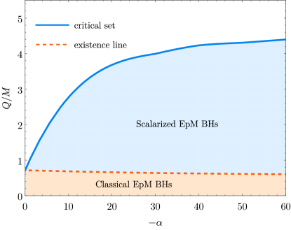
Figure 1: Part of the domain of existence of spherical scalarized EPM BHs with $n=3/5$ in the $(\alpha,q)$–plane.

Note that there exists a region of non-uniqueness within the domain of existence where scalar–free and scalarized BHs coexist, as defined by the values of $q$ for which the metric $N$ possesses real roots. In this region, the scalarized solution is entropically preferred, as they maximize the entropy (or, equivalently, the horizon area $A_{H}$), as shown in Figure 2 for the specific values indicated in the legend. It is worth highlighting that, for varying values of $\alpha$, the $a_{H}$-curves (as defined in the caption of Figure 2) exhibit no significant deviation from one another.

Figure 2: $a_{H}=A_{H}/(16\pi M^{2})$ vs. $q=Q/M$ diagram, where $A_{H}$ is the horizon area of scalarized (solid line) and scalar–free (dashed line) EpM BHs with $\alpha=-100$.

An illustrative solution is shown in Figure 3 and Figure 4 for $Q=0.3$, $\alpha=-50$ and specific values of $r_{H}$ indicated in the legend. Note that the behavior of the whole functions coincides with the scalarized RN BH in Herdeiro:2018wub .

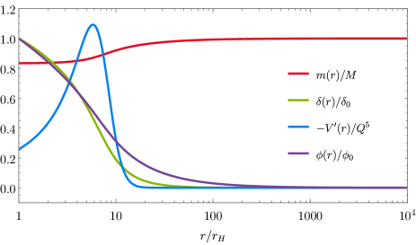
Figure 3: Metric and matter functions of a scalarized EpM BH with $Q=0.3$, $\alpha=-50$ and $r_{H}=0.1$.

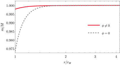
Figure 4: Mass function of a scalarized EpM and a scalar-free EpM BHs, with $Q=0.3$, $\alpha=-50$, $r_{H}^{\phi\neq 0}=0.95$ and $r_{H}^{\phi=0}=0.9177$.

V Conclusions

In this work, we analyzed the spontaneous scalarization undergone by an Einstein-power-Maxwell system non–minimally coupled to a scalar field. We obtained that, based on the virial identity, the power of the Maxwell scalar $F_{\mu\nu}F^{\mu\nu}$ cannot take any arbitrary value, but it must be constrained in a very specific way to ensure scalarization. We focused on the case $n<1$ and set the power in a way that the free solution corresponds to a straightforward modification of the RN metric, namely, a metric containing a term proportional to $r^{-\beta}$, with $\beta\in\mathbb{N}$. The motivation behind this choice was that considering $\beta$ as an integer is the most “natural” way to modify the mass function of the Schwarzschild BH, namely $m(r)=M-\xi/r^{\beta-1}$ ($\xi$ being a constant). For example, if $\beta=2$, the RN solution is recovered. If $\beta$ is arbitrary, the metric falls into the family of Kiselev solutions Kiselev:2002dx . Framed in a power-Maxwell model, this modification of the mass function leads to certain values of $n$ that would not be as natural to choose if we did not have the guidance of the mass function (like $n=3/5$, in our case). Furthermore, our model shows advantages in comparison with the RN case because the domain of existence is significantly distinct from the $n=1$ scenario. Notably, the entire ($\alpha,q$)-range is expanded and the domain of the classical EpM BHs is extended, underscoring a clear advantage over the proposal outlined in  Herdeiro:2018wub . Moreover, our findings demonstrated that the scalarized solutions are entropically favored in comparison to their hairless counterpart, in agreement with what occurs for the scalarized RN BHs in Herdeiro:2018wub . It could be interesting to explore arbitrary $(n,l,m)$ scalar clouds and to study the stability of the solution against perturbations. However, these and other aspects lie out of the scope of the present work and we leave them for future developments.

VI Acknowledgements

M.C expresses sincere gratitude to C. A. R. Herdeiro and the Gr@v Group at the University of Aveiro for their warm hospitality during the development of this work. This work is supported by the Center for Research and Development in Mathematics and Applications (CIDMA) through the Portuguese Foundation for Science and Technology (FCT – Fundação para a Ciência e a Tecnologia), references UIDB/04106/2020 and UIDP/04106/2020. The authors acknowledge support from the projects PTDC/FIS-AST/3041/2020 and CERN/FIS-PAR/0024/2021. This work has further been supported by the European Horizon Europe staff exchange (SE) programme HORIZON-MSCA-2021-SE-01 Grant No. NewFunFiCO-101086251. M.C acknowledges to the Master in Physics program at USFQ for financial support. N. M. S. is supported by the FCT grant SFRH/BD/143407/2019.

References

- [1] B. P. Abbott et al. Observation of Gravitational Waves from a Binary Black Hole Merger. Phys. Rev. Lett., 116(6):061102, 2016.
- [2] Kazunori Akiyama et al. First M87 Event Horizon Telescope Results. I. The Shadow of the Supermassive Black Hole. Astrophys. J. Lett., 875:L1, 2019.
- [3] Carlos A. R. Herdeiro and Eugen Radu. Asymptotically flat black holes with scalar hair: a review. Int. J. Mod. Phys. D, 24(09):1542014, 2015.
- [4] Remo Ruffini and John A. Wheeler. Introducing the black hole. Phys. Today, 24(1):30, 1971.
- [5] Daniela D. Doneva and Stoytcho S. Yazadjiev. New Gauss-Bonnet Black Holes with Curvature-Induced Scalarization in Extended Scalar-Tensor Theories. Phys. Rev. Lett., 120(13):131103, 2018.
- [6] Hector O. Silva, Jeremy Sakstein, Leonardo Gualtieri, Thomas P. Sotiriou, and Emanuele Berti. Spontaneous scalarization of black holes and compact stars from a Gauss-Bonnet coupling. Phys. Rev. Lett., 120(13):131104, 2018.
- [7] G. Antoniou, A. Bakopoulos, and P. Kanti. Evasion of No-Hair Theorems and Novel Black-Hole Solutions in Gauss-Bonnet Theories. Phys. Rev. Lett., 120(13):131102, 2018.
- [8] Thibault Damour and Gilles Esposito-Farese. Nonperturbative strong field effects in tensor - scalar theories of gravitation. Phys. Rev. Lett., 70:2220–2223, 1993.
- [9] Masato Minamitsuji and Taishi Ikeda. Scalarized black holes in the presence of the coupling to Gauss-Bonnet gravity. Phys. Rev. D, 99(4):044017, 2019.
- [10] Jose Luis Blázquez-Salcedo, Daniela D. Doneva, Jutta Kunz, and Stoytcho S. Yazadjiev. Radial perturbations of the scalarized Einstein-Gauss-Bonnet black holes. Phys. Rev. D, 98(8):084011, 2018.
- [11] Hector O. Silva, Caio F. B. Macedo, Thomas P. Sotiriou, Leonardo Gualtieri, Jeremy Sakstein, and Emanuele Berti. Stability of scalarized black hole solutions in scalar-Gauss-Bonnet gravity. Phys. Rev. D, 99(6):064011, 2019.
- [12] William E. East and Justin L. Ripley. Dynamics of Spontaneous Black Hole Scalarization and Mergers in Einstein-Scalar-Gauss-Bonnet Gravity. Phys. Rev. Lett., 127(10):101102, 2021.
- [13] Pedro V. P. Cunha, Carlos A. R. Herdeiro, and Eugen Radu. Spontaneously Scalarized Kerr Black Holes in Extended Scalar-Tensor–Gauss-Bonnet Gravity. Phys. Rev. Lett., 123(1):011101, 2019.
- [14] Carlos A. R. Herdeiro, Eugen Radu, Hector O. Silva, Thomas P. Sotiriou, and Nicolás Yunes. Spin-induced scalarized black holes. Phys. Rev. Lett., 126(1):011103, 2021.
- [15] Caio F. B. Macedo, Jeremy Sakstein, Emanuele Berti, Leonardo Gualtieri, Hector O. Silva, and Thomas P. Sotiriou. Self-interactions and Spontaneous Black Hole Scalarization. Phys. Rev. D, 99(10):104041, 2019.
- [16] Alexandru Dima, Enrico Barausse, Nicola Franchini, and Thomas P. Sotiriou. Spin-induced black hole spontaneous scalarization. Phys. Rev. Lett., 125(23):231101, 2020.
- [17] Fahimeh Rahimi and Zeinab Rezaei. Spontaneous scalarization in proto-neutron stars. Eur. Phys. J. C, 83(4):289, 2023.
- [18] Takami Kuroda and Masaru Shibata. Spontaneous scalarization as a new core-collapse supernova mechanism and its multimessenger signals. Phys. Rev. D, 107(10):103025, 2023.
- [19] Sebastian Bahamonde, Daniela D. Doneva, Ludovic Ducobu, Christian Pfeifer, and Stoytcho S. Yazadjiev. Spontaneous scalarization of black holes in Gauss-Bonnet teleparallel gravity. Phys. Rev. D, 107(10):104013, 2023.
- [20] Kalin V. Staykov and Daniela D. Doneva. Multiscalar Gauss-Bonnet gravity: Scalarized black holes beyond spontaneous scalarization. Phys. Rev. D, 106(10):104064, 2022.
- [21] Daniela D. Doneva, Lucas G. Collodel, and Stoytcho S. Yazadjiev. Spontaneous nonlinear scalarization of Kerr black holes. Phys. Rev. D, 106(10):104027, 2022.
- [22] Peng Wang, Houwen Wu, and Haitang Yang. Scalarized Einstein-Born-Infeld black holes. Phys. Rev. D, 103(10):104012, 2021.
- [23] Daniela D. Doneva, Fethi M. Ramazanoğlu, Hector O. Silva, Thomas P. Sotiriou, and Stoytcho S. Yazadjiev. Scalarization. 11 2022.
- [24] Carlos A. R. Herdeiro, Eugen Radu, Nicolas Sanchis-Gual, and José A. Font. Spontaneous Scalarization of Charged Black Holes. Phys. Rev. Lett., 121(10):101102, 2018.
- [25] Yun Soo Myung and De-Cheng Zou. Instability of Reissner–Nordström black hole in Einstein-Maxwell-scalar theory. Eur. Phys. J. C, 79(3):273, 2019.
- [26] Yun Soo Myung and De-Cheng Zou. Quasinormal modes of scalarized black holes in the Einstein–Maxwell–Scalar theory. Phys. Lett. B, 790:400–407, 2019.
- [27] Carlos A. R. Herdeiro and Eugen Radu. Black hole scalarization from the breakdown of scale invariance. Phys. Rev. D, 99(8):084039, 2019.
- [28] Pedro G. S. Fernandes, Carlos A. R. Herdeiro, Alexandre M. Pombo, Eugen Radu, and Nicolas Sanchis-Gual. Spontaneous Scalarisation of Charged Black Holes: Coupling Dependence and Dynamical Features. Class. Quant. Grav., 36(13):134002, 2019. [Erratum: Class.Quant.Grav. 37, 049501 (2020)].
- [29] Yves Brihaye and Betti Hartmann. Spontaneous scalarization of charged black holes at the approach to extremality. Phys. Lett. B, 792:244–250, 2019.
- [30] Carlos A. R. Herdeiro and João M. S. Oliveira. On the inexistence of solitons in Einstein–Maxwell-scalar models. Class. Quant. Grav., 36(10):105015, 2019.
- [31] Yun Soo Myung and De-Cheng Zou. Stability of scalarized charged black holes in the Einstein–Maxwell–Scalar theory. Eur. Phys. J. C, 79(8):641, 2019.
- [32] D. Astefanesei, C. Herdeiro, A. Pombo, and E. Radu. Einstein-Maxwell-scalar black holes: classes of solutions, dyons and extremality. JHEP, 10:078, 2019.
- [33] R. A. Konoplya and A. Zhidenko. Analytical representation for metrics of scalarized Einstein-Maxwell black holes and their shadows. Phys. Rev. D, 100(4):044015, 2019.
- [34] Roman A. Konoplya, Thomas Pappas, and Alexander Zhidenko. Einstein-scalar–Gauss-Bonnet black holes: Analytical approximation for the metric and applications to calculations of shadows. Phys. Rev. D, 101(4):044054, 2020.
- [35] Pedro G. S. Fernandes, Carlos A. R. Herdeiro, Alexandre M. Pombo, Eugen Radu, and Nicolas Sanchis-Gual. Charged black holes with axionic-type couplings: Classes of solutions and dynamical scalarization. Phys. Rev. D, 100(8):084045, 2019.
- [36] De-Cheng Zou and Yun Soo Myung. Scalarized charged black holes with scalar mass term. Phys. Rev. D, 100(12):124055, 2019.
- [37] Carlos A. R. Herdeiro, João M. S. Oliveira, and Eugen Radu. A class of solitons in Maxwell-scalar and Einstein–Maxwell-scalar models. Eur. Phys. J. C, 80(1):23, 2020.
- [38] Shahar Hod. Spontaneous scalarization of charged Reissner-Nordström black holes: Analytic treatment along the existence line. Phys. Lett. B, 798:135025, 2019.
- [39] Jose Luis Blázquez-Salcedo, Carlos A. R. Herdeiro, Jutta Kunz, Alexandre M. Pombo, and Eugen Radu. Einstein-Maxwell-scalar black holes: the hot, the cold and the bald. Phys. Lett. B, 806:135493, 2020.
- [40] Pedro G. S. Fernandes. Einstein–Maxwell-scalar black holes with massive and self-interacting scalar hair. Phys. Dark Univ., 30:100716, 2020.
- [41] Carlos A. R. Herdeiro and João M. S. Oliveira. Electromagnetic dual Einstein-Maxwell-scalar models. JHEP, 07:130, 2020.
- [42] Shahar Hod. Reissner-Nordström black holes supporting nonminimally coupled massive scalar field configurations. Phys. Rev. D, 101(10):104025, 2020.
- [43] Shuang Yu, Jianhui Qiu, and Changjun Gao. Constructing black holes in Einstein–Maxwell-scalar theory. Class. Quant. Grav., 38(10):105006, 2021.
- [44] Jose Luis Blázquez-Salcedo, Carlos A. R. Herdeiro, Sarah Kahlen, Jutta Kunz, Alexandre M. Pombo, and Eugen Radu. Quasinormal modes of hot, cold and bald Einstein–Maxwell-scalar black holes. Eur. Phys. J. C, 81(2):155, 2021.
- [45] Yun Soo Myung and De-Cheng Zou. Scalarized charged black holes in the Einstein-Maxwell-Scalar theory with two U(1) fields. Phys. Lett. B, 811:135905, 2020.
- [46] Carlos A. R. Herdeiro, Taishi Ikeda, Masato Minamitsuji, Tomohiro Nakamura, and Eugen Radu. Spontaneous scalarization of a conducting sphere in Maxwell-scalar models. Phys. Rev. D, 103(4):044019, 2021.
- [47] Jose Luis Blázquez-Salcedo, Sarah Kahlen, and Jutta Kunz. Critical solutions of scalarized black holes. Symmetry, 12(12):2057, 2020.
- [48] Yun Soo Myung and De-Cheng Zou. Scalarized black holes in the Einstein-Maxwell-scalar theory with a quasitopological term. Phys. Rev. D, 103(2):024010, 2021.
- [49] Shahar Hod. Analytic treatment of near-extremal charged black holes supporting non-minimally coupled massless scalar clouds. Eur. Phys. J. C, 80(12):1150, 2020.
- [50] Guangzhou Guo, Peng Wang, Houwen Wu, and Haitang Yang. Scalarized Einstein–Maxwell-scalar black holes in anti-de Sitter spacetime. Eur. Phys. J. C, 81(10):864, 2021.
- [51] Feiyu Yao. Scalarized Einstein–Maxwell-scalar black holes in a cavity. Eur. Phys. J. C, 81(11):1009, 2021.
- [52] Cheng-Yong Zhang, Qian Chen, Yunqi Liu, Wen-Kun Luo, Yu Tian, and Bin Wang. Critical Phenomena in Dynamical Scalarization of Charged Black Holes. Phys. Rev. Lett., 128(16):161105, 2022.
- [53] Wei Xiong, Peng Liu, Chao Niu, Cheng-Yong Zhang, and Bin Wang. Dynamical spontaneous scalarization in Einstein-Maxwell-scalar theory *. Chin. Phys. C, 46(9):095103, 2022.
- [54] Shahar Hod. Spin-charge induced scalarization of Kerr-Newman black-hole spacetimes. JHEP, 08:272, 2022.
- [55] Chao Niu, Wei Xiong, Peng Liu, Cheng-Yong Zhang, and Bin Wang. Dynamical descalarization in Einstein-Maxwell-scalar theory. 9 2022.
- [56] Jie Jiang and Jia Tan. Spontaneous scalarization of dyonic black hole in Einstein–Maxwell-scalar theory. Eur. Phys. J. C, 83(4):290, 2023.
- [57] Jia-Yan Jiang, Qian Chen, Yunqi Liu, Yu Tian, Wei Xiong, Cheng-Yong Zhang, and Bin Wang. Type I critical dynamical scalarization and descalarization in Einstein-Maxwell-scalar theory. 6 2023.
- [58] Guangzhou Guo, Peng Wang, Houwen Wu, and Haitang Yang. Scalarized Kerr-Newman Black Holes. 7 2023.
- [59] Shahar Hod. Analytic study of the Maxwell electromagnetic invariant in spinning and charged Kerr-Newman black-hole spacetimes. JHEP, 09:140, 2023.
- [60] Stella Kiorpelidi, Thanasis Karakasis, George Koutsoumbas, and Eleftherios Papantonopoulos. Scalarization of the Reissner-Nordsröm black hole with higher gauge field corrections. 11 2023.
- [61] Zakaria Belkhadria and Alexandre M. Pombo. Mixed scalarization of charged black holes: from spontaneous to non-linear scalarization. 11 2023.
- [62] M. Born. Modified field equations with a finite radius of the electron. Nature, 132(3329):282.1, 1933.
- [63] Eloy Ayon-Beato and Alberto Garcia. Regular black hole in general relativity coupled to nonlinear electrodynamics. Phys. Rev. Lett., 80:5056–5059, 1998.
- [64] Eloy Ayon-Beato and Alberto Garcia. New regular black hole solution from nonlinear electrodynamics. Phys. Lett. B, 464:25, 1999.
- [65] Kirill A. Bronnikov. Regular magnetic black holes and monopoles from nonlinear electrodynamics. Phys. Rev. D, 63:044005, 2001.
- [66] Leonardo Balart and Elias C. Vagenas. Regular black holes with a nonlinear electrodynamics source. Phys. Rev. D, 90(12):124045, 2014.
- [67] Irina Dymnikova and Evgeny Galaktionov. Regular rotating electrically charged black holes and solitons in non-linear electrodynamics minimally coupled to gravity. Class. Quant. Grav., 32(16):165015, 2015.
- [68] Manuel E. Rodrigues, Ednaldo L. B. Junior, and Marcos V. de Sousa Silva. Using dominant and weak energy conditions for build new classe of regular black holes. JCAP, 02:059, 2018.
- [69] K. A. Bronnikov. Nonlinear electrodynamics, regular black holes and wormholes. Int. J. Mod. Phys. D, 27(06):1841005, 2018.
- [70] Mokhtar Hassaine and Cristian Martinez. Higher-dimensional black holes with a conformally invariant Maxwell source. Phys. Rev. D, 75:027502, 2007.
- [71] Mokhtar Hassaine and Cristian Martinez. Higher-dimensional charged black holes solutions with a nonlinear electrodynamics source. Class. Quant. Grav., 25:195023, 2008.
- [72] Ángel Rincón, Ernesto Contreras, Pedro Bargueño, Benjamin Koch, and Grigoris Panotopoulos. Four dimensional Einstein-power-Maxwell black hole solutions in scale-dependent gravity. Phys. Dark Univ., 31:100783, 2021.
- [73] V. V. Kiselev. Quintessence and black holes. Class. Quant. Grav., 20:1187–1198, 2003.