Three-flavor Collective Neutrino Oscillations on D-Wave’s Advantage Quantum Annealer

Abstract

In extreme environments such as core-collapse supernovae, neutron-star mergers, and the early Universe, neutrinos are dense enough that their self-interactions significantly affect, if not dominate, their flavor dynamics. In order to develop techniques for characterizing the resulting quantum entanglement, I present the results of simulations of Dirac neutrino-neutrino interactions that include all three physical neutrino flavors and were performed on D-Wave Inc.’s Advantage 5000+ qubit quantum annealer. These results are checked against those from exact classical simulations, which are also used to compare the Dirac neutrino-neutrino interactions to neutrino-antineutrino and Majorana neutrino-neutrino interactions. The D-Wave Advantage annealer is shown to be able to reproduce time evolution with the precision of a classical machine for small numbers of neutrinos and to do so without Trotter errors. However, it suffers from poor scaling in qubit-count with the number of neutrinos. Two approaches to improving the qubit-scaling are discussed, but only one of the two shows promise.

I Introduction

In extreme-density and extreme-temperature environments, such as core-collapse supernovae (CCSNe), neutron-star mergers and the early Universe, neutrinos dominate the transport of energy, momentum, entropy, neutron-to-proton ratios, and lepton flavor composition, among other characteristics (for recent reviews, see Refs. [1, 2, 3, 4, 5]). Several neutron star merger studies show neutrinos having an effect in phenomena such as mass ejection and accretion, as well as gamma-ray burst formation [6, 7, 8]. In CCSNe, neutrinos carry away 99% of the gravitational binding energy released by the collapse of the iron core at the supernova’s beginning [9, 10, 11, 12, 13, 14, 15, 16, 17, 18, 19]. There is also a consensus in the field that these neutrinos are the primary triggering mechanism in most CCSNe [20, 21, 9, 22, 23, 24, 25, 26]. Neutrinos are also thought to play a key role in nucleosynthesis in all three of the above phenomena, with a few light isotopes and several heavy ones being particularly dependent on neutrino processes [27, 28, 29, 30, 31, 32, 33, 29].

One challenge is that at such high densities and temperatures, neutrino-neutrino interactions, which manifest as collective neutrino oscillations, are significant enough to produce macroscopic effects. Recent simulations have shown that a few neutrino-dependent processes which are theorized to be critical in the nucleosynthesis of nuclei with mass numbers above 64 are heavily dependent on collective neutrino oscillations [28, 34, 35]. Collective neutrino oscillations are also expected to have an effect on r-process, which is responsible for half of the abundance of elements in the Universe heavier than iron [36]. In short, collective neutrino oscillations must be taken into account in order to fully understand the dynamics of neutrinos in high-temperature, high-density astrophysical phenomena.

Collective neutrino oscillations are a highly nonlinear many-body problem [37, 38, 39]. One commonly-used method for many-body problems like this one is mean-field theory, which treats all but the observed neutrino as a single-valued background interacting with said neutrino [40]. This approach is effective in achieving a linear scaling of computational resources with system size. However, it is unable to simulate quantum entanglement and incoherent scattering. Whether this fact invalidates the use of mean-field theory in macroscopic neutrino systems is still an unanswered question [41].

Meanwhile, methods that do account for entanglement in collective neutrino oscillations have been utilized extensively. They include exact time evolution through numerical integration or diagonalization of the equations of motion, the Bethe ansatz, and tensor network algorithms [42, 43, 44, 45, 46, 47, 48, 49, 50, 51, 52, 53, 54, 55, 56, 57, 58, 59]. For neutrino systems so dense that neutrino-neutrino interaction is the only term that needs to be considered, generalized angular momentum representations can be used to simulate up to O($10^{6}$) neutrinos [60, 61, 62, 63, 64]. However, as is the case with many simulations of quantum-mechanical phenomena, the resources needed to study entanglement in collective neutrino oscillations on classical computers scale exponentially with the size of the system in the general case [65, 66, 35, 67, 54, 68]. As a result, simulations of collective neutrino oscillations in the using exact numerical methods have been limited to up to 20 neutrinos. Tensor network [53, 54, 55] and matrix product state methods [43, 69, 70], which are two of the leading methods of approximate simulation of quantum mechanical systems, can simulate considerably more neutrinos. For instance, the time-dependent variational principle (TDVP) can currently be used to simulate up to approximately 50 neutrinos if the neutrinos start in the same flavor, though simulable system size is likely to be smaller for a mix of initial flavors [55]. However, the fundamental problem of exponential scaling of computational resource requirements with system size still has not been solved. This presents an opportunity for quantum computers to produce an advantage, as they are capable of efficiently simulating any local quantum system [71, 72]. Simulations of two-flavor collective neutrino oscillations have been done on devices such as Quantinuum’s trapped ion devices [73, 74], IBM’s superconducting devices [66, 75, 76], and D-Wave’s Advantage quantum annealer [77]. For a recent review of the entire field of collective neutrino oscillations, see Ref. [67].

The above studies have only simulated neutrinos under the assumption that the number of possible neutrino flavors, $n_{f}$, is 2, with the physical $n_{f}$ = 3 collective neutrino oscillation picture being analyzed entirely in mean-field theory [78, 79, 80, 81, 82, 83, 34, 84, 85, 86] until last year, when the first exact calculations of three-flavor collective neutrino oscillations were done [68, 65]. Ref. [68] found a difference between results for $n_{f}$ = 3 and those for $n_{f}$ = 2. One of the limitations of the first two exact $n_{f}$ = 3 studies was that they used the single-angle approximation. Physically, neutrino-neutrino interactions depend on the angle between the trajectories of the interacting neutrinos. However, in the single-angle approximation, the trajectory-directions are averaged over [87]. Supernova models that use the single-angle approximation exhibit several differences with those that do not [88, 89, 90, 91, 92]. For instance, the single-angle approximation produces collective neutrino oscillations at earlier times than the full (“multi-angle”) treatment of each neutrino’s trajectory [93]. These differences reflect themselves in supernova neutrino spectra [34, 94, 95, 96, 81, 97, 95] and in nucleosynthesis [36].

Thus, it is important to the astrophysical applications of neutrino science to devise techniques for multi-angle simulations of collective neutrino oscillations with $n_{f}$ = 3, and to create algorithms by which future quantum computers can efficiently compute such simulations. This paper details the extension of the two-flavor collective neutrino oscillation analysis in Ref. [77] to three flavors. This is the first attempt to implement collective neutrino oscillations with number of flavors $n_{f}$ = 3 on a quantum device, and the first to do so in a multi-angle formalism.

This paper is organized as follows. In Section II, the Hamiltonian that defines the dynamics of the collective neutrino oscillations is established and discussed. In Section III, the techniques for implementing dynamics on D-Wave’s Advantage quantum annealer are described. Section IV presents the results of the simulation. Section V covers attempts to obtain scaling quantum advantage on a quantum annealer. Section VI discusses extension of the study to antineutrinos, Majorana neutrinos, and to time-dependent neutrino-neutrino interactions. Section VII discusses the implications of the results and future directions of research. Appendices discuss technical details.

II Collective Neutrino Oscillation Hamiltonian

The terms relevant to the construction of a Hamiltonian describing collective neutrino oscillations are the vacuum propagation (which effects neutrino oscillations), the neutrino-neutrino interactions [37, 38, 39], and the matter-neutrino interactions (MSW effects) [98, 99, 100]. Like in Refs. [68, 52, 55, 101, 44, 102, 47, 103, 50, 51] the neutrino vacuum propagation and neutrino-neutrino interaction terms are assumed to be dominant over the MSW effects. The neutrino-neutrino terms are dependent on neutrino density [104] and hence are time-dependent in physical applications, as neutrinos radiate outward from a source and their density decreases as they do so. However, one of the primary aims of this study is to devise techniques for simulation on the Advantage quantum annealer. For this reason, the Hamiltonian is treated as time-independent, following the lead of Ref. [77]. Additionally, only interactions that either preserve or exchange the neutrino momenta (“forward scattering”) are taken into account. Discussion in the literature of non-forward scattering has been taking place for decades [105, 106, 60, 107, 108, 109, 110, 104, 44, 47, 49, 54, 53, 64, 62, 63, 101, 55, 57, 111]. While the first quantum many-body study of collective neutrino oscillations that included the full forward and non-forward scattering was recently done [58], in this work the forward scattering approximation is used, in the interest of a simple mapping of the problem onto quantum devices.

$n_{f}$ = 3 collective neutrino oscillations of N neutrinos in the mass basis can be represented in terms of the Gell-Mann matrices [104, 68]:

$$H_{CNO}=\sum_{p=1}^{N}\vec{B}\cdot\vec{\lambda}_{p}+\sum_{p=1}^{N-1}\sum_{p^{\prime}=p+1}^{N}k(1-\cos{\theta_{pp^{\prime}}})\vec{\lambda}_{p}\cdot\vec{\lambda}_{p^{{}^{\prime}}}$$ (1)

where $\vec{\lambda}_{p}$ is the 8-term vector composed of the Gell-Mann matrices applied to the neutrino indexed by $p$, $\theta_{pp^{\prime}}$ is the angle between the momenta of the neutrinos indexed by $p$ and $p^{\prime}$, $k$ is the coupling strength of the neutrino-neutrino interaction, E is the energy of the neutrino in question, and $\vec{B}$ is a vector that creates the diagonalized single-neutrino oscillation term when dotted with $\vec{\lambda}_{p}$. The diagonalized single-vector neutrino oscillation term is determined by two parameters: $\delta m^{2}$, the difference in mass-squared between the first and second mass eigenstates, and $\Delta m^{2}$, the difference between the third mass eigenstate’s mass-squared and the mean of the masses-squared of the first and second mass eigenstates (following the convention of Ref. [112]). It turns out that two neutrinos with the same starting state and with the same momentum behave exactly the same as if they were just one neutrino. Hence, following the lead of Ref. [68], a neutrino referenced by p can be thought of as a momentum-mode. In order to convert between the flavor and mass basis, the PMNS matrix [113, 114, 115] is utilized:

$$U_{PMNS}=\begin{pmatrix}1&0&0\\ 0&c_{23}&s_{23}\\ 0&-s_{23}&{}_{23}\\ \end{pmatrix}\begin{pmatrix}c_{13}&0&s_{13}e^{-i\delta}\\ 0&1&0\\ -s_{13}e^{i\delta}&0&c_{13}\\ \end{pmatrix}\begin{pmatrix}c_{12}&s_{12}&0\\ -s_{12}&c_{12}&0\\ 0&0&1\\ \end{pmatrix}$$ (2)

where $c_{ij}=\cos{\theta_{ij}}$ and $s_{ij}=\sin{\theta_{ij}}$. One feature of Eq. 1 is that as long as the absolute values of the neutrino energies are all the same, the single-neutrino term commutes with the neutrino-neutrino interaction term. Related to this, the neutrino-neutrino interaction term is independent of the basis that the neutrinos are in, so long as the neutrinos are all in the same basis. This fact enables the strategy utilized in Sec. IV to work and has several consequences for the observations therein.

The parameters used in this project can be found in Tab. 1. The single-neutrino term parameters are drawn from Ref. [68] and fall within the 1 $\sigma$ confidence interval of experimental results if rounded to three significant figures as of the release of the 2023 PDG Review [116]. For N = 4, the angles $\theta_{ij}$ between the neutrinos, used for the neutrino-neutrino interaction term, are given by the anisotropic angle distribution from Ref. [77], with $\xi$ = 0.9:

$$\theta_{ij}=\arccos{(\xi)}\frac{\absolutevalue{i-j}}{N-1}$$ (3)

Parameter	Values	PDG Experimental results
$E_{i}$	$10^{7}$ eV	n/a
$\delta m^{2}$	$7.42*10^{-5}$ eV	$(7.53(18))*10^{-5}$ eV
$\Delta m^{2}$	$2.44*10^{-3}$ eV	$(2.475(33))*10^{-3}$ eV
${\theta_{v}}_{12}$	0.591667	$0.587(14)$
${\theta_{v}}_{13}$	0.148702	$0.1489(24)$
${\theta_{v}}_{23}$	0.840027	$0.832(^{+18}_{-12})$
$\delta$	4.36681	$3.86(66)$
$\theta_{12}$ (N = 2)	$\frac{\pi}{4}$	n/a
$\theta_{ij}$ (N = 4)	Eq. 3	n/a
$k$	$1.75*10^{-12}$	n/a

Table 1: The parameters used in the exact simulation of $n_{f}$ = 3 interacting neutrino systems described by Eq. 1 as well as the experimental results from the 2023 PDG Review [116] for neutrino oscillation terms. For all $n_{f}$ = 2 studies, unless otherwise stated, the mass-difference is set to $\Delta m^{2}$ and the mixing angle to ${\theta_{v}}_{12}$

.

III Implementation on D-Wave Advantage Quantum Annealer

D-Wave’s Advantage quantum annealer is a 5000+-qubit device [117] designed with the express function of obtaining the ground state of a user-specified classical Ising model through a procedure known as quantum annealing. In quantum annealing, the system begins in the ground state of one Hamiltonian $H_{i}$ and is time-evolved on a Hamiltonian $H_{a}$ that begins as $H_{i}$ but gradually becomes a different Hamiltonian, $H_{f}$. As long as $H_{a}$’s transition from $H_{i}$ to $H_{f}$ is sufficiently slow, the system’s final state will be the ground state of $H_{f}$ [118]. For Advantage, $H_{i}=(\sum_{i}\hat{\sigma}^{(i)}_{x})$ and $H_{f}=(\sum_{i}h_{i}\hat{\sigma}^{(i)}_{z}+\sum_{i>j}J_{ij}\hat{\sigma}^{(i)}_{z}\hat{\sigma}^{(j)}_{z})$, where $\hat{\sigma}^{(i)}_{x}$ and $\hat{\sigma}^{(i)}_{z}$ are the Pauli-x and Pauli-z matrices, respectively, acting on the $i^{th}$ qubit, and $h_{i}$ and $J_{ij}$ are the user-tunable parameters. In turn, $H_{a}$ is set to the following Hamiltonian [119]:

$$H_{ising}=\frac{A(s)}{2}(\sum_{i}\hat{\sigma}^{(i)}_{x})+\frac{B(s)}{2}(\sum_{i}h_{i}\hat{\sigma}^{(i)}_{z}+\sum_{i>j}J_{ij}\hat{\sigma}^{(i)}_{z}\hat{\sigma}^{(j)}_{z})$$ (4)

where A(s) and B(s) are time-dependent parameters. s is a time-parameter, defined as $s=t/t_{f}$, where t is time and $t_{f}$ is the total time of the anneal. In order for quantum annealing to be executed, A(s) and B(s) are defined so that $A(0)>>B(0)$ and $A(1)<<B(1)$. The exact definitions of A(s) and B(s) are known as the annealing schedule.

One of the main documentation-prescribed methods of mapping an optimization problem onto Advantage is to map it onto a QUBO (quadratic unconstrained binary optimization) problem [120, 119, 117]. A QUBO problem is one that involves the minimization of a function of the form

$$f(x)=\sum_{i}Q_{ii}\bf{x}_{i}+\sum_{i<j}Q_{ij}\bf{x}_{i}\bf{x}_{j}$$ (5)

with $\bf{x}_{i}$ being a binary variable with 2 possible values: 0 or 1.

QUBO problems are directly mappable onto Advantage’s $H_{f}$ [117] and one can directly submit a problem with a given set of $Q_{ij}$ values to the Ocean interface provided by DWave Systems, which will convert it to a set of $h_{i}$ and $J_{ij}$ parameters to be submitted directly to the annealer [119].

Advantage’s hardware runs on an architecture known as Chimaera. This means that the two-qubit couplings $J_{ij}$ can act between any qubit and one of the 15 other qubits on Advantage that Chimaera connects it to [117]. However, collective neutrino oscillations require coupling between all pairs of simulated neutrinos. The required all-to-all coupling is obtained on Advantage through a process called minor-embedding. Minor-embedding works by mapping each logical qubit to a set of physical qubits called a “chain”. All qubits in a chain are fixed to the same value by setting the $Q_{ij}$ parameters between them to a negative value high enough in magnitude (which is called the “chain-strength”) to do so and that is set by the user [119]. In this project, the chain-strength is set to 1, because it is high enough to prevent almost all differences in value between qubits in a chain (“chain-breaks”), and higher values have been found to interfere with convergence to the final ground state. Because all of the qubits in a chain are the same value, the chains can be treated as 1 qubit with a connectivity equal to the sum of the connectivities of the qubits minus the number of connections between qubits on the same chain. In this project, D-Wave’s provided minor-embedders, which have a quadratic complexity [119], are used for this purpose.

III.1 Mapping time evolution onto a QUBO problem

Time-evolution is encoded in an annealer through a Feynman clock Hamiltonian [121]:

$$C=C_{0}+\frac{1}{2}\sum_{t}(I\otimes\ket{t}\bra{t}-U_{t}\otimes\ket{t+dt}\bra{t}-U_{t}^{\dagger}\otimes\ket{t+dt}\bra{t}+I\otimes\ket{t+dt}\bra{t+dt})$$ (6)

The point of the Feynman clock Hamiltonian is to have a separate qubit-register for the system for each sampled time, and for the ground state of the Feynman clock Hamiltonian to equal the state of the system at each sampled time. Here, $C_{0}=(I-\ket{\Psi_{0}}\bra{\Psi_{0}})\otimes\ket{0}\bra{0}$ is a penalty term that ensures that the desired initial state $\ket{\Psi_{0}}$ is the ground state of the initial time register and $U_{t}=e^{-iHdt}$ is the time-evolution operator for Hamiltonian H across a time-increment dt.

The matrix form of the Feynman clock Hamiltonian is digitized (with a register of K qubits representing each state-amplitude) in order to map it to a QUBO problem. The digitization, following the lead of Refs [122, 77], works as follows:

$$a_{\alpha}=-2q_{K}^{\alpha}+\sum_{i=1}^{K-1}\frac{q_{i}^{\alpha}}{2^{K-i}}$$ (7)

with $a_{\alpha}$ being the $\alpha^{th}$ element of the original state-vector $a$ and the $q^{\alpha}_{i}$ is the $i^{th}$ digit in the digitization of $a_{\alpha}$. Each $q^{\alpha}_{i}$ can be either 0 or 1 when measured. K is a digitization parameter that denotes the precision at which to truncate the digitization. If one works in a basis where the Hamiltonian submitted to the annealer is real, then one can simply apply the digitization to the said Hamiltonian and it would be ready to submit to the annealer. However, the Feynman clock Hamiltonian by default is complex, and so must be mapped to a real matrix so that it is submittable as a QUBO model. This is done using the method used in Refs. [123, 77]. The size of the statevector-space is doubled, and half of the result is delegated to the real component and the other half to the imaginary component. The resulting breakdown of the Feynman clock Hamiltonian is as follows:

$$\bar{a}_{\alpha}a_{\beta}C_{\alpha\beta}=\bar{a}_{\alpha}^{Re}a_{\beta}^{Re}C_{\alpha\beta}^{Re}-\bar{a}_{\alpha}^{Re}a_{\beta}^{Im}C^{Im}_{\alpha\beta}+\bar{a}_{\alpha}^{Im}a_{\beta}^{Re}C^{Im}_{\alpha\beta}+\bar{a}_{\alpha}^{Im}a_{\beta}^{Im}C^{Re}_{\alpha\beta}$$ (8)

Combining Eq. 7 and 8 leads us to

$$Q_{\alpha,i;\beta,j}=\begin{cases}2^{i+j-2K}(-1)^{\delta_{iK}+\delta_{jK}}C^{Re}_{\alpha\beta},&\text{if }1\leq i,j\leq K,\\ -2^{i+j^{\prime}-2K}(-1)^{\delta_{iK}+\delta_{j^{\prime}K}}C^{Im}_{\alpha\beta},&\text{if }1\leq i,j^{\prime}\leq K,\\ 2^{i^{\prime}+j-2K}(-1)^{\delta_{i^{\prime}K}+\delta_{jK}}C^{Im}_{\alpha\beta},&\text{if }1\leq i^{\prime},j\leq K,\\ 2^{i^{\prime}+j^{\prime}-2K}(-1)^{\delta_{i^{\prime}K}+\delta_{j^{\prime}K}}C^{Re}_{\alpha\beta},&\text{if }1\leq i^{\prime},j^{\prime}\leq K.\end{cases}$$ (9)

where $Q_{\alpha,i;\beta,j}$ is a QUBO matrix standing in for the Feynman clock Hamiltonian, with $\alpha$ and $\beta$ standing in for statevector indices and i and j standing for elements in the digitization. Note that $i^{\prime}=i-K$ and $j^{\prime}=j-K$ are indices that are in play to represent the extra space allocated to represent the statevector’s imaginary component.

One method of improving the results obtainable from a quantum annealer is AQAE (adaptive quantum annealing eigensolver). AQAE works by doing the anneal process multiple times (or “zoom-steps”), with each anneal being a correction from the previous anneal with a finer digitization, and was implemented by Refs. [124, 125, 77]. For the statevectors, the resulting digitization at a given zoom-step is

$$a_{\alpha}^{z+1}=a_{\alpha}^{z}-2^{-z}q_{K}^{\alpha}+\sum_{i=1}^{K-1}\frac{q_{i}^{\alpha}}{2^{K-i+z}}$$ (10)

and for the QUBO matrix, it is

$$Q_{\alpha,i;\beta,j}=\begin{cases}2^{i+j-2K-2z}(-1)^{\delta_{iK}+\delta_{jK}}C^{Re}_{\alpha\beta}\\ +2\delta_{\alpha\beta}\delta_{ij}2^{(i-K-z)}(-1)^{\delta_{iK}}\sum_{\gamma}(a_{\alpha}^{Re,(z)}C^{Re}_{\alpha\beta}+a_{\alpha}^{Im,(z)}C^{Im}_{\alpha\beta}),&\text{if }1\leq i,j\leq K,\\ -2^{i+j^{\prime}-2K-2z}(-1)^{\delta_{iK}+\delta_{j^{\prime}K}}C^{Im}_{\alpha\beta},&\text{if }1\leq i,j^{\prime}\leq K,\\ 2^{i^{\prime}+j-2K-2z}(-1)^{\delta_{i^{\prime}K}+\delta_{jK}}C^{Im}_{\alpha\beta},&\text{if }1\leq i^{\prime},j\leq K,\\ 2^{i^{\prime}+j^{\prime}-2K-2z}(-1)^{\delta_{i^{\prime}K}+\delta_{j^{\prime}K}}C^{Re}_{\alpha\beta}\\ +2\delta_{\alpha\beta}\delta_{i^{\prime}j^{\prime}}2^{(i^{\prime}-K-z)}(-1)^{\delta_{i^{\prime}K}}\sum_{\gamma}(a_{\alpha}^{Im,(z)}C^{Re}_{\alpha\beta}-a_{\alpha}^{Re,(z)}C^{Im}_{\alpha\beta}),&\text{if }1\leq i^{\prime},j^{\prime}\leq K.\end{cases}$$ (11)

Here, z denotes the number of zoom-steps done so far in the AQAE process. The method above is theoretically capable of annealing to the desired target state with the minimal possible overhead available to Advantage. However, it is vulnerable to getting stuck at local minima if the noise is too high in magnitude. To remedy this, several measures are taken. First, the penalty terms are set to the maximum-magnitude $h_{i}$ values that would achieve the desired initial state. Additionally, $a^{0}_{\alpha}$ is set to the initial state for the t = 0 register and to all $\ket{0}$’s for the evolved-state registers, so that all updates to the initial state are fixed to the zero-state. This minimizes the probability of the wrong initial state and thus removes one of the main avenues by which the annealer may go wrong. Second, each zoom-step is repeated once with the signs of the updates in the digitization in Eq. 10 being flipped. The resulting digitization is as follows:

$$a_{\alpha}^{z+1}=a_{\alpha}^{z}+2^{-z}q_{K}^{\alpha}-\sum_{i=1}^{K-1}\frac{q_{i}^{\alpha}}{2^{K-i+z}}$$ (12)

This provides a positive counterpart to the dominant negative term in the digitization. The main benefit of this is that an error in said dominant term can be compensated for by one qubit rather than requiring the rest of the register. This greatly widens the margin for individual qubit error and allows for system sizes up to the maximum size simulated in this project to converge despite the noise on the devices. Additionally, this allows K = 1 simulations to be feasible. In Ref. [77], K = 1 simulations failed to converge partially due to only -1 and 0 values being representable on the qubit-registers. This is no longer a problem with the extra reverse-digitization step. In App. B, a full test of this process on both neal, DWave, Inc.’s provided classical thermal annealer, and on the Advantage annealer for a two-neutrino system is discussed.

One limitation of AQAE is that it cannot obtain quantum advantage for time evolution. This is because its construction of the QUBO matrix submitted to the device at each iteration involves the matrix-multiplication of the state-vector obtained from the previous iteration, which is a task of equal computational difficulty to classically obtaining the time-evolution. AQAE will nonetheless be necessary as long as quantum annealers lack the capability to precisely digitize even the least precise systems, so that algorithms for when such capabilities exist can be created.

IV N = 4 time evolution simulations

A system’s neutrino-count N must be at least 3 in order to capture the physical differences between neutrino-neutrino interactions in the case where the number of flavors, $n_{f}$, is 2 and those in the case where $n_{f}$ = 3. However, time-evolution of systems with 30 basis-states failed to converge on Advantage. 20 basis-state systems mostly annealed like normal but did have a noticeably higher frequency stuck at a local minimum before convergence. This presents a challenge, because the Hilbert-space size of a system with N = 3 and $n_{f}$ = 3 is 27, which is within the range at which the time-evolution fails to reach convergence on the annealer.

To circumvent this, domain-decomposition is used. This technique, which has been used in applications of the quantum annealer to finding the ground state of non-Abelian quantum field theories [125, 126], takes advantage of the block-diagonalized structure of Hamiltonians to find the solution for each block separately. The mass-basis collective neutrino oscillation Hamiltionian is natively block-diagonalized: it doesn’t change the number of neutrinos in each mass-eigenstate. An N = 5, $n_{f}$ = 3 system could be encoded onto Advantage in this way, but could not be simulated because the largest subsystem produced in this case would be a 30-state space.

Hence, this technique was used to find the time-evolution of the quantum entanglement of an $n_{f}$ = 3, N = 4 system with an initial state of $\ket{\nu_{e}\nu_{e}\nu_{\tau}\nu_{\mu}}$. The motivation for finding the entanglement is that entanglement is the quantity which indicates intractability with classical devices [43, 127, 128, 129, 130]. This system is analogous to the $\ket{\nu_{e}\nu_{e}\nu_{\mu}\nu_{\mu}}$ initial state used for the $n_{f}$ = 2, N = 4 simulation in Ref. [77]. The third neutrino in the system, which for an initial state of $\ket{\nu_{e}\nu_{e}\nu_{\mu}\nu_{\mu}}$ is the neutrino starting out in the $\nu_{\tau}$ state, is treated as a probe interacting with a system of $\nu_{e}$ and $\nu_{\mu}$. Since (as discussed in Sec. II), Eq. 1 commutes for systems where all neutrinos have the same energy magnitude, it seems intuitive that the single-neutrino oscillation term has no effect on the entanglement witnesses. This is because due to the commutation, all of the time-evolution from the single-neutrino oscillation can be pushed to the end of the time-evolution, where it would have no effect on the entanglement, and ostensibly, the entanglement witnesses as well. While this study was unable to find a proof of this fact in general, the time-evolution of the entanglement witnesses of an $n_{f}$=3, N = 4 neutrino system was repeated for four different choices of $\vec{B}$. These were:

• $\vec{B}=(0,0,0,0,0,0,0,0)$, i.e. no single-neutrino interaction

• $\vec{B}=(0,0,-\frac{\delta m^{2}}{4E},0,0,0,0,-\frac{\Delta m^{2}}{2\sqrt{3}E})$, from the derivation of the ultrarelativistic-limit time-evolution of a generic three-mass-eigenstate system in App. A

• $\vec{B}=(0,0,-\frac{\delta m^{2}}{12E},0,0,0,0,-\frac{\Delta m^{2}}{6\sqrt{3}E})$

• $\vec{B}=(0,0,-\frac{\delta m^{2}}{4E},0,0,0,0,-\frac{\Delta m^{2}}{4E})$, from Ref. [67]

There was no difference found between the results produced on classical devices for the above four choices of $\vec{B}$. Hence, for purposes of Sec. IV, I will treat the choice of $\vec{B}$ as arbitrary. The Hamiltonian parameters can be found in Tab. 1.

The first step was the simulation of the system using exact classical numerical methods and comparison to results in the case the neutrino oscillation parameters in Tab. 1 were zeroed out one by one, as well as to analogous simulations for initial states of $\ket{\nu_{e}\nu_{e}\nu_{\mu}\nu_{\mu}}$ and $\ket{\nu_{e}\nu_{e}\nu_{e}\nu_{\mu}}$. Additionally, the classical simulations for $\ket{\nu_{e}\nu_{e}\nu_{\mu}\nu_{\mu}}$ were repeated with a Hamiltonian for $n_{f}=2$ that in the mass-basis works out to [77],

$$H_{CNO}(n_{f}=2)=\sum_{p=1}^{N}\vec{B}_{2p}\cdot\vec{\sigma}^{z}_{p}+\sum_{p=1}^{N-1}\sum_{p^{\prime}=p+1}^{N}k(1-\cos{\theta_{pp^{\prime}}})\vec{\sigma}_{p}\cdot\vec{\sigma}_{p^{{}^{\prime}}}$$ (13)

where $\vec{B}_{2p}$ is a 3-component vector that effects the collective neutrino oscillation and $\vec{\sigma}_{p}=(\hat{\sigma}^{x}_{p},\hat{\sigma}^{y}_{p},\hat{\sigma}^{z}_{p})$, where $\hat{\sigma}^{x}_{p}$, $\hat{\sigma}^{y}_{p}$, and $\hat{\sigma}^{z}_{p}$ are the Pauli-x, Pauli-y, and Pauli-z operators, respectively, acting on the $p^{th}$ neutrino. The entanglement entropy of each neutrino and the negativity between each pair of neutrinos was then extracted for each sample. The entanglement entropy, which is a measure of entaglement between a given neutrino (labeled with index $i$) and all other neutrinos, is calculated as a von Neumann entropy [131]:

$$S_{i}(t)=-Tr(\rho_{i}\log_{2}(\rho_{i}))$$ (14)

where $\rho_{i}$ is the one-neutrino reduced density matrix for the $i^{th}$ neutrino. The logarithmic negativity, which is a measure of entanglement between two specific neutrinos (labeled with indices $i$ and $j$ in this case) is calculated like so [132, 133]:

$$N_{ij}(t)=\log_{2}||\rho^{\Gamma}_{ij}(t)||_{1}$$ (15)

where $\rho_{ij}$ is the reduced density matrix for the $ij$ neutrino pair, $\Gamma$ indicates partial transposition of the matrix it is a superscript of, and $||\cdot||_{1}$ is the trace norm.

As mentioned above, the values of the single-neutrino oscillation parameters did not affect the behavior of the entanglement witnesses. Additionally the results for an initial state of $\ket{\nu_{e}\nu_{e}\nu_{\mu}\nu_{\mu}}$ were the same for $n_{f}=2$ and $n_{f}=3$. Hence, the only differences found were based on the initial state, specifically where there are 3 flavors in the initial state. The results for the probe-neutrino’s entanglement entropy and negativities with each other neutrino are shown in Fig. 1. Generally, the results for each initial state were distinct, but there were a few highlights. First, the probe’s entanglement entropy exhibits a similar peak for an initial state of $\ket{\nu_{e}\nu_{e}\nu_{\tau}\nu_{\mu}}$ as for an initial state of $\ket{\nu_{e}\nu_{e}\nu_{e}\nu_{\mu}}$, though at a higher magnitude, reflecting the fact that the maximum magnitude of entanglement entropy is $log_{2}(3)$ for $n_{f}$ = 3 and 1 for $n_{f}$ = 2. The negativities for the $\ket{\nu_{e}\nu_{e}\nu_{\tau}\nu_{\mu}}$ seemed to exhibit the peaks of both the negativities of $\ket{\nu_{e}\nu_{e}\nu_{\mu}\nu_{\mu}}$ and the negativities of $\ket{\nu_{e}\nu_{e}\nu_{e}\nu_{\mu}}$. Although this result is pretty abstract, it nonetheless suggests a degree of unique behavior from the introduction of a third flavor into an interacting neutrino system.

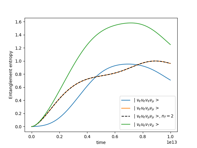
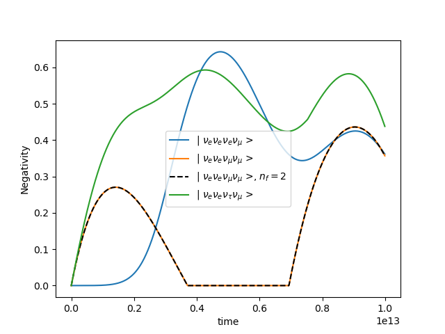
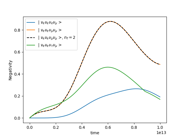
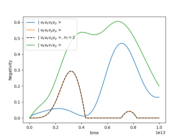
Figure 1: Under collective neutrino oscillations, time evolution of: entanglement entropy of the third neutrino (top), negativity between neutrinos 1 and 3 (bottom left), negativity between neutrinos 2 and 3 (bottom middle), and negativity between neutrinos 3 and 4 (bottom right). The terms in the $\nu$-$\nu$ interaction term of the Hamiltonian are given by Tab. 1. Number of neutrinos in the simulation, N, is 4 and number of neutrino-flavors, $n_{f}$, is 3. The purple icon at the top-right indicates exact simulation on a classical device [134].

The results for an initial state of $\ket{\nu_{e}\nu_{e}\nu_{\tau}\nu_{\mu}}$ with Hamiltonian parameters in Tab. 1 were replicated on Advantage. Nine different times were sampled, and the following procedure was used for each time: The initial state would be transformed into the mass-basis and split into blocks, each of which is composed of all mass-basis states with a given number of neutrinos in each mass-basis eigenstate. For N = 4 and $n_{f}$ = 3, there are 3 blocks of size 1, 6 blocks of size 4, 3 blocks of size 6, and 3 blocks of size 12. Time-evolution using the techniques outlined in Sec. III would be done separately for each block. In the event of a nonconvergence, defined as the previous 8 iterations achieving a percentage difference of less than 1% between the expectation values of the Feynman clock Hamiltonian obtained from Eq. 11 from adjacent iterations, the digitization would be rewound to the last iteration at which the progression of the Feynman clock expectation value was consistent with that of converging samples and would begin again from that point. The results from each block would be put back together to form the result for the state-vector, from which the entanglement entropy and negativity would then be extracted. The results for the “probe” third neutrino are seen in Fig. 2. All results are enumerated in App. C. Successful convergence to the classical result was achieved on Advantage to classical machine precision without Trotter error, similar to what was accomplished in Ref. [77]. In addition, the natural block-diagonalization of the neutrino mass basis was demonstrated to be a promising avenue for extending the reach of quantum simulation of $\nu$-$\nu$ interaction.

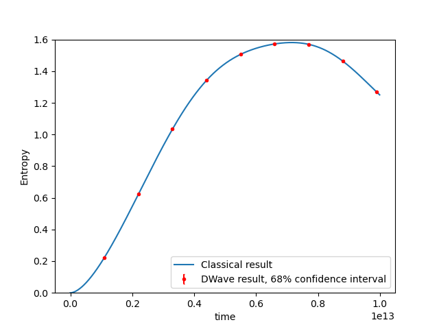
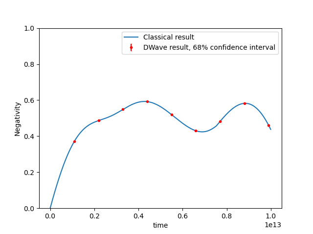
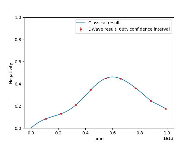
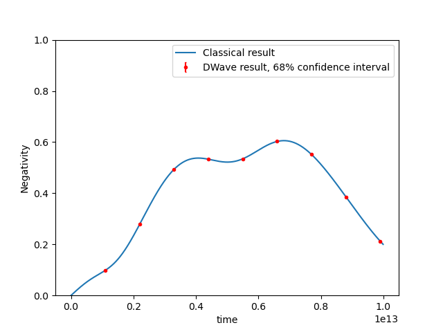
Figure 2: A comparison of an N = 4, $n_{f}$ = 3 collective neutrino oscillation results from Advantage and exact classical computation for entanglement entropy of the third (“probe”) neutrino (top), negativity between neutrinos 1 and 3 (bottom left), negativity between neutrinos 2 and 3 (bottom middle), and negativity between neutrinos 3 and 4 (bottom right). The initial state is $\ket{\nu_{e}\nu_{e}\nu_{\tau}\nu_{\mu}}$ and the Hamiltonian parameters are given by Tab. 1. The blue icon at the top-right indicates simulation on a quantum device [134].

V Attempts at quantum scaling advantage

The mapping of the collective neutrino oscillation system to a QUBO problem solvable on the annealer scales linearly with the size of the system’s Hilbert space. This is the same level of performance attainable with a classical device. Hence, in order to obtain a quantum advantage, a different approach is needed.

In principle, it may be possible to create a Hamiltonian whose ground state will provide the desired observable’s value for a given initial state. However, doing this efficiently would require the mapping of both the time evolution and the measurement process onto a matrix that would scale linearly (or at least polynomially) in dimensions with system size. This may be possible for a few specific cases, but if one can do this in general, then that would raise the question of why it cannot be done on a classial device. One key difficulty is the one of representation of entanglement. Neither the ground state of the annealer’s $H_{i}$ nor the bitstrings that the annealer is designed to return can reflect entanglement.

V.1 Scalable qubit-mapping

The first place examined for scalability is the number of states that a device designed to anneal to Eq. 4 can produce. The full state of $N_{q}$ qubits would have $2^{N_{q}}$ amplitudes, each of which would need a register of K bits to represent on a on a classical device, where K is the digitzation-factor from Eq. 7, which is set so that the precision of the amplitudes is $2^{-{K-1}}$. The number of states representable through this process is $2^{K2^{N_{q}}}$. For comparison, a classical device can represent $2^{N}$ possible states, where N is the number of bits on the device. Hence, the goal of quantum advantage in representable states is defined for the purposes of this project as the ability to represent O($2^{2^{N_{q}}}$) states with $O(N_{q})$ resources.

The only method of finding states other than the classical $2^{N_{q}}$ bitstrings on D-Wave’s Advantage annealer found during this project is to set the coefficients $h_{i}$ and $J_{ij}$ in Eq. 4 so that multiple bitstrings have the ground-state energy. One basic example would be where for a certain $i$, $h_{i}=0$ and $J_{ij}=0$ for all $j$. In this case, the state of the $i^{th}$ qubit would be $\frac{1}{\sqrt{2}}(\ket{\uparrow}-\ket{\downarrow})$. The range of states obtainable with this method is discrete: one state per set of bitstrings tied for the minimal energy. In principle, it is possible to obtain a $2^{2^{N_{q}}}-1$ scaling in this way if all possible combinations of bitsrtings are obtainable.

There are several challenges to this method. First, the number of parameters submittable to the Ising model is $\frac{1}{2}(n^{2}+n)$ for an n-qubit system. With the number of bitstrings scaling as $2^{n}$, this creates the possibility that a significant portion of bitstring combinations do not have a corresponding set of parameters that fix the entire combination to the ground state. Even if this does not come to pass, a map of $O(2^{2^{N_{q}}})$ Ising parameter-values to their corresponding states that is usable without exponentially scaling the classical resources needed to store and utilize said map will need to be found.

Second, making the energies of multiple bitstrings the same requires fine-tuning of the coefficients submitted to the machine. This reduces the precision of the anneal. This was confirmed using the Julia simulated quantum annealing library QuantumAnnealing.jl. QuantumAnnealing.jl simulates the perfect anneal of the Hamiltonian in Eq. 4 on a classical device [135]. Several simulated anneals were performed for an anneal-time of 1000 ns for systems of 2 qubits, after which $<\sigma^{(z)}>$ is taken for the first qubit. It was found that for parameters producing states obtainable from $\ket{-}\otimes\ket{-}$ using Clifford gates (which included the straightforwardly-obtainable bitstrings), the amplitudes were precise to 12 or more decimal places, while for other states the amplitudes were only precise to 4 decimal places. Similar results were obtained for simulations with the same anneal-time for 3-qubit systems. Advantage is sufficiently noisy that the procedure in Sec. IV and App. B requires hundreds of shots and maximizing the magnitude of the parameters that fix the ground state in order to produce one shot whose result is good enough to lead to convergence when running AQAE. With such noisy hardware, an anneal to a Hamiltonian with with multiple bitstrings at the ground-state energy will likely be unworkable due to the sensitivity of such a system.

Third, the coherence time of Advantage, which is $\approx$30 ns [136], is lower than even the lowest possible anneal-time that annealer users can access, which is 100 ns [119]. In principle, because the method above relies on superposition of bitstrings it could work despite this challenge. However, the processes intended to arrive at or do complex tomography on the correct state would still likely experience substantial noise from this decoherence.

V.2 Measurement-based quantum computing

It happens that the classical Ising model Hamiltonian, $H_{f}$, that Advantage anneals to is the same as the Hamiltonian that can be used to obtain a cluster state for measurement-based quantum computing from the state $\ket{+}\otimes\ket{+}\otimes\ldots\otimes\ket{+}$ [137]. Since this Hamiltonian is composed of a sum of Pauli strings that are constructed entirely out of identity and $\sigma^{z}$ operators, it can be adapted to do the same transformation for an initial state of $\ket{-}\otimes\ket{-}\otimes\ldots\otimes\ket{-}$ by adding a term proportional to $\frac{\pi}{2}\sigma^{z}_{i}$ for each qubit $i$. Thus, one can obtain such a cluster state by starting an anneal and suddenly changing the parameters $A(s)$ and $B(s)$ in Eq. 4 from $A(s)=1$, $B(s)=0$ to $A(s)=0$, $B(s)=1$ and evolving for long enough.

An arbitrary $SU(2)$ rotation can be written in terms of Euler angles, $U_{rot}(\theta,\phi,\xi)=U_{x}(\theta)U_{z}(\phi)U_{x}(\xi)$. It can then be implemented using measurement-based quantum computing by evolving a chain of five qubits, one with the initial state $\ket{\psi_{i}n}$ and the other four in the state $\ket{+}$ (or $\ket{-}$), using the cluster-state creation Hamiltonian mentioned previously. Then, Qubits 1-4 could be measured in the basis

$$B(\phi)=\{\frac{\ket{0}+e^{i\phi}\ket{1}}{\sqrt{2}},\frac{\ket{0}-e^{i\phi}\ket{1}}{\sqrt{2}}\}$$ (16)

where $\phi$ is 0, $\theta$, $\phi$, and $\xi$ for Qubits 1, 2, 3, and 4, respectively [137]. Qubit 5 would then be in the state $U_{rot}(\theta,\phi,\xi)\ket{\psi_{i}n}$, aside from some measurement-dependent corrections that can be done once the entire circuit is done and the final measurement results are obtained. The CNOT gate can be obtained in MBQC via measurements in the X and Y basis. Hence, a complete quantum computing basis can be obtained by measuring the qubits in a cluster state in basis lying on the equator of the Bloch sphere [137].

To implement this on Advantage, an extra rotation of $e^{i\sigma^{z}\omega}$, where $\omega$ is the clockwise (as viewed from the +z direction) angle between the measurement axis and the positive Y-axis, would be applied to each qubit via an adjustment of the tunable Ising Hamiltonian. Then, a rotation of $e^{i\frac{\pi}{2}\sigma^{x}}$ would be applied after suddenly switching the system back to $A(s)=1$, $B(s)=0$.

There are several challenges to this approach as well. First, the minimum execution time for Advantage to execute the sudden transition, or quench, required by this process is 100 ns [119]. This imperfect sudden transition could be a source of error. The second challenge is the high level of noise and short decoherence time. Third, Trotter-error-free time evolution is generally not possible with this method, as it works by encoding the conventional gate-based quantum computing onto a quantum annealer.

VI Other systems

VI.1 Neutrino-antineutrino oscillations

In the literature discussed in Section I surrounding neutrinos in the early Universe, neutron star mergers, and core-collapse supernovae, antineutrinos play as important of a role as neutrinos. Hence, in the interest of a complete physical picture, it is important to devise methods of simulating mixtures of neutrinos and antineutrinos. Neutrino-antineutrino interaction is not included in Eq. 1 but is straightforward to reproduce. The Hamiltonian can be re-written in terms of neutrino creation and annihilation operators. The neutrino creation operator can then be set equal to the antineutrino annihilation operator and vice versa. Besides this change, the neutrino-antineutrino interaction picks up an additional factor of -2 [104]. This is because a neutrino and an antineutrino are distinguishable by virtue of being a particle and an antiparticle, as opposed to simply being two particles of the same type. By doubling the number of interaction-permutations, this doubles the amplitude of the interaction [138]. The change-of-sign happens because the Feynman diagrams for neutrino-antineutrino interactions are odd permutations of those for neutrino-neutrino interactions [138]. The resulting additional term for neutrino-antineutrino interactions is as follows:

$$H_{\nu\bar{\nu}}=-2\sum_{p,p^{{}^{\prime}}}k(1-\cos{\theta_{pp^{{}^{\prime}}}})\vec{\lambda}^{*}_{p}\cdot\vec{\lambda}_{p^{{}^{\prime}}}$$ (17)

where $p^{{}^{\prime}}$ must index an antineutrino mode if $p$ indexes a neutrino mode and must index a neutrino mode if $p$ indexes an antineutrino mode. The superscript asterisk denotes complex conjugation. Physically, the neutrino-antineutrino interactions in Eq. 17 correspond to a neutrino and an antineutrino annihilating, forming a Z-boson, and creating a neutrino-antineutrino pair. Neutrinos and antineutrinos simply annihilating into Z-bosons or neutrino-antineutrino pairs being created out of W- and Z-bosons are not considered here, because neutrino energies considered here are 10 MeV, 3 orders of magnitude below the rest mass of W- and Z- bosons. In principle, it is also possible for a neutrino and an antineutrino to exchange momentum via a Z-boson. However, a recent study found that such interactions are helicity-suppressed. That is, they are nonexistent in the limit of massless neutrinos and in the physical reality are negligibly small given the small mass of neutrinos [139]. Hence, Eq. 17 fully encapsulates a neutrino-antineutrino system’s interactions to a very good approximation.

One marked difference between the neutrino-neutrino and neutrino-antineutrino systems is that unlike for the former, the 2-body interaction is not independent of the basis that the neutrinos are in for the latter. Hence, the full Hamiltonian for the neutrino-antineutrino term must be written with the single-neutrino terms in the flavor basis. For $n_{f}$=3, for example:

$$H^{\nu\bar{\nu}}_{CNO}=\sum_{p=1}^{N}{U_{PMNS}}_{p}\vec{B}\cdot\vec{\lambda}_{p}{U_{PMNS}^{\dagger}}_{p}-2\sum_{p,p^{{}^{\prime}}}k(1-\cos{\theta_{pp^{{}^{\prime}}}})\vec{\lambda}^{*}_{p}\cdot\vec{\lambda}_{p^{{}^{\prime}}}$$ (18)

with ${U_{PMNS}}_{p}$ and ${U_{PMNS}^{\dagger}}_{p}$ representing the PMNS matrix applied to the neutrino or antineutrino mode indexed by $p$. Additionally, the 2-body interaction does not commute with the single-neutrino oscilation term, so the reasoning behind the treatment of $\vec{B}$ as arbitrary in Sec. IV no longer holds. Hence, $\vec{B}$ is fixed to $(0,0,-\frac{\delta m^{2}}{4E},0,0,0,0,-\frac{\Delta m^{2}}{2\sqrt{3}E})$, the value obtained in App. A.

Because the interaction term represented by Eq. 17 is not basis-independent and is specific to the flavor basis, the domain-decomposition technique used in Sec. IV to place interacting N = 4 neutrino systems on Advantage cannot be used for neutrino-antineutrino systems. This limits the reach of quantum annealers in simulations of mixtures of neutrinos and antineutrinos. It is still, however, interesting to explore the physics collective neutrino-antineutrino oscillations using exact classical simulations.

Fig. 3 shows a comparison of results for the time evolution of entanglement entropy obtained using exact linear algebra on a classical computer for four systems with N = 2 neutrinos, one for each of the following initial states: $\ket{\nu_{e}\nu_{e}}$, $\ket{\nu_{e}\nu_{\mu}}$, $\ket{\nu_{e}\bar{\nu}_{e}}$, $\ket{\nu_{e}\bar{\nu}_{\mu}}$. N = 2 was chosen in order to sample the phenomenon of annihilation and re-creation of one neutrino-antineutrino pair in isolation. Each two-body system is analyzed for both $n_{f}$ = 2 and $n_{f}$ = 3. The neutrino-neutrino systems show no difference between the $n_{f}$ = 2 and $n_{f}$ = 3 results. However, for the neutrino-antineutrino systems, there is a difference: for $n_{f}$ = 3, the neutrino-antineutrino entanglement entropies are more irregular. The $\ket{\nu_{e}\bar{\nu}_{\mu}}$ system in particular shows non-periodic behavior, reminiscent of the Second Law of Thermodynamics, whereby there is a general trend towards the maximum entropy of $log_{2}(3)$. Changing the physics to set all mixing angles to zero, or setting all mixing angles but $\theta_{v12}$ and one of the mass-difference parameters to 0, are the only ways to make it so that the $n_{f}$ = 2 neutrino-antineutrino result replicates the $n_{f}$ = 3 neutrino-antineutrino result. Physically, this suggests that another neutrino flavor inaccessible through neutrino oscillation but accessible through neutral current would be detectable through neutrino-antineutrino interactions as long as the mass of the new eigenstate does not equal the mean of the previous eigenstates’ masses.

A similar analysis, shown in Fig. 4, was done for the case where only the neutrino-neutrino and neutrino-antineutrino interaction was kept, which would be a good approximation for the case immediately at the neutrinosphere, the part of the proto-neutron star from where the neutrinos stream into the outer layers from [140]. In this scenario, only initial states of $\ket{\nu_{e}\nu_{\mu}}$ and $\ket{\nu_{e}\bar{\nu}_{e}}$ produce entanglement. $\ket{\nu_{e}\bar{\nu}_{e}}$’s entanglement oscillations for $n_{f}$ = 3 have $\frac{3}{4}$ of the frequency of, experience a bimodal character not present in, and have a higher maximum ($log_{2}(3)$ vs 1) than corresponding oscillations for $n_{f}$ = 2. This $n_{f}$ = 3 bimodal behavior may be what manifests in more complex behavior when the single-neutrino oscillation is present. For $n_{f}$ = 2, frequency is twice that if single-neutrino oscillation was present, but other than that the entanglement dynamics are the same as for the neutrino-neutrino case.

VI.2 Majorana Neutrinos

All of the work discussed so far assumes that neutrinos are Dirac fermions. However, there are theories that stipulate that neutrinos are either Majorana fermions or have a Majorana mass [141]. For Majorana neutrinos, the creation and annihilation operators are identical [142]. Recent studies have suggested that the Majorana nature of neutrinos can manifest itself in signatures of the neutrino magnetic moment [143] and neutrino spin-flavor precession [144, 145] in environments where collective neutrino oscillations are present. To see if Majorana effects are visible for entanglement observables, the N = 2 simulations done in Sec. VI.1 are repeated for Majorana fermions.

As formulated by Steven Weinberg in the 1970s, the five-dimensional Standard Model can include the following term:

$$\mathcal{L}_{Weinberg}=f_{abmn}\bar{l}^{C}_{iaL}l_{jbL}\phi^{(m)}_{k}\phi^{(n)}_{l}\epsilon_{ik}\epsilon_{jl}+f_{abmn}^{{}^{\prime}}\bar{l}^{C}_{iaL}l_{jbL}\phi^{(m)}_{k}\phi^{(n)}_{l}\epsilon_{ij}\epsilon_{kl}$$ (19)

where $f_{abmn}$ and $f_{abmn}^{{}^{\prime}}$ are coefficients with a magnitude on the order of $\frac{1}{M}$ with M being a characteristic mass above approximately $10^{14}$ GeV of hypothetical ’superheavy’ particles, $l_{jbL}$ is the $j^{th}$ component of the vector in the fundamental representation of SU(2) representing a non-conserved lepton (in this case, a neutrino) with flavor $b$ with left-handed chirality, the superscript ${C}$ denotes charge-conjugation, and $\phi^{(m)}_{k}$ is a scalar field that the Higgs field can be substituted in for [146]. On a staggered lattice, where each spatial lattice site $i$ is split into two sites, $l$ for neutrinos and $l^{{}^{\prime}}$ for antineutrinos, $\mathcal{L}_{Weinberg}$ can be converted into a Hermitian Hamiltonian form, like so:

$$H^{Majorana}_{m}=\frac{1}{2}m_{M}\sum_{i}(a_{il}a_{il^{{}^{\prime}}}+a^{\dagger}_{il}a^{\dagger}_{il^{{}^{\prime}}})$$ (20)

with $a$ and $a^{\dagger}$ being creation and annihilation operators for the neutrino or antineutrino that exists on the staggered lattice site denoted by its subscript, with the creation operator for neutrinos being the annihilation operator for antineutrinos and vice versa. This term produces a “Majorana mass” $m_{M}$ for the neutrinos [147].

For a single-spatial-site lattice localized to spatial site $i$, the eigenstate of $H^{Majorana}_{m}$ which has a “mass” of $m_{M}$ is $\frac{\ket{\nu}+\ket{\bar{\nu}}}{\sqrt{2}}$, that is, an equal superposition of there being one neutrino on the spatial lattice site and there being one antineutrino on the spatial lattice site. This state can be interpreted as the projection of a Majorana neutrino onto the Dirac neutrino state-space used so far in this work. From this fact, one can obtain the interaction of any pair of Majorana neutrinos through direct addition of the two-neutrino term in Eq. 1 and its counterpart for antineutrino-antineutrino interactions (which is the same [104]) to the neutrino-antineutrino interaction term in Eq. 17. The resulting collective neutrino oscillation Hamiltonian for Majorana neutrinos is as follows:

$$H^{majorana}_{\nu\nu}=\sum_{p}{U_{PMNS}}_{p}\vec{B}\cdot\vec{\lambda}_{p}{U_{PMNS}^{\dagger}}_{p}+2*\sum_{p,p^{{}^{\prime}}}k(1-\cos{\theta_{pp^{{}^{\prime}}}})Im(\vec{\lambda}_{p})\cdot Im(\vec{\lambda}_{p^{{}^{\prime}}})$$ (21)

where Im() denotes the imaginary component. Similar to the neutrino-antineutrino oscillation, the two-body interaction term is not invariant with a change of basis, so $\vec{B}$ is fixed to the same value as in Sec. VI.1. Fig. 3 shows results for Majorana neutrinos. The $n_{f}$ = 3 case shows more irregularity than the $n_{f}$ = 2 case, with the $\ket{\nu_{e}\bar{\nu}_{\mu}}$ initial state showing non-periodic behavior. Also similar to the neutrino-antineutrino case, changing the physics to set all mixing angles to zero, or to set all mixing angles but $\theta_{v12}$ and one of the mass-difference parameters to 0, are the only ways to make it so that the $n_{f}$ = 2 neutrino-antineutrino result replicates the $n_{f}$ = 3 neutrino-antineutrino result. One difference is that lower-amplitude, higher-frequency modes have a lower prominence for the $\ket{\nu_{e}\nu_{e}}$ initial state and a higher prominence for the $\ket{\nu_{e}\nu_{\mu}}$ initial state than for Dirac neutrino-antineutrino and neutrino-neutrino counterparts, respectively. Additionally, the frequency of the oscillation for periodic patterns is half that of counterparts in the Dirac case. If this result holds for asymptotically large N, this suggests that neutrinos from the initial burst at the collapse of an iron core, which is probably composed primarily of electron neutrinos, could potentially be used to probe whether neutrinos are Majorana or Dirac fermions. For the interaction-term-only case shown in Fig. 4, the results the same as those of the Dirac neutrino case for the initial state of $\ket{\nu_{e}\nu_{\mu}}$.

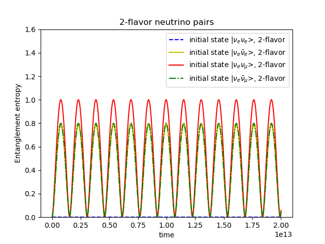
Figure 3: Top: A comparison, which assumes the neutrinos are Dirac particles, of 2-neutrino and 1 neutrino-1 antineutrino (both N = 2) systems’ entanglement entropy evolution. $n_{f}$ = 2 is in the left, $n_{f}$ = 3 is on the right. Bottom: an analogous comparison for Majorana neutrinos. Parameters are shown in Tab. 1. The purple icon at the top-right indicates exact simulation on a classical device [134].

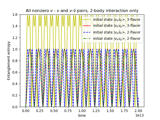
Figure 4: A comparison of Dirac and Majorana N= 2 neutrino systems’ entanglement entropy evolution for $n_{f}$ = 2 and $n_{f}$ = 3, representative of all scenarios that produce nonzero results. Parameters are the same as those in Tab. 1. The purple icon at the top-right indicates exact simulation on a classical device [134].

VI.3 Time-dependent Hamiltonian

As mentioned at the beginning of Section II, time-dependence of neutrino-neutrino interaction, despite being physical, is excluded from this study in order to facilitate algorithm-development on the quantum annealer. With a time-independent Hamiltonian, expession of the time-evolution in the form of a QUBO matrix is a straightforward use of the time-evolution operator, $e^{-iHt}$. However, for a time-dependent Hamiltonian, the time-evolution operator is the time-ordered integral [138],

$$T(e^{-i\int_{t_{i}}^{t_{f}}H(t)dt})$$ (22)

Thus, the use of the same techniques with a time-dependent Hamiltonian would result in an error in the calculation determined by a continuum limit of the Zassenhaus formula [148, 149],

$$e^{t(X+Y)}=e^{tX}e^{tY}e^{-\frac{t^{2}}{2}[X,Y]}e^{-\frac{t^{3}}{6}(2[Y,[X,Y]]+[X,[X,Y]])}e^{-\frac{t^{4}}{24}([[[X,Y],X],X]+3[[[X,Y],X],Y]+3[[[X,Y],Y],Y])}\cdots$$ (23)

which removes one of the main advantages of using a quantum annealer, which is the avoidance of Trotter errors. It is possible to avoid these Trotter errors, but that would require the Schrödinger equation to be fully solved in order to represent the time evolution in QUBO form, which is sufficient to find the time evolution by itself.

VII Conclusion

This work presents results for multi-angle, three-flavor collective neutrino oscillation time evolution on a quantum device and successful verification using exact numerical calculations. Interactions of neutrino-antineutrino and Majorana neutrino pairs are also investigated. Following the direction of Ref. [77], the Feynman Clock method was used to encode the time-evolution of a collective neutrino oscillation system onto a Hamiltonian whose ground state equals a concatenation of the initial and final state of that time evolution. The Adaptive Quantum Annealing Eigensolver (AQAE) method was then used to obtain said states to classical machine precision on the Advantage quantum annealer.

Simulating four neutrinos that each have three possible flavors required the use of domain-decomposition in order to fit on the limited number of logical qubits available, which was accomplished by taking advantage of the fact that in the mass-basis, the collective neutrino oscillation Hamiltonian is naturally block diagonalized to utilize domain-decomposition. This technique is only possible with a neutrino-neutrino interaction that is invariant with respect to neutrino-basis transformation under the Pontecorvo–Maki–Nakagawa–Sakata (PMNS) matrix. Therefore, while it works for systems of Dirac neutrinos, it does not work for neutrino-antineutrino mixtures or for Majorana neutrinos and other schemes would be required in order to implement block-diagonalization for these systems.

Just like in Ref. [77], AQAE on the quantum annealer can reproduce time evolution without Trotter errors, but does so with a scaling that is not any better than that of classical devices. Addressing this challenge faces multiple obstacles. First, the number of possible ground states of Advantage’s $H_{f}$ from Section III scaling quadratically (rather than exponentially) with system size. Thus, it will likely take annealers with alternative choices of $H_{\alpha}$ (in Section III’s parlance), such as the ZZXX and the ZX Hamiltonian [150, 151], for quantum annealing to see the scaling advantage of conventional gate-based qubit devices. It is theoretically possible to obtain an exponential improvement in scaling on Advantage, by utilizing its $H_{\alpha}$ to implement measurement-based quantum computing. However, this procedure relies on instantaneous quenches between $H_{i}$ and $H_{f}$. In practice, state-of-the-art annealers take time to quench, creating a source of error. Also, Trotter errors will still be present in this implementation. This is in addition to decoherence errors, which are inevitable, as the decoherence time of Advantage, $\approx$30 ns, is shorter than any anneal-time available on the device. Finally, the available quantum advantage algorithms are less resilient to noise than annealing to a bit-string.

D-Wave Inc.’s new Advantage2 annealer has more qubits, longer coherence time ($\approx$300 ns compared to Advantage’s $\approx$30 ns), and less noise than Advantage [152]. Hence, it is possible that paths toward quantum advantage on annealers could be explored on Advantage2 and its successors. However, with the advent of gate-based devices with thousands of qubits, such as IBM’s Condor processor [153], it will likely be more promising to use gate-based quantum computing for time evolution and to use quantum annealers for optimization problems.

Since it is entanglement that serves as the determiner of where problems that are inefficient to solve with a classical device but efficient to solve with a quantum device lie, the time-evolution data is expressed in terms of entanglement witnesses. For the case of a pure Dirac neutrino sample without antineutrinos, I have found that the entanglement dynamics of neutrinos with the physical number of flavors ($n_{f}$) of 3 are different from what can be produced by an $n_{f}$ = 2 system if and only if all three neutrino flavors are present in the initial state. This suggests that for a near purely $\nu_{e}$ sample, which is likely a close approximation of the composition of the neutrinos first emitted as the iron core of a massive star collapses [24, 25, 26], relevant three-flavor dynamics can be simulated efficiently on classical computers with methods such as mean field theory, while any entangling phenomena can be obtained using a two-flavor simulation. This is in contrast to results from Ref. [68], which showed a difference in results between two-flavor and three-flavor models for a system whose initial state is entirely composed of electron neutrinos.

Three possible explanations for this apparent discrepancy are that (1) a two-flavor model not considered in Ref. [68], perhaps with a different mixing angle or mass difference parameter, could accurately reflect three-flavor dynamics of an initially pure-electron-neutrino system, (2) a difference between two-flavor and three-flavor dynamics manifests itself in initially pure-electron-neutrino systems when either time-dependent neutrino-neutrino interactions or neutrinos with different momentum magnitudes enter the picture, or (3) the difference found in Ref. [68] does not affect entanglement.

However, if physical neutrinos are Majorana fermions, then the findings of this work suggest a far different outcome. Even for the simple case where the number of neutrinos, N, is 2, Majorana neutrino entanglement show a marked difference in behavior from $n_{f}$ = 2 to $n_{f}$ = 3 for all initial states. This result indicates that the entanglement structure of the initial burst of electron neutrinos from the core-collapse of a massive star can potentially indicate if neutrinos exhibit a Majorana mass or not. Thus, the behavior of collective Majorana neutrino oscillations in larger systems and their effects on supernova observables are a potential next step.

O(1 second) after core collapse, the neutrinos from the core are expected to be a roughly even mixture of all three flavors and of neutrinos and antineutrinos [24, 25, 26]. For such a system, I have found that $n_{f}$ = 3 entanglement dynamics are distinct from those for $n_{f}$ = 2. This is due to two reasons. The first is the difference with $n_{f}$ = 2 behavior exhibited by a state that starts as a mixture of all three flavors. The second is because, similar to Majorana neutrinos, neutrino-antineutrino mixtures show substantial differences between $n_{f}$ = 2 and $n_{f}$ = 3 even for the simple N = 2 case. This finding is analogous to the results in Ref. [55] for tensor network methods using the time-dependent variational principle (TDVP). In Ref. [55], it was found that resource-scaling of TDVP is significantly worse for mixtures of neutrino flavors than for an all-$\nu_{e}$ sample. In conclusion, a simulation of larger-N neutrino-antineutrino mixtures with all three flavors equally represented could be an ideal substrate for realizing quantum advantage and for a characterization of the features of $n_{f}$ = 3 similar to what Refs. [44, 45, 46, 47, 48, 49, 50, 52, 53, 54, 56, 57, 58, 59] found for $n_{f}$ = 2.

Appendix A Derivation of the $n_{f}$ = 3 single-neutrino oscillation Hamiltonian term

First, assuming that the velocity, and hence the momentum of all 3 mass-eigenstates of the neutrino are the same, and expressing each eigenstate’s energy using the relativistic energy formula, the Hamiltonian is as follows:

$$H_{\nu}=\sqrt{m_{1}^{2}+p^{2}}\ket{1}\bra{1}+\sqrt{m_{2}^{2}+p^{2}}\ket{2}\bra{2}+\sqrt{m_{3}^{2}+p^{2}}\ket{3}\bra{3}$$ (24)

In the ultrarelativistic limit, which neutrinos with energies of 10 MeV can be approximated to be in, one can take the Taylor expansion of the square root function around the zero-mass limit:

$$H_{\nu}=p(1+\frac{m_{1}^{2}}{2p^{2}})\ket{1}\bra{1}+p(1+\frac{m_{2}^{2}}{2p^{2}})\ket{2}\bra{2}+p(1+\frac{m_{3}^{2}}{2p^{2}})\ket{3}\bra{3}$$ (25)

Because the zero-point of energy is arbitrary, I can simply subtract the identity matrix times $(p+\frac{m_{1}^{2}+m_{2}^{2}+m_{3}^{2}}{6p^{2}})$ to make the Hamiltonian traceless:

$$H_{\nu}=\frac{2m_{1}^{2}-m_{2}^{2}-m_{3}^{2}}{6p}\ket{1}\bra{1}+\frac{2m_{2}^{2}-m_{1}^{2}-m_{3}^{2}}{6p}\ket{2}\bra{2}+\frac{2m_{3}^{2}-m_{1}^{2}-m_{2}^{2}}{6p}\ket{3}\bra{3}$$ (26)

Defining $\delta m^{2}=m_{2}^{2}-m_{1}^{2}$ and $\Delta m^{2}=m_{3}^{2}-\frac{m_{2}^{2}+m_{1}^{2}}{2}$, we can get

$$H_{\nu}=\frac{-\frac{3}{2}\delta m^{2}-\Delta m^{2}}{6p}\ket{1}\bra{1}+\frac{\frac{3}{2}\delta m^{2}-\Delta m^{2}}{6p}\ket{2}\bra{2}+\frac{\Delta m^{2}}{6p}\ket{3}\bra{3}$$ (27)

And given that in the ultrarelativistic limit, $p\simeq E$,

$$H_{\nu}=(-\frac{\delta m^{2}}{4E}-\frac{\Delta m^{2}}{6E})\ket{1}\bra{1}+(\frac{\delta m^{2}}{4E}-\frac{\Delta m^{2}}{6E})\ket{2}\bra{2}+(\frac{\Delta m^{2}}{3E})\ket{3}\bra{3}$$ (28)

Or:

$$H_{\nu}=-\frac{\delta m^{2}}{4E}\lambda_{3}-\frac{\Delta m^{2}}{2\sqrt{3}E}\lambda_{8}$$ (29)

Appendix B Benchmarking

AQAE’s performance depends on the number of repetitions of the anneal, the annealing time, and the constants K and z in Eq. 10 and 12 which determine the digitization and the number of zoom-steps. Thus, the first step before running any process on the annealer is to use D-Wave’s simulated classical thermal annealer, neal, to assess the best way to use these parameters to optimize device performance. The Hamiltonian in Eq. 1 was used in this case, with N = 2. The parameters are the same ones in Tab. 1.$\vec{B}$ was simply taken from Ref. [68]: $\vec{B}=(0,0,-\frac{\delta m^{2}}{4E},0,0,0,0,-\frac{\Delta m^{2}}{4E})$. The starting state was $\ket{\nu_{e}\nu_{\mu}}$. The time-increment evolved over was t = $10^{12}eV^{-1}$. The reverse-digitization process and the fixing of the penalty term $h_{i}$ values discussed in Section III were not used; instead, the digitization procedure and the penalty term were found in the same manner as in Ref. [77]. In doing so, I replicate Ref. [77]’s result that increasing z produces a much greater improvement in precision than any of the above options, as seen in Fig. 5.

Thus, K, anneal-time, and the number of repetitions of each anneal-step only need to be adequate to converge, and once that is assured, the way to improve precision is to increase z. The next step is to assess how many zoom-steps are needed in order to converge to a satisfactory precision. This was done by running the same simulation on Advantage, with the reverse-digitization and fixing of the penalty term $h_{i}$ values included. Annealer parameters were K = 2, anneal-time 5 $\mu s$, 1000 repetitions of each zoom-step, and a chain-strength of 1. As seen in Fig. 6, it takes about 26 zoom-steps to converge.

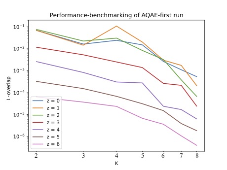
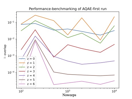
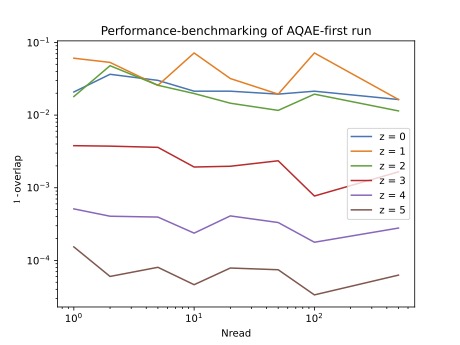
Figure 5: From left to right, the effect of z and K, of z and the number of sweeps in an anneal (which is a surrogate for anneal-time), and of z and the number of anneal-repetitions per call to the annealer on 1 minus the dot product of the final state-vector of the time-evolution of 2 neutrinos as calculated by Neal and the same state-vector as calculated using exact linear algebra. The initial state is $\ket{\nu_{e}\nu_{\mu}}$, the Hamiltonian used for the evolution is Equation 1, the parameters are found in Table 1, and the time-interval evolved over is $10^{12}$ $eV^{-1}$ . Each entry is the lowest-energy final result out of all the anneal-repetitions in its AQAE step. The yellow icon at the top-right indicates a noisy classical simulation [134].

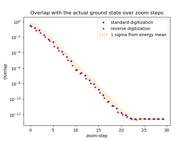
Figure 6: The overlap between results of time-evolution with AQAE of a three-flavor, two-neutrino system starting as one electron and one muon neutrino and evolved over a time-increment of $10^{10}eV^{-1}$ and the actual final state. $N_{reads}$ = 1000, $a_{t}$ = 20 $\mu s$, K = 1, and chain-strength = 1. The blue icon at the top-right indicates simulation on a quantum device [134].

Appendix C Tables of N = 4 $\nu$-$\nu$ results for entanglement witnesses

time ($eV^{-1}$)	$S_{3}(t)$
$1.1*10^{12}$	$0.222927229(^{+619}_{-1527})$
$2.2*10^{12}$	$0.623264640(^{+50}_{-3222})$
$3.3*10^{12}$	$1.0340534849(^{+1546}_{-660})$
$4.4*10^{12}$	$1.3420253885(^{+18009}_{-6643})$
$5.5*10^{12}$	$1.5060393872(^{+2875}_{-67})$
$6.6*10^{12}$	$1.5718841229(^{+252}_{-308})$
$7.7*10^{12}$	$1.5693430609(^{+6021}_{-1011})$
$8.8*10^{12}$	$1.4631204675(^{+109}_{-6577})$
$9.9*10^{12}$	$1.2671452598(^{+451}_{-54})$

Table 2: A table of the D-Wave Advantage quantum annealer results for entanglement entropy for the third neutrino of the N = 4, $n_{f}$ = 3 system results from Fig. 2. Error bars are 1$\sigma$ confidence intervals.

time ($eV^{-1}$)	$N_{13}(t)$	$N_{23}(t)$	$N_{34}(t)$
$1.1*10^{12}$	$0.3720986223(^{+10285}_{-17470})$	$0.0842779937(^{+2064}_{-9353})$	$0.0984672558(^{+4280}_{-16009})$
$2.2*10^{12}$	$0.4868408929(^{+104}_{-13601})$	$0.1291148436(^{+194}_{-692})$	$0.2787261578(^{+144}_{-4655})$
$3.3*10^{12}$	$0.5484990103(^{+712}_{-7655})$	$0.2091610157(^{+20706}_{-110})$	$0.4936497469(^{+94}_{-18696})$
$4.4*10^{12}$	$0.5918213991(^{+694}_{-5279})$	$0.3460545631(^{+2102}_{-12006})$	$0.5329880752(^{+7887}_{-255})$
$5.5*10^{12}$	$0.5197404555(^{+117}_{-1131})$	$0.4497961383(^{+364}_{-654})$	$0.5347131445(^{+495}_{-387e})$
$6.6*10^{12}$	$0.4301304886(^{+1428}_{-64})$	$0.4458340852(^{+35}_{-3029})$	$0.6025444696(^{+695}_{-33})$
$7.7*10^{12}$	$0.4824124333(^{+18476}_{-461})$	$0.3611637035(^{+388}_{-22517})$	$0.5514675837(^{+731}_{-19224})$
$8.8*10^{12}$	$0.5822152101(^{+371}_{-1104})$	$0.2461251687(^{+351}_{-5615})$	$0.3860333315(^{+438}_{-1888})$
$9.9*10^{12}$	$0.4597905236(^{+16}_{-956})$	$0.1754865412(^{+301}_{-18})$	$0.2120581628(^{+1237}_{-18})$

Table 3: A table of the D-Wave Advantage quantum annealer results for negativities for the third neutrino of the N = 4, $n_{f}$ = 3 system results from Fig. 2. Error bars are 1$\sigma$ confidence intervals.

References

- Janka et al. [2007] H.-T. Janka, K. Langanke, A. Marek, G. Martínez-Pinedo, and B. Müller, Theory of core-collapse supernovae, Progress in Particle and Nuclear Physics 57, 142 (2007).
- Mezzacappa [2020] A. Mezzacappa, Toward realistic models of core collapse supernovae: A brief review, in Proceedings of the International Astronomical Union, Symposium S362: The Predictive Power of Computational Astrophysics as a Discovery Tool, Vol. 16 (2020) pp. 215–227.
- Burrows and Vartanyan [2021] A. Burrows and D. Vartanyan, Core-collapse supernova explosion theory, Nature 589, 29 (2021).
- Fuller and Haxton [2023] G. M. Fuller and W. C. Haxton, Neutrinos in Stellar Astrophysics, in The Encyclopedia of Cosmology (World Scientific Series in Astrophysics, 2023) pp. 367–431.
- Foucart [2023] F. Foucart, Neutrino transport in general relativistic neutron star merger simulations, Living Reviews in Computational Astrophysics 9, 1 (2023).
- Ruffert et al. [1997] M. Ruffert, H.-T. Janka, K. Takahashi, and G. Schäfer, Coalescing neutron stars – a step towards physical models II. Neutrino emission, neutron tori, and gamma-ray bursts, Astronomy & Astrophysics 319, 122 (1997).
- Radice et al. [2018] D. Radice, A. Perego, S. Bernuzzi, and B. Zhang, Long-lived remnants from binary neutron star mergers, Monthly Notices of the Royal Astronomical Society 481, 3670 (2018).
- Nedora et al. [2021] V. Nedora et al., Numerical Relativity Simulations of the Neutron Star Merger GW170817: Long-term Remnant Evolutions, Winds, Remnant Disks, and Nucleosynthesis, The Astrophysical Journal 906, 98 (2021), 20pp.
- Bowers and Wilson [1982] R. Bowers and J. R. Wilson, Collapse of Iron Stellar Cores, The Astrophysical Journal 263, 366 (1982).
- Woosley et al. [1988] S. E. Woosley, P. A. Pinto, and L. Ensman, Supernova 1987a-Six weeks later, The Astrophysical Journal 324, 466 (1988).
- Turatto et al. [1998] M. Turatto et al., The Peculiar Type II Supernova 1997D: A Case for a Very Low Mass, The Astrophysical Journal 498, L129 (1998).
- Sollerman et al. [1998] J. Sollerman, R. J. Cumming, and P. Lundqvist, A Very Low Mass of in the Ejecta of SN 1994WA, The Astrophysical Journal 493, 933 (1998).
- Nicholl et al. [2020] M. Nicholl et al., An extremely energetic supernova from a very massive star in a dense medium, Nature Astronomy 4, 893 (2020).
- Smith et al. [2007] N. Smith et al., SN 2006gy: Discovery of the most luminous supernova ever recorded, powered by the death of an extremely massive star like Carinae, The Astrophysical Journal 666, 1116 (2007).
- Drake et al. [2010] A. J. Drake, S. G. Djorgovski, J. L. Prieto, A. Mahabal, D. Balam, R. Williams, M. J. Graham, M. Catelan, E. Beshore, and S. Larson, Discovery of the extremely energetic supernova 2008fz, The Astrophysical Journal Letters 718, L127 (2010).
- Chatzopoulos et al. [2011] E. Chatzopoulos, J. C. Wheeler, J. Vinko, R. Quimby, E. L. Robinson, A. A. Miller, R. J. Foley, D. A. Perley, F. Yuan, C. Akerlof, and J. S. Bloom, SN 2008am: A super-luminous Type IIn supernova, The Astrophysical Journal 729, 143 (2011).
- Rest et al. [2011] A. Rest et al., Pushing the boundaries of conventional core-collapse supernovae: The extremely energetic supernova SN 2003ma, The Astrophysical Journal 729, 88 (2011).
- Benetti et al. [2017] S. Benetti et al., The supernova CSS121015:004244+132827: a clue for understanding superluminous supernovae, Monthly Notices of the Royal Astronomical Society 472, 1538 (2017).
- Pagliaroli et al. [2009] G. Pagliaroli, F. Vissani, M. L. Costantini, and A. Ianni, Improved analysis of SN1987a antineutrino events, Astroparticle Physics 31, 163 (2009).
- Colgate and White [1966] S. A. Colgate and R. H. White, The Hydrodynamic Behavior of Supernovae Explosions, Astrophysical Journal 143, 626 (1966).
- Arnett [1966] W. Arnett, Gravitational collapse and weak interactions, Canadian Journal of Physics 44, 2553 (1966).
- Wilson [1985] J. R. Wilson, Supernovae and Post-Collapse behavior, in Numerical Astrophysics, edited by J. Centrella, J. M. LeBlanc, and R. Bowers (1985) p. 422.
- Bethe and Wilson [1985] H. A. Bethe and J. R. Wilson, Revival of a stalled supernova shock by neutrino heating, The Astrophysical Journal 295, 14 (1985).
- Fischer et al. [2012] T. Fischer, G. Martínez-Pinedo, M. Hempel, and M. Liebendörfer, Neutrino spectra evolution during protoneutron star deleptonization, Phys. Rev. D 85, 083003 (2012).
- Fischer et al. [2010] T. Fischer, S. C. Whitehouse, A. Mezzacappa, F.-K. Thielemann, and M. Liebendörfer, Protoneutron star evolution and the neutrino-driven wind in general relativistic neutrino radiation hydrodynamics simulations, A&A 517, A80 (2010).
- Hüdepohl et al. [2010] L. Hüdepohl, B. Müller, H.-T. Janka, A. Marek, and G. G. Raffelt, Neutrino Signal of Electron-Capture Supernovae from Core Collapse to Cooling, PRL 104, 251101 (2010).
- Qian et al. [1993] Y.-Z. Qian, G. M. Fuller, G. J. Mathews, R. W. Mayle, J. R. Wilson, and S. E. Woosley, Connection between Flavor Mixing of Cosmologically Significant Neutrinos and Heavy Element Nucleosynthesis in Supernovae, Physical Review Letters 71, 1977 (1993).
- Fröhlich et al. [2006] C. Fröhlich, G. Martínez-Pinedo, M. Liebendörfer, F.-K. Thielemann, E. Bravo, W. Hix, K. Langanke, and N. Zinner, Neutrino-Induced Nucleosynthesis of A 64 Nuclei: The p Process, Physical Review Letters 96, 142502 (2006).
- Grohs and Fuller [2016] E. Grohs and G. M. Fuller, The surprising influence of late charged current weak interactions on Big Bang Nucleosynthesis, Nuclear Physics B 911, 955 (2016).
- Just et al. [2015] O. Just, A. Bauswein, R. Ardevol Pulpillo, S. Goriely, and H.-T. Janka, Comprehensive nucleosynthesis analysis for ejecta of compact binary mergers, MNRAS 448, 541 (2015).
- Wanajo [2006] S. Wanajo, The rp-process in neutrino-driven winds, The Astrophysical Journal 647, 1323 (2006).
- Woosley et al. [1990] S. Woosley, D. Hartmann, R. Hoffman, and W. Haxton, The -process, Astrophysical Journal, Part 1 (ISSN 0004-637X), vol. 356, June 10, 1990, p. 272-301. Research supported by the Los Alamos National Laboratory and University of California. 356, 272 (1990).
- Roberts et al. [2010] L. Roberts, S. Woosley, and R. Hoffman, Integrated nucleosynthesis in neutrino-driven winds, The Astrophysical Journal 722, 954 (2010).
- Sasaki et al. [2017] H. Sasaki, T. Kajino, T. Takiwaki, T. Hayakawa, A. Balantekin, and Y. Pehlivan, Possible effects of collective neutrino oscillations in three-flavor multiangle simulations of supernova p processes, Physical Review D 96, 043013 (2017).
- Balantekin et al. [2023a] A. Balantekin, M. J. Cervia, A. V. Patwardhan, R. Surman, and X. Wang, Collective neutrino oscillations and heavy-element nucleosynthesis in supernovae: exploring potential effects of many-body neutrino correlations, arXiv preprint arXiv:2311.02562 (2023a).
- Duan [2011] H. Duan, The influence of collective neutrino oscillations on a supernova r process, Journal of Physics G: Nuclear and Particle Physics 38, 035201 (2011).
- Fuller et al. [1987] G. M. Fuller, R. W. Mayle, J. R. Wilson, and D. N. Schramm, Resonant Neutrino Oscillations and Stellar Collapse, The Astrophysical Journal 322, 795 (1987).
- Nötzold and Raffelt [1988] D. Nötzold and G. Raffelt, Neutrino dispersion at finite temperature and density, Nuclear Physics B 307, 924 (1988).
- Sigl and Raffelt [1993] G. Sigl and G. Raffelt, General kinetic description of relativistic mixed neutrinos, Nuclear Physics B 406, 423 (1993).
- Qian and Fuller [1995] Y.-Z. Qian and G. M. Fuller, Neutrino-neutrino scattering and matter-enhanced neutrino flavor transformation in supernovae, Physical Review D 51, 1479 (1995).
- Shalgar and Tamborra [2023] S. Shalgar and I. Tamborra, Do we have enough evidence to invalidate the mean-field approximation adopted to model collective neutrino oscillations?, Physical Review D 107, 123004 (2023).
- Bethe [1931] H. Bethe, Zur Theorie der Metalle, Zeitschrift für Physik 71, 205 (1931).
- Vidal [2003] G. Vidal, Efficient Classical Simulation of Slightly Entangled Quantum Computations, Physical review letters 91, 147902 (2003).
- Pehlivan et al. [2011] Y. Pehlivan, A. B. Balantekin, T. Kajino, and T. Yoshida, Invariants of collective neutrino oscillations, Physical Review D 84, 065008 (2011).
- Espinoza et al. [2013] C. Espinoza, C. Volpe, and D. Vaeaenaenen, Extended evolution equations for neutrino propagation in astrophysical and cosmological environments, Physical Review D 87, 113010 (2013).
- Pehlivan et al. [2014a] Y. Pehlivan, A. B. Balantekin, and T. Kajino, Neutrino magnetic moment, CP violation, and flavor oscillations in matter, Physical Review D 90, 065011 (2014a).
- Birol et al. [2018] S. Birol, Y. Pehlivan, A. B. Balantekin, and T. Kajino, Neutrino spectral split in the exact many-body formalism, Physical Review D 98, 083002 (2018).
- Cervia et al. [2019a] M. J. Cervia, A. V. Patwardhan, and A. B. Balantekin, Symmetries of Hamiltonians describing systems with arbitrary spins, International Journal of Modern Physics E 28, 1950032 (2019a).
- Cervia et al. [2019b] M. J. Cervia, A. V. Patwardhan, A. B. Balantekin, S. N. Coppersmith, and C. W. Johnson, Entanglement and collective flavor oscillations in a dense neutrino gas, Phys. Rev. D 100, 083001 (2019b).
- Patwardhan et al. [2019] A. V. Patwardhan, M. J. Cervia, and A. B. Balantekin, Eigenvalues and eigenstates of the many-body collective neutrino oscillation problem, Physical Review D 99, 123013 (2019).
- Rrapaj [2020] E. Rrapaj, Exact solution of multiangle quantum many-body collective neutrino-flavor oscillations, Physical Review C 101, 065805 (2020).
- Patwardhan et al. [2021] A. V. Patwardhan, M. J. Cervia, and A. B. Balantekin, Spectral splits and entanglement entropy in collective neutrino oscillations, Physical Review D 104, 123035 (2021).
- Roggero [2021a] A. Roggero, Dynamical phase transitions in models of collective neutrino oscillations, Physical Review D 104, 123023 (2021a).
- Roggero [2021b] A. Roggero, Entanglement and many-body effects in collective neutrino oscillations, Physical Review D 104, 103016 (2021b).
- Cervia et al. [2022] M. J. Cervia, P. Siwach, A. V. Patwardhan, A. B. Balantekin, S. N. Coppersmith, and C. W. Johnson, Collective neutrino oscillations with tensor networks using a time-dependent variational principle, Physical Review D 105, 123025 (2022).
- Lacroix et al. [2022a] D. Lacroix, A. B. Balantekin, M. J. Cervia, A. V. Patwardhan, and P. Siwach, Role of non-Gaussian quantum fluctuations in neutrino entanglement, Physical Review D 106, 123006 (2022a).
- Martin et al. [2023] J. D. Martin, A. Roggero, H. Duan, and J. Carlson, Many-body neutrino flavor entanglement in a simple dynamic model, (2023), arXiv:2301.07049 [hep-ph] .
- Cirigliano et al. [2024] V. Cirigliano, S. Sen, and Y. Yamauchi, Neutrino many-body flavor evolution: the full Hamiltonian, arXiv preprint arXiv:2404.16690 (2024).
- Bhaskar et al. [2024] R. Bhaskar, A. Roggero, and M. J. Savage, Time Scales in Many-Body Fast Neutrino Flavor Conversion, (2024), arXiv:2312.16212v2 [nucl-th] .
- Friedland and Lunardini [2003a] A. Friedland and C. Lunardini, Do many-particle neutrino interactions cause a novel coherent effect?, Journal of High Energy Physics 2003, 043 (2003a).
- Friedland et al. [2006a] A. Friedland, B. H. J. McKellar, and I. Okuniewicz, Construction and analysis of a simplified many-body neutrino model, Physical Review D 73, 093002 (2006a).
- Xiong [2022] Z. Xiong, Many-body effects of collective neutrino oscillations, Physical Review D 105, 103002 (2022).
- Roggero et al. [2022] A. Roggero, E. Rrapaj, and Z. Xiong, Entanglement and correlations in fast collective neutrino flavor oscillations, Physical Review D 106, 043022 (2022).
- Martin et al. [2022] J. D. Martin, A. Roggero, H. Duan, J. Carlson, and V. Cirigliano, Classical and quantum evolution in a simple coherent neutrino problem, Physical Review D 105, 083020 (2022).
- Balantekin et al. [2023b] A. Balantekin, M. J. Cervia, A. V. Patwardhan, E. Rrapaj, and P. Siwach, Quantum information and quantum simulation of neutrino physics, Eur. Phys. J. A 59, 186 (2023b).
- Hall et al. [2021] B. Hall, A. Roggero, A. Baroni, and J. Carlson, Simulation of collective neutrino oscillations on a quantum computer, Physical Review D 104, 063009 (2021).
- Patwardhan et al. [2023] A. Patwardhan, M. Cervia, E. Rrapaj, P. Siwach, and A. Balantekin, Many-Body Collective Neutrino Oscillations: Recent Developments, in Handbook of Nuclear Physics, edited by I. Tanihata, H. Toki, and T. Kajino (Springer, Singapore, 2023).
- Siwach et al. [2023] P. Siwach, A. M. Suliga, and A. B. Balantekin, Entanglement in three-flavor collective neutrino oscillations, Physical Review D 107, 10.1103/PhysRevD.107.023019 (2023).
- Schollwöck [2011] U. Schollwöck, The density-matrix renormalization group in the age of matrix product states, Annals of physics 326, 96 (2011).
- Paeckel et al. [2019] S. Paeckel, T. Köhler, A. Swoboda, S. R. Manmana, U. Schollwöck, and C. Hubig, Time-evolution methods for matrix-product states, Annals of Physics 411, 167998 (2019).
- Feynman [1982] R. P. Feynman, Simulating physics with computers, International Journal of Theoretical Physics 21, 467 (1982).
- Lloyd [1996] S. Lloyd, Universal Quantum Simulators, Science 273, 1073 (1996).
- Illa and Savage [2023] M. Illa and M. J. Savage, Multi-Neutrino Entanglement and Correlations in Dense Neutrino Systems, Physical Review Letters 130, 221003 (2023).
- Amitrano et al. [2023] V. Amitrano, A. Roggero, P. Luchi, F. Turro, L. Vespucci, and F. Pederiva, Trapped-ion quantum simulation of collective neutrino oscillations, Physical Review D 107, 023007 (2023).
- Jhaa and Chatla [2022] A. K. Jhaa and A. Chatla, Quantum studies of neutrinos on IBMQ processors, European Physical Journal Special Topics 231, 141 (2022).
- Yeter-Aydeniz et al. [2022] K. Yeter-Aydeniz, S. Bangar, G. Siopsis, and R. C. Pooser, Collective neutrino oscillations on a quantum computer, Quantum Information Processing 21, 84 (2022).
- Illa and Savage [2022] M. Illa and M. J. Savage, Basic elements for simulations of standard-model physics with quantum annealers: Multigrid and clock states, Physical Review A 106, 10.1103/PhysRevA.106.052605 (2022).
- Fogli et al. [2009] G. Fogli, E. Lisi, A. Marrone, and I. Tamborra, Supernova neutrino three-flavor evolution with dominant collective effects, Journal of Cosmology and Astroparticle Physics 2009 (04), 030.
- Duan et al. [2008] H. Duan, G. M. Fuller, J. Carlson, and Y.-Z. Qian, Flavor Evolution of the Neutronization Neutrino Burst From an O-Ne-Mg Core-Collapse Supernova, Physical Review Letters 100, 021101 (2008).
- Dasgupta et al. [2008] B. Dasgupta, A. Dighe, A. Mirizzi, and G. G. Raffelt, Spectral split in a prompt supernova neutrino burst: Analytic three-flavor treatment, Physical Review D 77, 113007 (2008).
- Dasgupta et al. [2009] B. Dasgupta, A. Dighe, G. G. Raffelt, and A. Y. Smirnov, Multiple Spectral Splits of Supernova Neutrinos, Physical Review Letters 103, 051105 (2009).
- Dasgupta et al. [2010] B. Dasgupta, A. Mirizzi, I. Tamborra, and R. Tomàs, Neutrino mass hierarchy and three-flavor spectral splits of supernova neutrinos, Physical Review D 81, 093008 (2010).
- Friedland [2010] A. Friedland, Self-Refraction of Supernova Neutrinos: Mixed Spectra and Three-Flavor Instabilities, Physical Review Letters 104, 191102 (2010).
- Airen et al. [2018] S. Airen, F. Capozzi, S. Chakraborty, B. Dasgupta, G. Raffelt, and T. Stirner, Normal-mode analysis for collective neutrino oscillations, Journal of Cosmology and Astroparticle Physics 2018 (12), 019.
- Chakraborty and Chakraborty [2020] M. Chakraborty and S. Chakraborty, Three flavor neutrino conversions in supernovae: slow & fast instabilities, Journal of Cosmology and Astroparticle Physics 2020 (01), 005.
- Shalgar and Tamborra [2021] S. Shalgar and I. Tamborra, Three flavor revolution in fast pairwise neutrino conversion, Physical Review D 104, 023011 (2021).
- Duan et al. [2006a] H. Duan, G. M. Fuller, J. Carlson, and Y.-Z. Qian, Simulation of coherent nonlinear neutrino flavor transformation in the supernova environment: Correlated neutrino trajectories, Physical Review D 74, 105014 (2006a).
- Wu et al. [2015] M.-R. Wu, Y.-Z. Qian, G. Martínez-Pinedo, T. Fischer, and L. Huther, Effects of neutrino oscillations on nucleosynthesis and neutrino signals for an 18 supernova model, Physical Review D 91, 065016 (2015).
- Duan et al. [2006b] H. Duan, G. M. Fuller, J. Carlson, and Y.-Z. Qian, Simulation of coherent nonlinear neutrino flavor transformation in the supernova environment: Correlated neutrino trajectories, Physical Review D 74, 105014 (2006b).
- Esteban-Pretel et al. [2008] A. Esteban-Pretel, A. Mirizzi, S. Pastor, R. Tomàs, G. G. Raffelt, P. D. Serpico, and G. Sigl, Role of dense matter in collective supernova neutrino transformations, Physical Review D 78, 085012 (2008).
- Wu and Qian [2011] M.-R. Wu and Y.-Z. Qian, Resonances driven by a neutrino gyroscope and collective neutrino oscillations in supernovae, Physical Review D 84, 045009 (2011).
- Raffelt and Sigl [2007] G. G. Raffelt and G. Sigl, Self-induced decoherence in dense neutrino gases, Physical Review D 75, 083002 (2007).
- Duan and Friedland [2011] H. Duan and A. Friedland, Self-induced suppression of collective neutrino oscillations in a supernova, Physical Review Letters 106, 091101 (2011).
- Mirizzi and Tomàs [2011] A. Mirizzi and R. Tomàs, Multiangle effects in self-induced oscillations for different supernova neutrino fluxes, Physical Review D 84, 033013 (2011).
- Fogli et al. [2007] G. Fogli, E. Lisi, A. Marrone, and A. Mirizzi, Collective neutrino flavor transitions in supernovae and the role of trajectory averaging, Journal of Cosmology and Astroparticle Physics 2007 (12), 010.
- Banerjee et al. [2011] A. Banerjee, A. Dighe, and G. Raffelt, Linearized flavor-stability analysis of dense neutrino streams, Physical Review D 84, 053013 (2011).
- Fogli et al. [2008] G. L. Fogli, E. Lisi, A. Marrone, A. Mirizzi, and I. Tamborra, Low-energy spectral features of supernova (anti)neutrinos in inverted hierarchy, Physical Review D 78, 097301 (2008).
- Wolfenstein [1978] L. Wolfenstein, Neutrino Oscillations in Matter, Physical Review D 17, 2369 (1978).
- Mikheyev and Smirnov [1985] S. P. Mikheyev and A. Y. Smirnov, Resonance Amplification of Oscillations in Matter and Spectroscopy of Solar Neutrinos, Soviet Journal of Nuclear Physics 42, 913 (1985).
- Mikheev and Smirnov [1986] S. P. Mikheev and A. Y. Smirnov, Resonance Enhancement of Oscillations in Matter and Solar Neutrino Spectroscopy, Soviet Physics JETP 64, 4 (1986).
- Lacroix et al. [2022b] D. Lacroix, A. B. Balantekin, M. J. Cervia, A. V. Patwardhan, and P. Siwach, Role of non-Gaussian quantum fluctuations in neutrino entanglement, Physical Review D 106, 123006 (2022b).
- Pehlivan et al. [2014b] Y. Pehlivan, A. B. Balantekin, and T. Kajino, Neutrino magnetic moment, CP violation, and flavor oscillations in matter, Physical Review D 90, 065011 (2014b).
- Cervia et al. [2019c] M. J. Cervia, A. V. Patwardhan, and A. B. Balantekin, Symmetries of Hamiltonians describing systems with arbitrary spins, International Journal of Modern Physics E 28 (2019c).
- Balantekin and Pehlivan [2007] A. B. Balantekin and Y. Pehlivan, Neutrino–neutrino interactions and flavour mixing in dense matter, Journal of Physics G: Nuclear and Particle Physics 34, 47 (2007).
- Pantaleone [1992a] J. Pantaleone, Neutrino oscillations at high densities, Physics Letters B 287, 128 (1992a).
- Pantaleone [1992b] J. Pantaleone, Dirac neutrinos in dense matter, Physical Review D 46, 510 (1992b).
- Friedland and Lunardini [2003b] A. Friedland and C. Lunardini, Neutrino flavor conversion in a neutrino background: Single- versus multiparticle description, Physical Review D 68, 013007 (2003b).
- Bell et al. [2003] N. F. Bell, A. A. Rawlinson, and R. F. Sawyer, Speedup through entanglement: Many-body effects in neutrino processes, Physics Letters B 573, 86 (2003).
- Sawyer [2004] R. F. Sawyer, ”Classical” instabilities and ”quantum” speed-up in the evolution of neutrino clouds, arXiv preprint hep-ph/0408265 (2004).
- Friedland et al. [2006b] A. Friedland, B. H. J. McKellar, and I. Okuniewicz, Construction and analysis of a simplified many-body neutrino model, Phys. Rev. D 73, 093002 (2006b).
- Johns [2023] L. Johns, Neutrino many-body correlations, arXiv preprint arXiv:2305.04916 (2023), arXiv:2305.04916v2 [hep-ph].
- Capozzi et al. [2014] F. Capozzi, G. L. Fogli, E. Lisi, A. Marrone, D. Montanino, and A. Palazzo, Status of three-neutrino oscillation parameters, circa 2013, Physical Review D 89, 093018 (2014).
- Maki et al. [1962] Z. Maki, M. Nakagawa, and S. Sakata, Remarks on the Unified Model of Elementary Particles, Progress of Theoretical Physics 28, 870 (1962).
- Pontecorvo [1957] B. Pontecorvo, Inverse beta processes and nonconservation of lepton charge, Zhurnal Éksperimental’noĭ i Teoreticheskoĭ Fiziki 34, 247 (1957).
- Schechter and Valle [1980] J. Schechter and J. W. F. Valle, Neutrino masses in SU(2) U(1) theories, Physical Review D 22, 2227 (1980).
- Workman and others (2022) [Particle Data Group] R. L. Workman and others (Particle Data Group), Review of Particle Physics, Progress of Theoretical and Experimental Physics 2022, 083C01 (2022), https://academic.oup.com/ptep/article-pdf/2022/8/083C01/49175539/ptac097.pdf .
- McGeoch and Farré [2022] C. McGeoch and P. Farré, Advantage Processor Overview, Tech. Rep. 14-1058A-A (D-Wave Quantum Inc., 2022).
- Kadowaki and Nishimori [1998] T. Kadowaki and H. Nishimori, Quantum annealing in the transverse Ising model, Physical Review E 58, 5355 (1998).
- [119] D-Wave Systems Documentation, https://docs.dwavesys.com/docs/latest/index.html, accessed on December 8, 2023.
- Lucas [2014] A. Lucas, Ising formulations of many NP problems, Frontiers in Physics 2, 5 (2014).
- McClean et al. [2013] J. R. McClean, J. A. Parkhill, and A. Aspuru-Guzik, Feynman’s clock, a new variational principle, and parallel-in-time quantum dynamics, Proceedings of the National Academy of Sciences 110, E3901 (2013).
- Teplukhin et al. [2019] A. Teplukhin, B. K. Kendrick, and D. Babikov, Calculation of Molecular Vibrational Spectra on a Quantum Annealer, Journal of Chemical Theory and Computation 15, 4555 (2019).
- Teplukhin et al. [2020] A. Teplukhin, B. K. Kendrick, and D. Babikov, Solving complex eigenvalue problems on a quantum annealer with applications to quantum scattering resonances, Physical Chemistry Chemical Physics 22, 25334 (2020).
- Chang et al. [2019] C. C. Chang, A. Gambhir, T. S. Humble, and S. Sota, Quantum annealing for systems of polynomial equations, Scientific Reports 9, 1 (2019).
- Rahman et al. [2022] S. A. Rahman, R. Lewis, E. Mendicelli, and S. Powell, Self-mitigating Trotter circuits for SU(2) lattice gauge theory on a quantum computer, Physical Review D 106, 074502 (2022).
- Farrell et al. [2023a] R. C. Farrell, I. A. Chernyshev, S. J. M. Powell, N. A. Zemlevskiy, M. Illa, and M. J. Savage, Preparations for quantum simulations of quantum chromodynamics in 1+1 dimensions. I. Axial gauge, Physical Review D 107, 054512 (2023a).
- den Nest et al. [2006] M. V. den Nest, A. Miyake, W. Dür, and H. J. Briegel, Universal Resources for Measurement-Based Quantum Computation, Physical Review Letters 97, 150504 (2006).
- Yoran and Short [2007] N. Yoran and A. J. Short, Efficient classical simulation of the approximate quantum Fourier transform, Physical Review A 76, 042321 (2007).
- den Nest et al. [2007a] M. V. den Nest, W. Dür, G. Vidal, and H. J. Briegel, Classical simulation versus universality in measurement-based quantum computation, Physical Review A 75, 012337 (2007a).
- den Nest et al. [2007b] M. V. den Nest, W. Dür, A. Miyake, and H. J. Briegel, Fundamentals of universality in one-way quantum computation, New Journal of Physics 9, 204 (2007b).
- Schumacher [1995] B. Schumacher, Quantum coding, Physical Review A 51, 2738 (1995).
- Zyczkowski et al. [1998] K. Zyczkowski, P. Horodecki, A. Sanpera, and M. Lewenstein, On the volume of the set of mixed entangled states, Physical Review A 58, 883 (1998).
- Vidal and Werner [2002] G. Vidal and R. F. Werner, Computable measure of entanglement, Physical Review A 65, 032314 (2002).
- Klco and Savage [2020] N. Klco and M. J. Savage, Minimally entangled state preparation of localized wave functions on quantum computers, Physical Review A 102, 012612 (2020).
- Coffrin and Morrell [2022] C. Coffrin and Z. Morrell, Quantumannealing.jl Documentation (2022).
- King et al. [2023] A. D. King et al., Quantum critical dynamics in a 5000-qubit programmable spin glass (2023), arXiv:2207.13800v2 [quant-ph] .
- Raussendorf et al. [2003] R. Raussendorf, D. E. Browne, and H. J. Briegel, Measurement-based quantum computation on cluster states, Physical Review A 68, 022312 (2003).
- Srednicki [2007] M. Srednicki, Quantum Field Theory (Cambridge University Press, 2007).
- Fiorillo et al. [2024] D. F. G. Fiorillo, G. G. Raffelt, and G. Sigl, Collective neutrino-antineutrino oscillations in dense neutrino environments, Physical Review D 109, 043031 (2024).
- Bethe et al. [1979] H. A. Bethe, G. E. Brown, J. Applegate, and J. M. Lattimer, Equation of State in the Gravitational Collapse of Stars, Nuclear Physics A 324, 487 (1979).
- Grotz and Klapdor [1990] K. Grotz and H. V. Klapdor, The Weak Interaction in Nuclear, Particle and Astrophysics (Adam Hilger, 1990).
- Majorana [1937] E. Majorana, A symmetric theory of electrons and positrons, Nuovo Cimento 14, 171 (1937).
- Kharlanov and Shustov [2021] O. G. Kharlanov and P. I. Shustov, Effects of nonstandard neutrino self-interactions and magnetic moment on collective Majorana neutrino oscillations, Physical Review D 103, 095004 (2021).
- Adhikary et al. [2023] J. Adhikary, A. K. Alok, A. Mandal, T. Sarkar, and S. Sharma, Neutrino spin-flavour precession in magnetized white dwarf, Journal of Physics G: Nuclear and Particle Physics 50 (2023).
- Alok et al. [2022] A. K. Alok, N. R. S. Chundawat, A. Mandal, and T. Sarkar, Can neutron star discriminate between Dirac and Majorana neutrinos?, arXiv preprint arXiv:2208.02239 (2022), arXiv:2208.02239 [hep-ph] .
- Weinberg [1979] S. Weinberg, Baryon- and Lepton-Nonconserving Processes, Physical Review Letters 43, 1566 (1979).
- Farrell et al. [2023b] R. C. Farrell, I. A. Chernyshev, S. J. M. Powell, N. A. Zemlevskiy, M. Illa, and M. J. Savage, Preparations for quantum simulations of quantum chromodynamics in 1 + 1 dimensions. ii. single-Baryon -decay in real time, Physical Review D 107, 054513 (2023b).
- [148] H. Zassenhaus, Unpublished.
- Magnus [1954] W. Magnus, On the exponential solution of differential equations for a linear operator, Communications on Pure and Applied Mathematics 7, 649 (1954).
- Aharonov et al. [2008] D. Aharonov, W. van Dam, J. Kempe, Z. Landau, S. Lloyd, and O. Regev, Adiabatic Quantum Computation Is Equivalent to Standard Quantum Computation, SIAM Review 50, 755 (2008).
- Biamonte and Love [2008] J. D. Biamonte and P. J. Love, Realizable Hamiltonians for universal adiabatic quantum computers, Physical Review A 78, 012352 (2008).
- Amin et al. [2023] M. H. Amin et al., Quantum error mitigation in quantum annealing, (2023), arXiv:2311.01306v1 [quant-ph] .
- Gambetta [2023] J. Gambetta, The hardware and software for the era of quantum utility is here (2023), iBM Blog.
- [154] https://iqus.uw.edu/.
- [155] https://www.lanl.gov/projects/national-security-education-center/information-science-technology/summer-schools/quantumcomputing/index.php.
- [156] https://www.dwavesys.com/.
- [157] https://github.com/lanl-ansi/QuantumAnnealing.jl.