Quantum Preference Query
Abstract.
Given a large dataset of many tuples, it is hard for users to pick out their preferred tuples. Thus, the preference query problem, which is to find the most preferred tuples from a dataset, is widely discussed in the database area. In this problem, a utility function is given by the user to evaluate to what extent the user prefers the tuple. However, considering a dataset consisting of tuples, the existing algorithms need time to answer a query, or need time for a cold start to answer a query. The reason is that in a classical computer, a linear time is needed to evaluate the utilities by the utility function for tuples. In this paper, we discuss the Quantum Preference Query (QPQ) problem. In this problem, the dataset is given in a quantum memory, and we use a quantum computer to return the answers. Taking the advantage of quantum parallelism, the quantum algorithm can theoretically perform better than their classical competitors. To better cover all the possible study directions, we discuss this problem in different kinds of input and output. In the QPQ problem, the input can be a number or a threshold . Given , the problem is to return tuples with the highest utilities. Given , the problem is to return all the tuples with utilities higher than . Also, in QPQ problem, the output can be classical (i.e., a list of tuples) or quantum (i.e., a superposition in quantum bits). Based on amplitude amplification and post-selection, we proposed four quantum algorithms to solve the problems in the above four scenarios. We give an accuracy analysis of the number of memory accesses needed for each quantum algorithm, which shows that the proposed quantum algorithms are at least quadratically faster than their classical competitors. In our experiments, we did simulations to show that to answer a QPQ problem, the quantum algorithms achieve up to 1000 improvement in number of memory accesses than their classical competitors, which proved that QPQ problem could be a future direction of the study of preference query problems.
1. Introduction
Given a dataset described by several attributes, the problem of finding the user’s favorite tuples among the dataset is widely involved in many scenarios. For example, purchasing a car, buying a house, and picking a red wine.
Consider the scenario that Alice wants to buy a used car, where each car is described by some attributes, e.g., price and horsepower. Alice may want to purchase a cheap car with a high horsepower. In the literature, the user preference is usually modeled as a utility function. It quantifies a user’s trade-off among attributes and characterizes a vector comprising one weight per attribute. Each weight represents the importance of the attribute to a user. Based on the utility function, we can obtain a utility (i.e., a function score) for each tuple. The utility indicates to what extent the user prefers the tuple, where a larger utility means that the tuple is more favored by the user.
Many operators have been proposed to assist users in finding their favorite tuples from a dataset with multiple attributes. Such operators usually are known as multi-criteria decision-making tools. One representative operator is the preference query (Yiu et al., 2007; Pivert and Bosc, 2012; Rocha-Junior et al., 2010; Wang et al., 2017). The preference query returns tuples with the highest utilities, namely the preferred tuples, w.r.t. the utility function given by a user. It has many real-world applications such as the recommendation systems (Miao et al., 2016), E-commerce (Döring et al., 2008) and social network (Schenkel et al., 2008).
However, given a dataset consisting of tuples, any preference query algorithm in a classical computer needs time in total to return the preferred tuples. This observation depends on the fact that a classical algorithm always needs a linear time to calculate the utilities for all the tuples. The efficiency issue leads to the limitation of scalability.
Recently, quantum algorithms have attracted more and more attention. Many quantum algorithms like Shor’s algorithm (Shor, 1994) and Grover’s algorithm(Grover, 1996a) have been proposed and are expected to show quadratic or even exponential speedup compared to classical algorithms. Based on Grover’s algorithm, DH algorithm (Durr and Hoyer, 1996) was proposed to find a minimum value from an unsorted table of values in time, which is quadratically faster than any classical algorithm. Dürr et al. (Dürr et al., 2006) proposed a quantum -minima algorithm that returns smallest values in time. Unfortunately, it only works on a set of integer numbers. Since the typical tuples in a preference query consist of multiple attributes, the existing algorithm cannot be applied on a preference query. Moreover, there is no accurate analysis of the quantum -minima algorithm in (Dürr et al., 2006), such that we cannot compare the quantum algorithm with a classical algorithm in a real-world scenario.
Motivated by the limitation of the classical preference query and the existing quantum query, we want to combine the strength of both queries. Formally, we propose a problem called Quantum Preference Query (Problem QPQ), which finds the user’s preferred tuples with multi-attributes with the help of quantum computation. Specifically, we return a list of tuples with the highest utilities from a dataset stored in a quantum memory. The utilities are calculated by a utility function given by a user, and we cannot assume any prior knowledge about the utility function.
There are two distinctive characteristics of our problem QPQ. The first characteristic is that it allows tuples to be described by multiple attributes. This largely enhances its applicability in daily life scenarios. For example, a second-hand car may have three attributes, which are price, horsepower and used mileage. Alice may want to purchase a cheap second-hand car with a high horsepower, and Bob may want to purchase a high-horsepower car with a low used mileage. Since multiple attributes are considered in users’ decision-making, the utility function is supposed to allow multiple variables.
The second characteristic is the utilization of Quantum computation. Since the number of quantum states increases exponentially when the number of quantum bits is increasing linearly, the quantum computer is supposed to be more powerful to help a lot of calculations. In recent years, studies like (Li et al., 2021b; Jerbi et al., 2021; Li et al., 2021a) in the machine learning field are looking for applications of quantum models. To use variational quantum algorithms, where only the models are running on quantum computers and the optimizers are classical, becomes a popular direction in ML. In the QPQ problem, taking the advantage of quantum parallelism, we are able to calculate the utilities for all the tuples in a single step, which shows that the QPQ algorithm has the potential to answer a preference query more efficiently than a classical algorithm.
Based on real-world observations, we conclude that there are two types of QPQ input. The first one is to obtain the top- preferred tuples given , which is called QPQk. The other one is to obtain all the preferred tuples with utilities higher than a threshold given , which is called QPQθ. Also, considering the real application in future quantum computers, we discuss two types of QPQ output. The first one is the classical output, which is to return all the preferred tuples in a list. The second one is the quantum output, which is to return quantum bits in a superposition of all the preferred tuples, where superposition is the ability of a quantum system to be in multiple states simultaneously. Therefore, we give a comprehensive discussion of QPQ problem in totally scenarios, which are almost all the scenarios we will meet in the future.
To the best of our knowledge, we are the first to study problem QPQ. There are some closely related studies. -LevelIndex (Zhang et al., 2022) proposed recently can answer a top- preference query very efficiently. However, the efficiency deteriorates rapidly when the dimension of the tuple grows. Moreover, it needs extra time to preprocess the data. Quick selection (Cormen et al., 2022) is also a very popular method to pick out the preferred tuples. However, it needs a linear time to return the answer, which is not efficient enough.
Our contributions are described as follows.
-
•
To the best of our knowledge, we are the first to propose the problem of quantum preference query.
-
•
We propose algorithms for QPQ problems in 4 different real-world scenarios. We show that their time complexities have asymptotically quadratic improvement over any classical algorithms that require linear time to answer the preference queries. Thus, the time complexities of our algorithms can never be achieved by any classical algorithm.
-
•
We conducted experiments to demonstrate the superiority of our algorithms. Under typical settings, our algorithms are up to 1000 faster than classical competitors in number of memory accesses.
The rest of the paper is organized as follows. In Section 2, we introduce some basic knowledge used in this paper about quantum algorithms. We discuss the related work in Section 3. The formal problem definitions and relevant preliminaries are shown in Section 4. Section 5 describes algorithms to solve QPQ problems in different scenarios. Experiments are shown in Section 6. Section 7 concludes our paper.
2. Preliminaries
To introduce the model of quantum computing, we first recap the following concepts in the classical computing.
-
•
C1: When data is stored in memory or on disks, the bit is a basic unit.
-
•
C2: The bit has two states, which are and .
-
•
C3: By a read operation, we can obtain the state of a bit.
-
•
C4: By a logic gate, we can change the state of a bit.
The concepts corresponding to C1, C2, C3 and C4 in quantum computing are introduced in the following.
C1: In a quantum computer, we have the quantum bit. For simplicity, we call it a qubit. Usually, we use (or simply a greek letter says ) to denote a list of qubits.
C2: The qubit has quantum states. We use the Dirac notation (Dirac, 1939; Bayer and McCreight, 2002) (i.e., “”) to represent a quantum state. Inside this Dirac notation, we write an integer 0 or 1 to denote a basis state, or write the notation of the qubit to denote a mixed state. For example, and are two basis states of a qubit. For a qubit says , denotes a mixed state of this qubit (more formally known as superposition), which is a state “between” and . A mixed state can be represented by a linear combination of the two basis states:
where and are two complex numbers called the amplitudes. In quantum computing, we have for any quantum state, where denotes the absolute square of .
C3: We can measure a qubit. The measurement will collapse the superposition of the qubit so that we can only obtain the result state 0 with probability or state 1 with probability . For a concrete example, let us assume that has the following mixed state:
If we measure , we can obtain 0 with probability or 1 with probability . Note that the sum of the two probabilities is 1.
Consider a list of two qubits . We write a list of Dirac notations in order to denote the state of a list of qubits. For instance, it can be observed that the basis states of are , , and . If we measure a qubit in a list of multiple qubits, the state of the other qubits could be changed. This phenomenon is called quantum entanglement (Schrödinger, 1935). For example, assume that the two qubits and combining a list of qubits (or simply called a quantum register) are represented as
where is expressed outside the parentheses, and is expressed inside the parentheses and depends on \ketq_1 due to quantum entanglement. If we measure , we will obtain 0 with probability 0.36 or 1 with probability 0.64. If we obtain 0 for , the state of will be changed to . Otherwise, the state of will be changed to . In a word, the measurement of changes the state of . These two entangled qubits have basis states with amplitudes , respectively. Similarly, we can extend this system to qubits with basis states and the corresponding amplitudes.
C4: The state of qubits can be transformed by quantum gates. For example, Z-gate (Nielsen and Chuang, 2001) is a very useful quantum gate, which turns into and turns into . Following common approaches, we illustrate the process of quantum transformation with quantum circuit. The following shows an example of a quantum circuit which consists of a qubit (denoted by ), a classical register (denoted by ), a -gate (denoted by the box containing a “Z”), and a measurement (denoted by an icon like a real meter).
@C=1.0em @R=1.0em @!R
\nghostq : & \lstickq : \gateZ \meter \qw \qw
\nghostc : \lstickc : \lstick/__1 \cw \dstick__0 \cw\ar@¡= [-1,0] \cw \cw
In this quantum circuit, the single-line wire is a timeline representing the process from an earlier moment to a later moment, which denotes the order of the quantum gates coming to the qubit. The double-line wire denotes the classical register. The small number below the double-line wire after “” is the number of bits in the classical register, so the classical register has bit in this example. Since there is a small number under the down arrow from the meter icon, the -th bit in the classical register stores the result of the measurement.
Here, a -gate can be represented by the Dirac notation:
where the two cases of the quantum transformation are separated by “;” and “” denotes the transformation of quantum states. For example, assume an input . The -gate turns into and turns into , and thus the quantum bit will become .
The quantum gates can also be applied on multiple qubits. The following quantum circuit shows an example.
@C=1.0em @R=1.0em @!R
\nghostq_1 : & \lstickq_1 : \qw \gateX \meter \qw \qw \qw
\nghostq_0 : \lstickq_0 : \gateH \ctrl-1 \qw \meter \qw \qw
\nghostc : \lstickc : \lstick/__2 \cw \cw \dstick__0 \cw\ar@¡= [-2,0] \dstick__1 \cw\ar@¡= [-1,0] \cw \cw
We have two qubits and in this example. We apply a Hadamard gate (-gate) (Hadamard, 1893; Nielsen and Chuang, 2001) on (denoted by the box containing H), and a controlled- gate on both and (denoted by the box containing X with one wire as input from the left (i.e., ) and another wire as input from the bottom (i.e., after the -gate)). -gate is a very useful quantum gate, which turns into and turns into , which is represented by the Dirac notation:
The -gate (also known as a NOT-gate) is to swap the amplitudes of and . We can represent it by the Dirac notation:
We use “” to denote applying an -gate on . The controlled- gate has two parts: is the control qubit since it is in the wire from the bottom, and is the target qubit since it is in the wire from the left. The controlled- gate applies an -gate on the target qubit if the control qubit is ; otherwise, it remains the target qubit unchanged. We can represent it by the Dirac notation:
We describe such a quantum transformation consisting of a series of quantum gates as a quantum oracle. When we do not need to focus on the details in the quantum circuit but only focus on the quantum transformation, we can use a quantum oracle to express such a quantum transformation. The concept of the quantum oracle has been widely used in many studies such as (Grover, 1996a; Shor, 1994; Wiebe et al., 2015; Zhang and Korepin, 2018). Since different time complexities can be obtained on different gate sets (which represent the instruction sets in classical computers) and the general quantum computer is still at a very early stage, the query complexity is used to study quantum algorithms, which is to measure the number of queries to the quantum oracles. In the quantum algorithm area, many studies such as (Li et al., 2021c; Kapralov et al., 2020; Montanaro, 2017; Naya-Plasencia and Schrottenloher, 2020; Hosoyamada and Sasaki, 2018; Li et al., 2019; Kieferova et al., 2021) assume that quantum oracles costs time, and analyze the time complexity based on this assumption. We also follow this common assumption in this paper.
3. Related Work
Given a list of tuples, without any preprocessing, the classical algorithm Quick Selection (Cormen et al., 2022) is used to select the tuples with the highest utilities (i.e., the top- tuples). If preprocessing is allowed, a data structure can be built to speedup the queries. -Level Index (Zhang et al., 2022) was proposed to answer a top- query efficiently. The preprocessing algorithm scans the hyperplane of all the possible utility functions, divides them into several partitions recursively, and builds a tree data structure, where each tree node of level contains the tuple with the -th highest utility in the hyperplane. By the experiments in (Zhang et al., 2022), -Level Index is the state-of-the-art to answer a top- query. However, the preprocessing time is long and the utility function is limited to linear function and thus cannot be a general function. Obviously, the whole execution time to answer a preference query is at least in a classical computer, because a linear time is needed to calculate the utilities for all the tuples. Therefore, the quantum search algorithm can be considered to improve the efficiency.
In quantum computing, Grover’s algorithm (Grover, 1996a) is described as a database search algorithm. It solves the problem of searching a record in an unstructured list, where all the records are arranged in random order. On average, the classical algorithm needs to perform queries to a function to tell us if the record is the answer. More formally, for each index , means the record is the answer and means the record is not the answer. If we have a quantum circuit to calculate this function, then we can build a Grover oracle . Taking the advantage of quantum parallelism, Grover’s algorithm can find the index of the answer with queries to the oracle. The main idea is to first “flip” the amplitude of the answer state and then reduce the amplitudes of the other states. One such iteration will enlarge the amplitude of the answer state and iterations need to be performed until the probability that the qubits are measured to be the right answer is close to 1. Grover mentioned in (Grover and Radhakrishnan, 2005) that the database is supplied in the form of a quantum oracle. In fact, the Grover oracle also contains the information of the query condition, but not only a database. This oracle can recognize the solution and Grover’s algorithm is from “recognizing the solution” to “knowing the solution” (Nielsen and Chuang, 2001), so Grover’s algorithm has limitations in database searching. For example, the generation of the Grover oracle can be even slower than classical search (Seidel et al., 2021). However, many algorithms invoke Grover’s algorithm as a subroutine due to its quadratic speedup compared to classical algorithms.
Dürr and Høyer’s algorithm (DH) (Durr and Hoyer, 1996) is one of the well-known applications of Grover’s algorithm and has also become a subroutine of a lot of algorithms such as (Wiebe et al., 2015). DH algorithm is to find the index of the minimum record in an unsorted table. The main idea is to randomly choose a record and use Grover’s algorithm to randomly choose a smaller record iteratively. The authors proved that with the total running time is less than and the algorithm can find the index of the minimum record with probability at least . Compared with the quantum algorithm, the classical algorithm needs at least time. Another example was shown in (Grover, 1996b). To estimate the median of items in an unordered list with a precision such that both the number of records smaller than and greater than are at most , any classical algorithm needs to sample at least times. An step quantum algorithm was proposed in this paper, which takes the same phase-shifting method as Grover’s algorithm and can give an estimate of given . Combined with binary search, this algorithm can be used to find the median.
In (Grover and Radhakrishnan, 2005), Grover et al. proposed the quantum partial search algorithm. This problem has a same condition as (Grover, 1996a) that an unstructured list is given with a function such that for a unique index . Different from (Grover, 1996a), quantum partial search only needs to find a part of the answer. Specifically, if the index is an -bit address, then we only need to find the first bits of . We can regard the first bits as a block, so we need to find the target block instead of the target record in the original problem. The authors concluded that the partial search is easier than the exact search. The best randomized partial search algorithm is expected to find the answer with queries, where . This algorithm saved queries compared to the original problem. In (Grover and Radhakrishnan, 2005), the authors proposed a better quantum algorithm that saves of all queries, which is also asymptotically optimal. The main idea is to divide the original search procedure into global search and local search. We first do some iterations of global search, then do some iterations of local search in all blocks. Note that by quantum parallelism, the local search is in parallel, so this method is slightly faster than the exact search. Zhang et al. (Zhang and Korepin, 2018) discussed a harder version of the quantum partial search. In the new problem, we have multiple target records and also multiple target blocks. The target records are unevenly distributed in the list, which means that the target blocks have different numbers of target records. They solved this problem with the same main idea and the algorithm runs the fastest when target records are evenly distributed.
Wiebe et al. proposed a quantum nearest-neighbor algorithm in (Wiebe et al., 2015) based on DH algorithm, which shows that the quantum algorithm may provide applications to machine learning. The task is to find the closest vector to in the training data. The training data contains vectors . Then, the algorithm needs two oracles and , where is the -th element of the and is the location of the -th non-zero element in . Using a subroutine consisting of these two quantum oracles, we can obtain . Since is the distance between and , we have all the distances encoded in the amplitudes. However, since the amplitudes can only deliver the probabilities, we cannot simply read the amplitudes. In the next step, they use amplitude estimation (Brassard et al., 2002) to estimate the probabilities and store them as states, so we obtain . The final step is to use DH algorithm to find the minimum, and then we know the index of the closest vector.
There are also many studies on quantum machine learning. Li et al. (Li et al., 2021a) proposed a neural network method for conversational emotion recognition. This work does not use the quantum circuit and quantum bits but leverage the quantum algorithm. In particular, they use a complex number vector to encode the three kinds of data and regarded the amplitudes as the probabilities of all the emotions. They proposed a quantum-like operation to update the vector iteratively. Li et al. (Li et al., 2021b) proposed a quantum-classical framework for quantum learning. In general, a machine learning framework has data, a model, a cost function, and an optimizer. Only part of their model is running on a quantum circuit. They used a quantum circuit to extract classical features and then use a fully-connected neural network to do the classification. Jerbi et al. (Jerbi et al., 2021) gave a quantum framework in reinforcement learning. They also used a quantum model and a classical optimizer. The quantum model is based on a parameter where is the rotation angle and is the scaling parameter, and then they used sample interactions and policy gradients to update this policy parameter.
4. Problem Definition
In this section, we give a formal definition of quantum preference query problems. We first give a introduction of the quantum memory in Section 4.1, which is used to store the dataset in quantum computers. Then, we define the quantum preference query problems in Section 4.2.
4.1. Quantum Random Access Memory
Following (Kerenidis and Prakash, 2017; Saeedi and Arodz, 2019), in this paper, we assume a classical-write quantum-read QRAM. It stores a classical record in time, and accepts a superposition of addresses and returns a superposition of the corresponding records in time. It takes time to read multiple records, which is the main difference from a classical memory. Specifically, we have the following Definition 4.1.
Definition 4.1 (Quantum Random Access Memory (QRAM)).
A QRAM is an ideal model which performs store and load operations in time.
-
•
A store operation: , where and are two bit-strings;
-
•
A load operation:
where is the number of required values, and are the bit-strings denoting the -th address and the value stored at address , respectively, is the initial value of the -th destination register, and denotes the XOR operation.
Assume there is a QRAM , then supports two kinds of operations. The first is to store classical data. An operation stores a classical value at the specified address in time, where and are two bit-strings denoting the address and value, respectively. For convenience, we also write on the right-hand side of an assignment expression to denote the value stored at the address . The second operation is to load the quantum data. In this operation, is a quantum mapping from the addresses to the values: , where denotes the XOR operation and is the initial state of the returned qubits. Furthermore, the loading operation
costs time (note that in the above equation). In the database area, the load and store operation cost time is a common basic assumption. In the quantum algorithm area, this quantum mapping can be regarded as a quantum oracle, and many studies such as (Li et al., 2021c; Kapralov et al., 2020; Montanaro, 2017; Naya-Plasencia and Schrottenloher, 2020; Hosoyamada and Sasaki, 2018; Li et al., 2019; Kieferova et al., 2021) also assume the quantum oracle costs time.
Many quantum algorithms (Kerenidis et al., 2019; Rebentrost et al., 2014; Wiebe et al., 2012; Kapoor et al., 2016; Wiebe et al., 2015) use the concept of a QRAM. The reason is that many quantum algorithms were proposed to have a sub-linear time complexity compared to their linear classical competitors. If loading the data needs a linear time, this advantage may be lost from the theoretical perspective. For example, consider the Grover’s algorithm (Grover, 1996a) introduced in Section 3. If we want to use Grover’s algorithm as a common database search algorithm, we need a quantum random access memory (QRAM) to store all the records. Assume the query is to find the position of the word “unicorn” in The Witcher and the word only appears once in the book. If all the words are stored in the QRAM, then the QRAM can do the following quantum operation efficiently:
where is the total number of words in the book and is the -th word in the book. Then, we can build a quantum oracle that flips the amplitude of if is “unicorn”. With this oracle, we can find the position of the word in time. However, without a QRAM, we need to use a linear time to load all the words in the book, then, theoretically, Grover’s algorithm will lose the advantage of quantum parallelism.
Note that even with the assumption of QRAMs, the quantum preference query is still non-trivial. The reason is that the QRAM only maps the addresses to values, but to fetch all the addresses of the desired results is a non-trivial task.
4.2. Quantum Preference Query
In the problem, a dataset of tuples is given. For each , the tuple is represented as a -dimensional points, i.e., , where is the number of dimensions and each dimension corresponds to an attribute of the tuple. In the quantum problem, we assume that the dataset is given in a QRAM where following (Grover, 1996a; Durr and Hoyer, 1996; Grover and Radhakrishnan, 2005). Let be . It is easy to observe that each index from 0 to can be represented by qubits.
Then, a utility function denoted by is input by the user. It takes a tuple (says ) as input and returns a real number (i.e., ) to represent the utility of this tuple. We do not need the common assumption that the utility function is linear (i.e., where is the weight of given by the user). Thus, for instance, can also be one of the options chosen by the user. Note that by (Toffoli, 1980), we can always build a quantum circuit with only Toffoli gates to calculate an algebraic expression, so a quantum oracle can be built based on the utility function given by the user, such that
which means we can calculate the utilities efficiently in a quantum computer. For simplicity, we assume the attributes and utilities can be represented as integers. Note that it is trivial to extend integers to real numbers in quantum computers, which is the same as classical computers. Specifically, we assume each attribute can be represented by an -bit integer, and each utility can be represented by an -bit integer.
Given a dataset (stored in a QRAM in a quantum computer) and a utility function (represented as a quantum oracle in a quantum computer), our task is to find tuples with the highest utilities. To be more comprehensive, we consider both different types of input and different types of output. In literature, two types of input are considered:
- •
- •
Also, two types of output are considered:
-
•
Classical output. A list of tuples is returned, where is the index of the -th tuple in the list.
- •
Therefore, four different problems are proposed, which covers all the cases both in the classical world and in the quantum world.
Definition 4.2 (Classical-Output Threshold-Based Quantum Preference Query (CQPQθ)).
Given a dataset , a utility function and a threshold , we would like to find out all the tuples with utility higher than or equal to and return them in classical bits.
Definition 4.3 (Quantum-Output Threshold-Based Quantum Preference Query (QQPQθ)).
Given a dataset , a utility function and a threshold , we would like to find out all the tuples with utility higher than or equal to and return them in quantum bits.
Definition 4.4 (Classical-Output Top- Quantum Preference Query (CQPQk)).
Given a dataset , a utility function and a positive integer , we would like find out the tuples with the highest utility and return them in classical bits.
Definition 4.5 (Quantum-Output Top- Quantum Preference Query (QQPQk)).
Given a dataset , a utility function and a positive integer , we would like to find out the tuples with the highest utility and return them in quantum bits.
Combining input and quantum output, we give Definition 4.3 of Quantum-output threshold-based quantum preference query. Combining input and classical output, we give Definition 4.2 of classical-output threshold-based quantum preference query. Combining input and classical output, we give Definition 4.4 of classical-output top- quantum preference query. Combining input and quantum output, we give Definition 4.5 of quantum-output top- quantum preference query.
5. Algorithm
In this section, we propose how to solve the four problems introduced in Section 4. In Section 5.1, we introduce the step to obtain the answer to a QQPQθ problem. Based on QQPQθ, we present how to answer a CQPQθ in Section 5.2. Then, we introduce the algorithm for CQPQk in Section 5.3. Finally, the algorithm for QQPQk is proposed in Section 5.4.
5.1. Quantum-Output Threshold-Based Quantum Preference Query
There are two main steps to answer a QQPQθ problem. For simplicity, we slightly abuse notation by assuming that there are tuples with utilities higher than . The first step is to use amplitude amplification (Brassard et al., 2002) to enlarge the probability that we can measure the tuples. The second step is to use post-selection to obtain the tuples. In Section 5.1.1, we introduce how to use amplitude amplification with a QRAM in preference query. In Section 5.1.2, we introduce how to use post-selection to obtain the answer. In Section 5.1.3, we analyze how to merge the two sub-algorithms to obtain the quantum answer to a preference query.
5.1.1. Amplitude Amplification
Consider a quantum register consisting of qubits with quantum state . We denote a quantum state formed by the tuples whose utilities are higher than as and we also denote a quantum state formed by the other tuples as . Then, we can obtain . The major idea of amplitude amplification is to amplify the amplitude of and reduce the amplitude of so that we can measure the top- tuples with a higher probability.
Starting from a set of qubits with a state , the algorithm mainly contains three steps. Step 1 is to equalize the amplitudes of all the states from to . Step 2 is to flip the amplitudes of the top- tuples from to . Step 3 is to selectively rotate different states to enlarge the amplitude of the correct answer.
In Step 1, we apply Hadamard gates on qubits with an initial state to denote the index of the tuples, so we obtain . By the first step, we evenly distribute the probability to all the tuples so that if we measure the qubits we will obtain a number from to with probability .
In Step 2, we need to use the QRAM to read out all the tuples. After appending quantum registers, we obtain
Then, based on the utility function , we can construct a quantum oracle to calculate the utilities in quantum bits, such that
Appending another quantum register, we obtain
Then, we can perform an “non-computation” trick to reuse the middle qubits by applying a QRAM read again and disentangling the middle qubits, so we obtain . Then, based on the given threshold , we design a quantum oracle , such that
which means that will multiply the amplitude of the state larger than by and keep other amplitudes unchanged. We use to flip the amplitude of the indexes of desired tuples so that we obtain
In Step 3, we need to further apply the diffusion transform (Grover, 1996a) to the qubits, where the quantum oracle is to flip the amplitudes of all the states except . That is,
By the diffusion transform, the amplitude of is amplified and the amplitude of is reduced, which means we will obtain the desired tuple with a higher probability if we measure the qubits.
It is worth mentioning that Step 2 and Step 3 can be performed iteratively to further amplify the amplitude of . As shown in (Boyer et al., 1998), after iterations of Step 2 and Step 3, we obtain
where . Each iteration performs a QRAM read operation, which corresponds to one IO, so the time complexity depends on the number of iterations.
5.1.2. Post-Selection
In this section, we propose how to obtain the answer from the resulting quantum state of amplitude amplification . For simplicity, we use to denote this quantum state, where is defined to be and is defined to be .
The first step is to append an “auxiliary” qubit . Thus, we obtain . We expand the expression to obtain
Then, we design another quantum oracle , which is applied on the last qubits and flips the last auxiliary qubit if . Specifically, this quantum oracle works as follows.
It is easy to observe that is similar to in Section 5.1.1, since they both change the state of the desired tuples. The difference is that uses controlled -gates to flip the last auxiliary qubit and uses controlled -gates to flip the amplitudes. By applying the quantum oracle on the last qubits, we obtain
which can be represented by .
In the last step, we measure the last auxiliary qubit. If we obtain , then will be collapsed in the superposition, such that we obtain , which is the desired tuples in quantum bits. Otherwise, the post-selection fails. The success rate depends on the amplitudes of and , which is equal to .
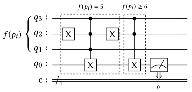
Figure 1 shows an example of post-selection. We use to denote the binary representation of and we use to denote the auxiliary qubit. Assume we have and we are implementing . We add to the last, and then apply the quantum circuit in Figure 1. In the first dashed-line box, we consider the case such that we obtain . In the second dashed-line box, we consider the case such that we obtain . Then, if we measure to be with probability , then we can obtain .
5.1.3. Analysis
Combining amplitude amplification and post-selection, we obtain the algorithm for QQPQθ problems. Motivated by (Boyer et al., 1998), we use the same loop method to solve the problem that is unknown. Algorithm 1 shows the procedure.
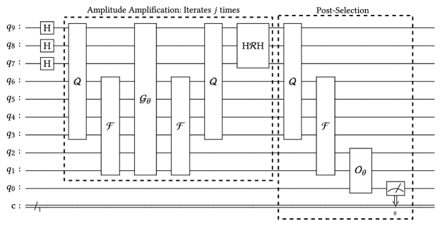
Figure 2 shows an illustration of the quantum circuit. , and store the indices of the tuples. and store the first dimension of the tuple. and store the second dimension of the tuple. and store the utility of the tuple. is the auxiliary qubit in the post-selection. First, we use three Hadamard gates to initialize the indices. After this step, , and all the indices from to . Then, we start to iterate amplitude amplification for times. We first use to read the attributes of the tuples and store the information in and . Then, we use to calculate the utility and store the result in and . After this step, is applied to flip the amplitudes of tuples with utilities larger than . Then, we re-apply and to turn into the initial states so that we can reuse these qubits in the next iterations. The last step in amplitude amplification is to use to amplify the flipped amplitudes. After iterations, we start the post-selection. After applying and in order, we measure . If is , then we obtain the answer in and .
Note that the answer of a QQPQθ problem can be empty, which corresponds to the case that no tuple has utility higher than . If the answer is empty, the algorithm returns as shown in Line 1. Otherwise, it returns the superposition of the desired tuples as shown in Line 1. Such a loop method guarantees that the false negative rate is at most (Boyer et al., 1998), so it can be arbitrarily small if we repeat the process for a constant time. To analyze the complexity, we have the following Theorem 5.1.
Theorem 5.1.
The QQPQθ algorithm needs IOs on average to answer a query.
Proof.
Proved by (Boyer et al., 1998), the expected number of iterations needed is at most . Since each iteration performs QRAM read, the algorithm needs IOs in total. ∎
The complexity shows the advantage of the quantum algorithms, since a larger leads to a lower computational cost, which can never be achieved by any classical algorithms.
5.2. Classical-Output Threshold-Based Quantum Preference Query
Assume there are desired tuples with utilities higher than . In this problem, the algorithm needs to return a list such that is the desired tuples.
We propose the CQPQθ algorithm to solve this problem. Our intuition is that we utilize the superposition returned by QQPQθ algorithm to find the desired tuples in classical bits one by one in a number of iterations. In each -th iteration, the main steps are as follows.
-
•
Step 1: We use QQPQθ algorithm to obtain a superposition of the desired tuples.
-
•
Step 2: We measure the returned qubits. We will obtain a random desired tuple .
-
•
Step 3: We assign a special mark to the -th tuple, such that it will always be assigned the lowest utility by the utility function .
In the -th iteration, there are non-dummy tuples with utilities higher than . We use QQPQθ algorithm to obtain a quantum result . If we measure the result, we randomly obtain one of the desired tuples with probability . Then, we assign to it so that it will not be marked as desired tuples in the subsequent iterations. Algorithm 2 shows the procedure.
To analyze the complexity, we have the following Theorem 5.2.
Theorem 5.2.
The CQPQθ algorithm needs IOs on average to answer a query.
Proof.
By Theorem 5.1, in the -th iteration, QQPQθ algorithm needs IOs since there are desired tuples. Therefore, the total number of IOs needed is
∎
In most real-world cases, we have . Therefore, the complexity has an asymptotically quadratic improvement than classical algorithms that need at least time.
5.3. Classical-Output Top- Quantum Preference Query
In this problem, the algorithm need to return tuples with the highest utilities. The main task is to determine the -th highest utility. We propose the CQPQk algorithm to solve this problem.
In the algorithm, we maintain a min-priority queue. The main steps are as follows.
-
•
Step 1: We randomly pick tuples and insert them into the min-priority queue. We also remove these tuples from the dataset.
-
•
Step 2: We use QQPQθ algorithm to obtain a superposition of tuples among the remaining tuples in the dataset with utilities higher than the minimum utility in the min-priority queue. If is returned, then the min-priority queue exactly contains the desired tuples. Otherwise, we execute Step 3.
-
•
Step 3: We measure the returned qubits which collapse to an resulting tuple, says . We then pop the tuple in the min-priority queue with the minimum utility and push into the queue. We also remove from the dataset. Then, we go back to Step 2.
In each iteration from Step 2 to Step 4, we update the min-priority queue with an tuple with a higher utility. When QQPQθ algorithm returns in Step 2, the min-priority queue cannot be updated any more, so the tuples in the min-priority queue are the desired tuples. Algorithm 3 shows the procedure.
To analyze the complexity, we need to first discuss the probability that each tuple will be inserted into the priority queue. We use to denote the probability that the tuple with the -th highest utility will be inserted into the min-priority queue. Then, the following Lemma 5.3 can be obtained.
Lemma 5.3.
The probability depends on such that
Proof.
If , then the tuple with the -th highest utility must be inserted into , since it is one of the desired tuples. Therefore, .
Then, we discuss the case . If , we have , since we can only insert the tuple in Step 1. Otherwise, the probability contains two parts. The first part is , since each tuple will be inserted into with probability in Step 1. The second part is the probability of insertion in Step 3. We can observe that from the perspective of the tuple with the -th highest utility, each tuple with a higher utility is identical in QQPQθ algorithm, so they will be inserted with the same probability . If , assume it holds for to , then
∎
By Lemma 5.3, we know the probability that each tuple appears in the min-priority queue, which leads to a QQPQθ query and a min-priority queue insertion. To analyze the complexity, we have the following Theorem 5.4.
Theorem 5.4.
The CQPQk algorithm needs IOs on average to answer a query.
Proof.
Since the desired tuples will not trigger another QQPQθ query and a min-priority queue insertion, we only need to calculate the IO cost needed by the other tuples, so we obtain
∎
By Theorem 5.4, the complexity of our proposed CQPQk algorithm is .
5.4. Quantum-Output Top- Quantum Preference Query
In this problem, the algorithm needs to return a superposition of the desired tuples. However, compared to CQPQk problem, there is little hope to obtain further speedup. The reason is that we can only use a classical method as shown in Section 5.3 to determine the -th highest utility, due to the impossibility of comparing quantum states (Arul, 2001). Therefore, to solve QQPQk problem, we propose Algorithm 4 based on QQPQθ algorithm and CQPQk algorithm. Obviously, the complexity of QQPQk algorithm is .
6. Experiment
In this section, we show our experimental results on our quantum preference queries. The study of the real-world quantum supremacy (Arute et al., 2019; Boixo et al., 2018; Terhal, 2018), which is to confirm that a quantum computer can do tasks faster than classical computers, is still a developing topic in the quantum area. We do not aim at verifying quantum supremacy in this paper, but we believe it will be verified in a future quantum computer.
To implement the quantum algorithms and conduct scalability tests, we mainly use C++ to perform the quantum simulations, since existing quantum simulators (e.g., Qiskit (Wille et al., 2019) and Cirq (Gidney C and contributors, 2018)) cannot simulate QRAM effectively. Nevertheless, for a comprehensive comparison, we also implement our algorithms by applying an existing widely-used library (qRAM Library for Q#, 2024) for QRAM simulation (which is implemented with the Q# language) and make comparison with baselines implemented with Q# as well. All algorithms are implemented in a classical machine with 3.6GHz CPU and 32GB memory.
Datasets. We use synthetic and real datasets that were commonly used in existing studies (Borzsony et al., 2001; Tang et al., 2019, 2021). The synthetic datasets include anti-correlated (ANTI), correlated (CORR), independent (INDE) which have different data distributions. The real datasets include HOTEL (Dataset, 2024a), HOUSE (Dataset, 2024b), NBA (Dataset, 2024c). HOTEL includes 419k tuples with 4 attributes (i.e., price and numbers of stars, rooms and facilities). HOUSE includes 315k tuples with 6 attributions (i.e., gas, electricity, water, heating, insurance and property tax). NBA includes 21.9k tuples with 8 attributes (i.e., games, rebounds, assists, steals, blocks, turnovers, personal fouls and points).
Measurement. In this paper, we mainly evaluate the number of memory accesses, which corresponds to the number of IOs in traditional searches. In the quantum algorithms, a QRAM read operation is counted as 1 IO. In the classical algorithms, a page access is counted as 1 IO. IOs cannot be regarded as the real execution time, since we have no any information about the real implementation of a physical QRAM, but they can reflect the potential of the algorithms. Furthermore, we also compare the execution time of algorithms implemented with Q# for additional verification. Note that even with existing QRAM simulation in Q#, the execution time may still be different from that on real quantum computers.
Algorithms. Since there is no classical quantum algorithm returning quantum output, we focused on the classical-output algorithms. We evaluate our algorithms for the top- and threshold-based queries (denoted by QPQk and QPQθ, respectively) with existing classical algorithms Quick Selection (Cormen et al., 2022), -Level Index (Zhang et al., 2022) and Linear Scan. Specifically, we compare QPQk with Quick Selection and -Level Index, and compare QPQθ with Linear Scan (because Quick Selection and -Level Index can only handle the top- queries). Note that -Level Index needs preprocessing which costs up to billions of IOs. However, we do not count the IOs in its preprocessing in comparison and only focused on the IO costs for queries.
Parameter Setting. We evaluated the performance of algorithms by varying several parameters: (1) parameter , used in QPQk; (2) parameter , used in QPQθ; (3) the number of dimensions ; (4) the number of tuples in the dataset ; (5) the category (ANTI, CORR and INDE), which reflects the data distribution in the synthetic datasets. Following (Zhang et al., 2022), K, , by default. For each experimental setting, we randomly generate 100 queries with different utility functions and report the average measurement.
In the following, we show our experimental results.


Results on Top- Preference Queries. We first show the comparison results of top- preference queries (i.e., the CQPQk queries).
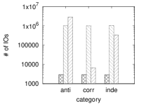
We first study the effect of . In Figure 3, we show the results of dataset ANTI (the representative synthetic dataset) and the three real datasets. As shown in Figure 3(a), for dataset ANTI, our proposed quantum algorithm QPQk has significantly smaller number of IOs than the baselines, which is consistent with the theoretical improvement of our QPQk algorithm. As increases, the IO cost of our QPQk grows more obviously first but very slowly for larger , which verifies the theoretical sub-linear growth of our QPQk to . In comparison, although baseline Quick Selection has similar number of IOs for varied , the number of IOs is very large (i.e., around ) where our QPQk need IO cost of only around for and less than for the largest (i.e., ). Baseline -Level Index also has very large IO cost. Moreover, -Level Index cannot be executed for due to too long preprocessing time, since the preprocessing time increases exponentially with . We obtain similar results on all the three real datasets, as shown in Figure 3(a), (b) and (c).
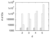
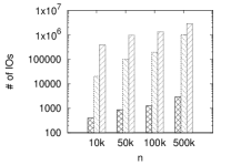
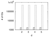
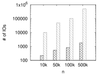
Then, we also study the effect of the number of dimensions , the dataset size and the different categories of synthetic datasets (where the default synthetic dataset if ANTI). As shown in Figure 4(a), has little impact on the IO costs of our QPQk algorithm and Quick Selection, but the IO cost of -Level Index grows significantly with because the geometric processing of hyperplanes depends heavily on . Still, our QPQk has much smaller number of IOs than both baselines. When the dataset size increases (as illustrated in Figure 4(b)), all the algorithms have increased IO cost due to more tuples to be processed. Clearly, our QPQk algorithm has significantly smaller IO cost (due to utilizing the quantum parallelism) compared with both baselines. As shown in Figure 4(c), the IO costs of our QPQk and Quick Selection also do not depend on the dataset category, while -Level Index is more sensitive to dataset category. It indicates that -Level Index could have improvement on certain types of data distribution only, but our QPQk achieves stably superior performance on IO cost.
Results on Threshold-based Preference Queries. Next, we also show the comparison results of threshold-based preference queries (i.e., the CQPQθ queries).
Since the performance is largely affected by the size of the result set (i.e., ), we still vary instead of vary by pick out the -th highest utility from the dataset as the input . As shown in Figure 5, when is varied, the results are very similar as those the CQPQk queries for all the datasets. In particular, the number of IOs of our QPQθ algorithm is no more than 500, or even less than 100 for a relatively smaller dataset (e.g., NBA) which are close to , while the number of IOs of baseline Linear Scan is approximately .
Moreover, when varying , and the dataset category, our QPQθ algorithm also obtains superior results, which are similar to the CQPQk queries. Baseline Linear Scan has much higher IO cost since its IO cost is linear to while our QPQθ achieves quadratic improvement.
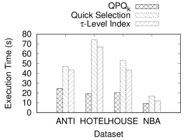
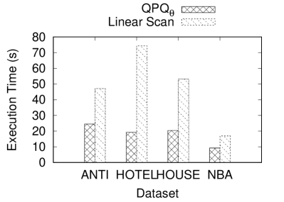
Execution Time Comparison. We also compare the execution time between our algorithms implemented with existing QRAM simulation in Q# and baselines implemented also with Q#.
It can be seen from Figure 7(a) and (b) that, compared with baselines, our proposed quantum algorithms can still achieve superior speed for different datasets, especially those datasets with larger size (e.g., ANTI, HOTEL and HOUSE). However, the execution time improvement (e.g., from 1.3x to 6x) is much smaller than the IO cost improvement (e.g., 1000x). This is because we count each store and load operation of QRAM as 1 IO, but in the existing implementation of QRAM simulators, the time cost cannot be neglected and could be large. Nevertheless, the time improvement of our quantum algorithms could still benefit the real-world applications with the quantum preference queries.
Summary. In conclusion, the quantum algorithm performs far better than the classical algorithms from the perspective of the number of memory accesses. With either input or , our QPQ algorithms are 1000 faster than its classical competitors in typical settings. With the existing QRAM simulators, our proposed quantum algorithms also achieve less execution time than classical baselines. Therefore, we conclude that the quantum algorithms have the potential to outperform classical algorithms.
7. Conclusion
In this paper, we discuss four kinds of QPQ problems: QQPQθ, CQOQθ, CQPQk and QQPQk. We proposed four quantum algorithms to solve these four problems, respectively. For each quantum algorithm, we give an accuracy analysis of the number of memory accesses needed, which shows that the proposed quantum algorithms are at least quadratically faster than their classical competitors. In our experiments, we did simulations to show that to answer a QPQ problem, the quantum algorithms are up to 1000 faster than their classical competitors, which proved that QPQ problem could be a future direction of the study of preference query problems. The future direction of this work is to consider the quantum algorithms for other types of database queries (e.g., the skyline queries).
References
- (1)
- Arul (2001) A John Arul. 2001. Impossibility of comparing and sorting quantum states. arXiv preprint quant-ph/0107085 (2001).
- Arute et al. (2019) Frank Arute, Kunal Arya, Ryan Babbush, Dave Bacon, Joseph C Bardin, Rami Barends, Rupak Biswas, Sergio Boixo, Fernando GSL Brandao, David A Buell, et al. 2019. Quantum supremacy using a programmable superconducting processor. Nature 574, 7779 (2019), 505–510.
- Bayer and McCreight (2002) Rudolf Bayer and Edward McCreight. 2002. Organization and maintenance of large ordered indexes. In Software pioneers. Springer, 245–262.
- Boixo et al. (2018) Sergio Boixo, Sergei V Isakov, Vadim N Smelyanskiy, Ryan Babbush, Nan Ding, Zhang Jiang, Michael J Bremner, John M Martinis, and Hartmut Neven. 2018. Characterizing quantum supremacy in near-term devices. Nature Physics 14, 6 (2018), 595–600.
- Borzsony et al. (2001) Stephan Borzsony, Donald Kossmann, and Konrad Stocker. 2001. The skyline operator. In Proceedings 17th international conference on data engineering. IEEE, 421–430.
- Boyer et al. (1998) Michel Boyer, Gilles Brassard, Peter Høyer, and Alain Tapp. 1998. Tight bounds on quantum searching. Fortschritte der Physik: Progress of Physics 46, 4-5 (1998), 493–505.
- Brassard et al. (2002) Gilles Brassard, Michele Mosca, and Alain Tapp. 2002. Quantum amplitude amplification and estimation. (2002).
- Coppersmith (2002) Don Coppersmith. 2002. An approximate Fourier transform useful in quantum factoring. arXiv preprint quant-ph/0201067 (2002).
- Cormen et al. (2022) Thomas H Cormen, Charles E Leiserson, Ronald L Rivest, and Clifford Stein. 2022. Introduction to algorithms. MIT press.
- Dataset (2024a) Hotel Dataset. 2024a. https://www.hotels-base.com/
- Dataset (2024b) House Dataset. 2024b. https://www.ipums.org/
- Dataset (2024c) NBA Dataset. 2024c. https://www.basketball-reference.com/
- Dirac (1939) Paul Adrien Maurice Dirac. 1939. A new notation for quantum mechanics. In Mathematical Proceedings of the Cambridge Philosophical Society, Vol. 35. Cambridge University Press, 416–418.
- Döring et al. (2008) Sven Döring, Timotheus Preisinger, and Markus Endres. 2008. Advanced preference query processing for e-commerce. In Proceedings of the 2008 ACM symposium on Applied computing. 1457–1462.
- Dürr et al. (2006) Christoph Dürr, Mark Heiligman, Peter HOyer, and Mehdi Mhalla. 2006. Quantum query complexity of some graph problems. SIAM J. Comput. 35, 6 (2006), 1310–1328.
- Durr and Hoyer (1996) Christoph Durr and Peter Hoyer. 1996. A quantum algorithm for finding the minimum. arXiv preprint quant-ph/9607014 (1996).
- Gallego and Wang (2019) Guillermo Gallego and Ruxian Wang. 2019. Threshold utility model with applications to retailing and discrete choice models. Available at SSRN 3420155 (2019).
- Gidney C and contributors (2018) Bacon D Gidney C and contributors. 2018. Cirq: A python framework for creating, editing, and invoking noisy intermediate scale quantum (NISQ) circuits. https://github.com/quantumlib/Cirq.
- Grover (1996a) Lov K Grover. 1996a. A fast quantum mechanical algorithm for database search. In Proceedings of the twenty-eighth annual ACM symposium on Theory of computing. 212–219.
- Grover (1996b) Lov K Grover. 1996b. A fast quantum mechanical algorithm for estimating the median. arXiv preprint quant-ph/9607024 (1996).
- Grover and Radhakrishnan (2005) Lov K Grover and Jaikumar Radhakrishnan. 2005. Is partial quantum search of a database any easier?. In Proceedings of the seventeenth annual ACM symposium on Parallelism in algorithms and architectures. 186–194.
- Hadamard (1893) Jacques Hadamard. 1893. Resolution d’une question relative aux determinants. Bull. des sciences math. 2 (1893), 240–246.
- Harrow et al. (2009) Aram W Harrow, Avinatan Hassidim, and Seth Lloyd. 2009. Quantum algorithm for linear systems of equations. Physical review letters 103, 15 (2009), 150502.
- Hosoyamada and Sasaki (2018) Akinori Hosoyamada and Yu Sasaki. 2018. Quantum Demiric-Selçuk meet-in-the-middle attacks: applications to 6-round generic Feistel constructions. In International Conference on Security and Cryptography for Networks. Springer, 386–403.
- Jerbi et al. (2021) Sofiene Jerbi, Casper Gyurik, Simon Marshall, Hans Briegel, and Vedran Dunjko. 2021. Parametrized Quantum Policies for Reinforcement Learning. Advances in Neural Information Processing Systems 34 (2021).
- Kapoor et al. (2016) Ashish Kapoor, Nathan Wiebe, and Krysta Svore. 2016. Quantum perceptron models. Advances in neural information processing systems 29 (2016).
- Kapralov et al. (2020) Ruslan Kapralov, Kamil Khadiev, Joshua Mokut, Yixin Shen, and Maxim Yagafarov. 2020. Fast Classical and Quantum Algorithms for Online -server Problem on Trees. arXiv preprint arXiv:2008.00270 (2020).
- Kerenidis et al. (2019) Iordanis Kerenidis, Jonas Landman, Alessandro Luongo, and Anupam Prakash. 2019. q-means: A quantum algorithm for unsupervised machine learning. Advances in Neural Information Processing Systems 32 (2019).
- Kerenidis and Prakash (2017) Iordanis Kerenidis and Anupam Prakash. 2017. Quantum Recommendation Systems. In 8th Innovations in Theoretical Computer Science Conference (ITCS 2017). Schloss Dagstuhl-Leibniz-Zentrum fuer Informatik.
- Kieferova et al. (2021) Maria Kieferova, Ortiz Marrero Carlos, and Nathan Wiebe. 2021. Quantum Generative Training Using R’enyi Divergences. arXiv preprint arXiv:2106.09567 (2021).
- Lee et al. (2009) Jongwuk Lee, Gae-won You, and Seung-won Hwang. 2009. Personalized top-k skyline queries in high-dimensional space. Information Systems 34, 1 (2009), 45–61.
- Li et al. (2021b) Guangxi Li, Zhixin Song, and Xin Wang. 2021b. VSQL: variational shadow quantum learning for classification. In Proceedings of the AAAI Conference on Artificial Intelligence, Vol. 35. 8357–8365.
- Li et al. (2021a) Qiuchi Li, Dimitris Gkoumas, Alessandro Sordoni, Jian-Yun Nie, and Massimo Melucci. 2021a. Quantum-inspired neural network for conversational emotion recognition. In Proceedings of the AAAI Conference on Artificial Intelligence, Vol. 35. 13270–13278.
- Li et al. (2019) Tongyang Li, Shouvanik Chakrabarti, and Xiaodi Wu. 2019. Sublinear quantum algorithms for training linear and kernel-based classifiers. In International Conference on Machine Learning. PMLR, 3815–3824.
- Li et al. (2021c) Tongyang Li, Chunhao Wang, Shouvanik Chakrabarti, and Xiaodi Wu. 2021c. Sublinear Classical and Quantum Algorithms for General Matrix Games. In Proceedings of the AAAI Conference on Artificial Intelligence, Vol. 35. 8465–8473.
- Lian and Chen (2009) Xiang Lian and Lei Chen. 2009. Top-k dominating queries in uncertain databases. In Proceedings of the 12th international conference on extending database technology: advances in database technology. 660–671.
- Liang et al. (2011) Shenshen Liang, Ying Liu, Liheng Jian, Yang Gao, and Zhu Lin. 2011. A utility-based recommendation approach for academic literatures. In 2011 IEEE/WIC/ACM International Conferences on Web Intelligence and Intelligent Agent Technology, Vol. 3. IEEE, 229–232.
- Miao et al. (2016) Xiaoye Miao, Yunjun Gao, Gang Chen, Huiyong Cui, Chong Guo, and Weida Pan. 2016. SI2P: A restaurant recommendation system using preference queries over incomplete information. Proceedings of the VLDB Endowment 9, 13 (2016), 1509–1512.
- Montanaro (2017) Ashley Montanaro. 2017. Quantum pattern matching fast on average. Algorithmica 77, 1 (2017), 16–39.
- Naya-Plasencia and Schrottenloher (2020) María Naya-Plasencia and André Schrottenloher. 2020. Optimal Merging in Quantum -xor and -sum Algorithms. In Annual International Conference on the Theory and Applications of Cryptographic Techniques. Springer, 311–340.
- Nielsen and Chuang (2001) Michael A Nielsen and Isaac L Chuang. 2001. Quantum computation and quantum information. Phys. Today 54, 2 (2001), 60.
- Peng and Wong (2015) Peng Peng and Raymong Chi-Wing Wong. 2015. k-hit query: Top-k query with probabilistic utility function. In Proceedings of the 2015 ACM SIGMOD International Conference on Management of Data. 577–592.
- Pivert and Bosc (2012) Olivier Pivert and Patrick Bosc. 2012. Fuzzy preference queries to relational databases. World Scientific.
- qRAM Library for Q# (2024) qRAM Library for Q#. 2024. https://github.com/qsharp-community/qram
- Rebentrost et al. (2014) Patrick Rebentrost, Masoud Mohseni, and Seth Lloyd. 2014. Quantum support vector machine for big data classification. Physical review letters 113, 13 (2014), 130503.
- Regenwetter et al. (1998) Michel Regenwetter, AAJ Marley, and H Joe. 1998. Random utility threshold models of subset choice. Australian Journal of Psychology 50, 3 (1998), 175–185.
- Rocha-Junior et al. (2010) Joao B Rocha-Junior, Akrivi Vlachou, Christos Doulkeridis, and Kjetil Nørvåg. 2010. Efficient processing of top-k spatial preference queries. Proceedings of the VLDB Endowment 4, 2 (2010), 93–104.
- Saeedi and Arodz (2019) Seyran Saeedi and Tom Arodz. 2019. Quantum sparse support vector machines. arXiv preprint arXiv:1902.01879 (2019).
- Schenkel et al. (2008) Ralf Schenkel, Tom Crecelius, Mouna Kacimi, Sebastian Michel, Thomas Neumann, Josiane X Parreira, and Gerhard Weikum. 2008. Efficient top-k querying over social-tagging networks. In Proceedings of the 31st annual international ACM SIGIR conference on Research and development in information retrieval. 523–530.
- Schrödinger (1935) Erwin Schrödinger. 1935. Discussion of probability relations between separated systems. In Mathematical Proceedings of the Cambridge Philosophical Society, Vol. 31. Cambridge University Press, 555–563.
- Seidel et al. (2021) Raphael Seidel, Colin Kai-Uwe Becker, Sebastian Bock, Nikolay Tcholtchev, Ilie-Daniel Gheorge-Pop, and Manfred Hauswirth. 2021. Automatic Generation of Grover Quantum Oracles for Arbitrary Data Structures. arXiv preprint arXiv:2110.07545 (2021).
- Shor (1994) Peter W Shor. 1994. Algorithms for quantum computation: discrete logarithms and factoring. In Proceedings 35th annual symposium on foundations of computer science. Ieee, 124–134.
- Soliman and Ilyas (2009) Mohamed A. Soliman and Ihab F. Ilyas. 2009. Ranking with uncertain scores. In Proceedings of the International Conference on Data Engineering. 317–328.
- Tang et al. (2021) Bo Tang, Kyriakos Mouratidis, and Mingji Han. 2021. On m-impact regions and standing top-k influence problems. In Proceedings of the 2021 International Conference on Management of Data. 1784–1796.
- Tang et al. (2019) Bo Tang, Kyriakos Mouratidis, Man Lung Yiu, and Zhenyu Chen. 2019. Creating top ranking options in the continuous option and preference space. (2019).
- Terhal (2018) Barbara M Terhal. 2018. Quantum supremacy, here we come. Nature Physics 14, 6 (2018), 530–531.
- Toffoli (1980) Tommaso Toffoli. 1980. Reversible computing. In International colloquium on automata, languages, and programming. Springer, 632–644.
- Wang et al. (2017) Yan Wang, Zhan Shi, Junlu Wang, Lingfeng Sun, and Baoyan Song. 2017. Skyline preference query based on massive and incomplete dataset. IEEE Access 5 (2017), 3183–3192.
- Wiebe et al. (2012) Nathan Wiebe, Daniel Braun, and Seth Lloyd. 2012. Quantum algorithm for data fitting. Physical review letters 109, 5 (2012), 050505.
- Wiebe et al. (2015) Nathan Wiebe, Ashish Kapoor, and Krysta M Svore. 2015. Quantum algorithms for nearest-neighbor methods for supervised and unsupervised learning. Quantum Information & Computation 15, 3-4 (2015), 316–356.
- Wille et al. (2019) Robert Wille, Rod Van Meter, and Yehuda Naveh. 2019. IBM’s Qiskit tool chain: Working with and developing for real quantum computers. In 2019 Design, Automation & Test in Europe Conference & Exhibition (DATE). IEEE, 1234–1240.
- Yiu et al. (2007) Man Lung Yiu, Xiangyuan Dai, Nikos Mamoulis, and Michail Vaitis. 2007. Top-k spatial preference queries. In 2007 IEEE 23rd International Conference on Data Engineering. IEEE, 1076–1085.
- Zhang et al. (2022) Jiahao Zhang, Bo Tang, Man Lung Yiu, Xiao Yan, and Keming Li. 2022. T-LevelIndex: Towards Efficient Query Processing in Continuous Preference Space. In Proceedings of the 2022 International Conference on Management of Data. 2149–2162.
- Zhang and Korepin (2018) Kun Zhang and Vladimir Korepin. 2018. Quantum partial search for uneven distribution of multiple target items. Quantum Information Processing 17, 6 (2018), 1–20.