A Bayesian joint model of multiple nonlinear longitudinal and competing risks outcomes for dynamic prediction in multiple myeloma: joint estimation and corrected two-stage approaches

Abstract

Predicting cancer-associated clinical events is challenging in oncology. In Multiple Myeloma (MM), a cancer of plasma cells, disease progression is determined by changes in biomarkers, such as serum concentration of the paraprotein secreted by plasma cells (M-protein). Therefore, the time-dependent behaviour of M-protein and the transition across lines of therapy (LoT) that may be a consequence of disease progression should be accounted for in statistical models to predict relevant clinical outcomes. Furthermore, it is important to understand the contribution of the patterns of longitudinal biomarkers, upon each LoT initiation, to time-to-death or time-to-next-LoT. Motivated by these challenges, we propose a Bayesian joint model for trajectories of multiple longitudinal biomarkers, such as M-protein, and the competing risks of death and transition to next LoT. Additionally, we explore two estimation approaches for our joint model: simultaneous estimation of all parameters (joint estimation) and sequential estimation of parameters using a corrected two-stage strategy aiming to reduce computational time. Our proposed model and estimation methods are applied to a retrospective cohort study from a real-world database of patients diagnosed with MM in the US from January 2015 to February 2022. We split the data into training and test sets in order to validate the joint model using both estimation approaches and make dynamic predictions of times until clinical events of interest, informed by longitudinally measured biomarkers and baseline variables available up to the time of prediction.
Keywords: Bayesian inference; Bi-exponential model; Cause-specific hazards; Free light chains; M-spike.

1 Introduction

Recent trends in personalised healthcare have motivated great interest in the individual dynamic risk prediction of survival and other clinically important events by using baseline characteristics and the course of disease progression (Barrett and Su, 2017; Ferrer et al., 2019; Ren et al., 2021; Parr et al., 2022). In particular, studies of Multiple Myeloma (MM, the second most common hematological cancer) have identified several risk factors that may help to predict the disease course (Abdallah et al., 2023; Zhang et al., 2023). In this type of blood cancer, malignant plasma cells accumulate in the bone marrow and secrete a monoclonal protein/paraprotein (also known as M-protein). The time-dependent assessment of M-protein concentration through serum protein electrophoresis (SPEP/M-spike) and/or involved free light chains (FLC), e.g. through FreeLite${}^{\text{\scriptsize\textregistered}}$ test, may provide useful information to the treating physician about the individual risk of a patient to experience either one of two clinical events of interest: death or start of a new line of therapy (LoT) (Kumar et al., 2017).

To understand the dynamic interplay between longitudinal biomarkers and their associations with clinical outcomes, we propose a new Bayesian joint model that appropriately accommodates different characteristics of MM data. Specifically, upon each LoT initiation, the temporal profiles of M-spike and FLC are nonlinear, and could adequately be characterised by a bi-exponential model (Stein et al., 2008). This model presents three components (baseline, growth rate, decay rate parameters) to summarise the longitudinal trajectory and to explain the time until clinical events of interest (death or start of next LoT). These two clinical events are modelled as competing risks, in which we use a proportional cause-specific hazard specification (Putter et al., 2020).

The simultaneous estimation of all parameters in a joint model is computationally intensive due to the complexity of approximating posterior distributions from multiple nonlinear longitudinal submodels sharing information with a competing risks submodel (Hickey et al., 2016; Mauff et al., 2020). As an alternative approach, we explore the corrected two-stage approach proposed by Alvares and Leiva-Yamaguchi (2023). This approach reduces computational complexity by estimating the submodels separately and produces results similar to those of simultaneous estimation due to a bias correction mechanism incorporated in the second stage. Previous works have shown such inferential similarity between both approaches (Alvares and Leiva-Yamaguchi, 2023; Alvares and Mercier, 2024), but it is unclear whether they also produce similar predictions. Thus, we also intend to shed light on this topic through comparisons using predictive metrics and individual dynamic predictions. Hence, a corrected two-stage proposal is compared to the joint estimation approach using a retrospective cohort study of patients diagnosed with MM and who received at least one LoT between January 2015 and February 2022.

The rest of the work is organised as follows. Section 2 describes a multiple myeloma retrospective cohort study from the US nationwide Flatiron Health database. Driven by such data, Section 3 presents a Bayesian joint model of multiple nonlinear longitudinal and competing risks outcomes. Section 4 introduces the joint estimation and corrected two-stage approaches, model performance evaluation criteria, and a dynamic risk prediction scheme. Section 5 compares both estimation approaches applied to multiple myeloma data. The work ends with a discussion in Section 6.

2 Multiple Myeloma Data

Personalised patient management in diseases like MM is currently challenging due to disease heterogeneity and shortcomings of existing models to accurately predict patients at high risk of clinical events of interest, e.g. early relapse in MM (van de Velde et al., 2007; Lahuerta et al., 2008; Martínez-López et al., 2011; Rees and Kumar, 2024). Motivated by this context, we leveraged de-identified patient-level data from Flatiron Health electronic health record (EHR)-derived database of patients diagnosed with MM in the US. The Flatiron Health database is a nationwide longitudinal, demographically, and geographically diverse database derived from EHR data (Ma et al., 2023). In totality, it includes de-identified data from over 280 cancer clinics (approximately 800 sites of care), representing more than 2.4 million patients with active cancer in the US (Kumar et al., 2021). The majority of patients in the database originate from community oncology settings; relative community/academic proportions may vary depending on study cohort. The patient-level data in EHRs includes structured data (e.g. laboratory values and prescribed drugs) in addition to unstructured data collected via technology-enabled chart abstraction from physician’s notes and other documents (e.g. biomarker reports and discharge summaries) (Birnbaum et al., 2020).

For our analyses, the follow-up period is defined from 1st January 2015 to 28th February 2022. Patients included in the database were diagnosed with MM on or after 1st January 2015 and presented at least two visits in the Flatiron Health system. Other eligibility criteria are: (i) at least 18 years of age at MM diagnosis, (ii) no longer than 60 days between initial diagnosis and first activity (visit or LoT initiation), (iii) more than three months on-treatment before the end of study follow-up, (iv) and no malignancies before MM diagnosis. Thus, 5490 patients formed the sample of newly diagnosed MM patients who met all eligibility criteria. Table 1 shows the number of patients who died, transitioned to next LoT, or were censored (neither experienced death nor started next LoT) and their respective median time until the event within each LoT (LoT in the database was oncologist-defined, rule-based). For example, of the 5490 patients who started LoT 1, 843 (15%) died during LoT 1, 2775 (51%) changed to LoT 2, 1872 (34%) were censored during LoT 1, and their respective median time on LoT 1 was 210, 266, and 198 days. Note that we grouped LoT 5 and beyond, into LoT 4 due to the small number of patients (e.g. 362 in LoT 5). In practice, this means that from LoT 4 onwards, only death or censoring can occur.

Table 1: Number of cases, percentages, and median times (in days) of patients who died, transitioned to next line of therapy (LoT), and were censored within each LoT $l=1,2,3,4$.

LoT	Death		LoT $\bm{l+1}$		Censored		Total
	Cases (%)	Median	Cases (%)	Median	Cases (%)	Median
$l=1$	843 (15)	210	2775 (51)	266	1872 (34)	198	5490
$l=2$	400 (14)	189	1401 (51)	226	974 (35)	292	2775
$l=3$	246 (18)	127	716 (51)	174	439 (31)	290	1401
$l=4$	290 (41)	268			426 (59)	455	716

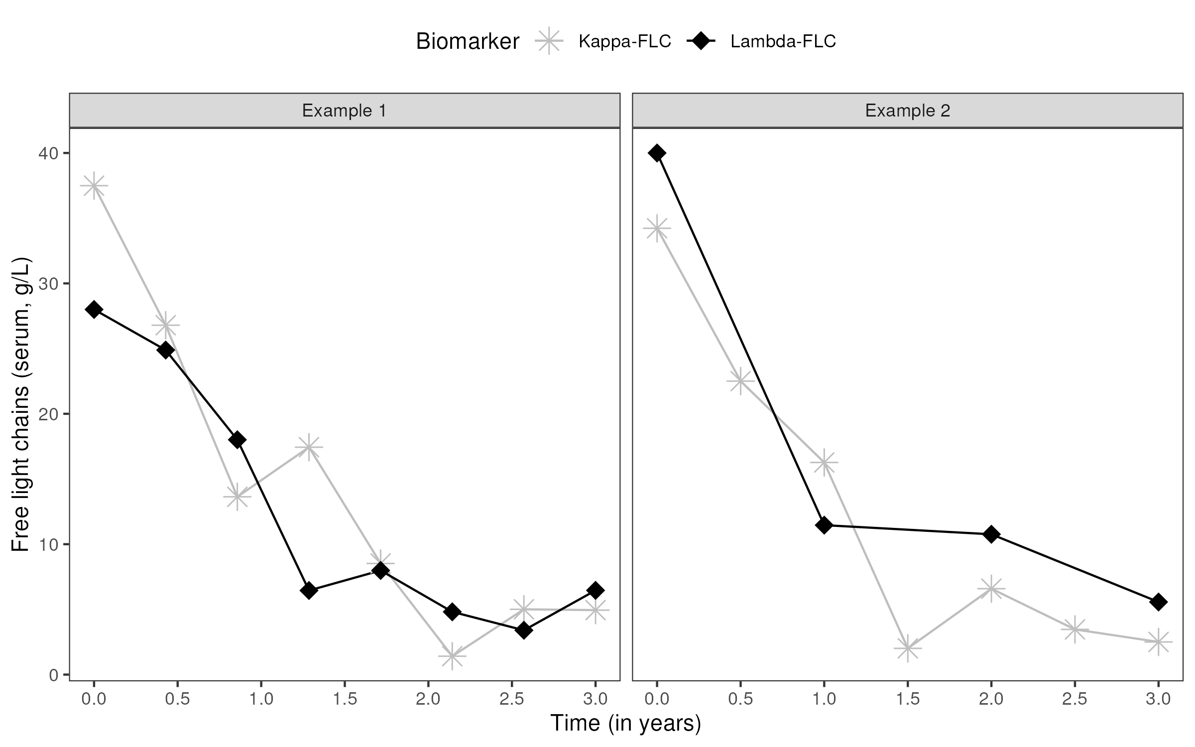
Figure 1: Illustrations of kappa and lambda free light chain (FLC) trajectories. In Example 1 (left), as the first kappa-FLC value is higher than the first lambda-FLC value, only kappa-FLC values are followed through. In Example 2 (right) the opposite occurs, as the first lambda-FLC value is higher than the first kappa-FLC value, only lambda-FLC values are followed through.

In addition to times until clinical events of interest, the Flatiron Health database also provides observations for the longitudinal biomarkers that predict the probability of the clinical event of interest occurring. Here we use SPEP/M-spike results to quantify the concentration of M-protein in serum (g/L) and FLC to quantify the concentration of involved light chains (either kappa or lambda, g/L). Due to varying clinical guidelines and practices, a large number of patients may not always have both of these biomarkers or even different recording frequencies. Hence, for patients with both kappa-FLC and lambda-FLC, the chain of the higher initial value is followed through (see examples in Web Figure 1). Web Table 1 shows a summary of the distribution of the number of M-spike and FLC measurements per patient by LoT.

Baseline characteristics collected at initial diagnosis are available for the categorical variables: sex, ethnicity, Eastern Cooperative Oncology Group (ECOG), and International Staging System (ISS) (see a descriptive summary in Web Table 2), as well as for the continuous variables: age, albumin (serum, g/L), beta-2-microglobulin (B2M, serum, mg/L), creatinine (serum, mg/dL), hemoglobin (g/dL), lactate dehydrogenase (LDH, serum, U/L), lymphocyte (count, $\times 10^{9}$/L), neutrophil (count, $\times 10^{9}$/L), platelet (count, $\times 10^{9}$/L), immunoglobulin A (IgA, serum, g/L), IgG (serum, g/L), IgM (serum, g/L) (see a descriptive summary in Web Table 3). From LoT 2 onwards, we can use the time spent in the previous LoT as an explanatory variable. Except for age and time spent in the previous LoT, all continuous variables have missing data. To handle such variables, we apply a log transformation to reduce asymmetry, a standardisation so that their scales are similar, and a simple imputation to fill in missing observations (see Web Table 3).

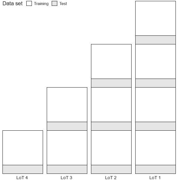
Figure 2: Data splitting scheme into training and test sets by line of therapy (LoT). From bottom to top, first row represents patients in LoTs 1-4, and last one represents patients in LoT 1 but not in LoTs 2-4.

For each LoT, we randomly select 80% of the data to be the training set (used to fit, calibrate, and validate the model) and the remaining 20% comprise the test set (a hold-out dataset to evaluate the model performance and make predictions). Web Figure 2 illustrates our train-test split strategy by LoT.

3 The Bayesian Joint Model

A joint model of longitudinal and survival outcomes was developed to account for the complexity of the data and research questions (Rizopoulos, 2012). Specifically, biomarkers are endogenous time-varying covariates, where their trajectories can be modelled through a suitable longitudinal submodel; time-to-death and time-to-next-LoT can be modelled with a competing risks submodel, where individual-level information is allowed to be shared across submodels. In addition, we considered a Bayesian approach due to the ease of incorporating it into hierarchical structures, quantifying uncertainty, and making dynamic predictions as new observations become available (Desmée et al., 2017a; Alsefri et al., 2020; Kerioui et al., 2020). Moreover, we adopted a blockwise inferential scheme to reduce the complexity of a multistate framework (Chen et al., 2023). Figure 1 illustrates this strategy. Note that each LoT has its own joint model and each of these is independent of the others. This reduces the number of parameters to be estimated simultaneously and provides the possibility of running joint models in parallel. It is also worth highlighting that this strategy naturally considers a clock-reset specification (Kleinbaum and Klein, 2012) at the start of each LoT.

Figure 1: Graphical representation of joint modelling for MM data based on a blockwise inferential scheme. Circle: longitudinal submodel. Rectangle: time-to-event submodel. M: M-spike, F: free light chains. LoT: line of therapy.

We describe in the following the step-by-step construction of our Bayesian joint model: its submodels and the setting for priors.

3.1 Longitudinal Submodels

We specify the longitudinal processes that model M-spike ($k=1$) and free light chains ($k=2$) biomarkers through a bi-exponential model (Stein et al., 2008). Mathematically, such a model is given by

$$y_{kli}(t)=B_{kli}\Big{[}\exp\left\{G_{kli}t\right\}+\exp\left\{-D_{kli}t\right\}-1\Big{]}+\epsilon_{kli}(t),$$ (1)

where $y_{kli}(t)$ represents the observed value of biomarker $k=1,2$ in line of therapy (LoT) $l=1,2,3,4$ for patient $i=1,\ldots,n_{l}$ at time $t$ ($t=0$ indicates the therapy start time). $B_{kli}$, $G_{kli}$, and $D_{kli}$ are parameters that take only positive values and represent baseline (the biomarker value at $t=0$), growth rate, and decay rate, respectively, which are characteristics associated with the biomarker’s longitudinal trajectory. The residual errors, $\epsilon_{kl1}(t),\ldots,\epsilon_{kln_{l}}(t)$, are assumed additive, independent and identically distributed as $\epsilon_{kli}(t)\sim\mbox{Normal}(0,\sigma_{kl}^{2})$.

We redefine the three parameters of the (1) as $B_{kli}=\exp\left\{\theta_{1kl}+b_{kli1}\right\}$, $G_{kli}=\exp\left\{\theta_{2kl}+b_{kli2}\right\}$, and $D_{kli}=\exp\left\{\theta_{3kl}+b_{kli3}\right\}$, where ${\bm{\theta}}_{kl}=(\theta_{1kl},\theta_{2kl},\theta_{3kl})^{\top}$ are population parameters while ${\bm{b}}_{kli}=(b_{kli1},b_{kli2},b_{kli3})^{\top}$ are random effects. In addition, we assume that ${\bm{b}}_{kli}\sim\mbox{Normal}({\bm{0}},{\bm{\Omega}}_{kl})$, where ${\bm{\Omega}}_{kl}$ is an unstructured variance-covariance matrix.

Note that we opted to specify two univariate bi-exponential models (i.e., $k=1$ and $k=2$ in (1) are independent of each other) instead of a bivariate one. This simplification was made to overcome convergence issues introduced by having many random effects per LoT ($2\times 3\times n_{l}$) and non-linearity.

3.2 Competing Risks Submodels

We model time-to-death ($v=1$) and time-to-next-LoT ($v=2$) through a competing risks model (Putter et al., 2007), via a proportional cause-specific hazard specification (Putter et al., 2020). We denote $T_{lvi}$ as the time from the start of LoT $l$ to the occurrence of event $v$ for patient $i$; $C_{li}$ indicates the censoring time for patient $i$ in LoT $l$; $\delta_{li}=0,1,2$ is an event indicator, where $\delta_{li}=0$ represents censoring for both events in LoT $l$, $\delta_{li}=1$ indicates that patient $i$ died in LoT $l$, and $\delta_{li}=2$ that patient $i$ transitioned to LoT $l+1$; and $T_{li}=\min\{T_{l1i},T_{l2i},C_{li}\}$ represents the observed event time for patient $i$ in LoT $l$. For a LoT $l$, we specify the hazard function of patient $i$ for event $v$ at time $t$ given by

$$h_{lvi}(t)=h_{lv0}(t)\exp\left\{{\bm{X}}_{lvi}^{\top}{\bm{\beta}}_{lv}+\sum_{k=1}^{2}\big{(}\alpha_{klv1}B_{kli}^{\ast}+\alpha_{klv2}G_{kli}^{\ast}+\alpha_{klv3}D_{kli}^{\ast}\big{)}\right\},$$ (2)

where $h_{lv0}(t)$ represents a baseline hazard function and is defined throughout this work as a Weibull hazard given by $h_{lv0}(t)=\phi_{lv}t^{\phi_{lv}-1}\exp\{\beta_{lv0}\}$, where $\phi_{lv}$ and $\beta_{lv0}$ are shape and log-scale parameters; ${\bm{X}}_{lvi}$ is a covariate vector with coefficients ${\bm{\beta}}_{lv}$; $B_{kli}^{\ast}=\log(B_{kli})$, $G_{kli}^{\ast}=\log(G_{kli})$, and $D_{kli}^{\ast}=\log(D_{kli})$ are the baseline, growth rate, and decay rate (in log scale) of biomarker $k$ in LoT $l$ for patient $i$, shared from the longitudinal submodel (1), where $\alpha_{klv1}$, $\alpha_{klv2}$, and $\alpha_{klv3}$ have the role of measuring the strength of association between each characteristic of the biomarker trajectory and the risk for event $v$. As we adopted a cause-specific competing risks specification, the overall survival function of (2) for $v=1,2$ is defined as $S_{li}(t)=\exp\{-H_{l1i}(t)-H_{l2i}(t)\}$, where $H_{lvi}(t)$ is the cumulative hazard of $h_{lvi}(t)$. Note that for LoT $l=4$ we do not have a competing risks specification (see Figure 1) but instead a proportional hazard model for time-to-death ($v=1$ only).

In preliminary analyses, we evaluated different parametric baseline hazard functions (exponential and Gompertz) and different shared terms (current value, only one of the parameters $B_{kli}^{\ast}$, $G_{kli}^{\ast}$, and $D_{kli}^{\ast}$, or pairs thereof), including dependence on previous LoT parameters, $B_{k(l-1)i}^{\ast}$, $G_{k(l-1)i}^{\ast}$, and $D_{k(l-1)i}^{\ast}$, which were not significant. The best specification was the one used in (2) (without previous LoT summaries) according to the leave-one-out cross-validation (LOO-CV) and the widely applicable information criterion (WAIC) (Vehtari et al., 2017).

3.3 Prior Elicitation

We assume independent and weakly informative marginal prior distributions (Gelman et al., 2013). For each biomarker $k=1,2$ and LoT $l=1,2,3,4$ using the longitudinal submodel (1), the population parameters $\theta_{1kl}$, $\theta_{2kl}$, and $\theta_{3kl}$ follow Normal($0,10^{2}$) prior distributions, the residual error variance, $\sigma_{kl}^{2}$, follows a half-Cauchy($0,5$) prior distribution (Gelman, 2006), and the random effects variance-covariance matrix ${\bm{\Omega}}_{kl}$ follows an inverse-Wishart($\mathbf{I}_{3},4$) prior distribution (Schuurman et al., 2016), where $\mathbf{I}_{3}$ represents a $3\times 3$ identity matrix. For each LoT $l=1,2,3,4$ and competing risk events $v=1,2$ using the survival submodel (2), the regression coefficients ${\bm{\beta}}_{lv}$ (including the Weibull log-scale $\beta_{lv0}$) and the association parameters $\alpha_{klv1}$, $\alpha_{klv2}$, and $\alpha_{klv3}$ follow Normal($0,10^{2}$) prior distributions, and the Weibull shape parameter, $\phi_{lv}$, follows a half-Cauchy($0,1$) prior distribution (Rubio and Steel, 2018).

4 Posterior Inference and Prediction

4.1 Joint Estimation (JE) Approach

For each LoT $l=1,2,3,4$, we assume that longitudinal processes ${\bm{y}}_{1l}$ and ${\bm{y}}_{2l}$ are independent of each other and that they are conditionally independent of competing risk process ${\bm{s}}_{l}$ given the shared information $({\bm{\theta}}_{1l},{\bm{\theta}}_{2l},{\bm{b}}_{1l},{\bm{b}}_{2l})$, where ${\bm{b}}_{kl}=({\bm{b}}_{kl1},\ldots,{\bm{b}}_{kln_{l}})$ is the vector of all individual-level random effects of biomarker $k$ in LoT $l$. So, for a LoT $l$, the joint posterior distribution of all parameters is proportionally expressed as follows:

$$\pi({\bm{\theta}}_{1l},{\bm{\theta}}_{2l},{\bm{\Psi}}_{1l},{\bm{\Psi}}_{2l},{\bm{\Phi}}_{l},{\bm{b}}_{1l},{\bm{b}}_{2l}\mid{\mathcal{D}}_{l}) \propto f_{1}({\bm{y}}_{1l}\mid{\bm{\theta}}_{1l},{\bm{b}}_{1l},{\bm{\Psi}}_{1l})f_{2}({\bm{y}}_{2l}\mid{\bm{\theta}}_{2l},{\bm{b}}_{2l},{\bm{\Psi}}_{2l})\times$$ (3)

$$\times f_{3}({\bm{s}}_{l}\mid{\bm{\theta}}_{1l},{\bm{\theta}}_{2l},{\bm{b}}_{1l},{\bm{b}}_{2l},{\bm{\Phi}}_{l})g_{1}({\bm{b}}_{1l}\mid{\bm{\Psi}}_{1l})g_{2}({\bm{b}}_{2l}\mid{\bm{\Psi}}_{2l})\pi({\bm{\theta}}_{1l},{\bm{\theta}}_{2l},{\bm{\Psi}}_{1l},{\bm{\Psi}}_{2l},{\bm{\Phi}}_{l}),$$

where ${\mathcal{D}}_{l}=\{{\bm{y}}_{1li},{\bm{y}}_{2li},T_{li},\delta_{li},{\bm{X}}_{l\cdot i};\,i=1,\ldots,n_{l}\}$ denotes data available (training set) for LoT $l$; ${\bm{\Psi}}_{1l}=({\bm{\Omega}}_{1l},\sigma_{1l}^{2})$, ${\bm{\Psi}}_{2l}=({\bm{\Omega}}_{2l},\sigma_{2l}^{2})$, and ${\bm{\Phi}}_{l}=({\bm{\beta}}_{l},{\bm{\alpha}}_{1l},{\bm{\alpha}}_{2l},{\bm{\phi}}_{l})$; the density functions $f_{1}(\cdot)$, $f_{2}(\cdot)$, and $f_{3}(\cdot)$, derived from the longitudinal submodel (1) for biomarkers $k=1,2$ and the competing risks submodel (2), are expressed as follows:

$$f_{k}({\bm{y}}_{kl}\mid\cdot) =\prod_{i=1}^{n_{l}}\prod_{j=1}^{m_{kli}}\frac{1}{\sqrt{2\pi\sigma_{kl}^{2}}}\exp\left\{-\frac{1}{\sigma_{kl}^{2}}\big{(}y_{kli}(t_{klij})-\mu_{kli}(t_{klij})\big{)}^{2}\right\},\text{ for }k=1,2,$$ (4)

$$f_{3}({\bm{s}}_{l}\mid\cdot) =\prod_{i=1}^{n_{l}}h_{l1i}(T_{li})^{1_{(\delta_{li}=1)}}\,h_{l2i}(T_{li})^{1_{(\delta_{li}=2)}}\exp\left\{-\int_{0}^{T_{li}}\big{[}h_{l1i}(t)+h_{l2i}(t)\big{]}\text{d}t\right\},$$ (5)

where $\mu_{kli}(t)=B_{kli}\big{[}\exp\left\{G_{kli}t\right\}+\exp\left\{-D_{kli}t\right\}-1\big{]}$ is the true and unobserved trajectory of biomarker $k=1,2$ evaluated at time $t$, and $t_{klij}=1,\ldots,m_{kli}$ represent the time points at which biomarker values ($k=1,2$) are recorded in LoT $l$ for patient $i$; $g_{1}(\cdot)$ and $g_{2}(\cdot)$ are Normal densities for random effects ${\bm{b}}_{1l}$ and ${\bm{b}}_{2l}$, respectively; and $\pi(\cdot)$ is the prior distribution specified as in Section 3.3.

4.2 Corrected Two-Stage (TS) Approach

Typically, calculating posterior distributions from joint models, such as in (3), is computationally demanding and their complexity may also cause convergence problems (Mehdizadeh et al., 2021). Both issues are avoided using a standard two-stage estimation, where the longitudinal submodel is first fitted, shared quantities are estimated and, in a second stage, inserted as known covariates into the survival submodel. However, several studies have shown that this strategy leads to biased results (Tsiatis and Davidian, 2004; Ye et al., 2008; Sweeting and Thompson, 2011; Hickey et al., 2016; Leiva-Yamaguchi and Alvares, 2021). Recently, Alvares and Leiva-Yamaguchi (2023) proposed a corrected two-stage approach that mitigates such estimation biases. The authors developed this methodology in the context of exponential family distributions with linear predictors for a longitudinal outcome and a proportional hazard model. Alvares and Mercier (2024) also used a univariate time-to-event outcome but extrapolated the original proposal to a bi-exponential model (i.e., a nonlinear predictor) with a multiplicative error term. Here we extend this corrected two-stage approach to multiple bi-exponential models and competing risks survival outcomes. More specifically, in the first stage, we calculate the maximum a posteriori of the parameters of each longitudinal submodel in LoT $l$:

$$(\hat{\bm{\theta}}_{1l},\hat{\bm{\Psi}}_{1l}) =\operatorname*{arg\,max}_{{\bm{\theta}}_{1l},\,{\bm{\Psi}}_{1l}}f_{1}({\bm{y}}_{1l}\mid{\bm{\theta}}_{1l},{\bm{b}}_{1l},{\bm{\Psi}}_{1l})g_{1}({\bm{b}}_{1l}\mid{\bm{\Psi}}_{1l})\pi({\bm{\theta}}_{1l},{\bm{\Psi}}_{1l}),$$ (6)

$$(\hat{\bm{\theta}}_{2l},\hat{\bm{\Psi}}_{2l}) =\operatorname*{arg\,max}_{{\bm{\theta}}_{2l},\,{\bm{\Psi}}_{2l}}f_{2}({\bm{y}}_{2l}\mid{\bm{\theta}}_{2l},{\bm{b}}_{2l},{\bm{\Psi}}_{2l})g_{2}({\bm{b}}_{2l}\mid{\bm{\Psi}}_{2l})\pi({\bm{\theta}}_{2l},{\bm{\Psi}}_{2l}),$$

where $f_{1}(\cdot)$, $f_{2}(\cdot)$, $g_{1}(\cdot)$, $g_{2}(\cdot)$, and $\pi(\cdot)$’s are specified as in Section 4.1. Note that estimation of random effects is not required, so one can theoretically use the marginalised likelihood function (i.e., the random effects can be integrated out). In the second stage, the posterior distribution of $({\bm{\Phi}}_{l},{\bm{b}}_{1l},{\bm{b}}_{2l})$ is approximated considering the full joint likelihood function given $(\hat{\bm{\theta}}_{1l},\hat{\bm{\theta}}_{2l},\hat{\bm{\Psi}}_{1l},\hat{\bm{\Psi}}_{2l})$:

$$\pi({\bm{\Phi}}_{l},{\bm{b}}_{1l},{\bm{b}}_{2l}\mid\hat{\bm{\theta}}_{1l},\hat{\bm{\theta}}_{2l},\hat{\bm{\Psi}}_{1l},\hat{\bm{\Psi}}_{2l},{\mathcal{D}}_{l}) \propto f_{1}({\bm{y}}_{1l}\mid\hat{\bm{\theta}}_{1l},{\bm{b}}_{1l},\hat{\bm{\Psi}}_{1l})f_{2}({\bm{y}}_{2l}\mid\hat{\bm{\theta}}_{2l},{\bm{b}}_{2l},\hat{\bm{\Psi}}_{2l})\times$$ (7)

$$\times f_{3}({\bm{s}}_{l}\mid\hat{\bm{\theta}}_{1l},\hat{\bm{\theta}}_{2l},{\bm{b}}_{1l},{\bm{b}}_{2l},{\bm{\Phi}}_{l})g_{1}({\bm{b}}_{1l}\mid\hat{\bm{\Psi}}_{1l})g_{2}({\bm{b}}_{2l}\mid\hat{\bm{\Psi}}_{2l})\pi({\bm{\Phi}}_{l}),$$

where $f_{1}(\cdot)$, $f_{2}(\cdot)$, $f_{3}(\cdot)$, $g_{1}(\cdot)$, $g_{2}(\cdot)$, and $\pi(\cdot)$ are specified as in Section 4.1.

This corrected two-stage approach reduces the number of parameters to be estimated simultaneously and corrects estimation biases by allowing random effects to be calculated in the second stage considering the likelihood function of the joint model (1)-(2).

4.3 Model Performance

To assess the goodness-of-fit of the joint model (1)-(2) for MM data as well as to compare the equivalence of using JE and TS approaches, we used the test data set to evaluate the following items: individual weighted and Cox-Snell residuals (Desmée et al., 2017b), time-dependent area under the receiver operating characteristic curve (AUC) using inverse probability of censoring weighting (IPCW) as a measure of discrimination (Blanche et al., 2015, 2019), and calibration plot that assesses the agreement between predicted and observed risk (Paige et al., 2018; Austin et al., 2022). Individual weighted residuals are defined as $\text{IWRES}_{kli}(t)=\big{(}y_{kli}(t)-\hat{y}_{kli}(t)\big{)}/\hat{\sigma}_{kl}$, where $\hat{y}_{kli}(t)$ is the predicted value of biomarker $k$ in LoT $l$ for patient $i$ at time $t$ and $\hat{\sigma}_{kl}$ is the estimated standard deviation for the residual term (see Section 3.1). Cox-Snell residuals are defined as $\text{CS}_{li}=H_{l1i}(T_{i})+H_{l2i}(T_{i})$, where $H_{lvi}(t)$ is the cumulative hazard of $h_{lvi}(t)$ for $v=1,2$. If the joint model properly fits the data, the Kaplan–Meier curve of $\text{CS}_{li}$ is expected to superimpose the survival curve of the unit exponential distribution (Rizopoulos, 2012).

4.4 Dynamic Risk Prediction

One clinical interest is to obtain personalised risk predictions for death or change to next LoT based on the latest trajectory information about a given patient. As new observations of M-spike and/or free light chains biomarkers become available, the risk predictions should be dynamically updated (Taylor et al., 2005; Yu et al., 2008; Andrinopoulou et al., 2021). More specifically, we would like to predict cumulative incidence probabilities for a patient $i^{\ast}$ in LoT $l$ who has provided us with a set of M-spike ($k=1$) and free light chains ($k=2$) longitudinal measurements, $y_{kli^{\ast}}(t)=\{y_{kli^{\ast}}(t_{k1}),\ldots,y_{kli^{\ast}}(t_{km_{k}});\,0\leq t_{k1}<\ldots<t_{km_{k}}<t\}$ for $k=1,2$, and baseline characteristics, ${\bm{X}}_{l\cdot i^{\ast}}$. Given that no event occurred until $t$, we specify the conditional cumulative incidence function for patient $i^{\ast}$ in LoT $l$ at time $u>t$ as follows:

$$F_{lvi^{\ast}}(u,t)=\mathbb{P}(T_{li^{\ast}}<u,\delta_{li^{\ast}}=v\mid T_{li^{\ast}}>t,{\mathcal{D}}_{li^{\ast}},{\mathcal{D}}_{l}),$$ (8)

where $v=1$ and $v=2$ represent the competing events “die” and “change to next LoT”, respectively, ${\mathcal{D}}_{li^{\ast}}=\{y_{1li^{\ast}}(t),y_{2li^{\ast}}(t),{\bm{X}}_{l\cdot i^{\ast}}\}$ denotes the data of patient $i^{\ast}$, and ${\mathcal{D}}_{l}=\{{\bm{y}}_{1li},{\bm{y}}_{2li},$ $T_{li},\delta_{li},{\bm{X}}_{l\cdot i};\,i=1,\ldots,n_{l}\}$ denotes data available (training set) for LoT $l$.

Following Rizopoulos (2011)’s proposal adapted to a Bayesian and competing risks framework (Andrinopoulou et al., 2017), Equation (8) can be rewritten as:

$$F_{lvi^{\ast}}(u,t) =\int\mathbb{P}(T_{li^{\ast}}<u,\delta_{li^{\ast}}=v\mid T_{li^{\ast}}>t,{\bm{\Theta}}_{l},{\bm{b}}_{li^{\ast}})\times$$ (9)

$$\hskip 85.35826pt\times\pi({\bm{\Theta}}_{l}\mid{\mathcal{D}}_{l})\pi({\bm{b}}_{li^{\ast}}\mid T_{li^{\ast}}>t,{\mathcal{D}}_{li^{\ast}},{\bm{\Theta}}_{l})\,\text{d}({\bm{\Theta}}_{l},{\bm{b}}_{li^{\ast}}),$$

where ${\bm{\Theta}}_{l}=({\bm{\theta}}_{1l},{\bm{\theta}}_{2l},{\bm{\Psi}}_{1l},{\bm{\Psi}}_{2l},{\bm{\Phi}}_{l})$ and ${\bm{b}}_{li^{\ast}}=({\bm{b}}_{1li^{\ast}},{\bm{b}}_{2li^{\ast}})$. The second term of the integrand (9), $\pi({\bm{\Theta}}_{l}\mid{\mathcal{D}}_{l})$, is the posterior distribution of ${\bm{\Theta}}_{l}$ from the joint model (1)-(2) using the training set ${\mathcal{D}}_{l}$ in LoT $l$. The third term of the integrand (9), $\pi({\bm{b}}_{li^{\ast}}\mid T_{li^{\ast}}>t,{\mathcal{D}}_{li^{\ast}},{\bm{\Theta}}_{l})$, is the conditional posterior distribution of the random effects for patient $i^{\ast}$ in LoT $l$ given their observation history and the parameter vector ${\bm{\Theta}}_{l}$. Finally, the first term of the integrand (9) can be rewritten as:

$$\mathbb{P}(T_{li^{\ast}}<u,\delta_{li^{\ast}}=v\mid T_{li^{\ast}}>t,{\bm{\Theta}}_{l},{\bm{b}}_{li^{\ast}}) =\frac{\mathbb{P}(t<T_{li^{\ast}}<u,\delta_{li^{\ast}}=v\mid{\bm{\Theta}}_{l},{\bm{b}}_{li^{\ast}})}{\mathbb{P}(T_{li^{\ast}}>t\mid{\bm{\Theta}}_{l},{\bm{b}}_{li^{\ast}})}$$ (10)

$$=\frac{\text{CIF}_{lvi^{\ast}}(u,t)}{S_{li^{\ast}}(t)},$$

where $S_{li^{\ast}}(t)$ denotes the overall survival function (see Section 3.2) and $\text{CIF}_{lvi^{\ast}}(u,t)=\int_{t}^{u}h_{lvi^{\ast}}(s)S_{li^{\ast}}(s)\text{d}s$ is the cumulative incidence function for event $v$ from $t$ to $u$. Hence, an estimate of $F_{lvi^{\ast}}(u,t)$ can be obtained using the following Monte Carlo simulation scheme:

1. Draw ${\bm{\Theta}}_{l}^{(j)}$ from the MCMC sample of the posterior distribution $\pi({\bm{\Theta}}_{l}\mid{\mathcal{D}}_{l})$.

2. Draw ${\bm{b}}_{li^{\ast}}^{(j)}$ from $\pi({\bm{b}}_{li^{\ast}}\mid T_{li^{\ast}}>t,{\mathcal{D}}_{li^{\ast}},{\bm{\Theta}}_{l}^{(j)})$.

3. Compute $F_{lvi^{\ast}}^{(j)}(u,t)=\displaystyle\frac{\text{CIF}_{lvi^{\ast}}(u,t\mid{\bm{\Theta}}_{l}^{(j)},{\bm{b}}_{li^{\ast}}^{(j)})}{S_{li^{\ast}}(t\mid{\bm{\Theta}}_{l}^{(j)},{\bm{b}}_{li^{\ast}}^{(j)})}$.

Steps (I)-(III) are repeated for $j=1,\ldots,J$, where $J$ denotes the number of Monte Carlo samples. We then can calculate a point estimate of $F_{lvi^{\ast}}(u,t)$ by averaging over $F_{lvi^{\ast}}^{(1)}(u,t),\ldots,F_{lvi^{\ast}}^{(J)}(u,t)$. Moreover, a 95% credible interval can be obtained using the Monte Carlo sample percentiles. Note that MCMC samples from steps (I) and (II) also allow us to update the estimate of the biomarker’s trajectory using the longitudinal submodel (1) (Papageorgiou et al., 2019).

Using our corrected two-stage approach requires minor modifications to step (I). First, the parameters of the longitudinal submodels, $({\bm{\theta}}_{1l},{\bm{\theta}}_{2l},{\bm{\Psi}}_{1l},\bm{\Psi}_{2l})$, are not resampled with the inclusion of biomarker measurements from patient $i^{\ast}$, i.e., such parameters are fixed at their respective estimated values (see Equation (6)), but step (I) is still applied to the survival model parameters, ${\bm{\Phi}}_{l}$. So, we redefine ${\bm{\Theta}}_{l}^{(j)}$ as $(\hat{\bm{\theta}}_{1l},\hat{\bm{\theta}}_{2l},\hat{\bm{\Psi}}_{1l},\hat{\bm{\Psi}}_{2l},{\bm{\Phi}}_{l}^{(j)})$, where ${\bm{\Phi}}_{l}^{(j)}$ is drawn from the MCMC sample of the posterior distribution $\pi({\bm{\Phi}}_{l}\mid{\mathcal{D}}_{l})$.

5 Results

All models were implemented in Stan using the rstan package version 2.26.23 (Stan Development Team, 2023) from the R language version 4.3.1 (R Core Team, 2023). All codes are available at www.github.com/daniloalvares/BJM-MBiExp-CR. Warm-up and MCMC samples were specified as the minimum number of iterations, collected from three independent chains, for convergence (Gelman-Rubin statistic, R-hat $<$ 1.05) and efficiency (effective sample size, neff $>$ 100) to be achieved (Vehtari et al., 2021). Then, JE and the first stage of TS used 4000 posterior samples after 1000 warm-up iterations, while the second stage of TS was run with a warm-up of 500 and then 1000 posterior samples. Once convergence and efficiency were reached, the three chains were pooled to estimate the posterior distributions for each parameter. Parameters were assessed using the posterior mean and the 95% credible interval based on the 2.5th and 97.5th percentiles.

5.1 Comparison of JE vs TS Model Performance

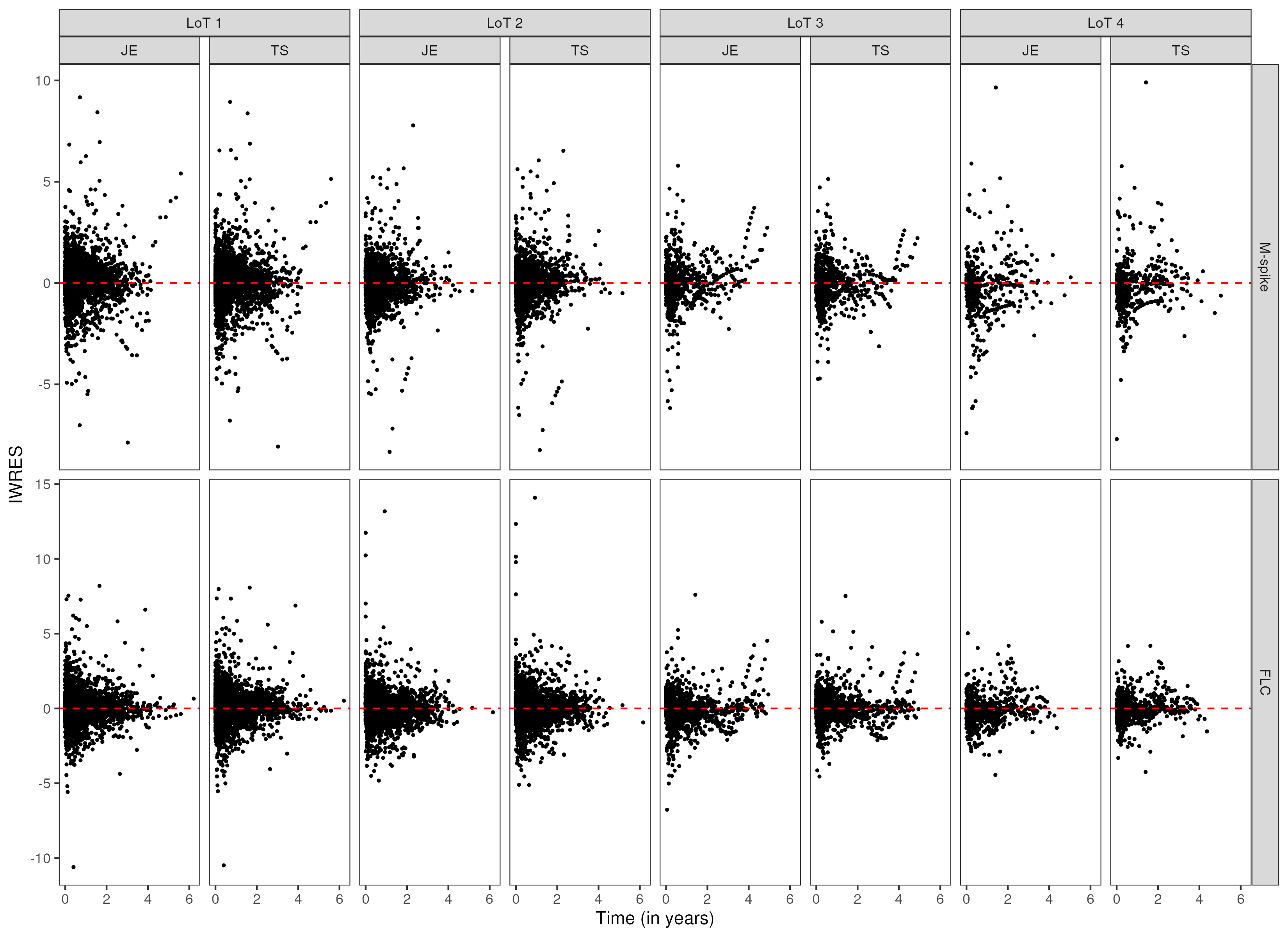
Figure 3: Individual weighted residuals (IWRES) from the bi-exponential submodel for each biomarker considering the test data set by line of therapy (LoT) using joint estimation (JE) and corrected two-stage (TS) approaches.

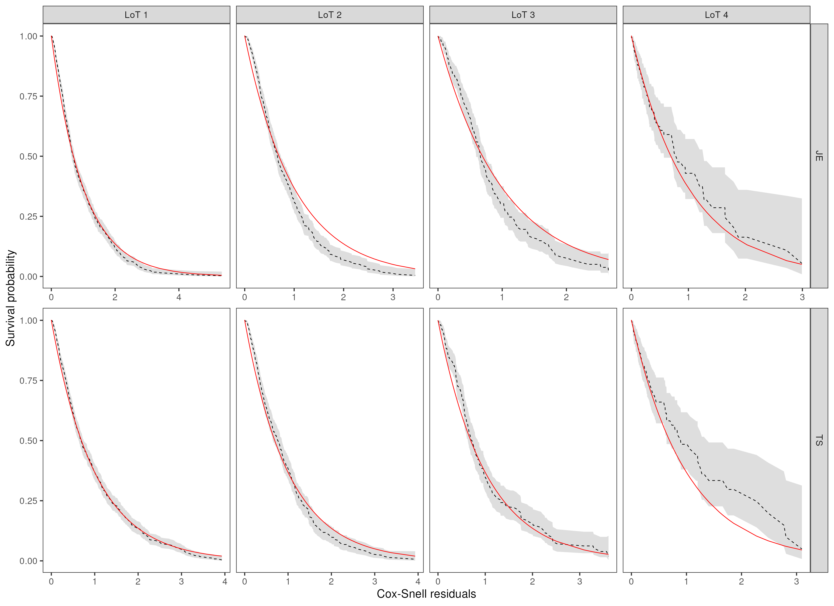
Figure 4: Kaplan–Meier estimates of the Cox–Snell residuals (dashed black line) and its 95% confidence interval (gray shadow) from the survival submodel considering the test data set by line of therapy (LoT) using joint estimation (JE) and corrected two-stage (TS) approaches. Solid red line: the survival function of the unit exponential distribution.

We evaluated the performance of the joint model (1)-(2) considering the test data set using joint estimation (JE) and corrected two-stage (TS) approaches. In summary, JE and TS achieved similar and satisfactory performance in all metrics, especially before LoT 4. For longitudinal submodel fit, IWRES suggested that a bi-exponential specification was suitable for modelling M-spike and FLC along LoTs using JE or TS (see Web Figure 3). For survival submodel fit, Cox-Snell residuals indicated a better fit using TS in LoTs 1, 2 & 3 (see Web Figure 4). For LoT 4, both estimation methods showed poor goodness-of-fit, with a small advantage in favor of JE, which has its curve closest to a unit exponential survival model (theoretical distribution). We hypothesise that many patients die or are censored after LoT 4 (362 cases, i.e., 50.5% of patients in LoT 4) and so biomarker trajectories (in LoT 4) are not informative for predicting time-to-death for such patients. For prediction evaluation, time-dependent AUCs showed similar discrimination results between two estimation methods, with the exception of LoT 3 for the time-to-death submodel (see Figure 2). We also find that at later landmarks, it is harder to discriminate between them. Finally, calibration plots assessed the agreement between predicted and observed risk using JE and TS, where highly comparable results were observed (see Figure 3 and Web Figure 5 for a comparison between JS and TS by decile and tercile of predicted 1-year risk, respectively).

5.2 Comparison of JE vs TS Model Fit

The estimation of longitudinal parameters seemed relatively similar using JE and TS approaches (see Web Tables 4 and 5). However, substantial differences were observed in the posterior mean trajectories for M-spike and FLC in each LoT (see Web Figure 6). In all cases, JE presented wider credible intervals, which is an expected result, since simultaneous inference considers more sources of uncertainty. Furthermore, the posterior mean trajectories using JE were above those estimated with TS, which is a finding of the influence of time-to-event information when estimating the longitudinal parameters. For the survival submodels, JE and TS produced similar results for both time-to-death (see Web Tables 6 and 7) and time-to-next-LoT (see Web Tables 8 and 9).

We highlight below common findings across the four LoTs for each clinical outcome. For time-to-death, patients who are older, with ECOG status 2⁺, low platelet count, high initial M-spike value, or high initial FLC value (in each LoT) have a higher risk of death. For time-to-next-LoT, patients who are non-Hispanic white, young, with low immunoglobulin G levels, short time spent in the previous LoT, high initial M-spike value, high initial FLC value, high growth rate for M-spike, or high growth rate for FLC (in each LoT) have a higher risk of starting a next LoT.

5.3 Dynamic Risk Prediction Examples

To illustrate individual dynamic predictions, i.e., predictions that are updated once more information becomes available for the patient, we randomly selected two patients, named A and B, whose baseline characteristics are presented in Web Table 10.

One-year dynamic predictions by using different lengths of histories of the respective patient ($t_{1}=$ first longitudinal observation, $t_{2}=$ up to 50% of longitudinal observations, and $t_{3}=$ up to the last longitudinal observation) are shown using TS (Figures 4 and 5) and JE (Web Figures 7 and 8) approaches. Comparatively, TS or JE are largely similar.

For patient A (Figure 4), M-spike and FLC decline over the first two LoTs, which could explain the fact that competing events have similar probabilities of occurrence and less than 50%. This behaviour is maintained for the first two landmark time points in LoT 3, until both biomarkers begin to increase their values (M-spike more quickly) and then the probability of the patient requiring a change of LoT also increases. In LoT 4, biomarkers resume their downward trend, which helps reduce the probability of death for patient A over time.

For patient B (Figure 5), M-spike value drops abruptly between the first and second measurement in LoT 1, while FLC values decrease slightly. Such behaviours reduce the probability of starting a next LoT and keep both competing events with a probability of occurrence between 20% and 30%. Note that the initiation of LoT 2 is started approximately after one year without longitudinal follow-up of the patient. In LoT 2, although both biomarkers present significant reductions, the risk of changing to LoT 3 remains around 50%. Patient B has low biomarker values over the first few months on line 3 of therapy, but her last M-spike and FLC measurements rise rapidly, which likely explains the increase at risk of starting a next LoT. In LoT 4, M-spike values remain more or less stable around 10 g/L while FLC values increase over time. Both biomarker trajectories combined with the baseline characteristics of patient B increase her risk of death.

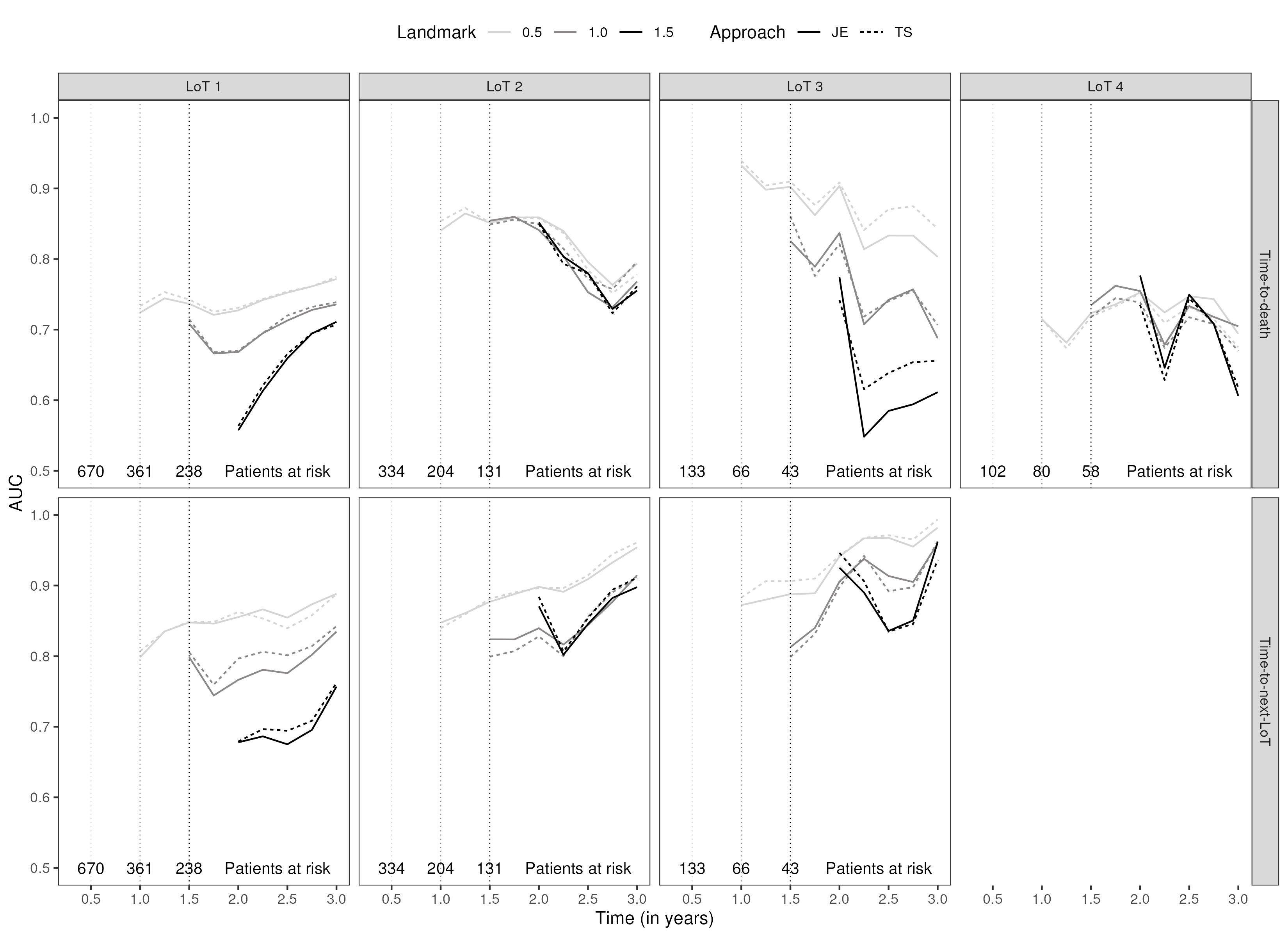
Figure 2: Time-dependent AUC from 6 months after landmark times at $0.5$, $1.0$, and $1.5$ years (from lightest to darkest respectively) for each time-to-event considering the test data set by line of therapy (LoT) using joint estimation (JE, solid line) and corrected two-stage (TS, dashed line) approaches.

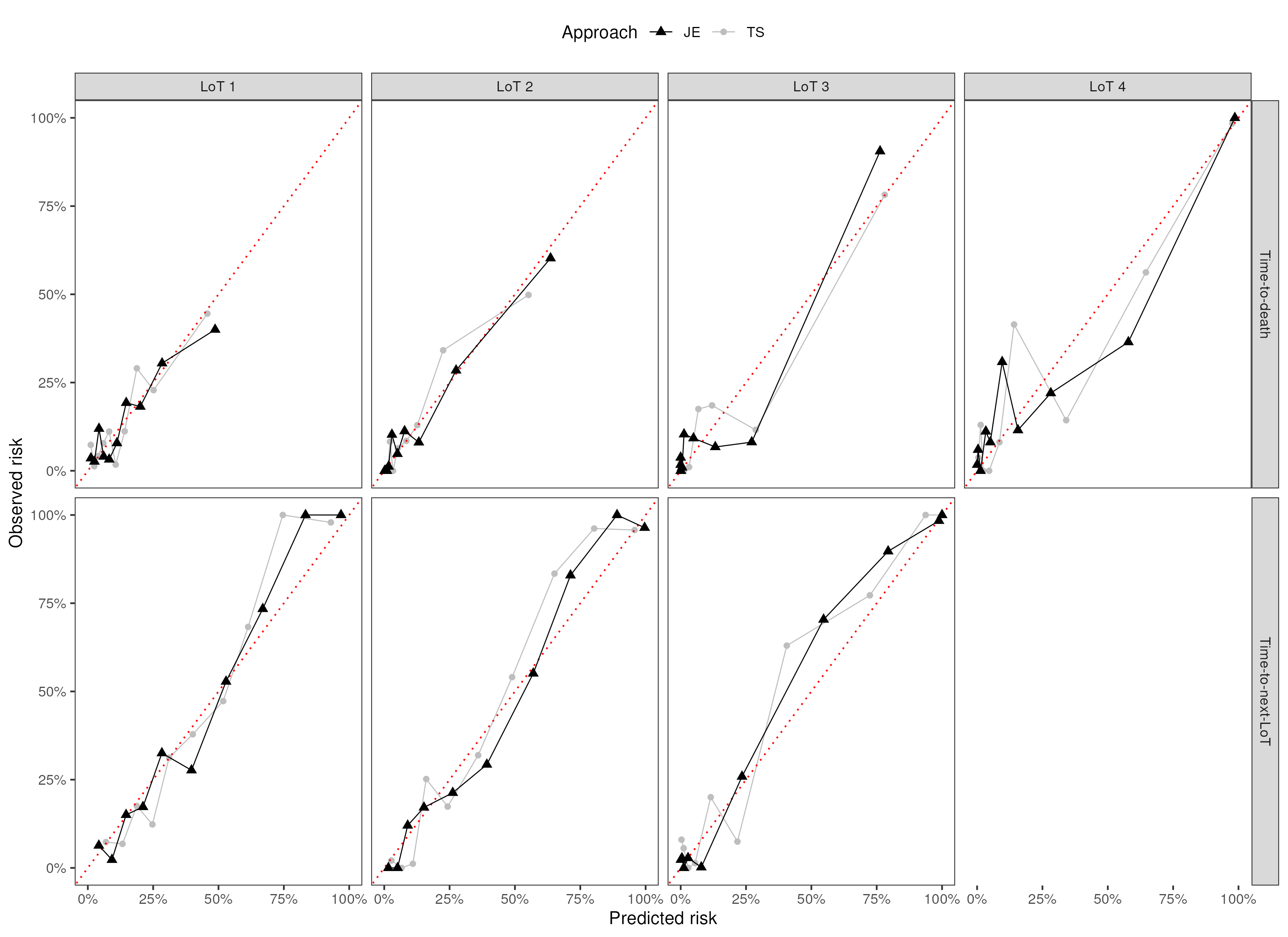
Figure 3: Calibration plots by decile of predicted 1-year risk from the survival submodel with 6 months of landmark time for each time-to-event considering the test data set by line of therapy (LoT) using joint estimation (JE, black triangle) and corrected two-stage (TS, gray circle) approaches.

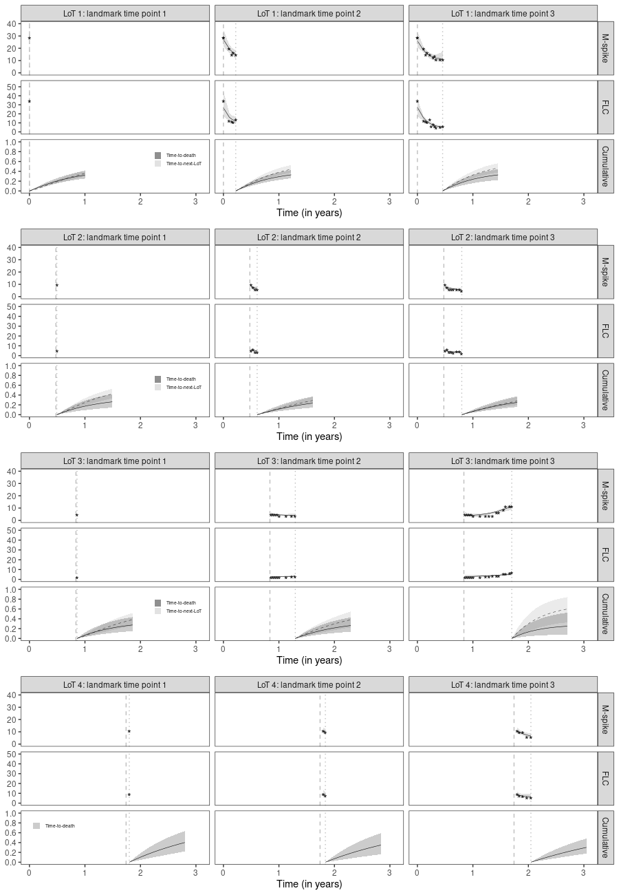
Figure 4: One-year dynamic predictions from three landmark time points (vertical dotted lines) in each line of therapy (LoT) using the corrected two-stage (TS) approach for patient A. Vertical dashed lines indicate LoT initiation times. For “M-spike” and “FLC” rows, stars represent biomarker observed values with their respective posterior mean trajectory (solid lines) and 95% credible intervals (gray shadow). For “Cumulative” rows, solid and dashed lines are posterior means (with their respective 95% credible intervals) of cumulative incidence functions (LoTs 1, 2 & 3) or distribution functions (LoT 4) for time-to-death and time-to-next-LoT, respectively.

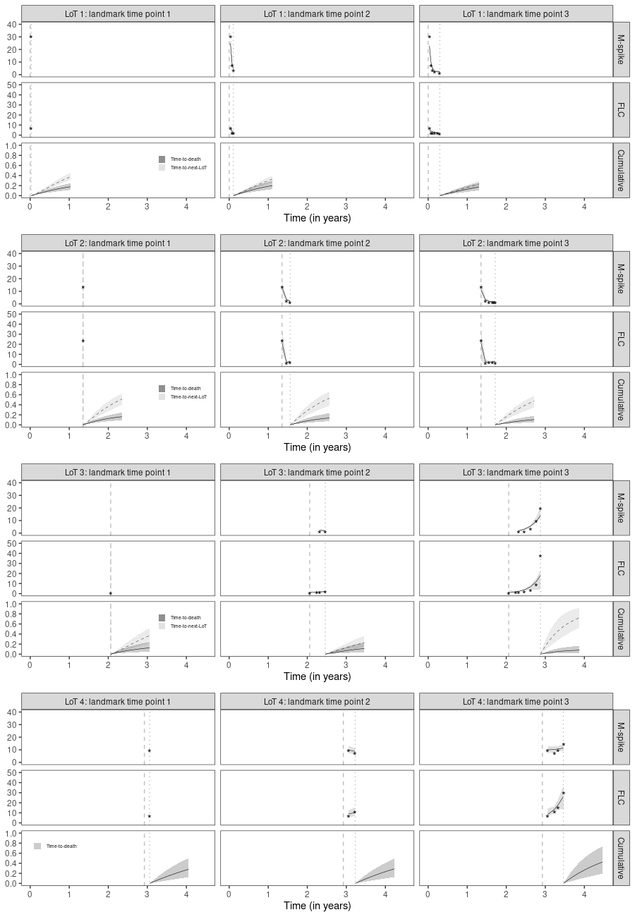
Figure 5: One-year dynamic predictions from three landmark time points (vertical dotted lines) in each line of therapy (LoT) using the corrected two-stage (TS) approach for patient B. Vertical dashed lines indicate LoT initiation times. For “M-spike” and “FLC” rows, stars represent biomarker observed values with their respective posterior mean trajectory (solid lines) and 95% credible intervals (gray shadow). For “Cumulative” rows, solid and dashed lines are posterior means (with their respective 95% credible intervals) of cumulative incidence functions (LoTs 1, 2 & 3) or distribution functions (LoT 4) for time-to-death and time-to-next-LoT, respectively.

6 Discussion

We have proposed a new Bayesian joint model for MM data that captures the dynamics of multiple biomarkers (M-spike and free light chains) through nonlinear mixed-effect submodels and shares characteristics of such biomarkers with a competing risks submodel, where the events of interest are death and change to next line of therapy. As an alternative to joint estimation (JE), we have extended the corrected two-stage (TS) approach proposed by Alvares and Leiva-Yamaguchi (2023) to this more complex joint model.

Model performance was evaluated using analyses of residuals and predictive performance metrics. Longitudinal residuals demonstrated satisfactory model fit for both JE and TS approaches, but Cox-Snell residuals indicated poor fit except for the first three lines of therapy using TS estimation. In addition, time-dependent AUCs and calibration plots have shown equally good predictive performance for both approaches. Moreover, posterior inferences presented similar conclusions regardless of the estimation approach used, but TS has required much less computational effort (46.5% reduction in processing time with 15.4 hours using TS vs 28.8 hours using JE).

We have revisited the dynamic prediction scheme for joint models introduced by Rizopoulos (2011) and discussed the minor modifications required to use it with the corrected two-stage estimation. We have also illustrated the applicability of dynamic risk predictions as an essential tool to better understand prognostic factors and their short-term and long-term impacts on patient journeys. For example, such predictions may inform optimal treatment strategies by risk status, support clinical decision-making at the point of care, and provide insights for clinical trial designs.

In conclusion, we have contributed to both hematology and statistical modelling literature with a new Bayesian predictive joint model that incorporates dynamic information from biomarker trajectories into a competing risks submodel. Our joint model can be extended in different directions, such as multiple change-points in more complex longitudinal data and multistate specifications. Furthermore, we would like to discuss some issues not covered in this work but which may be motivation for future research. For simplicity, we have handled missing data using the mean-value imputation, but other more sophisticated approaches could be explored, such as multiple imputation and machine learning techniques (Emmanuel et al., 2021). We have opted to use the well-known and popular dynamic prediction strategy proposed by Rizopoulos (2011), but existing literature also provides alternatives to dynamically update predictions when new longitudinal measurements become available, such as sequential Monte Carlo methods (Alvares et al., 2021). From a computational optimisation perspective, integrated nested Laplace approximation (Rue et al., 2009) is an alternative to speed up the inferential process for both JE and TS approaches. However, to the best of our knowledge, there are no implementations available yet for a joint model of multiple bi-exponential longitudinal submodels sharing their random effects with a competing risks submodel (van Niekerk et al., 2021, 2023; Alvares et al., 2024). Another option, especially for big datasets, is to use the approach proposed by Afonso et al. (2023), where data is divided into subsamples, joint models are fitted to each of them in parallel, and then a consensus distribution strategy is applied to unify the results. From a clinical perspective, the treatment regimen in each LoT can also be considered as a predictor. However, in our study, when incorporating such a regimen into the survival submodel there were no improvements in predictions, so we dropped it in the main analysis. It is also worth mentioning that starting a new LoT (one of the competing events) is a human decision that presumably involves multiple factors not considered in this work, such as comorbidities, aggressive clinical features, prior toxicities, treatment guidelines, etc. (Laubach et al., 2016; Mikhael et al., 2019; Dimopoulos et al., 2021). Hence, we hope that in the future such information will be available to be incorporated into the modelling process.

Data availability statement

For eligible studies qualified researchers may request access to individual patient-level clinical data through a data request platform. For up-to-date details on Roche’s Global Policy on the Sharing of Clinical Information and how to request access to related clinical study documents, see the website (https://go.roche.com/data_sharing). Anonymised records for individual patients across more than one data source external to Roche cannot, and should not, be linked due to a potential increase in risk of patient re-identification. The data that support the findings of this study were originated by and are the property of Flatiron Health, Inc., which has restrictions prohibiting the authors from making the data set publicly available. Requests for data sharing by license or by permission for the specific purpose of replicating results in this manuscript can be submitted to PublicationsDataAccess@flatiron.com. The data are subject to a license agreement with Flatiron Health to protect patient privacy and ensure compliance with measures necessary to reduce the risk of re-identification. For example, the data necessary to replicate the study include numerous specific dates, including visit dates (i.e., laboratory or examination dates), treatment start and stop dates, and month of death, as well as laboratory test results. Other measures to maintain de-identification without contractual agreements in place are not feasible due to the study question, methods used, and data elements required.

SUPPLEMENTARY MATERIAL

Appendix A. Web Tables

Table 1: Summary of the distribution of the number of M-spike and FLC measurements per patient by line of therapy (LoT).

Biomarker	Summary	LoT 1	LoT 2	LoT 3	LoT 4
M-spike	Min	1	1	1	1
	Quartile 1	2	2	2	2
	Median	4	4	3	3
	Quartile 3	6	7	7	7
	Max	97	53	66	43
FLC	Min	1	1	1	1
	Quartile 1	2	2	2	2
	Median	4	5	4	4
	Quartile 3	8	10	9	8
	Max	78	76	69	55

Table 2: Summary (number of cases and percentage) of categorical variables by line of therapy (LoT). In terms of modelling, the first category of each variable is defined as the reference category.

Baseline variable	LoT 1	LoT 2	LoT 3	LoT 4
Sex
Male	2981 (54.3%)	1536 (55.4%)	756 (54.0%)	395 (55.2%)
Female	2509 (45.7%)	1239 (44.6%)	645 (46.0%)	321 (44.8%)
Ethnicity
Non-Hispanic white	3063 (55.8%)	1613 (58.1%)	838 (59.8%)	437 (61.0%)
Non-Hispanic black	906 (16.5%)	445 (16.0%)	217 (15.5%)	109 (15.2%)
Other	960 (17.5%)	486 (17.5%)	239 (17.1%)	114 (15.9%)
Not reported	561 (10.2%)	231 (8.3%)	107 (7.6%)	56 (7.8%)
ECOG
0	1166 (21.2%)	597 (21.5%)	303 (21.6%)	142 (19.8%)
1	1382 (25.2%)	694 (25.0%)	358 (25.6%)	190 (26.5%)
2+	781 (14.2%)	361 (13.0%)	163 (11.6%)	77 (10.8%)
Not reported	2161 (39.4%)	1123 (40.5%)	577 (41.2%)	307 (42.9%)
ISS
Stage I	1144 (20.8%)	581 (20.9%)	282 (20.1%)	141 (19.7%)
Stage II	1129 (20.6%)	588 (21.2%)	299 (21.3%)	142 (19.8%)
Stage III	1141 (20.8%)	630 (22.7%)	337 (24.1%)	192 (26.8%)
Not reported	2076 (37.8%)	976 (35.2%)	483 (34.5%)	241 (33.7%)

Table 3: Summary of continuous variables in their original scales (Initial) and after log transformation¹¹, standardisation, and imputation²² (Final). NA represents the number of missing observations before imputation.

Baseline variable	Data	Mean	SD3	Median	Min	Max	NA (%)
Age	Initial	67.92	10.32	69.00	24.00	84.00	–
(years)	Final	0.00	1.00	0.17	-6.18	1.36	–
Albumin	Initial	36.12	12.02	38.00	0.04	519.00	1512 (28)
(serum, g/L)	Final	0.00	0.85	0.03	-10.95	5.46	–
B2M	Initial	10.01	103.88	4.00	0.20	3800.00	3041 (55)
(serum, mg/L)	Final	0.00	0.67	0.00	-3.75	9.22	–
Creatinine	Initial	1.51	1.85	1.10	0.40	83.00	1546 (28)
(serum, mg/dL)	Final	0.00	0.85	0.00	-1.95	8.09	–
Hemoglobin	Initial	10.78	2.17	10.70	3.10	22.50	736 (13)
(g/dL)	Final	0.00	0.93	0.00	-5.87	3.67	–
LDH	Initial	230.25	195.33	179.00	50.00	3182.00	3426 (62)
(serum, U/L)	Final	0.00	0.61	0.00	-2.72	5.53	–
Lymphocyte	Initial	1.82	1.23	1.60	0.00	32.70	1614 (29)
(count, $\times 10^{9}$/L)	Final	0.00	0.84	0.00	-5.87	6.12	–
Neutrophil	Initial	5.93	87.97	3.50	0.00	4758.00	2252 (41)
(count, $\times 10^{9}$/L)	Final	0.00	0.77	0.00	-6.32	12.75	–
Platelet	Initial	227.11	93.23	217.00	0.00	921.00	1635 (30)
(count, $\times 10^{9}$/L)	Final	0.00	0.84	0.00	-17.22	3.35	–
IgA	Initial	7.04	14.81	0.67	0.00	136.00	2663 (49)
(serum, g/L)	Final	0.00	0.72	0.00	-1.52	2.71	–
IgG	Initial	26.39	25.36	17.09	0.40	139.01	2544 (46)
(serum, g/L)	Final	0.00	0.73	0.00	-3.01	1.94	–
IgM	Initial	0.51	3.11	0.24	0.00	97.43	3105 (57)
(serum, g/L)	Final	0.00	0.66	0.00	-1.95	8.49	–

• $\log(x+0.1)$ to avoid numerical problems when $x=0$.

• Mean-value imputation strategy for missing values (Donders et al., 2006), i.e., we replace them with zeros (after standardisation, the mean of each variable is zero).

• After standardisation, the standard deviation is equal to 1, but the imputation concentrates more values at zero and consequently reduces such standard deviation.

Table 4: Posterior summary (mean and 95% credible interval) of the bi-exponential submodel parameters for each biomarker by line of therapy (LoT) using the joint estimation (JE) approach. Statistically significant variables are shown in bold, except for variance parameters.

Interpretation	Parameter	LoT $\bm{l=1}$	LoT $\bm{l=2}$	LoT $\bm{l=3}$	LoT $\bm{l=4}$
M-spike ($k=1$)
Baseline	$\exp\{\theta_{1kl}\}$	17.086 (16.405, 17.797)	7.765 (7.347, 8.232)	7.382 (6.780, 8.057)	7.950 (7.030, 8.971)
Growth	$\exp\{\theta_{2kl}\}$	0.246 (0.234, 0.259)	0.293 (0.257, 0.332)	0.377 (0.311, 0.450)	0.235 (0.158, 0.331)
Decay	$\exp\{\theta_{3kl}\}$	4.056 (3.815, 4.300)	1.092 (0.918, 1.295)	1.200 (0.921, 1.505)	0.924 (0.621, 1.327)
Residual error variance	$\sigma^{2}_{kl}$	0.053 (0.051, 0.054)	0.050 (0.048, 0.052)	0.061 (0.057, 0.064)	0.053 (0.049, 0.057)
	$\omega_{11kl}$	0.865 (0.806, 0.928)	0.922 (0.841, 1.011)	1.025 (0.903, 1.160)	1.033 (0.866, 1.231)
Covariance	$\omega_{12kl}$	-0.146 (-0.197, -0.094)	0.022 (-0.083, 0.128)	-0.160 (-0.325, 0.001)	-0.160 (-0.476, 0.150)
matrix for	$\omega_{13kl}$	0.595 (0.521, 0.672)	0.776 (0.621, 0.946)	0.701 (0.489, 0.933)	0.655 (0.314, 1.052)
random effects	$\omega_{22kl}$	0.709 (0.641, 0.781)	1.134 (0.966, 1.328)	1.182 (0.961, 1.455)	1.994 (1.401, 2.842)
	$\omega_{23kl}$	0.044 (-0.017, 0.106)	0.755 (0.549, 0.981)	0.385 (0.100, 0.708)	1.424 (0.770, 2.285)
	$\omega_{33kl}$	1.229 (1.114, 1.350)	2.621 (2.184, 3.116)	1.977 (1.509, 2.567)	2.986 (2.048, 4.321)
Free light chains ($k=2$)
Baseline	$\exp\{\theta_{1kl}\}$	20.748 (19.340, 22.189)	9.381 (8.662, 10.178)	10.246 (9.075, 11.575)	14.002 (11.646, 17.098)
Growth	$\exp\{\theta_{2kl}\}$	0.162 (0.149, 0.177)	0.342 (0.300, 0.388)	0.426 (0.350, 0.518)	0.392 (0.284, 0.517)
Decay	$\exp\{\theta_{3kl}\}$	2.903 (2.651, 3.164)	0.916 (0.736, 1.121)	1.109 (0.797, 1.499)	0.997 (0.590, 1.589)
Residual error variance	$\sigma^{2}_{kl}$	0.100 (0.097, 0.102)	0.075 (0.072, 0.077)	0.080 (0.076, 0.083)	0.102 (0.095, 0.109)
	$\omega_{11kl}$	3.017 (2.841, 3.198)	2.330 (2.150, 2.524)	2.525 (2.248, 2.827)	2.792 (2.375, 3.275)
Covariance	$\omega_{12kl}$	-1.199 (-1.332, -1.072)	0.076 (-0.083, 0.234)	0.247 (-0.023, 0.518)	-0.052 (-0.464, 0.358)
matrix for	$\omega_{13kl}$	1.914 (1.749, 2.095)	1.874 (1.616, 2.148)	1.851 (1.463, 2.289)	2.099 (1.453, 2.872)
random effects	$\omega_{22kl}$	1.477 (1.340, 1.623)	1.928 (1.701, 2.185)	2.335 (1.945, 2.791)	2.263 (1.725, 2.941)
	$\omega_{23kl}$	0.038 (-0.105, 0.183)	1.354 (1.055, 1.683)	1.582 (1.102, 2.144)	1.025 (0.293, 1.875)
	$\omega_{33kl}$	2.980 (2.726, 3.268)	4.473 (3.821, 5.210)	4.364 (3.415, 5.525)	5.008 (3.518, 7.075)

Table 5: Posterior summary (mean and 95% credible interval) of the bi-exponential submodel parameters for each biomarker by line of therapy (LoT) using the corrected two-stage (TS) approach. Statistically significant variables are shown in bold, except for variance parameters.

Interpretation	Parameter	LoT $\bm{l=1}$	LoT $\bm{l=2}$	LoT $\bm{l=3}$	LoT $\bm{l=4}$
M-spike ($k=1$)
Baseline	$\exp\{\theta_{1kl}\}$	16.841 (16.197, 17.546)	7.675 (7.250, 8.160)	7.388 (6.792, 8.047)	7.786 (6.920, 8.759)
Growth	$\exp\{\theta_{2kl}\}$	0.196 (0.185, 0.207)	0.220 (0.191, 0.249)	0.283 (0.231, 0.344)	0.215 (0.139, 0.306)
Decay	$\exp\{\theta_{3kl}\}$	3.624 (3.401, 3.858)	0.910 (0.763, 1.080)	1.049 (0.827, 1.310)	0.874 (0.562, 1.283)
Residual error variance	$\sigma^{2}_{kl}$	0.053 (0.051, 0.054)	0.051 (0.049, 0.053)	0.061 (0.058, 0.064)	0.053 (0.049, 0.057)
	$\omega_{11kl}$	0.865 (0.808, 0.927)	0.917 (0.838, 1.004)	1.013 (0.894, 1.146)	1.030 (0.860, 1.232)
Covariance	$\omega_{12kl}$	-0.135 (-0.193, -0.079)	-0.035 (-0.162, 0.087)	-0.206 (-0.389, -0.024)	-0.165 (-0.485, 0.147)
matrix for	$\omega_{13kl}$	0.631 (0.554, 0.711)	0.766 (0.604, 0.941)	0.672 (0.452, 0.909)	0.663 (0.316, 1.063)
random effects	$\omega_{22kl}$	0.661 (0.592, 0.737)	1.292 (1.079, 1.537)	1.358 (1.066, 1.705)	2.031 (1.407, 2.931)
	$\omega_{23kl}$	0.196 (0.124, 0.272)	0.981 (0.735, 1.258)	0.595 (0.265, 0.977)	1.456 (0.763, 2.399)
	$\omega_{33kl}$	1.422 (1.294, 1.562)	2.911 (2.449, 3.449)	2.173 (1.657, 2.793)	3.028 (2.018, 4.394)
Free light chains ($k=2$)
Baseline	$\exp\{\theta_{1kl}\}$	19.802 (18.528, 21.254)	8.915 (8.184, 9.663)	9.976 (8.779, 11.311)	13.173 (10.983, 15.915)
Growth	$\exp\{\theta_{2kl}\}$	0.143 (0.132, 0.155)	0.178 (0.148, 0.210)	0.196 (0.142, 0.260)	0.283 (0.198, 0.381)
Decay	$\exp\{\theta_{3kl}\}$	2.605 (2.374, 2.850)	0.506 (0.400, 0.631)	0.642 (0.445, 0.885)	0.767 (0.431, 1.222)
Residual error variance	$\sigma^{2}_{kl}$	0.100 (0.098, 0.102)	0.075 (0.073, 0.078)	0.080 (0.077, 0.084)	0.102 (0.095, 0.109)
	$\omega_{11kl}$	2.977 (2.810, 3.154)	2.318 (2.139, 2.511)	2.546 (2.277, 2.842)	2.782 (2.365, 3.259)
Covariance	$\omega_{12kl}$	-1.234 (-1.365, -1.105)	-0.106 (-0.333, 0.113)	-0.028 (-0.461, 0.378)	-0.230 (-0.681, 0.211)
matrix for	$\omega_{13kl}$	1.897 (1.729, 2.076)	1.905 (1.610, 2.223)	1.906 (1.446, 2.408)	2.053 (1.393, 2.826)
random effects	$\omega_{22kl}$	1.586 (1.438, 1.741)	2.464 (2.099, 2.905)	3.177 (2.494, 4.031)	2.432 (1.809, 3.270)
	$\omega_{23kl}$	0.144 (0.003, 0.290)	2.031 (1.571, 2.575)	2.547 (1.765, 3.531)	1.189 (0.395, 2.155)
	$\omega_{33kl}$	3.053 (2.787, 3.334)	5.569 (4.730, 6.598)	5.713 (4.383, 7.398)	5.319 (3.698, 7.546)

Table 6: Posterior summary (mean and 95% credible interval) for time-to-death ($v=1$) by line of therapy (LoT) using the joint estimation (JE) approach. Statistically significant variables are shown in bold.

Variable	Category	LoT $\bm{l=1}$	LoT $\bm{l=2}$	LoT $\bm{l=3}$	LoT $\bm{l=4}$
Sex	Female	-0.159 (-0.323, 0.006)	-0.339 (-0.579, -0.096)	-0.165 (-0.465, 0.134)	-0.307 (-0.627, 0.018)
Ethnicity	Non-Hisp. Black	-0.082 (-0.315, 0.143)	0.004 (-0.326, 0.326)	0.017 (-0.406, 0.426)	0.208 (-0.208, 0.602)
	Other	-0.012 (-0.237, 0.200)	-0.233 (-0.553, 0.071)	-0.355 (-0.779, 0.050)	-0.653 (-1.148, -0.177)
ECOG	1	0.174 (-0.093, 0.446)	0.051 (-0.320, 0.423)	-0.069 (-0.517, 0.379)	0.783 (0.321, 1.271)
	2+	0.806 (0.539, 1.086)	0.665 (0.285, 1.050)	0.610 (0.120, 1.107)	0.963 (0.358, 1.566)
ISS	Stage II	0.543 (0.207, 0.877)	0.197 (-0.227, 0.619)	-0.059 (-0.570, 0.471)	0.617 (0.090, 1.162)
	Stage III	0.464 (0.072, 0.858)	0.316 (-0.162, 0.797)	0.224 (-0.385, 0.849)	0.584 (-0.022, 1.214)
Age	–	0.557 (0.448, 0.671)	0.472 (0.322, 0.624)	0.560 (0.373, 0.755)	0.171 (0.019, 0.327)
Albumin	–	-0.073 (-0.163, 0.023)	0.056 (-0.125, 0.265)	-0.167 (-0.347, 0.030)	-0.078 (-0.320, 0.205)
B2M	–	0.244 (0.082, 0.397)	-0.005 (-0.227, 0.200)	-0.268 (-0.588, 0.029)	0.292 (-0.043, 0.623)
Creatine	–	0.036 (-0.064, 0.134)	0.053 (-0.099, 0.200)	0.055 (-0.152, 0.257)	-0.081 (-0.314, 0.148)
Hemoglobin	–	-0.125 (-0.220, -0.029)	-0.074 (-0.205, 0.059)	-0.131 (-0.297, 0.034)	0.091 (-0.089, 0.279)
LDH	–	0.153 (0.041, 0.263)	0.140 (-0.025, 0.296)	0.212 (-0.013, 0.420)	-0.038 (-0.262, 0.173)
Lymphocyte	–	-0.045 (-0.134, 0.045)	-0.030 (-0.166, 0.104)	-0.017 (-0.170, 0.138)	-0.056 (-0.230, 0.121)
Neutrophil	–	0.169 (0.061, 0.278)	0.178 (0.018, 0.332)	0.019 (-0.166, 0.211)	0.165 (-0.049, 0.380)
Platelet	–	-0.091 (-0.162, -0.011)	-0.080 (-0.232, 0.072)	-0.178 (-0.357, 0.008)	-0.318 (-0.513, -0.125)
IgA	–	0.015 (-0.125, 0.157)	0.279 (0.089, 0.469)	0.158 (-0.076, 0.389)	-0.135 (-0.361, 0.093)
IgG	–	0.129 (-0.010, 0.269)	0.172 (-0.033, 0.376)	-0.024 (-0.267, 0.221)	-0.273 (-0.492, -0.050)
IgM	–	0.163 (0.043, 0.279)	0.078 (-0.091, 0.227)	-0.076 (-0.324, 0.147)	-0.116 (-0.310, 0.082)
Time prev. LoT	–	–	-0.043 (-0.169, 0.078)	-0.188 (-0.388, -0.004)	-0.298 (-0.578, -0.039)
Baseline M-spike ($\alpha_{1lk1}$)	–	0.206 (0.055, 0.359)	0.297 (0.105, 0.490)	0.134 (-0.127, 0.397)	0.450 (0.146, 0.778)
Growth M-spike ($\alpha_{1lk2}$)	–	0.382 (0.197, 0.566)	-0.049 (-0.293, 0.201)	0.198 (-0.142, 0.530)	0.240 (-0.181, 0.680)
Decay M-spike ($\alpha_{1lk3}$)	–	-0.014 (-0.145, 0.116)	-0.036 (-0.191, 0.117)	0.053 (-0.201, 0.304)	-0.111 (-0.445, 0.205)
Baseline FLC ($\alpha_{2lk1}$)	–	0.103 (-0.035, 0.236)	0.290 (0.162, 0.413)	0.253 (0.077, 0.428)	0.221 (0.055, 0.390)
Growth FLC ($\alpha_{2lk2}$)	–	0.107 (-0.069, 0.273)	0.476 (0.307, 0.641)	0.164 (-0.054, 0.383)	0.413 (0.212, 0.609)
Decay FLC ($\alpha_{2lk3}$)	–	0.099 (-0.014, 0.215)	-0.001 (-0.131, 0.135)	-0.070 (-0.263, 0.117)	0.017 (-0.162, 0.195)

Table 7: Posterior summary (mean and 95% credible interval) for time-to-death ($v=1$) by line of therapy (LoT) using the corrected two-stage (TS) approach. Statistically significant variables are shown in bold.

Variable	Category	LoT $\bm{l=1}$	LoT $\bm{l=2}$	LoT $\bm{l=3}$	LoT $\bm{l=4}$
Sex	Female	-0.155 (-0.316, 0.004)	-0.315 (-0.547, -0.078)	-0.152 (-0.438, 0.143)	-0.290 (-0.598, 0.017)
Ethnicity	Non-Hisp. Black	-0.087 (-0.315, 0.152)	-0.009 (-0.319, 0.314)	0.041 (-0.382, 0.451)	0.197 (-0.195, 0.588)
	Other	0.002 (-0.210, 0.214)	-0.235 (-0.548, 0.082)	-0.356 (-0.753, 0.039)	-0.619 (-1.129, -0.144)
ECOG	1	0.158 (-0.105, 0.452)	0.052 (-0.311, 0.438)	-0.039 (-0.519, 0.413)	0.768 (0.344, 1.253)
	2+	0.789 (0.523, 1.069)	0.658 (0.290, 1.064)	0.647 (0.134, 1.158)	0.933 (0.359, 1.519)
ISS	Stage II	0.545 (0.216, 0.888)	0.209 (-0.204, 0.625)	-0.034 (-0.532, 0.490)	0.588 (0.050, 1.139)
	Stage III	0.472 (0.075, 0.874)	0.368 (-0.101, 0.847)	0.238 (-0.381, 0.870)	0.598 (-0.022, 1.206)
Age	–	0.555 (0.443, 0.665)	0.457 (0.307, 0.605)	0.572 (0.385, 0.771)	0.163 (0.005, 0.327)
Albumin	–	-0.067 (-0.152, 0.026)	0.046 (-0.133, 0.245)	-0.165 (-0.347, 0.051)	-0.079 (-0.320, 0.209)
B2M	–	0.239 (0.075, 0.391)	-0.002 (-0.211, 0.198)	-0.292 (-0.597, 0.003)	0.284 (-0.036, 0.610)
Creatine	–	0.041 (-0.058, 0.136)	0.050 (-0.088, 0.190)	0.054 (-0.151, 0.252)	-0.100 (-0.323, 0.110)
Hemoglobin	–	-0.123 (-0.211, -0.027)	-0.075 (-0.218, 0.059)	-0.133 (-0.305, 0.038)	0.071 (-0.105, 0.254)
LDH	–	0.161 (0.046, 0.274)	0.145 (-0.016, 0.292)	0.217 (-0.007, 0.420)	-0.037 (-0.262, 0.170)
Lymphocyte	–	-0.040 (-0.125, 0.044)	-0.001 (-0.123, 0.131)	-0.019 (-0.159, 0.131)	-0.066 (-0.228, 0.110)
Neutrophil	–	0.168 (0.067, 0.272)	0.178 (0.022, 0.333)	0.027 (-0.155, 0.206)	0.169 (-0.040, 0.367)
Platelet	–	-0.093 (-0.161, -0.013)	-0.105 (-0.250, 0.050)	-0.206 (-0.401, -0.007)	-0.320 (-0.509, -0.133)
IgA	–	0.020 (-0.121, 0.165)	0.283 (0.098, 0.468)	0.171 (-0.063, 0.405)	-0.126 (-0.344, 0.104)
IgG	–	0.120 (-0.016, 0.256)	0.179 (-0.018, 0.374)	-0.011 (-0.261, 0.237)	-0.267 (-0.486, -0.043)
IgM	–	0.162 (0.042, 0.276)	0.088 (-0.070, 0.242)	-0.081 (-0.332, 0.150)	-0.117 (-0.294, 0.066)
Time prev. LoT	–	–	-0.027 (-0.143, 0.084)	-0.182 (-0.384, 0.003)	-0.300 (-0.580, -0.064)
Baseline M-spike ($\alpha_{1lk1}$)	–	0.197 (0.030, 0.350)	0.308 (0.100, 0.510)	0.140 (-0.116, 0.403)	0.466 (0.172, 0.758)
Growth M-spike ($\alpha_{1lk2}$)	–	0.245 (0.041, 0.438)	-0.065 (-0.298, 0.198)	0.123 (-0.180, 0.425)	0.266 (-0.093, 0.658)
Decay M-spike ($\alpha_{1lk3}$)	–	-0.046 (-0.177, 0.087)	-0.031 (-0.181, 0.125)	0.013 (-0.216, 0.251)	-0.127 (-0.440, 0.161)
Baseline FLC ($\alpha_{2lk1}$)	–	0.080 (-0.057, 0.218)	0.309 (0.176, 0.443)	0.236 (0.058, 0.419)	0.240 (0.085, 0.400)
Growth FLC ($\alpha_{2lk2}$)	–	0.061 (-0.111, 0.231)	0.282 (0.111, 0.440)	0.004 (-0.207, 0.225)	0.330 (0.152, 0.505)
Decay FLC ($\alpha_{2lk3}$)	–	0.098 (-0.021, 0.216)	-0.045 (-0.168, 0.081)	-0.055 (-0.241, 0.123)	-0.028 (-0.185, 0.136)

Table 8: Posterior summary (mean and 95% credible interval) for time-to-next-LoT ($v=2$) by line of therapy (LoT) using the joint estimation (JE) approach. Statistically significant variables are shown in bold.

Variable	Category	LoT $\bm{l=1}$	LoT $\bm{l=2}$	LoT $\bm{l=3}$
Sex	Female	-0.027 (-0.122, 0.069)	0.005 (-0.130, 0.140)	-0.185 (-0.379, 0.007)
Ethnicity	Non-Hisp. Black	-0.220 (-0.358, -0.086)	-0.109 (-0.297, 0.076)	-0.151 (-0.422, 0.110)
	Other	-0.050 (-0.180, 0.076)	-0.195 (-0.374, -0.014)	-0.454 (-0.727, -0.183)
ECOG	1	0.125 (-0.010, 0.263)	0.094 (-0.096, 0.286)	0.058 (-0.219, 0.341)
	2+	0.161 (-0.008, 0.327)	-0.094 (-0.336, 0.145)	0.125 (-0.236, 0.487)
ISS	Stage II	-0.027 (-0.179, 0.126)	0.048 (-0.163, 0.260)	-0.125 (-0.437, 0.189)
	Stage III	0.090 (-0.102, 0.285)	0.048 (-0.203, 0.302)	0.175 (-0.190, 0.534)
Age	–	-0.210 (-0.256, -0.164)	-0.124 (-0.187, -0.063)	-0.168 (-0.259, -0.076)
Albumin	–	0.005 (-0.054, 0.067)	-0.050 (-0.146, 0.053)	-0.034 (-0.188, 0.132)
B2M	–	0.068 (-0.035, 0.168)	-0.040 (-0.172, 0.089)	-0.098 (-0.278, 0.078)
Creatine	–	-0.028 (-0.096, 0.037)	-0.048 (-0.144, 0.045)	-0.011 (-0.148, 0.122)
Hemoglobin	–	-0.067 (-0.125, -0.010)	-0.002 (-0.080, 0.074)	0.020 (-0.095, 0.134)
LDH	–	-0.065 (-0.140, 0.009)	-0.047 (-0.152, 0.058)	0.019 (-0.137, 0.173)
Lymphocyte	–	0.035 (-0.021, 0.091)	-0.043 (-0.125, 0.039)	-0.009 (-0.114, 0.096)
Neutrophil	–	-0.054 (-0.118, 0.011)	-0.015 (-0.106, 0.075)	-0.075 (-0.198, 0.051)
Platelet	–	-0.008 (-0.061, 0.047)	-0.047 (-0.138, 0.044)	-0.075 (-0.196, 0.046)
IgA	–	-0.101 (-0.178, -0.025)	0.009 (-0.104, 0.116)	-0.043 (-0.185, 0.099)
IgG	–	-0.107 (-0.184, -0.030)	-0.045 (-0.155, 0.065)	-0.174 (-0.319, -0.030)
IgM	–	-0.064 (-0.139, 0.010)	-0.039 (-0.141, 0.056)	-0.099 (-0.244, 0.038)
Time prev. LoT	–	–	-0.113 (-0.190, -0.038)	-0.166 (-0.286, -0.049)
Baseline M-spike ($\alpha_{1lk1}$)	–	0.332 (0.233, 0.430)	0.311 (0.186, 0.437)	0.480 (0.299, 0.663)
Growth M-spike ($\alpha_{1lk2}$)	–	0.971 (0.855, 1.086)	0.631 (0.444, 0.814)	0.569 (0.375, 0.769)
Decay M-spike ($\alpha_{1lk3}$)	–	0.036 (-0.049, 0.122)	-0.070 (-0.180, 0.041)	-0.205 (-0.379, -0.035)
Baseline FLC ($\alpha_{2lk1}$)	–	0.277 (0.199, 0.354)	0.206 (0.122, 0.290)	0.256 (0.139, 0.376)
Growth FLC ($\alpha_{2lk2}$)	–	0.295 (0.183, 0.405)	0.483 (0.369, 0.599)	0.611 (0.468, 0.759)
Decay FLC ($\alpha_{2lk3}$)	–	-0.028 (-0.096, 0.040)	0.080 (-0.012, 0.173)	0.041 (-0.095, 0.179)

Table 9: Posterior summary (mean and 95% credible interval) for time-to-next-LoT ($v=2$) by line of therapy (LoT) using the corrected two-stage (TS) approach. Statistically significant variables are shown in bold.

Variable	Category	LoT $\bm{l=1}$	LoT $\bm{l=2}$	LoT $\bm{l=3}$
Sex	Female	-0.027 (-0.119, 0.063)	0.015 (-0.113, 0.140)	-0.195 (-0.381, -0.004)
Ethnicity	Non-Hisp. Black	-0.220 (-0.361, -0.092)	-0.127 (-0.327, 0.054)	-0.119 (-0.386, 0.139)
	Other	-0.021 (-0.152, 0.094)	-0.211 (-0.386, -0.042)	-0.494 (-0.767, -0.222)
ECOG	1	0.117 (-0.026, 0.256)	0.107 (-0.073, 0.284)	0.076 (-0.203, 0.351)
	2+	0.152 (-0.022, 0.321)	-0.079 (-0.313, 0.144)	0.119 (-0.240, 0.469)
ISS	Stage II	-0.002 (-0.152, 0.153)	0.051 (-0.159, 0.245)	-0.056 (-0.333, 0.244)
	Stage III	0.101 (-0.079, 0.288)	0.094 (-0.148, 0.335)	0.210 (-0.149, 0.568)
Age	–	-0.220 (-0.262, -0.178)	-0.141 (-0.200, -0.080)	-0.171 (-0.254, -0.087)
Albumin	–	0.009 (-0.047, 0.067)	-0.057 (-0.147, 0.038)	-0.055 (-0.206, 0.101)
B2M	–	0.062 (-0.033, 0.154)	-0.035 (-0.165, 0.082)	-0.123 (-0.305, 0.043)
Creatine	–	-0.019 (-0.083, 0.045)	-0.051 (-0.145, 0.041)	-0.003 (-0.140, 0.122)
Hemoglobin	–	-0.056 (-0.111, 0.003)	-0.001 (-0.073, 0.070)	0.019 (-0.091, 0.125)
LDH	–	-0.044 (-0.113, 0.026)	-0.053 (-0.157, 0.042)	0.023 (-0.118, 0.164)
Lymphocyte	–	0.035 (-0.021, 0.086)	-0.025 (-0.104, 0.052)	-0.013 (-0.120, 0.091)
Neutrophil	–	-0.050 (-0.111, 0.011)	-0.010 (-0.100, 0.080)	-0.061 (-0.183, 0.066)
Platelet	–	-0.012 (-0.061, 0.038)	-0.067 (-0.157, 0.021)	-0.099 (-0.220, 0.021)
IgA	–	-0.098 (-0.178, -0.018)	0.009 (-0.098, 0.115)	-0.027 (-0.170, 0.117)
IgG	–	-0.122 (-0.202, -0.045)	-0.044 (-0.149, 0.058)	-0.168 (-0.321, -0.013)
IgM	–	-0.063 (-0.138, 0.013)	-0.031 (-0.132, 0.067)	-0.099 (-0.237, 0.033)
Time prev. LoT	–	–	-0.107 (-0.185, -0.029)	-0.164 (-0.295, -0.041)
Baseline M-spike ($\alpha_{1lk1}$)	–	0.376 (0.288, 0.473)	0.367 (0.252, 0.488)	0.507 (0.340, 0.681)
Growth M-spike ($\alpha_{1lk2}$)	–	0.803 (0.692, 0.918)	0.561 (0.404, 0.724)	0.520 (0.338, 0.721)
Decay M-spike ($\alpha_{1lk3}$)	–	-0.063 (-0.137, 0.009)	-0.084 (-0.182, 0.016)	-0.229 (-0.386, -0.084)
Baseline FLC ($\alpha_{2lk1}$)	–	0.269 (0.192, 0.347)	0.253 (0.173, 0.337)	0.357 (0.243, 0.475)
Growth FLC ($\alpha_{2lk2}$)	–	0.243 (0.148, 0.337)	0.320 (0.220, 0.417)	0.452 (0.313, 0.594)
Decay FLC ($\alpha_{2lk3}$)	–	-0.037 (-0.105, 0.029)	0.005 (-0.077, 0.084)	-0.069 (-0.185, 0.047)

Table 10: Baseline variables of patients used to illustrate individual dynamic predictions.

Baseline variable	Patient A	Patient B
Sex	Male	Female
Ethnicity	Non-Hispanic white	Non-Hispanic white
ECOG	2+	0
ISS	Not reported	Stage III
Age (years)	72	73
Albumin (serum, g/L)	34	19
B2B (serum, mg/L)	NA	13.8
Creatinine (serum, mg/dL)	0.93	0.9
Hemoglobin (g/dL)	13.8	9.9
LDH (serum, U/L)	Not reported	308
Lymphocyte (count, $\times 10^{9}$/L)	0.847	1.5
Neutrophil (count, $\times 10^{9}$/L)	4.7	5.4
Platelet (count, $\times 10^{9}$/L)	233	215
IgA (serum, g/L)	NA	0.18
IgG (serum, g/L)	83	93.68
IgM (serum, g/L)	NA	0.15

Appendix B. Web Figures

Figure 5: Calibration plots by tercile of predicted 1-year risk from the survival submodel with 6 months of landmark time for each time-to-event considering the test data set by line of therapy (LoT) using joint estimation (JE, black triangle) and corrected two-stage (TS, gray circle) approaches.

Figure 6: Posterior mean trajectory and its 95% credible interval from the bi-exponential submodel for each biomarker by line of therapy (LoT) using joint estimation (JE, solid line) and corrected two-stage (TS, dashed line) approaches.

Figure 7: One-year dynamic predictions from three landmark time points (vertical dotted lines) in each line of therapy (LoT) using the joint estimation (JE) approach for patient A. Vertical dashed lines indicate LoT initiation times. For “M-spike” and “FLC” rows, stars represent biomarker observed values with their respective posterior mean trajectory (solid lines) and 95% credible intervals (gray shadow). For “Cumulative” rows, solid and dashed lines are posterior means (with their respective 95% credible intervals) of cumulative incidence functions (LoTs 1, 2 & 3) or distribution functions (LoT 4) for time-to-death and time-to-next-LoT, respectively.

Figure 8: One-year dynamic predictions from three landmark time points (vertical dotted lines) in each line of therapy (LoT) using the joint estimation (JE) approach for patient B. Vertical dashed lines indicate LoT initiation times. For “M-spike” and “FLC” rows, stars represent biomarker observed values with their respective posterior mean trajectory (solid lines) and 95% credible intervals (gray shadow). For “Cumulative” rows, solid and dashed lines are posterior means (with their respective 95% credible intervals) of cumulative incidence functions (LoTs 1, 2 & 3) or distribution functions (LoT 4) for time-to-death and time-to-next-LoT, respectively.

References

- Abdallah et al. (2023) Abdallah, N. H., Smith, A. N., Geyer, S., Binder, M., Greipp, P. T., Kapoor, P., Dispenzieri, A., Gertz, M. A., Baughn, L. B., Lacy, M. Q., Hayman, S. R., Buadi, F. K., Dingli, D., Hwa, Y. L., Lin, Y., Kourelis, T., Warsame, R., Kyle, R. A., Rajkumar, S. V., and Kumar, S. K. (2023). Conditional survival in multiple myeloma and impact of prognostic factors over time. Blood Cancer Journal 13, 1–8.
- Afonso et al. (2023) Afonso, P. M., Rizopoulos, D., Palipana, A. K., Zhou, G. C., Brokamp, C., Szczesniak, R. D., and Andrinopoulou, E. R. (2023). Efficiently analyzing large patient registries with Bayesian joint models for longitudinal and time-to-event data. arXiv:2310.03351 .
- Alsefri et al. (2020) Alsefri, M., Sudell, M., García-Fiñana, M., and Kolamunnage-Dona, R. (2020). Bayesian joint modelling of longitudinal and time to event data: a methodological review. BMC Medical Research Methodology 20, 1–17.
- Alvares et al. (2021) Alvares, D., Armero, C., Forte, A., and Chopin, N. (2021). Sequential Monte Carlo methods in Bayesian joint models for longitudinal and time-to-event data. Statistical Modelling 21, 161–181.
- Alvares and Leiva-Yamaguchi (2023) Alvares, D. and Leiva-Yamaguchi, V. (2023). A two-stage approach for Bayesian joint models: reducing complexity while maintaining accuracy. Statistics and Computing 3, 1–11.
- Alvares and Mercier (2024) Alvares, D. and Mercier, F. (2024). Bridging the gap between two-stage and joint models: the case of tumor growth inhibition and overall survival models. To appear in Statistics in Medicine .
- Alvares et al. (2024) Alvares, D., van Niekerk, J., Krainski, E. T., Rue, H., and Rustand, D. (2024). Bayesian survival analysis with INLA. arXiv:2212.01900 .
- Andrinopoulou et al. (2021) Andrinopoulou, E. R., Harhay, M. O., Ratcliffe, S. J., and Rizopoulos, D. (2021). Reflection on modern methods: dynamic prediction using joint models of longitudinal and time-to-event data. International Journal of Epidemiology 50, 1731–1743.
- Andrinopoulou et al. (2017) Andrinopoulou, E. R., Rizopoulos, D., Takkenberg, J. J. M., and Lesaffre, E. (2017). Combined dynamic predictions using joint models of two longitudinal outcomes and competing risk data. Statistical Methods in Medical Research 26, 1787–1801.
- Austin et al. (2022) Austin, P. C., Putter, H., Giardiello, D., and van Klaveren, D. (2022). Graphical calibration curves and the integrated calibration index (ICI) for competing risk models. Diagnostic and Prognostic Research 6, 1–22.
- Barrett and Su (2017) Barrett, J. and Su, L. (2017). Dynamic predictions using flexible joint models of longitudinal and time-to-event data. Statistics in Medicine 36, 1447–1460.
- Birnbaum et al. (2020) Birnbaum, B., Nussbaum, N., Seidl-Rathkopf, K., Agrawal, M., Estevez, M., Estola, E., Haimson, J., He, L., Larson, P., and Richardson, P. (2020). Model-assisted cohort selection with bias analysis for generating large-scale cohorts from the EHR for oncology research. arXiv:2001.09765 .
- Blanche et al. (2019) Blanche, P., Kattan, M. W., and Gerds, T. A. (2019). The c-index is not proper for the evaluation of t-year predicted risks. Biostatistics 20, 347–357.
- Blanche et al. (2015) Blanche, P., Proust-Lima, C., Loubère, L., Berr, C., Dartigues, J. F., and Jacqmin-Gadda, H. (2015). Quantifying and comparing dynamic predictive accuracy of joint models for longitudinal marker and time‐to‐event in presence of censoring and competing risks. Biometrics 71, 102–113.
- Chen et al. (2023) Chen, S., Alvares, D., Jackson, C., Marshall, T., Nirantharakumar, K., Richardson, S., Saunders, C., and Barrett, J. K. (2023). Bayesian blockwise inference for joint models of longitudinal and multistate processes. arXiv:2308.12460 .
- Desmée et al. (2017a) Desmée, S., Mentré, F., Veyrat-Follet, C., Sébastien, B., and Guedj, J. (2017a). Nonlinear joint models for individual dynamic prediction of risk of death using Hamiltonian Monte Carlo: application to metastatic prostate cancer. BMC Medical Research Methodology 17, 1–12.
- Desmée et al. (2017b) Desmée, S., Mentré, F., Veyrat-Follet, C., Sébastien, B., and Guedj, J. (2017b). Using the SAEM algorithm for mechanistic joint models characterizing the relationship between nonlinear PSA kinetics and survival in prostate cancer patients. Biometrics 73, 305–312.
- Dimopoulos et al. (2021) Dimopoulos, M. A., Moreau, P., Terpos, E., Mateos, M. V., Zweegman, S., Cook, G., Delforge, M., Hájek, R., Schjesvold, F., Cavo, M., Goldschmidt, H., Facon, T., Einsele, H., Boccadoro, M., San-Miguel, J., Sonneveld, P., and Mey, U. (2021). Multiple myeloma: EHA-ESMO clinical practice guidelines for diagnosis, treatment and follow-up. Annals of Oncology 32, 309–322.
- Donders et al. (2006) Donders, A. R. T., van der Heijden, G. J. M. G., Stijnen, T., and Moons, K. G. M. (2006). Review: a gentle introduction to imputation of missing values. Journal of Clinical Epidemiology 59, 1087–1091.
- Emmanuel et al. (2021) Emmanuel, T., Maupong, T., Mpoeleng, D., Semong, T., Mphago, B., and Tabona, O. (2021). A survey on missing data in machine learning. Journal of Big Data 8, 1–37.
- Ferrer et al. (2019) Ferrer, L., Putter, H., and Proust-Lima, C. (2019). Individual dynamic predictions using landmarking and joint modelling: validation of estimators and robustness assessment. Statistical Methods in Medical Research 28, 3649–3666.
- Gelman (2006) Gelman, A. (2006). Prior distributions for variance parameters in hierarchical models. Bayesian Analysis 1, 515–534.
- Gelman et al. (2013) Gelman, A., Carlin, J. B., Stern, H. S., Dunson, D. B., Vehtari, A., and Rubin, D. B. (2013). Bayesian data analysis. Chapman & Hall/CRC, New York, US, 3rd edition.
- Hickey et al. (2016) Hickey, G. L., Philipson, P., Jorgensen, A., and Kolamunnage-Dona, R. (2016). Joint modelling of time-to-event and multivariate longitudinal outcomes: recent developments and issues. BMC Medical Research Methodology 16, 1–15.
- Kerioui et al. (2020) Kerioui, M., Mercier, F., Bertrand, J., Tardivon, C., Bruno, R., Guedj, J., and Desmée, S. (2020). Bayesian inference using Hamiltonian Monte-Carlo algorithm for nonlinear joint modeling in the context of cancer immunotherapy. Statistics in Medicine 39, 4853–4868.
- Kleinbaum and Klein (2012) Kleinbaum, D. G. and Klein, M. (2012). Survival analysis: a self-learning text. Springer, New York, NY, USA, 3rd edition.
- Kumar et al. (2021) Kumar, S., Williamson, M., Ogbu, U., Surinach, A., Arndorfer, S., and Hong, W. J. (2021). Front-line treatment patterns in multiple myeloma: an analysis of U.S.-based electronic health records from 2011 to 2019. Cancer Medicine 10, 5866–5877.
- Kumar et al. (2017) Kumar, S. K., Rajkumar, V., Kyle, R. A., van Duin, M., Sonneveld, P., Mateos, M. V., Gay, F., and Anderson, K. C. (2017). Multiple myeloma. Nature Reviews Disease Primers 3, 1–20.
- Lahuerta et al. (2008) Lahuerta, J. J., Mateos, M. V., Martínez-López, J., Rosiñol, L., Sureda, A., de la Rubia, J., García-Laraña, J., Martínez-Martínez, R., Hernández-García, M. T., Carrera, D., Besalduch, J., de Arriba, F., Ribera, J. M., Escoda, L., Hernández-Ruiz, B., García-Frade, J., Rivas-González, C., Alegre, A., Bladé, J., and San Miguel, J. F. (2008). Influence of pre- and post-transplantation responses on outcome of patients with multiple myeloma: sequential improvement of response and achievement of complete response are associated with longer survival. Journal of Clinical Oncology 26, 1–20.
- Laubach et al. (2016) Laubach, J., Garderet, L., Mahindra, A., Gahrton, G., Caers, J., Sezer, O., Voorhees, P., Leleu, X., Johnsen, H. E., Streetly, M., Jurczyszyn, A., Ludwig, H., Mellqvist, U. H., Chng, W. J., Pilarski, L., Einsele, H., Hou, J., Turesson, I., Zamagni, E., Chim, C. S., Mazumder, A., Westin, J., Lu, J., Reiman, T., Kristinsson, S., Joshua, D., Roussel, M., O’Gorman, P., Terpos, E., McCarthy, P., Dimopoulos, M., Moreau, P., Orlowski, R. Z., Miguel, J. S., Anderson, K. C., Palumbo, A., Kumar, S., Rajkumar, V., Durie, B., and Richardson, P. G. (2016). Management of relapsed multiple myeloma: recommendations of the International Myeloma Working Group. Leukemia 30, 1005–1017.
- Leiva-Yamaguchi and Alvares (2021) Leiva-Yamaguchi, V. and Alvares, D. (2021). A two-stage approach for Bayesian joint models of longitudinal and survival data: correcting bias with informative prior. Entropy 23, 1–10.
- Ma et al. (2023) Ma, X., Long, L., Moon, S., Adamson, B. J. S., and Baxi, S. S. (2023). Comparison of population characteristics in real-world clinical oncology databases in the US: Flatiron Health, SEER, and NPCR. medRxiv:10.1101/2020.03.16.20037143v3 .
- Martínez-López et al. (2011) Martínez-López, J., Bladé, J., Mateos, M. V., Grande, C., Alegre, A., García-Laraña, J., Sureda, A., de la Rubia, J., Conde, E., Martínez, R., de Arriba, F., Viguria, M. C., Besalduch, J., Cabrera, R., González-San Miguel, J. D., Guzmán-Zamudio, J. L., Gómez del Castillo, M. C., Moraleda, J. M., García-Ruiz, J. C., San Miguel, J., and Lahuerta, J. J. (2011). Long-term prognostic significance of response in multiple myeloma after stem cell transplantation. Blood 118, 529–534.
- Mauff et al. (2020) Mauff, K., Steyerberg, E., Kardys, I., Boersma, E., and Rizopoulos, D. (2020). Joint models with multiple longitudinal outcomes and a time-to-event outcome: a corrected two-stage approach. Statistics and Computing 30, 999–1014.
- Mehdizadeh et al. (2021) Mehdizadeh, P., Baghfalaki, T., Esmailian, M., and Ganjali, M. (2021). A two-stage approach for joint modeling of longitudinal measurements and competing risks data. Journal of Biopharmaceutical Statistics 31, 448–468.
- Mikhael et al. (2019) Mikhael, J., Ismaila, N., Cheung, M. C., Costello, C., Dhodapkar, M. V., Kumar, S., Lacy, M., Lipe, B., Little, R. F., Nikonova, A., Omel, J., Peswani, N., Prica, A., Raje, N., Seth, R., Vesole, D. H., Walker, I., Whitley, A., Wildes, T. M., Wong, S. W., and Martin, T. (2019). Treatment of multiple myeloma: ASCO and CCO joint clinical practice guideline. Journal of Clinical Oncology 37, 1228–1263.
- Paige et al. (2018) Paige, E., Barrett, J., Stevens, D., Keogh, R. H., Sweeting, M. J., Nazareth, I., Petersen, I., and Wood, A. M. (2018). Landmark models for optimizing the use of repeated measurements of risk factors in electronic health records to predict future disease risk. American Journal of Epidemiology 187, 1530–1538.
- Papageorgiou et al. (2019) Papageorgiou, G., Mauff, K., Tomer, A., and Rizopoulos, D. (2019). An overview of joint modeling of time-to-event and longitudinal outcomes. Annual Review of Statistics and Its Application 6, 223–240.
- Parr et al. (2022) Parr, H., Hall, E., and Porta, N. (2022). Joint models for dynamic prediction in localised prostate cancer: a literature review. BMC Medical Research Methodology 22, 1–19.
- Putter et al. (2007) Putter, H., Fiocco, M., and Geskus, R. B. (2007). Tutorial in biostatistics: competing risks and multi-state models. Statistics in Medicine 26, 2389–2430.
- Putter et al. (2020) Putter, H., Schumacher, M., and van Houwelingen, H. C. (2020). On the relation between the cause-specific hazard and the subdistribution rate for competing risks data: the Fine-Gray model revisited. Biometrical Journal 62, 790–807.
- R Core Team (2023) R Core Team (2023). R: a language and environment for statistical computing. R Foundation for Statistical Computing, https://www.R-project.org/.
- Rees and Kumar (2024) Rees, M. J. and Kumar, S. (2024). High-risk multiple myeloma: redefining genetic, clinical, and functional high-risk disease in the era of molecular medicine and immunotherapy. American Journal of Hematology pages 1–16.
- Ren et al. (2021) Ren, X., Wang, J., and Luo, S. (2021). Dynamic prediction using joint models of longitudinal and recurrent event data: a Bayesian perspective. Biostatistics & Epidemiology 5, 250–266.
- Rizopoulos (2011) Rizopoulos, D. (2011). Dynamic predictions and prospective accuracy in joint models for longitudinal and time-to-event data. Biometrics 67, 819–829.
- Rizopoulos (2012) Rizopoulos, D. (2012). Joint models for longitudinal and time-to-event data: with applications in R. Chapman & Hall/CRC, Boca Raton, FL, USA, 1st edition.
- Rubio and Steel (2018) Rubio, F. and Steel, M. (2018). Flexible linear mixed models with improper priors for longitudinal and survival data. Electronic Journal of Statistics 12, 572–598.
- Rue et al. (2009) Rue, H., Martino, S., and Chopin, N. (2009). Approximate Bayesian inference for latent Gaussian models by using integrated nested Laplace approximations. Journal of the Royal Statistical Society: Series B (Statistical Methodology) 71, 319–392.
- Schuurman et al. (2016) Schuurman, N. K., Grasman, R. P. P. P., and Hamaker, E. L. (2016). A comparison of inverse-Wishart prior specifications for covariance matrices in multilevel autoregressive models. Multivariate Behavioral Research 51, 185–206.
- Stan Development Team (2023) Stan Development Team (2023). RStan: the R interface to Stan. Stan, http://mc-stan.org/.
- Stein et al. (2008) Stein, W. D., Figg, W. D., Dahut, W., Stein, A. D., Hoshen, M. B., Price, D., Bates, S. E., and Fojo, T. (2008). Tumor growth rates derived from data for patients in a clinical trial correlate strongly with patient survival: a novel strategy for evaluation of clinical trial data. The Oncologist 13, 1046–1054.
- Sweeting and Thompson (2011) Sweeting, M. J. and Thompson, S. G. (2011). Joint modelling of longitudinal and time-to-event data with application to predicting abdominal aortic aneurysm growth and rupture. Biometrical Journal 53, 750–763.
- Taylor et al. (2005) Taylor, J. M. G., Yu, M., and Sandler, H. M. (2005). Individualized predictions of disease progression following radiation therapy for prostate cancer. Journal of Clinical Oncology 23, 816–825.
- Tsiatis and Davidian (2004) Tsiatis, A. A. and Davidian, M. (2004). Joint modeling of longitudinal and time-to-event data: an overview. Statistica Sinica 14, 809–834.
- van de Velde et al. (2007) van de Velde, H. J. K., Liu, X., Chen, G., Cakana, A., Deraedt, W., and Bayssas, M. (2007). Complete response correlates with long-term survival and progression-free survival in high-dose therapy in multiple myeloma. Haematologica 92, 1399–1406.
- van Niekerk et al. (2021) van Niekerk, J., Bakka, H., Rue, H., and Schenk, O. (2021). New frontiers in Bayesian modeling using the INLA package in R. Journal of Statistical Software 100, 1–28.
- van Niekerk et al. (2023) van Niekerk, J., Krainski, E., Rustand, D., and Rue, H. (2023). A new avenue for Bayesian inference with INLA. Computational Statistics and Data Analysis 181, 1–14.
- Vehtari et al. (2017) Vehtari, A., Gelman, A., and Gabry, J. (2017). Practical Bayesian model evaluation using leave-one-out cross-validation and WAIC. Statistics and Computing 27, 1413–1432.
- Vehtari et al. (2021) Vehtari, A., Gelman, A., Simpson, D., Carpenter, B., and Bürkner, P. C. (2021). Rank-normalization, folding, and localization: an improved for assessing convergence of MCMC (with discussion). Bayesian Analysis 16, 667–718.
- Ye et al. (2008) Ye, W., Lin, X., and Taylor, J. M. G. (2008). Semiparametric modeling of longitudinal measurements and time-to-event data - A two-stage regression calibration approach. Biometrics 64, 1238–1246.
- Yu et al. (2008) Yu, M., Taylor, J. M. G., and Sandler, H. M. (2008). Individual prediction in prostate cancer studies using a joint longitudinal survival-cure model. Journal of the American Statistical Association 103, 178–187.
- Zhang et al. (2023) Zhang, N., Wu, J., Wang, Q., Liang, Y., Li, X., Chen, G., Ma, L., Liu, X., and Zhou, F. (2023). Global burden of hematologic malignancies and evolution patterns over the past 30 years. Blood Cancer Journal 13, 1–13.