Private Mean Estimation
with Person-Level Differential Privacy

Abstract

We study differentially private (DP) mean estimation in the case where each person holds multiple samples. Commonly referred to as the “user-level” setting, DP here requires the usual notion of distributional stability when all of a person’s datapoints can be modified. Informally, if $n$ people each have $m$ samples from an unknown $d$-dimensional distribution with bounded $k$-th moments, we show that

$$n=\tilde{\Theta}\left(\frac{d}{\alpha^{2}m}+\frac{d}{\alpha m^{1/2}\varepsilon}+\frac{d}{\alpha^{k/(k-1)}m\varepsilon}+\frac{d}{\varepsilon}\right)$$

people are necessary and sufficient to estimate the mean up to distance $\alpha$ in $\ell_{2}$-norm under $\varepsilon$-differential privacy (and its common relaxations). In the multivariate setting, we give computationally efficient algorithms under approximate DP (with slightly degraded sample complexity) and computationally inefficient algorithms under pure DP, and our nearly matching lower bounds hold for the most permissive case of approximate DP. Our computationally efficient estimators are based on the well known noisy-clipped-mean approach, but the analysis for our setting requires new bounds on the tails of sums of independent, vector-valued, bounded-moments random variables, and a new argument for bounding the bias introduced by clipping.

1 Introduction

Mean estimation is the following classical statistical task: given a dataset $X_{1},\dots,X_{n}$ of samples drawn i.i.d. from some unknown distribution $\mathcal{D}$, output an estimate of its mean $\operatorname*{\mathbb{E}}_{X\sim\mathcal{D}}[X]$. Without special care, standard procedures for mean estimation can leak sensitive information about the underlying dataset [HSR⁺08, DSS⁺15], so there is now a line of recent work developing methods for mean estimation under the constraint of differential privacy (DP) [DMNS06].

Informally speaking, a DP algorithm is insensitive to any one person’s data, but how we formalize the concept of one person’s data can depend on the application. In many applications, we assume that each person’s data corresponds to a single element of the dataset, and thus we formalize DP as requiring that the algorithm be insensitive to changes in one sample $X_{i}$. This modeling protects one sample in the dataset, regardless of whether or not that captures all of one person’s data, and is often called item-level DP.

However, there are many cases where a person can possess multiple samples, and we want to protect privacy of all the samples belonging to a single person. In these cases, we want to define datasets to be neighbors if they differ in exactly one person’s set of samples. For example, systems for federated learning [MMR⁺17, KMA⁺21] adopt this modeling of privacy. More precisely, we study a setting where $n$ people each have $m$ samples drawn i.i.d. from an unknown distribution $\mathcal{D}$. In this case we formalize DP as requiring that the algorithm be insensitive to changing all $m$ samples belonging to one person, which we call person-level DP. Note that this generalizes the initial setting, which corresponds to the case $m=1$, and also that there are now $nm$ total samples available.

Our goal is to design an estimator for $\operatorname*{\mathbb{E}}_{X\sim\mathcal{D}}[X]$, with small error in $\ell_{2}$ distance, subject to person-level differential privacy. Our work focuses on two primary questions: What algorithms can we use to achieve this goal, and how many people and samples are required?

1.1 Results and Techniques

Our main results are upper and lower bounds on the sample complexity of mean estimation with person-level differential privacy, for both univariate and multivariate distributions with bounded moments. Bounded moments are a standard approach for capturing and quantifying what it means for data to be well behaved, and interpolates between distributions that have heavy tails and distributions that are well concentrated (e.g. Gaussians). Specifically, a distribution $\mathcal{D}$ over $\mathbb{R}^{d}$ with mean $\mu$ has bounded $k$-th moment if for all unit vectors $v\in\mathbb{R}^{d}$,

$$\operatorname*{\mathbb{E}}_{X\sim\mathcal{D}}[|\langle v,X-\mu\rangle|^{k}]\leqslant 1.$$

Note that when $d=1$ this is the standard $k$-th central moment condition and when $d>1$ this condition says that we can project the distribution onto any line and obtain a distribution with bounded $k$-th central moment.

In all cases, our lower bounds on sample complexity hold for the most permissive notion of approximate differential privacy. Our upper bounds on sample complexity hold even for the most restrictive notion of pure differential privacy. We complement our upper bounds on the sample complexity with a computationally efficient estimator in low-dimensions, or a computationally efficient estimator in high-dimensions satisfying approximate differential privacy.

As a starting point, we begin by presenting our estimator for the univariate case so we can introduce and discuss techniques and new phenomena that arise in the person-level setting.

Theorem 1.1 (Informal, see Corollary 3.14).

There is a computationally efficient $\varepsilon$-DP estimator such that for every distribution $\mathcal{D}$ over $\mathbb{R}$ with mean $\mu$ and bounded $k$-th moments, the estimator takes $m$-samples per person from

$$n=\tilde{O}\left(\frac{1}{\alpha^{2}m}+\frac{1}{\alpha m^{1/2}\varepsilon}+\frac{1}{\alpha^{k/(k-1)}m\varepsilon}+\frac{1}{\varepsilon}\right)$$

people and, with probability at least $2/3$, outputs an estimate $\hat{\mu}$ such that $|\hat{\mu}-\mu|\leqslant\alpha$.

Observe that the required number $n$ of people consists of four terms. As the total number of samples across all people is $nm$, the first term corresponds to the classical sample complexity of the problem, sans privacy constraints. The second and third terms are the most interesting. Loosely speaking, the second term corresponds to the optimal sample complexity of estimating the mean of a Gaussian in our setting. Since a Gaussian satisfies bounded $k$-th moments for every $k$, this number of samples is a lower bound in our setting. The third term can be arranged to say that the total number of samples we need is at least $1/\alpha^{k/(k-1)}\varepsilon$, which is the optimal sample complexity for estimating a $k$-th moment distribution under item-level privacy [BD14, KSU20], and is also a lower bound for our setting. The final term comes from a coarse estimation step in the algorithm, whose discussion we defer to the technical sections. This term is also necessary as any non-trivial DP algorithm requires data from at least $1/\varepsilon$ people.

The estimator promised by Theorem 4 and all of our efficient estimators uses the well studied clip-and-noise paradigm:

1. Average each person’s $m$ datapoints to generate $n$ averages $S_{i}$,

2. Use these averages to perform private coarse estimation of the mean,

3. Using coarse estimate, and the other public parameters, clip the $n$ averages to some ball, and

4. Average the clipped averages and add noise.

In the Gaussian case, this method is deceptively simple to analyze. First, each person’s average will also be a Gaussian, but with smaller variance. Second, since Gaussians are very well concentrated around their mean, we can clip to a small ball without having any effect on the samples for typical data, thus introducing no bias. Formalizing this analysis is relatively straightforward. The case of bounded $k$-th moments is more challenging because the data can have heavy tails and thus if we clip to a reasonably small ball, we will introduce significant bias, and  optimal way to clip will necessarily introduce a non-trivial bias-variance tradeoff [KMR⁺23]. Thus we need to understand the bias introduced by clipping each person’s average $S_{i}$. To do so, we require tail bounds on random variables $S_{i}$ that are the average of $m$ copies of a distribution with bounded $k$-th moments. These tail bounds smoothly interpolate between the $m=1$ case where $S_{i}$ is just a distribution with bounded $k$-th moment and the case of large $m$ where $S_{i}$ begins to concentrate like a Gaussian.

Next, we consider the multivariate case, where we give an efficient estimator that satisfies approximate differential privacy.

Theorem 1.2 (Informal, see Theorem 4.2).

There is a computationally efficient $(\varepsilon,\delta)$-DP estimator such that for every distribution $\mathcal{D}$ over $\mathbb{R}^{d}$ with mean $\mu$ and bounded $k$-th moments, the estimator takes $m$-samples per person from

$$n=\tilde{O}\left(\frac{d}{\alpha^{2}m}+\frac{d\log^{1/2}(1/\delta)}{\alpha m^{1/2}\varepsilon}+\frac{d\log^{1/2}(1/\delta)}{\alpha^{k/(k-1)}m\varepsilon}+\frac{d^{1+1/2k}\log^{3/2}(1/\delta)}{\varepsilon}\right)$$

people and, with probability at least $2/3$, outputs an estimate $\hat{\mu}$ such that $\|\hat{\mu}-\mu\|_{2}\leqslant\alpha$.

Observe that, in the first three terms, the sample complexity matches the sample complexity of the univariate case, scaled up by a factor of $d$, and, as we show, all three of these terms are optimal up to polylogarithmic factors. The final term blows up by a factor that can be $\omega(d)$, which we believe is not necessary. However, since this final term does not depend on $1/\alpha$, we note that this term is dominated when $\alpha$ is sufficiently small, and when this happens we provably obtain the optimal sample complexity.

We give an algorithm with improved sample complexity and a guarantee of pure DP, at the cost of computational efficiency.

Theorem 1.3 (Informal, see Theorem 5.9).

There is a computationally inefficient $\varepsilon$-DP estimator such that for every distribution $\mathcal{D}$ over $\mathbb{R}^{d}$ with mean $\mu$ and bounded $k$-th moments, the estimator takes $m$-samples per person from

$$n=\tilde{O}\left(\frac{d}{\alpha^{2}m}+\frac{d}{\alpha m^{1/2}\varepsilon}+\frac{d}{\alpha^{k/(k-1)}m\varepsilon}+\frac{d}{\varepsilon}\right)$$

people and, with probability at least $2/3$, outputs an estimate $\hat{\mu}$ such that $\|\hat{\mu}-\mu\|_{2}\leqslant\alpha$.

The first three terms in the sample complexity match those in the approximate DP case (Theorem 1.2).The fourth term is again the cost of coarse estimation, and is optimal for pure DP via standard packing lower bounds.To prove this theorem, we employ the framework of Kamath, Singhal, and Ullman [KSU20], which reduces multivariate mean estimation to a collection of univariate mean testing problems. This allows us to appeal to the techniques we developed for proving Theorem 4. We comment that, inheriting the deficiencies of [KSU20], this algorithm is not computationally efficient. Indeed, most algorithms for pure DP estimation in multivariate settings are computationally inefficient, barring a few recent works which rely on semidefinite programming and sum-of-squares optimization [HKM22, HKMN23]. However, the amount of computation and data required by these methods scales poorly as the order of the moment they employ increases. Since, in general, our algorithms employ higher-order moment information, it is not obvious how to make them computationally efficient, and we leave this open as an interesting open question for future work.

Finally, we prove lower bounds on the sample complexity of private mean estimation under $(\varepsilon,\delta)$-DP.

Theorem 1.4 (Informal, see Theorem 6.1).

Suppose there is an $(\varepsilon,\delta)$-DP estimator such that for every distribution $\mathcal{D}$ over $\mathbb{R}^{d}$ with mean $\mu$ and bounded $k$-th moments, the estimator takes $m$-samples per person from $n$ people and, with probability at least $2/3$, outputs $\|\hat{\mu}-\mu\|_{2}\leqslant\alpha$. Then we have that

$$n=\tilde{\Omega}\left(\frac{d}{\alpha^{2}m}+\frac{d}{\alpha m^{1/2}\varepsilon}+\frac{d}{\alpha m\varepsilon}+\frac{\log(1/\delta)}{\varepsilon}\right).$$

This lower bound matches our one-dimensional upper bound (Theorem 4) in all four terms. It also matches our multivariate upper bounds (Theorems 1.2 and 1.3) in all terms except the last. As previously mentioned, we speculate the former upper bound (for approximate DP) is loose in this fourth term. The latter upper bound for pure DP is necessarily greater in the last term, due to the stronger privacy notion.

The first and third terms follow from a simple reduction from the item-level $m=1$ case: imagine starting with $nm$ samples, splitting them into $n$ batches of $m$ samples, and feeding them into a person-level DP algorithm. If this algorithm required too few people, it would violate known lower bounds for the $m=1$ case. The second term employs a conversion of Levy et al. [LSA⁺21], which also reduces from the item-level case to person-level case for Gaussian data, based on sufficient statistics. The fourth term is again required for any non-trivial DP algorithm.

1.2 Related Work

Mean estimation under differential privacy has been studied extensively, including works which investigate mean estimation for Gaussians [KV18, BKSW19, KLSU19, BDKU20, DFM⁺20, CWZ21, HLY21, HKMN23, BKS22, BDBC⁺23, ALNP23, AKT⁺23, AUZ23], distributions with bounded moments [BD14, KSU20, WXDX20, BGS⁺21, KLZ22, HKM22, KDH23, BHS23], or both [BS19, LKKO21, LKO22, KMR⁺23]. Several works have also focused on the related problem of privately estimating higher-order moments [AAK21, KMS⁺22b, AL22, KMV22, KMS22a, Nar23, PH24]. Other works study private mean estimation of arbitrary (bounded) distributions [BUV14, SU15, DSS⁺15]. However, all of these works focus on differential privacy in the item-level setting (i.e., when neighboring datasets differ in exactly one datapoint). This is a special case of the more general person-level privacy setting we consider, which corresponds to $m=1$.

Recently, there have been several works focusing on estimation under person-level privacy (more often called user-level privacy). Some focus on mean estimation, but for distributions which are bounded or satisfy certain strong concentration properties [LSA⁺21, GDD22]. These encompass (sub-)Gaussian distributions, but not those with heavier tails that we consider in our work. [NME22] also study mean estimation under a bounded moment condition, but a qualitatively type of condition than what we consider, and only with a bound on the second moment. Consequently, their work does not capture the rich tradeoff that we do as one varies the number of samples per person $m$ and the number of moments bounded $k$. [CFMT22] focuses on mean estimation in a slightly different setting, where rather than people receiving samples from the distribution of interest, they instead have a latent sample from said distribution and receive several samples from the Bernoulli with that parameter. [GRST24] study mean estimation of Bernoullis under continual observation [HCSS10, DNPR10]. A line of works focuses on generic transformations from algorithms for item-level privacy to algorithm algorithms for person-level privacy [BGH⁺23, GKK⁺23b]. Even in the one-dimensional case, their results (combined with item-level algorithms of [KSU20]) are unable to recover our results for a couple reasons. First, their transformation only saves a factor of $1/\sqrt{m}$ in the private sample complexity, whereas in several parameter regimes, we save a factor of $1/m$. Based on details of our analysis, we believe a black-box technique that recovers our result from the item-level case seems unlikely. Furthermore, in general, their transformations are not computationally efficient.Finally, other works study adjacent learning tasks, such as learning discrete distributions [LSY⁺20, CS23, ALS23], PAC learning [GKM21], convex optimization [GKK⁺23a, BS23, LA24]

Numerous other statistical estimation tasks have been studied under (item-level) differential privacy, including learning mixtures of Gaussians [KSSU19, AAL21, AAL23, AAL24], discrete distributions [DHS15], graphical models [ZKKW20], random graph models [BCS15, BCSZ18, SU19, CDd⁺24], and median estimation [AMB19, TVGZ20]. For more coverage of private statistics, see [KU20].

2 Preliminaries

2.1 Privacy Preliminaries

We say that two datasets $X$ and $X^{\prime}$ are neighboring datasets if they differ in at most one data point, i.e. $d_{H}(X,X^{\prime})\leqslant 1$ where $d_{H}$ denotes the Hamming distance. We introduce the definition of differential privacy (which is also referred to as item-level differential privacy).

Definition 2.1 (Item-Level Differential Privacy).

Let $\mathrm{A}:\mathcal{X}^{n}\rightarrow\mathcal{Y}$. We say that $\mathrm{A}$ satisfies item-level $(\varepsilon,\delta)$-differential privacy (DP) if, for all neighborhing datasets $X,X^{\prime}\in\mathcal{X}^{n}$ and for all $Y\in\mathcal{Y}$,

$$\operatorname*{\mathbb{P}}\left[\mathrm{A}(X)\in Y\right]\leqslant e^{\varepsilon}\operatorname*{\mathbb{P}}\left[\mathrm{A}(X^{\prime})\in Y\right]+\delta.$$

It is reasonable to consider $\varepsilon,\delta\in[0,1]$. We remark that $(\varepsilon,0)$-DP is commonly referred to as pure differential privacy, and $(\varepsilon,\delta)$-DP is commonly referred to as approximate differential privacy. In this paper, we focus on a generalized definition of differential privacy known as person-level differential privacy. For this definition, we consider datasets in $\mathcal{U}^{n}$ where $\mathcal{U}=\mathcal{X}^{m}$. We call each $X^{(i)}=(X^{(i)}_{1},\ldots,X^{(i)}_{m})\in\mathcal{U}$ a person and call each $X^{(i)}_{j}\in\mathcal{X}$ a sample. In the definition of person-level differential privacy, we say that two datasets $X,X^{\prime}\in\mathcal{U}^{n}$ are neighboring datasets if they differ in at most one one person’s samples–that is, if $d_{H}(X,X^{\prime})=\sum_{i=1}^{n}\operatorname{\mathbf{1}}{\left(X^{(i)}\neq X^{\prime(i)}\right)}\leqslant 1$.

Definition 2.2 (Person-Level Differential Privacy).

Let $\mathcal{U}=\mathcal{X}^{m}$, and let $\mathrm{A}:\mathcal{U}^{n}\rightarrow\mathcal{Y}$. We say that $\mathrm{A}$ satisfies person-level $(\varepsilon,\delta)$-differential privacy (DP) if, for all neighboring datasets $X,X^{\prime}\in\mathcal{U}^{n}$ and for all $Y\in\mathcal{Y}$,

$$\operatorname*{\mathbb{P}}\left[\mathrm{A}(X)\in Y\right]\leqslant e^{\varepsilon}\operatorname*{\mathbb{P}}\left[\mathrm{A}(X^{\prime})\in Y\right]+\delta.$$

We now introduce some standard lemmas for differentially private algorithms. We first introduce a lemma surrounding a property known as post-processing.

Lemma 2.3 (Post-Processing).

Let $\mathsf{A}:\mathcal{X}^{n}\rightarrow\mathcal{Y}$ be a person-level $(\varepsilon,\delta)$-DP algorithm. Let $\mathsf{B}:\mathcal{Y}\rightarrow\mathcal{Z}$. The mechanism $\mathsf{B}\circ\mathsf{A}$ satisfies person-level $(\varepsilon,\delta)$-DP.

The next two lemmas deal with a property called composition. For these lemmas, we define $\mathsf{A_{1}},\ldots,\mathsf{A_{k}}$ to be a sequence of mechanisms: $\mathsf{A_{1}}:\mathcal{X}^{n}\rightarrow\mathcal{Y}_{1}$ and, for all $t\in\{2,\ldots,k\}$, $\mathsf{A_{t}}:\mathcal{X}^{n}\times\mathcal{Y}_{1}\times\cdots\times\mathcal{Y}_{t-1}\rightarrow\mathcal{Y}_{t}$.

Lemma 2.4 (Basic Composition).

Suppose $\mathsf{A_{1}}$ satisfies person-level $(\varepsilon_{1},\delta_{1})$-DP. Similarly, for each $t\in\{2,\ldots,k\}$, suppose that, under every fixed $y_{1}\in\mathcal{Y}_{1},\ldots,y_{t-1}\in\mathcal{Y}_{t-1}$, $\mathsf{A_{t}}(\cdot,y_{1},\ldots,y_{t-1})$ satisfies person-level $(\varepsilon_{t},\delta_{t})$-DP. It follows that the mechanism $\mathsf{A}_{k}$ which runs each of $\mathsf{A}_{1},\ldots,\mathsf{A}_{k-1}$ in sequence satisfies person-level $\left(\sum_{i=1}^{k}\varepsilon_{i},\sum_{i=1}^{k}\delta_{i}\right)$-DP.

Lemma 2.5 (Advanced Composition).

Suppose $\mathsf{A_{1}},\ldots,\mathsf{A_{k}}$ are person-level $(\varepsilon_{0},\delta_{1}),\ldots,(\varepsilon_{0},\delta_{k})$-DP respectively for some $\varepsilon_{0}\leqslant 1$. Then, for all $\delta_{0}>0$, the mechanism $\mathsf{A_{k}}$ which runs each of $\mathsf{A}_{1},\ldots,\mathsf{A}_{k-1}$ in sequence satisfies person-level $(\varepsilon,\delta)$-DP for $\varepsilon=\varepsilon_{0}\sqrt{6k\log(1/\delta_{0})}$ and $\delta=\delta_{0}+\sum_{t=1}^{k}\delta_{t}$.

We now state a few definitions and lemmas related to standard private mechanisms.

Definition 2.6.

Let $f:\mathcal{U}^{n}\rightarrow\mathbb{R}^{d}$ be a function, where $\mathcal{U}=\mathcal{X}^{m}$. The person-level $\ell_{2}$-sensitivity (denoted $\Delta_{f,2}$) is defined as

$$\Delta_{f,2}\coloneqq\max_{S,S^{\prime}\in\mathcal{U}^{n}\atop d_{H}(S,S^{\prime})\leqslant 1}\lVert f(S)-f(S^{\prime})\rVert_{2}.$$

Lemma 2.7 (Gaussian Mechanism).

Let $f:\mathcal{U}^{n}\rightarrow\mathbb{R}^{d}$ be a function with $\ell_{2}$-sensitivity $\Delta_{f,2}$, where $\mathcal{U}=\mathcal{X}^{m}$. Let $S\in\mathcal{U}^{n}$, and let

$$W\sim\mathcal{N}\left(0,\left(\frac{\Delta_{f,2}\sqrt{2\ln(2/\delta)}}{\varepsilon}\right)^{2}\cdot\mathbb{I}_{d\times d}\right).$$

Then the mechanism

$$M(S)=f(S)+W$$

satisfies person-level $(\varepsilon,\delta)$-DP.

Lemma 2.8 (Private Histograms).

Let $(S_{1},\ldots,S_{n})$ be samples in some data universe $\Omega$, and let $U=\{h_{u}\}_{u\subset\Omega}$ be a collection of disjoint histogram buckets over $\Omega$. Then, we have person-level $\varepsilon$-DP and $(\varepsilon,\delta)$-DP histogram algorithms with the following guarantees.

• $\varepsilon$-DP: $\ell_{\infty}$ error $O\left(\frac{\log(|U|/\beta}{\varepsilon}\right)$ with probability at least $1-\beta$; run time $\operatorname{poly}(n,\log(|U|/(\varepsilon\beta)))$,

• $(\varepsilon,\delta)$-DP: $\ell_{\infty}$ error $O\left(\frac{\log(1/\delta\beta)}{\varepsilon}\right)$ with probability at least $1-\beta$; run time $\operatorname{poly}(n,\log(|U|/(\varepsilon\beta)))$.

Lemma 2.9 (Exponential Mechanism [MT07]).

The exponential mechanism $M_{\varepsilon,S,\mathrm{Score}}(X)$ takes a dataset $X\in\mathcal{X}^{n}$, computes a score ($\mathrm{Score}:\mathcal{X}^{n}\times S\to\mathbb{R}$) for each $p\in S$ with respect to $X$, and outputs $p\in S$ with probability proportional to $\exp(\frac{\varepsilon\cdot\mathrm{Score})X,p)}{2\cdot\Delta_{\mathrm{Score},1}})$, where:

$$\Delta_{\mathrm{Score},1}\coloneqq\max_{p\in S}\max_{X\sim X^{\prime}\in\mathcal{X}^{n}}\lvert\mathrm{Score}(X,p)-\mathrm{Score}(X^{\prime},p)\rvert.$$

It satisfies the following:

1. $M$ is person-level $\varepsilon$-differentially private.

2. let $\mathrm{OPT}_{\mathrm{Score}}(X)=\max\limits_{p\in S}\{\mathrm{Score}(X,p)\}$. Then

   $$\operatorname*{\mathbb{P}}\left[\mathrm{Score}(X,M_{\varepsilon,S,\mathrm{Score}}(X))\leqslant\mathrm{OPT}_{\mathrm{Score}}(X)-\frac{2\Delta_{\mathrm{Score},1}}{\varepsilon}(\ln(|S|)+t)\right]\leqslant e^{-t}.$$

2.2 Bounded Moments

Definition 2.10.

Let $\mathcal{D}$ be a distribution over $\mathbb{R}$ with mean $\mu$. The $k$-th moment $\sigma_{k}(\mathcal{D})$ of $\mathcal{D}$ is defined as

$$\sigma_{k}(\mathcal{D})\coloneqq\operatorname*{\mathbb{E}}_{X\sim\mathcal{D}}\left[\left\lvert X-\mu\right\rvert^{k}\right]^{1/k}.$$

For $\mathcal{D}$ over $\mathbb{R}^{d}$ with mean $\mu$, $\sigma_{k}(\mathcal{D})$ is defined as

$$\sigma_{k}(\mathcal{D})\coloneqq\sup_{v\in\mathbb{S}^{d-1}}\operatorname*{\mathbb{E}}_{X\sim\mathcal{D}}\left[\left\lvert\langle X-\mu,v\rangle\right\rvert^{k}\right]^{1/k}.$$

Lemma 2.11.

Let $\mathcal{D}$ be a distribution over $\mathbb{R}$ with mean $\mu$ and $\sigma_{k}(\mathcal{D})\leqslant 1$. Let $X_{1},\ldots,X_{m}\sim\mathcal{D}$. Let $X=\frac{1}{m}(X_{1}+\cdots+X_{m})$. It follows that

$$\operatorname*{\mathbb{E}}[|X-\mu|^{k}]^{1/k}=O\left(\frac{\sigma_{k}(\mathcal{D})}{\sqrt{m}}\right).$$

3 Private Mean Estimation in One Dimension

In this section, we describe an algorithm for estimating means of univariate distributions with bounded $k$-th moments under person-level differential privacy. In particular, we assume that there are $n$ people, each with $m$ samples drawn i.i.d. from some distribution $\mathcal{D}$ over $\mathbb{R}$ with $\sigma_{k}(\mathcal{D})\leqslant 1$. The algorithm is based on clip and noise and consists of two phases:

1. Coarse Estimation: Find a coarse estimate of the mean with few samples.

2. Fine Estimation: Given a coarse estimate of the mean, compute the mean of the batches, truncate them to a radius around the coarse estimate, compute the mean of the truncated means and noise it and output the result.

The analysis uses tail bounds on the mean distribution using non uniform Berry-Essen.

3.1 Preliminaries

In our analyses of this section (and also in Section 4) we will often ignore multiplicative factors in $k$. We define the following notation to denote that the inequality holds up to multiplicative factors that depend only on $k$.

Definition 3.1 (Hiding $k$: $\leqslant_{k}$).

We write $f(x)\leqslant_{k}g(x)$, if and only if there exists a function $h(k)\geqslant 0$ such that $f(x)\leqslant h(k)g(x)$.

We will make use of the Lalpace mechanism which uses additive noise. We use the following tail bound on the Laplace distribution to bound the noise term.

Fact 3.2 (Laplace Distribution Tail Bound).

For a Laplace distribution with parameter b we have that

$$\operatorname*{\mathbb{P}}[\left\lvert\mathcal{L}\left(b\right)\right\rvert\geqslant tb]\leqslant\exp(-t).$$

In order to reduce sensitivity we use a truncation operation defined as follows.

Definition 3.3 (Clipping Operation $\mathrm{Trunc}_{\ell,r}$).

For two numbers $\ell\leqslant r\in\mathbb{R}$ we define the clipping operation to be

$$\mathrm{Trunc}_{\ell,r}(x):=\begin{cases}r&x\geqslant r\\ l&x\leqslant l\\ x&\text{{o.w.}}\end{cases}.$$

We use the following property about truncation repeated: variance decreases after truncation.

Lemma 3.4 (Variance Decreases After Truncation).

Suppose $X$ is a random variable in $\mathbb{R}$ and $Z=\mathrm{Trunc}_{\ell,r}(X)$, where $\mathrm{Trunc}_{\ell,r}$ is the truncation operation. Then

$$\operatorname*{\mathbb{E}}\left[\left\lvert Z-\operatorname*{\mathbb{E}}[Z]\right\rvert^{2}\right]\leqslant\operatorname*{\mathbb{E}}\left[\left\lvert X-\operatorname*{\mathbb{E}}[X]\right\rvert^{2}\right].$$

Proof.

First note that for any random variable $Y$ we have that:

$$\operatorname*{\mathbb{E}}\left[\left\lvert Y-\operatorname*{\mathbb{E}}[Y]\right\rvert^{2}\right]=\frac{1}{2}\operatorname*{\mathbb{E}}\left[\left\lvert Y-Y^{\prime}\right\rvert^{2}\right],$$

where $Y^{\prime}$ is an independent copy of $Y$. Now,

$$\operatorname*{\mathbb{E}}\left[\left\lvert Z-\operatorname*{\mathbb{E}}[Z]\right\rvert^{2}\right]=\frac{1}{2}\operatorname*{\mathbb{E}}\left[\left\lvert Z-Z^{\prime}\right\rvert^{2}\right]=\frac{1}{2}\operatorname*{\mathbb{E}}\left[\left\lvert\mathrm{Trunc}_{\ell,r}(X)-\mathrm{Trunc}_{\ell,r}(X^{\prime})\right\rvert^{2}\right] \leqslant\frac{1}{2}\operatorname*{\mathbb{E}}\left[\left\lvert X-X^{\prime}\right\rvert^{2}\right]$$

$$=\operatorname*{\mathbb{E}}\left[\left\lvert X-\operatorname*{\mathbb{E}}[X]\right\rvert^{2}\right],$$

where the last inequality relies on the fact that the distance between $X$ and $X^{\prime}$ cannot increase post-truncation. ∎

Finally, in our analysis we will use the non-uniform Berry-Esseen tail bound for the average of $m$ i.i.d. samples from a distribution with bounded $k$-th moments to bound the bias caused by truncation. See Appendix C for discussion and proof.

Corollary 3.5 (Non-uniform Tail Bound for $k$-th Moment Bounded by $1$ - large $t$ [Mic76]).

Let $k\geqslant 3$. Assume $X$ is a distribution with mean $0$ and $k$-th moment bounded by $1$, and $X_{i}$’s are $m$ i.i.d. copies of $X$. Then for any $t\geqslant\sqrt{(k-1)\log m}$, we have

$$\operatorname*{\mathbb{P}}\left[\sum X_{i}/\sqrt{m}\geqslant t\right]\leqslant_{k}m^{-k/2+1}t^{-k}\,,$$

and consequently, for any $t\geqslant\sqrt{\frac{(k-1)\log m}{m}}$, we have

$$\operatorname*{\mathbb{P}}\left[\sum X_{i}/m\geqslant t\right]\leqslant_{k}m^{-k+1}t^{-k}\,.$$

3.2 Generic Clip and Noise Theorem

In this section we create a generic theorem that applies the clip and noise framework for private mean estimation, given access to tail bounds for a univariate distribution, a coarse estimate of its mean, and an upper bound on its variance. The algorithm is as follows: take $n$ i.i.d. samples from the distribution, take their average, clip the average, and add Laplace noise in order to output an $\varepsilon$-DP mean estimation. Lemma 3.6 bounds the error caused by the clipping operation. Lemma 3.8 bounds the error caused by the addition of Laplace noise and the sampling error from the truncated distribution. Finally, putting together the clipping bias, sampling bias, and noise term guarantees, Theorem 3.9 gives a guarantee on the accuracy of the clip and noise framework, given distributions with arbitrary tail bounds.

Lemma 3.6 (Clipping Bias).

Let $X\in\mathbb{R}$ be a random variable with finite mean. For two numbers $l\leqslant r$, let $Z\coloneqq\mathrm{Trunc}_{l,r}(X)$. Then, we have:

$$\left\lvert\operatorname*{\mathbb{E}}[X]-\operatorname*{\mathbb{E}}[Z]\right\rvert\leqslant\int\limits_{-\infty}^{\ell}\mathrm{LeftTail}(x)\,dx+\int\limits_{r}^{+\infty}\mathrm{RightTail}(x)\,dx,$$

where $\mathrm{RightTail}(x)\coloneqq\operatorname*{\mathbb{P}}[X\geqslant x]$ and $\mathrm{LeftTail}(x)\coloneqq\operatorname*{\mathbb{P}}[X\leqslant x]$.

Proof.

We observe that $Z=\ell\mathbb{1}\{X<\ell\}+X\mathbb{1}\{\ell\leqslant X\leqslant r\}+r\mathbb{1}\{X>r\}$. Using the above, as well as a combination of the triangle inequality and Jensen’s inequality for the function $\phi(x)=\left\lvert x\right\rvert$, the clipping bias can be upper-bounded by:

$$\left\lvert\operatorname*{\mathbb{E}}[Z]-\operatorname*{\mathbb{E}}[X]\right\rvert =\left\lvert\operatorname*{\mathbb{E}}[(\ell-X)\mathbb{1}\{X\leqslant\ell\}]+\operatorname*{\mathbb{E}}[(r-X)\mathbb{1}\{X\geqslant r\}]\right\rvert$$

$$\leqslant\operatorname*{\mathbb{E}}[(\ell-X)\mathbb{1}\{X\leqslant\ell\}]+\operatorname*{\mathbb{E}}[(X-r)\mathbb{1}\{X\geqslant r\}].$$

We note now that the individual terms in the above sum involve non-negative random variables, so we have:

$$\left\lvert\operatorname*{\mathbb{E}}[Z]-\operatorname*{\mathbb{E}}[X]\right\rvert \leqslant\int\limits_{0}^{+\infty}\operatorname*{\mathbb{P}}[(\ell-X)\mathbb{1}\{X\leqslant\ell\}\geqslant x]\,dx+\int\limits_{0}^{+\infty}\operatorname*{\mathbb{P}}[(X-r)\mathbb{1}\{X\geqslant r\}\geqslant x]\,dx$$

$$=\int\limits_{0}^{+\infty}\operatorname*{\mathbb{P}}[X\leqslant\ell-x]\,dx+\int\limits_{0}^{+\infty}\operatorname*{\mathbb{P}}[X\geqslant r+x]\,dx$$

$$=\int\limits_{-\infty}^{\ell}\operatorname*{\mathbb{P}}[X\leqslant x]\,dx+\int\limits_{r}^{+\infty}\operatorname*{\mathbb{P}}[X\geqslant x]\,dx,$$

where the last equality relies on the changes of variables $x\to\ell-x$, and $x\to x-r$, respectively. ∎

Often the form of the tail bounds we have on distributions are of the form $\operatorname*{\mathbb{P}}[X\leqslant\mu-t]\leqslant\cdots$, or $\operatorname*{\mathbb{P}}[X\geqslant\mu+t]\leqslant\cdots$, where $\mu$ is the mean of $X$. The following corollary adapts Lemma 3.6 to this setting where we have access to a coarse estimate of the mean.

Corollary 3.7 (Clipping Bias Given Coarse Estimate).

In Lemma 3.6 suppose that we are given access to a coarse estimate $\mu_{\texttt{coarse}}$ such that $\left\lvert\mu_{\texttt{coarse}}-\mu\right\rvert\leqslant u$, and we set $\ell=\mu_{\texttt{coarse}}-\rho,r=\mu_{\texttt{coarse}}+\rho$. Then

$$\left\lvert\operatorname*{\mathbb{E}}[X]-\operatorname*{\mathbb{E}}[Z]\right\rvert\leqslant\int\limits_{\rho-u}^{+\infty}\operatorname*{\mathbb{P}}\left[\left\lvert X-\mu\right\rvert\geqslant t\right]\mathop{}\!\mathrm{d}t.$$

Proof.

For the first term we have

$$\int\limits_{-\infty}^{\mu_{\texttt{coarse}}-\rho}\mathrm{LeftTail}(x)\mathop{}\!\mathrm{d}x=\int\limits_{-\infty}^{\mu_{\texttt{coarse}}-\rho}\operatorname*{\mathbb{P}}[X\leqslant x]\mathop{}\!\mathrm{d}x\leqslant\int\limits_{-\infty}^{\mu-\rho+u}\operatorname*{\mathbb{P}}[X\leqslant x]\mathop{}\!\mathrm{d}x =\int\limits_{0}^{+\infty}\operatorname*{\mathbb{P}}[X\leqslant\mu-\rho+u-t]\mathop{}\!\mathrm{d}t$$

$$=\int\limits_{0}^{+\infty}\operatorname*{\mathbb{P}}\left[X-\mu\leqslant-(\rho-u+t)\right]\mathop{}\!\mathrm{d}t.$$

Similarly,

$$\int\limits_{\mu_{\texttt{coarse}}+\rho}^{+\infty}\mathrm{RightTail}(x)\mathop{}\!\mathrm{d}x\leqslant\int\limits_{0}^{+\infty}\operatorname*{\mathbb{P}}[X-\mu\geqslant\rho-u+t]\mathop{}\!\mathrm{d}t.$$

Putting these together finishes the proof. ∎

Next, let’s analyze the sampling bias for the truncated distribution and the error induced by the additive Laplace noise.

Lemma 3.8 (Sampling Bias and Noise Term).

Suppose $\varepsilon>0$, and a random variable $Z$ supported on $[\ell,r]$ is given, with variance $\operatorname*{\mathbb{V}}[Z]$. Suppose $n$ i.i.d. copies of $Z$, $Z_{i}$’s are given. Let $2\rho=r-\ell.$ and $\hat{\mu}=\frac{Z_{1}+\cdots+Z_{n}}{n}+\mathcal{\mathcal{L}}(\frac{2\rho}{n\varepsilon})$, where $\mathcal{L}$ is the Laplace distribution. Then

$$\operatorname*{\mathbb{P}}\left[\left\lvert\hat{\mu}-\operatorname*{\mathbb{E}}\left[Z\right]\right\rvert\geqslant\Omega\left(\sqrt{\frac{\operatorname*{\mathbb{V}}[Z]}{n\beta}}+\frac{\rho\log(1/\beta)}{n\varepsilon}\right)\right]\leqslant\beta.$$

Proof.

Note that $\hat{\mu}-\operatorname*{\mathbb{E}}[Z]=\frac{Z_{1}+\cdots+Z_{n}}{n}-\operatorname*{\mathbb{E}}[Z]+\mathcal{L}(\frac{\rho}{n\varepsilon})$. From Chebyshev’s inequality we know

$$\forall t\geqslant 0:\quad\operatorname*{\mathbb{P}}\left[\left\lvert\frac{Z_{1}+\dots Z_{n}}{n}-\operatorname*{\mathbb{E}}\left[Z\right]\right\rvert\geqslant t\right]\leqslant\frac{\operatorname*{\mathbb{V}}[Z]}{nt^{2}}\,.$$

From tail bounds for the Laplace distribution (3.2)

$$\forall t\geqslant 0:\quad\operatorname*{\mathbb{P}}\left[\left\lvert\mathcal{L}\left(\frac{2\rho}{n\varepsilon}\right)\right\rvert\geqslant t\right]\leqslant\exp\left(-\frac{tn\varepsilon}{2\rho}\right)\,.$$

Therefore,

$$\operatorname*{\mathbb{P}}\left[\left\lvert\hat{\mu}-\operatorname*{\mathbb{E}}[Z]\right\rvert\geqslant t\right] \leqslant\operatorname*{\mathbb{P}}\left[\left\lvert\frac{Z_{1}+\cdots+Z_{n}}{n}-\operatorname*{\mathbb{E}}[Z]\right\rvert\geqslant t/2\right]+\operatorname*{\mathbb{P}}\left[\left\lvert\mathcal{L}\left(\frac{2\rho}{n\varepsilon}\right)\right\rvert\geqslant t/2\right]$$

$$\leqslant\frac{4\operatorname*{\mathbb{V}}[Z]}{nt^{2}}+\exp(-\frac{tn\varepsilon}{4\rho})\,.$$

Therefore,

$$\operatorname*{\mathbb{P}}\left[\left\lvert\hat{\mu}-\operatorname*{\mathbb{E}}\left[Z\right]\right\rvert\geqslant\sqrt{\frac{8\operatorname*{\mathbb{V}}[Z]}{n\beta}}+\frac{4\rho\log(2/\beta)}{n\varepsilon}\right]\leqslant\beta\,.$$

∎

Together Lemma 3.8 and Corollary 3.7 give us a recipe for estimating the mean for arbitrary distributions with known tail bounds, and variances.

Theorem 3.9 (Coarse to Fine Estimate).

Suppose $X$ is a distribution with variance $\operatorname*{\mathbb{V}}[X]$. Suppose a coarse estimate of $\operatorname*{\mathbb{E}}\left[X\right]$, the true mean is given with accuracy $u$. Then truncation to a radius of $\rho/2$ around this coarse estimate and gives an $\varepsilon$-dp estimate of $\mu$ with success probability $1-\beta$, and accuracy

$$\alpha=\mathcal{O}\left(\sqrt{\frac{\operatorname*{\mathbb{V}}[X]}{n\beta}}+\frac{\rho\log(1/\beta)}{n\varepsilon}\right)+\int\limits_{\rho-u}^{+\infty}\operatorname*{\mathbb{P}}\left[\left\lvert X-\mu\right\rvert\geqslant t\right]\mathop{}\!\mathrm{d}t.$$

Proof.

Putting together Lemma 3.8, and Corollary 3.7, and noting that variance decreases after truncation by Lemma 3.4. ∎

3.3 Coarse Estimation

In this section we give an algorithm for obtaining a coarse estimate of the mean up to accuracy $O(1/\sqrt{m})$, under both pure and approximate differential privacy, given access to $n$ people, each taking $m$ samples.

Algorithm 1 One-Dimensional Range Estimator

Input: Samples $X=\left\{X^{(i)}_{j}\right\}_{i\in[n],j\in[m]}$ where each $X^{(i)}_{j}\in\mathbb{R}$. Parameters $\varepsilon,\delta,r,R$.
      Output: $\mu_{\texttt{coarse}}\in\mathbb{R}$.

1:procedure RangeEstimator($X$; $\varepsilon,\delta,r,R$)

2:     For each $i\in[n]$, do $S_{i}=\frac{1}{m}(X^{(i)}_{1}+\cdots+X^{(i)}_{m})$.

3:     Divide $[-R-2r,R+2r)$ into buckets of width $r$: $[-R-2r,-R-r),\ldots,[-r,0),[0,r),\ldots,[R+r,R+2r)$.

4:     If $\delta=0$, run $\varepsilon$-DP Histogram, and if $\delta>0$, run $(\varepsilon,\delta)$-DP Histogram from Lemma 2.8 using samples $(S_{1},\ldots,S_{n})$ over the buckets defined above.

5:     Return $\mu_{\texttt{coarse}}=\frac{a+b}{2}$, where $[a,b]$ is the bucket with the largest count.

6:end procedure

Theorem 3.10 (Person-Level Coarse Estimation).

For all people $i\in[n]$ and number $j\in[m]$ of samples per person, let $X=\left\{X^{(i)}_{j}\right\}_{i,j}$. Let $r>0$. Then for all $\varepsilon>0$, $\delta\in[0,1)$, the algorithm $\textrm{RangeEstimator}(X;\cdot,\cdot,\cdot,\cdot)$ satisfies person-level $(\varepsilon,\delta)$-DP. In addition, let $P$ be a distribution over $\mathbb{R}$ with mean $\mu\in[-R,R]$ and $k$-th moment bounded by $1$. Suppose each $X^{(i)}_{j}\sim P$ i.i.d.. For all $\varepsilon>0$, $\beta\in(0,1)$, and $16^{1/k}/\sqrt{m}<r<R$, there exists

$$n_{0}=O\left(\frac{\log(1/\beta)}{\log(\sqrt{m}r)}+\frac{\log(R/(r\beta))}{\varepsilon}\right)$$

such that, for all $n\geqslant n_{0}$, $\mu_{\texttt{coarse}}\leftarrow\textrm{RangeEstimator}(X;\varepsilon,0,r,R)$ satisfies

$$|\mu-\mu_{\textrm{coarse}}|<2r$$

with probability at least $1-\beta$. Moreover, for all $\varepsilon>0,\delta\in(0,1),\beta\in(0,1)$, and $16^{1/k}/\sqrt{m}<r<R$, there exists

$$n_{1}=O\left(\frac{\log(1/\beta)}{\log(\sqrt{m}r)}+\frac{\log(1/(\delta\beta))}{\varepsilon}\right)$$

such that, for all $n\geqslant n_{1}$, $\mu_{\texttt{coarse}}\leftarrow\textrm{RangeEstimator}(X;\varepsilon,\delta,r,R)$ satisfies

$$|\mu-\mu_{\textrm{coarse}}|<2r$$

with probability at least $1-\beta$.

In the proof of Theorem 3.10, we use the following Chernoff bound:

Theorem 3.11 (Chernoff).

Let $Y_{1},\ldots,Y_{n}$ be $0$-$1$ random variables. Let $Y=Y_{1}+\ldots+Y_{n}$, and let $\mu=\operatorname*{\mathbb{E}}[Y]$. Then for all $t>1$,

$$\operatorname*{\mathbb{P}}\left[Y>t\mu\right]=\frac{1}{t^{\Omega\left(t\mu\right)}}.$$

Proof of Theorem 3.10.

Privacy follows by running the $(\varepsilon,\delta)$-DP Histogram (Lemma 2.8) and by post-processing (Lemma 2.3). We focus on analyzing the accuracy.

Let $[a,b]$ be the bucket such that $\mu_{\textrm{coarse}}\in[a,b]$ (that is, $[a,b]$ is the bucket with the largest noisy count). To show that $\left\lvert\mu-\mu_{\texttt{coarse}}\right\rvert<2r$, it suffices to show that $\max(\left\lvert a-\mu\right\rvert,\left\lvert b-\mu\right\rvert)<2r$, or equivalently, the bucket with the largest count resides within $\mu\pm 2r$. In proving this, we show that the each of the following two events hold with probability at least $1-\beta/2$: (1) A large fraction of the samples resides within $\mu\pm 2r$, and (2) no bucket will have too large a magnitude of additive Laplace or Gaussian noise.

We start by showing (1). In particular, we show that, with probability at least $1-\beta/2$, a $(1-\frac{1}{16})$-fraction of the samples will lie within $\mu\pm r$. For all $i\in[n]$, let $Y_{i}=\mathbb{I}{\left(\left\lvert X_{i}-\mu\right\rvert>r\right)}$, let $p=\operatorname*{\mathbb{P}}[Y_{i}=1]$, and let $Y=Y_{1}+\ldots+Y_{n}$. Note that $\operatorname*{\mathbb{E}}[Y]=np$ and

$$p=\operatorname*{\mathbb{P}}[\left\lvert X_{i}-\mu\right\rvert>r]=\operatorname*{\mathbb{P}}[\left\lvert X_{i}-\mu\right\rvert^{k}>r^{k}]\leqslant\left(\frac{1}{\sqrt{m}r}\right)^{k}$$

where the inequality follows from Markov’s inequality and Lemma 2.11. To show (1), we want to bound $\operatorname*{\mathbb{P}}\left[Y>\frac{n}{16}\right]$. To do this, we can assume that $p$ is as maximal as possible (i.e. when $p=\left(1/(\sqrt{m}r)\right)^{k}$) as this maximizes $\operatorname*{\mathbb{P}}\left[Y>\frac{n}{16}\right]$. Thus,

$$\operatorname*{\mathbb{P}}\left[Y>\frac{n}{16}\right] =\operatorname*{\mathbb{P}}\left[Y>\frac{(\sqrt{m}r)^{k}\operatorname*{\mathbb{E}}[Y]}{16}\right]$$

$$=\left(\frac{16}{(\sqrt{m}r)^{k}}\right)^{\Omega\left((\sqrt{m}r)^{k}\operatorname*{\mathbb{E}}[Y]/16\right)}$$ (by Theorem 3.11)

$$=\left(\frac{16}{(\sqrt{m}r)^{k}}\right)^{\Omega\left(n/16\right)}$$

$$=\left(\frac{16}{(\sqrt{m}r)^{k}}\right)^{\Omega\left(\log(\beta^{-1})/\log((\sqrt{m}r)^{k}/16)\right)}$$

$$=\left(\frac{1}{2}\right)^{\Omega\left(\log\beta^{-1}\right)}$$

$$\leqslant\beta/2.$$

Note that there are at most $3$ buckets which satisfy $\max(\left\lvert a-\mu\right\rvert,\left\lvert b-\mu\right\rvert)<2r$. Thus, the largest of these $3$ buckets must have at least $(15n/16)/3=5n/16$ points with probability at least $1-\beta/2$.

To show (2), we can directly apply Lemma 2.8. If $n_{0}=O\left(\log(R/(r\beta))/\varepsilon\right)$, then the $\ell_{\infty}$-error induced by the Laplace noise is at most $n/16$ with probability at least $1-\beta/2$. Similarly, If $n_{1}=O\left(\log(1/\beta\delta)/\varepsilon\right)$, then the $\ell_{\infty}$-error induced by the Gaussian noise is at most $n/16$ with probability at least $1-\beta/2$. Thus, by a union bound,

$$\operatorname*{\mathbb{P}}[|\mu-\mu_{\textrm{coarse}}|>2r]\leqslant\beta/2+\beta/2\leqslant\beta.$$

∎

3.4 Applying Clip and Noise to Distributions with Bounded $k$-th Moments

In this section we use non-uniform Berry Esseen and a coarse estimate of the mean to find a fine estimate of the mean. We assume $\overline{S}_{m}$ is a random variable corresponding to the mean of $m$ samples, and apply Berry Esseen to obtain tail bounds for this distribution and then use Theorem 3.9.

Lemma 3.12 (Coarse to Fine for Bounded $k$-th Moments).

Assume $\rho\geqslant u+\sqrt{\frac{(k-1)\log m}{m}}$. Suppose $X$ is a distribution with mean $\mu$ and $k$-th moment bounded by $1$. Let $\overline{S}_{m}$ be the random variable corresponding to the mean of $m$ i.i.d. samples from $X$. Suppose we have access to a coarse estimate of the mean with accuracy $u$. Then there exists an $\varepsilon$-DP estimator of the mean that takes samples from the the sample mean distribution truncates them within a radius of $\rho$ around the coarse estimate, and outputs an estimate of the mean with success probability $1-\beta$ and accuracy

$$\alpha=O_{k}\left(\sqrt{\frac{1}{mn\beta}}+\frac{\rho\log(1/\beta)}{n\varepsilon}+m^{-k+1}\cdot(\rho-u)^{-k+1}\right),$$

where $\mathcal{O}_{k}$ hides factors that only depend on $k$.

Proof.

We aim to apply Theorem 3.9, and note that by Corollary C.2 we have that for all $t\geqslant\sqrt{\frac{(k-1)\log m}{m}}$,

$$\operatorname*{\mathbb{P}}\left[\left\lvert\overline{S}_{m}-\mu\right\rvert\geqslant t\right]\leqslant_{k}m^{-k+1}t^{-k}.$$

Therefore, since $\rho-u\geqslant\sqrt{\frac{(k-1)\log m}{m}}$, we have that

$$\int\limits_{\rho-u}^{+\infty}\operatorname*{\mathbb{P}}\left[\left\lvert\overline{S}_{m}-\mu\right\rvert\geqslant t\right]\mathop{}\!\mathrm{d}t \leqslant_{k}\int\limits_{\rho-u}^{+\infty}m^{-k+1}t^{-k}\mathop{}\!\mathrm{d}t$$

$$=m^{-k+1}\int\limits_{\rho-u}^{+\infty}t^{-k}\mathop{}\!\mathrm{d}t$$

$$=m^{-k+1}\frac{t^{-k+1}}{-k+1}\Big{|}_{\rho-u}^{+\infty}$$

$$=m^{-k+1}\frac{(\rho-u)^{-k+1}}{k-1}\,.$$

Finally, note that since the $k$-th moment of $X$ is bounded by $1$, its variance is bounded by $1$ as well. Therefore, $\operatorname*{\mathbb{V}}[\overline{S}_{m}]\leqslant 1/m$, and hence

$$\alpha=O_{k}\left(\sqrt{\frac{1}{mn\beta}}+\frac{\rho\log(1/\beta)}{n\varepsilon}+m^{-k+1}\cdot(\rho-u)^{-k+1}\right)\,.$$

∎

Before presenting the main theorem of the section, we state a corollary that is related to the contribution of the bias term in the error rate given in the previous lemma.

Corollary 3.13.

Suppose $X$ is a distribution with mean $\mu$ and $k$-th moment bounded by $1$. Let $\overline{S}_{m}$ be the random variable corresponding to the mean of $m$ i.i.d. samples from $X$. Suppose that we are given access to a coarse estimate $\mu_{\texttt{coarse}}$ such that $\left\lvert\mu_{\texttt{coarse}}-\mu\right\rvert\leqslant u$, and that $Z$ is the result of truncating $\overline{S}_{m}$ in the interval $[\mu_{\texttt{coarse}}-\rho,\mu_{\texttt{coarse}}+\rho]$, where $\rho-u\geqslant\sqrt{\frac{(k-1)\log m}{m}}$. Then, the bias induced by this truncation operation satisfies:

$$\left\lvert\operatorname*{\mathbb{E}}[Z]-\operatorname*{\mathbb{E}}[X]\right\rvert\leqslant m^{-k+1}\frac{(\rho-u)^{-k+1}}{k-1}.$$

Thus, if we want the bias to be at most $\alpha$, we need to take $\rho\geqslant_{k}u+\frac{1}{\alpha^{\frac{1}{k-1}}m}$.

We now conclude by presenting the main result of this section.

Theorem 3.14 (Mean Estimation for Bounded $k$-th Moment Distributions).

Suppose $X$ is a distribution with mean $\mu$ and $k$-th moment bounded by $1$. Then there exists a person-level $\varepsilon$-DP mean estimation algorithm that takes

$$\tilde{O}_{k}\left(\frac{1}{\alpha^{2}m\beta}+\frac{\log(1/\beta)}{\alpha\sqrt{m}\varepsilon}+\frac{\log(1/\beta)}{\alpha^{\frac{k}{k-1}}m\varepsilon}+\frac{\log(Rm/\beta)}{\varepsilon}\right)$$

and outputs an estimate of the mean with failure probability $\beta$ and accuracy $\alpha$. Moreover $\tilde{O}_{k}$ hides multiplicative factors that only depend on $k$ and lower order logarithmic factors in $m$.

Proof.

Suppose we have access to a coarse estimate of the mean with accuracy $16\sqrt{1/m}$. Then by Lemma 3.12 we have that there exists an $\varepsilon$-DP estimator of the mean that takes samples from the the sample mean distribution truncates them within a radius of $\rho$ around the coarse estimate, and outputs an estimate of the mean with success probability $\beta$ and accuracy

$$\alpha\leqslant_{k}\sqrt{\frac{1}{mn\beta}}+\frac{\rho\log(1/\beta)}{n\varepsilon}+m^{-k+1}\cdot(\rho-u)^{-k+1},$$

where $u=16\sqrt{1/m}$. Take $\rho=\Theta\left(\sqrt{\frac{(k-1)\log m}{m}}+\left(\frac{n\varepsilon}{\log(1/\beta)}\right)^{1/k}\cdot\frac{1}{m^{1-1/k}}\right)$, hiding a sufficiently large constant to ensure that $\rho-u\geqslant\sqrt{\frac{(k-1)\log m}{m}}$. Therefore, we have that

$$\alpha \leqslant_{k}\sqrt{\frac{1}{mn\beta}}+\frac{\log(1/\beta)\sqrt{\log m}}{\sqrt{m}n\varepsilon}+\left(\frac{\log(1/\beta)}{mn\varepsilon}\right)^{1-1/k}.$$

Rearranging the terms and using the coarse estimation sample complexity from Theorem 3.10, with $r=16\sqrt{1/m}$ we conclude that there exists a person-level $\varepsilon$-dp mean estimation algorithm that takes

$$n=\tilde{O}_{k}\left(\frac{1}{\alpha^{2}m\beta}+\frac{\log(1/\beta)}{\alpha\sqrt{m}\varepsilon}+\frac{\log(1/\beta)}{\alpha^{\frac{k}{k-1}}m\varepsilon}+\frac{\log(Rm/\beta)}{\varepsilon}\right),$$

many samples and outputs an estimate of the mean with success probability $\beta$ and accuracy $\alpha$. Moreover $\tilde{O}_{k}$ hides multiplicative factors that only depend on $k$ and lower order logarithmic factors in $m$. ∎

4 Mean Estimation in High Dimensions with Approximate-DP

In this section, we introduce two efficient algorithms for estimating means of multivariate distributions with bounded $k$-th moments under person-level approximate differential privacy. We refer to the two algorithms as the single-round clip-and-noise algorithm, and the two-round clip-and-noise algorithm (described in Algorithm 3). We include two algorithms as they have partially incomparable sample complexities (see Theorem 4.1 and Theorem 4.2). In addition, the single-round algorithm has a simpler presentation, while the two-round algorithm is more involved.

Overview of algorithms.

At a high level, both algorithms follow the standard clip-and-noise paradigm as discussed in Section 3 for mean estimation for univariate distributions. However, as the names would suggest, the two-round clip-and-noise algorithm (Algorithm 3) applies the clip-and-noise protocol twice. In particular, the high-level steps of Algorithm 3 are as follows:

1. Coarse estimation: The algorithm first computes a coarse estimate $u_{1}$ of the mean $\mu$ via private histogram techniques.

2. Fine estimation $1$: The algorithm does clip-and-noise. That is, it averages each person’s samples together and clips each average to an $\ell_{2}$ ball centered at $u_{1}$. All of the clipped averages are then averaged together into one value $u_{2}$ with additional noise for privacy.

3. Fine estimation $2$: The algorithm does clip-and-noise again, this time clipping to a (potentially) tighter $\ell_{2}$ ball centered at $u_{2}$. The resulting output $\hat{\mu}$ of the protocol is returned as the final output of the algorithm.

The accuracy of each algorithm is a function of the accuracy of each of the above steps (plus or minus step $3$). Each algorithm will incur error due to the bias of the clip-and-noise protocol, the private noise, and sampling. The bias is the most involved piece to analyze and is detailed for both algorithms in Section 4.1. We then discuss the error from coarse estimation in Section 4.2. In Section 4.3, we give the full proof of Theorem 4.1. Finally in Section 4.4, we give the full proof of Theorem 4.2.

Theorem statements of each algorithm.

We first state the privacy and accuracy guarantees of the single-round clip-and-noise algorithm:

Theorem 4.1 (Single-Round Clip and Noise).

Let $\mathcal{D}$ be a distribution with mean $\mu\in[-R,R]^{d}\in\mathbb{R}^{d}$ for some $R\geqslant 0$, and let $\sigma_{k}(\mathcal{D})\leqslant 1$ for some $k>2$. For all $\varepsilon,\delta>0$, there exists an efficient person-level $(\varepsilon,\delta)$-DP algorithm that takes as input

$$n=\tilde{O}_{k}\left(\frac{d}{\alpha^{2}m}+\frac{d\log^{1/2}(1/\delta)}{\alpha m^{1/2}\varepsilon}+\frac{d^{1+1/(2k-2)}\log^{1/2}(1/\delta)}{\alpha^{k/(k-1)}m\varepsilon}+\frac{d^{1/2}\log^{3/2}(1/\delta)}{\varepsilon}\right)\,,$$

many people, each having $m$ i.i.d. samples from $\mathcal{D}$, and outputs an estimate of the mean up to accuracy $\alpha$, with success probability $2/3$.

We lay out the privacy and accuracy guarantees of Algorithm 3 in Theorem 4.2.

Theorem 4.2 (Two-Round Clip and Noise).

Let $\mathcal{D}$ be a distribution with mean $\mu\in[-R,R]^{d}\in\mathbb{R}^{d}$ for some $R\geqslant 0$, and let $\sigma_{k}(\mathcal{D})\leqslant 1$ for some $k>2$. For all $\varepsilon,\delta>0$, Algorithm 3 satisfies person-level $(\varepsilon,\delta)$-DP. Furthermore, Algorithm 3 is efficient, and for all $\varepsilon,\delta,\alpha\in(0,1)$, there exists

$$n_{0}=\tilde{O}_{k}\left(\frac{d}{\alpha^{2}m}+\frac{d\log^{1/2}(1/\delta)}{\alpha m^{1/2}\varepsilon}+\frac{d\log^{1/2}(1/\delta)}{\alpha^{k/(k-1)}m\varepsilon}+\frac{d^{1+1/(2k)}\log^{1/2}(1/\delta)}{\varepsilon}+\frac{d^{1/2}\log^{3/2}(1/\delta)}{\varepsilon}\right)$$ (1)

such that, if $n\geqslant n_{0}$, then with probability at least $2/3$ Algorithm 3 outputs $\hat{\mu}\in\mathbb{R}^{d}$ such that

$$\lVert\hat{\mu}-\mu\rVert_{2}\leqslant\alpha.$$

We give the following remark about Theorem 4.2.

Remark 4.3.

When $\alpha\leqslant m^{-1/2}d^{-1/(2k)}$, then (1) simplifies to

$$n_{0}=\tilde{O}\left(\frac{d}{\alpha^{2}m}+\frac{d\log^{1/2}(1/\delta)}{\alpha m^{1/2}\varepsilon}+\frac{d\log^{1/2}(1/\delta)}{\alpha^{k/(k-1)}m\varepsilon}+\frac{d^{1/2}\log^{3/2}(1/\delta)}{\varepsilon}\right).$$

For comparison, Theorem 4.2, and Theorem 4.1, differ on two terms.

4.1 Technical Lemmata: Bounding the Bias

In this section, we analyze the bias incurred by clip-and-noise.

4.1.1 Theorem 4.4: Proof Overview and Core Lemmata

Let $\mathcal{D}$ be a distribution over $\mathbb{R}^{d}$, let $X_{1},\ldots,X_{m}\stackrel{{\scriptstyle\text{iid}}}{{\sim}}\mathcal{D}$, and let $X=\frac{1}{m}\sum_{i=1}^{m}X_{i}$. We introduce the following theorem which is central in the analysis of the bias:

Theorem 4.4.

Let $k>2$, and let $\mathcal{D}$ have mean $0$ and $\sigma(\mathcal{D})\leqslant 1$. There exists $t_{1}=O\left(\sqrt{\frac{d\log m}{m}}\right)$ such that, for all $t\geqslant t_{1}$,

$$\operatorname*{\mathbb{P}}\left[\lVert X\rVert_{2}\geqslant t\right]=\tilde{O}\left(\frac{d^{k/2}}{m^{k-1}t^{k}}+e^{-mt^{2}/d}\right).$$

This theorem is a direct corollary of the following two theorems:

Theorem 4.5.

Let $k>2$, and let $\mathcal{D}$ have mean $0$ and $\sigma_{k}(\mathcal{D})\leqslant 1$. There exists $t_{1}=O\left(\sqrt{\frac{d\log m}{m}}\right)$ and $t_{2}=\Omega\left(\sqrt{d}\log^{\frac{-1}{k-2}}m\right)$ such that, for all $t\in[t_{1},t_{2}]$,

$$\operatorname*{\mathbb{P}}\left[\lVert X\rVert_{2}\geqslant t\right]=\tilde{O}\left(\frac{d^{k/2}}{m^{k-1}t^{k}}+e^{-mt^{2}/d}\right).$$

Theorem 4.6.

Let $k>2$, and let $\mathcal{D}$ have mean $0$ and $\sigma_{k}(\mathcal{D})\leqslant 1$. There exists $t_{3}=O\left(\sqrt{d}\log^{1/k}m\right)$ such that, for all $t\geqslant t_{3}$,

$$\operatorname*{\mathbb{P}}\left[\lVert X\rVert_{2}\geqslant t\right]=\tilde{O}\left(\frac{d^{k/2}}{m^{k-1}t^{k}}\right).$$

In this subsection, we give a proof overview of both Theorem 4.5 and Theorem 4.6 which can be combined to prove Theorem 4.4. As we give the overview, we will also develop some high-level lemmas that will be used in both analyses. Building on these lemmas, we will give the full proofs of the theorems in the following subsections.

As notation, we say that a random variable $Z\in\mathbb{R}^{d}$ has a $t$-deviation if $\lVert Z\rVert_{2}\geqslant t$. In Theorem 4.5, we analyze the probability that $X$ has a $t$-deviation for all $\sqrt{d/m}\lesssim t\lesssim\sqrt{d}$ (we call all $t$ in this range small $t$). In Theorem 4.6, we analyze the probability that $X$ has a $t$-deviation for all $t\gtrsim\sqrt{d}$ (we call all $t$ in this range large $t$). The analyses of the small-$t$ event and the large-$t$ event closely follow the same blueprint, which we describe in this subsection.

To start, let $r_{1},r_{2}\geqslant 0$ such that $r_{1}<r_{2}$. We call a sample $X_{i}$ light if $\lVert X_{i}\rVert_{2}<r_{1}$. We call a sample $X_{i}$ moderate if $\lVert X_{i}\rVert_{2}\in[r_{1},r_{2})$. We call a sample $X_{i}$ heavy if $\lVert X_{i}\rVert_{2}\geqslant r_{2}$. We can group together the light, moderate, and heavy samples as follows:

$$A_{1} =\frac{1}{m}\sum_{i=1}^{m}X_{i}\cdot\mathbb{I}{\left(\lVert X_{i}\rVert_{2}<r_{1}\right)}$$

$$A_{2} =\frac{1}{m}\sum_{i=1}^{m}X_{i}\cdot\mathbb{I}{\left(r_{1}\leqslant\lVert X_{i}\rVert_{2}<r_{2}\right)}$$

$$A_{3} =\frac{1}{m}\sum_{i=1}^{m}X_{i}\cdot\mathbb{I}{\left(\lVert X_{i}\rVert_{2}\geqslant r_{2}\right)}$$

We can use these groupings to expand the probability that $X$ has a $t$-deviation:

$$\operatorname*{\mathbb{P}}\left[\lVert X\rVert_{2}\geqslant t\right]\leqslant\operatorname*{\mathbb{P}}\left[\lVert A_{1}\rVert_{2}\geqslant\frac{t}{3}\right]+\operatorname*{\mathbb{P}}\left[\lVert A_{2}\rVert_{2}\geqslant\frac{t}{3}\right]+\operatorname*{\mathbb{P}}\left[\lVert A_{3}\rVert_{2}\geqslant\frac{t}{3}\right].$$ (2)

The proofs of Theorem 4.5 and Theorem 4.6 focus on bounding the probabilities that each of $A_{1}$, $A_{2}$, and $A_{3}$ have $(t/3)$-deviations.

In order to bound these events, we must take care to set $r_{1}$ and $r_{2}$ appropriately as functions of $t$. In particular, for both the small-$t$ regime and the large-$t$ regime, we will always set $r_{2}=\frac{mt}{3\log m}\approx mt$. That is, we should think of $r_{2}$ as being a global variable for both the small-$t$ regime and the large-$t$ regime. On the other hand, we should think of $r_{1}$ as being a local variable which is set differently depending on whether $t$ is small or large (this is actually why we divide $t$ into small $t$ and large $t$ in the first place). In the small-$t$ regime, we set $r_{1}=d/t$. In the large-$t$ regime, we set $r_{1}=t/3$.

As it turns out, the proof bounding the deviation of the heavy samples is agnostic to whether $t$ is small or large. On the other hand, the proofs bounding the deviation of the light samples will necessarily be different for small $t$ and large $t$. The proofs bounding the deviation of the moderate samples are largely similar for small $t$ and large $t$. We focus for now on proving bounds for the deviations of just the heavy and moderate samples. (In ensuing subsections, we bound the probability that $A_{1}$ has a $(t/3)$-deviation separately for small $t$ and for large $t$.)

Throughout the proof, we make extensive use of the following lemma:

Lemma 4.7 (Tail bound for the norm of bounded $k$-th moment distribution [ZJS22]).

Assume $p$ has its $k$-th moment bounded by $1$ for $k\geqslant 2$. Then for all $t>0$,

$$\operatorname*{\mathbb{P}}\left[\lVert X\rVert_{2}\geqslant t\right]\leqslant d^{k/2}t^{-k}.$$

Bounding the deviation of the heavy samples.

We begin by introducing Equation 3, which bounds the probability that $A_{3}$ has a $(t/3)$-deviation. This is the easiest step in the analysis and is used in both the small-$t$ and large-$t$ regimes. As mentioned earlier, we set $r_{2}=\frac{mt}{3\log m}$.

Lemma 4.8 (Deviation of Heavy Samples).

Let $k\geqslant 2$, and let the distribution $\mathcal{D}$ over $\mathbb{R}^{d}$ have mean $0$ and $k$-th moment bounded by $1$. Then for all $t>0$,

$$\operatorname*{\mathbb{P}}\left[\lVert A_{3}\rVert_{2}\geqslant\frac{t}{3}\right]\leqslant\tilde{O}\left(\frac{d^{k/2}}{m^{k-1}t^{k}}\right).$$ (3)

Proof.

Note that

$$\operatorname*{\mathbb{P}}\left[\lVert A_{3}\rVert_{2}\geqslant\frac{t}{3}\right] =\operatorname*{\mathbb{P}}\left[\Big{\lVert}\frac{1}{m}\sum_{\begin{subarray}{c}i\\ \lVert X_{i}\rVert_{2}\geqslant r_{2}\end{subarray}}X_{i}\Big{\rVert}_{2}\geqslant\frac{t}{3}\right]$$ (4)

$$\leqslant\operatorname*{\mathbb{P}}\left[\sum_{\begin{subarray}{c}i\\ \lVert X_{i}\rVert_{2}\geqslant r_{2}\end{subarray}}\lVert X_{i}\rVert_{2}\geqslant\frac{mt}{3}\right]$$

$$\leqslant\operatorname*{\mathbb{P}}\left[\sum_{\begin{subarray}{c}i\\ \lVert X_{i}\rVert_{2}\geqslant r_{2}\end{subarray}}\lVert X_{i}\rVert_{2}\geqslant r_{2}\right]$$

$$=\operatorname*{\mathbb{P}}\left[\exists i\text{ such that }\lVert X_{i}\rVert_{2}\geqslant r_{2}\right]$$

$$\leqslant m\operatorname*{\mathbb{P}}\left[\lVert X_{1}\rVert_{2}\geqslant r_{2}\right],$$ (5)

where the last line follows from the Union Bound. We now use Lemma 4.7 to bound the probability of the norm of one sample having an $r_{2}$-deviation:

$$\operatorname*{\mathbb{P}}\left[\lVert X_{1}\rVert_{2}\geqslant r_{2}\right]\leqslant r_{2}^{-k}d^{k/2}=\tilde{O}\left(\frac{d^{k/2}}{m^{k}t^{k}}\right),$$ (6)

which combined with (5) completes the proof. ∎

Bounding the deviation of the moderate samples.

We give an overview of how to bound the probability of the moderate samples deviating for both small $t$ and large $t$. This is the most interesting part of the analysis.

We begin by partitioning the moderate samples further. WLOG assume that $r_{2}/r_{1}$ is a power of two, and for all integers $\ell\in\{1,\dots,\log\left(r_{2}/r_{1}\right)\}$ we define the interval

$$B_{\ell}=\left\{i:2^{-\ell}\cdot r_{2}\leqslant\lVert X_{i}\rVert_{2}<2^{-\ell+1}\cdot r_{2}\right\}.$$

Note that, as $\ell$ gets larger, the interval $B_{\ell}$ shrinks in width and also covers a smaller range of values. Consider the following remark about these intervals.

Remark 4.9.

If $\log(r_{2}/r_{1})\leqslant\log m$ and $A_{2}$ has a $(t/3)$-deviation, then there exists $\ell\in\left\{1,\dots,\log\left(r_{2}/r_{1}\right)\right\}$ such that $|B_{\ell}|\geqslant 2^{\ell-1}$.

Proof.

Suppose for contradiction that $\forall\ell:\lvert B_{\ell}\rvert<2^{\ell-1}$. Then,

$$\lVert A_{2}\rVert_{2} =\Big{\lVert}\frac{1}{m}\sum_{\begin{subarray}{c}i\\ \lVert X_{i}\rVert_{2}\in[r_{1},r_{2})\end{subarray}}X_{i}\Big{\rVert}_{2}$$

$$\leqslant\frac{1}{m}\sum_{\begin{subarray}{c}i\\ \lVert X_{i}\rVert_{2}\in[r_{1},r_{2})\end{subarray}}\lVert X_{i}\rVert_{2}$$

$$=\frac{1}{m}\sum_{\ell=1}^{\log\left(r_{2}/r_{1}\right)}\sum_{i\in B_{\ell}}\lVert X_{i}\rVert_{2}$$

$$<\frac{1}{m}\sum_{\ell=1}^{\log\left(r_{2}/r_{1}\right)}2^{\ell-1}\cdot(2^{-\ell+1}\cdot r_{2})$$

$$=\frac{\log\left(r_{2}/r_{1}\right)r_{2}}{m}.$$ (7)

By assumption on $\log(r_{2}/r_{1})\leqslant\log m$, equation (7) becomes

$$\lVert A_{2}\rVert_{2}<\frac{\log\left(r_{2}/r_{1}\right)r_{2}}{m}\leqslant\frac{\log m}{m}\frac{mt}{3\log m}\leqslant\frac{t}{3},$$

which is a contradiction. ∎

We will assume $\log(r_{2}/r_{1})\leqslant\log m$ and use Remark 4.9 to expand the probability that $A_{2}$ has a $(t/3)$-deviation:

$$\operatorname*{\mathbb{P}}\left[\lVert A_{2}\rVert_{2}\geqslant\frac{t}{3}\right] \leqslant\sum_{\ell=1}^{\log\left(r_{2}/r_{1}\right)}\operatorname*{\mathbb{P}}\left[\lvert B_{\ell}\rvert\geqslant 2^{\ell-1}\right]$$

$$\leqslant\sum_{\ell=1}^{\log\left(r_{2}/r_{1}\right)}\binom{m}{2^{\ell-1}}\operatorname*{\mathbb{P}}\left[\lVert X_{i}\rVert_{2}\geqslant 2^{-\ell}\cdot r_{2}\right]^{2^{\ell-1}}$$

$$\leqslant\sum_{\ell=1}^{\log\left(r_{2}/r_{1}\right)}\left(\frac{em}{2^{\ell-1}}\right)^{2^{\ell-1}}\left(\left(\frac{2^{\ell}\cdot\sqrt{d}}{r_{2}}\right)^{k}\right)^{2^{\ell-1}}$$

$$\leqslant\sum_{\ell=1}^{\log\left(r_{2}/r_{1}\right)}\left(\frac{e\cdot m\cdot d^{k/2}\cdot 2^{\ell k-\ell+1}}{r_{2}^{k}}\right)^{2^{\ell-1}}$$

$$\leqslant\log(r_{2}/r_{1})\cdot\max_{\ell\in\{1,\ldots,\log(r_{2}/r_{1})\}}\left(\frac{e\cdot m\cdot d^{k/2}\cdot 2^{\ell k-\ell+1}}{r_{2}^{k}}\right)^{2^{\ell-1}}$$ (8)

Since $\log(r_{2}/r_{1})=\tilde{O}(1)$, then the rest of the proof will reduce to showing

$$\max_{\ell}\left(\frac{2\cdot 3^{k}e\cdot d^{k/2}\cdot 2^{\ell(k-1)}\log^{k}m}{m^{k-1}t^{k}}\right)^{2^{\ell-1}}=\tilde{O}\left(\frac{d^{k/2}}{m^{k-1}t^{k}}\right).$$ (9)

Showing (9) will follow from algebraic calculations. To lighten the notation, we will define the function

$$f(\ell)=\Theta\left(\frac{d^{k/2}\cdot 2^{\ell(k-1)}\log^{k}m}{m^{k-1}t^{k}}\right)^{2^{\ell-1}},$$

where the $\Theta$-notation hides the $2\cdot 3^{k}e$ term in (9). To bound $\max_{\ell}f(\ell)$, it helps to observe Section 4.1.1 which states that $f(\ell)$ is convex with respect to $\ell$ (see Section A.1 for the proof). [] Fix any $m,d,t>0$ and $k\geqslant 1$. Then the function $f(\ell)$ is convex with respect to $\ell$. By Section 4.1.1, it follows that

$$\max_{\ell}f(\ell)\in\{f(1),f(\log(r_{2}/r_{1})\},$$ (10)

and so it suffices to show that $f(1)$ and $f(\log(r_{2}/r_{1}))$ are bounded. Note that, for both small $t$ and large $t$,

$$f(1)=\Theta\left(\frac{d^{k/2}\cdot 2^{k-1}\log^{k}m}{m^{k-1}t^{k}}\right)=\tilde{O}\left(\frac{d^{k/2}}{m^{k-1}t^{k}}\right).$$ (11)

On the other hand, we must bound $f(\log(r_{2}/r_{1}))$ separately for small $t$ and large $t$, as in each analysis we will set $r_{1}$ differently. We leave this subsection and bookmark our progress with the following lemma:

Lemma 4.10.

If $\log(r_{2}/r_{1})\leqslant\log m$ and $f(\log(r_{2}/r_{1}))=\tilde{O}(d^{k/2}m^{-k+1}t^{-k})$, then

$$\operatorname*{\mathbb{P}}\left[\lVert A_{2}\rVert_{2}\geqslant\frac{t}{3}\right]=\tilde{O}\left(\frac{d^{k/2}}{m^{k-1}t^{k}}\right).$$

4.1.2 The Small-$t$ Regime: Proving Theorem 4.5

In this section, we prove the following theorem: See 4.5 Let $r_{1}=\frac{d}{t}$, $r_{2}=\frac{mt}{3\log m}$, and let $A_{1}$, $A_{2}$, and $A_{3}$ be defined as follows:

$$A_{1} =\frac{1}{m}\sum_{i=1}^{m}X_{i}\cdot\mathbb{I}{\left(\lVert X_{i}\rVert_{2}<r_{1}\right)}$$

$$A_{2} =\frac{1}{m}\sum_{i=1}^{m}X_{i}\cdot\mathbb{I}{\left(r_{1}\leqslant\lVert X_{i}\rVert_{2}<r_{2}\right)}$$

$$A_{3} =\frac{1}{m}\sum_{i=1}^{m}X_{i}\cdot\mathbb{I}{\left(\lVert X_{i}\rVert_{2}\geqslant r_{2}\right)}$$

As discussed earlier, we must bound the probabilities that $A_{1}$, $A_{2}$, and $A_{3}$ have $(t/3)$-deviations. We have already bounded the heavy samples by Equation 3. We move on to showing the complete proof of the bound for the moderate samples in Equation 12:

Lemma 4.11 (Deviation of Moderate Samples in Small-$t$ Regime).

Let $k>2$, $\mathcal{D}$ have mean $0$ and $k$-th moment bounded by $1$, and $t>0$. Then, there exists $t_{1}=O\left(\sqrt{\frac{d\log m}{m}}\right)$ and $t_{2}=\Omega(\sqrt{d}\log^{\frac{-1}{k-2}}m)$ such that, for all $t\in[t_{1},t_{2}]$,

$$\operatorname*{\mathbb{P}}\left[\lVert A_{2}\rVert_{2}\geqslant\frac{t}{3}\right]\leqslant\tilde{O}\left(\frac{d^{k/2}}{m^{k-1}t^{k}}\right).$$ (12)

Proof.

We seek to apply Lemma 4.10 (as described in the previous subsection). Note that there exists $t_{2}=\Omega(\sqrt{d}\log^{\frac{-1}{k-2}}m)$ such that, for all $t\leqslant t_{2}$,

$$\log(r_{2}/r_{1})=\log\left(\frac{mt^{2}}{3d\log m}\right)\leqslant\log m.$$

Thus, all that remains is proving that $f(\log(r_{2}/r_{1}))=\tilde{O}(d^{k/2}m^{-k+1}t^{-k})$. We defer the proof of this to Lemma A.6 in Section A.2. ∎

We now introduce Equation 13, which shows that the deviation of the light samples is bounded.

Lemma 4.12 (Deviation of Light Samples in Small-$t$ Regime).

Let $k>2$, and let the distribution $\mathcal{D}$ over $\mathbb{R}^{d}$ have mean $0$ and $k$-th moment bounded by $1$. Then, there exists $t_{2}=\Omega(\sqrt{d})$ such that, for all positive $t\leqslant t_{2}$,

$$\operatorname*{\mathbb{P}}\left[\lVert A_{1}\rVert_{2}\geqslant\frac{t}{3}\right]\leqslant\exp\left(-\Theta\left(\frac{mt^{2}}{d}\right)\right).$$ (13)

Equation 13 critically uses a Bernstein Inequality for vectors (see, e.g., Lemma 18 of [KL17]):

Lemma 4.13 (Vector Bernstein Inequality).

Let $Z_{1},\dots,Z_{m}$ be independent random vectors in $\mathbb{R}^{d}$ such that $\operatorname*{\mathbb{E}}[Z_{i}]=0$, $\operatorname*{\mathbb{E}}[\left\lVert Z_{i}\right\rVert^{2}_{2}]\leqslant\sigma^{2}$ and $\lVert Z_{i}\rVert_{2}\leqslant r$ for all $i$. Then for all $0<t<\sigma^{2}/r$,

$$\operatorname*{\mathbb{P}}\left[\Big{\lVert}\sum_{i=1}^{m}Z_{i}\Big{\rVert}_{2}\geqslant mt\right]\leqslant\exp\left(\frac{-mt^{2}}{8\sigma^{2}}+\frac{1}{4}\right).$$

We now prove Equation 13.

Proof of Equation 13.

For each $i\in[m]$, set $Y_{i}=X_{i}\cdot\mathbb{I}{\left(\lVert X_{i}\rVert_{2}<r_{1}\right)}$, and $Z_{i}=Y_{i}-\operatorname*{\mathbb{E}}\left[Y_{i}\right]$. We can rewrite the left-hand side of (13) in terms of $Z_{i}$ and $\operatorname*{\mathbb{E}}\left[Y_{i}\right]$ as follows:

$$\operatorname*{\mathbb{P}}\left[\lVert A_{1}\rVert_{2}\geqslant\frac{t}{3}\right] =\operatorname*{\mathbb{P}}\left[\Big{\lVert}\frac{1}{m}\sum_{\begin{subarray}{c}i\\ \lVert X_{i}\rVert_{2}<r_{1}\end{subarray}}X_{i}\Big{\rVert}_{2}\geqslant\frac{t}{3}\right]$$

$$=\operatorname*{\mathbb{P}}\left[\Big{\lVert}\sum_{\begin{subarray}{c}i\\ \lVert X_{i}\rVert_{2}<r_{1}\end{subarray}}X_{i}\Big{\rVert}_{2}\geqslant\frac{mt}{3}\right]$$

$$=\operatorname*{\mathbb{P}}\left[\Big{\lVert}\sum_{i=1}^{m}Y_{i}\Big{\rVert}_{2}\geqslant\frac{mt}{3}\right]$$

$$=\operatorname*{\mathbb{P}}\left[\Big{\lVert}\sum_{i=1}^{m}Y_{i}-\operatorname*{\mathbb{E}}\left[Y_{i}\right]+\operatorname*{\mathbb{E}}\left[Y_{i}\right]\Big{\rVert}_{2}\geqslant\frac{mt}{3}\right]$$

$$=\operatorname*{\mathbb{P}}\left[\Big{\lVert}\sum_{i=1}^{m}Z_{i}+\operatorname*{\mathbb{E}}\left[Y_{i}\right]\Big{\rVert}_{2}\geqslant\frac{mt}{3}\right]$$

$$\leqslant\operatorname*{\mathbb{P}}\left[\Big{\lVert}\sum_{i=1}^{m}Z_{i}\Big{\rVert}_{2}\geqslant m\left(\frac{t}{3}-\lVert\operatorname*{\mathbb{E}}\left[Y_{i}\right]\rVert_{2}\right)\right].$$ (by the Triangle Inequality)

We have that $\lVert\operatorname*{\mathbb{E}}\left[Y_{i}\right]\rVert_{2}\leqslant t/6$ by Lemma A.3, which uses the fact that $\mathcal{D}$ has a bounded $k$-th moment (see Section A.2 for the proof). This gives us

$$\operatorname*{\mathbb{P}}\left[\lVert A_{1}\rVert_{2}\geqslant\frac{t}{3}\right]\leqslant\operatorname*{\mathbb{P}}\left[\Big{\lVert}\sum_{i=1}^{m}Z_{i}\Big{\rVert}_{2}\geqslant\frac{mt}{6}\right].$$

Applying Lemma 4.13 to the expression above—using the parameters $\sigma^{2}=d$ and $r=2r_{1}$—completes the proof. This is done in detail in Lemma A.4 and Lemma A.5 in Section A.2. In particular, Lemma A.4 checks the constraints on the $Z_{i}$’s, and Lemma A.5 performs the necessary algebraic manipulation to complete the proof. ∎

Proof of Theorem 4.5.

We have that

$$\operatorname*{\mathbb{P}}\left[\lVert X\rVert_{2}\geqslant t\right] \leqslant\operatorname*{\mathbb{P}}\left[\lVert A_{1}\rVert_{2}\geqslant\frac{t}{3}\right]+\operatorname*{\mathbb{P}}\left[\lVert A_{2}\rVert_{2}\geqslant\frac{t}{3}\right]+\operatorname*{\mathbb{P}}\left[\lVert A_{3}\rVert_{2}\geqslant\frac{t}{3}\right]$$

$$\leqslant\tilde{O}\left(\frac{d^{k/2}}{m^{k-1}t^{k}}+e^{-mt^{2}/d}\right).$$ (by Equation 13, Equation 12, and Equation 3)

∎

4.1.3 The Large-$t$ Regime: Proving Theorem 4.6

See 4.6

Proof.

Let $r_{1}=\frac{t}{3}$, $r_{2}=\frac{mt}{3\log m}$ and let $A_{1}$, $A_{2}$, and $A_{3}$ be defined as follows:

$$A_{1} =\frac{1}{m}\sum_{i=1}^{m}X_{i}\cdot\mathbb{I}{\left(\lVert X_{i}\rVert_{2}<r_{1}\right)}$$

$$A_{2} =\frac{1}{m}\sum_{i=1}^{m}X_{i}\cdot\mathbb{I}{\left(r_{1}\leqslant\lVert X_{i}\rVert_{2}<r_{2}\right)}$$

$$A_{3} =\frac{1}{m}\sum_{i=1}^{m}X_{i}\cdot\mathbb{I}{\left(\lVert X_{i}\rVert_{2}\geqslant r_{2}\right)}.$$

We have that

$$\operatorname*{\mathbb{P}}\left[\lVert X\rVert_{2}\geqslant t\right] \leqslant\operatorname*{\mathbb{P}}\left[\lVert A_{1}\rVert_{2}\geqslant\frac{t}{3}\right]+\operatorname*{\mathbb{P}}\left[\lVert A_{2}\rVert_{2}\geqslant\frac{t}{3}\right]+\operatorname*{\mathbb{P}}\left[\lVert A_{3}\rVert_{2}\geqslant\frac{t}{3}\right]$$

$$=0+\operatorname*{\mathbb{P}}\left[\lVert A_{2}\rVert_{2}\geqslant\frac{t}{3}\right]+\operatorname*{\mathbb{P}}\left[\lVert A_{3}\rVert_{2}\geqslant\frac{t}{3}\right]$$

$$\leqslant\operatorname*{\mathbb{P}}\left[\lVert A_{2}\rVert_{2}\geqslant\frac{t}{3}\right]+\tilde{O}\left(\frac{d^{k/2}}{m^{k-1}t^{k}}\right).$$ (by Equation 3)

To bound $\operatorname*{\mathbb{P}}\left[\lVert A_{2}\rVert_{2}\geqslant\frac{t}{3}\right]$, we seek to apply Lemma 4.10. When $r_{1}=t/3$,

$$\log(r_{2}/r_{1})=\log\left(\frac{m}{\log m}\right)\leqslant\log m.$$

Thus, all that remains is proving that $f(\log(r_{2}/r_{1}))=\tilde{O}(d^{k/2}m^{-k+1}t^{-k})$. Note that

$$f\left(\log\left(\frac{m}{\log m}\right)\right) =\Theta\left(\frac{md^{k/2}\left(\frac{m}{\log m}\right)^{k-1}\log^{k}m}{m^{k}t^{k}}\right)^{\frac{m}{2\log m}}$$

$$=\Theta\left(\frac{d^{k/2}\log m}{t^{k}}\right)^{\frac{m}{2\log m}}$$

$$\leqslant\tilde{O}\left(\frac{d^{k/2}}{m^{k-1}t^{k}}\right). t\geqslant t_{3}$$ (since )

This completes the proof. ∎

As an immediate corollary, we have:

Corollary 4.14.

Let $k>2$, and let $\mathcal{D}$ have mean $\mu$ and $\sigma_{k}(\mathcal{D})\leqslant 1$. There exists $t_{1}=O\left(\sqrt{\frac{d\log m}{m}}\right)$ such that, for all $t\geqslant t_{1}$,

$$\operatorname*{\mathbb{P}}\left[\lVert X-\mu\rVert_{2}\geqslant t\right]=\tilde{O}\left(\frac{d^{k/2}}{m^{k-1}t^{k}}\right).$$ (14)

Proof.

Without loss of generality, we can assume that $\mathcal{D}$ has arbitrary mean $\mu$. Thus, to complete the proof, we show that the exponential term in Theorem 4.4 is dominated by the polynomial term in Theorem 4.4 for all $t\geqslant t_{0}\sqrt{\frac{kd\log m}{m}}$. Set $t=c\sqrt{\frac{kd\log m}{m}}$ for some $c\geqslant t_{0}$. Observe that, for all $c\geqslant t_{0}$,

$$\exp{\left(-\frac{mt^{2}}{d}\right)} =\exp\left(-c^{2}k\log m\right)\leqslant\frac{1}{m^{kc^{2}}}\leqslant\frac{1}{m^{k}2^{kc^{2}}}\leqslant\frac{1}{m^{k}2^{k\log c}}\leqslant\frac{1}{m^{k}c^{k}}$$

$$\leqslant\frac{1}{m^{k/2-1}c^{k}}$$

$$=\frac{d^{k/2}}{m^{k-1}t^{k}}.$$

∎

4.1.4 Using Equation 14 to Bound the Bias

We define the following operation which clips points in $\mathbb{R}^{d}$ to an $\ell_{2}$ ball. The ball is centered at some point $u\in\mathbb{R}^{d}$ and has radius $\rho$.

Definition 4.15 (Clipping Operation).

For $\rho\geqslant 0$ and $u\in\mathbb{R}^{d}$, we define the clipping operation $\mathrm{clip}_{\rho,u}:\mathbb{R}^{d}\rightarrow\mathbb{R}^{d}$ to be

$$\mathrm{clip}_{\rho,u}(x)\coloneqq\begin{cases}x&\lVert x-u\rVert_{2}\leqslant\rho\\ u+\rho\cdot\frac{x-u}{\lVert x-u\rVert_{2}}&\text{{otherwise}}\end{cases}.$$

We are now ready to discuss the bias due to the clipping operation. As a warmup, we introduce Lemma 4.16 which gives a bound on the bias when it is assumed that the center of the clipping ball is only $\rho/4$ from the true mean in $\ell_{2}$ distance.

Lemma 4.16.

Let $d\geqslant 1$, $m\geqslant 2$, and let $\mathcal{D}$ be a distribution over $\mathbb{R}^{d}$ with mean $\mu$ and $\sigma_{k}(\mathcal{D})\leqslant 1$. Let $X_{1},\ldots,X_{m}\stackrel{{\scriptstyle\text{iid}}}{{\sim}}\mathcal{D}$, and let $X=\frac{1}{m}\sum_{j=1}^{m}X_{j}$. If $\rho\geqslant t_{1}$ for some $t_{1}=O\left(\sqrt{\frac{d\log m}{m}}\right)$ and $\lVert u-\mu\rVert_{2}\leqslant\frac{\rho}{4}$, then,

$$\left\lVert\mu-\operatorname*{\mathbb{E}}\left[\mathrm{clip}_{\rho,u}\left(X\right)\right]\right\rVert_{2}\leqslant\tilde{O}\left(\frac{d^{\frac{k}{2}}}{m^{k-1}\rho^{k-1}}\right).$$ (15)

Proof.

We begin by expanding the left-hand side of (15):

$$\left\lVert\mu-\operatorname*{\mathbb{E}}\left[\mathrm{clip}_{\rho,u}\left(X\right)\right]\right\rVert_{2}=\left\lVert\operatorname*{\mathbb{E}}\left[X-\mathrm{clip}_{\rho,u}\left(X\right)\right]\right\rVert_{2}\leqslant\int_{\ell=0}^{\infty}\operatorname*{\mathbb{P}}\left[\lVert X-\mathrm{clip}_{\rho,u}\left(X\right)\rVert_{2}\geqslant\ell\right]\,\mathrm{d}\ell.$$ (16)

For $\ell>0$, note that $\lVert X-\mathrm{clip}_{\rho,u}\left(X\right)\rVert_{2}\geqslant\ell$ implies $\lVert X-\mu\rVert_{2}\geqslant\ell+\rho-\lVert u-\mu\rVert_{2}$ (see Lemma A.7 in Section A.3 for details). Thus,

$$\int_{\ell=0}^{\infty}\operatorname*{\mathbb{P}}\left[\lVert X-\mathrm{clip}_{\rho,u}\left(X\right)\rVert_{2}\geqslant\ell\right]$$

$$\leqslant\int_{\ell=0}^{\infty}\operatorname*{\mathbb{P}}\left[\lVert X-\mathrm{clip}_{\rho,u}\left(X\right)\rVert_{2}\geqslant\ell+\rho-\lVert u-\mu\rVert_{2}\right]\,\mathrm{d}\ell$$

$$\leqslant\lim_{R\rightarrow 0^{+}}\int_{\ell=R}^{\infty}\operatorname*{\mathbb{P}}\left[\lVert X-\mu\rVert_{2}\geqslant\ell+\rho/2\right]\,\mathrm{d}\ell u$$ (by assumption on )

$$\leqslant\lim_{R\rightarrow 0^{+}}\int_{\ell=R}^{\infty}\tilde{O}\left(\frac{d^{\frac{k}{2}}}{m^{k-1}(\ell+\rho/2)^{k}}\right)\,\mathrm{d}\ell, \rho$$ (by Equation 14 and assumption on )

and so

$$\int_{\ell=0}^{\infty}\operatorname*{\mathbb{P}}\left[\lVert X-\mathrm{clip}_{\rho,u}\left(X\right)\rVert_{2}\geqslant\ell\right]=\tilde{O}\left(\frac{d^{\frac{k}{2}}}{m^{k-1}\rho^{k-1}}\right).$$ (17)

Combining (16) and (17) completes the proof. ∎

We now introduce Equation 18, which bounds the bias of the clipped average of any person’s samples when given a better approximation to the mean. As opposed to Lemma 4.16, the center $u$ of the clipping ball more closely approximates $\mu$ in Equation 18. As we will see, this allows Equation 18 to use both a multivariate and univariate version of Equation 14 in the proof.

Theorem 4.17.

Let $\mathcal{D}$ be a distribution over $\mathbb{R}^{d}$ with mean $\mu$ and $\sigma_{k}(\mathcal{D})\leqslant 1$. Let $X_{1},\ldots,X_{m}\stackrel{{\scriptstyle\text{iid}}}{{\sim}}\mathcal{D}$, and let $X=\frac{1}{m}\sum_{i=1}^{m}X_{j}$. If $\rho\geqslant t_{1}$ for some $t_{1}=O\left(\sqrt{\frac{d\log m}{m}}\right)$, and if $\lVert u-\mu\rVert_{2}\leqslant\frac{\rho}{2\sqrt{d}}$, then,

$$\left\lVert\mu-\operatorname*{\mathbb{E}}\left[\mathrm{clip}_{\rho,u}\left(X\right)\right]\right\rVert_{2}\leqslant\tilde{O}\left(\frac{\sqrt{d}}{m\rho}\right)^{k-1}.$$ (18)

Proof.

Define

$$v=\frac{\operatorname*{\mathbb{E}}\left[X-\mathrm{clip}_{\rho,u}\left(X\right)\right]}{\left\lVert\operatorname*{\mathbb{E}}\left[X-\mathrm{clip}_{\rho,u}\left(X\right)\right]\right\rVert_{2}}.$$

We begin by expanding the left-hand side of (18) using $v$:

$$\left\lVert\mu-\operatorname*{\mathbb{E}}\left[\mathrm{clip}_{\rho,u}\left(X\right)\right]\right\rVert_{2}=\left\lVert\operatorname*{\mathbb{E}}\left[X-\mathrm{clip}_{\rho,u}\left(X\right)\right]\right\rVert_{2}=\operatorname*{\mathbb{E}}\left[\langle X-\mathrm{clip}_{\rho,u}\left(X\right),v\rangle\right]$$

$$\leqslant\int_{\ell=0}^{\infty}\operatorname*{\mathbb{P}}\left[\langle X-\mathrm{clip}_{\rho,u}\left(X\right),v\rangle\geqslant\ell\right]\,\mathrm{d}\ell$$

$$=\underbrace{\int_{\ell=0}^{\rho/\sqrt{d}}\operatorname*{\mathbb{P}}\left[\langle X-\mathrm{clip}_{\rho,u}\left(X\right),v\rangle\geqslant\ell\right]\,\mathrm{d}\ell}_{T_{1}\coloneqq}+\underbrace{\int_{\ell=\rho/\sqrt{d}}^{\infty}\operatorname*{\mathbb{P}}\left[\langle X-\mathrm{clip}_{\rho,u}\left(X\right),v\rangle\geqslant\ell\right]\,\mathrm{d}\ell}_{T_{2}\coloneqq}.$$ (19)

The rest of the proof is dedicated to showing that $T_{1}$ and $T_{2}$ in (19) are in $\tilde{O}\left(\frac{\sqrt{d}}{m\rho}\right)^{k-1}$.

Bounding $T_{1}$. Our goal is to bound $T_{1}$ using Equation 14. The analysis of $T_{1}$ is similar to the proof of Lemma 4.16. In particular, for $\ell>0$, one can check that $\lVert X-\mathrm{clip}_{\rho,u}\left(X\right)\rVert_{2}\geqslant\ell$ implies $\lVert X-\mu\rVert_{2}\geqslant\ell+\rho-\lVert u-\mu\rVert_{2}$. (See Lemma A.7 in Section A.3 for details). Thus,

$$T_{1} =\int_{\ell=0}^{\rho/\sqrt{d}}\operatorname*{\mathbb{P}}\left[\langle X-\mathrm{clip}_{\rho,u}\left(X\right),v\rangle\geqslant\ell\right]\,\mathrm{d}\ell$$

$$\leqslant\int_{\ell=0}^{\rho/\sqrt{d}}\operatorname*{\mathbb{P}}\left[\lVert X-\mathrm{clip}_{\rho,u}\left(X\right)\rVert_{2}\geqslant\ell\right]\,\mathrm{d}\ell$$

$$\leqslant\lim_{R\rightarrow 0^{+}}\int_{\ell=R}^{\rho/\sqrt{d}}\operatorname*{\mathbb{P}}\left[\lVert X-\mu\rVert_{2}\geqslant\ell+\rho-\lVert u-\mu\rVert_{2}\right]\,\mathrm{d}\ell$$

$$\leqslant\lim_{R\rightarrow 0^{+}}\int_{\ell=R}^{\rho/\sqrt{d}}\operatorname*{\mathbb{P}}\left[\lVert X-\mu\rVert_{2}\geqslant\ell+\rho/2\right]\,\mathrm{d}\ell u$$ (by assumption on )

$$\leqslant\lim_{R\rightarrow 0^{+}}\int_{\ell=R}^{\rho/\sqrt{d}}\operatorname*{\mathbb{P}}\left[\lVert X-\mu\rVert_{2}\geqslant\rho/2\right]\,\mathrm{d}\ell \ell\geqslant 0$$ (since )

$$=\lim_{R\rightarrow 0^{+}}\int_{\ell=R}^{\rho/\sqrt{d}}\tilde{O}\left(\frac{d^{k/2}}{m^{k-1}\rho^{k}}\right)\,\mathrm{d}\ell \rho$$ (by Equation 14 and assumption on )

$$=\tilde{O}\left(\frac{\sqrt{d}}{m\rho}\right)^{k-1}.$$ (20)

We now focus bounding $T_{2}$.

Bounding $T_{2}$. Our goal is to bound $T_{2}$ using Equation 14 for univariate distributions. (This is where the proof deviates from that of Lemma 4.16, and where we use the fact that we have a better estimate $u$ of $\mu$.) We start by expanding $\langle X-\mu,v\rangle$:

$$\langle X-\mu,v\rangle =\langle X-\mathrm{clip}_{\rho,u}\left(X\right)+\mathrm{clip}_{\rho,u}\left(X\right)-u+u-\mu,v\rangle$$

$$=\langle X-\mathrm{clip}_{\rho,u}\left(X\right),v\rangle+\langle\mathrm{clip}_{\rho,u}\left(X\right)-u,v\rangle+\langle u-\mu,v\rangle$$

$$\geqslant\langle X-\mathrm{clip}_{\rho,u}\left(X\right),v\rangle+\langle\mathrm{clip}_{\rho,u}\left(X\right)-u,v\rangle-\lVert u-\mu\rVert_{2}.$$ (21)

Note that, for $\ell>0$, the inequality $\langle X-\mathrm{clip}_{\rho,u}\left(X\right),v\rangle\geqslant\ell$ implies $\langle\mathrm{clip}_{\rho,u}\left(X\right)-u,v\rangle\geqslant 0$, since $X-\mathrm{clip}_{\rho,u}\left(X\right)$ and $\mathrm{clip}_{\rho,u}\left(X\right)-u$ are positive scalar multiples of each other. Thus,

$$T_{2}= \int_{\ell=\rho/\sqrt{d}}^{\infty}\operatorname*{\mathbb{P}}\left[\langle X-\mathrm{clip}_{\rho,u}\left(X\right),v\rangle\geqslant\ell\right]\,\mathrm{d}\ell$$

$$\leqslant\int_{\ell=\rho/\sqrt{d}}^{\infty}\operatorname*{\mathbb{P}}\left[\langle X-\mu,v\rangle\geqslant\ell-\lVert u-\mu\rVert_{2}\right]\,\mathrm{d}\ell$$ (by (21))

$$\leqslant\int_{\ell=\rho/\sqrt{d}}^{\infty}\operatorname*{\mathbb{P}}\left[\langle X-\mu,v\rangle\geqslant\ell-\frac{\rho}{2\sqrt{d}}\right]\,\mathrm{d}\ell$$

$$\leqslant\int_{\ell^{\prime}=\rho/2\sqrt{d}}^{\infty}\operatorname*{\mathbb{P}}\left[\langle X-\mu,v\rangle\geqslant\ell^{\prime}\right]\,\mathrm{d}\ell^{\prime}.$$ (by a change of variables)

Let $Y=\langle X,v\rangle$. Note that $\operatorname*{\mathbb{E}}[Y]=\operatorname*{\mathbb{E}}\left[\langle X,v\rangle\right]=\langle\mu,v\rangle$ and also that

$$\sigma_{k}(Y)=\operatorname*{\mathbb{E}}\left[\left\lvert Y-\operatorname*{\mathbb{E}}[Y]\right\rvert^{k}\right]^{1/k}=\operatorname*{\mathbb{E}}\left[\left\lvert\langle X-\mu,v\rangle\right\rvert^{k}\right]^{1/k}\leqslant 1$$

by assumption. Thus, we can use Equation 14 for univariate distributions:

$$T_{2} \leqslant\int_{\ell^{\prime}=\rho/2\sqrt{d}}^{\infty}\operatorname*{\mathbb{P}}\left[\langle X-\mu,v\rangle\geqslant\ell^{\prime}\right]\,\mathrm{d}\ell^{\prime}$$

$$=\int_{\ell^{\prime}=\rho/2\sqrt{d}}^{\infty}\operatorname*{\mathbb{P}}\left[Y-\operatorname*{\mathbb{E}}[Y]\geqslant\ell^{\prime}\right]\,\mathrm{d}\ell^{\prime}$$

$$\leqslant\int_{\ell^{\prime}=\rho/2\sqrt{d}}^{\infty}\operatorname*{\mathbb{P}}\left[\left\lvert Y-\operatorname*{\mathbb{E}}[Y]\right\rvert\geqslant\ell^{\prime}\right]\,\mathrm{d}\ell^{\prime}$$

$$\leqslant\int_{\ell^{\prime}=\rho/2\sqrt{d}}^{\infty}\tilde{O}\left(\frac{1}{m^{k-1}(\ell^{\prime})^{k}}\right)\,\mathrm{d}\ell^{\prime} \rho$$ (by Equation 14 and assumption on )

$$\leqslant\tilde{O}\left(\frac{\sqrt{d}}{m\rho}\right)^{k-1}.$$ (22)

Combining (19), (20), and (22) completes the proof. ∎

4.2 Coarse Estimation

In this subsection, we provide an algorithm to obtain a coarse estimate of the mean, up to accuracy $O(\sqrt{d/m})$ in high dimensions under approximate differential privacy, using $1$-dimensional estimates (Theorem 3.10).

Theorem 4.18 (Approximate DP Coarse Estimation in High Dimensions).

Let $n$ be the number of people, $m$ be the number of samples per person, and $\varepsilon>0,\delta\in(0,1)$. Assume $P$ is a distribution over $\mathbb{R}^{d}$ with $k$-th moment bounded by $1$. Then there exists an efficient person-level $(\varepsilon,\delta)$-DP algorithm $\textrm{CoarseEstimate}(X;\varepsilon,\delta,r)$ that takes i.i.d. samples $\{X_{j}^{(i)}\}_{i,j}$ from $P$, and outputs an estimate of the mean up to accuracy $16^{1/k}\sqrt{d/m}<r$, with success probability $1-\beta$, as long as $n\geqslant n_{0}$, for some

$$n_{0}=\tilde{O}\left(\frac{\log(1/\beta)}{\log(r\sqrt{m/d})}+\min\left\{\frac{d\log(1/(\delta\beta))}{\varepsilon},\frac{\sqrt{d\log(1/\delta)}\log(1/\delta\beta)}{\varepsilon}\right\}\right)\,,$$

where $\tilde{O}$ hides lower order logarithmic factors in $d$.

Proof.

Run $d$ instances of Algorithm 1 with $r^{\prime}=r/\sqrt{d},\varepsilon^{\prime}=\varepsilon/\sqrt{d\log(1/\delta)},\delta^{\prime}=\delta/d$, on each coordinate of the dataset $X$, and output the coordinate-wise estimate of the mean. By Theorem 3.10 (one dimensional coarse estimation), and Lemma 2.5 (advanced composition), we know that this output will be person-level $(O(\varepsilon),O(\delta))$-DP. Moreover, the output will have accuracy $r$, with probability $1-\beta$, as long as $n\geqslant n_{1}$, for some

$$n_{1}=O\left(\frac{\log(d/\beta)}{\log(r\sqrt{m/d})}+\frac{\sqrt{d}\sqrt{\log(1/\delta)}\log(d^{2}/\delta\beta)}{\varepsilon}\right)\,.$$

Alternatively, using basic composition (Lemma 2.4), and applying Algorithm 1 with $r^{\prime}=r/\sqrt{d},\varepsilon^{\prime}=\varepsilon/d,\delta^{\prime}=\delta/d$, on each coordinate of $X$, and outputting the coordinate-wise estimate of the mean, we obtain a person-level $(\varepsilon,\delta)$-DP algorithm that has accuracy $r$, with success probability $1-\beta$, as long as $n\geqslant n_{2}$, for some

$$n_{2}=O\left(\frac{\log(d/\beta)}{\log(r\sqrt{m/d})}+\frac{d\log(d^{2}/\delta\beta)}{\varepsilon}\right)\,.$$

∎

4.3 The Single-Round Clip and Noise Algorithm

Theorem 4.19 (Alternative Approach Using Lemma 4.16).

Let $k>2$, and let $\mathcal{D}$ be a distribution with mean $\mu\in\mathbb{R}^{d}$ and $k$-th moment bounded by $1$. There exists a person-level $(\varepsilon,\delta)$-DP, clip and noise based algorithm that takes as input a coarse estimate of the mean up to accuracy $O(\sqrt{d/m})$, and

$$n=\tilde{O}_{k}\left(\frac{d}{m\alpha^{2}}+\frac{d\sqrt{\log(1/\delta)}}{\alpha\sqrt{m}\varepsilon}+\frac{d^{\frac{2k-1}{2k-2}}\sqrt{\log(1/\delta)}}{\alpha^{\frac{k}{k-1}}m\varepsilon}\right)\,.$$

many people, each having $m$ i.i.d. samples from $\mathcal{D}$, and outputs an estimate of the mean up to accuracy $\alpha$, with success probability $2/3$.

Proof.

The algorithm works as follows: take the average of the samples of each person, clip them to a radius of $\rho$ around the coarse estimate $\mu_{\texttt{coarse}}$ according to Definition 4.15, and let $Z_{i}$’s denote the clipped means. Then take the average of $Z_{i}$’s and add Gaussian noise $\gamma\sim\mathcal{N}(0,(\frac{\rho\sqrt{2\log(2/\delta)}}{\varepsilon n})^{2}I_{d})$ to ensure privacy. Let the output of this algorithm be $\hat{\mu}$. We can write

$$\lVert\hat{\mu}-\mu\rVert_{2}\leqslant\lVert\mu-\operatorname*{\mathbb{E}}\left[Z_{i}\right]\rVert_{2}+\lVert\frac{Z_{1}+\dots Z_{n}}{n}-\operatorname*{\mathbb{E}}\left[Z_{i}\right]\rVert_{2}+\lVert\gamma\rVert_{2}\,.$$

We call the first term the bias term, the second term the sampling error and the last term the noise term. We analyze the error induced by each of these terms separately.

Sampling Error.

We may apply Lemma 4.21. We have

$$\forall t\geqslant 0:\quad\operatorname*{\mathbb{P}}\left[\lVert\frac{Z_{1}+\dots+Z_{n}}{n}-\operatorname*{\mathbb{E}}\left[Z_{i}\right]\rVert_{2}\geqslant t\right]\leqslant\frac{d}{mnt^{2}}\,.$$

Therefore, with probability $1-\beta$, we have that $\lVert(Z_{1}+\dots+Z_{n})/n-\operatorname*{\mathbb{E}}\left[Z_{i}\right]\rVert_{2}\leqslant\sqrt{d/(mn\beta)}$.

Bias Term.

We apply Lemma 4.16. This implies that as long as we choose $\rho\geqslant t_{1}$ for some $t_{1}=O(\sqrt{d\log m/m})$, we will have

$$\lVert\mu-\operatorname*{\mathbb{E}}\left[Z_{i}\right]\rVert_{2}\leqslant\tilde{O}_{k}\left(\frac{d^{k/2}}{m^{k-1}\rho^{k-1}}\right).$$

Noise Term.

From Gaussian tail bounds we can write

$$\forall t\geqslant 0:\quad\operatorname*{\mathbb{P}}\left[\lVert\gamma\rVert_{2}\geqslant t\right]\leqslant 2\exp\left(-\frac{t^{2}\varepsilon^{2}n^{2}}{2d\rho^{2}\log(2/\delta)}\right)\,.$$

Therefore, with probability $1-\beta$, we have that $\lVert\gamma\rVert_{2}\leqslant\sqrt{2d\log(1/\beta)\log(2/\delta)}\rho/(\varepsilon n)$. Therefore, with probability $0.99$, we have that

$$\lVert\hat{\mu}-\mu\rVert_{2}=\tilde{O}_{k}\left(\sqrt{\frac{d}{mn}}+\frac{d^{k/2}}{m^{k-1}\rho^{k-1}}+\frac{\sqrt{d\log(1/\delta)}\rho}{\varepsilon n}\right)\,.$$

Now take

$$\rho=c_{0}\left(\sqrt{\frac{d\log m}{m}}+\frac{\sqrt{d}^{(k-1)/k}\cdot\varepsilon^{1/k}\cdot n^{1/k}}{m^{1-1/k}\sqrt{\log(1/\delta)}^{1/k}}\right)$$

for a sufficiently large constant $c_{0}$. We will have with probability $0.99$

$$\lVert\hat{\mu}-\mu\rVert_{2}=\tilde{O}_{k}\left(\sqrt{\frac{d}{mn}}+\frac{d\sqrt{\log(1/\delta)}}{\varepsilon n\sqrt{m}}+\left(\frac{d^{1+1/(2k-2)}\sqrt{\log(1/\delta)}}{nm\varepsilon}\right)^{(k-1)/k}\right)\,.$$

Rearranging the terms, we get that with probability $0.99$, $\lVert\hat{\mu}-\mu\rVert_{2}\leqslant\alpha$, as long as $n\geqslant n_{0}$, for

$$n_{0}=\tilde{O}_{k}\left(\frac{d}{\alpha^{2}m}+\frac{d\sqrt{\log(1/\delta)}}{\alpha\sqrt{m}\varepsilon}+\frac{d^{\frac{2k-1}{2k-2}}\sqrt{\log(1/\delta)}}{\alpha^{\frac{k}{k-1}m\varepsilon}}\right)\,,$$

as desired. ∎

Now we can prove Theorem 4.1. See 4.1

Proof.

The result is immediately implied by putting together Theorems 4.19 and 4.18, and choosing the coarse estimate’s accuracy to be $r=16\sqrt{d/m}$. ∎

4.4 The Two-Round Clip and Noise Algorithm

In this section, we introduce Algorithm 3 whose guarantees are given in Theorem 4.2. We begin by introducing Algorithm 2 which is the clip-and-noise sub-routine run by Algorithm 3.

Algorithm 2 Clip And Noise

Input: Samples $X=\left\{X^{(i)}_{j}\right\}_{i\in[n],j\in[m]}$ where each $X^{(i)}_{j}\in\mathbb{R}^{d}$. Parameters $\varepsilon,\delta,\rho,u$.
      Output: $u^{\prime}\in\mathbb{R}^{d}$.

1:procedure ClipAndNoise($X$;$\varepsilon$,$\delta$,$\rho$,$u$)

2:     for $i\in[n]$ do

3:         $S_{i}\leftarrow\mathrm{clip}_{\rho,u}\left(\frac{1}{m}\sum_{j=1}^{m}X^{(i)}_{j}\right)$.

4:     end for

5:     Let $W\sim\mathcal{N}\left(0,\left(\frac{2\sqrt{d}\rho\sqrt{2\ln(4/\delta)}}{n\varepsilon}\right)^{2}\cdot\mathbb{I}_{d\times d}\right)$.

6:     Return $u^{\prime}=\frac{1}{n}\sum_{i=1}^{n}S_{i}+W$.

7:end procedure

Lemma 4.20.

Algorithm 2 satisfies person-level $(\varepsilon,\delta)$-DP.

Proof.

Consider the function $f(S_{1},\ldots,S_{n})=\frac{1}{n}\sum_{i=1}^{n}S_{i}$. The $\ell_{2}$-sensitivity of this function (with respect to person-level privacy) is $O\left(\frac{\sqrt{d}\rho}{n}\right)$. The proof then immediately follows by applying Lemma 2.7. ∎

We are now ready to introduce Algorithm 3. Note that the algorithm uses the notation $X^{(i)}\coloneqq\left(X^{(i)}_{1},\ldots,X^{(i)}_{m}\right)$ where each $X_{j}^{(i)}\in\mathbb{R}^{d}$.

Algorithm 3 Person-Level Approximate-DP High-Dimensional Mean Estimator

Input: Samples $X=\left\{X^{(i)}_{j}\right\}_{i\in[3n],j\in[m]}$ where each $X^{(i)}_{j}\in\mathbb{R}^{d}$. Parameters $\varepsilon,\delta,k>0$.
      Output: $\hat{\mu}\in\mathbb{R}^{d}$.

1:procedure MeanEstimation($X$; $\varepsilon,\delta,k$)

2:     Let $\rho_{1}=\max\left(\sqrt{\frac{d}{m}},\frac{n^{1/k}\varepsilon^{1/k}d^{\frac{1}{2}-\frac{1}{2k}}}{(\log 1/\delta)^{1/(2k)}m^{1-1/k}}\right)$ and let $\rho_{2}=\max\left(\sqrt{\frac{d}{m}},\frac{n^{1/k}\varepsilon^{1/k}d^{\frac{1}{2}-\frac{1}{k}}}{(\log 1/\delta)^{1/(2k)}m^{1-1/k}}\right)$.

3:     Let $Y\coloneqq\left(Y^{(1)},\ldots,Y^{(n)}\right)=\left(X^{(1)},\ldots,X^{(n)}\right)$

4:     Let $Z\coloneqq\left(Z^{(1)},\ldots,Z^{(n)}\right)=\left(X^{(n+1)},\ldots,X^{(2n)}\right)$

5:     Let $V\coloneqq\left(V^{(1)},\ldots,V^{(n)}\right)=\left(X^{(2n+1)},\ldots,X^{(3n)}\right)$

6:     $u_{1}\leftarrow\textrm{CoarseEstimate}(Y;\varepsilon/2,\delta/2,16\sqrt{d/m})$.$\triangleright$ Coarse estimate

7:     Let $u_{2}\leftarrow\textrm{ClipAndNoise}(Z;\varepsilon/4,\delta/4,\rho_{1},u_{1})$.$\triangleright$ Fine estimation $1$

8:     Let $\hat{\mu}\leftarrow\textrm{ClipAndNoise}(V;\varepsilon/4,\delta/4,\rho_{2},u_{2})$.$\triangleright$ Fine estimation $2$

9:     Return $\hat{\mu}$.

10:end procedure

See 4.2 In order to prove Theorem 4.2, we state a few lemmas necessary for the proof. We begin by stating Lemma 4.21 which gives an analysis of the error incurred due to the sampling process. Its proof is deferred to Section A.4

Lemma 4.21.

Suppose $\mathcal{D}$ over $\mathbb{R}^{d}$ satisfies $\sigma_{k}(\mathcal{D})\leqslant 1$. For all $i\in[n]$ and $j\in[m]$, let $X^{(i)}_{j}\stackrel{{\scriptstyle\text{iid}}}{{\sim}}\mathcal{D}$, and for some $\rho\geqslant 0$, $u\in\mathbb{R}^{d}$ let

$$S_{i}=\mathrm{clip}_{\rho,u}\left(\frac{1}{m}\sum_{j=1}^{m}X^{(i)}_{j}\right).$$

Let $\alpha,\beta>0$. There exists $n_{0}=O\left(\frac{d}{m\beta\alpha^{2}}\right)$ such that for all $n\geqslant n_{0}$ and for all $\rho$ and $u$,

$$\operatorname*{\mathbb{P}}\left[\left\lVert\frac{1}{n}\sum_{i=1}^{n}S_{i}-\operatorname*{\mathbb{E}}\left[\frac{1}{n}\sum_{i=1}^{n}S_{i}\right]\right\rVert_{2}\geqslant\alpha\right]\leqslant\beta.$$ (23)

We now introduce Lemma 4.22 which gives the accuracy guarantees of the first fine estimation step.

Lemma 4.22 (Fine Estimation $1$).

Let $d,m,n\geqslant 2$, let $\varepsilon,\delta\in(0,1)$, let $k>2$, and let $\rho_{1}$, $\rho_{2}$, $u_{1}$, and $u_{2}$ be as defined in Algorithm 3. Suppose $\mathcal{D}$ is a distribution over $\mathbb{R}^{d}$ with mean $\mu$ and $\sigma_{k}(\mathcal{D})\leqslant 1$. If $Z^{(i)}_{1},\ldots,Z^{(i)}_{m}\stackrel{{\scriptstyle\text{iid}}}{{\sim}}\mathcal{D}$ for all $i\in[n]$, and if $\lVert u_{1}-\mu\rVert_{2}\leqslant\frac{\rho_{1}}{4}$, then there exists

$$n_{0}=\tilde{O}\left(\frac{d^{1+1/(2k)}\sqrt{\log 1/\delta}}{\varepsilon}+\frac{d\sqrt{\log 1/\delta}}{\sqrt{m}\varepsilon}\right)$$

such that if $n\geqslant n_{0}$, then with probability at least $0.9$,

$$\left\lVert u_{2}-\mu\right\rVert_{2}\leqslant\frac{\rho_{2}}{\sqrt{d}}.$$

Proof.

Recall that $u_{2}$ is the output of an application of Algorithm 2. Define $\mathsf{Z}_{i}\coloneqq\mathrm{clip}_{\rho,u}\left(\frac{1}{m}\sum_{j=1}^{m}Z_{j}^{(i)}\right)$ and define $W_{1}$ such that

$$W_{1}\sim\mathcal{N}\left(0,\left(\frac{8\sqrt{d}\rho_{1}\sqrt{2\ln(16/\delta)}}{n\varepsilon}\right)^{2}\cdot\mathbb{I}_{d\times d}\right).$$

We begin by expanding $\lVert u_{2}-\mu\rVert_{2}$:

$$\lVert u_{2}-\mu\rVert_{2} =\left\lVert W_{1}+\frac{1}{n}\sum_{i=1}^{n}\mathsf{Z}_{i}-\operatorname*{\mathbb{E}}\left[\mathsf{Z_{1}}\right]+\operatorname*{\mathbb{E}}\left[\mathsf{Z_{1}}\right]-\mu\right\rVert_{2}$$

$$\leqslant\underbrace{\lVert W_{1}\rVert_{2}}_{T_{1}\coloneqq}+\underbrace{\left\lVert\frac{1}{n}\sum_{i=1}^{n}\mathsf{Z}_{i}-\operatorname*{\mathbb{E}}\left[\mathsf{Z_{1}}\right]\right\rVert_{2}}_{T_{2}\coloneqq}+\underbrace{\left\lVert\operatorname*{\mathbb{E}}\left[\mathsf{Z_{1}}\right]-\mu\right\rVert_{2}}_{T_{3}\coloneqq}.$$

For $T_{2}$, we apply Lemma 4.21 with $\alpha=\frac{\rho_{2}}{4\sqrt{d}}$. Note that

$$\frac{d}{m\alpha^{2}}=\frac{16d^{2}}{m\rho_{2}^{2}}\leqslant 16d,$$

since $\rho_{2}\geqslant\sqrt{d/m}$. Since $n\geqslant 16d$, we can apply Lemma 4.21:

$$T_{2}=\left\lVert\frac{1}{n}\sum_{i=1}^{n}\mathsf{Z}_{i}-\operatorname*{\mathbb{E}}\left[\mathsf{Z_{1}}\right]\right\rVert_{2}\leqslant\frac{\rho_{2}}{4\sqrt{d}}$$

with probability at least $0.95$. For $T_{1}$, since $W_{1}$ follows a Gaussian distribution, it follows that with probability at least $0.95$,

$$\lVert W_{1}\rVert_{2}=O\left(\frac{\rho_{1}\sqrt{d\log(1/\delta)}}{n\varepsilon}\right).$$

For $T_{3}$, by Lemma 4.16,

$$\left\lVert\operatorname*{\mathbb{E}}\left[\mathsf{Z_{1}}\right]-\mu\right\rVert_{2}=\tilde{O}\left(\frac{d^{k/2}}{m^{k-1}\rho_{1}^{k-1}}\right).$$

The rest of the proof follows by showing that, when the value of $\rho_{1}$ is substituted into $T_{1}$ and $T_{3}$, each of $T_{1}$ and $T_{3}$ are at most $\frac{\rho_{2}}{8\sqrt{d}}$. We defer the proof to Lemma A.8 in Section A.4. Thus,

$$\lVert u_{2}-\mu\rVert_{2} \leqslant T_{1}+T_{2}+T_{3}$$

$$\leqslant\frac{\rho_{2}}{8\sqrt{d}}+\frac{\rho_{2}}{4\sqrt{d}}+\frac{\rho_{2}}{8\sqrt{d}}$$

$$\leqslant\frac{\rho_{2}}{2\sqrt{d}},$$

which completes the proof. ∎

Finally, we state following lemma about the accuracy of the second fine estimation step. The proof follows a similar template to that of Lemma 4.22. For the details of the proof, see Section A.4.

Lemma 4.23 (Fine Estimation $2$).

Let $d,m,n\geqslant 2$, let $\varepsilon,\delta\in(0,1)$, let $k>2$, and let $\rho_{2}$, $u_{2}$, and $\hat{\mu}$ be as defined in Algorithm 3. Suppose $\mathcal{D}$ is a distribution over $\mathbb{R}^{d}$ with mean $\mu$ and $\sigma_{k}(\mathcal{D})\leqslant 1$. If $V^{(i)}_{1},\ldots,V^{(i)}_{m}\stackrel{{\scriptstyle\text{iid}}}{{\sim}}\mathcal{D}$ for all $i\in[n]$, and if $\lVert u_{2}-\mu\rVert_{2}\leqslant\frac{\rho_{2}}{2\sqrt{d}}$, then there exists

$$n_{0}=O\left(\frac{d}{m\alpha^{2}}+\frac{d\sqrt{\log 1/\delta}}{m\varepsilon\alpha^{\frac{k}{k-1}}}+\frac{d\sqrt{\log(1/\delta)}}{\sqrt{m}\alpha\varepsilon}\right)$$

such that if $n\geqslant n_{0}$, then with probability at least $0.9$,

$$\left\lVert\hat{\mu}-\mu\right\rVert_{2}\leqslant\alpha.$$

We can now prove Theorem 4.2

Proof of Theorem 4.2.

We break the proof into two pieces. First, we prove that Algorithm 3 satisfies person-level $(\varepsilon,\delta)$-DP. Afterwords, we analyze the accuracy of Algorithm 3.

Analysis of privacy. Without loss of generality, we can assume that each of 6, 7, and 8 each receive as input the entire dataset $X$ and choose to only compute on a third of the dataset. By Theorem 4.18, CoarseEstimate satisfies person-level $\left(\varepsilon/2,\delta/2\right)$-DP. By Lemma 4.20, each application of ClipAndNoise in 7 and 8 is person-level $(\frac{\varepsilon}{4},\frac{\delta}{4})$-DP. Thus, by basic composition (Lemma 2.4), Algorithm 3 is person-level $(\varepsilon,\delta)$-DP.

Analysis of accuracy. By Theorem 4.18 and the value of $\rho_{1}$, the estiamte $u_{1}$ satisfies $\lVert u_{1}-\mu\rVert_{2}\leqslant\frac{\rho_{1}}{4}$ with probability at least $0.9$. Conditioned on this event, by Lemma 4.22, $\lVert u_{2}-\mu\rVert_{2}\leqslant\frac{\rho_{2}}{2\sqrt{d}}$ with probability at least $0.9$. Conditioned on this event, by Lemma 4.23, $\lVert\hat{\mu}-\mu\rVert_{2}\leqslant\alpha$ with probability at least $0.9$. Thus, by a union bound, $\lVert\hat{\mu}-\mu\rVert_{2}\leqslant\alpha$ with probability at least $0.7$. ∎

5 Mean Estimation in High Dimensions with Pure-DP

The section is split into two parts. The first focuses on fine estimation, whereas the second integrates coarse estimation to the overall process and presents the full algorithm.

5.1 Pure-DP Fine Estimation

The high-level overview of our fine estimation algorithm is the following. We have a distribution $\mathcal{D}$ over $\mathbb{R}^{d}$ such that $\mu\coloneqq\operatorname*{\mathbb{E}}\limits_{X\sim\mathcal{D}}[X]$ and $\operatorname*{\mathbb{E}}\limits_{X\sim\mathcal{D}}\left[\left\lvert\langle X-\mu,v\rangle\right\rvert^{k}\right]\leqslant 1,\forall\|v\|_{2}=1$. Since we’re in the fine estimation setting, we assume that we have $\|\mu\|_{\infty}\leqslant\alpha$, where $\alpha$ is our target error. The idea is to cover the space of candidate means in a way that, for every candidate, there exists a point in the cover that is at $\ell_{2}$-distance at most $\alpha$ from it. Then, around each point, we construct a “local cover”. The goal of the local cover is to help us examine whether our point is a good candidate for an estimate of the true mean by performing binary comparisons. If the “central point” loses a comparison with an element of the local cover, this outcome is treated as a certificate that the true mean is far from that point. Conversely, if the central point wins all comparisons, this implies that the point is indeed close to the true mean.

Implementing this privately involves instantiating the exponential mechanism in a way that is tailored to the above setting. Given that each person is contributing a batch consisting of multiple samples, the score of a point is the minimum number of batches that need to be altered so that the candidate point loses at least one comparison with an element of its corresponding local cover. In the rest of this section, the analysis will first focus on establishing the necessary facts which describe how comparisons behave, and then the focus will shift to establishing the utility guarantees of the exponential mechanism.

We start by analyzing how binary comparisons are performed between the central point and the elements of its local cover. Our algorithm first calculates the empirical mean of each batch, and then projects the result on the line that connects the two points. Then, the projections are averaged, and, depending on which point the average is closer to, the outcome of the comparison is determined. Given that this will be used to instantiate the exponential mechanism, we need to ensure that the extent to which the outcome of the comparison is affected if one or multiple batches are altered is limited, thus guaranteeing bounded sensitivity of the score function. For that reason, the mean of each batch is truncated around the point that is the candidate for the true mean that is under consideration at each stage of the algorithm’s execution.

Analyzing the effect of the truncation is the first step to obtaining our result. To do so, we will need the a variant of Lemma $5.1$ from [KSU20]. The lemma in question quantifies the bias error induced by the truncation, when the truncation center is far from the true mean.

Lemma 5.1.

Let $\mathcal{D}$ be a distribution over $\mathbb{R}$ with mean $\mu$, and $k$th moment bounded by $1$. Let $x_{0},\rho\in\mathbb{R}$, with $\rho\coloneqq\Theta\left(\sqrt{\frac{(k-1)\log m}{m}}+\frac{1}{m\alpha^{\frac{1}{k-1}}}\right)$. For $X\coloneqq(X_{1},\dots,X_{m})\sim\mathcal{D}^{\otimes m}$, we define $Z$ be the following random variable:

$$Z\coloneqq\begin{cases}x_{0}-\rho,&\text{if $\frac{1}{m}\sum\limits_{i=1}^{m}X_{i}<x_{0}-\rho$}\\ \frac{1}{m}\sum\limits_{i=1}^{m}X_{i},&\text{if $\left\lvert\frac{1}{m}\sum\limits_{i=1}^{m}X_{i}-x_{0}\right\rvert\leqslant\rho$}\\ x_{0}+\rho,&\text{if $\frac{1}{m}\sum\limits_{i=1}^{m}X_{i}>x_{0}+\rho$}\end{cases}.$$

Then, the following hold:

1. If $x_{0}>\mu+\frac{\rho}{2}$, we have:

   $$\operatorname*{\mathbb{E}}[Z]\in\begin{cases}\left[\mu-\frac{\rho}{8},\mu+\frac{\rho}{8}\right],&\text{if $\frac{\rho}{2}<\lvert x_{0}-\mu\rvert\leqslant\frac{17\rho}{16}$}\\ \left[x_{0}-\rho,x_{0}-\frac{15\rho}{16}\right],&\text{if $\lvert x_{0}-\mu\rvert>\frac{17\rho}{16}$}\end{cases}.$$

2. If $x_{0}<\mu-\frac{\rho}{2}$, we have:

   $$\operatorname*{\mathbb{E}}[Z]\in\begin{cases}\left[\mu-\frac{\rho}{8},\mu+\frac{\rho}{8}\right],&\text{if $\frac{\rho}{2}<\lvert x_{0}-\mu\rvert\leqslant\frac{17\rho}{16}$}\\ \left[x_{0}+\frac{15\rho}{16},x_{0}+\rho\right],&\text{if $\lvert x_{0}-\mu\rvert>\frac{17\rho}{16}$}\end{cases}.$$

Proof.

Without loss of generality, we assume that $x_{0}>\mu$, since the other case is symmetric. We define $a\coloneqq\max\{x_{0}-\rho,\mu+\frac{\rho}{16}\}$ and $b=x_{0}+\rho$. The previous implies that $\mu<a<b$. To help us bound the value of $\operatorname*{\mathbb{E}}[Z]$, we also consider the probability $q\coloneqq\operatorname*{\mathbb{P}}\left[\left\lvert\frac{1}{m}\sum\limits_{i=1}^{m}X_{i}-\mu\right\rvert>a-\mu\right]$. For the upper bound, we have:

$$\operatorname*{\mathbb{E}}[Z] =\operatorname*{\mathbb{E}}\left[\mathds{1}\left\{\left\lvert\frac{1}{m}\sum\limits_{i=1}^{m}X_{i}-\mu\right\rvert\leqslant a-\mu\right\}Z\right]+\operatorname*{\mathbb{E}}\left[\mathds{1}\left\{\left\lvert\frac{1}{m}\sum\limits_{i=1}^{m}X_{i}-\mu\right\rvert>a-\mu\right\}Z\right]$$

$$=(1-q)\operatorname*{\mathbb{E}}\left[Z\middle|\left\lvert\frac{1}{m}\sum\limits_{i=1}^{m}X_{i}-\mu\right\rvert\leqslant a-\mu\right]+q\operatorname*{\mathbb{E}}\left[Z\middle|\left\lvert\frac{1}{m}\sum\limits_{i=1}^{m}X_{i}-\mu\right\rvert>a-\mu\right]$$

$$\leqslant(1-q)a+qb$$

$$=a+(b-a)q,$$ (24)

where we used the property of conditional expectation that $\operatorname*{\mathbb{E}}[X\mathds{1}\{X\in A\}]=\operatorname*{\mathbb{P}}[X\in A]\operatorname*{\mathbb{E}}[X|X\in A]$.

Indeed, when the event $\left\lvert\frac{1}{m}\sum\limits_{i=1}^{m}X_{i}-\mu\right\rvert>a-\mu\iff\left(\frac{1}{m}\sum\limits_{i=1}^{m}X_{i}>a\right)\vee\left(\frac{1}{m}\sum\limits_{i=1}^{m}X_{i}<2\mu-a\right)$ is realized, the value of $Z$ is maximized when one assumes that $\frac{1}{m}\sum\limits_{i=1}^{m}X_{i}\geqslant x_{0}+\rho=b$ holds with probability $q$. Similarly, when $\left\lvert\frac{1}{m}\sum\limits_{i=1}^{m}X_{i}-\mu\right\rvert\leqslant a-\mu\iff 2\mu-a\leqslant\frac{1}{m}\sum\limits_{i=1}^{m}X_{i}\leqslant a$ is realized, the value of $Z$ is maximized when $\frac{1}{m}\sum\limits_{i=1}^{m}X_{i}=a$ happens with probability $1-q$. Now, we take cases depending on the value of $a$. If $a=\mu+\frac{\rho}{16}\iff\mu+\frac{\rho}{16}\geqslant x_{0}-\rho\iff x_{0}-\mu\leqslant\frac{17}{16}\rho$, (24) becomes:

$$\operatorname*{\mathbb{E}}[Z]\leqslant\mu+\frac{\rho}{16}+2q\rho.$$ (25)

Conversely, if $a=x_{0}-\rho\iff\mu+\frac{\rho}{16}<x_{0}-\rho\iff x_{0}-\mu>\frac{17}{16}\rho$, (24) yields:

$$\operatorname*{\mathbb{E}}[Z]\leqslant x_{0}-\rho+2\rho q.$$ (26)

We observe that, in either of the two cases, in order to establish the desired upper bounds, it suffices to establish that $q\leqslant\frac{1}{32}$. Since $\rho=\Theta\left(\sqrt{\frac{(k-1)\log m}{m}}+\frac{1}{m\alpha^{\frac{1}{k-1}}}\right)$, Corollary C.2 yields:

$$q=\operatorname*{\mathbb{P}}\left[\left\lvert\frac{1}{m}\sum\limits_{i=1}^{m}X_{i}-\mu\right\rvert>\alpha-\mu\right] \leqslant\operatorname*{\mathbb{P}}\left[\left\lvert\frac{1}{m}\sum\limits_{i=1}^{m}X_{i}-\mu\right\rvert>\frac{\rho}{16}\right]$$

$$\leqslant_{k}\frac{1}{m^{k-1}\left(\frac{\rho}{16}\right)^{k}}.$$

Due to our choice of $\rho$, we get that $q\leqslant\frac{1}{32}$, so the desired upper bounds follow from (25) and (26).

We now turn our attention to establishing the lower bounds. The bound $\operatorname*{\mathbb{E}}[Z]\geqslant x_{0}-\rho$ holds trivially because of the truncation interval considered. Thus, we focus on the case where $x_{0}-\mu<\frac{17}{16}\rho$. Based on a similar reasoning as the one used in the upper bound, we get:

$$\operatorname*{\mathbb{E}}[Z]\geqslant(1-q)(2\mu-a)+q(x_{0}-\rho)=(1-q)\left(\mu-\frac{\rho}{16}\right)+q(x_{0}-\rho) =\mu-\frac{\rho}{16}+q(x_{0}-\mu)-\frac{15q\rho}{16}$$

$$\geqslant\mu-\frac{\rho}{8},$$

where we used that $x_{0}-\mu>0$ and $q\leqslant\frac{1}{32}$. ∎

The next step in the analysis involves reasoning about the sampling error. In particular, we have to consider how much the truncated sample mean of a batch deviates from the true mean of the truncated distribution.

Lemma 5.2.

Let $\mathcal{D}$ be a distribution over $\mathbb{R}$ with mean $\mu$, and $k$th moment bounded by $1$. Assume we are given $n\geqslant\mathcal{O}\left(\frac{\log\left(\frac{1}{\beta}\right)}{m\alpha^{2}}\right)$ independently-drawn batches of size $m$, i.e., $X^{(i)}\coloneqq\left(X^{(i)}_{1},\dots,X^{(i)}_{m}\right)\sim\mathcal{D}^{\otimes m},\forall i\in[n]$. For $x_{0},\rho\in\mathbb{R}$, we define the random variables $Z_{i}$ as in Lemma 5.1. We denote the mean of the above random variables by $\mu_{\mathrm{tr}}$. Now, let $k=\Theta\left(\log\left(\frac{1}{\beta}\right)\right)$, so that $\frac{n}{k}\geqslant\frac{10}{m\alpha^{2}}$. For $i=1,\dots,k$, we define $Y^{i}\coloneqq\left(Z_{(i-1)\frac{n}{k}+1},\dots Z_{i\frac{n}{k}}\right)$, and let $\mu_{\mathrm{tr},i}$ be the empirical mean of $Y^{i}$. Then, for $\bar{\mu}\coloneqq\mathrm{Median}\left(\mu_{\mathrm{tr},1},\dots,\mu_{\mathrm{tr},k}\right)$, we will have:

$$\operatorname*{\mathbb{P}}[\left\lvert\bar{\mu}-\mu_{\mathrm{tr}}\right\rvert>\alpha]\leqslant\beta.$$

In particular, at least $90\%$ of $\left(\mu_{\mathrm{tr},1},\dots,\mu_{\mathrm{tr},k}\right)$ will be at most $\alpha$-far from $\bar{\mu}$, except with probability $\beta$.

Proof.

First, we note that Jensen’s inequality implies:

$$\operatorname*{\mathbb{E}}\left[\left\lvert X^{i}_{j}-\mu\right\rvert^{2}\right]\leqslant\operatorname*{\mathbb{E}}\left[\left\lvert X^{i}_{j}-\mu\right\rvert^{k}\right]^{\frac{2}{k}}\leqslant 1.$$

Additionally, looking at the second moment of the sample mean of each batch, we get:

$$\operatorname*{\mathbb{E}}\left[\left\lvert\frac{1}{m}\sum\limits_{j=1}^{m}X^{(i)}_{j}-\mu\right\rvert^{2}\right]=\frac{1}{m^{2}}\sum\limits_{j=1}^{m}\operatorname*{\mathbb{E}}\left[\left\lvert X^{(i)}_{j}-\mu\right\rvert^{2}\right]\leqslant\frac{1}{m}.$$

By Lemma 3.4, we get that:

$$\operatorname*{\mathbb{E}}\left[\left\lvert Z_{i}-\operatorname*{\mathbb{E}}\left[Z_{i}\right]\right\rvert^{2}\right]\leqslant\operatorname*{\mathbb{E}}\left[\left\lvert\frac{1}{m}\sum\limits_{j=1}^{m}X^{(i)}_{j}-\mu\right\rvert^{2}\right]\leqslant\frac{1}{m}.$$

By Chebyshev’s inequality and our assumption that $\frac{n}{k}\geqslant\frac{10}{m\alpha^{2}}$, we have that:

$$\operatorname*{\mathbb{P}}\left[\left\lvert\mu_{\mathrm{tr},i}-\mu_{\mathrm{tr}}\right\rvert>\alpha\right]\leqslant 0.1.$$

Then, by a direct application of the median trick, we amplify the probability of success to get the desired high probability guarantee, leading to the bound $n\geqslant\mathcal{O}\left(\frac{\log\left(\frac{1}{\beta}\right)}{m\alpha^{2}}\right)$. ∎

Having established the above two lemmas which account for the effect of various sources of error, we now proceed to perform a step-by-step analysis of our algorithm. This involves working in a bottom-up fashion, meaning that we will start by focusing on the binary comparison between one individual candidate mean and an element of its local cover. We consider two cases based on whether we’re truncating around a point that’s close to the true mean or not. For the first case, we have a lemma that establishes that, if we’re truncating around a point $p$ that’s “close” to the true mean, $p$ will win the comparison against any point $q$ that’s far from the true mean with high probability, and there will be a lower bound on the number of batches that would have to be changed in order to alter the result of the comparison.

Algorithm 4 Binary Mean Comparison

Input: A dataset $X\coloneqq\left(X^{\left(1\right)},\dots,X^{\left(n\right)}\right)\sim\left(\mathcal{D}^{\otimes m}\right)^{\otimes n}$, points $p,q\in\mathbb{R}^{d}$, target error $\alpha$, target failure probability $\beta$.
      Output: True, False.

1:procedure $\mathrm{BinMeanComp}_{p,q,\alpha,\beta}$($X$)

2:     Let $\rho=\Theta\left(\sqrt{\frac{(k-1)\log m}{m}}+\frac{1}{m\alpha^{\frac{1}{k-1}}}\right)$.

3:     for $i\in\left[n\right]$ do

4:         Consider the $1$-d projection $\left\langle\frac{q-p}{\left\|q-p\right\|_{2}},\frac{1}{m}\sum\limits_{j=1}^{m}X^{\left(i\right)}_{j}\right\rangle$, and, for this projection, define $Z_{i}$ as in Lemma 5.1 with truncation center $x_{0}\coloneqq p$ and truncation radius $\rho$.

5:     end for

6:     Let $p_{0}\coloneqq\left\langle\frac{q-p}{\left\|q-p\right\|_{2}},p\right\rangle$, and $q_{0}\coloneqq\left\langle\frac{q-p}{\left\|q-p\right\|_{2}},q\right\rangle$.

7:     if $\bar{\mu}\leqslant\frac{p_{0}+q_{0}}{2}$ then $\triangleright$ $\bar{\mu}$ is the median of means, as in Lemma 5.2.

8:         return True.

9:     else

10:         return False.

11:     end if

12:end procedure

Lemma 5.3.

Let $\mathcal{D}$ be a distribution over $\mathbb{R}^{d}$ with mean $\mu$, and $k$th moment bounded by $1$. Assume we are given $n\geqslant\mathcal{O}\left(\frac{\log\left(\frac{1}{\beta}\right)}{m\alpha^{2}}\right)$ independently-drawn batches of size $m$, each denoted by $X^{(i)}\coloneqq\left(X^{(i)}_{1},\dots,X^{(i)}_{m}\right)\sim\mathcal{D}^{\otimes m},\forall i\in[n]$. Assume we are given a pair of points $p,q\in\mathbb{R}^{d}$ such that $\left\|p-\mu\right\|_{2}\leqslant\frac{\alpha}{8}$ and $\left\|p-q\right\|_{2}>\alpha$. Then, we have for Algorithm 4, with probability at least $1-\beta$, the number of batches an adversary needs to change to make $p$ lose the comparison with $q$ is at least $\Theta\left(\frac{n\alpha}{\rho}\right)$.

Proof.

Let $\mu_{0}\coloneqq\left\langle\frac{q-p}{\left\|q-p\right\|_{2}},\mu\right\rangle$ be the projection of $\mu$ along the line connecting $p$ and $q$. We have that $\left\lvert\mu_{0}-p_{0}\right\rvert\leqslant\left\|\mu-p\right\|_{2}\leqslant\frac{\alpha}{8}$. The mean $\mu_{0,\mathrm{tr}}$ of the samples $Z_{i}$ satisfies $\left\lvert\mu_{0,\mathrm{tr}}-\mu_{0}\right\rvert\leqslant\frac{\alpha}{16}$ (by Corollary 3.13 and our choice of truncation radius), whereas we have $\left\lvert\bar{\mu}-\mu_{0,\mathrm{tr}}\right\rvert\leqslant\frac{\alpha}{16}$, except with probability $\beta$ (by Lemma 5.2 for $\alpha\to\frac{\alpha}{16}$). By triangle inequality, we get overall that $\left\lvert p_{0}-\bar{\mu}\right\rvert\leqslant\frac{\alpha}{8}+\frac{\alpha}{16}+\frac{\alpha}{16}=\frac{\alpha}{4}$. We note that $\left\lvert p_{0}-q_{0}\right\rvert=\left\|p-q\right\|_{2}>\alpha$. Thus, for $q$ to win the comparison instead of $p$, we need to shift $\bar{\mu}$ by at least $\frac{\alpha}{4}$. By Lemma 5.2 we know that, for an adversary to achieve this, they need to corrupt at least $0.4k=\Theta\left(\log\left(\frac{1}{\beta}\right)\right)$ subsamples in order to shift their empirical mean by $\frac{\alpha}{4}$. Focusing on an individual subsample, corrupting a single batch can shift the mean by at most $\frac{2\rho k}{n}$. Thus, in each subsample, the adversary needs to corrupt at least $\frac{n\alpha}{8\rho k}$ batches, implying at least $\Theta\left(\frac{n\alpha}{\rho}\right)$ batches corrupted overall. ∎

Our second lemma considers the case of truncating around a point $p$ that’s far from the true mean, whereas we have a point $q$ that’s close to the true mean. In this case, there are two possible outcomes, depending on how far the true mean $\mu$ is from $p$. If $\mu$ (and $q$ with it) is very far from $p$, what might happen is that, due to the effect of the truncation, the truncated mean might end up being closer to $p$ than $q$. If the previous doesn’t happen, we show that $p$ loses with high probability. Conversely, if it happens, we argue that there exists a set of points $q^{\prime}$ such that, if we run Algorithm 4 with input $p$ and $q^{\prime}$, $p$ will lose the comparison with high probability.

Lemma 5.4.

Let $\mathcal{D}$ be a distribution over $\mathbb{R}^{d}$ with mean $\mu$, and $k$th moment bounded by $1$. For $\alpha\leqslant\mathcal{O}\left(\frac{1}{m^{\frac{k-1}{k}}}\right)$, we are given $n\geqslant\mathcal{O}\left(\frac{\log\left(\frac{1}{\beta}\right)}{m\alpha^{2}}\right)$ independently-drawn batches of size $m$, each denoted by $X^{(i)}\coloneqq\left(X^{(i)}_{1},\dots,X^{(i)}_{m}\right)\sim\mathcal{D}^{\otimes m},\forall i\in[n]$. Assume we are given a pair of points $p,q\in\mathbb{R}^{d}$ such that $\left\|p-\mu\right\|_{2}>\frac{9\alpha}{8}$ and $\left\|q-\mu\right\|_{2}\leqslant\frac{\alpha}{8}$ (thus $\left\|p-q\right\|_{2}>\alpha$). Then, at least one of the following occurs:

• $p$ loses the comparison to $q$ with probability at least $1-\beta$.

• Let $\widetilde{\mu}\coloneqq p+\frac{\rho}{}\frac{\mu-p}{\left\|\mu-p\right\|_{2}}$, and let $q^{\prime}$ be any point in $\mathbb{R}^{d}$ such that $\left\|q^{\prime}-\widetilde{\mu}\right\|_{2}\leqslant\frac{\alpha}{8}$. Then, if we run Algorithm 4 with points $p$ and $q^{\prime}$ as input, $p$ will lose with probability at least $1-\beta$.

Proof.

As in the proof of Lemma 5.3, we have $\mu_{0}\coloneqq\left\langle\frac{q-p}{\left\|q-p\right\|_{2}},\mu\right\rangle$ be the projection of $\mu$ along the line connecting $p$ and $q$, and $\left\lvert\mu_{0}-p_{0}\right\rvert\leqslant\frac{\alpha}{8}$. We start by noting that $\left\|p-q\right\|_{2}>\alpha$ holds because of the triangle inequality. Additionally, we have $\left\lvert q_{0}-\mu_{0}\right\rvert\leqslant\left\|q-\mu\right\|_{2}\leqslant\frac{\alpha}{8}$. We now need to consider two cases, depending on how $\left\lvert p_{0}-\mu_{0}\right\rvert$ compares with $\frac{\rho}{2}$.

• $\left\lvert p_{0}-\mu_{0}\right\rvert\leqslant\frac{\rho}{2}$ (Figure 1). By Corollary 3.13 and our choice of truncation radius, we get that $\left\lvert\mu_{0,\mathrm{tr}}-\mu_{0}\right\rvert\leqslant\frac{\alpha}{16}$. Additionally, Lemma 5.2 yields that $\left\lvert\bar{\mu}-\mu_{0,\mathrm{tr}}\right\rvert\leqslant\frac{\alpha}{16}$ with probability at least $1-\beta$. Thus, by triangle inequality we get $\left\lvert\bar{\mu}-q_{0}\right\rvert\leqslant\frac{\alpha}{4}<\frac{\alpha}{2}\leqslant\frac{\left\|p-q\right\|_{2}}{2}$. This implies that $p$ will lose to $q$, yielding the desired result.

  

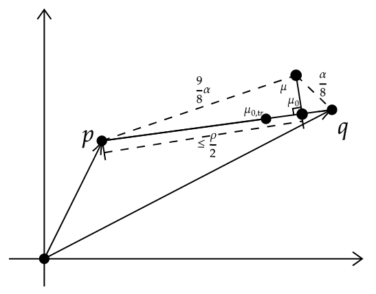
  Figure 1: $\left\|p-\mu\right\|_{2}>\frac{9\alpha}{8},\left\|q-\mu\right\|_{2}\leqslant\frac{\alpha}{8}$, and $\left\lvert p_{0}-\mu_{0}\right\rvert\leqslant\frac{\rho}{2}$.

• $\left\lvert p_{0}-\mu_{0}\right\rvert>\frac{\rho}{2}$. In this case, the triangle inequality implies that $\left\lvert p_{0}-q_{0}\right\rvert>\frac{\rho}{2}-\frac{\alpha}{8}\geqslant\frac{3\rho}{8}$, where the last inequality follows from the assumption $\alpha\leqslant\mathcal{O}\left(\frac{1}{m^{\frac{k-1}{k}}}\right)$. Now, we have to consider two cases depending on how $\left\lvert p_{0}-q_{0}\right\rvert$ compares with $\frac{17\rho}{16}$.

  When $\left\lvert p_{0}-\mu_{0}\right\rvert\leqslant\frac{17\rho}{16}$ (Figure 2), Lemma 5.1 implies $\left\lvert\mu_{0}-\mu_{0,\mathrm{tr}}\right\rvert\leqslant\frac{\rho}{8}$. Additionally, we have by Lemma 5.2 that $\left\lvert\bar{\mu}-\mu_{0,\mathrm{tr}}\right\rvert\leqslant\frac{\alpha}{16}$ with probability at least $1-\beta$. The triangle inequality yields that $\left\lvert q_{0}-\bar{\mu}\right\rvert\leqslant\frac{\alpha}{8}+\frac{\rho}{8}+\frac{\alpha}{16}=\frac{\rho}{8}+\frac{3\alpha}{16}\leqslant\frac{3\rho}{16}<\frac{\left\|p-q\right\|_{2}}{2}$. This immediately yields that $p$ loses the comparison to $q$.

  

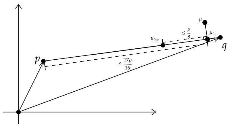
  Figure 2: $\left\lvert p_{0}-\mu_{0}\right\rvert>\frac{\rho}{2}$, and $\left\lvert p_{0}-\mu_{0}\right\rvert\leqslant\frac{17\rho}{16}$.

  When $\left\lvert p_{0}-\mu_{0}\right\rvert>\frac{17\rho}{16}$, we get that $\left\lvert p_{0}-\mu_{0,\mathrm{tr}}\right\rvert\in\left(\frac{15\rho}{16},\rho\right]$. We note that, by definition, we have $q_{0}>p_{0}$, so $q_{0}-p_{0}=\left\|q-p\right\|_{2}\geqslant\frac{3\rho}{8}$. Combining this with the fact that $\left\lvert q_{0}-\mu_{0}\right\rvert\leqslant\frac{\alpha}{8}$, we get that $\mu_{0}-p_{0}\geqslant\frac{3\rho}{8}-\frac{\alpha}{8}>0\implies\mu_{0}>p_{0}\implies\mu_{0,\mathrm{tr}}>p_{0}+\frac{15\rho}{16}$. By Lemma 5.2, we have that $\left\lvert\bar{\mu}-\mu_{0,\mathrm{tr}}\right\rvert\leqslant\frac{\alpha}{16}$ with probability at least $1-\beta$, implying that $\bar{\mu}>p_{0}+\frac{15}{16}\left(\rho-\alpha\right)$. If $\left\lvert q_{0}-\bar{\mu}\right\rvert\leqslant\frac{15}{16}\left(\rho-\alpha\right)$, then $q$ wins and $p$ loses. However, if that does not happen, we have to work differently.

  For the case where $\left\lvert q_{0}-\bar{\mu}\right\rvert\leqslant\frac{15}{16}\left(\rho-\alpha\right)$, let $q^{\prime}$ be any point that is at $\ell_{2}$-distance at most $\frac{\alpha}{8}$ from $\widetilde{\mu}=p+\frac{\rho}{2}\frac{\mu-p}{\left\|\mu-p\right\|_{2}}$ (Figure 3).

  

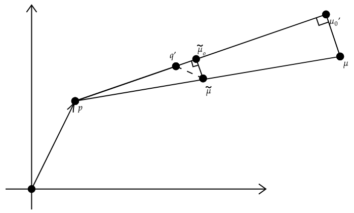
  Figure 3: $\left\lvert q_{0}-\bar{\mu}\right\rvert>\frac{15}{16}\left(\rho-\alpha\right)$.

  We project everything along the line that connects $p$ and $q^{\prime}$, so we get $p_{0}^{\prime}\coloneqq\left\langle\frac{q^{\prime}-p}{\left\|q^{\prime}-p\right\|_{2}},p\right\rangle,q_{0}^{\prime}\coloneqq\left\langle\frac{q^{\prime}-p}{\left\|q^{\prime}-p\right\|_{2}},q^{\prime}\right\rangle,\mu_{0}^{\prime}\coloneqq\left\langle\frac{q^{\prime}-p}{\left\|q^{\prime}-p\right\|_{2}},\mu\right\rangle$, and $\widetilde{\mu}_{0}\coloneqq\left\langle\frac{q^{\prime}-p}{\left\|q^{\prime}-p\right\|_{2}},\widetilde{\mu}\right\rangle$. By triangle inequality, we have $\left\lvert q^{\prime}_{0}-p^{\prime}_{0}\right\rvert=\left\|q^{\prime}-p\right\|_{2}\geqslant\left\|\widetilde{\mu}-p\right\|_{2}-\left\|q^{\prime}-\widetilde{\mu}\right\|_{2}\geqslant\frac{\rho}{2}-\frac{\alpha}{8}\geqslant\frac{3\rho}{8}$. Additionally, by triangle similarity, we have:

  $$\frac{\left\lvert\widetilde{\mu}_{0}-p_{0}^{\prime}\right\rvert}{\left\lvert\mu_{0}^{\prime}-p_{0}^{\prime}\right\rvert}=\frac{\left\|p-\widetilde{\mu}\right\|_{2}}{\left\|p-\mu\right\|_{2}}\iff\left\lvert\mu_{0}^{\prime}-p_{0}^{\prime}\right\rvert=\left\lvert\widetilde{\mu}_{0}-p_{0}^{\prime}\right\rvert\frac{\left\|p-\mu\right\|_{2}}{\left\|p-\widetilde{\mu}\right\|_{2}}=\left\lvert\widetilde{\mu}_{0}-p_{0}^{\prime}\right\rvert\frac{\left\lvert p_{0}-\mu_{0}\right\rvert}{\left\|p-\widetilde{\mu}\right\|_{2}},$$

  where, by the Pythagorean theorem $\left\lvert p_{0}^{\prime}-\widetilde{\mu}_{0}\right\rvert=\sqrt{\left\|p-\widetilde{\mu}\right\|_{2}^{2}-\left\|\widetilde{\mu}-\left(p+\widetilde{\mu}_{0}\frac{q^{\prime}-p}{\|q^{\prime}-p\|_{2}}\right)\right\|_{2}^{2}}\geqslant\sqrt{\left\|p-\widetilde{\mu}\right\|_{2}^{2}-\left\|\widetilde{\mu}-q^{\prime}\right\|_{2}^{2}}\geqslant\sqrt{\left\|p-\widetilde{\mu}\right\|_{2}^{2}-\left(\frac{\alpha}{8}\right)^{2}}$. As a result of all the previous, we get that $\left\lvert\mu_{0}^{\prime}-p_{0}^{\prime}\right\rvert$ is sufficiently large, so we can work similarly to the previous cases, but $p$ is guaranteed to lose this time.

∎

Assuming that $\left\|\mu\right\|_{\infty}\leqslant\alpha$, our goal is to use the above lemma to analyze the comparisons between a point $p$ with $\left\|p\right\|_{\infty}\leqslant\alpha$ and the elements of a local cover of the $\ell_{\infty}$-ball of radius $2\alpha$ that is centered around $p$. We will remove from the cover all the points that are at $\ell_{2}$-distance at most $\alpha$ from $p$. Our goal is to plug the above into the exponential mechanism in order to determine whether a point $p$ is close to the true mean of our distribution. For that reason, we will need to define a score function, which we do formally below:

Definition 5.5 ($\mathrm{Score}$ of a Point).

Let $X\coloneqq\left(X^{\left(1\right)},\dots,X^{\left(n\right)}\right)$ be a dataset consisting of $n$ batches $X^{\left(i\right)}\in\mathbb{R}^{m\times d},\forall i\in\left[d\right]$, and $p$ be a point in $\mathbb{R}^{d}$, and $\alpha>0$. We define $\mathrm{Score}_{X,D,\alpha}\left(p\right)$ of $p$ with respect to a domain $D\subset\mathbb{R}^{d}$ to be the minimum number of batches of $X$ that need to be changed to get a dataset $\overline{X}$ so that there exists $q\in D$, such that Algorithm 4 outputs False. If for all $q\in D\setminus\{p\}$ and all $X$, Algorithm 4 outputs True, then we define $\mathrm{Score}_{X,D,\alpha}\left(p\right)=n\alpha$. If the context is clear, we abbreviate the quantity to $\mathrm{Score}_{X}(p)$.

At this point, we recall the following lemma from [KSU20]:

Lemma 5.6.

The $\mathrm{Score}$ function satisfies the following:

$$\Delta_{\mathrm{Score},1}\leqslant 1.$$

We note that this lemma was established in the setting of item-level privacy, where the score is defined in terms of points that have to be changed for a point $p$ to lose a comparison, but the result still holds if instead of individual points we consider batches.

Algorithm 5 implements the above reasoning. The algorithm outputs a value that corresponds to the score of $p$, as defined in Definition 5.5. Its performance guarantees will be analyzed by using Lemmas 5.3 and 5.4.

Algorithm 5 Test Candidate

Input: A dataset $X\coloneqq\left(X^{\left(1\right)},\dots,X^{\left(n\right)}\right)\sim\left(\mathcal{D}^{\otimes m}\right)^{\otimes n}$, a point $p\in\mathbb{R}^{d}$, target error $\alpha$, target failure probability $\beta$.
      Output: $s\in\mathbb{N}$.

1:procedure $\mathrm{TestCan}_{p,\alpha,\beta}$($X$)

2:     for $i\in\left[d\right]$ do

3:         Let $J_{p,i}\coloneqq\left\{p_{i}-2\alpha,p_{i}-2\alpha+\frac{\alpha}{4\sqrt{d}},\dots,p_{i}+2\alpha-\frac{\alpha}{4\sqrt{d}},p_{i}+2\alpha\right\}$.

4:     end for

5:     Let $J_{p}\coloneqq\left(\bigotimes\limits_{i\in[d]}J_{p,i}\right)\setminus\left\{x\in\mathbb{R}^{d}\colon\left\|x-p\right\|_{2}\leqslant\alpha\right\}$.

6:     return $\mathrm{Score}_{X,J_{p},\alpha}\left(X\right)$.

7:end procedure

Lemma 5.7.

Let $\mathcal{D}$ be a distribution over $\mathbb{R}^{d}$ with mean $\left\|\mu\right\|_{\infty}\leqslant\alpha\leqslant\mathcal{O}\left(\frac{1}{m^{\frac{k-1}{k}}}\right)$, and $k$th moment bounded by $1$. Assume we are given $n\geqslant\mathcal{O}\left(\frac{d\log\left(\frac{d}{\beta}\right)}{m\alpha^{2}}\right)$ independently-drawn batches of size $m$, each denoted by $X^{(i)}\coloneqq\left(X^{(i)}_{1},\dots,X^{(i)}_{m}\right)\sim\mathcal{D}^{\otimes m},\forall i\in[n]$. For any $p\in\mathbb{R}^{d}$ such that $\left\|p\right\|_{\infty}\leqslant\alpha$, we have:

• If $\left\|p-\mu\right\|_{2}\leqslant\frac{\alpha}{8}$, we have for Algorithm 5 that, with probability at least $1-\beta$, it will output $\mathrm{Score}_{X,J_{p},\alpha}\left(X\right)\geqslant\Theta\left(\frac{n\alpha}{\rho}\right)$.

• If $\left\|p-\mu\right\|_{2}>\frac{9\alpha}{8}$, we have for Algorithm 5 that, with probability at least $1-\beta$, it will output $\mathrm{Score}_{X,J_{p},\alpha}\left(X\right)=0$.

Proof.

The proof follows almost immediately from Lemmas 5.3 and 5.4.

For the first case, the fact that Algorithm 5 constructs $J_{p}$ in a way that ensures that points $q$ considered are at least $\alpha$-far from $p$ suffices for us to be able to apply Lemma 5.3. Given that we want to apply the lemma for all points $q$, we need to set $\beta\to\frac{\beta}{\left(\Theta\left(\sqrt{d}\right)\right)^{d}}$. Indeed, by a union bound, the probability of getting the wrong result for at least one comparison is upper bounded by $\beta$, leading to the bound $n\geqslant\mathcal{O}\left(\frac{d\log\left(\frac{d}{\beta}\right)}{m\alpha^{2}}\right)$.

For the second case, we note that $J_{p}$ is an $\frac{\alpha}{8\sqrt{d}}$-cover with respect to the $\ell_{\infty}$-distance of the $\ell_{\infty}$-ball with radius $2\alpha$ that’s centered at $p$ (modulo the $\ell_{2}$-ball centered around $p$, which we’ve removed). We want to argue that there must exist a point $q\in J_{p}$ such that $\left\|q-\mu\right\|_{\infty}\leqslant\frac{\alpha}{8\sqrt{d}}$. This would follow immediately from the definition of $J_{p}$, had the points that lie at the $\ell_{2}$-ball of radius $\alpha$ that’s centered at $p$ not been removed. Thus, we need to argue that any point $q$ which satisfies $\left\|q-\mu\right\|_{\infty}\leqslant\frac{\alpha}{8\sqrt{d}}$ must also satisfy $\left\|p-q\right\|_{2}>\alpha$. We have that $\left\|q-\mu\right\|_{\infty}\leqslant\frac{\alpha}{8\sqrt{d}}\implies\left\|q-\mu\right\|_{2}\leqslant\frac{\alpha}{8}$. Since $\left\|p-\mu\right\|_{2}>\frac{9\alpha}{8}$, the triangle inequality yields that $\left\|p-q\right\|_{2}>\frac{9\alpha}{8}-\frac{\alpha}{8}=\alpha$, leading to the desired result. Additionally, the previous guarantee that the conditions of Lemma 5.4 are satisfied, and setting again $\beta\to\left(\Theta\left(\sqrt{d}\right)\right)^{d}$ completes the proof. ∎

We now have all the necessary tools to present the complete algorithm for fine estimation. Algorithm 6 constructs an $\ell_{\infty}$-cover of the set $\{x\in\mathbb{R}^{d}\colon\left\|x\right\|_{\infty}\leqslant\alpha\}$ that has granularity $\frac{2\alpha}{\sqrt{d}}$, and then calculates the score of all points of the cover and samples from the exponential mechanism.

Algorithm 6 Fine Estimation

Input: A dataset $X\coloneqq\left(X^{\left(1\right)},\dots,X^{\left(n\right)}\right)\sim\left(\mathcal{D}^{\otimes m}\right)^{\otimes n}$, target error $\alpha$, target failure probability $\beta$, privacy parameter $\varepsilon$.
      Output: $\widehat{\mu}\in\mathbb{R}^{d}$.

1:procedure $\mathrm{FineEst}_{\alpha,\beta,\varepsilon}$($X$)

2:     for $i\in\left[d\right]$ do

3:         Let $J_{i}\coloneqq\left\{-\alpha,-\alpha+\frac{2\alpha}{\sqrt{d}},\dots,\alpha-\frac{2\alpha}{\sqrt{d}},\alpha\right\}$.

4:     end for

5:     Let $J\coloneqq\bigotimes\limits_{i\in[d]}J_{i}$.

6:     for $p\in J$ do

7:         Run $\mathrm{TestCan}_{p,\frac{8\alpha}{9},\frac{\beta}{2\left(\Theta\left(\sqrt{d}\right)\right)^{d}}}(X)$ to calculate $\mathrm{Score}_{X,J_{p},\alpha}\left(X\right)$.

8:     end for

9:     Run the Exponential Mechanism with score function $\{\mathrm{Score}_{X,J_{p},\alpha}\left(X\right)\}_{p\in J}$ and privacy budget $\varepsilon$, to get a point $\widehat{\mu}$.

10:     return $\widehat{\mu}$.

11:end procedure

Lemma 5.8.

Let $\mathcal{D}$ be a distribution over $\mathbb{R}^{d}$ with mean $\left\|\mu\right\|_{\infty}\leqslant\alpha\leqslant\mathcal{O}\left(\frac{1}{m^{\frac{k-1}{k}}}\right)$, and $k$th moment bounded by $1$. Assume we are given $n\geqslant\mathcal{O}_{k}\left(\frac{d\log\left(\frac{d}{\beta}\right)}{m\alpha^{2}}+\frac{d\log\left(\frac{d}{\beta}\right)\sqrt{\log(m)}}{\sqrt{m}\alpha\varepsilon}+\frac{d\log\left(\frac{d}{\beta}\right)}{m\alpha^{\frac{k}{k-1}}\varepsilon}\right)$ independently-drawn batches of size $m$, each denoted by $X^{(i)}\coloneqq\left(X^{(i)}_{1},\dots,X^{(i)}_{m}\right)\sim\mathcal{D}^{\otimes m},\forall i\in[n]$. Then, for $\varepsilon,\beta>0$, there exists an $\varepsilon$-DP mechanism (Algorithm 6) which, given $\left(X^{(1)},\dots X^{(n)}\right)$ as input, outputs a point $\widehat{\mu}$ such that $\left\|\widehat{\mu}-\mu\right\|_{2}\leqslant\alpha$ with probability at least $1-\beta$.

Proof.

The privacy guarantee is an immediate consequence of the privacy guarantee of the exponential mechanism (Lemma 2.9), so we focus on the accuracy guarantee. By the definition of the set $J$, we have that there must exist a point $p\in J$ such that $\left\|p-\mu\right\|_{\infty}\leqslant\frac{\alpha}{\sqrt{d}}\implies\left\|p-\mu\right\|_{2}\leqslant\alpha$. Thus, what we must do is argue that, thanks to our choice of parameters, and the guarantees of the exponential mechanism imply that a point with $\left\|p-\mu\right\|_{2}\leqslant\alpha$ will be chosen with high probability. First, we note that Algorithm 6 uses Algorithm 5 with target error $\frac{8\alpha}{9}$, and probability $\frac{\beta}{2\left(\Theta\left(\sqrt{d}\right)\right)^{d}}$. Due to the number of batches $n$ that we have, as well as the guarantees of Lemma 5.7 we have that, for each point $p\in J$, except with probability $\frac{\beta}{2}$, the score of a point $p$ with $\left\|p-\mu\right\|_{2}\leqslant\frac{\alpha}{9}$ will be $\Theta\left(\frac{n\alpha}{\rho}\right)$, whereas the score of a point $p$ with $\left\|p-\mu\right\|_{2}>\alpha$ will be $0$. We have by Lemma 5.6 that the sensitivity of our score function is at most $1$. Thus, thanks to the guarantees of the exponential mechanism (Lemma 2.9), we have that, except with probability at least $\frac{\beta}{2}$, we have:

$$\mathrm{Score}(X,\widehat{\mu}) \geqslant\mathrm{OPT}_{\mathrm{Score}}(X)-\frac{2\Delta_{\mathrm{Score},1}}{\varepsilon}(\ln(|S|)+t)$$

$$\geqslant\Theta\left(\frac{n\alpha}{\rho}\right)-\frac{2}{\varepsilon}\left(\Theta\left(d\log(d)\right)+\log\left(\frac{2}{\beta}\right)\right)$$

$$\geqslant\Theta\left(\frac{n\alpha}{\sqrt{\frac{(k-1)\log m}{m}}+\frac{1}{m\alpha^{\frac{1}{k-1}}}}\right)-\frac{2}{\varepsilon}\left(\Theta\left(d\log(d)\right)+\log\left(\frac{2}{\beta}\right)\right)$$

We now need to consider two cases, depending on which term dominates in the denominator. If $\sqrt{\frac{(k-1)\log m}{m}}\leqslant\frac{1}{m\alpha^{\frac{1}{k-1}}}$, the previous can be lower-bounded by:

$$\Theta\left(n\alpha^{\frac{k}{k-1}}m\right)-\frac{2}{\varepsilon}\left(\Theta\left(d\log(d)\right)+\log\left(\frac{2}{\beta}\right)\right)$$

which, by assumption, is greater than $0$.

Conversely, if $\sqrt{\frac{(k-1)\log m}{m}}>\frac{1}{m\alpha^{\frac{1}{k-1}}}$, we get the lower bound:

$$\Theta\left(n\alpha\sqrt{\frac{m}{(k-1)\log(m)}}\right)-\frac{2}{\varepsilon}\left(\Theta\left(d\log(d)\right)+\log\left(\frac{2}{\beta}\right)\right),$$

which, by assumption again, is greater than $0$.

Thus, except with probability $\beta$, the exponential mechanism will output a point with score greater than $0$, implying that the point will be at distance at most $\alpha$ from the true mean. ∎

5.2 Coarse Estimation and the Full Algorithm

After focusing on fine estimation in the previous section, we can reason about coarse estimation, and tie everything together. Our coarse estimator is not a new algorithm: it consists of a component-wise application of the single-dimensional mean estimator that is implied by Theorem 3.14. In particular, given sufficiently many samples from a distribution with $k$th moment bounded by $1$ that has mean $\mu$, the estimator of Theorem 3.14 outputs a $\widehat{\mu}$ such that $|\widehat{\mu}-\mu|\leqslant\alpha$. Now, given samples from a distribution in $d$ dimensions with mean $\mu$ and $k$th moment bounded by $1$, we can apply this algorithm independelty for each coordinate, and obtain an estimate $\widehat{\mu}$ such that $\|\widehat{\mu}-\mu\|_{\infty}\leqslant\alpha$. This allows us to reduce to the case where $\|\mu\|_{\infty}\leqslant\alpha$, which was addressed in Section 5.1. Algorithm 7 presents the full pseudocode that handles both coarse and fine estimation.

Algorithm 7 Person-Level Pure-DP High-Dimensional Mean Estimation

Input: A dataset $X\coloneqq\left(X^{\left(1\right)},\dots,X^{\left(2n\right)}\right)\sim\left(\mathcal{D}^{\otimes m}\right)^{\otimes 2n}$, target error $\alpha$, target failure probability $\beta$, privacy parameter $\varepsilon$.
      Output: $\widehat{\mu}\in\mathbb{R}^{d}$.

1:procedure $\mathrm{PersonLevelMeanEst}_{\alpha,\beta,\varepsilon}$($X$)

2:     for $k\in\left[d\right]$ do

3:         Let $Y_{i}\coloneqq\left(\left(X^{(i)}_{1}\right)_{k},\dots,\left(X^{(i)}_{m}\right)_{k}\right)\in\mathbb{R}^{n},\forall i\in[n]$ be the batch consisting of the $k$-th component of each element of the $i$-th batch.

4:         Run the algorithm of Theorem 3.14 over $\left(Y_{1},\dots,Y_{n}\right)$ with target error $\alpha$, target failure probability $\frac{\beta}{2d}$, and privacy parameter $\frac{\varepsilon}{d}$, to obtain $\mu_{\mathtt{coarse},i}$.

5:     end for

6:     Let $\mu_{\mathtt{coarse}}\coloneqq\left(\mu_{\mathtt{coarse},1},\dots,\mu_{\mathtt{coarse},d}\right)$.

7:     for $i\in\{n+1,\dots,2n\}$ do

8:         Let $Z_{i-n}$ be the batch that is obtained by subtracting $\mu_{\mathtt{coarse}}$ from each element of $X^{(i)}$.

9:     end for

10:     Let $Z\coloneqq\left(Z_{1},\dots,Z_{n}\right)$

11:     Let $\widehat{\mu}\coloneqq\mathrm{FineEst}_{\alpha,\frac{\beta}{2},\varepsilon}(Z)+\mu_{\mathtt{coarse}}$.

12:     return $\widehat{\mu}$.

13:end procedure

Theorem 5.9.

Let $\mathcal{D}$ be a distribution over $\mathbb{R}^{d}$ with mean $\mu$, and $k$th moment bounded by $1$. Assume we are given $n\geqslant\mathcal{O}_{k}\left(\frac{d\log\left(d\right)}{m\alpha^{2}\beta}+\frac{d\log\left(\frac{d}{\beta}\right)\sqrt{\log(m)}}{\sqrt{m}\alpha\varepsilon}+\frac{d\log\left(\frac{d}{\beta}\right)}{m\alpha^{\frac{k}{k-1}}\varepsilon}+\frac{d\log\left(\frac{dRm}{\beta}\right)}{\varepsilon}\right)$ independently-drawn batches of size $m$, each denoted by $X^{(i)}\coloneqq\left(X^{(i)}_{1},\dots,X^{(i)}_{m}\right)\sim\mathcal{D}^{\otimes m},\forall i\in[n]$. Then, for $\varepsilon,\alpha,\beta>0$ with $\alpha\leqslant\mathcal{O}\left(\frac{1}{m^{\frac{k-1}{k}}}\right)$, there exists an $\varepsilon$-DP mechanism (Algorithm 6) which, given $\left(X^{(1)},\dots X^{(n)}\right)$ as input, outputs a point $\widehat{\mu}$ such that $\left\|\widehat{\mu}-\mu\right\|_{2}\leqslant\alpha$ with probability at least $1-\beta$.

Proof.

We start by establishing the privacy guarantee first. By the privacy guarantee of Theorem 3.14, and basic composition (Lemma 2.4), we get that we have $\varepsilon$-DP over the batches $(X^{(1)},\dots,X^{(n)})$. The guarantee is not affected when we later construct $\mu_{\mathtt{coarse}}$ and subtract it from the other datapoints, due to closure under post-processing (Lemma 2.3). By the privacy guarantee of Lemma 5.8, we are guaranteed $\varepsilon$-DP for the batches $X^{(n+1)},\dots X^{(2n)}$. The overall privacy guarantee then follows from parallel composition.

Now, it remains to establish the accuracy guarantee. By the guarantees of Theorem 3.14, we get that, except with probability $\frac{\beta}{2}$, we will have $\|\mu_{\mathtt{coarse}}-\mu\|_{\infty}\leqslant\alpha$. Thus, by the guarantees of Lemma 5.8, we get that, except with probability $\frac{\beta}{2}$, we will get a $\widehat{\mu}$ that satisfies $\left\|\widehat{\mu}-(\mu-\mu_{\mathtt{coarse}})\right\|_{2}=\left\|(\widehat{\mu}+\mu_{\mathtt{coarse}})-\mu\right\|_{2}\leqslant\alpha$. The desired accuracy guarantee follows directly from the last inequality and a union bound over failure events. ∎

6 Approximate-DP Lower Bounds for Bounded $k$h Moments

In this section, we establish lower bounds for private mean estimation of distributions with bounded $k$th moments in the person-level setting, under the constraint of $(\varepsilon,\delta)$-DP. Our bounds nearly match the upper bounds of Section 4. We start by stating the main theorem of the section.

Theorem 6.1.

Let $C_{1}>1$ be a sufficiently large absolute constant. Fix $k\geqslant 2$, and let $C(k)\coloneqq 2^{k}C^{(0)}(k)+1$, where $C^{(0)}(k)$ is a constant that is sufficiently large so that $\mathbb{E}\left[\left|\mathcal{N}(\mu,\sigma^{2})\right|^{k}\right]\leqslant C^{(0)}(k)\left(|\mu|+\sigma\right)^{k}$ is satisfied. Suppose $\alpha,\varepsilon\leqslant 1$, and $\delta\leqslant\min\left\{\widetilde{\Omega}\left(\frac{\alpha\varepsilon}{d}\right)^{C_{1}},\Omega\left(\min\left\{\frac{1}{n\sqrt{m}},\frac{\sqrt{d}}{n\sqrt{m}\sqrt{\log\left(\frac{n\sqrt{m}}{\sqrt{d}}\right)}}\right\}\right)\right\}$. Suppose that $M$ is an $(\varepsilon,\delta)$-DP mechanism that takes as input $X\coloneqq\left(X^{(1)},\dots,X^{(n)}\right)$ with $X^{(i)}\coloneqq\left(X^{(i)}_{1},\dots,X^{(i)}_{m}\right)\in\mathbb{R}^{m\times d},\forall i\in[n]$. Let $\mathcal{D}$ be any distribution over $\mathbb{R}^{d}$ such that $\mathbb{E}\left[\left|\left\langle\mathcal{D}-\mathbb{E}\left[\mathcal{D}\right],v\right\rangle\right|^{k}\right]\leqslant C(k),v\in\mathbb{S}^{d-1}$, and assume that $X^{(i)}_{j}\sim_{\text{i.i.d.}}\mathcal{D},\forall i\in[n],j\in[m]$. If, for any such $\mathcal{D}$, we have that $\mathbb{P}\left[\left\|M(X)-\mathbb{E}\left[\mathcal{D}\right]\right\|_{2}\leqslant\alpha\right]\geqslant\frac{2}{3}$, it must hold that $n\geqslant\widetilde{\Omega}\left(\frac{d}{m\alpha^{2}}+\frac{d}{\sqrt{m}\alpha\varepsilon}+\frac{d}{m\alpha^{k/{k-1}}\varepsilon}\right)$.

The proof of Theorem 6.1 can be split into two parts. The first part involves establishing the first and the last term of the sample complexity, whereas the second part focuses on the middle term. The former is significantly simpler since, as we will see, it comes as a direct consequence of a reduction from the item-level setting. In particular, we recall the following result from [Nar23]:

Proposition 6.2.

[Theorem $5.1$ from [Nar23]]. Let $C_{1}>1$ be a sufficiently large absolute constant. Fix $k\geqslant 2$, and let $C(k)\coloneqq 2^{k}C^{(0)}(k)+1$, where $C^{(0)}(k)$ is a constant that is sufficiently large so that $\mathbb{E}\left[\left|\mathcal{N}(\mu,\sigma^{2})\right|^{k}\right]\leqslant C^{(0)}(k)\left(|\mu|+\sigma\right)^{k}$ is satisfied. Suppose $\alpha,\varepsilon\leqslant 1$, and $\delta\leqslant\widetilde{\Omega}\left(\frac{\alpha\varepsilon}{d}\right)^{C_{1}}$. Suppose that $M$ is an $(\varepsilon,\delta)$-DP mechanism that takes as input $X\coloneqq\left(X_{1},\dots,X_{n}\right)$ with $X_{i}\in\mathbb{R}^{d},\forall i\in[n]$. Let $\mathcal{D}$ be any distribution over $\mathbb{R}^{d}$ such that $\mathbb{E}\left[\left|\left\langle\mathcal{D}-\mathbb{E}\left[\mathcal{D}\right],v\right\rangle\right|^{k}\right]\leqslant C(k),\forall v\in\mathbb{S}^{d-1}$, and assume that $X_{i}\sim_{\text{i.i.d.}}\mathcal{D},\forall i\in[n]$. If, for any such $\mathcal{D}$, we have that $\mathbb{P}\left[\left\|M(X)-\mathbb{E}\left[\mathcal{D}\right]\right\|_{2}\leqslant\alpha\right]\geqslant\frac{2}{3}$, it must hold that $n\geqslant\widetilde{\Omega}\left(\frac{d}{\alpha^{2}}+\frac{d}{\alpha^{\frac{k}{k-1}}\varepsilon}\right)$.

To understand why the above implies a lower bound for the batch setting, we need the following lemma. The lemma describes how, given oracle access to a mechanism for the person-level setting, we can construct a mechanism for the item-level setting. This allows us to reduce instances of the item-level problem to the person-level one. Hence, lower bounds on the number of items in the item-level setting imply lower bounds on the number of people in the person-level setting.

Lemma 6.3.

Let $\mathcal{D}$ be any distribution over $\mathbb{R}^{d}$. Let $\varepsilon,\delta,\alpha\geqslant 0$. Assume that any $(\varepsilon,\delta)$-DP mechanism $M\colon\mathbb{R}^{n^{\prime}\times d}\to\mathbb{R}^{d}$ which, given $X\coloneqq\left(X_{1},\dots,X_{n^{\prime}}\right)\sim\mathcal{D}^{\otimes n^{\prime}}$, outputs $M(X)$ such that $\mathbb{P}\left[\left\|M(X)-\mathbb{E}\left[\mathcal{D}\right]\right\|_{2}\leqslant\alpha\right]\geqslant\frac{2}{3}$ requires at least $n^{\prime}\geqslant n_{0}$ samples. Then, for any $(\varepsilon,\delta)$-DP mechanism $\bar{M}\colon\left(\mathbb{R^{m\times d}}\right)^{n}\to\mathbb{R}^{d}$ which, given $Y\coloneqq\left(Y^{(1)},\dots,Y^{(n)}\right)\sim\left(\mathcal{D}^{\otimes m}\right)^{\otimes n}$, outputs $\bar{M}(Y)$ such that $\mathbb{P}\left[\left\|M(Y)-\mathbb{E}[\mathcal{D}]\right\|_{2}\leqslant\alpha\right]\geqslant\frac{2}{3}$, it must hold that $n\geqslant\frac{n_{0}}{m}$.

Proof.

Let $\bar{M}$ be an $(\varepsilon,\delta)$-DP mechanism for the person-level setting that takes $n$ batches of size $m$ as input, and satisfies the desired accuracy guarantee. Given oracle access to this mechanism, we will show how to construct a mechanism $M$ for the item-level setting which shares the same accuracy guarantees. Assume that we have a dataset $X$ of size $n^{\prime}\coloneqq nm$ that has been drawn i.i.d. from $\mathcal{D}$. We partition the dataset into $n$ batches of size $m$. This results in a dataset $Y$ of size $n$, where each datapoint is an i.i.d. sample from $\mathcal{D}^{\otimes m}$. As a result, we can feed $Y$ into $\bar{M}$, and the resulting mechanism will be $M$. Then, $M$ inherits the accuracy and privacy guarantees of $\bar{M}$. Consequently, any lower bound on $n_{0}$ on $n^{\prime}$ also implies a lower bound on $n$, yielding the desired result. ∎

As a direct consequence of Proposition 6.2 and Lemma 6.3, we get the following corollary which accounts for two out of three terms that appear in the lower bound of Theorem 6.1.

Corollary 6.4.

Let $C_{1}>1$ be a sufficiently large absolute constant. Fix $k\geqslant 2$, and let $C(k)\coloneqq 2^{k}C^{(0)}(k)+1$, where $C^{(0)}(k)$ is a constant that is sufficiently large so that $\mathbb{E}\left[\left|\mathcal{N}(\mu,\sigma^{2})\right|^{k}\right]\leqslant C^{(0)}(k)\left(|\mu|+\sigma\right)^{k}$ is satisfied. Suppose $\alpha,\varepsilon\leqslant 1$, and $\delta\leqslant\widetilde{\Omega}\left(\frac{\alpha\varepsilon}{d}\right)^{C_{1}}$. Suppose that $M$ is an $(\varepsilon,\delta)$-DP mechanism that takes as input $X\coloneqq\left(X^{(1)},\dots,X^{(n)}\right)$ with $X^{(i)}\coloneqq\left(X^{(i)}_{1},\dots,X^{(i)}_{m}\right)\in\mathbb{R}^{m\times d},\forall i\in[n]$. Let $\mathcal{D}$ be any distribution over $\mathbb{R}^{d}$ such that $\mathbb{E}\left[\left|\left\langle\mathcal{D}-\mathbb{E}\left[\mathcal{D}\right],v\right\rangle\right|^{k}\right]\leqslant C(k),v\in\mathbb{S}^{d-1}$, and assume that $X^{(i)}_{j}\sim_{\text{i.i.d.}}\mathcal{D},\forall i\in[n],j\in[m]$. If, for any such $\mathcal{D}$, we have that $\mathbb{P}\left[\left\|M(X)-\mathbb{E}\left[\mathcal{D}\right]\right\|_{2}\leqslant\alpha\right]\geqslant\frac{2}{3}$, it must hold that $n\geqslant\widetilde{\Omega}\left(\frac{d}{m\alpha^{2}}+\frac{d}{m\alpha^{\frac{k}{k-1}}\varepsilon}\right)$.

It remains to argue about the term $\frac{d}{\sqrt{m}\alpha\varepsilon}$ that appears in Theorem 6.1. To do so, we need to invoke a result that is implicit in [LSA⁺21]. Theorem $6$ in that work is concerned with proving a lower bound on the rates of Stochastic Convex Optimization with person-level privacy. Establishing the result involves reducing from Gaussian mean estimation under person-level privacy, for which [LSA⁺21] proves a lower bound in Appendix E.2. We explicitly state the result here.

Proposition 6.5.

Given $X\sim\left(\mathcal{N}(\mu,\mathbb{I})^{\otimes m}\right)^{\otimes n}$ with $\mu\in[\pm 1]^{d}$, for any $\alpha=\mathcal{O}(\sqrt{d})$ and any $(\varepsilon,\delta)$-DP mechanism $M\colon\left(\mathbb{R}^{m\times d}\right)^{n}\to[\pm 1]^{d}$ with $\varepsilon,\delta\in[0,1]$, and $\delta\leqslant\Omega\left(\min\left\{\frac{1}{n\sqrt{m}},\frac{\sqrt{d}}{n\sqrt{m}\sqrt{\log\left(\frac{n\sqrt{m}}{\sqrt{d}}\right)}}\right\}\right)$ that satisfies $\underset{X,M}{\mathbb{E}}\left[\left\|M(X)-\mu\right\|_{2}^{2}\right]\leqslant\alpha^{2}$, it holds that $n=\Omega\left(\frac{d}{\sqrt{m}\alpha\varepsilon}\right)$.

Theorem 6.1 follows directly by combining Corollary 6.4 and Proposition 6.5.

Appendix A Extra proofs for Section 4

A.1 Missing Proofs from Section 4.1.1

Lemma A.1.

Let $m,j$ be integers satisfying $1\leqslant j\leqslant m$. It follows that

$$\binom{m}{j}\leqslant\left(\frac{em}{j}\right)^{j}.$$

Lemma A.2.

Let $a>0$ and $b\geqslant 0$ be constants. The function $(ax^{b})^{x}$ defined on $x>0$ is convex.

Proof.

Note that

$$\frac{d^{2}}{dx^{2}}(ax^{b})^{x}=(ax^{b})^{x}\left(\left(\ln(ax^{b})+b\right)^{2}+\frac{b}{x}\right)\geqslant 0$$

when $a,x>0$, $b\geqslant 0$, completing the proof. ∎

For the next lemma, recall that the function $f(\ell)$ is defined as

$$f(\ell)=\Theta\left(\frac{d^{k/2}\cdot 2^{\ell(k-1)}\log^{k}m}{m^{k-1}t^{k}}\right)^{2^{\ell-1}}.$$

See 4.1.1

Proof.

Set $x=2^{\ell}$, $a=\frac{m^{1/2}d^{k/4}\log^{k/2}m}{m^{k/2}t^{k/2}}$, and $b=\frac{k-1}{2}$. Observe that $a,b,x>0$. Thus,

$$f(\ell) =\left(\frac{md^{k/2}2^{\ell(k-1)}\log^{k}m}{m^{k}t^{k}}\right)^{2^{\ell-1}}$$

$$=\left(\frac{m^{1/2}d^{k/4}\log^{k/2}m}{m^{k/2}t^{k/2}}\cdot 2^{\ell\left(\frac{k-1}{2}\right)}\right)^{2^{\ell}}$$

$$=(ax^{b})^{x},$$

which we know by Lemma A.2 is convex with respect to $x>0$, and thus is convex with respect to $\ell$. ∎

A.2 Missing Proofs from Section 4.1.2

Lemma A.3.

Let $k>2$ and $t>0$. Let $X_{i}$ be a random vector in $\mathbb{R}^{d}$ with $\operatorname*{\mathbb{E}}[X_{i}]=0$ and $k$-th moment bounded by $1$. Let $r_{1}=\frac{d}{t}$. Let $Y_{i}=X_{i}\cdot\mathbb{I}\left[\lVert X_{i}\rVert_{2}<r_{1}\right]$. There exists $t_{2}=\Omega(\sqrt{d})$ such that, for all positive $t\leqslant t_{2}$,

$$\lVert\operatorname*{\mathbb{E}}\left[Y_{i}\right]\rVert_{2}\leqslant\min\left(\frac{t}{6},\frac{d}{t}\right).$$

Proof of Lemma A.3.

Since $\operatorname*{\mathbb{E}}[X_{i}]=0$, we have that

$$\operatorname*{\mathbb{E}}[X_{i}]=\operatorname*{\mathbb{E}}\left[X_{i}\cdot\mathbb{I}\left[\lVert X_{i}\rVert_{2}<r_{1}\right]\right]+\operatorname*{\mathbb{E}}\left[X_{i}\cdot\mathbb{I}\left[\lVert X_{i}\rVert_{2}\geqslant r_{1}\right]\right]$$

which implies that

$$\lVert\operatorname*{\mathbb{E}}\left[Y_{i}\right]\rVert_{2} =\lVert\operatorname*{\mathbb{E}}\left[X_{i}\cdot\mathbb{I}\left[\lVert X_{i}\rVert_{2}<r_{1}\right]\right]\rVert_{2}$$

$$=\lVert\operatorname*{\mathbb{E}}[X_{i}]-\operatorname*{\mathbb{E}}\left[X_{i}\cdot\mathbb{I}\left[\lVert X_{i}\rVert_{2}\geqslant r_{1}\right]\right]\rVert_{2}$$

$$=\lVert\operatorname*{\mathbb{E}}\left[X_{i}\cdot\mathbb{I}\left[\lVert X_{i}\rVert_{2}\geqslant r_{1}\right]\right]\rVert_{2}$$

So now,

$$\lVert\operatorname*{\mathbb{E}}\left[X_{i}\cdot\mathbb{I}\left[\lVert X_{i}\rVert_{2}\geqslant r_{1}\right]\right]\rVert_{2}$$

$$\leqslant\operatorname*{\mathbb{E}}\left[\lVert X_{i}\rVert_{2}\cdot\mathbb{I}\left[\lVert X_{i}\rVert_{2}\geqslant r_{1}\right]\right]$$

$$=\int_{x=0}^{\infty}\operatorname*{\mathbb{P}}\left[\lVert X_{i}\rVert_{2}\cdot\mathbb{I}\left[\lVert X_{i}\rVert_{2}\geqslant r_{1}\right]>x\right]\,\mathrm{d}x$$

$$=\int_{x=0}^{r_{1}}\operatorname*{\mathbb{P}}\left[\lVert X_{i}\rVert_{2}\cdot\mathbb{I}\left[\lVert X_{i}\rVert_{2}\geqslant r_{1}\right]>x\right]\,\mathrm{d}x$$

$$\phantom{oooooo}+\int_{x=r_{1}}^{\infty}\operatorname*{\mathbb{P}}\left[\lVert X_{i}\rVert_{2}\cdot\mathbb{I}\left[\lVert X_{i}\rVert_{2}\geqslant r_{1}\right]>x\right]\,\mathrm{d}x$$

$$=\int_{x=0}^{r_{1}}\operatorname*{\mathbb{P}}\left[\lVert X_{i}\rVert_{2}\geqslant r_{1}\right]\,\mathrm{d}x+\int_{x=r_{1}}^{\infty}\operatorname*{\mathbb{P}}\left[\lVert X_{i}\rVert_{2}>x\right]\,\mathrm{d}x$$

$$=\int_{x=0}^{r_{1}}\left(\frac{d^{1/2}}{r_{1}}\right)^{k}\,\mathrm{d}x+\int_{x=r_{1}}^{\infty}\left(\frac{d^{1/2}}{x}\right)^{k}\,\mathrm{d}x$$ (by Lemma 4.7)

$$=\frac{d^{k/2}}{r_{1}^{k-1}}+\frac{d^{k/2}}{r_{1}^{k-1}(k-1)}$$

$$\leqslant\frac{2d^{k/2}}{r_{1}^{k-1}} k\geqslant 2$$ (since )

$$=\frac{2t^{k-1}}{d^{k/2-1}}.$$

To finish the proof, note that

$$\frac{2t^{k-1}}{d^{k/2-1}}\leqslant 2t\left(\frac{t}{\sqrt{d}}\right)^{k-2}\leqslant\frac{t}{6},$$

which uses the assumption that $t\leqslant t_{2}$ for some $t_{2}\leqslant 12^{\frac{-1}{k-2}}\sqrt{d}$. Also note that

$$\frac{2t^{k-1}}{d^{k/2-1}}\leqslant\frac{2t^{k}}{d^{k/2}}\cdot\frac{d}{t}\leqslant\frac{d}{t}$$

which uses the assumption that $t\leqslant t_{2}$ for some $t_{2}\leqslant 2^{-1/k}\sqrt{d}$. ∎

Lemma A.4.

Let $k>2$ and $t>0$. Let $X_{i}$ be a random vector in $\mathbb{R}^{d}$ with $\operatorname*{\mathbb{E}}[X_{i}]=0$ and $k$-th moment bounded by $1$. Let $r_{1}=\frac{d}{t}$. Let $Y_{i}=X_{i}\cdot\mathbb{I}\left[\lVert X_{i}\rVert_{2}<r_{1}\right]$. Let $Z_{i}=Y_{i}-\operatorname*{\mathbb{E}}\left[Y_{i}\right]$. There exists $t_{2}=\Omega(\sqrt{d})$ such that, for all positive $t\leqslant t_{2}$,

$$\operatorname*{\mathbb{E}}[Z_{i}] =0,$$ (27)

$$\operatorname*{\mathbb{E}}\left[\lVert Z_{i}\rVert^{2}_{2}\right] \leqslant d\text{, and}$$ (28)

$$\lVert Z_{i}\rVert_{2} \leqslant 2r_{1}.$$ (29)

Proof.

Note that (27) is satisfied by design of the $Z_{i}$’s. We now show that (28) holds. Note that

$$\operatorname*{\mathbb{E}}\left[\lVert Z_{i}\rVert^{2}_{2}\right]=\operatorname*{\mathbb{E}}\left[\lVert Y_{i}-\operatorname*{\mathbb{E}}\left[Y_{i}\right]\rVert^{2}_{2}\right]\leqslant\operatorname*{\mathbb{E}}\left[\lVert Y_{i}\rVert^{2}_{2}\right]\leqslant\operatorname*{\mathbb{E}}\left[\lVert X_{i}\rVert^{2}_{2}\right],$$

where the first inequality above comes from the fact that setting $y=\operatorname*{\mathbb{E}}\left[Y_{i}\right]$ minimizes $\operatorname*{\mathbb{E}}\left[\lVert Y_{i}-y\rVert^{2}_{2}\right]$. Observe that

$$\operatorname*{\mathbb{E}}\left[\lVert X_{i}\rVert_{2}^{2}\right]=\operatorname*{\mathbb{E}}\left[\sum_{j=1}^{d}\langle X_{i},e_{j}\rangle^{2}\right]=\sum_{j=1}^{d}\operatorname*{\mathbb{E}}\left[\langle X_{i},e_{j}\rangle^{2}\right]\leqslant\sum_{j=1}^{d}\operatorname*{\mathbb{E}}\left[\langle X_{i},e_{j}\rangle^{k}\right]\leqslant d,$$ (30)

where the last inequality comes from the assumption that, for every $u$ with $\lVert u\rVert_{2}=1$, $\operatorname*{\mathbb{E}}\left[\langle X_{i},u\rangle^{k}\right]\leqslant 1$. Thus, $\operatorname*{\mathbb{E}}\left[\lVert Z_{i}\rVert^{2}_{2}\right]\leqslant d$ and so (28) is satisfied.

Now we show that the last constraint, (29), also holds. We start by expanding $\lVert Z_{i}\rVert_{2}$ for some $i$.

$$\lVert Z_{i}\rVert_{2} =\lVert X_{i}\cdot\mathbb{I}\left[\lVert X_{i}\rVert_{2}<r_{1}\right]-\operatorname*{\mathbb{E}}\left[Y_{i}\right]\rVert_{2}$$

$$\leqslant\lVert X_{i}\cdot\mathbb{I}\left[\lVert X_{i}\rVert_{2}<r_{1}\right]\rVert_{2}+\lVert\operatorname*{\mathbb{E}}\left[Y_{i}\right]\rVert_{2}$$

$$\leqslant r_{1}+\lVert\operatorname*{\mathbb{E}}\left[Y_{i}\right]\rVert_{2}$$

$$\leqslant 2r_{1}.$$ (by Lemma A.3)

∎

Lemma A.5.

Let $k>2$ and $t>0$. Let $X_{i}$ be a random vector in $\mathbb{R}^{d}$ with $\operatorname*{\mathbb{E}}[X_{i}]=0$ and $k$-th moment bounded by $1$. Let $r_{1}=\frac{d}{t}$. Let $Y_{i}=X_{i}\cdot\mathbb{I}\left[\lVert X_{i}\rVert_{2}<r_{1}\right]$. Let $Z_{i}=Y_{i}-\operatorname*{\mathbb{E}}\left[Y_{i}\right]$. There exists $t_{2}=\Omega(\sqrt{d})$ such that, for all positive $t\leqslant t_{2}$,

$$\operatorname*{\mathbb{P}}\left[\Big{\lVert}\sum_{i=1}^{m}Z_{i}\Big{\rVert}_{2}\geqslant m\left(\frac{t}{3}-\lVert\operatorname*{\mathbb{E}}\left[Y_{i}\right]\rVert_{2}\right)\right]\leqslant\exp\left(-\Theta\left(\frac{mt^{2}}{d}\right)\right)$$

Proof.

We apply the Vectorized Bernstein’s Inequality (i.e. Lemma 4.13) by setting $t^{\prime}=t/3-\lVert\operatorname*{\mathbb{E}}\left[Y_{i}\right]\rVert_{2}$, $r=2r_{1}$, and $\sigma^{2}=d$. One can check using Lemma A.3 that $0<t^{\prime}<\sigma^{2}/r$ is satisfied for all $0<t<\sqrt{d}/12$. Thus,

$$\operatorname*{\mathbb{P}}\left[\Big{\lVert}\sum_{i=1}^{m}Z_{i}\Big{\rVert}_{2}\geqslant m(t/3-\lVert\operatorname*{\mathbb{E}}\left[Y_{i}\right]\rVert_{2})\right] =\operatorname*{\mathbb{P}}\left[\Big{\lVert}\sum_{i=1}^{m}Z_{i}\Big{\rVert}_{2}\geqslant mt^{\prime}\right]$$

$$\leqslant\exp\left(-m\frac{(t^{\prime})^{2}}{8\sigma^{2}}+\frac{1}{4}\right)$$ (by Lemma 4.13)

$$=\exp\left(-m\frac{(t/3-\lVert\operatorname*{\mathbb{E}}\left[Y_{i}\right]\rVert_{2})^{2}}{8d}+\frac{1}{4}\right)$$

$$\leqslant\exp\left(-m\frac{(t/3-t/6)^{2}}{8d}+\frac{1}{4}\right)$$ (by Lemma A.3)

$$\leqslant\exp\left(-\Theta\left(\frac{mt^{2}}{d}\right)\right).$$

∎

For the next lemma, recall that the function $f(\ell)$ is defined as

$$f(\ell)=\Theta\left(\frac{d^{k/2}\cdot 2^{\ell(k-1)}\log^{k}m}{m^{k-1}t^{k}}\right)^{2^{\ell-1}}.$$

Lemma A.6.

Let $m,d,t>0$ and $k>2$. Let $r_{2}=mt/(3\log m)$ and let $r_{1}=d/t$. There exists $t_{1}=O\left(\sqrt{\frac{d\log m}{m}}\right)$ and $t_{2}=\Omega\left(\sqrt{d}\log^{\frac{-1}{k-2}}m\right)$ such that, for all $t\in[t_{1},t_{2}]$,

$$f(\log(r_{2}/r_{1}))=\tilde{O}\left(\frac{d^{k/2}}{m^{k-1}t^{k}}\right).$$

Proof.

Define $g(t)=f\left(\log\left(\frac{mt^{2}}{3d\log m}\right)\right)$. Note that

$$\min_{t\in[t_{1},t_{2}]}\tilde{O}\left(\frac{d^{k/2}}{m^{k-1}t^{k}}\right)=\tilde{O}\left(\frac{1}{m^{k-1}}\right).$$

Thus, it suffices to show that

$$\max_{t\in[t_{1},t_{2}]}g(t)\leqslant\tilde{O}\left(\frac{1}{m^{k-1}}\right).$$ (31)

We break the proof into two parts. First, we show that

$$\max_{t\in[t_{1},t_{2}]}g(t)\in\{g(t_{1}),g(t_{2})\}.$$ (32)

Second, we show that

$$g(t_{1}),g(t_{2})\leqslant\tilde{O}\left(\frac{1}{m^{k-1}}\right).$$ (33)

To show (32), it suffices to show that $g(t)$ is convex with respect to $t$ for $t>0$. Note that

$$g(t) =\Theta\left(\frac{md^{k/2}\left(\frac{mt^{2}}{3d\log m}\right)^{k-1}\log^{k}m}{m^{k}t^{k}}\right)^{\frac{mt^{2}}{6d\log m}}$$

$$=\Theta\left(\frac{d^{-k/2+1}t^{k-2}\log m}{3^{k-1}}\right)^{\frac{mt^{2}}{6d\log m}}$$

$$=\Theta\left(\log m\left(\frac{t^{2}}{d}\right)^{\frac{k-2}{2}}\right)^{\frac{mt^{2}}{6d\log m}}.$$

Note that

$$\Theta\left(\log m\left(\frac{t^{2}}{d}\right)^{\frac{k-2}{2}}\right)^{\frac{mt^{2}}{6d\log m}}=\left(\left(\frac{\log m}{d^{\frac{k-2}{2}}}\right)^{\frac{m}{6d\log m}}\left(t^{2}\right)^{\frac{k-2}{2}\cdot\frac{m}{6d\log m}}\right)^{t^{2}}=(ax^{b})^{x},$$

for $x=t^{2}$, $a=\left(\frac{\log m}{d^{\frac{k-2}{2}}}\right)^{\frac{m}{6d\log m}}$ and $b=\frac{k-2}{2}\cdot\frac{m}{6d\log m}$. Since $a,b,x>0$, then by Lemma A.2, $(ax^{b})^{x}$ is convex with respect to $x$, and so $g$ is also convex for $t>0$. Thus, (32) holds.

We move on to showing (33). Let $t_{1}=\sqrt{\frac{cd\log m}{m}}$ for some $c\geqslant\frac{12(k-1)}{k-2}$. When $t=t_{1}$,

$$g(t_{1}) =\Theta\left(\log m\left(\frac{t_{1}^{2}}{d}\right)^{\frac{k-2}{2}}\right)^{\frac{mt_{1}^{2}}{6d\log m}}$$

$$=\Theta\left(\log m\left(\frac{\log m}{m}\right)^{\frac{k-2}{2}}\right)^{\frac{c}{6}}$$

$$=\tilde{O}\left(\frac{1}{m^{\left(\frac{k-2}{2}\cdot\frac{c}{6}\right)}}\right)$$

$$=\tilde{O}\left(\frac{1}{m^{k-1}}\right).$$

Let $t_{2}=\frac{\sqrt{d}\log^{\frac{-1}{k-2}}m}{2}$. When $t=t_{2}$,

$$g(t_{2}) =\Theta\left(\log m\left(\frac{t_{2}^{2}}{d}\right)^{\frac{k-2}{2}}\right)^{\frac{mt_{2}^{2}}{6d\log m}}$$

$$=O\left(\frac{1}{2}\right)^{O(m)}$$

$$=\tilde{O}\left(\frac{1}{m^{k-1}}\right).$$

∎

A.3 Missing Proofs from Section 4.1.4

Lemma A.7.

Let $\ell>0$. Let $\lVert u-\mu\rVert_{2}<\rho$. It follows that

$$\lVert X-\mu\rVert_{2}\geqslant\lVert X-\mathrm{clip}_{\rho,u}\left(X\right)\rVert_{2}+\rho-\lVert\mu-u\rVert_{2}.$$

Proof.

Let $r=\lVert u-\mu\rVert_{2}$, and let $\mathbb{B}^{d}(u,r)$ be the $\ell_{2}$ ball in $d$ dimensions of radius $r$ that is centered at $u$. Note that, by assumption, $r<\rho$, and so it follows that $\mu\in\mathbb{B}^{d}(u,r)\subseteq\mathbb{B}^{d}(u,\rho)$. Let

$$\mu^{*}=\operatorname*{arg\,min}_{\mu^{\prime}\in\mathbb{B}^{d}(u,r)}\lVert X-\mu^{\prime}\rVert_{2}.$$

One can check that $\mu^{*}$ is a point on the surface of $\mathbb{B}^{d}(u,r)$, and also that $u$, $\mu^{*}$, $\mathrm{clip}_{\rho,u}\left(X\right)$, and $X$ are collinear and arranged sequentially on the line in that order. We use these facts to relate the quantities $\lVert X-\mu\rVert_{2}$ and $\lVert X-\mathrm{clip}_{\rho,u}\left(X\right)\rVert_{2}$:

$$\lVert X-\mu\rVert_{2} \geqslant\lVert X-\mu^{*}\rVert_{2}$$

$$=\lVert X-u\rVert_{2}-\lVert\mu^{*}-u\rVert_{2}$$

$$=\lVert X-\mathrm{clip}_{\rho,u}\left(X\right)\rVert_{2}+\lVert\mathrm{clip}_{\rho,u}\left(X\right)-u\rVert_{2}-\lVert\mu^{*}-u\rVert_{2}$$

$$\geqslant\lVert X-\mathrm{clip}_{\rho,u}\left(X\right)\rVert_{2}+\rho-\lVert\mu-u\rVert_{2}$$ (34)

Note that $\lVert X-\mathrm{clip}_{\rho,u}\left(X\right)\rVert_{2}\geqslant\ell$ thus implies $\lVert X-\mu\rVert_{2}\geqslant\ell+\rho-\lVert\mu-u\rVert_{2}$, completing the proof. ∎

A.4 Missing Proofs from Section 4.4

See 4.21

Proof.

Let $Y^{(i)}=\frac{1}{m}\sum_{j=1}^{m}X^{(1)}_{j}\in\mathbb{R}^{d}$, and let $Y^{(i)}(\ell)\in\mathbb{R}$ be the $\ell$th coordinate of $Y^{(i)}$. We begin by expanding the following expression of expectation:

$$\operatorname*{\mathbb{E}}\left[\left\lVert\frac{1}{n}\sum_{i=1}^{n}S_{i}-\operatorname*{\mathbb{E}}\left[\frac{1}{n}\sum_{i=1}^{n}S_{i}\right]\right\rVert_{2}^{2}\right]$$

$$=\frac{1}{n^{2}}\operatorname*{\mathbb{E}}\left[\left\lVert\sum_{i=1}^{n}(S_{i}-\operatorname*{\mathbb{E}}\left[S_{i}\right])\right\rVert_{2}^{2}\right]$$

$$\leqslant\frac{1}{n^{2}}\operatorname*{\mathbb{E}}\left[\sum_{i=1}^{n}\left\lVert S_{i}-\operatorname*{\mathbb{E}}\left[S_{i}\right]\right\rVert_{2}^{2}\right]$$

$$=\frac{1}{n}\operatorname*{\mathbb{E}}\left[\left\lVert S_{1}-\operatorname*{\mathbb{E}}\left[S_{1}\right]\right\rVert_{2}^{2}\right]$$

$$\leqslant\frac{1}{n}\operatorname*{\mathbb{E}}\left[\left\lVert\frac{1}{m}\sum_{j=1}^{m}X_{j}^{(1)}-\operatorname*{\mathbb{E}}\left[\frac{1}{m}\sum_{j=1}^{m}X_{j}^{(1)}\right]\right\rVert_{2}^{2}\right]$$

$$=\frac{1}{n}\operatorname*{\mathbb{E}}\left[\sum_{\ell=1}^{d}\left(Y^{(1)}(\ell)-\operatorname*{\mathbb{E}}\left[Y^{(1)}(\ell)\right]\right)^{2}\right]$$

$$\leqslant\frac{d}{nm}.$$

By Chebyshev’s Inequality,

$$\operatorname*{\mathbb{P}}\left[\left\lVert\frac{1}{n}\sum_{i=1}^{n}S_{i}-\operatorname*{\mathbb{E}}\left[\frac{1}{n}\sum_{i=1}^{n}S_{i}\right]\right\rVert_{2}\geqslant\alpha\right]=O\left(\frac{d}{mn\alpha^{2}}\right)\leqslant\beta.$$

∎

Lemma A.8.

Assume the setting in Lemma 4.22. It follows that $T_{1},T_{3}\leqslant\frac{\rho_{2}}{8\sqrt{d}}$.

Proof.

Recall that

$$\rho_{1}=\max\left(\sqrt{\frac{d}{m}},\frac{n^{1/k}\varepsilon^{1/k}d^{\frac{1}{2}-\frac{1}{2k}}}{(\log 1/\delta)^{1/(2k)}m^{1-1/k}}\right).$$ (35)

Note that the second term in the maximum of (35) is that which balances $T_{1}$ and $T_{3}$, up to polylogarithmic factors. Thus, when $\rho_{1}$ is set to this term,

$$\left\lVert\mu-\operatorname*{\mathbb{E}}\left[\mathrm{clip}_{\rho,u}\left(X\right)\right]\right\rVert_{2}+\left\lVert W_{1}\right\rVert_{2} =\tilde{O}\left(\left\lVert W_{1}\right\rVert_{2}\right)$$

$$=\tilde{O}\left(\frac{\rho_{1}\sqrt{d\log 1/\delta}}{n\varepsilon}\right)$$

$$=\frac{\rho_{1}}{8d^{\frac{1}{2}}d^{\frac{1}{2k}}} n$$ (by assumption on )

$$\leqslant\frac{\rho_{2}}{8\sqrt{d}},$$

where the last inequality comes from the fact that $\rho_{1}/\rho_{2}\leqslant d^{1/2k}$. When the first term in the maximum of (35) dominates, one can observe that $T_{1}$ dominates $T_{3}$ asymptotically, up to polylogarithmic factors. Also note that $\rho_{1}=\sqrt{d/m}$ implies $\rho_{2}=\sqrt{d/m}$. Thus, when $\rho_{1}$ is set to this term,

$$\left\lVert\mu-\operatorname*{\mathbb{E}}\left[\mathrm{clip}_{\rho,u}\left(X\right)\right]\right\rVert_{2}+\left\lVert W_{1}\right\rVert_{2} =\tilde{O}\left(\lVert W_{1}\rVert_{2}\right)$$

$$=\tilde{O}\left(\frac{d\sqrt{\log 1/\delta}}{\sqrt{m}n\varepsilon}\right) \rho_{1}=\sqrt{d/m}$$ (since )

$$=\frac{1}{8\sqrt{m}} n$$ (by assumption on )

$$=\frac{\rho_{1}}{8\sqrt{d}}$$

$$=\frac{\rho_{2}}{8\sqrt{d}}.$$

∎

See 4.23

Proof.

Recall that $u_{2}$ is the output of an application of Algorithm 2. Define $\mathsf{V}_{i}\coloneqq\mathrm{clip}_{\rho,u}\left(\frac{1}{m}\sum_{j=1}^{m}V_{j}^{(i)}\right)$ and define $W_{2}$ such that

$$W_{2}\sim\mathcal{N}\left(0,\left(\frac{8\sqrt{d}\rho_{2}\sqrt{2\ln(16/\delta)}}{n\varepsilon}\right)^{2}\cdot\mathbb{I}_{d\times d}\right).$$

We begin by expanding $\lVert\hat{\mu}-\mu\rVert_{2}$:

$$\lVert\hat{\mu}-\mu\rVert_{2} =\left\lVert W_{2}+\frac{1}{n}\sum_{i=1}^{n}\mathsf{V}_{i}-\operatorname*{\mathbb{E}}\left[\mathsf{V_{1}}\right]+\operatorname*{\mathbb{E}}\left[\mathsf{V_{1}}\right]-\mu\right\rVert_{2}$$

$$\leqslant\underbrace{\lVert W_{2}\rVert_{2}}_{T_{1}\coloneqq}+\underbrace{\left\lVert\frac{1}{n}\sum_{i=1}^{n}\mathsf{V}_{i}-\operatorname*{\mathbb{E}}\left[\mathsf{V_{1}}\right]\right\rVert_{2}}_{T_{2}\coloneqq}+\underbrace{\left\lVert\operatorname*{\mathbb{E}}\left[\mathsf{V_{1}}\right]-\mu\right\rVert_{2}}_{T_{3}\coloneqq}.$$

By assumption on $n$, we can apply Lemma 4.21 which says that, with probability at least $0.95$,

$$T_{2}=\left\lVert\frac{1}{n}\sum_{i=1}^{n}\mathsf{V}_{i}-\operatorname*{\mathbb{E}}\left[\mathsf{V_{1}}\right]\right\rVert_{2}\leqslant\frac{\alpha}{2}.$$

By the properties of Gaussian random variables, it follows that with probability at least $0.95$,

$$T_{1}=\left\lVert W_{2}\right\rVert_{2}=O\left(\frac{\rho_{2}\sqrt{d\log 1/\delta}}{n\varepsilon}\right).$$

When $\rho_{2}=\sqrt{d/m}$,

$$T_{1}=O\left(\frac{d\sqrt{\log(1/\delta)}}{\sqrt{m}n\varepsilon}\right)\leqslant\frac{\alpha}{4},$$ (36)

by assumption on $n$ and $n_{0}$. Likewise, when $\rho_{2}=\frac{n^{1/k}\varepsilon^{1/k}d^{\frac{1}{2}-\frac{1}{k}}}{(\log 1/\delta)^{1/(2k)}m^{1-1/k}}$,

$$T_{1}=O\left(\frac{d\sqrt{\log(1/\delta)}}{mn\varepsilon}\right)^{\frac{k-1}{k}}\leqslant\frac{\alpha}{4},$$ (37)

by assumption on $n$ and $n_{0}$. By Equation 18,

$$\left\lVert\operatorname*{\mathbb{E}}\left[\mathsf{V_{1}}\right]-\mu\right\rVert_{2}=\tilde{O}\left(\frac{\sqrt{d}}{m\rho_{2}}\right)^{k-1}.$$

When $\rho_{2}=\sqrt{d/m}$, $T_{3}$ is dominated by $T_{1}$. Otherwise, when $\rho_{2}=\frac{n^{1/k}\varepsilon^{1/k}d^{\frac{1}{2}-\frac{1}{k}}}{(\log 1/\delta)^{1/(2k)}m^{1-1/k}}$, $T_{3}$ and $T_{1}$ have the same asymptotics. Thus,

$$\lVert\hat{\mu}-\mu\rVert_{2}\leqslant T_{1}+T_{2}+T_{3}\leqslant 2T_{1}+T_{2}\leqslant\frac{\alpha}{2}+\frac{\alpha}{2}=\alpha,$$ (38)

which completes the proof. ∎

Appendix B Lower Bounds Under Pure Differential Privacy

Suppose $\mathcal{D}$ is a distribution over $\mathbb{R}^{d}$ with $k$-th moment bounded from above by $1$. Assume $n$ people each take $m$ samples from the distribution $\mathcal{D}$. In this section we show lower bounds against the number of people required to estimate the mean of the distribution $\mathcal{D}$ up to accuracy $\alpha$ with success probability $1-\beta$, under person-level $\varepsilon$-differential privacy.

We can describe the problem in an equivalent language: take $n$ samples from the tensorized distribution $\mathcal{D}^{\otimes m}$. How many samples is required in order to estimate the mean of $\mathcal{D}$ up to accuracy $\alpha$ with success probability $1-\beta$, under item-level $\varepsilon$ differential privacy?

Technically, we apply packing lower bounds to distributions of the form $\mathcal{D}^{\otimes m}$. Specifically, we repeatedly apply the following theorem, that shows sample complexity lower bounds against learning a set of distributions that are all $\gamma$ far from a central distribution and have disjoint parameters that can be learned with probability at least $1-\beta$. Moreover, we use some facts about Kullback-Leiber divergence in order to analyze the tensorized distribution.

Theorem B.1 (Theorem 7.1 in [HKM22]).

Let $\mathcal{P}=\left\{P_{1},\ldots,P_{m}\right\}$ be a set of distributions, and $P_{O}$ be a distribution such that for every $P_{i}\in\mathcal{P},\left\|P_{i}-P_{O}\right\|_{\mathrm{TV}}\leqslant\gamma$. Let $\mathcal{G}=\left\{G_{1},\ldots,G_{m}\right\}$ be a collection of disjoint subsets of some set $\mathcal{Y}$. If there is an $\varepsilon$-DP algorithm $M$ such that $\mathbb{P}_{X\sim P_{i}^{n}}\left[M(X)\in G_{i}\right]\geqslant 1-\beta$ for all $i\in[m]$, then

$$n\geqslant\Omega\left(\frac{\log m+\log(1/\beta)}{\gamma\left(e^{2\varepsilon}-1\right)}\right).$$

Note that for the usual regime $\varepsilon\leqslant 1$, we can replace the $e^{2\varepsilon}-1$ in the denominator with $\varepsilon$.

We instantiate Theorem B.1 three times in order to prove each term of the lower bound. The first term is the non-private cost, the second term corresponds to the cost of estimating the mean of a Gaussian, the third term corresponds to the cost of estimating the mean of point distributions with bounded $k$-th moment, and the last term corresponds to the cost of estimating up to a coarse estimate.

Theorem B.2 (Pure DP Lower Bound for Bounded $k$-th Moments).

Suppose $k\geqslant 2$, and $\mathcal{D}$ is a distribution with $k$-th moment bounded by $1$ and mean $\mu$. Moreover, suppose $\mu$ is in a ball of radius $R$, where $\alpha\leqslant\min\{\frac{6}{25}R,(1/25)^{(k-1)/k}\}$, and assume $\varepsilon\leqslant 1$. Any $\varepsilon$-DP algorithm that takes $n$ samples from $\mathcal{D}^{\otimes m}$ and outputs $\hat{\mu}$ such that $\lVert\mu-\hat{\mu}\rVert_{2}\leqslant\alpha$ with probability $1-\beta$ requires

$$n=\Omega_{k}\left(\frac{d+\log(1/\beta)}{\alpha^{2}m}+\frac{d+\log(1/\beta)}{\alpha\sqrt{m}\varepsilon}+\frac{d+\log(1/\beta)}{\alpha^{\frac{k}{k-1}}m\varepsilon}+\frac{d\log(R/\alpha)+\log(1/\beta)}{\varepsilon}\right).$$

many samples, where $\Omega_{k}$ hides multiplicative factors that only depend on $k$.

Proof.

The first term is the cost of estimating the mean of a distribution with $nm$ samples without privacy. For the other terms putting together Corollary B.8, Lemma B.9, and Lemma B.10 finishes the proof. ∎

B.1 Preliminaries

First, we state some facts about Kullback–Leibler divergence and total variation distance. In our analysis we intend to analyze the total variation distance of the tensorized distribution $\mathcal{D}^{\otimes m}$. However, analyzing the total variation distance of the tensorized distribution directly, is difficult, as the total variation distance does not behave well under tensorization. Thereofore, instead we use the Kullback-Leiber divergence to analyze the total variation distance of the tensorized distribution through Pinkser’s inequality.

We want to analyze the tensorized distribution $\mathcal{D}^{\otimes m}$. The following fact states that the Kullback-Leiber divergence tensorizes well.

Fact B.3 (Tensorization of KL Divergence).

Assume $\{P_{i}\}_{i=1}^{n}$, and $\{Q_{i}\}_{i=1}^{n}$ are distributions over $\mathcal{X}$ and $P=\otimes_{i=1}^{n}P_{i}$ and $Q=\otimes_{i=1}^{n}Q_{i}$. Then

$$\mathrm{KL}(P\|Q)=\sum_{i=1}^{n}\mathrm{KL}\left(P_{i}\|Q_{i}\right)\,.$$

We apply Pinsker’s inequality to relate Kullback-Leiber divergence and total variation distance.

Fact B.4 (Pinsker’s Inequality).

Let $P$ and $Q$ be two distributions over $\mathcal{X}$. Then

$$\mathrm{d}_{\mathrm{TV}}(P,Q)\leqslant\sqrt{\frac{\mathrm{KL}(P\|Q)}{2}}\,.$$

Next, for two arbitrary Gaussians their closed form KL divergence is known, which we use in our analysis.

Fact B.5 (KL Divergence of Gaussians [RW05]).

For two arbitrary Gaussians $\mathcal{N}\left(\mu_{1},\Sigma_{1}\right),\mathcal{N}\left(\mu_{2},\Sigma_{2}\right)$ we have

$$\mathrm{KL}\left(\mathcal{N}\left(\mu_{1},\Sigma_{1}\right)\|\mathcal{N}\left(\mu_{2},\Sigma_{2}\right)\right)=\frac{1}{2}\left(\operatorname{tr}\left(\Sigma_{1}^{-1}\Sigma_{2}-I\right)+\left(\mu_{1}-\mu_{2}\right)^{\top}\Sigma_{1}^{-1}\left(\mu_{1}-\mu_{2}\right)-\log\operatorname{det}\left(\Sigma_{2}\Sigma_{1}^{-1}\right)\right)\,.$$

Specifically for identity covariance,

$$\mathrm{KL}\left(\mathcal{N}\left(\mu_{1},I\right)\|\mathcal{N}\left(\mu_{2},I\right)\right)=\frac{\lVert\mu_{1}-\mu_{2}\rVert^{2}_{2}}{2}\,.$$

Next we state a basic fact about packing number $M(\Theta,\|\cdot\|,\varepsilon)$ and covering number $N(\Theta,\|\cdot\|,\varepsilon)$. This fact shows and upper and lower bound for the packing and covering number of a unit norm ball.

Fact B.6 (Metric Entropy of Norm Balls [Wu16]).

Let $B_{2}(1)$ be the unit $\ell_{2}$ ball. Consider $N\left(B_{2}(1),\lVert\cdot\rVert_{2},\varepsilon\right).$ When $\varepsilon\geqslant 1,N\left(B_{2}(1),\lVert\cdot\rVert_{2},\varepsilon\right)=1$. When $\varepsilon<1$,

$$\left(\frac{1}{\varepsilon}\right)^{d}\leqslant N\left(B_{2}(1),\lVert\cdot\rVert_{2},\varepsilon\right)\leqslant M\left(B_{2}(1),\lVert\cdot\rVert_{2},\varepsilon\right)\leqslant\left(1+\frac{2}{\varepsilon}\right)^{d}\leqslant\left(\frac{3}{\varepsilon}\right)^{d}\,.$$

Hence $d\log\frac{1}{\varepsilon}\leqslant\log N\left(B_{2}(1),\lVert\cdot\rVert_{2},\varepsilon\right)\leqslant\log M\left(B_{2}(1),\lVert\cdot\rVert_{2},\varepsilon\right)\leqslant d\log\frac{3}{\varepsilon}$.

B.2 Proof of Theorem B.2

In this section we prove the lower bounds for each term in theorem B.2. First we prove the second term which corresponds to learning a Gaussian.

Lemma B.7 (Pure DP Gaussian Mean Estimation Lower Bound).

Suppose $\mu$ is in a ball of radius $R$, where $\alpha\leqslant R/4$, and suppose $\varepsilon\leqslant 1$. Any $\varepsilon$-DP algorithm that takes $n$ samples from $\mathcal{N}(\mu,I_{d})^{\otimes m}$ and outputs $\hat{\mu}$ such that $\lVert\mu-\hat{\mu}\rVert_{2}\leqslant\alpha$ with probability $1-\beta$ requires

$$n=\Omega\left(\frac{d+\log(1/\beta)}{\alpha\sqrt{m}\varepsilon}\right)\,,$$

many samples.

Proof.

We want to use Theorem B.1. Let $P_{O}=\mathcal{N}(0,I_{d})^{\otimes m}$, $P_{i}=\mathcal{N}(\lambda v_{i},I_{d})^{\otimes m}$, for $v_{i}$ in the unit ball, such that $\lVert v_{i}-v_{j}\rVert_{2}\geqslant 2\alpha/\lambda$, and for $\lambda$ to be determined later. We know that a set $I$ such that $\log\lvert I\rvert\geqslant d\log(\lambda/2\alpha)$ of such $v_{i}^{\prime}s$ exists from B.6. Let $G_{i}=\lambda v_{i}+\alpha B_{d}$, for such a set $I$ and $i\neq j$, we will have that $G_{i}$’s are disjoint. Now, from B.5, and $\lVert v_{i}\rVert_{2}\leqslant 1$ we know that $\mathrm{KL}(\mathcal{N}(0,I_{d})\|\mathcal{N}(\lambda v_{i},I_{d}))\leqslant\lambda^{2}/2$. Tensorization of KL (B.3) and Pinsker’s inequality (B.4) imply that

$$\left\lVert P_{O}-P_{i}\right\rVert_{\mathrm{TV}}\leqslant\sqrt{\frac{\mathrm{KL}(P_{i}\|P_{O})}{2}}\leqslant\sqrt{\frac{m\cdot\mathrm{KL}(\mathcal{N}(\lambda v_{i},I_{d}),\mathcal{N}(0,I_{d}))}{2}}\leqslant\sqrt{m}\lambda/2\,.$$

Taking $\lambda=4\alpha$ we obtain

$$n=\Omega\left(\frac{d+\log(1/\beta)}{\alpha\sqrt{m}\varepsilon}\right)\,.$$

∎

However, note that the the $k$-th moment of $\mathcal{N}(\mu,I_{d})$, is not bounded by $1$, but instead it is bounded from above by $(k-1)!!$, where the $!!$ denotes the double factorial that is the product of all numbers from $1$ to $k-1$ with the same parity as $k-1$. We state the corollary below to extend the lemma above to our setting where the $k$-th moment is bounded by $1$.

Corollary B.8 (Pure DP Normalized Gaussian Mean Estimation Lower Bound).

Let $\sigma_{k}^{k}$ be the $k$-th moment of $\mathcal{N}(0,1)$. Suppose $\mu$ is in a ball of radius $R$, where $\alpha\leqslant R/4$, and suppose $\varepsilon\leqslant 1$. Any $\varepsilon$-DP algorithm that takes $n$ samples from $\mathcal{N}(\mu,I_{d}/\sigma_{k}^{2})^{\otimes m}$, and outputs $\hat{\mu}$ such that $\lVert\mu-\hat{\mu}\rVert_{2}\leqslant\alpha$ with probability $1-\beta$ requires

$$n=\Omega_{k}\left(\frac{d+\log(1/\beta)}{\alpha\sqrt{m}\varepsilon}\right)\,,$$

where $\Omega_{k}$ hides multiplcative factors that only depend on $k$. Moreover, $\mathcal{N}(\mu,I_{d}/\sigma_{k}^{2})^{\otimes m}$ has $k$-th moment bounded by $1$.

Proof.

We apply Lemma B.7. Assume there exists an $\varepsilon$-DP algorithm that takes $n$ samples from $\mathcal{N}(\mu,I_{d}/\sigma_{k}^{2})^{\otimes m}$, and outputs an estimate of $\mu$ up to accuracy $\alpha$, with probability $1-\beta$. Now we can take the same algorithm and apply it to $Y_{i}$’s where $Y_{i}=X_{i}/\sigma_{k}$ and $X_{i}\mathbin{\overset{}{\kern 0.0pt\leavevmode\resizebox{0.0pt}{3.66875pt}{$\sim$}}}\mathcal{N}(\mu\sigma_{k},I_{d})^{\otimes m}$. Multiplying this estimate by $\sigma_{k}$ would give an $\alpha\sigma_{k}$ estimate of the mean of $\mathcal{N}(\mu\sigma_{k},I_{d})$. However, we know that such an estimate requires at least $\Omega((d+\log(1/\beta))/(\alpha\sigma_{k}\sqrt{m}\varepsilon))$ many samples. Since $\sigma_{k}$ is a constant that only depends on $k$ we must have

$$n=\Omega_{k}\left(\frac{d+\log(1/\beta)}{\alpha\sqrt{m}\varepsilon}\right)\,,$$

as desired. ∎

Next we prove the third term which we show through constructing point mass distributions that have bounded $k$-th moements.

Lemma B.9 (Pure DP Point Distribution with Bounded Moments Lower Bound).

Suppose $k\geqslant 2$, and $\mathcal{D}$ is a distribution with $k$-th moment bounded by $1$ and mean $\mu$. Moreover, suppose $\mu$ is in a ball of radius $R$, where $\alpha\leqslant\min\{\frac{6}{25}R,(1/25)^{(k-1)/k}\}$, and assume $\varepsilon\leqslant 1$. Any $\varepsilon$-DP algorithm that takes $n$ samples from $\mathcal{D}^{\otimes m}$ and outputs $\hat{\mu}$ such that $\lVert\mu-\hat{\mu}\rVert_{2}\leqslant\alpha$ with probability $1-\beta$ requires

$$n=\Omega\left(\frac{d+\log(1/\beta)}{\alpha^{\frac{k}{k-1}}m\varepsilon}\right)$$

many samples.

Proof.

We want to use Theorem B.1. A set $I$, with $\log\lvert I\rvert\geqslant d\log(2)$ of indices and vectors $v_{i}$ in the unit ball exist such that $\lVert v_{i}-v_{i}\rVert_{2}\geqslant 1/2$.

Suppose $Q_{O}$ is a distribution with all of the mass on the origin, and $Q_{i}$ is equal to $0$ with probability $1-\lambda$, and is equal to $\frac{1}{6\alpha^{\frac{1}{k-1}}}v_{i}$ , with probability $\lambda$, where $\lambda=25\alpha^{\frac{k}{k-1}}$. Then $\operatorname*{\mathbb{E}}_{x\mathbin{\overset{}{\kern 0.0pt\leavevmode\resizebox{0.0pt}{2.56812pt}{$\sim$}}}Q_{i}}[x]=\frac{25}{6}\alpha v_{i}$, and for all unit $u$, $\operatorname*{\mathbb{E}}_{x\mathbin{\overset{}{\kern 0.0pt\leavevmode\resizebox{0.0pt}{2.56812pt}{$\sim$}}}Q_{i}}[\lvert\langle x,u\rangle\rvert^{k}]\leqslant\frac{25}{6^{k}}<1$, therefore $Q_{i}$’s satisfy the moment assumption. Moreover if we take $G_{i}=\frac{26}{6}\alpha v_{i}+\alpha B$, then $G_{i}$’s are disjoint. Let $P_{i}=Q_{i}^{\otimes m}$, then

$$\left\lVert P_{O}-P_{i}\right\rVert_{\mathrm{TV}}=\left\lVert Q_{O}^{\otimes m}-Q_{i}^{\otimes m}\right\rVert_{\mathrm{TV}}\leqslant\operatorname*{\mathbb{P}}_{x\mathbin{\overset{}{\kern 0.0pt\leavevmode\resizebox{0.0pt}{2.56812pt}{$\sim$}}}Q_{i}^{\otimes m}}[x\neq 0^{\otimes m}]=1-\operatorname*{\mathbb{P}}_{x\mathbin{\overset{}{\kern 0.0pt\leavevmode\resizebox{0.0pt}{2.56812pt}{$\sim$}}}Q_{i}^{\otimes m}}[x=0^{\otimes m}]\leqslant 1-(1-\lambda)^{m}\leqslant m\lambda,$$

where the last inequality comes from the fact that the function $f(y)=1-my+(1-x)^{m},y\in[0,1]$ is an increasing function and is minimized at $0$, and therefore $f(y)\geqslant 0,\forall y\in[0,1]$. Applying Theorem B.1 finishes the proof. ∎

Lastly, we prove the last term which corresponds to the cost of finding a coarse estimate. We show this by choosing a set of point mass distributions over the ball of radius $R$.

Lemma B.10 (Pure DP Lower Bound Range Parameter).

Suppose $k\geqslant 2$, and $\mathcal{D}$ is a distribution with $k$-th moment bounded by $1$ and mean $\mu$. Moreover, suppose $\mu$ is in a ball of radius $R$, where $\alpha<R/2$, and assume $\varepsilon\leqslant 1$. Any $\varepsilon$-DP algorithm that takes $n$ samples from $\mathcal{D}^{\otimes m}$ and outputs $\hat{\mu}$ such that $\lVert\mu-\hat{\mu}\rVert_{2}\leqslant\alpha$ with probability $1-\beta$ requires

$$n=\Omega\left(\frac{d\log(R/\alpha)+\log(1/\beta)}{\varepsilon}\right)$$

many samples.

Proof.

We want to use Theorem B.1. B.6 implies that there exists a set $I$ of indices such that $\log\lvert I\rvert\geqslant d\log(R/2\alpha)$ and $v_{i}$ in the ball of radius $R$ such that $\lVert v_{i}-v_{j}\rVert_{2}\geqslant 2\alpha$, for every $i\neq j\in I$. Let $Q_{O}$ be the distribution with all of the mass on the origin, and $Q_{i}$’s be the distributions with all of the mass on $v_{i}$, then $\left\lVert Q_{O}-Q_{i}\right\rVert_{\mathrm{TV}}=1$ for every $i\in I$. Let $P_{i}=Q_{i}^{\otimes m}$, then $\left\lVert P_{O}-P_{i}\right\rVert_{\mathrm{TV}}=1$ for every $i\in I$. Let $G_{i}=v_{i}+\alpha B$, then $G_{i}$’s are disjoint. Applying Theorem B.1 finishes the proof. ∎

Appendix C Non Uniform Berry Esseen

In this section we restate and prove the Non Uniform Berry Esseen Theorem [Mic76].

Theorem C.1 ([Mic76]).

Let $k\geqslant 3$. Assume $X$ is a distribution with mean $0$ and $k$-th moment bounded by $1$ . Then for any $t\geqslant\sqrt{(k-1)\log m}$, we have

$$\operatorname*{\mathbb{P}}\left[\sum X_{i}/\sqrt{m}\geqslant t\right]\leqslant_{k}m^{-k/2+1}t^{-2k}+m\operatorname*{\mathbb{P}}\left[X\geqslant rm^{1/2}t\right],$$

where $r=1/(2(k-1)k)$.

Proof.

Let $Y_{i}$ be the truncation of $X_{i}$ at $rm^{1/2}t$, i.e. $Y_{i}=\min(X_{i},rm^{1/2}t)$, where $r=1/(2(k-1)k)$. Then

$$\operatorname*{\mathbb{P}}\left[\sum X_{i}/\sqrt{m}\geqslant t\right]\leqslant\operatorname*{\mathbb{P}}\left[\sum Y_{i}/\sqrt{m}\geqslant t\right]+m\operatorname*{\mathbb{P}}\left[X\geqslant r\sqrt{m}t\right].$$

Therefore, we need to show that

$$\operatorname*{\mathbb{P}}\left[\sum Y_{i}/\sqrt{m}\geqslant t\right]\leqslant_{k}m^{-k/2+1}t^{-2k}.$$

Let $h=m^{-1/2}t^{-1}\cdot((k-2)\log m+2(k-1)k\log t)$, and $f(x)=\exp(hm^{1/2}x)$. $f$ is a non-negative non-decreasing function. We apply Markov’s inequality.

$$\operatorname*{\mathbb{P}}\left[\sum Y_{i}/\sqrt{m}\geqslant t\right] =\operatorname*{\mathbb{P}}\left[f\left(\sum Y_{i}/\sqrt{m}\right)\geqslant f(t)\right]$$

$$\leqslant\frac{\operatorname*{\mathbb{E}}\left[f\left(\sum Y_{i}/\sqrt{m}\right)\right]}{f(t)}$$

$$=\frac{\operatorname*{\mathbb{E}}\left[\prod f\left(Y_{i}/\sqrt{m}\right)\right]}{f(t)}$$

$$=\frac{\operatorname*{\mathbb{E}}\left[f\left(Y_{i}/\sqrt{m}\right)\right]^{m}}{f(t)}$$

$$=\frac{\operatorname*{\mathbb{E}}\left[\exp(hY_{i})\right]^{m}}{\exp(hm^{1/2}t)}$$

$$=\operatorname*{\mathbb{E}}\left[\exp(hY_{i})\right]^{m}\cdot\exp(-hm^{1/2}t)$$

$$\leqslant\operatorname*{\mathbb{E}}\left[\exp(hY_{i})\right]^{m}\cdot m^{-k+2}\cdot t^{-2(k-1)k}$$

Now we have to bound $\operatorname*{\mathbb{E}}\left[\exp(hY_{i})\right]$. We use taylor expansion of $\exp$, and the fact that $Y_{i}\leqslant rm^{1/2}t$, to get

$$\exp(hY)\leqslant 1+hY+\frac{h^{2}Y^{2}}{2}+\frac{h^{3}|Y|^{3}}{6}\cdot\max_{y^{\prime}\leqslant rm^{1/2}t}\exp(hy^{\prime})\leqslant 1+hY+\frac{h^{2}Y^{2}}{2}+\frac{h^{3}|Y|^{3}}{6}\cdot\exp(hrm^{1/2}t).$$

Taking expectation, and using the fact that $\operatorname*{\mathbb{E}}[Y_{i}^{2}]\leqslant\operatorname*{\mathbb{E}}[X_{i}^{2}]\leqslant 1$,

$$\operatorname*{\mathbb{E}}\left[\exp(hY_{i})\right] \leqslant 1+h\lvert\operatorname*{\mathbb{E}}\left[Y_{i}\right]\rvert+\frac{h^{2}\operatorname*{\mathbb{E}}\left[Y_{i}^{2}\right]}{2}+\frac{h^{3}\operatorname*{\mathbb{E}}\left[|Y_{i}|^{3}\right]}{6}\cdot\exp(hrm^{1/2}t)$$

$$\leqslant 1+h\lvert\operatorname*{\mathbb{E}}\left[Y_{i}\right]\rvert+\frac{h^{2}}{2}+\frac{h^{3}\operatorname*{\mathbb{E}}\left[|Y_{i}|^{3}\right]}{6}\cdot\exp(hrm^{1/2}t).$$

Now we bound $\lvert\operatorname*{\mathbb{E}}\left[Y_{i}\right]\rvert$ and $\operatorname*{\mathbb{E}}\left[|Y_{i}|^{3}\right]$. We bound $\lvert\operatorname*{\mathbb{E}}\left[Y_{i}\right]\rvert$ using Lemma 3.6.

$$\left\lvert\operatorname*{\mathbb{E}}\left[Y_{i}\right]\right\rvert \leqslant\int_{rm^{1/2}t}^{\infty}\operatorname*{\mathbb{P}}\left[X\geqslant x\right]\mathop{}\!\mathrm{d}x$$

$$\leqslant\int_{rm^{1/2}t}^{\infty}\operatorname*{\mathbb{P}}\left[\left\lvert X\right\rvert\geqslant x\right]\mathop{}\!\mathrm{d}x$$

$$\leqslant\int_{rm^{1/2}t}^{\infty}\frac{\operatorname*{\mathbb{E}}\left[X^{2}\right]}{x^{2}}\mathop{}\!\mathrm{d}x$$

$$\leqslant\frac{1}{rm^{1/2}t}.$$

In order to bound $\operatorname*{\mathbb{E}}\left[|Y_{i}|^{3}\right]$, note that $\operatorname*{\mathbb{E}}\left[\left\lvert Y_{i}\right\rvert^{3}\right]\leqslant\operatorname*{\mathbb{E}}\left[\left\lvert X_{i}\right\rvert^{3}\right]\leqslant 1$. Therefore, since $t\geqslant 1$, we have

$$\operatorname*{\mathbb{E}}\left[\exp(hY_{i})\right] \leqslant 1+\frac{h}{rm^{1/2}t}+\frac{h^{2}}{2}+\frac{h^{3}}{6}\cdot\exp(hrm^{1/2}t)$$

$$=1+\frac{h}{rm^{1/2}t}+\frac{h^{2}}{2}+\frac{h^{3}}{6}\cdot m^{(k-2)/2(k-1)k}t$$

$$\leqslant 1+\frac{h^{2}}{2}+b_{1}m^{-1},$$

where $b_{1}$ is a constant depending only on $k$. Therefore,

$$\operatorname*{\mathbb{E}}\left[\exp(hY_{i})\right]\leqslant 1+\frac{h^{2}}{2}+b_{1}m^{-1}\leqslant\exp(h^{2}/2+b_{1}m^{-1}),$$

and

$$\operatorname*{\mathbb{E}}\left[\exp(hY_{i})\right]^{m}\leqslant\exp(h^{2}m/2+b_{1}).$$

Note that

$$h^{2}m/2 \leqslant\frac{((k-2)\log m+2(k-1)k\log t)^{2}}{2t^{2}}$$

$$=\frac{(k-2)^{2}\log^{2}m}{2t^{2}}+\frac{(k-2)\log m\cdot 2(k-1)k\log t}{t^{2}}+\frac{4(k-1)^{2}k^{2}\log^{2}t}{2t^{2}}$$

$$=\frac{(k-2)\log m}{t^{2}}\cdot\frac{(k-2)\log m}{2}+\frac{(k-1)\log m}{t^{2}}\cdot 2(k-2)k\log t+\frac{\log^{2}t}{t^{2}}\cdot 2(k-1)^{2}k^{2}$$

$$\leqslant\frac{k-2}{2}\log m+2(k-1)k\log t+b_{2},$$

where $b_{2}$ is a constant depending only on $k$. The last inequality follows from the assumption that $t\geqslant\sqrt{(k-1)\log m}$, and the fact that $t\geqslant\log t$. Therefore,

$$\operatorname*{\mathbb{E}}\left[\exp(hY_{i})\right]^{m}\leqslant\exp(\frac{k-2}{2}\log m+2(k-2)k\log t+b_{3}),$$

where $b_{3}$ is a constant depending only on $k$. Therefore,

$$\operatorname*{\mathbb{P}}\left[\sum Y_{i}/\sqrt{m}\geqslant t\right]\leqslant\exp(\frac{k-2}{2}\log m+2(k-2)k\log t+b_{3})\cdot m^{-k+2}\cdot t^{-2(k-1)k}\leqslant_{k}m^{-k/2+1}t^{-2k},$$

and we are done. ∎

Corollary C.2 (Non-uniform Tail Bound for $k$-th Moment Bounded by $1$ - large $t$).

Let $k\geqslant 3$. Assume $X$ is a distribution with mean $0$ and $k$-th moment bounded by $1$. Then for any $t\geqslant\sqrt{(k-1)\log m}$, we have

$$\operatorname*{\mathbb{P}}\left[\sum X_{i}/\sqrt{m}\geqslant t\right]\leqslant_{k}m^{-k/2+1}t^{-k},$$

and consequently, for any $t\geqslant\sqrt{\frac{(k-1)\log m}{m}}$, we have

$$\operatorname*{\mathbb{P}}\left[\sum X_{i}/m\geqslant t\right]\leqslant_{k}m^{-k+1}t^{-k}.$$

Proof.

Follows from the previous theorem and the fact that $\operatorname*{\mathbb{P}}\left[X\geqslant rm^{1/2}t\right]\leqslant r^{-k}m^{-k/2}t^{-k}$. ∎

References

- [AAK21] Ishaq Aden-Ali, Hassan Ashtiani, and Gautam Kamath. On the sample complexity of privately learning unbounded high-dimensional gaussians. In Proceedings of the 32nd International Conference on Algorithmic Learning Theory, ALT ’21, pages 185–216. JMLR, Inc., 2021.
- [AAL21] Ishaq Aden-Ali, Hassan Ashtiani, and Christopher Liaw. Privately learning mixtures of axis-aligned gaussians. In Advances in Neural Information Processing Systems 34, NeurIPS ’21. Curran Associates, Inc., 2021.
- [AAL23] Jamil Arbas, Hassan Ashtiani, and Christopher Liaw. Polynomial time and private learning of unbounded gaussian mixture models. In Proceedings of the 40th International Conference on Machine Learning, ICML ’23, pages 1018–1040. JMLR, Inc., 2023.
- [AAL24] Mohammad Afzali, Hassan Ashtiani, and Christopher Liaw. Mixtures of gaussians are privately learnable with a polynomial number of samples. In Proceedings of the 35th International Conference on Algorithmic Learning Theory, ALT ’24, pages 47–73. JMLR, Inc., 2024.
- [AKT+23] Daniel Alabi, Pravesh K Kothari, Pranay Tankala, Prayaag Venkat, and Fred Zhang. Privately estimating a Gaussian: Efficient, robust and optimal. In Proceedings of the 55th Annual ACM Symposium on the Theory of Computing, STOC ’23. ACM, 2023.
- [AL22] Hassan Ashtiani and Christopher Liaw. Private and polynomial time algorithms for learning Gaussians and beyond. In Proceedings of the 35th Annual Conference on Learning Theory, COLT ’22, pages 1075–1076, 2022.
- [ALNP23] Martin Aumüller, Christian Janos Lebeda, Boel Nelson, and Rasmus Pagh. Plan: variance-aware private mean estimation. arXiv preprint arXiv:2306.08745, 2023.
- [ALS23] Jayadev Acharya, Yuhan Liu, and Ziteng Sun. Discrete distribution estimation under user-level local differential privacy. In Proceedings of the 26th International Conference on Artificial Intelligence and Statistics, AISTATS ’23, pages 8561–8585. JMLR, Inc., 2023.
- [AMB19] Marco Avella-Medina and Victor-Emmanuel Brunel. Differentially private sub-Gaussian location estimators. arXiv preprint arXiv:1906.11923, 2019.
- [AUZ23] Hilal Asi, Jonathan Ullman, and Lydia Zakynthinou. From robustness to privacy and back. arXiv preprint arXiv:2302.01855, 2023.
- [BCS15] Christian Borgs, Jennifer Chayes, and Adam Smith. Private graphon estimation for sparse graphs. In Advances in Neural Information Processing Systems 28, NIPS ’15, pages 1369–1377. Curran Associates, Inc., 2015.
- [BCSZ18] Christian Borgs, Jennifer Chayes, Adam Smith, and Ilias Zadik. Revealing network structure, confidentially: Improved rates for node-private graphon estimation. In Proceedings of the 59th Annual IEEE Symposium on Foundations of Computer Science, FOCS ’18, pages 533–543. IEEE Computer Society, 2018.
- [BD14] Rina Foygel Barber and John C Duchi. Privacy and statistical risk: Formalisms and minimax bounds. arXiv preprint arXiv:1412.4451, 2014.
- [BDBC+23] Shai Ben-David, Alex Bie, Clément L. Canonne, Gautam Kamath, and Vikrant Singhal. Private distribution learning with public data: The view from sample compression. arXiv preprint arXiv:2308.06239, 2023.
- [BDKU20] Sourav Biswas, Yihe Dong, Gautam Kamath, and Jonathan Ullman. Coinpress: Practical private mean and covariance estimation. In Advances in Neural Information Processing Systems 33, NeurIPS ’20, pages 14475–14485. Curran Associates, Inc., 2020.
- [BGH+23] Mark Bun, Marco Gaboardi, Max Hopkins, Russell Impagliazzo, Rex Lei, Toniann Pitassi, Satchit Sivakumar, and Jessica Sorrell. Stability is stable: Connections between replicability, privacy, and adaptive generalization. In Proceedings of the 55th Annual ACM Symposium on the Theory of Computing, STOC ’23, pages 520–527. ACM, 2023.
- [BGS+21] Gavin Brown, Marco Gaboardi, Adam Smith, Jonathan Ullman, and Lydia Zakynthinou. Covariance-aware private mean estimation without private covariance estimation. In Advances in Neural Information Processing Systems 34, NeurIPS ’21. Curran Associates, Inc., 2021.
- [BHS23] Gavin Brown, Samuel B Hopkins, and Adam Smith. Fast, sample-efficient, affine-invariant private mean and covariance estimation for subgaussian distributions. In Proceedings of the 36th Annual Conference on Learning Theory, COLT ’23, pages 5578–5579, 2023.
- [BKS22] Alex Bie, Gautam Kamath, and Vikrant Singhal. Private estimation with public data. In Advances in Neural Information Processing Systems 35, NeurIPS ’22. Curran Associates, Inc., 2022.
- [BKSW19] Mark Bun, Gautam Kamath, Thomas Steinke, and Zhiwei Steven Wu. Private hypothesis selection. In Advances in Neural Information Processing Systems 32, NeurIPS ’19, pages 156–167. Curran Associates, Inc., 2019.
- [BS19] Mark Bun and Thomas Steinke. Average-case averages: Private algorithms for smooth sensitivity and mean estimation. In Advances in Neural Information Processing Systems 32, NeurIPS ’19, pages 181–191. Curran Associates, Inc., 2019.
- [BS23] Raef Bassily and Ziteng Sun. User-level private stochastic convex optimization with optimal rates. In Proceedings of the 40th International Conference on Machine Learning, ICML ’23, pages 1838–1851. JMLR, Inc., 2023.
- [BUV14] Mark Bun, Jonathan Ullman, and Salil Vadhan. Fingerprinting codes and the price of approximate differential privacy. In Proceedings of the 46th Annual ACM Symposium on the Theory of Computing, STOC ’14, pages 1–10. ACM, 2014.
- [CDd+24] Hongjie Chen, Jingqiu Ding, Tommaso d’Orsi, Yiding Hua, Chih-Hung Liu, and David Steurer. Private graphon estimation via sum-of-squares. In Proceedings of the 56th Annual ACM Symposium on the Theory of Computing, STOC ’24. ACM, 2024.
- [CFMT22] Rachel Cummings, Vitaly Feldman, Audra McMillan, and Kunal Talwar. Mean estimation with user-level privacy under data heterogeneity. In Advances in Neural Information Processing Systems 35, NeurIPS ’22, pages 29139–29151. Curran Associates, Inc., 2022.
- [CS23] Julien Chhor and Flore Sentenac. Robust estimation of discrete distributions under local differential privacy. In Proceedings of the 34th International Conference on Algorithmic Learning Theory, ALT ’23, pages 411–446. JMLR, Inc., 2023.
- [CWZ21] T Tony Cai, Yichen Wang, and Linjun Zhang. The cost of privacy: Optimal rates of convergence for parameter estimation with differential privacy. The Annals of Statistics, 49(5):2825–2850, 2021.
- [DFM+20] Wenxin Du, Canyon Foot, Monica Moniot, Andrew Bray, and Adam Groce. Differentially private confidence intervals. arXiv preprint arXiv:2001.02285, 2020.
- [DHS15] Ilias Diakonikolas, Moritz Hardt, and Ludwig Schmidt. Differentially private learning of structured discrete distributions. In Advances in Neural Information Processing Systems 28, NIPS ’15, pages 2566–2574. Curran Associates, Inc., 2015.
- [DMNS06] Cynthia Dwork, Frank McSherry, Kobbi Nissim, and Adam Smith. Calibrating noise to sensitivity in private data analysis. In Proceedings of the 3rd Conference on Theory of Cryptography, TCC ’06, pages 265–284, Berlin, Heidelberg, 2006. Springer.
- [DNPR10] Cynthia Dwork, Moni Naor, Toniann Pitassi, and Guy N Rothblum. Differential privacy under continual observation. In Proceedings of the 42nd Annual ACM Symposium on the Theory of Computing, STOC ’10, pages 715–724. ACM, 2010.
- [DSS+15] Cynthia Dwork, Adam Smith, Thomas Steinke, Jonathan Ullman, and Salil Vadhan. Robust traceability from trace amounts. In Proceedings of the 56th Annual IEEE Symposium on Foundations of Computer Science, FOCS ’15, pages 650–669. IEEE Computer Society, 2015.
- [GDD22] Antonious M Girgis, Deepesh Data, and Suhas Diggavi. Distributed user-level private mean estimation. In Proceedings of the 2022 IEEE International Symposium on Information Theory, ISIT ’22, pages 2196–2201. IEEE Computer Society, 2022.
- [GKK+23a] Badih Ghazi, Pritish Kamath, Ravi Kumar, Pasin Manurangsi, Raghu Meka, and Chiyuan Zhang. On user-level private convex optimization. In Proceedings of the 40th International Conference on Machine Learning, ICML ’23, pages 11283–11299. JMLR, Inc., 2023.
- [GKK+23b] Badih Ghazi, Pritish Kamath, Ravi Kumar, Pasin Manurangsi, Raghu Meka, and Chiyuan Zhang. User-level differential privacy with few examples per user. In Advances in Neural Information Processing Systems 36, NeurIPS ’23, pages 19263–19290. Curran Associates, Inc., 2023.
- [GKM21] Badih Ghazi, Ravi Kumar, and Pasin Manurangsi. User-level differentially private learning via correlated sampling. In Advances in Neural Information Processing Systems 34, NeurIPS ’21, pages 20172–20184. Curran Associates, Inc., 2021.
- [GRST24] Anand Jerry George, Lekshmi Ramesh, Aditya Vikram Singh, and Himanshu Tyagi. Continual mean estimation under user-level privacy. IEEE Journal on Selected Areas in Information Theory, 5:28–43, 2024.
- [HCSS10] TH Hubert Chan, Elaine Shi, and Dawn Song. Private and continual release of statistics. In Proceedings of the 37th International Colloquium on Automata, Languages, and Programming, ICALP ’10, pages 405–417, 2010.
- [HKM22] Samuel B Hopkins, Gautam Kamath, and Mahbod Majid. Efficient mean estimation with pure differential privacy via a sum-of-squares exponential mechanism. In Proceedings of the 54th Annual ACM Symposium on the Theory of Computing, STOC ’22, pages 1406–1417. ACM, 2022.
- [HKMN23] Samuel B Hopkins, Gautam Kamath, Mahbod Majid, and Shyam Narayanan. Robustness implies privacy in statistical estimation. In Proceedings of the 55th Annual ACM Symposium on the Theory of Computing, STOC ’23. ACM, 2023.
- [HLY21] Ziyue Huang, Yuting Liang, and Ke Yi. Instance-optimal mean estimation under differential privacy. In Advances in Neural Information Processing Systems 34, NeurIPS ’21. Curran Associates, Inc., 2021.
- [HSR+08] Nils Homer, Szabolcs Szelinger, Margot Redman, David Duggan, Waibhav Tembe, Jill Muehling, John V. Pearson, Dietrich A. Stephan, Stanley F. Nelson, and David W. Craig. Resolving individuals contributing trace amounts of DNA to highly complex mixtures using high-density SNP genotyping microarrays. PLoS Genetics, 4(8):1–9, 2008.
- [KDH23] Rohith Kuditipudi, John Duchi, and Saminul Haque. A pretty fast algorithm for adaptive private mean estimation. In Proceedings of the 36th Annual Conference on Learning Theory, COLT ’23, pages 2511–2551, 2023.
- [KL17] Jonas Moritz Kohler and Aurelien Lucchi. Sub-sampled cubic regularization for non-convex optimization. arXiv preprint arXiv:1705.05933, 2017.
- [KLSU19] Gautam Kamath, Jerry Li, Vikrant Singhal, and Jonathan Ullman. Privately learning high-dimensional distributions. In Proceedings of the 32nd Annual Conference on Learning Theory, COLT ’19, pages 1853–1902, 2019.
- [KLZ22] Gautam Kamath, Xingtu Liu, and Huanyu Zhang. Improved rates for differentially private stochastic convex optimization with heavy-tailed data. In Proceedings of the 39th International Conference on Machine Learning, ICML ’22, pages 10633–10660. JMLR, Inc., 2022.
- [KMA+21] Peter Kairouz, H Brendan McMahan, Brendan Avent, Aurélien Bellet, Mehdi Bennis, Arjun Nitin Bhagoji, Kallista Bonawitz, Zachary Charles, Graham Cormode, Rachel Cummings, Rafael G. L. D’Oliveira, Hubert Eichner, Salim El Rouayheb, David Evans, Josh Gardner, Zachary Garrett, Adrià Gascón, Badih Ghazi, Phillip B. Gibbons, Marco Gruteser, Zaid Harchaoui, Chaoyang He, Lie He, Zhouyuan Huo, Ben Hutchinson, Justin Hsu, Martin Jaggi, Tara Javidi, Gauri Joshi, Mikhail Khodak, Jakub Konecný, Aleksandra Korolova, Farinaz Koushanfar, Sanmi Koyejo, Tancrède Lepoint, Yang Liu, Prateek Mittal, Mehryar Mohri, Richard Nock, Ayfer Özgür, Rasmus Pagh, Hang Qi, Daniel Ramage, Ramesh Raskar, Mariana Raykova, Dawn Song, Weikang Song, Sebastian U. Stich, Ziteng Sun, Ananda Theertha Suresh, Florian Tramèr, Praneeth Vepakomma, Jianyu Wang, Li Xiong, Zheng Xu, Qiang Yang, Felix X. Yu, Han Yu, and Sen Zhao. Advances and open problems in federated learning. Foundations and Trends® in Machine Learning, 14(1–2):1–210, 2021.
- [KMR+23] Gautam Kamath, Argyris Mouzakis, Matthew Regehr, Vikrant Singhal, Thomas Steinke, and Jonathan Ullman. A bias-variance-privacy trilemma for statistical estimation. arXiv preprint arXiv:2301.13334, 2023.
- [KMS22a] Gautam Kamath, Argyris Mouzakis, and Vikrant Singhal. New lower bounds for private estimation and a generalized fingerprinting lemma. In Advances in Neural Information Processing Systems 35, NeurIPS ’22, pages 24405–24418. Curran Associates, Inc., 2022.
- [KMS+22b] Gautam Kamath, Argyris Mouzakis, Vikrant Singhal, Thomas Steinke, and Jonathan Ullman. A private and computationally-efficient estimator for unbounded gaussians. In Proceedings of the 35th Annual Conference on Learning Theory, COLT ’22, pages 544–572, 2022.
- [KMV22] Pravesh K Kothari, Pasin Manurangsi, and Ameya Velingker. Private robust estimation by stabilizing convex relaxations. In Proceedings of the 35th Annual Conference on Learning Theory, COLT ’22, pages 723–777, 2022.
- [KSSU19] Gautam Kamath, Or Sheffet, Vikrant Singhal, and Jonathan Ullman. Differentially private algorithms for learning mixtures of separated Gaussians. In Advances in Neural Information Processing Systems 32, NeurIPS ’19, pages 168–180. Curran Associates, Inc., 2019.
- [KSU20] Gautam Kamath, Vikrant Singhal, and Jonathan Ullman. Private mean estimation of heavy-tailed distributions. In Proceedings of the 33rd Annual Conference on Learning Theory, COLT ’20, pages 2204–2235, 2020.
- [KU20] Gautam Kamath and Jonathan Ullman. A primer on private statistics. arXiv preprint arXiv:2005.00010, 2020.
- [KV18] Vishesh Karwa and Salil Vadhan. Finite sample differentially private confidence intervals. In Proceedings of the 9th Conference on Innovations in Theoretical Computer Science, ITCS ’18, pages 44:1–44:9, Dagstuhl, Germany, 2018. Schloss Dagstuhl–Leibniz-Zentrum fuer Informatik.
- [LA24] Daogao Liu and Hilal Asi. User-level differentially private stochastic convex optimization: Efficient algorithms with optimal rates. In Proceedings of the 27th International Conference on Artificial Intelligence and Statistics, AISTATS ’24, pages 4240–4248. JMLR, Inc., 2024.
- [LKKO21] Xiyang Liu, Weihao Kong, Sham Kakade, and Sewoong Oh. Robust and differentially private mean estimation. In Advances in Neural Information Processing Systems 34, NeurIPS ’21. Curran Associates, Inc., 2021.
- [LKO22] Xiyang Liu, Weihao Kong, and Sewoong Oh. Differential privacy and robust statistics in high dimensions. In Proceedings of the 35th Annual Conference on Learning Theory, COLT ’22, pages 1167–1246, 2022.
- [LSA+21] Daniel Levy, Ziteng Sun, Kareem Amin, Satyen Kale, Alex Kulesza, Mehryar Mohri, and Ananda Theertha Suresh. Learning with user-level privacy. In Advances in Neural Information Processing Systems 34, NeurIPS ’21. Curran Associates, Inc., 2021.
- [LSY+20] Yuhan Liu, Ananda Theertha Suresh, Felix Yu, Sanjiv Kumar, and Michael Riley. Learning discrete distributions: User vs item-level privacy. In Advances in Neural Information Processing Systems 33, NeurIPS ’20. Curran Associates, Inc., 2020.
- [Mic76] R. Michel. Nonuniform Central Limit Bounds with Applications to Probabilities of Deviations. The Annals of Probability, 4(1):102 – 106, 1976.
- [MMR+17] Brendan McMahan, Eider Moore, Daniel Ramage, Seth Hampson, and Blaise Aguera y Arcas. Communication-efficient learning of deep networks from decentralized data. In Proceedings of the 20th International Conference on Artificial Intelligence and Statistics, AISTATS ’17, pages 1273–1282. JMLR, Inc., 2017.
- [MT07] Frank McSherry and Kunal Talwar. Mechanism design via differential privacy. In Proceedings of the 48th Annual IEEE Symposium on Foundations of Computer Science, FOCS ’07, pages 94–103. IEEE Computer Society, 2007.
- [Nar23] Shyam Narayanan. Better and simpler lower bounds for differentially private statistical estimation. arXiv preprint arXiv:2310.06289, 2023.
- [NME22] Shyam Narayanan, Vahab Mirrokni, and Hossein Esfandiari. Tight and robust private mean estimation with few users. In Proceedings of the 39th International Conference on Machine Learning, ICML ’22, pages 16383–16412. JMLR, Inc., 2022.
- [PH24] Victor S Portella and Nick Harvey. Lower bounds for private estimation of gaussian covariance matrices under all reasonable parameter regimes. arXiv preprint arXiv:2404.17714, 2024.
- [RW05] Carl Edward Rasmussen and Christopher K. I. Williams. Gaussian Processes for Machine Learning. The MIT Press, 11 2005.
- [SU15] Thomas Steinke and Jonathan Ullman. Interactive fingerprinting codes and the hardness of preventing false discovery. In Proceedings of the 28th Annual Conference on Learning Theory, COLT ’15, pages 1588–1628, 2015.
- [SU19] Adam Sealfon and Jonathan Ullman. Efficiently estimating Erdos-Renyi graphs with node differential privacy. In Advances in Neural Information Processing Systems 32, NeurIPS ’19, pages 3765–3775. Curran Associates, Inc., 2019.
- [TVGZ20] Christos Tzamos, Emmanouil-Vasileios Vlatakis-Gkaragkounis, and Ilias Zadik. Optimal private median estimation under minimal distributional assumptions. In Advances in Neural Information Processing Systems 33, NeurIPS ’20, pages 3301–3311. Curran Associates, Inc., 2020.
- [Wu16] Yihong Wu. Lecture notes in information-theoretic methods in high-dimensional statistics, lecture 14: Packing, covering, and consequences on minimax risk, Spring 2016.
- [WXDX20] Di Wang, Hanshen Xiao, Srinivas Devadas, and Jinhui Xu. On differentially private stochastic convex optimization with heavy-tailed data. In Proceedings of the 37th International Conference on Machine Learning, ICML ’20, pages 10081–10091. JMLR, Inc., 2020.
- [ZJS22] Banghua Zhu, Jiantao Jiao, and Jacob Steinhardt. Generalized resilience and robust statistics. The Annals of Statistics, 50(4):2256 – 2283, 2022.
- [ZKKW20] Huanyu Zhang, Gautam Kamath, Janardhan Kulkarni, and Zhiwei Steven Wu. Privately learning Markov random fields. In Proceedings of the 37th International Conference on Machine Learning, ICML ’20, pages 11129–11140. JMLR, Inc., 2020.