Cross-Talk Reduction
Abstract
While far-field multi-talker mixtures are recorded, each speaker can wear a close-talk microphone so that close-talk mixtures can be recorded at the same time. Although each close-talk mixture has a high signal-to-noise ratio (SNR) of the wearer, it has a very limited range of applications, as it also contains significant cross-talk speech by other speakers and is not clean enough. In this context, we propose a novel task named cross-talk reduction (CTR) which aims at reducing cross-talk speech, and a novel solution named CTRnet which is based on unsupervised or weakly-supervised neural speech separation. In unsupervised CTRnet, close-talk and far-field mixtures are stacked as input for a DNN to estimate the close-talk speech of each speaker. It is trained in an unsupervised, discriminative way such that the DNN estimate for each speaker can be linearly filtered to cancel out the speaker’s cross-talk speech captured at other microphones. In weakly-supervised CTRnet, we assume the availability of each speaker’s activity timestamps during training, and leverage them to improve the training of unsupervised CTRnet. Evaluation results on a simulated two-speaker CTR task and on a real-recorded conversational speech separation and recognition task show the effectiveness and potential of CTRnet.
1 Introduction
While far-field mixtures of multiple speakers are recorded, the close-talk mixture of each speaker is often recorded at the same time, by placing a microphone close to each target speaker (e.g., in the AMI Carletta et al. (2006), CHiME Barker et al. (2018), AliMeeting Yu et al. (2022), and MISP Wang et al. (2023b) setup).111Close-talk mixtures are almost always recorded in conversational speech separation and recognition datasets, since it is much easier for humans to annotate transcriptions and speaker-activity timestamps based on close-talk mixtures than far-field mixtures. See Fig. 1 for an illustration. Each close-talk mixture consists of
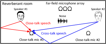
close-talk speech, cross-talk speech and environmental noises, all of which are reverberant. Inside close-talk mixtures, the close-talk speech usually has a strong energy, and inside close-talk speech, the direct-path signal of the target speaker is typically much stronger than reverberation. However, besides close-talk speech, close-talk mixtures often contain significant cross-talk speech produced by other speakers, especially if the other speakers, while talking, are spatially close to the target speaker. The contamination of cross-talk speech dramatically limits the application range of close-talk mixtures. For example, they are seldomly exploited as supervisions for training far-field speech separation models or leveraged as reference signals for evaluating speech separation models. It is a common perception that they are not suitable for these purposes as they are not clean enough Barker et al. (2018); Haeb-Umbach et al. (2019); Wisdom et al. (2020); Watanabe et al. (2020); Sivaraman et al. (2022); Aralikatti et al. (2023); Cornell et al. (2023); Leglaive et al. (2023).
This paper aims at reducing cross-talk speech and separating close-talk speech in close-talk mixtures. We name this task cross-talk reduction. Solving this task could enable many applications. For example, we can (a) leverage separated close-talk speech as pseudo-labels for training supervised far-field separation models; (b) use it as reference signals to evaluate the separation results of far-field separation models; and (c) present it rather than close-talk mixtures to annotators to reduce their annotation efforts.
One possible approach for cross-talk reduction is supervised speech separation Wang and Chen (2018); Yin et al. (2020); Jenrungrot et al. (2020); Tang et al. (2020); Nachmani et al. (2020); Rixen and Renz (2022); Wang et al. (2023c), where synthetic pairs of clean close-talk speech and close-talk (and far-field) mixtures are first synthesized via room simulation and then used to train supervised learning based models to predict the clean close-talk speech from its paired mixtures. The trained models, however, are known to suffer from severe generalization issues, as the simulated data used for training is often and inevitably mismatched with real-recorded test data Wang and Chen (2018); Pandey and Wang (2020); Tzinis et al. (2021); Zhang et al. (2021); Tzinis et al. (2022a, b); Leglaive et al. (2023).
Given only paired real-recorded far-field and close-talk mixtures, we propose to tackle cross-talk reduction by training unsupervised speech separation models directly on the real-recorded mixtures. This way, we can avoid the effort of data simulation, and the issues incurred when using simulated data. We point out that many existing unsupervised separation algorithms could be employed for cross-talk reduction. In this paper, we design a potentially better unsupervised algorithm by leveraging the fact that, for each speaker, the close-talk speech in close-talk mixtures has a strong energy, which can provide an informative cue about what the target speech is. Our idea is that we can (a) roughly separate the close-talk speech from each close-talk mixture (this could be achieved with a reasonable performance since the SNR of close-talk speech is usually high); and (b) reverberate the separated close-talk speech of each speaker via linear filtering to identify, and then cancel out, the speaker’s cross-talk speech captured by the close-talk microphones of the other speakers. Based on this idea, we propose CTRnet, where, during training, close-talk and far-field mixtures are stacked as input for a deep neural network (DNN) to first produce an estimate for each close-talk speech, and then the cross-talk speech in each close-talk mixture is identified (and cancelled out) by linearly filtering the DNN estimates via a linear prediction algorithm such that the filtering results of all the speakers can add up to the mixture. This paper makes three major contributions:
-
•
We propose a novel task, cross-talk reduction.
-
•
We propose a novel solution, unsupervised CTRnet.
-
•
We further propose weakly-supervised CTRnet, where, during training, speaker-activity timestamps are leveraged as a weak supervision to improve unsupervised CTRnet.
Evaluation results on a simulated CTR task and on a real-recorded conversational speech separation and recognition task show the effectiveness and potential of CTRnet. A sound demo is provided in the link below.222See https://zqwang7.github.io/demos/CTRnet_demo/index.html
2 Related Work
To the best of our knowledge, we are the first studying cross-talk reduction. There are tasks with similar names such as cross-talk cancellation Bleil (2023) which deals with sound field manipulation in spatial audio, and cross-talk suppression Tripathi et al. (2022) in circuits design. They are not related to our task and algorithms.
CTRnet builds upon the UNSSOR algorithm Wang and Watanabe (2023), leveraging UNSSOR’s capability at unsupervised speech separation. UNSSOR is designed to perform unsupervised separation based on far-field mixtures, assuming compact microphone arrays, while unsupervised CTRnet performs separation based on not only far-field but also close-talk mixtures, dealing with distributed-array cases for a different task: cross-talk reduction. We further propose weakly-supervised CTRnet, which leverages speaker-activity timestamps as weak supervision and shows strong performance on real-recorded data. In contrast, UNSSOR deals with unsupervised separation and is only validated on simulated data.
3 Problem Formulation
In a reverberant enclosure with speakers (each wearing a close-talk microphone) and a -microphone far-field array (see Fig. 1 for an illustration), each of the recorded closed-talk and far-field mixtures can be respectively formulated in the short-time Fourier transform (STFT) domain as follows:
| (1) | ||||
| (2) |
where indexes frames, indexes frequencies, indexes speakers (and close-talk microphones), and indexes far-field microphones. , and in (1) respectively denote the STFT coefficients of the close-talk mixture, reverberant image of speaker , and non-speech signals captured by the close-talk microphone of speaker at time and frequency . Notice that we use subscript to index the close-talk microphones. Similarly, , and in (2) respectively denote the STFT coefficients of the far-field mixture, reverberant image of speaker , and non-speech signals captured at far-field microphone . In the rest of this paper, we refer to the corresponding spectrograms when dropping , , or in notations. is assumed as a weak and stationary noise term.
Based on the close-talk and far-field mixtures, we aim at estimating , the close-talk speech of each speaker .333In , symbol in the subscript denotes the close-talk microphone of speaker , and in the parenthesis indicates that the notation represents the reverberant image of speaker . is very clean and can be roughly viewed as the dry source signal.444Some reverberation of the source signal still exists in , but it is much weaker than the direct-path signal. While speaker is speaking, inside is usually stronger than the cross-talk speech by any other speaker (). With these understandings, we formulate the above physical models as (3) and (4), and formulate cross-talk reduction as a blind deconvolution problem in (3).
In detail, let denote the close-talk speech of speaker , we re-formulate (1) as
| (3) |
where, in the second row, stacks a window of T-F units, is a sub-band filter, and computes Hermitian transpose. In (3), we leverage narrow-band approximation Talmon et al. (2009); Gannot et al. (2017); Wang (2024) to approximate (i.e., cross-talk speech of speaker captured by the close-talk microphone of speaker ) as a linear convolution between a filter and the close-talk speech of speaker , i.e., . This is reasonable since can be roughly viewed as the dry source signal, and, in this case, we can interpret the filter as the acoustic transfer function from speaker to close-talk microphone . In (3), contains the non-speech signal and absorbs the modeling errors incurred by using narrow-band approximation.
Similarly, for each far-field mixture, we re-formulate (2) as
| (4) |
where can be interpreted as the acoustic transfer function from speaker to far-field microphone .
Assuming that is weak, time-invariant and Gaussian, we can realize cross-talk reduction by solving, e.g., the problem below, which finds the sources, , and filters, , most consistent with the physical models in (3) and (4):
| (5) |
where computes magnitude. This is a blind deconvolution problem Levin et al. (2011) in artificial intelligence and machine learning, which is highly non-convex and not solvable if no prior knowledge is assumed about the sources or the filters, since all of them are unknown and need to be estimated.
Motivated by the classic expectation-maximization algorithm in machine learning Bishop (2006) and the recent UNSSOR algorithm Wang and Watanabe (2023), we propose to tackle this problem by leveraging unsupervised and weakly-supervised deep learning, where (a) a DNN is trained to first produce an estimate for each source (hence modeling source priors); (b) with the sources estimated, filter estimation in (3) then becomes a much simpler linear regression problem, where a closed-form solution exists and can be readily computed; and (c) loss functions similar to the objective in (3) can be designed to regularize the DNN estimates to have them respectively approximate the close-talk speech of each speaker.
4 Unsupervised CTRnet
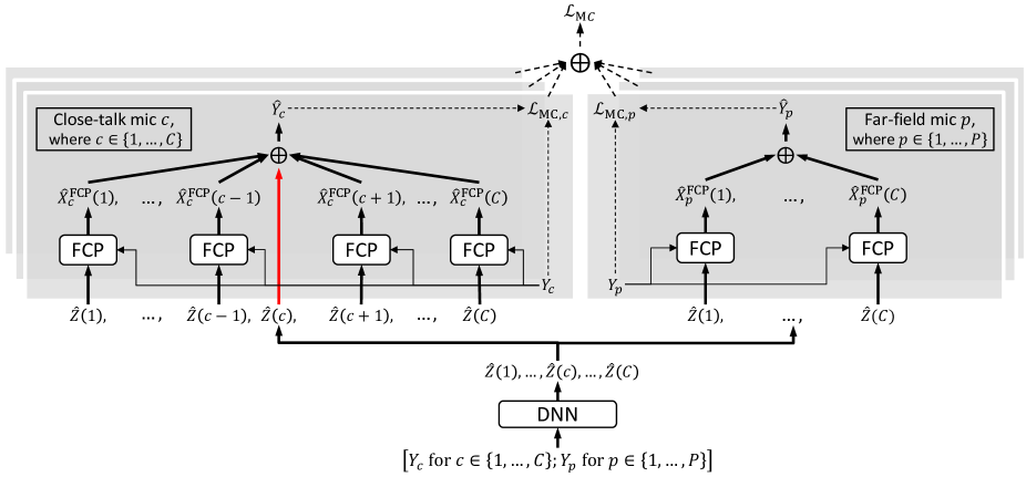
Fig. 2 illustrates unsupervised CTRnet. Given close-talk and far-field mixtures that are reasonably time-synchronized, it stacks close-talk and far-field mixtures as input, and produces, for each speaker , an estimate , which, we will show, is regularized to be an estimate for close-talk speech . Since can be viewed as the dry source signal, we can reverberate its estimate via a linear filtering algorithm named forward convolutive prediction (FCP) Wang et al. (2021b) to identify speaker ’s cross-talk speech at the close-talk microphones of the other speakers, as well as its reverberant images at far-field microphones. We realize this identification by training the DNN to optimize a combination of two loss functions, which encourage the DNN estimates and their linear filtering results to sum up to the mixture at each microphone (so that the linear filtering results can correctly identify the cross-talk speech which we aim at reducing). At run time, is used as the estimate of the close-talk speech for each speaker . This section describes the DNN configurations, loss functions, and FCP filtering.
4.1 DNN Configurations
We stack the real and imaginary (RI) components of close-talk and far-field mixtures as input features for the DNN to predict for each speaker . We can use complex spectral mapping Tan and Wang (2020); Wang et al. (2021a), where the DNN is trained to directly predict the RI components of for each speaker , or complex ratio masking Williamson et al. (2016), where the DNN is trained to predict the RI components of a complex-valued mask for each speaker and is then computed via , with denoting point-wise multiplication. The details of the DNN architecture are provided in Section 6.3, and the loss functions in the next subsection.
4.2 Mixture-Constraint Loss
We propose the following mixture-constraint (MC) loss:
| (6) |
where is the MC loss at close-talk microphone , at far-field microphone , and a weighting term.
Following the physical model in (3) and the first term in (3), at close-talk microphone we define as
| (7) |
where, in the third row, stacks a window of T-F units, and is a sub-band FCP filter to be described later in Section 4.3. From row to , we constrain the DNN estimate of each speaker to be a gain- and time-aligned estimate of the close-talk speech (i.e., ); and, for the reverberant image of each of the other speakers (i.e., cross-talk speech with ), we approximate it by linearly filtering (i.e., ). Since is constrained to approximate , which can be viewed as the dry source signal, it is very reasonable to linearly filter to estimate the image of speaker at the close-talk microphone of a different speaker and at far-field microphones. The estimated speaker images are then added together to reconstruct the mixture: , which is reasonable under the assumption that the non-speech signal is weak. Finally, we compute a loss between the reconstructed mixture and the mixture , by using a function , which computes an absolute loss on the estimated RI components and their magnitude Wang et al. (2023c):
where is a set of functions with extracting the real part, the imaginary part and the magnitude of a complex number, and the denominator balances the losses across different microphones and training mixtures.
Similarly, at far-field microphone we define as
| (8) |
where we linearly filter the DNN estimate for each speaker using so that their summation can approximate the mixture captured by far-field microphone .
4.3 FCP for Filter Estimation
To compute , we need to first estimate the linear filters, each of which is the relative transfer function relating the close-talk speech of a speaker to the speaker’s reverberant image captured by a distant microphone. Following UNSSOR Wang and Watanabe (2023), we employ FCP Wang et al. (2021b) to estimate them.
Assuming speakers are non-moving within each utterance, we estimate the filters by solving the following problem:
| (9) |
where symbol is used to index the far-field and close-talk microphones, and and are defined below (4.2). is a weighting term balancing the importance of each T-F unit, and following Wang et al. (2021b), for each close-talk microphone and speaker , it is defined as
| (10) |
where floors the weighting term and extracts the maximum value of a power spectrogram; and for each far-field microphone and speaker , it is defined as
| (11) |
We compute the weighting term individually for each microphone, considering that each speaker has different energy levels at different microphones. (4.3) is a weighted linear regression problem, where a closed-form solution can be computed:
where computes complex conjugate. We then plug it into (4.2) and (4.2), compute the losses, and train the DNN.
Although, in (4.3), is filtered to approximate , earlier studies Wang et al. (2021b) have suggested that the filtering result would approximate (see the derivation in Appendix C of Wang and Watanabe (2023)), if is sufficiently accurate, which can be reasonably satisfied as the close-talk speech in close-talk mixtures already has a high input SNR. The estimated speaker image is named FCP-estimated image Wang and Watanabe (2023):
| (12) |
We can hence sum up the FCP-estimated images and compare the summation with in (4.2) and (4.2). Notice that the FCP-estimated images at close-talk microphones represent the identified cross-talk speech we aim to reduce.
5 Weakly-Supervised CTRnet
We propose to leverage speaker-activity timestamps as a weak supervision to improve the training of unsupervised CTRnet. For each speaker , its activity timestamps are denoted as a binary vector , where is signal length in samples, and value means that speaker is active at a sample and otherwise. Note that speaker-activity timestamps are provided in almost every conversational speech recognition dataset. They are annotated by having human annotators listen to close-talk mixtures. This section describes why and how the timestamps can help training CTRnet.
5.1 Motivation
In human conversations where concurrent speech naturally happens, speaker overlap is often sparse. See Appendix B for an example. This sparsity poses major difficulties for speech separation Chen et al. (2020); Cosentino et al. (2020), as the number of concurrent speakers is time-varying. Modern separation models usually assume a maximum number of speakers the models can separate, but the models could over- or under-separate the speakers due to errors in speaker counting.
Assuming that there are at maximum speakers in each processing segment, unsupervised CTRnet, in essence, learns to produce output spectrograms that can be filtered to best explain the recorded close-talk and far-field mixtures. One issue is that, in some training segments, if there are fewer than speakers, unsupervised CTRnet would always over-separate the speakers to obtain a smaller loss.555This is similar to unsupervised clustering. Hypothesizing more clusters for clustering can almost always produce a smaller objective but some clusters are split into smaller ones Bishop (2006). Therefore, the knowledge about the accurate number of speakers, which can be provided by speaker-activity timestamps, can be very useful to improve the training of unsupervised CTRnet.
Meanwhile, we find that unsupervised CTRnet usually cannot produce zero predictions in the silent ranges of each speaker. In these ranges, the predicted spectrogram for each speaker often contains weak but non-negligible and intelligible signals from the other speakers. This is a common problem in conversational speech separation Wang et al. (2021a); Morrone et al. (2023). In unsupervised CTRnet, this often results in a smaller loss, as the FCP filtering procedure could better approximate close-talk and far-field mixtures by filtering the non-zero predictions in silent regions.
With these understandings, we leverage speaker-activity timestamps in the following two ways to better train CTRnet.
5.2 Muting during Training
During training, we propose to mute all or part of the frames in each based on the speaker-activity timestamps , before computing the filters and loss. In detail, we compute
| (13) |
where , defined based on , is if the STFT window corresponding to frame contains any active speech samples of speaker and is otherwise, and is if contains at least second of active speech in the training segment and is otherwise. Using for muting frames and for muting speakers, we can avoid using non-zero predictions in silent ranges for FCP. We then replace with in (4.2), (4.2) and (4.3) to compute FCP filters and for DNN training. This way, CTRnet could more robustly reduce cross-talk speech for up to speakers.
5.3 Speaker-Activity Loss
We propose a speaker-activity (SA) loss that can encourage the DNN-estimated signal for each speaker to be zero in silent ranges marked by speaker-activity timestamps:
| (14) |
where and are defined in the first paragraph of Section 5, computes the norm, is the re-synthesized time-domain signal of obtained by applying inverse STFT (iSTFT) to , is the time-domain close-talk mixture signal of speaker , and the second term is a scaling factor accounting for the fact that each speaker usually has different length of silence in each training segment. We combine it with in (6) for training:
| (15) |
where is a weighting term. penalizes prediction errors in non-silent ranges of each speaker when muting is used, while penalizes predictions in silent ranges.
6 Experimental Setup
There are no existing studies on cross-talk reduction. We first evaluate unsupervised CTRnet on a simulated dataset named SMS-WSJ-FF-CT, where clean signals can be available for metric computation, and then evaluate weakly-supervised CTRnet on a real-recorded conversational automatic speech recognition (ASR) dataset named CHiME-7, using ASR metrics for evaluation. This section describes the datasets, system setups, comparison systems, and evaluation metrics.
6.1 SMS-WSJ-FF-CT and Evaluation Setup
SMS-WSJ-FF-CT, with “FF” meaning far-field and “CT” close-talk, is built upon a simulated dataset named SMS-WSJ Drude et al. (2019) which consists of -speaker fully-overlapped noisy-reverberant mixtures, by simulating a close-talk microphone for each speaker. Fig. 1 shows this setup. This evaluation serves as a proof of concept to validate whether CTRnet can work well in ideal cases, where the hypothesized physical models in (3) and (4) are largely satisfied.
SMS-WSJ Drude et al. (2019), a popular corpus for evaluating -speaker separation algorithms in reverberant conditions, has ( h), ( h) and ( h) -speaker mixtures for training, validation and testing. The clean speech is sampled from the WSJ0 and WSJ1 corpus. The simulated far-field microphone array has microphones uniformly placed on a circle with a diameter of cm. For each mixture, the speaker-to-array distance is sampled from the range m, and the reverberation time (T60) from s. A weak white noise is added to simulate microphone self-noises, at an energy level between the summation of the reverberant speech signals and the noise sampled from the range dB. The sampling rate is 8 kHz.
SMS-WSJ-FF-CT is simulated by adding a close-talk microphone for each of the speakers in each SMS-WSJ mixture. In each mixture, the distance from each speaker to its close-talk microphone is uniformly sampled from the range m, and the angle from . All the other setup remains unchanged. This way, we can obtain the close-talk mixture of each speaker, and the far-field mixtures are exactly the same as those in SMS-WSJ.
Training and Inference of CTRnet. For training, in default we sample an -second segment from each mixture in each epoch, and the batch size is . For inference, we feed each test mixture in its full length to CTRnet.
Evaluation Metrics. For each speaker , we use its time-domain close-talk speech corresponding to as the reference signal for evaluation. The evaluation metrics include signal-to-distortion ratio (SDR) Vincent et al. (2006), scale-invariant SDR (SI-SDR) Le Roux et al. (2019), perceptual evaluation of speech quality (PESQ) Rix et al. (2001), and extended short-time objective intelligibility (eSTOI) Taal et al. (2011). All of them are widely-used in speech separation.
Comparison Systems include signal processing based unsupervised speech separation algorithms, cACGMM-based spatial clustering (SC) Boeddeker et al. (2021) and independent vector analysis (IVA) Sawada et al. (2019). Both are very popular. We stack close-talk and far-field mixtures as input. For SC, we use a public implementation Boeddeker (2019) provided in the pb_bss toolkit; and for IVA, we use the torchiva toolkit Scheibler and Saijo (2022). The STFT window and hop sizes are tuned to 128 and 16 ms for SC, and to 256 and 32 ms for IVA. For IVA, we use the Gaussian model in torchiva to model source distribution. A garbage source is used in both models to absorb modeling errors.
6.2 CHiME-7 and Evaluation Setup
To show that CTRnet can work on realistic data, we train and evaluate CTRnet using the real-recorded CHiME-7 dataset, following the setup of the CHiME-7 DASR challenge Cornell et al. (2023). CHiME-7, built upon CHiME-{5,6} Watanabe et al. (2020); Barker et al. (2018), is a notoriously difficult dataset in conversational speech separation and recognition, mainly due to its realisticness, which is representative of common problems deployed systems could run into in practice, such as microphone synchronization errors, signal clipping, frame dropping, microphone failures, moving arrays, moving speakers, varying degrees of speaker overlap, and challenging environmental noises. So far, the most successful separation algorithm for CHiME-7 is still based on guided source separation (GSS) Boeddecker et al. (2018), a signal processing algorithm, and supervised DNN-based approaches have nearly no success on this dataset. All the top teams in CHiME-7 Wang et al. (2023a); Ye et al. (2023) and in similar challenges or datasets, e.g., AliMeeting Yu et al. (2022); Liang et al. (2023) and AMI Raj et al. (2023), all adopt GSS as the only separation module. This section describes the dataset and our evaluation setup.
CHiME-7 Dataset contains real-recorded conversational sessions, each with participants speaking spontaneously in a domestic, dinner-party scenario, where concurrent speech can naturally happen. Each speaker (participant) wears a binaural close-talk microphone, and there are Kinect devices, each with microphones, placed in a strategic way in the room to record each entire session, which is to hours long. The recorded close-talk mixtures contain severe cross-talk speech. Realistic noises typical in dinner parties are recorded at the same time along with speech. There are 14 ( h), 2 ( h) and 4 ( h) recorded sessions respectively for training, validation and testing. The sampling rate is kHz.
Experiment Design. Based on the CHiME-7 dataset, we design an experiment for cross-talk reduction. We consider the mixture recorded at the right ear of each binaural microphone as the close-talk mixture and the one at the left ear as far-field mixture, meaning that we have close-talk and far-field mixtures.
Training and Inference of CTRnet. To train CTRnet, we cut each (long) session into -second segments with overlap between consecutive segments, and train CTRnet on these segments. At inference time, we apply the trained CTRnet in a block-wise way to process each (long) session. The final separated speech for each speaker has the same length as the (long) input session. See Appendix A for the details.
Evaluation Metrics. With the separated signal of each speaker, following the CHiME-7 DASR challenge Cornell et al. (2023) we compute diarization-assigned word error rates (DA-WER). In detail, the separated signal of each speaker is split to short utterances by using oracle speaker-activity timestamps, and the default, pre-trained ASR model provided by the challenge is used to recognize and score each utterance. The pre-trained ASR model666https://huggingface.co/popcornell/chime7_task1_asr1_baseline is a strong end-to-end model based on a transformer encoder/decoder architecture trained with joint CTC/attention, using WavLM features.
| Row | Systems | Masking/Mapping | SI-SDR (dB) | SDR (dB) | PESQ | eSTOI | ||||||
| 0 | Unprocessed mixture | - | - | - | - | - | - | - | ||||
| 1a | Unsupervised CTRnet | Mapping | ||||||||||
| 1b | Unsupervised CTRnet | Mapping | ||||||||||
| 1c | Unsupervised CTRnet | Mapping | ||||||||||
| 1d | Unsupervised CTRnet | Mapping | ||||||||||
| 2 | Unsupervised CTRnet | Masking | ||||||||||
| 3a | Unsupervised CTRnet | Mapping | ||||||||||
| 3b | Unsupervised CTRnet | Mapping | ||||||||||
| 3c | Unsupervised CTRnet | Mapping | ||||||||||
| 3d | Unsupervised CTRnet | Mapping | ||||||||||
| 4a | Unsupervised CTRnet | Mapping | ||||||||||
| 4b | Unsupervised CTRnet | Mapping | ||||||||||
| 4c | Unsupervised CTRnet | Mapping | ||||||||||
| 5a | Unsupervised CTRnet | Mapping | ||||||||||
| 5b | Unsupervised CTRnet | Mapping | ||||||||||
| 5c | Unsupervised CTRnet | Mapping | ||||||||||
| 6 | Unsupervised CTRnet | Mapping | ||||||||||
| 7a | SC Boeddeker (2019) | - | - | - | - | - | - | |||||
| 7b | IVA Scheibler and Saijo (2022) | - | - | - | - | - | - |
Comparison Systems. We use GSS Boeddecker et al. (2018) for comparison, by following the implementation provided in CHiME-7 DASR Challenge.777See https://github.com/espnet/espnet/blob/master/egs2/chime7_ task1/asr1/local/run_gss.sh GSS is the most popular and effective separation model so far for modern ASR systems. It first performs dereverberation using the weighted prediction algorithm Nakatani et al. (2010) and then computes a mask-based beamformer for separation by using posterior time-frequency masks estimated by a spatial clustering module guided by oracle speaker-activity timestamps Boeddecker et al. (2018). Notice that at run time GSS requires oracle speaker-activity timestamps, while weakly-supervised CTRnet only needs them for training and, once trained, no longer needs them. Another note is that the training data of the pre-trained ASR model provided by the challenge contains GSS-processed signals, and is hence favorable to GSS.
6.3 Miscellaneous Configurations of CTRnet
For STFT, the window size is ms, hop size ms, and the square root of the Hann window is used as the analysis window. TF-GridNet Wang et al. (2023c) is employed as the DNN architecture. Using the symbols defined in Table I of Wang et al. (2023c), we set its hyper-parameters to , , , , , and (please do not confuse these symbols with the ones defined in this paper). The model has around million parameters. in (10) and (11) is tuned to . in (15) is set to .
7 Evaluation Results and Discussions
7.1 Results on SMS-WSJ-FF-CT
Table 1 configures unsupervised CTRnet in various ways and presents the results on SMS-WSJ-FF-CT. Row reports the scores of unprocessed mixtures. The dB SI-SDR indicates that the close-talk mixtures are not clean due to the contamination by cross-talk speech. In 1a-1d, we vary the number of FCP filter taps and configure the FCP filters to be causal by setting . We observe that the setup in 1b obtains the best SI-SDR. In row , complex masking rather than mapping is used to obtain , but the result is not better than 1b. In 3a-3d, we reduce in (6) from to and so that the loss on close-talk mixtures is emphasized. This is reasonable since we aim at separating close-talk speech, rather than far-field speaker images. From 1b and 3b, we observe that this change leads to clear improvement (e.g., from to dB SI-SDR). In 4a-4c, we use non-causal FCP filters by increasing from to , and , while fixing the total number of filter taps to . This does not yield improvements, likely because is regularized to be an estimate of the close-talk speech of speaker and hence the transfer function relating it to speaker ’s reverberant images at other microphones should be largely causal. In 5a-5c, we reduce the number of far-field microphones from to , and . That is, we only use microphone (a) ; (b) and ; and (c) , and of the far-field six-microphone array to simulate the cases when the far-field array only has a limited number of microphones. Compared with 3b, the performance drops, indicating the benefits of using more far-field mixtures as network input and for loss computation, while the improvement over the mixture scores in row is still large. In default, our models are trained using mini-batches of 4 four-second segments, while, in row , we train the model by using a batch size of and using each training mixture in its full length. This improves SI-SDR over 3b, likely because better FCP filters can be computed during training by using all the frames in each mixture.
In row 7a and 7b, SC and IVA perform worse than CTRnet. SC does not work well, possibly because, in this distributed-microphone scenario where each speaker signal can have very different SNRs at different microphones, the target T-F masks at different microphones are significantly different.
| DA-WER (%) | ||||||||
| Row | Systems | Muting? | Val. | Test | ||||
| 0 | Unprocessed mixture | - | - | - | 4 | - | ||
| 1 | Unsupervised CTRnet | - | ||||||
| 2 | Weakly-supervised CTRnet | ✗ | ||||||
| 3 | Weakly-supervised CTRnet | ✓ | ||||||
| 4 | GSS Boeddecker et al. (2018) | - | - | - | ||||
7.2 Results on CHiME-7
Table 2 reports the ASR results of CTRnet on the close-talk mixtures of CHiME-7. The filter taps and are tuned to and . Notice that, here, one future tap is used, as the real-recorded data in CHiME-7 exhibits non-negligible synchronization errors among different microphone signals and we find that allowing one future tap can mitigate the synchronization issues. Complex spectral mapping is used in default.
In row , the mixture DA-WER is high even though a strong pre-trained ASR model is used for recognition. This is because the close-talk mixtures contain very strong cross-talk speech, which confuses the ASR model on which speaker to recognize. In row , using unsupervised CTRnet to reduce cross-talk speech produces clear improvement (from to DA-WER). In row , weakly-supervised CTRnet with muting during training further improves the performance to . In row , muting is not applied when training weakly-supervised CTRnet, and we observe much worse DA-WER. We found that this is because, without using muting, the loss in (15) tends to push of each speaker towards zeros to obtain a smaller loss value. Compared with GSS, weakly-supervised CTRnet, through learning, obtains clearly better DA-WER (i.e., vs. ). In addition, clear improvement is obtained over the unprocessed mixtures (i.e., vs. ). These results indicate the effectiveness of CTRnet for cross-talk reduction on real-recorded data.
8 Conclusion
We have proposed a novel task, cross-talk reduction, and a novel solution, CTRnet, with or without leveraging speaker-activity timestamps for model training. A key contribution of this paper, we emphasize, is that the proposed CTRnet can be trained directly on real-recorded pairs of far-field and close-talk mixtures, and is capable of effectively reducing cross-talk speech, especially on the notoriously difficult real-recorded CHiME-7 data. This contribution suggests a promising way towards addressing a fundamental limitation of real-recorded close-talk speech. That is, the contamination by cross-talk speech, which makes close-talk mixtures not sufficiently clean. With CTRnet producing reasonably-good cross-talk reduction, we expect many applications to be enabled, and we will investigate them in our future work.
In closing, another key contribution of this paper, we point out, is that the proposed weakly-supervised deep learning based methodology for blind deconvolution can work well on challenging real-recorded data. This contribution, we believe, would motivate a new stream of research towards realizing robust neural speech separation in realistic conditions, and generate broader impact beyond CTR and speech separation, especially in many machine learning and artificial intelligence applications where the sensors would not only capture target signals but also interference signals very detrimental to machine perception.
Appendix A Run-Time Separation of Long Sessions
In CHiME-, the duration of each recorded session ranges from to hours. At run time, to separate the close-talk speech of an entire session, we run CTRNet in a block-wise way, using the pseudo-code below at each processing block:
| (16) | ||||
| (17) | ||||
| (18) | ||||
| (19) |
where and are respectively the sample-level standard deviations of the time-domain close-talk mixture and far-field mixture . After obtaining at each block, we stack of all the processing blocks and then revert the stacked spectrogram to time domain via inverse STFT. Notice that in (4.2) constrains each close-talk speech estimate to have the same gain level as the close-talk mixture , by not filtering . As a result, in (18), each output is expected to have the same gain level as .
For our experiments on CHiME-, the processing block size is set to seconds, the same as the segment length used during training. We configure the blocks to be slightly overlapped, where we consider the first and the last seconds as context, and output the DNN estimates in the center () seconds at each block.
Appendix B Illustration of Sparse Speaker Overlap
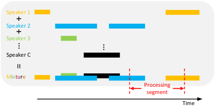
Fig. 3 illustrates sparse speaker overlap in human conversations. This sparsity is because, for conversations in, e.g., meeting or dinner-party scenarios, people often take turns to speak and tend to not always speak at the same time. As a result, in different (short) processing segments of separation systems, the number of active speakers and the degrees of speaker overlap can vary a lot.
Acknowledgments
Experiments of this work used the Bridges2 system at PSC and Delta at NCSA through allocation CIS and IRIP from the Advanced Cyberinfrastructure Coordination Ecosystem: Services and Support (ACCESS) program, which is supported by National Science Foundation grants #, #, #, # and #.
References
- Aralikatti et al. [2023] Rohith Aralikatti, Christoph Boeddeker, Gordon Wichern, et al. Reverberation as Supervision for Speech Separation. In ICASSP, 2023.
- Barker et al. [2018] Jon Barker, Shinji Watanabe, Emmanuel Vincent, et al. The Fifth ’CHiME’ Speech Separation and Recognition Challenge: Dataset, Task and Baselines. In Interspeech, pages 1561–1565, 2018.
- Bishop [2006] C. M. Bishop. Pattern Recognition and Machine Learning. Springer, 2006.
- Bleil [2023] Jacob Bleil. Systematic Development of a Phased Speaker Array for Optimal 3D Audio Reproduction. PhD thesis, Princeton University, 2023.
- Boeddecker et al. [2018] Christoph Boeddecker, Jens Heitkaemper, Joerg Schmalenstroeer, Lukas Drude, Jahn Heymann, et al. Front-End Processing for The CHiME-5 Dinner Party Scenario. In CHiME, pages 35–40, 2018.
- Boeddeker et al. [2021] Christoph Boeddeker, Frederik Rautenberg, et al. A Comparison and Combination of Unsupervised Blind Source Separation Techniques. In Speech Communication, pages 129–133, 2021.
- Boeddeker [2019] Christoph Boeddeker. pb_bss. https://github.com/fgnt/pb_bss/blob/master/examples/mixture_model_example.ipynb, 2019. Accessed: 2023-01-18.
- Carletta et al. [2006] Jean Carletta, Simone Ashby, Sebastien Bourban, Mike Flynn, Mael Guillemot, et al. The AMI Meeting Corpus: A Pre-Announcement. In Machine Learning for Multimodal Interaction, pages 28–39, 2006.
- Chen et al. [2020] Zhuo Chen, Takuya Yoshioka, Liang Lu, Tianyan Zhou, Zhong Meng, Yi Luo, Jian Wu, Xiong Xiao, and Jinyu Li. Continuous Speech Separation: Dataset and Analysis. In ICASSP, pages 7284–7288, 2020.
- Cornell et al. [2023] Samuele Cornell, Matthew S. Wiesner, Shinji Watanabe, et al. The CHiME-7 DASR Challenge: Distant Meeting Transcription with Multiple Devices in Diverse Scenarios. In CHiME, pages 1–6, 2023.
- Cosentino et al. [2020] Joris Cosentino, Manuel Pariente, Samuele Cornell, Antoine Deleforge, et al. LibriMix: An Open-Source Dataset for Generalizable Speech Separation. In arXiv preprint arXiv:2005.11262, 2020.
- Drude et al. [2019] Lukas Drude, Jens Heitkaemper, Christoph Boeddeker, and Reinhold Haeb-Umbach. SMS-WSJ: Database, Performance Measures, and Baseline Recipe for Multi-Channel Source Separation and Recognition. In arXiv preprint arXiv:1910.13934, 2019.
- Gannot et al. [2017] Sharon Gannot, Emmanuel Vincent, Shmulik Markovich-Golan, and Alexey Ozerov. A Consolidated Perspective on Multi-Microphone Speech Enhancement and Source Separation. IEEE/ACM Trans. Audio, Speech, Lang. Proc., 25:692–730, 2017.
- Haeb-Umbach et al. [2019] Reinhold Haeb-Umbach, Shinji Watanabe, Tomohiro Nakatani, Michiel Bacchiani, et al. Speech Processing for Digital Home Assistants: Combining Signal Processing with Deep-Learning Techniques. IEEE Signal Processing Magazine, 36(6):111–124, 2019.
- Jenrungrot et al. [2020] Teerapat Jenrungrot, Vivek Jayaram, Steve Seitz, and Ira Kemelmacher-Shlizerman. The Cone of Silence: Speech Separation by Localization. In NeurIPS, 2020.
- Le Roux et al. [2019] Jonathan Le Roux, Scott Wisdom, Hakan Erdogan, and John R Hershey. SDR - Half-Baked or Well Done? In ICASSP, pages 626–630, 2019.
- Leglaive et al. [2023] Simon Leglaive, Léonie Borne, Efthymios Tzinis, Mostafa Sadeghi, et al. The CHiME-7 UDASE Task: Unsupervised Domain Adaptation for Conversational Speech Enhancement. In CHiME, 2023.
- Levin et al. [2011] Anat Levin, Yair Weiss, Fredo Durand, and William T. Freeman. Understanding Blind Deconvolution Algorithms. IEEE Trans. Pattern Anal. Mach. Intell., 33(12):2354–2367, 2011.
- Liang et al. [2023] Yuhao Liang, Mohan Shi, Fan Yu, Yangze Li, et al. The Second Multi-Channel Multi-Party Meeting Transcription Challenge (M2MeT 2.0): A Benchmark for Speaker-Attributed ASR. In ASRU, 2023.
- Morrone et al. [2023] Giovanni Morrone, Samuele Cornell, Desh Raj, Luca Serafini, Enrico Zovato, et al. Low-Latency Speech Separation Guided Diarization for Telephone Conversations. In SLT, pages 641–646, 2023.
- Nachmani et al. [2020] Eliya Nachmani, Yossi Adi, and Lior Wolf. Voice Separation with An Unknown Number of Multiple Speakers. In ICML, pages 7121–7132, 2020.
- Nakatani et al. [2010] Tomohiro Nakatani, Takuya Yoshioka, et al. Speech Dereverberation Based on Variance-Normalized Delayed Linear Prediction. IEEE Trans. Audio, Speech, Lang. Proc., 18(7):1717–1731, 2010.
- Pandey and Wang [2020] Ashutosh Pandey and DeLiang Wang. On Cross-Corpus Generalization of Deep Learning Based Speech Enhancement. IEEE/ACM Trans. Audio, Speech, Lang. Proc., 28:2489–2499, 2020.
- Raj et al. [2023] Desh Raj, Daniel Povey, et al. GPU-Accelerated Guided Source Separation for Meeting Transcription. In Interspeech, pages 3507–3511, 2023.
- Rix et al. [2001] Antony W. Rix, John G. Beerends, et al. Perceptual Evaluation of Speech Quality (PESQ)-A New Method for Speech Quality Assessment of Telephone Networks and Codecs. In ICASSP, pages 749–752, 2001.
- Rixen and Renz [2022] Joel Rixen and Matthias Renz. SFSRNet: Super-Resolution for Single-Channel Audio Source Separation. In AAAI, 2022.
- Sawada et al. [2019] Hiroshi Sawada, Nobutaka Ono, Hirokazu Kameoka, Daichi Kitamura, et al. A Review of Blind Source Separation Methods: Two Converging Routes to ILRMA Originating from ICA and NMF. APSIPA Trans. Signal and Info. Proc., 8:1–14, 2019.
- Scheibler and Saijo [2022] Robin Scheibler and Kohei Saijo. Torchiva. https://github.com/fakufaku/torchiva, 2022. Accessed: 2023-01-18.
- Sivaraman et al. [2022] Aswin Sivaraman, Scott Wisdom, Hakan Erdogan, and John R. Hershey. Adapting Speech Separation To Real-World Meetings Using Mixture Invariant Training. In ICASSP, pages 686–690, 2022.
- Taal et al. [2011] Cees H. Taal, Richard C. Hendriks, et al. An Algorithm for Intelligibility Prediction of Time-Frequency Weighted Noisy Speech. IEEE Trans. Audio, Speech, Lang. Proc., 19(7):2125–2136, 2011.
- Talmon et al. [2009] Ronen Talmon, Israel Cohen, et al. Relative Transfer Function Identification using Convolutive Transfer Function Approximation. IEEE Trans. Audio, Speech, Lang. Proc., 17(4):546–555, 2009.
- Tan and Wang [2020] Ke Tan and DeLiang Wang. Learning Complex Spectral Mapping With Gated Convolutional Recurrent Networks for Monaural Speech Enhancement. IEEE/ACM Trans. Audio, Speech, Lang. Proc., 28:380–390, 2020.
- Tang et al. [2020] Chuanxin Tang, Chong Luo, Zhiyuan Zhao, Wenxuan Xie, and Wenjun Zeng. Joint Time-Frequency and Time Domain Learning for Speech Enhancement. In IJCAI, pages 3816–3822, 2020.
- Tripathi et al. [2022] Vinay Tripathi, Huo Chen, Mostafa Khezri, Ka Wa Yip, et al. Suppression of Crosstalk in Superconducting Qubits using Dynamical Decoupling. Physical Review Applied, 18(2), 2022.
- Tzinis et al. [2021] Efthymios Tzinis, Scott Wisdom, Aren Jansen, Shawn Hershey, Tal Remez, et al. Into the Wild with AudioScope: Unsupervised Audio-Visual Separation of On-Screen Sounds. In ICLR, 2021.
- Tzinis et al. [2022a] Efthymios Tzinis, Yossi Adi, Vamsi K. Ithapu, Buye Xu, Paris Smaragdis, and Anurag Kumar. RemixIT: Continual Self-Training of Speech Enhancement Models via Bootstrapped Remixing. IEEE J. of Selected Topics in Signal Proc., 16(6):1329–1341, 2022.
- Tzinis et al. [2022b] Efthymios Tzinis, Scott Wisdom, Tal Remez, and John R. Hershey. AudioScopeV2: Audio-Visual Attention Architectures for Calibrated Open-Domain On-Screen Sound Separation. In ECCV, pages 368–385, 2022.
- Vincent et al. [2006] Emmanuel Vincent, Rémi Gribonval, and Cédric Févotte. Performance Measurement in Blind Audio Source Separation. IEEE Trans. Audio, Speech, Lang. Proc., 14(4):1462–1469, 2006.
- Wang and Chen [2018] DeLiang Wang and Jitong Chen. Supervised Speech Separation Based on Deep Learning: An Overview. IEEE/ACM Trans. Audio, Speech, Lang. Proc., 26(10):1702–1726, 2018.
- Wang and Watanabe [2023] Zhong-Qiu Wang and Shinji Watanabe. UNSSOR: Unsupervised Neural Speech Separation by Leveraging Over-determined Training Mixtures. In NeurIPS, 2023.
- Wang et al. [2021a] Zhong-Qiu Wang, Peidong Wang, and DeLiang Wang. Multi-Microphone Complex Spectral Mapping for Utterance-Wise and Continuous Speech Separation. IEEE/ACM Trans. Audio, Speech, Lang. Proc., 29:2001–2014, 2021.
- Wang et al. [2021b] Zhong-Qiu Wang, Gordon Wichern, and Jonathan Le Roux. Convolutive Prediction for Monaural Speech Dereverberation and Noisy-Reverberant Speaker Separation. IEEE/ACM Trans. Audio, Speech, Lang. Proc., 29:3476–3490, 2021.
- Wang et al. [2023a] Ruoyu Wang, Maokui He, Jun Du, et al. The USTC-NERCSLIP Systems for the CHiME-7 DASR Challenge. In CHiME, pages 13–18, 2023.
- Wang et al. [2023b] Zhe Wang, Shilong Wu, Hang Chen, et al. The Multimodal Information Based Speech Processing (MISP) 2022 Challenge: Audio-Visual Diarization And Recognition. In ICASSP, pages 1–5, 2023.
- Wang et al. [2023c] Zhong-Qiu Wang, Samuele Cornell, Shukjae Choi, et al. TF-GridNet: Integrating Full- and Sub-Band Modeling for Speech Separation. IEEE/ACM Trans. Audio, Speech, Lang. Proc., 31:3221–3236, 2023.
- Wang [2024] Zhong-Qiu Wang. USDnet: Unsupervised Speech Dereverberation via Neural Forward Filtering. arXiv preprint arXiv:2402.00820, 2024.
- Watanabe et al. [2020] Shinji Watanabe, Michael Mandel, Jon Barker, et al. CHiME-6 Challenge: Tackling Multispeaker Speech Recognition for Unsegmented Recordings. In arXiv preprint arXiv:2004.09249, 2020.
- Williamson et al. [2016] Donald S. Williamson, Yuxuan Wang, and DeLiang Wang. Complex Ratio Masking for Monaural Speech Separation. IEEE/ACM Trans. Audio, Speech, Lang. Proc., pages 483–492, 2016.
- Wisdom et al. [2020] Scott Wisdom, Efthymios Tzinis, Hakan Erdogan, Ron J. Weiss, Kevin Wilson, and John R. Hershey. Unsupervised Sound Separation using Mixture Invariant Training. In NeurIPS, 2020.
- Ye et al. [2023] Lingxuan Ye, Haitian Lu, Gaofeng Cheng, Yifan Chen, et al. The IACAS-Thinkit System for CHiME-7 Challenge. In CHiME, pages 23–26, 2023.
- Yin et al. [2020] Dacheng Yin, Chong Luo, Zhiwei Xiong, et al. PHASEN: A Phase-and-Harmonics-Aware Speech Enhancement Network. In AAAI, pages 9458–9465, 2020.
- Yu et al. [2022] Fan Yu, Shiliang Zhang, Pengcheng Guo, Yihui Fu, Zhihao Du, et al. Summary on The ICASSP 2022 Multi-Channel Multi-Party Meeting Transcription Grand Challenge. In ICASSP, pages 9156–9160, 2022.
- Zhang et al. [2021] Wangyou Zhang, Jing Shi, Chenda Li, Shinji Watanabe, et al. Closing The Gap Between Time-Domain Multi-Channel Speech Enhancement on Real and Simulation Conditions. In WASPAA, pages 146–150, 2021.