Quantitative Convergences of Lie Group Momentum Optimizers
Abstract
Explicit, momentum-based dynamics that optimize functions defined on Lie groups can be constructed via variational optimization and momentum trivialization. Structure preserving time discretizations can then turn this dynamics into optimization algorithms. This article investigates two types of discretization, Lie Heavy-Ball, which is a known splitting scheme, and Lie NAG-SC, which is newly proposed. Their convergence rates are explicitly quantified under -smoothness and local strong convexity assumptions. Lie NAG-SC provides acceleration over the momentumless case, i.e. Riemannian gradient descent, but Lie Heavy-Ball does not. When compared to existing accelerated optimizers for general manifolds, both Lie Heavy-Ball and Lie NAG-SC are computationally cheaper and easier to implement, thanks to their utilization of group structure. Only gradient oracle and exponential map are required, but not logarithm map or parallel transport which are computational costly.
1 Introduction
First order optimization, i.e., with gradient of the potential (i.e. the objective function) given as the oracle, is ubiquitously employed in machine learning. Within this class of algorithms, momentum is often introduced to accelerate convergence; for example, in Euclidean setups, it has been proved to yield the optimal dimension-independent convergence order, for a large class of first order optimizers, under strongly convex and -smooth assumptions of the objective function[16, Sec. 2].
Gradient Descent (GD) without momentum can be generalized to Riemannian manifold by moving to the negative gradient direction using the exponential map with a small step size. This generalization is algorithmically straight forward, but quantifying the convergence rate in curved spaces needs nontrivial efforts [5, 26, 22]. In comparison, generalizing momentum GD to manifold itself is nontrivial due to curved geometry; for example, the iteration must be kept on the manifold and the momentum must stay in the tangent space, which changes with the iteration, at the same time. It is even more challenging to quantify the convergence rate theoretically due to the loss of linearity in the space, leading to the lack of triangle inequality and cosine rule. Finally, there is not necessarily acceleration unless the generalization is done delicately.
Regardless, optimization on manifolds is an important task, for which the manifold structure can either naturally come from the problem setup or be artificially introduced. A simple but extremely important example is to compute the leading eigenvalues of a large matrix, which can be approached efficiently via optimization on the Stiefel manifold [14]; a smaller scale version can also be solved via optimization on [6, 23, 7, 21]. More on the modern machine learning side, one can algorithmically add orthonormal constraints to deep learning models to improve their accuracy and robustness [e.g., 4, 8, 12, 14, 19]. Both examples involve , which is an instance of an important type of curved spaces called Lie groups.
Lie groups are manifolds with additional group structure, and the nonlinearity of the space manifests through the non-commutative group multiplication. The group structure can help not only design momentum optimizer but also analyze its convergence. More precisely, this work will make the following contributions:
-
•
Provide the first quantitative analysis of Lie group momentum optimizers. This is significant, partly because there is no nontrivial convex functions on many Lie groups (see Rmk. 1), so we have to analyze nonconvex optimization.
-
•
Theoretically show an intuitively constructed momentum optimizer, namely Lie Heavy-Ball, may not yield accelerated convergence. Numerical evidence is also provided (Sec. 6).
-
•
Generalize technique from Euclidean optimization to propose a Lie group optimizer, Lie NAG-SC, that provably has acceleration.
Comparing to other optimizers that are designed for general manifolds, we bypass the requirements for costly operations such as parallel transport [e.g., 3], which is a way to move the momentum between tangent spaces, and the computation of geodesic [e.g., 1], which may be an issue due to not only high computational cost but also its possible non-uniqueness.
1.1 Related work
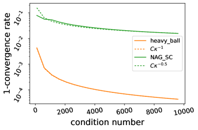
In Euclidean space, Gradient Descent (GD) for -strongly convex and -smooth objective function can converge as 111All the constants in this paper may be different case-by-case, but they are all independent of dimension and the condition number. upon appropriately chosen learning rate. Momentum can accelerate the convergence by softening the dependence on the condition number . However, how momentum is introduced matters to achieving such an acceleration. For example, NAG-SC [16] has convergence rate 222For continuous dynamics, convergence rate means . For discrete algorithms, it means , but Heavy-Ball [18] still has linear dependence on the conditional number, similar to gradient descent without momentum (but it may work better for nonconvex cases).
Remarkable quantitative results also existed for manifold optimization. The momentum-less case is relatively simpler, and [26], for example, developed convergence theory for GD on Riemannian manifold under various assumptions on convexity and smoothness, which matched the classical Euclidean result — for instance, Thm. 15 of their paper gave a convergence rate of 333We will use to denote constants that depend on the manifold structure, e.g., diameter, curvature. It may be different case-by-case. when the learning rate is , under geodesic--strong-convexity and geodesic--smoothness. For the momentum case, [2] analyzed the convergence of a related dynamics in continuous time, namely an optimization ODE corresponding to momentum gradient flow, on Riemannian manifolds under both geodesically strongly and weakly convex potentials, based on a tool of modified cosine rule. However, a convergence analysis for a numerical method in discrete time is still missing. Another series of seminal works include [27, 1], which analyzed the convergence of a class of optimizers by extending Nesterov’s technique of estimating sequence [16] to Riemannian manifolds. They managed to show convergence rate between and , i.e., with conditional number dependence inbetween that of GD with and without momentum in the Euclidean cases. They further proved that, as the iterate gets closer to the minimum, the rate bound gets better because it converges to . However, their algorithm requires the logarithm map (inverse of the exponential map), which may not be uniquely defined on many manifolds (e.g., sphere) and can be computationally expensive. In contrast, Lie NAG-SC, which we will construct, works only for Lie group manifolds, but they are more efficient when applicable, due to being based on only exponential map and gradient oracle. Acceleration of the same type will also be theoretically proved.
Momentum optimizers specializing in Lie groups have also been constructed before [21], where variational optimization [24] was generalized to the manifold setup and then left trivialization were employed to obtain ODEs with Euclidean momentum that perform optimization in continuous time. Our work is also based on those ODEs, whose time however has to be discretized so that an optimization algorithm can be constructed. Delicate discretizations have been proposed in [21] so that the optimization iterates stay exactly on the manifold, saving computational cost and reducing approximation errors. But we will further improve those discretizations. More precisely, note first that [21] slightly abused notation and called both the continuous dynamics and one discretization Lie NAG-SC. However, we find that their splitting discretization may not give the best optimizer – at least, a 1st-order version of their splitting scheme yields a linear condition number dependence in our convergence rate bound. Since this splitting-based optimizer almost degenerates to heavy-ball in the special case of Euclidean spaces (as Rmk. 28 will show), we refine the terminology and call it Lie Heavy-Ball. To remedy the lack of acceleration, we propose a new discretization that actually has square root condition number dependence and thus provable acceleration, and call it as (the true) Lie NAG-SC.
1.2 Main results
We consider the local minimization of a differentiable function , i.e., , where is a finite-dimensional compact Lie group, and the oracle allowed is the differential of .
Two optimizers we focus on are given in Alg. (1). Under assumptions of -smoothness and locally geodesic--strong convexity, we proved that Lie Heavy-Ball has convergence rate , which is approximately the convergence rate of for Lie GD (Eq.1, which is identical to Riemannian GD applied to Lie groups); this is no acceleration. To accelerate, we propose a new Lie NAG-SC algorithm, with provable convergence rate . Note the condition number dependence becomes instead of , hence acceleration.
For a summary our main results, please see Table 1.
Remark 1 (Triviality of convex functions on Lie groups).
We do not assume any global convexity of . In fact, has to be nonconvex for any meaningful optimization to happen. This is because we are considering compact Lie groups444Even if we consider noncompact Lie groups, many of them have compact Lie subgroups [15], and our argument would still hold., and a convex function on a connected compact manifold could only be a constant function [25]. An intuition for this is, a convex function on a closed geodesic must be constant. See [e.g., 13, Sec. B.3] for more discussions. Our analysis is, importantly, for nonconvex , and convexity is only required locally to ensure a quantitative rate estimate can be obtained.
| Continuous dynamics | Heavy-Ball | NAG-SC | |
| Scheme | Eq. (2) | Eq. (9) | Eq. (13) |
| Step size | - | ||
| Convergence rate | |||
| (Modified) energy | Eq. (5) | Eq. (10) | Eq. (41) 555The monotonicity of this energy function requires smaller step size than it listed in this table. See discussion in Rmk. 36 and the details are provided in Sec. D.1 |
| Lyapunov function | Eq. (6) | Eq. (12) | Eq. (14) |
| Main theorem | Thm. 9 | Thm. 13 | Thm. 14 |
2 Preliminaries and setup
2.1 Lie group and Lie algebra
A Lie group, denoted by , is a differentiable manifold with a group structure. A Lie algebra is a vector space with a bilinear, alternating binary operation that satisfies the Jacobi identity, known as Lie bracket. The tangent space at (the identity element of the group) is a Lie algebra, denoted as . The dimension of the Lie group will be denoted by .
Assumption 2 (general geometry).
We assume the Lie group is finite-dimensional and compact.
One technique we will use to handle momentum is called left-trivialization: Left group multiplication is a smooth map from the Lie group to itself and its tangent map is a one-to-one map. As a result, for any , we can represent the vectors in by for . This operation is the left-trivialization. It comes from the group structure and may not exist for a general manifold. If the group is represented via an embedding to matrix group, i.e., , then the left trivialization is simply given by with the right-hand side given by matrix multiplication.
A Riemannian metric is required to take Riemannian gradient and we are considering a left-invariant metric: we first define an inner product on , which is a linear space, and then move it around by the differential of left multiplication, i.e., the inner product at is for , .
2.2 Optimization dynamics
Riemannian GD [e.g., 26] with iteration can be employed to optimize defined on , where is Riemannian gradient, and is the exponential map. To see a connection to the common Euclidean GD, it means we start from and go to the direction of negative gradient with step size to get by geodesic instead of straight line. Riemannian GD can be understood as a time discretization of the Riemannian gradient flow dynamics .
In the Lie group case, it is identical to the following Lie GD obtained from left-trivialization [21]:
| (1) |
where is the left-trivialized gradient. 666The group exponential map and the exponential map from Riemannian structure can be different [13, Sec. D.1]. However, under our choice of the left-invariant metric later in Lemma 3, they are identical and will be the group exponential unless further specified. is the exponential map staring at the group identity following the Riemannian structure given by the left-invariant metric, and the operation between and is the group multiplication. To accelerate its convergence, momentum was introduced to the Riemannian gradient flow via variational optimization and left-trivialization [21], leading to the following dynamics:
| (2) |
Here is the position variable. is the standard ‘momentum’ variable even though it should really be called velocity. It lives , which varies as changes in time, and we will utilize group structure to avoid this complication. More precisely, the dynamics lets the ‘momentum’ be , and is therefore and it is our new, left-trivialized momentum. Intuitively, one can think as angular momentum, and being is position times angular momentum, which is momentum. Similar to the Lie GD Eq. (1), we will not use directly, but its left-trivialization , to update the left-trivialized momentum.
This dynamics essentially models a damped mechanical system, and Tao and Ohsawa [21] proved this ODE converges to a local minimum of using the fact that the total energy (kinetic energy plus potential energy ) is drained by the friction term . In general, can be a positive time-dependent function (e.g., for optimizing convex but not strongly-convex functions), but for simplicity, we will only consider locally strong-convex potentials, and constant is enough.
For curved space, an additional term that vanishes in Euclidean space shows up in Eq. (2). It could be understood as a generalization of Coriolis force that accounts for curved geometry and is needed for free motion. The adjoint operator is defined by . Its dual, known as the coadjoint operator , is given by .
2.3 Property of Lie groups with skew-adjoint
The term in the optimization ODE (2) is a quadratic term and it will make the numerical discretization that will be considered later difficult. Another complication from this term is, it depends on the Riemannian metric, and indicates an inconsistency between the Riemannian structure and the group structure, i.e., the exponential map from the Riemannian structure is different from the exponential map from the group structure. Fortunately, on a compact Lie group, the following lemma shows a special metric on can be chosen to make the term vanish.
Lemma 3 ( skew-adjoint [15]).
Under Assumption 2, there exists an inner product on such that the operator is skew-adjoint, i.e., for any .
This special inner product will also give other properties useful in our technical proofs; see Sec. A.1.
2.4 Assumption on potential function
To show convergence and quantify its rate for the discrete algorithm, some smoothness assumption is needed. We define the -smoothness on a Lie group as the following.
Definition 4 (-smoothness).
A function is -smooth if and only if ,
| (3) |
where is the geodesic distance.
Under the choice of metric in Lemma 3 that is skew-adjoint, Lemma 21 shows this is same as the commonly used geodesic--smoothness (Def. 20).
To provide an explicit convergence rate, some convex assumption on the objective function is usually needed. Under the assumption of unique geodesic on a geodesically convex set , the definition of strongly convex functions in Euclidean spaces can be generalized to Lie groups:
Definition 5 (Locally geodesically strong convexity).
A function is locally geodesic--strongly convex at if and only if there exists a geodesically convex neighbourhood of , denoted by , such that ,
| (4) |
where is well-defined due to the geodesic convexity of .
3 Convergence of the optimization ODE in continuous time
To start, we provide a convergence analysis of the ODE (2), since our numerical scheme comes from its time discretization. We do not claim such convergence analysis for the ODE is new, and in fact, convergence for continuous dynamics has been provided on general manifolds [e.g., 2]. However, we will prove it using our technique to be self-contained and provide some insights for the convergence analysis of the discrete algorithm later.
Define the total energy as
| (5) |
i.e., the total energy is the sum of the potential energy and the kinetic energy. Thanks to the friction , the total energy is monotonely decreasing, which provides global convergence to a stationary point.
Theorem 6 (Monotonely decreasing of total energy [21]).
Suppose the potential function and the trajectory follows ODE (2). Then
Thm. 6 provides the global convergence of ODE (2) to a stationary point under only smoothness: when the system converges, we have , which gives .
Moreover, using the non-increasing property of total energy, the following corollary states that if the particle starts with small initial energy, it will be trapped in a sub-level set of . The local potential well can be defined using ’s sub-level set.
Definition 7 ( sub-level set).
Given , we define the sub-level set of as
i.e. a disjoint union of connected components.
Corollary 8.
Suppose . Let . If the sub-level set of is and , then we have .
Under further assumption of local strong convexity on this sub-level set, convergence rate can be quantified via a Lyapunov analysis inspired by [20]. More specifically, given a fixed local minimum , there is provably a local unique geodesic convex neighbourhood of . Denote it by , and we define on by
| (6) |
By assuming the local geodesic--strong convexity of on , we have the following quantification of Eq. (2).
Theorem 9 (Convergence rate of the optimzation ODE).
If the initial condition satisfies that for some geodesically convex set , is locally geodesic--convex on , and the sub-level set of with satisfies , then we have
| (7) |
with by choosing .
Remark 10.
This theorem alone is a local convergence result and a {Lie group + momentum} extension of an intuitive result for Euclidean gradient flow, which is, if the initial condition is close enough to a minimizer and the objective function has a positive definite Hessian at that minimizer, then gradient flow converges exponentially fast to that minimizer. However, Thm.6 already ensures global convergence, and if not stuck at a saddle point, the dynamics will eventually enter some local potential well. If that potential well is locally strongly convex at its minimizer, then the local convergence result (Thm.9) supersedes the global convergence result (which has no rate), and gives the asymptotic convergence rate. Note however that different initial conditions may lead to convergence to different potential wells (and hence minimizers), as usual.
4 Convergence of Lie Heavy-Ball/splitting discretization in discrete time
One way to obtain a manifold optimization algorithm by time discretization of the ODE (2) is to split its vector field as the sum of two, and use them respectively to generate two ODEs:
| (8) |
Each ODE enjoys the feature that its solution stays exactly on [21], and therefore if one alternatively evolves them for time , the result is a step- time discretization that exactly respects the geometry (no projection needed). If one approximates by , then the same property holds, and the resulting optimizer is
| (9) |
In Euclidean cases, such numerical scheme can be viewed as Polyak’s Heavy-Ball algorithm after a change of variable (Rmk. 27), and will thus be referred to as Lie Heavy-Ball. It is also a 1st-order (in ) version of the ‘2nd-order Lie-NAG’ optimizer in [21] (Rmk. 28).
To analyze Lie Heavy-Ball’s convergence, we again seek some ‘energy’ function such that the iteration of the numerical scheme Eq. (9) will never escape a sub-level set of the potential, similar to the continuous case. Given fixed friction parameter and step size , we define the modified energy as
| (10) |
Theorem 11 (Monotonely decreasing of modified energy of Heavy Ball).
Assume the potential is globally -smooth. When the step size satisfies , we have the modified energy is monotonely decreasing, i.e.,
Thm. 11 provides the global convergence of Heavy-Ball scheme Eq. (9) to a stationary point under only -smoothness: Due to the monotonicity of the energy function , the system will eventually converge. When it converges, since is not moving, we have , leading to the fact that . More importantly, the following corollary shows that the non-increasing property of the modified traps in sub-level set of :
Corollary 12.
Let . If the sub-level set of satisfies and
| (11) |
Then we have for any for the Heavy-Ball scheme Eq. (9) when .
Under further assumption of local strong convexity on this sub-level set, convergence rate can be quantified via a Lyapunov analysis inspired by [20]. More specifically, given a fixed local minimum , there is a local unique geodesic neighbourhood of , denoted by , and we define on by
| (12) |
The exponential decay for the Lyapunov function (Lemma 32) helps us quantify of the convergence rate for Eq. (9) in the following theorem:
Theorem 13 (Convergence rate of Heavy-Ball scheme).
If the initial condition satisfies that for some geodesically convex set , is -smooth and locally geodesic--convex on , and the sub-level set of with satisfies and Eq. (11), then we have
with by choosing , .
Note the rate is . The condition number dependence is linear () but not . Similarly, the procedure of global convergence local potential well local minimum discussed in Rmk. 10 also applies the Heavy-Ball algorithm.
5 Convergence of Lie NAG-SC in discrete time
The motivation for NAG-SC is to improve the condition number dependence. The convergence rate of Heavy-Ball shown in Thm. 13 is the same as the momentumless case [e.g., 26, Thm. 15] under the assumption of local strong convexity and -smoothness. To improve the condition number dependence, inspired by [20], we define Lie NAG-SC as the following:
| (13) |
Comparing to Lie Heavy-Ball, an extra term is introduced (see [20, Sec. 2] for more details in the Euclidean space). Our technique of left-trivialized (and hence Euclidean) momentum allows this trick to transfer directly from Euclidean to the Lie group case.
For NAG-SC, we will only provide a local convergence with quantified convergence under -smoothness and local geodesically convexity on a geodesically convex subset . The difficulty for designing a modified energy and prove the global convergence will be given later in Rmk. 36. We define the following Lyapunov function:
| (14) | |||
where is the minimum of in . This Lyapunov function helps us to trap in a local potential well and quantify the convergence rate:
Theorem 14 (Convergence rate of NAG-SC).
If the initial condition satisfies that for some geodesically convex set satisfying for some and , is -smooth and locally geodesic--convex on , and the sub-level set of with satisfies and
| (15) |
then we have
by choosing and , with .
Unlike sampling ODE and Lie Heavy-Ball, monotonely decreaing modified energy is not provided for Lie NAG-SC. It is unclear whether such modified energy for NAG-SC exists, and an intuition is provided in the Rmk. 36.
Another fact in Thm. 14 that is worth noticing is, we have a term that depends on the curvature of the Lie group 777In comparison, Euclidean NAG-SC has convergence rate [20]., while the Lie Heavy-Ball has the same convergence rate as the Euclidean case [20]. It is unclear if the lost of convergence rate in Lie NAG-SC comparing to the Euclidean case is because of our proof technique or the curved space itself. However, we try to provide some insights in Rmk. 35.
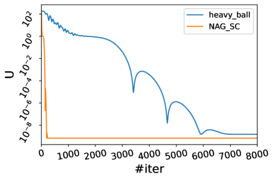
6 Systematic numerical verification via the eigen decomposition problem
6.1 Analytical estimation of property of eigenvalue decomposition potential
Given a symmetric matrix, its eigen decomposition problem can be approached via an optimization problem on :
where . This problem is a hard non-convex problem on manifold, but some analytical estimation [e.g., 6, Thm. 4] can be helpful for us to choose optimizer hyperparameters (we don’t have to have those to apply the optimizers, but in this section we’d like to verify our theoretical bounds and hence and are needed).
This problem is non-convex with stationary points corresponding to the elements in -order symmetric group, including local minima and including local mixima. We suppose with , where ’s (the diagonal values of ) are in ascend order. Given in the -symmetric group, the corresponding local minimum is , i.e., we switch the columns of by . The eigenvalues of its Hessian at the local minimum can be written as
The global minimum is given by with minimum value .
6.2 Numerical Experiment
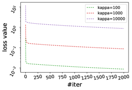
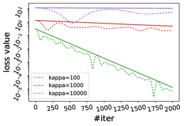
We use the eigenvalues at the global minimum to estimate the and in its neighborhood. As a result, around the global minimum, , and , where we assume ’s are sorted in the ascend order. Such estimation is used to choose our parameters ( and ) in all experiments as stated in Table 1.
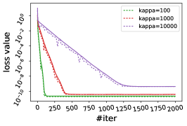
Given a conditional number , we design in the following way: we choose and is uniformly sampled from using [17, Sec. 2.1.1]. When the given satisfies , the condition number at global minimum is the given .
The results are presented in Fig. 1 and 2. In all experiments, we set , and the the computation are done on a MacBook Pro (M1 chip, 8GB memory).
References
- Ahn and Sra [2020] Kwangjun Ahn and Suvrit Sra. From nesterov’s estimate sequence to riemannian acceleration. In Conference on Learning Theory, pages 84–118. PMLR, 2020.
- Alimisis et al. [2020] Foivos Alimisis, Antonio Orvieto, Gary Bécigneul, and Aurelien Lucchi. A continuous-time perspective for modeling acceleration in riemannian optimization. In International Conference on Artificial Intelligence and Statistics, pages 1297–1307. PMLR, 2020.
- Alimisis et al. [2021] Foivos Alimisis, Antonio Orvieto, Gary Becigneul, and Aurelien Lucchi. Momentum improves optimization on riemannian manifolds. In International conference on artificial intelligence and statistics, pages 1351–1359. PMLR, 2021.
- Arjovsky et al. [2016] Martin Arjovsky, Amar Shah, and Yoshua Bengio. Unitary evolution recurrent neural networks. In International conference on machine learning, pages 1120–1128. PMLR, 2016.
- Bonnabel [2013] Silvere Bonnabel. Stochastic gradient descent on riemannian manifolds. IEEE Transactions on Automatic Control, 58(9):2217–2229, 2013.
- Brockett [1989] Roger W Brockett. Least squares matching problems. Linear Algebra and its applications, 122:761–777, 1989.
- Chen et al. [2019] Zhehui Chen, Xingguo Li, Lin Yang, Jarvis Haupt, and Tuo Zhao. On constrained nonconvex stochastic optimization: A case study for generalized eigenvalue decomposition. In The 22nd International Conference on Artificial Intelligence and Statistics, pages 916–925. PMLR, 2019.
- Cisse et al. [2017] Moustapha Cisse, Piotr Bojanowski, Edouard Grave, Yann Dauphin, and Nicolas Usunier. Parseval networks: Improving robustness to adversarial examples. In International conference on machine learning, pages 854–863. PMLR, 2017.
- Dynkin [2000] EB Dynkin. Calculation of the coefficients in the campbell–hausdorff formula. DYNKIN, EB Selected Papers of EB Dynkin with Commentary. Ed. by YUSHKEVICH, AA, pages 31–35, 2000.
- Guigui and Pennec [2021] Nicolas Guigui and Xavier Pennec. A reduced parallel transport equation on lie groups with a left-invariant metric. In Geometric Science of Information: 5th International Conference, GSI 2021, Paris, France, July 21–23, 2021, Proceedings 5, pages 119–126. Springer, 2021.
- Hairer et al. [2006] Ernst Hairer, Marlis Hochbruck, Arieh Iserles, and Christian Lubich. Geometric numerical integration. Oberwolfach Reports, 3(1):805–882, 2006.
- Helfrich et al. [2018] Kyle Helfrich, Devin Willmott, and Qiang Ye. Orthogonal recurrent neural networks with scaled cayley transform. In International Conference on Machine Learning, pages 1969–1978. PMLR, 2018.
- Kong and Tao [2024] Lingkai Kong and Molei Tao. Convergence of kinetic langevin monte carlo on lie groups. COLT, 2024.
- Kong et al. [2023] Lingkai Kong, Yuqing Wang, and Molei Tao. Momentum stiefel optimizer, with applications to suitably-orthogonal attention, and optimal transport. ICLR, 2023.
- Milnor [1976] John Milnor. Curvatures of left invariant metrics on lie groups, 1976.
- Nesterov [2013] Yurii Nesterov. Introductory lectures on convex optimization: A basic course, volume 87. Springer Science & Business Media, 2013.
- O’Hagan [2007] Sean O’Hagan. Uniform sampling methods for various compact spaces. 2007.
- Polyak [1987] Boris T Polyak. Introduction to optimization. 1987.
- Qiu et al. [2023] Zeju Qiu, Weiyang Liu, Haiwen Feng, Yuxuan Xue, Yao Feng, Zhen Liu, Dan Zhang, Adrian Weller, and Bernhard Schölkopf. Controlling text-to-image diffusion by orthogonal finetuning. Advances in Neural Information Processing Systems, 36:79320–79362, 2023.
- Shi et al. [2021] Bin Shi, Simon S Du, Michael I Jordan, and Weijie J Su. Understanding the acceleration phenomenon via high-resolution differential equations. Mathematical Programming, pages 1–70, 2021.
- Tao and Ohsawa [2020] Molei Tao and Tomoki Ohsawa. Variational optimization on lie groups, with examples of leading (generalized) eigenvalue problems. In International Conference on Artificial Intelligence and Statistics, pages 4269–4280. PMLR, 2020.
- Tripuraneni et al. [2018] Nilesh Tripuraneni, Nicolas Flammarion, Francis Bach, and Michael I Jordan. Averaging stochastic gradient descent on riemannian manifolds. In Conference On Learning Theory, pages 650–687. PMLR, 2018.
- Wen and Yin [2013] Zaiwen Wen and Wotao Yin. A feasible method for optimization with orthogonality constraints. Mathematical Programming, 142(1):397–434, 2013.
- Wibisono et al. [2016] Andre Wibisono, Ashia C Wilson, and Michael I Jordan. A variational perspective on accelerated methods in optimization. proceedings of the National Academy of Sciences, 113(47):E7351–E7358, 2016.
- Yau [1974] Shing-Tung Yau. Non-existence of continuous convex functions on certain riemannian manifolds. Mathematische Annalen, 207:269–270, 1974.
- Zhang and Sra [2016] Hongyi Zhang and Suvrit Sra. First-order methods for geodesically convex optimization. In Conference on learning theory, pages 1617–1638. PMLR, 2016.
- Zhang and Sra [2018] Hongyi Zhang and Suvrit Sra. Towards riemannian accelerated gradient methods. arXiv preprint arXiv:1806.02812, 2018.
Appendix A Properties of Lie groups and functions on Lie groups
A.1 More details about compact Lie groups with left-invariant metric
Comparing with the Euclidean space, Lie groups lack of commutativity, i.e., for , and are not necessarily equal. This can also be characterized by the non-trivial Lie bracket . This non-commutativity leads to the fact that . An explicit expression for is given by Dynkin’s formula [9]. Utilizing Dynkin’s formula, we quantify in the following.
Corollary 15 (Differential of logarithm).
If is well defined, then the differential of logarithm on is given by
| (16) |
where the power series is defined as
| (17) |
The vanishment of can also be understood as the group structure and the Riemannian structure are compatible. See [13] for more discussion. Under such assumption, we have the following properties:
Corollary 16.
Suppose we have is skew-adjoint . Then for any and any such that is well-defined, we have
Corollary 17.
When is well-defined and is skew-adjoint , we have
Corollary 18.
Remark 19 (About existence and uniqueness of ).
As the inverse of , the operator may not be uniquely defined globally. However, we are always considering in a unique geodesic subset of the Lie group, where is defined uniquely in such subset of Lie group. Similarly, even if we do not have globally geodesically strongly convex functions, we only require locally strong convexity.
A.2 More details about functions on Lie groups
The commonly used geodesic -smooth on a manifold is given by the following definition [e.g., 26, Def. 5]:
Definition 20 (Geodesically -smooth).
is geodesically -smooth if for any ,
where is the parallel transport from to .
Proof of Lemma 21.
For any , consider the shortest geodesic connecting and and denote . Using the condition is skew-adjoint, we have and is parallel along by checking the condition for parallel transport [10, Thm. 1]:
Corollary 22 (Properties of -smooth functions).
If is -smooth, then for any , we have
| (20) |
Proof of Cor. 22.
We denote the one of the shortest geodesic connecting and as , i.e., with and , for some with . Then
∎
Lemma 23 (Co-coercivity).
If the function is both -smooth and convex on a geodesically convex set , then we have for any ,
| (21) |
Proof of Lemma 23.
By convexity, we have for any , and ,
We sum these two inequalities and have
which tells that
for some linear map with all eigenvalues between 0 and , i.e., for any .
Now, we select the shortest geodesic connection and , defined by , with and . By
we have
∎
Corollary 24.
If the function is both -smooth and convex on a geodesically convex set , then we have for any ,
| (22) |
Proof.
Corollary 25 (Properties of -strongly convex functions).
Suppose is geodesic--strongly convex on a geodesically convex set , then for any ,
| (24) |
Appendix B More details about optimization ODE
Proof of Thm. 6.
By direct calculation,
∎
Lemma 26 (Monotonicity of the Lyapunov function).
Assume is skew-adjoint for any . Suppose there is a geodesically convex set satisfying:
-
•
is geodesic--strongly convex on a geodesically convex set .
-
•
is the minimum of on .
-
•
for all .
-
•
and its differential is well-defined for all .
Then the solution of ODE (2) satisfies
| (25) |
with the convergence rate given by
Appendix C More details about Heavy-Ball discretization
Remark 27 (Polyak’s Heavy ball [18]).
Heavy-ball scheme in the Euclidean space is
where and are positive parameters. We now write it into a position-velocity form. By setting , we have
We perform the change of variables given by , gives
which is the Euclidean version corresponding to Eq. (9).
Remark 28 (Splitting discretization).
The two systems of ODEs in Eq. (8) are both linear and has exact solutions. We will refer to the numerical scheme evolving their exact solution alternatively by splitting discretization. More precisely, this gives us the following numerical scheme:
| (28) |
Eq. (28) is similar to the ‘NAG-SC’ in [21]. The authors provides a second-order approximation to the optimization ODE Eq. (2) by evolving the two ODEs in Eq. (8) in the following way in each step: 1) evolve -ODE for time; 2) evolve -ODE for time; 3) evolve -ODE for time again. Although this zig-zag scheme is higher order of approximation of the optimization ODE comparing to the the splitting approximation mentioned in Rmk. 28, it is still has the same condition number dependence. The reason is, we can take out the first evolution of time for the -system and it becomes identical to the splitting scheme (with a different initial condition.)
| Splitting scheme | Heavy ball | |
|---|---|---|
| velocity | ||
| friction parameter | ||
| step size |
Before we start the theoretical calculation, we mention that update for in Heavy-Ball scheme Eq. (9) can also be written as
| (29) |
which will be helpful later.
Proof of Thm. 11.
Using Eq. (29), we have the following calculation of :
where the second last inequality is the property of -smooth functions given in Eq. 20.
When , we have , and . ∎
Remark 29.
The design of modified energy for Heavy-Ball in Eq. (10) and Thm. 11 is new, and is different from modified potential function in existing works (e.g., [11]). Our modified energy is not designed to let the Hamiltonian system to have higher order of preserving the total energy, but is defined to ensure monotonicity of the modified energy to ensure global convergence of the numerical scheme.
Remark 30.
Proof of Cor. 12.
We prove this by induction. Suppose we have . By the dissipation of the modified energy Thm. 11, . As a reuslt,
Since we have , we have . Together with the condition that , we have . Mathematical induction gives the desired result. ∎
Lemma 31.
Assume is skew-adjoint for any . Suppose there is a geodesically convex set satisfying:
-
•
is geodesically -strongly convex on a convex set .
-
•
is the minima of on .
-
•
for all .
-
•
and its differential is well-defined for all .
Then we have
where is given by
Proof of Lemma 31.
For following the Heavy-Ball scheme Eq. (9), we use the shorthand notation of , which gives
| (30) |
Evaluate of the three terms in separately :
•The first term: By co-coercivity in Lemma 23, we have
•The second term: Using Eq. (29), we have
•The third term: Define a parametric curve as
We evaluate the two terms separately.
Using the update in Eq. (29), we have
Sum them up, we have
Take a closer look:
Now we sum everything up
By Eq. (4) (strong convexity) and Eq. (22) (corollary of co-coercivity) of , we have
| (31) | ||||
Cauchy-Schwarz inequality gives
| (32) |
Lemma 32 (Monotonicity of the Lyapunov function for Heavy-Ball scheme).
Assume the conditions in Lemma 31 is satisfied. By choosing and step size , we have and
| (33) |
by defining .
Appendix D More details about NAG-SC discretization
Lemma 33.
Assume is skew-adjoint for any . Suppose there is a geodesically convex set satisfying:
-
•
is geodesically -strongly convex on a convex set .
-
•
is the minima of on .
-
•
for all .
-
•
and its differential is well-defined for all .
-
•
for some .
Setting and , we have
for the contraction rate given by
| (34) |
Proof of Lemma 33.
For following the NAG-SC scheme Eq. (13), we define the shorthand notation , which gives
| (35) |
Evaluate of the basic terms of first:
•The first term: By the property of convex -smooth functions in Eq. (21),
•The second term: NAG-SC scheme in Eq. 13 gives the following:
•The third term: We consider the parametric curve on connecting and defined by .
First, we estimate the term using the property of in Cor. 16, 17 and 18.
| (36) |
Taking integral gives
We calculate the integral
which gives us
The other term
Summing them up, we have
Eventually, the third term becomes
| extra term from curvature |
We sum the all the terms up to get
| Additional term | |||
| extra term from curvature |
| Additional term | |||
| extra term from curvature |
When , together with Lemma 33 and Cauchy-Schwarz inequality, we have
where is a parameter to be chosen later. Using property of -smoothness in Eq. (21), (22) and property of -strong convexity in Eq. (24), we have for any and satisfying ,
| (37) |
Now we try to upper bound . Using Cauchy-Schwarz inequality,
As a result,
which is same as
| (38) |
We suppose
| (39) |
Now we try to give a lower bound for the contraction rate upon a set of parameters . By assuming , we have
Choosing
to make Eq. (39) satisfied. By assuming , we choose
to make . Then we have
by choosing , same as continuous case and simply choose .
Setting , we have
which gives us the desired result. ∎
Corollary 34.
Proof of Cor. 34.
First we prove . By -smoothness and geodesic convexity, Lemma 23 gives
As a result, when , we have , leading to .
Now we are ready to prove this corollary by induction. Suppose we have . By the monotonicity of the Lyapunov function, . As a result,
Since we have , we have . Together with the condition that , we have . Mathematical induction gives the desired result. ∎
Proof of Thm. 14.
Remark 35 (Why Lie NAG-SC losses convergence rate comparing to the Euclidean case).
In order to utilize the extra term in Eq. (13), Lyapunov function Eq. (14) has the term , and the term needs to be quantified, consequently. However, due to non-linearity of the Lie group, we have to make the assumption that and are close to , leading to the space is ‘nearly linear’, so that we can bound the error from the non-linearity of the space using Cor. 18. Please see the proof of Lemma 33, Eq. (36) for more details.
D.1 Modified energy for NAG-SC
Remark 36 (Why we cannot have an modified energy for NAG-SC).
An ‘modified energy’ for Lie NAG-SC is provided in Eq. (41), whose monotonicity is shown in Thm. 37. The modified energy is global defined and required only -smoothness. However, the failure for this ‘energy function’ is because its monotonicity requires step size , which is smaller than the step size that provides acceleration.
Comparing with the Heavy-Ball scheme, the larger step size and the acceleration of NAG-SC come from extra term , which is closely related to co-coercivity in Lemma 23. However, co-coercivity requires (local) geodesic convexity and -smoothness at the same time, which is not available when we are considering the convergence globally.
The update for in NAG-SC Eq. (13) can be also written as
| (40) |
This inspires us to define the following modified energy:
| (41) |
Theorem 37 (Monotonely decreasing of modified energy of NAG-SC).
Proof of Thm. 37.
Given L-smoothness of , we have
By -smoothness,
Consequently, a sufficient condition for can be given by
By assuming , a sufficient condition for this can be given by , i.e., when
∎