Fate of many-body localization in an Abelian lattice gauge theory

Abstract

We address the fate of many-body localization (MBL) of mid-spectrum eigenstates of a matter-free $U(1)$ quantum-link gauge theory Hamiltonian with random couplings on ladder geometries. We specifically consider an intensive estimator, $\mathcal{D}\in[0,1/4]$, that acts as a measure of elementary plaquettes on the lattice being active or inert in mid-spectrum eigenstates as well as the concentration of these eigenstates in Fock space, with $\mathcal{D}$ being equal to its maximum value of $1/4$ for Fock states in the electric flux basis. We calculate its distribution, $p(\mathcal{D})$, for $L_{x}\times L_{y}$ lattices, with $L_{y}=2$ and $4$, as a function of (a dimensionless) disorder strength $\alpha$ ($\alpha=0$ implies zero disorder) using exact diagonalization on many disorder realizations. Analyzing the skewness of $p(\mathcal{D})$ shows that the finite-size estimate of the critical disorder strength, beyond which MBL sets in for thin ladders with $L_{y}=2$, increases linearly with $L_{x}$ while the behavior of the full distribution with increasing $L_{x}$ at fixed $\alpha$ shows that $\alpha_{c}(L_{y}=2)>40$, if at all finite, based on data for $L_{x}\leq 12$. $p(\mathcal{D})$ for wider ladders with $L_{y}=4$ show their lower tendency to localize, suggesting a lack of MBL in two dimensions. A remarkable observation is the resolution of the (monotonic) infinite temperature autocorrelation function of single plaquette diagonal operators in typical high-energy Fock states into a plethora of emergent timescales of increasing spatio-temporal heterogeneity as the disorder is increased even before MBL sets in. At intermediate and large $\alpha$, but below $\alpha_{c}(L_{y})$, certain randomly selected initial Fock states display striking oscillatory temporal behavior of such plaquette operators dominated by only a few frequencies, reminiscent of oscillations induced by quantum many-body scars.

I Introduction

Interacting many-body lattice models with finite-dimensional local Hilbert spaces are expected to follow the eigenstate thermalization hypothesis (ETH) which states that individual energy eigenstates of such systems have “thermal” expectation values for local observables Deutsch (1991); Srednicki (1994); Rigol et al. (2008); D’Alessio et al. (2016) with the corresponding temperature determined by the energy density of the particular eigenstate. ETH also provides an explanation for how the rest of the system acts as a bath for a subsystem Dymarsky et al. (2018) and causes local equilibration under its own unitary dynamics. It is of great conceptual importance to understand under what conditions ETH might be violated in generic non-integrable systems without the need for fine-tuning to an integrable limit where a macroscopic number of conservation laws emerge Sutherland (2004) that rule out conventional thermalization.

Such a robust mechanism (i.e., stable with respect to small perturbations in the Hamiltonian) is possibly provided by many-body localization (MBL) where, in the presence of sufficiently strong disorder, interacting systems can resist thermalization Basko et al. (2006, 2007); Oganesyan and Huse (2007a); Nandkishore and Huse (2015); Abanin et al. (2019). MBL can be viewed as localization Anderson (1958) of the mid-spectrum eigenstates in a many-body Fock space Macé et al. (2019), where the many-particle Fock states are eigenstates at infinitely strong disorder. On the other hand, ETH posits that such eigenstates should be completely extended in this Fock space. The stability of MBL was argued not to be fine-tuned due to an emergent integrability that arises from the presence of an extensive number of local conservation laws given by operators, dubbed as l-bits, that mutually commute with each other, with these l-bits changing as a function of disorder in the many-body localized phase Serbyn et al. (2013); Huse et al. (2014). The random-field XXZ $S=1/2$ model on finite chains has been the workhorse for MBL Pal and Huse (2010); Luitz et al. (2015) with several unique features characterizing MBL, such as area-law entanglement of mid-spectrum eigenstates, Poisson level statistics of the energy eigenvalues as well as a logarithmic growth of entanglement between two parts of the system with time for quantum quenches from generic unentangled initial states, observed in numerical studies Bauer and Nayak (2013); Serbyn et al. (2013); Žnidarič et al. (2008); Bardarson et al. (2012).

While strong arguments exist in favor of MBL in one dimension Vosk and Altman (2013); Vosk et al. (2015); Pekker et al. (2014); Imbrie (2016a, b) and its absence in higher dimensions De Roeck and Huveneers (2017); Luitz et al. (2017) for short-ranged models, a rigorous proof of the same is still lacking. Numerical studies based on exact diagonalization (ED) have strong drifts in finite-size estimators which makes locating the critical disorder strength of the MBL transition challenging. Techniques that work directly in the thermodynamic limit, such as numerical linked cluster expansion techniques Devakul and Singh (2015), indicate that the MBL phase may be overestimated in ED studies suggesting that currently accessible system sizes may be too small to see a many-body localized phase and instead one might be in a MBL regime which crosses over to a thermal phase on much longer length scales. While some works have suggested the absence of MBL in one dimension Šuntajs et al. (2020), more recent works Crowley and Chandran (2022); Morningstar et al. (2022) argued that much higher disorder may be needed to actually stabilize MBL in the thermodynamic limit.

Recently, thermalization properties of short-ranged interacting models with constrained Hilbert spaces have received a great deal of attention due to the striking observation of persistent many-body revivals in a kinematically-constrained chain of $51$ Rydberg atoms Bernien et al. (2017) when initialized in a Néel state while other high-energy initial states thermalized rapidly, as expected from ETH. A minimal model with a constrained Hilbert space to incorporate strong Rydberg blocking, the PXP model Sachdev et al. (2002); Lesanovsky and Katsura (2012), revealed that this ergodicity-breaking mechanism is due to the presence of some highly-athermal ETH-violating eigenstates Turner et al. (2018a, b), dubbed quantum many-body scars, embedded in a spectrum that satisfies ETH. More recent work on infinite-temperature energy transport shows a novel super-diffusive regime Ljubotina et al. (2023) in PXP chains. It is interesting to ask whether such kinematically-constrained theories can exhibit MBL in the presence of quenched disorder. While studies on disordered PXP chains Chen et al. (2018) as well as on other constrained systems Royen et al. (2024) including disordered quantum dimer models on two-dimensional lattices Théveniaut et al. (2020); Pietracaprina and Alet (2021) suggested the possibility of MBL in such models, an analysis of a family of generalized PXP models with quenched randomness in one-dimensional chains Sierant et al. (2021) gives evidence for the absence of MBL in the thermodynamic limit. In particular, Théveniaut et al. (2020) investigated the same Hamiltonian as here, but in a more constraining superselection sector, while Pietracaprina and Alet (2021) explored the same Hamiltonian on a different lattice. The aim of both investigations was to use constrained Hilbert spaces to maximize the physical sizes for which MBL could be detected. Both investigations concluded the existence of ergodic and localized regimes on lattices involving 64 and 78 sites, and at below and above moderately large disorder strengths. However, no clear transition could be identified.

Constrained Hilbert spaces also arise naturally in Hamiltonian formulations of lattice gauge theories (LGTs) Kogut and Susskind (1975) since physical (gauge-invariant) states satisfy an appropriate Gauss law. In this article, we undertake a systematic study of the nature of the mid-spectrum eigenstates of a particular pure $U(1)$ lattice gauge theory without any dynamical matter as a function of the disorder strength when one of the non-commuting terms in the Hamiltonian is made random. We consider a $U(1)$ quantum link model (QLM) with the gauge degrees of freedom being quantum spins $S=1/2$ Chandrasekharan and Wiese (1997) that live on the links of ladders of a fixed width $L_{y}=2$ or $4$ and length $L_{x}$ and restrict to the Gauss law sector with zero charge at each vertex of the lattice. We consider the most local Hamiltonian in real space, consistent with the Gauss law, where the potential (kinetic) terms are defined on elementary plaquettes and are diagonal (off-diagonal) in the electric flux basis. Quenched disorder is introduced by making the coefficients of the diagonal terms to be random, where the degree of randomness is characterized by a dimensionless parameter, $\alpha$, that equals zero for no randomness and increases monotonically with increasing disorder. To probe MBL, apart from using standard diagnostics like level spacing distributions of the energy eigenvalues, we have considered the probability distribution $p(\mathcal{D})$ of an intensive estimator, $\mathcal{D}\in[0,1/4]$, that simultaneously acts as a measure of elementary plaquettes of the lattice being active or inert in a mid-spectrum eigenstate as well as its spread in Fock space. We also analyze the autocorrelation functions of single plaquette diagonal operators in a given disordered sample starting from typical high-energy Fock states and see evidence of dynamic heterogeneity even before MBL sets in. In particular, the temporal behavior of diagonal plaquette operators in a single disorder realization show striking oscillatory dynamics which are dominated only by a few frequencies from certain randomly selected Fock states whose average energy lies close to the peak of the density of states as a function of energy. However, averaging over Fock states in a single disorder realization to obtain an infinite temperature ensemble result washes out these dynamic heterogeneities. This feature highlights the unusual quantum dynamics present in a disordered kinematically-constrained interacting system even before MBL sets in.

The rest of the article is arranged in the following manner. We define the model and its symmetries in Sec. II. We discuss the level statistics of the energy eigenstates in Sec. III by using data for many disorder realizations as a function of disorder strength and ladder dimensions. We introduce the quantity $\mathcal{D}$ for mid-spectrum eigenstates in Sec. IV, and show how it is related to both the concentration of an eigenstate in Fock space (Sec. IV.1) as well as whether elementary plaquettes in the lattice are active or inert (Sec. IV.2). In Sec. IV.3, we analyze the distribution function, $p(\mathcal{D})$, obtained after using many disorder realizations, as a function of disorder and ladder dimensions which allows us to estimate the disorder strength beyond which MBL is stabilized. We analyze the autocorrelation functions for single plaquette diagonal operators for a given disorder realization in Sec. V as a function of disorder strength. Signatures of thermalization at small disorder are discussed in Sec. V.1 while the emergence of spatio-temporal heterogeneity at intermediate and strong disorder are discussed starting from typical Fock states in Sec. V.2. In particular, certain randomly selected Fock states display oscillatory behavior of these local diagonal operators in time. We finally conclude and discuss some open issues in Sec. VI.

II Disordered U(1) QLM on ladders

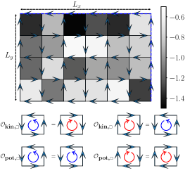
Figure 1: (Top panel) An electric flux configuration for a $L_{x}\times L_{y}=6\times 4$ lattice with periodic boundary conditions in both directions. The shading on the elementary plaquettes denote the different values of $-(1+\alpha R_{\square})$ (see Eq. 1) for one particular disorder realization where $\alpha=1$ and $R_{\square}$ is an independently chosen random number at each plaquette from the uniform distribution $[-1/2,1/2]$. (Bottom panel) Action of $\mathcal{O}_{\mathrm{kin},\square}$ and $\mathcal{O}_{\mathrm{pot},\square}$ shown for elementary flippable plaquettes. Here, clockwise (anti-clockwise) circulation of electric fluxes around a plaquette is marked in red (blue) inside the plaquette.

We consider a disordered $U(1)$ QLM with gauge degrees of freedom being quantum spins $S=1/2$ living on the links $\mathbf{r},\hat{\mu}$ connecting two neighbouring sites $\mathbf{r}$ and $\mathbf{r}+\hat{\mu}$ (where $\hat{\mu}=\hat{i},\hat{j}$) of a ladder whose width equals $L_{y}$ and length equals $L_{x}$ and take periodic boundary conditions in both directions (see Fig. 1, top panel). A $U(1)$ quantum link, $U_{\mathbf{r},\hat{\mu}}=S_{\mathbf{r},\hat{\mu}}^{+}$ is a raising operator of the electric flux $E_{\mathbf{r},\hat{\mu}}=S_{\mathbf{r},\hat{\mu}}^{z}$. We specifically consider even $L_{x}$ and $L_{y}$ with the following Hamiltonian:

$$\mathcal{H}_{\rm dis}=-\sum_{\square}\mathcal{O}_{\mathrm{kin},\square}-\sum_{\square}(1+\alpha R_{\square})\mathcal{O}_{\mathrm{pot},\square}$$ (1)

where each $R_{\square}$ is an independently chosen random number from the uniform distribution $[-1/2,1/2]$ whose specification on all the elementary plaquettes defines a single disorder realization of $\mathcal{H}_{\rm dis}$, $\alpha\geq 0$ and is a dimensionless characterization for the strength of disorder, with $\alpha=0$ ($\alpha\rightarrow\infty$) representing zero (infinite) disorder. The operator $\mathcal{O}_{\mathrm{kin},\square}$ changes the orientation of the electric flux loops around an elementary plaquette from clockwise to anticlockwise and vice versa (Fig. 1, bottom panel), and annihilates non-flippable plaquettes. $\mathcal{O}_{\mathrm{pot},\square}$ is a diagonal counting operator in the electric flux basis, where each flippable (non-flippable) plaquette is counted as $1$ ($0$) (Fig. 1, bottom panel). This Hamiltonian has a local $U(1)$ symmetry generated by the Gauss law $G_{\mathbf{r}}=\sum_{\mu}(E_{\mathbf{r},\hat{\mu}}-E_{\mathbf{r-\hat{\mu}},\hat{\mu}})$. The physical states $|\psi\rangle$ satisfy $G_{\mathbf{r}}|\psi\rangle=0$ which implies that in-coming and out-going electric fluxes add up to zero on each site (see Fig. 1, top panel for an example of such an electric flux configuration), resulting in no background charge at any site, and providing a constrained Hilbert space. The total electric flux winding around the lattice in a given periodic direction is a conserved quantity as well, related to a $U(1)$ center symmetry, and causes the Hilbert space to break up into distinct topological sectors, characterized by a pair of integer winding numbers $(W_{x},W_{y})$. We restrict ourselves to the largest such sector with $(W_{x},W_{y})=(0,0)$.

The model, without any disorder ($\alpha=0$), has a host of discrete symmetries, including translations by one lattice unit in both directions, discrete rotations and reflections, as well as an internal symmetry of charge conjugation which reverses all the electric fluxes. In the presence of disorder ($\alpha\neq 0$), only the internal symmetry survives and the Hilbert space can be block diagonalized into two sectors with an equal number of states, with the charge conjugation quantum number being $C=\pm 1$ using the basis states

$$|F_{i}\rangle_{\pm}=(|F_{i}\rangle\pm C_{E}|F_{i}\rangle)/\sqrt{2},$$ (2)

where $|F_{i}\rangle$ denotes a Fock state in the electric flux basis and $C_{E}|F_{i}\rangle$ denotes another Fock state obtained by reversing all the electric fluxes of $|F_{i}\rangle$.

While an unconstrained Hamiltonian with $S=1/2$ degrees of freedom on the links of a $L_{x}\times L_{y}$ ladder contains $2^{2L_{x}L_{y}}$ configurations, the added local constraint of in- and out-going electric fluxes adding up to zero on each site dramatically decreases the number of allowed states in the Hilbert space (it still scales exponentially in $L_{x}L_{y}$, but with a lower coefficient in the exponent). Furthermore, restricting to the largest topological sector with $(W_{x},W_{y})=(0,0)$ and using the charge conjugation symmetry reduces the allowed number of configurations even further, as shown in Table. 1. For the rest of the article, we present results from ED for $L_{x}\times L_{y}$ ladders with $L_{y}=2$ and $L_{x}=8,10,12$ as well as $6\times 4$ ladders.

Lattice	HSD in $C=\pm 1$ sector for $(W_{x},W_{y})=(0,0)$
$8\times 2$	$1107$
$10\times 2$	$8953$
$12\times 2$	$73789$
$14\times 2$	$616227$
$16\times 2$	$5196627$
$4\times 4$	$495$
$6\times 4$	$16405$
$8\times 4$	$579583$
$6\times 6$	$2741358$

Table 1: Hilbert space dimension (HSD) for different ladders in charge conjugation resolved sector $C=+1/-1$ for the zero winding number topological sector with $(W_{x},W_{y})=(0,0)$.

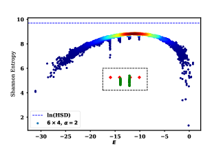
Figure 2: Shannon entropy $S_{1}$ (Eq. 3) for the energy eigenstates of a single disorder realization of a $6\times 4$ lattice with $\alpha=2$. The data for $C=\pm 1$ is shown together in the same plot and the density of states is indicated by a color map where warmer color corresponds to higher density of states. The sublattice scars are shown by a different point font and are enclosed by a box composed of dotted lines for clarity.

The weakly disordered $U(1)$ QLM on ladders is expected to be non-integrable and thus satisfy ETH in the topological sector $(W_{x},W_{y})=(0,0)$ as already discussed in Refs. Banerjee and Sen (2021); Biswas et al. (2022). Since mid-spectrum eigenstates in such a situation are expected to be completely delocalized in Fock space, where the Fock states are defined as in Eq. 2 in the $C=\pm 1$ sector, calculating the Shannon entropy defined as

$$S_{1}(|\Psi\rangle_{\pm})=-\sum_{i}|\psi_{i}|^{2}\ln|\psi_{i}|^{2}$$ (3)

for any eigenstate $|\Psi\rangle_{\pm}=\sum_{i=1}^{\mathrm{HSD}}\psi_{i}|F_{i}\rangle_{\pm}$ (where the subscript $\pm$ denotes the charge conjugation sector) should yield values close to $\ln(\mathrm{HSD})$ for the mid-spectrum eigenstates. In Fig. 2, we see that this expectation is true both for the eigenstates in $C=+1$ and $C=-1$ for a single disorder realization of a $6\times 4$ lattice with $\alpha=2$, though the maximum value of Shannon entropy is somewhat lower than expected of a completely delocalized state Haque et al. (2022). At finite disorder, no two energy eigenstates are expected to be degenerate within these symmetry resolved sectors for any typical disorder realization. The only exception to this statement is provided by certain anomalous eigenstates $|\psi_{\mathrm{sub}}\rangle$, called sublattice scars Sau et al. (2024), that are simultaneous eigenkets of $\sum_{\square}\mathcal{O}_{\mathrm{kin},\square}$ with eigenvalues $0$ or $\pm 2$ as well as of $\mathcal{O}_{\mathrm{pot},\square}$ with eigenvalue $1$ ($0$) on one (the other) sublattice (for even $L_{x},L_{y}$, the lattice is bipartite with elementary plaquettes on one sublattice sharing edges with plaquettes of the other sublattice) with there being a equal number of sublattice scars which have eigenvalue $\mathcal{O}_{\mathrm{pot},\square}=1$ on one sublattice or the other. These sublattice scars are eigenstates of $H$ for any arbitrary $\alpha$ with energies $E_{0,\mathrm{even/odd}}=-\sum_{\square,\mathrm{even/odd}}(1+\alpha R_{\square})$ for the states with eigenvalues $0$ for $\sum_{\square}\mathcal{O}_{\mathrm{kin},\square}$ and $\mathcal{O}_{\mathrm{pot},\square}=1$ for even (odd) sublattice of elementary plaquettes, and with energies $E_{\pm 2,\mathrm{even/odd}}=E_{0,\mathrm{even/odd}}\pm 2$ for the states with eigenvalues $\pm 2$ for $\sum_{\square}\mathcal{O}_{\mathrm{kin},\square}$ and $\mathcal{O}_{\mathrm{pot},\square}=1$ for even (odd) sublattice of elementary plaquettes. For a $6\times 4$ lattice, there are exactly $23$ such sublattice scars with energy $E_{0,\mathrm{even/odd}}$ and $1$ sublattice scar with energy $E_{\pm 2,\mathrm{even/odd}}$ Sau et al. (2024). This degeneracy is clearly reflected in Fig. 2. The anomalous nature of these eigenstates can be seen from the fact that these have significantly lower Shannon entropy than their neighboring eigenstates (Fig. 2). The number of such sublattice scars is, however, a vanishing fraction of the total HSD and does not affect various statistical indicators of ETH versus MBL that we will discuss in Sec. III and Sec. IV. We will, nonetheless, show data for $C=-1$ for $8\times 2$, $C=+1$ for $10\times 2$ and $C=-1$ for $12\times 2$ ladders since these sectors do not have any sublattice scars (compared to $4$ sublattice scars in the other sector) for these ladder dimensions and $C=-1$ for $6\times 4$ ladders since this sector has only $4$ sublattice scars compared to $46$ sublattice scars in $C=+1$ for the same ladder dimension Sau et al. (2024).

III Level spacing distribution

The distribution of energy level spacings in a finite-sized system Oganesyan and Huse (2007b) provides an important diagnostic for whether the model is non-integrable or not, as expected for MBL due to an emergent integrability. Here, we construct the distribution of consecutive level spacing ratios $\tilde{r}\in[0,1]$ of the Hamiltonian $\mathcal{H}_{\mathrm{dis}}$ at finite $\alpha$ after resolving in a sector with $C=+1$ or $C=-1$. The level spacing ratios, $r$, are defined as

$$r=\mathrm{min}\left\{r_{n},\frac{1}{r_{n}}\right\}\leq 1,r_{n}=\frac{s_{n}}{s_{n-1}},s_{n}=E_{n+1}-E_{n},$$ (4)

where $E_{n}$ denotes an energy eigenvalue with $E_{n+1}>E_{n}$. When the model satisfies ETH, one expects the level spacing distribution, $P(r)$, to follow an appropriate Wigner-Dyson distribution (Gaussian orthogonal ensemble (GOE) distribution for the case in hand), while a Poisson distribution is expected for MBL Atas et al. (2013), where:

$$P_{\mathrm{GOE}}(r)=\frac{27}{4}\frac{r+r^{2}}{(1+r+r^{2})^{5/2}};\mbox{~{}~{}}P_{\mathrm{P}}(r)=\frac{2}{(1+r)^{2}}.$$ (5)

The mean level spacing ratio $\langle r\rangle$ also changes from $0.5307(1)$ for the GOE distribution Atas et al. (2013) to $2\ln(2)-1\approx 0.3863$ for the Poisson distribution, thus providing another related means to distinguish between ETH and MBL.

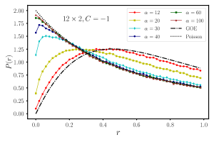
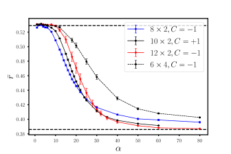
Figure 3: (Top panel) Disorder-averaged distribution $P(r)$ shown for a ladder of dimension $12\times 2$ for various values of $\alpha$. The universal distribution functions $P_{\mathrm{GOE}}(r)$ and $P_{\mathrm{P}}(r)$ (Eq. 5) are also shown for comparison. (Bottom panel) Disorder-averaged mean level spacing $\bar{r}$ shown as a function of disorder strength $\alpha$ for various ladder dimensions. The dotted horizontal lines at $\bar{r}\approx 0.5307$ and $\bar{r}\approx 0.3863$ are the universal values for $P_{\mathrm{GOE}}(r)$ and $P_{\mathrm{P}}(r)$, respectively, and are shown here for comparison.

For the disordered $U(1)$ QLM (Eq. 1), we collect data for many independent disorder realizations ($500$ realizations for $8\times 2$ and $10\times 2$, $50$ realizations for $6\times 4$, $10$ realizations at low disorder and $20$ to $30$ disorder realizations for high disorder for $12\times 2$) at each $\alpha$ to obtain the disorder-averaged distribution $P(r)$ and disorder-averaged mean level spacing $\bar{r}$ (Fig. 3). In Fig. 3 (top panel), we display the results for $P(r)$ as a function of $\alpha$ for $12\times 2$ ladders that have the largest HSD (which equals $73789$) that we could access in our ED studies. While even for $\alpha=12$, $P(r)$ remains close to $P_{\mathrm{GOE}}(r)$, it seems to smoothly crossover to $P_{\mathrm{P}}(r)$ Bogomolny et al. (2001); Buijsman et al. (2019); Sierant and Zakrzewski (2020) as the disorder is increased to $\alpha=100$ suggesting a possible MBL at very large disorder. In Fig. 3 (bottom panel), we show the results for the disorder-averaged mean level spacing $\bar{r}$ for different ladder dimensions as a function of disorder strength $\alpha$. $\bar{r}$ smoothly interpolates from the value expected from a GOE distribution at low $\alpha$ to the one expected from a Poisson distribution at large $\alpha$. The crossing point of these curves for $L_{x}\times 2$ ladders can, in principle, be used to estimate the critical disorder strength, $\alpha_{c}$, needed to stabilize MBL for thin ladders. However, the crossing point shows a drift towards stronger disorder with increasing $L_{x}$ which makes such an estimation difficult. Comparing the disorder-averaged mean level spacing $\bar{r}$ for a wider ladder with dimension $6\times 4$ to that of the $12\times 2$ ladder (Fig. 3 (bottom panel)) clearly shows that a wider ladder, composed of the same number of elementary plaquettes, resists MBL more effectively with increasing disorder.

IV Probing nature of mid-spectrum eigenstates via $\mathcal{D}$

For the disordered $U(1)$ QLM (Eq. 1), the disorder field $(1+\alpha R_{\square})$ couples linearly to the local operator $\mathcal{O}_{\mathrm{pot},\square}$. This suggests that the nature of the mid-spectrum eigenstates may be probed more fruitfully using measures based on the behavior of $\langle\mathcal{O}_{\mathrm{pot},\square}\rangle$ in these eigenstates, where the expectation $\langle\rangle$ is taken with respect to that particular state. For operational reasons, we define the mid-spectrum eigenstates in any particular disorder realization by dividing the bandwidth $(E_{\mathrm{max}}-E_{\mathrm{min}})$, where $E_{\mathrm{max}}$ ($E_{\mathrm{min}}$) refers to the maximum (minimum) energy eigenvalue for that disorder realization, in $25$ equally sized bins and then labelling the states from the bin that contains the maximum number of eigenstates (thus maximizing the density of states as a function of energy) to be mid-spectrum.

For small disorder strength $\alpha\ll 1$ where ETH definitely holds, the form of the Hamiltonian becomes irrelevant for mid-spectrum eigenstates since these locally mimic infinite-temperature thermal states and $\langle\mathcal{O}_{\mathrm{pot},\square}\rangle\rightarrow\langle\mathcal{O}_{\mathrm{pot},\square}\rangle_{\mathrm{th}}$, where $\langle\mathcal{O}_{\mathrm{pot},\square}\rangle_{\mathrm{th}}$ denotes the corresponding infinite-temperature expectation value. For $\alpha\rightarrow\infty$ (infinite disorder limit), the electric flux configurations $|F_{i}\rangle$, as well as $|F_{i}\rangle_{\pm}$ constructed from them (Eq. 2), become eigenstates of $\mathcal{H}_{\mathrm{dis}}$ and thus $\langle\mathcal{O}_{\mathrm{pot},\square}\rangle$ equals $1$ or $0$ in each plaquette for every mid-spectrum eigenstate. Assuming that MBL exists when $\alpha\gg 1$ but finite, we expect $\langle\mathcal{O}_{\mathrm{pot},\square}\rangle$ to typically be pinned close to its extremal values of $0$ or $1$ on each plaquette (since $\mathcal{O}_{\mathrm{pot},\square}$ does not commute with $\mathcal{H}_{\mathrm{dis}}$ for finite $\alpha$, quantum fluctuations make $\langle\mathcal{O}_{\mathrm{pot},\square}\rangle$ deviate from its extreme values) for mid-spectrum eigenstates since this phase should be adiabatically connected Imbrie (2016b) to the infinite disorder point ($\alpha\rightarrow\infty$).

We define the following intensive estimator, $\mathcal{D}\in[0,1/4]$, where $N_{p}$ denotes the total number of elementary plaquettes $L_{x}L_{y}$ for a $L_{x}\times L_{y}$ ladder:

$$\mathcal{D}=\frac{1}{N_{p}}\sum_{\square}\mathcal{D}_{\square}\mbox{~{}~{}}\mathrm{where}\mbox{~{}~{}}\mathcal{D}_{\square}=\left(\langle\mathcal{O}_{\mathrm{pot},\square}\rangle-\frac{1}{2}\right)^{2}.$$ (6)

Assuming ETH, the value of $\mathcal{D}$ for mid-spectrum eigenstates should equal $\mathcal{D}_{\mathrm{th}}$ where $\langle\mathcal{O}_{\mathrm{pot},\square}\rangle_{\mathrm{th}}$ is obtained by using $\mathrm{Trace}[\mathcal{O}_{\mathrm{pot},\square}]/\mathrm{HSD}$ where the trace can be directly carried over the electric flux Fock states in the zero winding number sector that are obtained from direct enumeration. The results for certain ladder dimensions are displayed in Table. 2. In all cases, $\mathcal{D}_{\mathrm{th}}\ll 1$. On the other hand, for $\alpha\rightarrow\infty$, $\mathcal{D}_{\square}\rightarrow 1/4$ from below. In particular, for electric flux Fock states $|F_{i}\rangle$, as well as for basis states of the form $|F_{i}\rangle_{\pm}$ (Eq. 2), $\mathcal{D}=1/4$, as $\mathcal{O}_{\mathrm{pot},\square}$ remains unchanged under charge conjugation.

Lattice	$\langle\mathcal{O}_{\mathrm{pot},\square}\rangle_{\mathrm{th}}$	$\mathcal{D}_{\mathrm{th}}$
$6\times 2$	$0.496454$	$0.0000125$
$8\times 2$	$0.482384$	$0.0003103$
$10\times 2$	$0.474254$	$0.00066286$
$12\times 2$	$0.468986$	$0.000961868$
$14\times 2$	$0.465299$	$0.0012041$
$16\times 2$	$0.462576$	$0.00140056$
$4\times 4$	$0.460606$	$0.00155189$
$6\times 4$	$0.4457$	$0.0029485$
$8\times 4$	$0.438232$	$0.00381529$
$10\times 4$	$0.433827$	$0.0043789$
$6\times 6$	$0.435854$	$0.004115$

Table 2: The values of $\langle\mathcal{O}_{\mathrm{pot},\square}\rangle_{\mathrm{th}}$ and $\mathcal{D}_{\mathrm{th}}$ obtained from direct enumeration of electric flux Fock states in the zero winding numbers sector shown for certain $L_{x}\times L_{y}$ ladders.

IV.1 $\mathcal{D}$ as estimator of concentration of eigenstate in Fock space

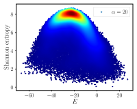
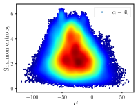
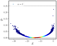
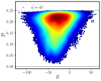
Figure 4: (Top row) Shannon entropy $S_{1}$ (Eq. 3) as a function of energy for all the energy eigenstates of a particular disorder realization for a $12\times 2$ ladder in the $C=-1$ sector at low ($\alpha=2$), intermediate ($\alpha=20$) and large ($\alpha=40$) disorder strengths. The top left panel displays a horizontal dotted line at the value of $\ln(\mathrm{HSD})$ for comparison. (Bottom row) $\mathcal{D}$ (Eq. 6) as a function of energy for all the energy eigenstates for the same system. In all panels, the density of states is indicated by a color map where warmer color corresponds to a higher density of states.

Since $\mathcal{D}_{\mathrm{th}}\ll 1$ while $\mathcal{D}=1/4$ for strictly localized states in the electric flux Fock states, it seems plausible that the value of $\mathcal{D}$ acts as a direct estimator of the concentration of an eigenstate in Fock space. We show numerical evidence that this is indeed the case in Fig. 4 where the top three panels display the Shannon entropy $S_{1}$ for all energy eigenstates in the $C=-1$ sector for one disorder realization of a $12\times 2$ for three different disorder strengths, while the bottom three panels show $\mathcal{D}$ calculated for each eigenstate from the same data sets. The density of states is indicated by the same color map, where warmer colors signify higher density of states, in all the panels. It is clear from the panels in Fig. 4 that $\mathcal{D}$ mirrors the Shannon entropy in all cases, i.e., weak, intermediate and strong disorder, with lower values of $\mathcal{D}$ for the mid-spectrum states implying higher values of $S_{1}$ and, hence, increased delocalization in Fock space.

IV.2 $\mathcal{D}$ as estimator of elementary plaquettes being active/inert in eigenstate

From Table. 2, we see that $\mathcal{D}_{\square}$ acts as a quantifier for whether a plaquette is active or inert in a given mid-spectrum eigenstate since $\mathcal{D}_{\mathrm{th}}\ll 1$ while $\mathcal{D}_{\square}$ should be close to $1/4$ deep in the many-body localized phase. For small $\alpha$, we have verified that $\mathcal{D}_{\square}$ is close to $\mathcal{D}_{\mathrm{th}}$ (apart from finite-size fluctuations) in the mid-spectrum eigenstates, and thus all plaquettes are active as expected.

The behavior of $\mathcal{D}_{\square}$ for different elementary plaquettes of a ladder for mid-spectrum eigenstates is far more interesting for intermediate and large $\alpha$ (see more details in Sec. IV.3). In Fig. 5 and Fig. 6, we display certain chosen mid-spectrum eigenstates from a given disorder realization of a $12\times 2$ ladder and a $6\times 4$ ladder at a large disorder strength of $\alpha=100$. While certain eigenstates indeed have all plaquettes to be inert, there is a hierarchy of thermal regions of varying sizes starting from a few plaquettes all the way up to a system-spanning region of active plaquettes that are connected to each other in other neighboring mid-spectrum eigenstates. We see that mid-spectrum eigenstates that have a bigger number of active plaquettes also have a smaller value of $\mathcal{D}$ at large $\alpha$. Deep inside a many-body localized phase, these thermal regions should be finite and should not scale with system size in any typical mid-spectrum eigenstate to ensure stability of MBL.

While $n$ connected plaquettes, each with a small $\alpha|R_{\square}|$ at large $\alpha$ compared to the bulk, can arise from purely statistical reasons for uniformly distributed random numbers and act as thermal regions because of an effectively smaller disorder locally, the probability of such events scale as $O(1/\alpha^{n})$ and thus decrease very rapidly with increasing $n$ at large $\alpha$. The actual values of $R_{\square}$ for the particular disorder realizations shown in the top panels of both Fig. 5 and Fig. 6 only show certain $n=1$ regions with a low $\alpha|R_{\square}|$ compared to the bulk and rule out this simple interpretation. This already suggests that the large disorder physics of this constrained $U(1)$ QLM may have certain features that are absent in strongly disordered but unconstrained models.

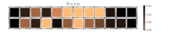
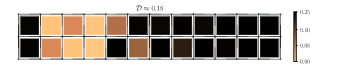
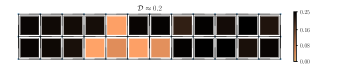
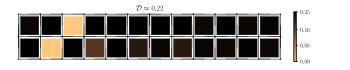
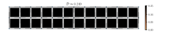
Figure 5: $\mathcal{D}_{\square}$ shown for a few selected mid-spectrum eigenstates from a particular disorder realization for a ladder of $12\times 2$ in the $C=-1$ sector at a large value of disorder, $\alpha=100$. The $R_{\square}$ for each plaquette is specified in the top panel for the particular disorder realization used while in the remaining $6$ panels, darker colors indicate $\mathcal{D}_{\square}$ to be closer to $1/4$ while lighter colors indicate progressively more active plaquettes. For these $6$ panels, the value of $\mathcal{D}$ for the eigenstate is also indicated.

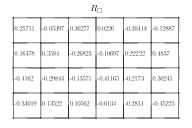
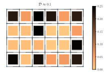
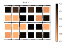
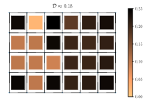
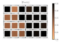
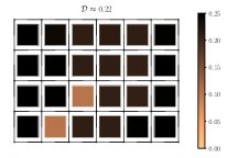
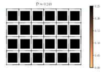
Figure 6: $\mathcal{D}_{\square}$ shown for a few selected mid-spectrum eigenstates from a particular disorder realization for a ladder of $6\times 4$ in the $C=-1$ sector at a large value of disorder, $\alpha=100$. The $R_{\square}$ for each plaquette is specified in the top panel for the particular disorder realization used while in the remaining $6$ panels, darker colors indicate $\mathcal{D}_{\square}$ to be closer to $1/4$ while lighter colors indicate progressively more active plaquettes. For these $6$ panels, the value of $\mathcal{D}$ for the eigenstate is also indicated.

IV.3 Estimating MBL transition using finite-size behavior of $p(\mathcal{D})$

In this section, we will consider the disorder-averaged normalized distribution function, $p(\mathcal{D})$, from ED data for a number of disorder realizations for $8\times 2$, $10\times 2$, $12\times 2$ and $6\times 4$ ladders for various values of $\alpha$. For any given ladder dimension and $\alpha$, we consider several independent disorder realizations and calculate the value of $\mathcal{D}$ for each mid-spectrum eigenstate from that realization. As stated earlier, we divide the total energy bandwidth in $25$ equal bins and choose the bin that contains the maximum number of eigenstates from each disorder realization for this purpose. While we use $500$ disorder realizations for $8\times 2$ and $10\times 2$ ladders and $50$ disorder realizations for $6\times 4$ ladders at each $\alpha$, for the $12\times 2$ ladder with the largest HSD, we use $10$ disorder realizations for $\alpha<20$, $20$ disorder realizations for $\alpha$ between $20$ and $30$ and $30$ disorder realizations for higher values of $\alpha$. The entire dataset for the values of $\mathcal{D}$ for the mid-spectrum eigenstates of all the disorder realizations for a given $L_{x}\times L_{y}$ and $\alpha$ is then divided into $40$ bins to construct the normalized distribution $p(\mathcal{D})$.

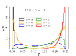
Figure 7: Evolution of $p(\mathcal{D})$ as a function of $\alpha$ for a ladder of dimension $12\times 2$. The y-axis is cut off at $40$ for clarity.

Let us first consider how $p(\mathcal{D})$ is expected to behave when $\alpha\ll 1$ and when $\alpha\gg 1$ (assuming MBL in this case) for fixed ladder widths $L_{y}=2$ or $4$ if $L_{x}\gg 1$. For $\alpha\ll 1$, we expect $p(\mathcal{D})\rightarrow\delta(\mathcal{D}-\mathcal{D}_{\mathrm{th}}(L_{y}))$ where $\mathcal{D}_{\mathrm{th}}(L_{y})$ is expected to be a small number close to $0$ by extrapolating the values given in Table. 2 both for $L_{y}=2$ and $L_{y}=4$. For $\alpha\rightarrow\infty$ (infinite disorder limit), we get $p(\mathcal{D})\rightarrow\delta(1/4-\mathcal{D})$. Assuming adiabatic continuity for $\alpha\gg 1$, which is expected deep in the many-body localized phase (if it exists), $\mathcal{D}$ will decrease from $1/4$ for typical mid-spectrum eigenstates due to perturbatively small quantum fluctuations at large, but finite, $\alpha\gg 1$. Furthermore, since the thermal regions are expected to appear but stay finite in size, deep inside the many-body localized phase for its stability, the intensive estimator $\mathcal{D}$ will only receive sub-dominant ($O(1/L_{x})$) contributions from such active plaquettes when $L_{x}\gg 1$. Thus, $p(\mathcal{D})\rightarrow\delta(1/4-f(\alpha,L_{y})-\mathcal{D})$ where $f(\alpha,L_{y})\ll 1$ assuming that the system is deep in the many-body localized phase from this argument. We will see below that while the finite-size behavior of $p(\mathcal{D})$ indicates a rapid convergence to $\delta(\mathcal{D}-\mathcal{D}_{\mathrm{th}}(L_{y}))$ for a range of $\alpha$ (e.g., see Fig. 8) and an instability towards thermalization with increasing $L_{x}$ for still larger $\alpha$ (e.g., see Fig. 9), the finite-size behavior of $p(\mathcal{D})$ for $\alpha\sim 60-100$ seems more subtle (e.g., see Fig. 10) from data for the available system sizes.

In Fig. 7, we show the behavior of $p(\mathcal{D})$ for a $12\times 2$ ladder as a function of disorder strength $\alpha$. While the distribution has a maximum in the neighborhood of $\mathcal{D}=0$ both for $\alpha=12$ and $\alpha=20$, the tail of the distribution is far more extended at $\alpha=20$ as compared to $\alpha=12$ due to mid-spectrum eigenstates with larger thermally inactive regions becoming more probable at larger $\alpha$. The distribution becomes extremely broad for $\alpha=30$ indicating an instability towards MBL at this system size before developing a pronounced maximum in the neighborhood of $\mathcal{D}=1/4$ for $\alpha\geq 40$. The weight in the tail of the distribution decreases slowly as one increases the disorder from $\alpha=40$ to $\alpha=100$. However, even at a large disorder of $\alpha=100$, there is significant weight in the tail of $p(\mathcal{D})$, consistent with the presence of thermally active regions at various length scales as seen for the mid-spectrum eigenstates in Fig. 5 for one particular disorder realization (as well as for the case of $6\times 4$ ladder, see Fig. 6).

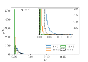
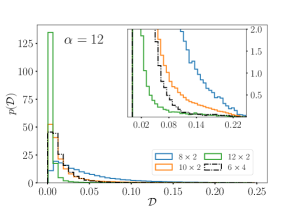
Figure 8: Behavior of $p(\mathcal{D})$ for $8\times 2$, $10\times 2$, $12\times 2$ and $6\times 4$ ladders for $\alpha=6$ (top panel) and $\alpha=12$ (bottom panel). The insets in both panels show the behavior of the tails of $p(\mathcal{D})$ prominently.

To understand whether a ladder of width $L_{y}$ satisfies ETH or demonstrates MBL for a fixed $\alpha$ in the thermodynamic limit of $L_{x}\gg 1$, one needs to compare the behavior of $p(\mathcal{D})$ at that $\alpha$ for different ladder dimensions.

We first consider $\alpha=6$ and $\alpha=12$ as shown in Fig. 8 and focus on $p(\mathcal{D})$ for the $L_{x}\times 2$ ladders. It is clear from both panels in Fig. 8 that the weight in $p(\mathcal{D})$ rapidly shifts to the vicinity of $\mathcal{D}\approx 0$ as a function of increasing $L_{x}$. This is more clearly visible from the inset of both the panels. The insets also show that the tails of the distributions have non-vanishing weights for much larger values of $\mathcal{D}$ at $\alpha=12$ (Fig. 8, bottom panel) compared to $\alpha=6$ (Fig. 8, top panel). This can be interpreted as the emergence of bigger locally inert regions in the mid-spectrum eigenstates as the disorder strength, $\alpha$, is increased from $6$ to $12$. However, the probability of finding such regions with larger inert regions (leading to larger values of $\mathcal{D}$) in mid-spectrum states rapidly decreases with the linear dimension of the ladder, $L_{x}$, as can be seen from the inset of Fig. 8 (bottom panel). It is also interesting to note that for these disorder strengths, a wider ladder of dimension $6\times 4$ has more weight in the tails away from $\mathcal{D}\approx 0$ compared to a $12\times 2$ thin ladder composed of the same number of elementary plaquettes (insets of both panels in Fig. 8) indicating the probability of finding bigger inert regions in typical mid-spectrum eigenstates of the wider ladder.

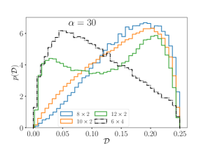
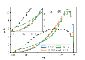
Figure 9: Behavior of $p(\mathcal{D})$ for $8\times 2$, $10\times 2$, $12\times 2$ and $6\times 4$ ladders for $\alpha=30$ (top panel) and $\alpha=40$ (bottom panel). The inset in the bottom panel shows the behavior of the tails of $p(\mathcal{D})$ prominently.

We then look at higher disorder values of $\alpha=30$ (Fig. 9, top panel) and $\alpha=40$ (Fig. 9, bottom panel). For $\alpha=30$, $p(\mathcal{D})$ displays a global maximum in the neighborhood of $\mathcal{D}=1/4$ for $8\times 2$, $10\times 2$ and $12\times 2$ ladders with all three distributions being very broad (Fig. 9, top panel) implying that typical mid-spectrum eigenstates have a significant probability to have large inert regions in real space. However, as the size of a thin ladder with $L_{y}=2$ is increased from $L_{x}=8$ to $L_{x}=12$, we see that the probability to have large active regions in mid-spectrum eigenstates increases, while the weight of the distribution for larger $\mathcal{D}$ (and thus, larger inert regions) decreases. The increase in $p(\mathcal{D})$ for small $\mathcal{D}$ is particularly significant when increasing the ladder dimension from $10\times 2$ to $12\times 2$. This reflects an instability towards thermalization as $L_{x}$ is increased for $\alpha=30$. The same trend is observed for a higher disorder of $\alpha=40$ as well for the thin ladders with $L_{y}=2$ (Fig. 9, bottom panel). Here, $p(\mathcal{D})$ has an even more pronounced maximum in the neighborhood of $\mathcal{D}=1/4$ reflecting that the probability of encountering a large inert region in a typical mid-spectrum eigenstate has increased with disorder. However, focusing on the weight of the distribution for small $\mathcal{D}$ (see inset of Fig. 9, bottom panel for a zoomed version) again shows an instability towards thermalization when $L_{x}$ is increased from $10$ to $12$ due to an increased probability to have larger active regions in real space. While this trend of an increase in $p(\mathcal{D})$ for low $\mathcal{D}$ was already clear when comparing $L_{x}=8$ with $L_{x}=10$ for $\alpha=30$, we see that for higher disorder, this only becomes evident when comparing $p(\mathcal{D})$ for $L_{x}=10$ and $L_{x}=12$ (see inset of Fig. 9, bottom panel) reflecting the increasing length scale needed to probe an instability towards thermalization as the disorder is increased. Comparing $p(\mathcal{D})$ for a $6\times 4$ ladder to that of a $12\times 2$ ladder for these two cases (Fig. 9) clearly shows that the wider ladder is more efficient at resisting MBL due to a much larger value of $p(\mathcal{D})$ at lower $\mathcal{D}$, and hence an enhanced probability of getting large active regions in typical mid-spectrum eigenstates.

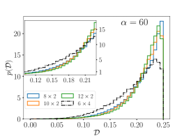
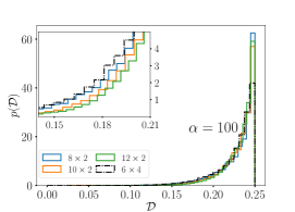
Figure 10: Behavior of $p(\mathcal{D})$ for $8\times 2$, $10\times 2$, $12\times 2$ and $6\times 4$ ladders for $\alpha=60$ (top panel) and $\alpha=100$ (bottom panel). The insets in both panels show the behavior of the tails of $p(\mathcal{D})$ prominently.

We finally show $p(\mathcal{D})$ for even higher disorder, i.e., $\alpha=60$ (Fig. 10, top panel) and $\alpha=100$ (Fig. 10, bottom panel). While both cases show that $p(\mathcal{D})$ has a pronounced maximum at $\mathcal{D}$ close to $1/4$, with the weight being higher at for $\alpha=100$, the weight in the tails away from the maximum (see inset of both panels in Fig. 10) decay very slowly with system size, unlike the case of Fig. 8. with these available sizes, it is not yet clear whether $p(\mathcal{D})$ ultimately converges to $\delta(1/4-f(\alpha,L_{y})-\mathcal{D})$ as the system size is increased (since MBL would imply finite, and not system spanning, active regions in typical mid-spectrum eigenstates) or there is an instability towards thermalization (akin to the case of $\alpha=30$ and $40$) but at larger length scales. Even at these high disorder values, comparing the $p(\mathcal{D})$ data for $6\times 4$ ladder with $12\times 2$ ladder shows that the wider ladder has a higher probability of large active regions in typical mid-spectrum eigenstates (see inset of both panels in Fig. 10). Based on the finite-size behavior of $p(\mathcal{D})$ for thin ladders with $L_{x}=2$, we can conclude that the critical disorder strength, $\alpha_{c}(L_{y}=2)$, for the transition to MBL in the thermodynamic limit is $\alpha_{c}(L_{y}=2)>40$, if at all finite. Furthermore, comparing $p(\mathcal{D})$ of $6\times 4$ ladder with the data for the thin ladders strongly suggests that $\alpha_{c}(L_{y}=4)>\alpha_{c}(L_{y}=2)$.

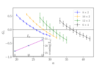
Figure 11: The adjusted Fisher-Pearson coefficient $G_{1}$ (Eq. 7) for the different ladders as a function of $\alpha$. For a given ladder dimension, the skewness coefficient crossing from positive to negative values gives a finite-size estimate $\alpha_{c}(L_{x},L_{y})$. The inset displays the behavior of this estimator for the thin ladders with $L_{y}=2$ as a function of ladder length $L_{x}$ from the available system sizes.

The skewness (which is directly related to the third central moment) of the distribution, $p(\mathcal{D})$, presents another route to calculate a finite-size estimator for the location of the transition from ETH to MBL. The adjusted Fisher-Pearson skewness coefficient is defined Joanes and Gill (1998) for a data set $\{x_{i}\}$ of size $n$ with mean $\bar{x}$ and standard deviation $s$ as follows:

$$G_{1}=\frac{\sqrt{n(n-1)}}{n-2}\frac{\sum_{i=1}^{n}(x_{i}-\bar{x})^{3}/n}{s^{3}}.$$ (7)

and measures the asymmetry of the distribution around its mean. E.g., if we consider the evolution of $p(\mathcal{D})$ for a $12\times 2$ ladder as a function of disorder $\alpha$ (Fig. 7), we see that at low (high) $\alpha$, the distribution has a tail towards higher (lower) values of $\mathcal{D}$ resulting in a positive (negative) $G_{1}$. The skewness coefficient crosses $0$ around $\alpha\sim 30$ where the distribution becomes broad and symmetric. Thus, the value of $\alpha$ for which $G_{1}$ crosses from being positive to negative can be taken as a finite-size estimator of $\alpha_{c}$ for a given ladder $L_{x}\times L_{y}$. We compute $G_{1}$ from the mid-spectrum eigenstates of each disorder realization using Eq. 7 and then use the independent disorder realizations for a given $L_{x}\times L_{y}$ ladder and $\alpha$ to compute its average and error bar. We use $500$ disorder realizations each for $8\times 2$ and $10\times 2$ ladders, $50$ realizations each for $6\times 4$ ladders and $30$ realizations each for $12\times 2$ ladders. The result of such an analysis is displayed in Fig. 11 from which a finite-size estimator $\alpha_{c}(L_{x},L_{y})$ can be directly computed. The inset of Fig. 11 shows that $\alpha_{c}(L_{x},L_{y}=2)$ diverges linearly with $L_{x}$ based on the data for $L_{x}=8,10,12$. Whether this trend continues (which would imply absence of MBL in the thermodynamic limit) or $\alpha_{c}(L_{x},L_{y}=2)$ eventually saturates to a finite value requires data for bigger system sizes. The $G_{1}$ data for the $6\times 4$ ladder in Fig. 11 clearly shows that the wider ladder with $L_{y}=4$ localizes at a larger disorder strength compared to the thin ladders.

V Autocorrelation functions for single plaquette diagonal operators

In this section, we focus on the dynamical properties of the disordered $U(1)$ QLM on ladders and particularly consider a range of disorder strengths, $\alpha$, such that it is less than $\alpha_{c}(L_{y})$ (see previous section for estimates of the critical disorder strength to stabilize MBL). While interesting dynamical features including subdiffusion Bar Lev et al. (2015); Gopalakrishnan et al. (2016) have been discussed in thermal systems near a MBL transition, here we probe the autocorrelation functions of the simplest local diagonal operators $\mathcal{O}_{\mathrm{pot},\square}$ for individual disorder realizations for a given $\alpha$ and ladder dimension for this purpose. Since $\alpha_{c}(L_{y})$ is large (if at all finite) for both $L_{y}=2$ and $L_{y}=4$, the disordered QLM provides us with a setting where the local relaxation of a strongly disordered, yet thermal, system may be studied.

We calculate both the infinite temperature autocorrelation functions as well as autocorrelations starting from typical Fock states whose average energy lies in the bin (of width $4\%$ of the total bandwidth as used in Sec. IV.3 to define mid-spectrum eigenstates) that contains the maximum density of states. Somewhat paradoxically, the infinite temperature autocorrelations are featureless and decay monotonically with time both at low and large disorder. However, the autocorrelations from individual Fock states show more structure. While the dynamics at low disorder shows rapid thermalization and negligible dynamic heterogeneity, the situation is different for intermediate and large disorder where interesting spatio-temporal structures emerge in local relaxation starting from randomly sampled typical Fock states.

We define the autocorrelation functions as follows. Starting from a charge-resolved Fock state $|F\rangle$ (either in the sector $C=+1$ or $C=-1$ using Eq. 2), the local autocorrelation functions on individual plaquettes in a given disorder realization are defined as

$$C_{\square}(|F\rangle,t)=\langle F|\mathcal{O}_{\mathrm{pot},\square}(t)\mathcal{O}_{\mathrm{pot},\square}(0)|F\rangle$$ (8)

where $\mathcal{O}_{\mathrm{pot},\square}(t)=\exp(+i\mathcal{H}_{\mathrm{dis}}t)\mathcal{O}_{\mathrm{pot},\square}\exp(-i\mathcal{H}_{\mathrm{dis}}t)$, from which an average (over space) temporal autocorrelation can be defined as

$$C(|F\rangle,t)=\frac{1}{N_{p}}\sum_{\square}C_{\square}(|F\rangle,t).$$ (9)

An infinite temperature temporal autocorrelation function, that represents the average of $C(|F\rangle,t)$ over all the charge-resolved Fock states, is similarly defined as follows:

$$C_{\mathrm{inf}}(t)=\frac{1}{\mathrm{HSD}}\frac{1}{N_{p}}\sum_{\square}\mathrm{Trace}[\mathcal{O}_{\mathrm{pot},\square}(t)\mathcal{O}_{\mathrm{pot},\square}(0)].$$ (10)

It is useful to note that

$$C_{\square}(|F\rangle,t)=\delta_{\mathcal{O}_{\mathrm{pot},\square},1}\langle\mathcal{O}_{\mathrm{pot},\square}(t)\rangle$$ (11)

by using the fact that $\mathcal{O}_{\mathrm{pot},\square}|F\rangle=\delta_{\mathcal{O}_{\mathrm{pot},\square},1}|F\rangle$ in Eq. 8, where $\delta_{\mathcal{O}_{\mathrm{pot},\square},1}$ is a Kronecker delta function. Thus, $C_{\square}(|F\rangle,t)$ directly probes the temporal evolution of $\langle\mathcal{O}_{\mathrm{pot},\square}\rangle$ and its convergence (or, lack of it) to $\langle\mathcal{O}_{\mathrm{pot},\square}\rangle_{\mathrm{th}}$ (Table 2) as time increases for elementary plaquettes that have a flippable configuration of electric fluxes at $t=0$.

We also define the following normalized autocorrelators [which approach $1$ ($0$) for $t\rightarrow 0$ ($t\rightarrow\infty$)], $\tilde{C}(|F\rangle,t)$ and $\tilde{C}_{\mathrm{inf}}(t)$:

$$\tilde{C}(|F\rangle,t)=\frac{C(|F\rangle,t)-\overline{C(|F\rangle)}_{\infty}}{C(|F\rangle,0)-\overline{C(|F\rangle)}_{\infty}}$$ (12)

and

$$\tilde{C}_{\mathrm{inf}}(t)=\frac{C_{\mathrm{inf}}(t)-\overline{(C_{\mathrm{inf}})}_{\infty}}{C_{\mathrm{inf}}(0)-\overline{(C_{\mathrm{inf}})}_{\infty}}$$ (13)

where $\overline{C(|F\rangle)}_{\infty}$ and $\overline{(C_{\mathrm{inf}})}_{\infty}$ represent infinite-time averages of $C(|F\rangle,t)$ and $C_{\mathrm{inf}}(t)$ in the time range $t\in[0,\infty)$ and have the following expressions:

$$\overline{C(|F\rangle)}_{\infty} = \frac{1}{N_{p}}\sum_{\square}\sum_{m}|\alpha^{m}_{F}|^{2}\langle\Psi_{m}|\mathcal{O}_{\mathrm{pot},\square}|\Psi_{m}\rangle\langle F|\mathcal{O}_{\mathrm{pot},\square}|F\rangle$$

$$\overline{(C_{\mathrm{inf}})}_{\infty} = \frac{1}{\mathrm{HSD}}\frac{1}{N_{p}}\sum_{\square}\sum_{m}|\langle\Psi_{m}|\mathcal{O}_{\mathrm{pot},\square}|\Psi_{m}\rangle|^{2}$$ (14)

with $|F\rangle=\sum_{m}\alpha_{F}^{m}|\Psi_{m}\rangle$ where $|\Psi_{m}\rangle$ represents the $m$-th eigenstate of $\mathcal{H}_{\mathrm{dis}}$ for a given disorder realization in the sector $C=\pm 1$.

In this section, we will show results for such autocorrelations for disorder strengths $\alpha=6,12,30$ for a $10\times 2$ ladder as well as for $\alpha=6,30$ for a wider ladder of dimension $6\times 4$ for a particular disorder realization (i.e., specification of the random numbers $R_{\square}$). While $\alpha=6$ can be treated as ”weak” disorder in both cases, the dynamics at $\alpha=12$ for the thin ladder shows coherent oscillations for the local autocorrelation function $C_{\square}(|F\rangle,t)$ in some elementary plaquettes at intermediate disorder strength (which is still small compared to $\alpha_{c}(L_{y}=2)$) in a small fraction of the randomly chosen Fock states. We will finally discuss the case of strong disorder ($\alpha=30$) for both thin and wide ladders where this fraction of Fock states that show coherent oscillations of the diagonal local operator in some plaquettes becomes much more significant. Additionally, these oscillations point to the emergence of a plethora of time scales at strong disorder. We note that though $\alpha=30$ is a large disorder strength (since $\alpha$ is dimensionless), it is still smaller than both $\alpha_{c}(L_{y}=2)$ and $\alpha_{c}(L_{y}=4)$. These prominent dynamical features at $\alpha=12$ and $\alpha=30$ will be shown to be present in other disorder realizations as well in appendix A. In all the cases, we choose $50$ randomly selected charge-resolved Fock states from the ones whose average energy lies in the bin (with a width of $4\%$ of the total bandwidth) with the highest number of energy eigenstates for the given disorder realization.

V.1 Autocorrelation functions deep in the thermalizing regime

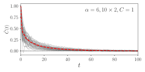
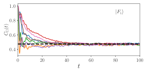
Figure 12: (Top panel) Normalized autocorrelation functions (see Eq. 12 and Eq. 13) shown for the infinite temperature autocorrelation (dashed red curve) as well as the average autocorrelation function starting from $50$ randomly chosen Fock states (shown in grey) with average energies that lie in the bin of width $4\%$ of the total bandwidth and contains the maximum number of eigenstates for a single disorder realization of a $10\times 2$ ladder for $\alpha=6$. (Bottom panel) The local autocorrelation $C_{\square}(|F\rangle,t)$ (Eq. 8) shown for one particular Fock state selected from the top panel. The autocorrelation functions for the different elementary plaquattes are shown using different colors. The horizontal dashed line indicates the value of $\langle\mathcal{O}_{\mathrm{pot},\square}\rangle_{\mathrm{th}}$ for a $10\times 2$ ladder (Table  2).

We first monitor the behavior of the autocorrelations for a disorder strength of $\alpha=6$ for both $10\times 2$ as well as $6\times 4$ ladders. We focus on a single disorder realization in both cases and calculate the normalized versions of the infinite temperature autocorrelation (Eq. 13) as well as the normalized average temporal autocorrelation (Eq. 12) starting from $50$ randomly selected charge-resolved Fock states. The results are displayed in the top panel of Fig. 12 for a $10\times 2$ ladder and the top panel of Fig. 13 for a $6\times 4$ ladder. Both the (normalized) infinite temperature autocorrelations as well as the ones starting from randomly sampled Fock states relax to $0$ as a function of time $t$ reflecting the approach of the diagonal plaquette operators to their final late-time values. The infinite temperature autocorrelation in both cases decay monotonically with $t$; however, the autocorrelation starting from the individual Fock states are not necessarily monotonic at all times, especially at early times. There is a spread of the normalized autocorrelation functions for individual Fock states around the infinite temperature result due to the finite disorder present ($\alpha=6$), with some autocorrelations decaying slower (faster) than the infinite temperature result. However, all the normalized autocorrelations decay to nearly zero beyond a time scale of $t\sim 60$ ($t\sim 80$) for the $10\times 2$ ($6\times 4$) ladder.

It is also instructive to look at $C_{\square}(|F\rangle,t)$ (Eq. 8) for the individual Fock states to probe the local thermalization of $\langle\mathcal{O}_{\mathrm{pot},\square}(t)\rangle$ directly (see Eq. 11). Since the problem is disordered, different regions in space can have different relaxational timescales. We look at one particular Fock state from the $50$ randomly selected Fock states in the lower panel of Fig. 12 (Fig. 13) for $10\times 2$ ($6\times 4$) ladder. It is clear from both figures that while the transients differ for each plaquette due to their different local environments, all the $C_{\square}(t)$ curves saturate close to a steady state value after a time scale of $t\sim 40$ in both cases for the chosen Fock states. Furthermore, the steady state values are close to $\langle\mathcal{O}_{\mathrm{pot},\square}\rangle_{\mathrm{th}}$ (indicated by a horizontal dotted line in the lower panel of Fig. 12 and Fig. 13) for different elementary plaquettes for the corresponding ladder dimension in both the cases. We have checked that this picture remains qualitatively true for the other Fock states shown in the top panel of Fig. 12 and Fig. 13.

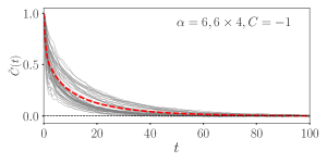
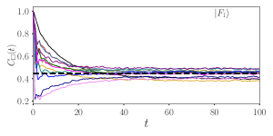
Figure 13: (Top panel) Normalized autocorrelation functions (see Eq. 12 and Eq. 13) shown for the infinite temperature autocorrelation (dashed red curve) as well as the average autocorrelation function starting from $50$ randomly chosen Fock states (shown in gray) with average energies that lie in the bin of width $4\%$ of the total bandwidth and contains the maximum number of eigenstates for a single disorder realization of a $6\times 4$ ladder for $\alpha=6$. (Bottom panel) The local autocorrelation $C_{\square}(|F\rangle,t)$ (Eq. 8) shown for one particular Fock state selected from the top panel. The autocorrelation functions for the different elementary plaquettes are shown using different colors. The horizontal dashed line indicates the value of $\langle\mathcal{O}_{\mathrm{pot},\square}\rangle_{\mathrm{th}}$ for a $6\times 4$ ladder (Table  2).

V.2 Dynamic heterogeneity at intermediate and strong disorder

Let us now consider the nature of the autocorrelation functions for an intermediate disorder strength of $\alpha=12$ for a $10\times 2$ ladder in a single disorder realization. This value of $\alpha$ is still much lower than $\alpha_{c}(L_{y}=2)$ based on our estimates in Sec. IV.3. From Fig. 14 (top panel), we see that while the infinite temperature autocorrelation is still monotonically decaying in time, the average autocorrelation functions from $50$ randomly chosen Fock states shows a bigger spread around the infinite temperature autocorrelation with a few Fock states ($3$ out of $50$ for this particular realization) displaying clear oscillatory behavior (one such autocorrelation curve is indicated in blue for clarity in Fig. 14 (top panel). In Fig. 14 (middle panel), we show the typical behavior of these Fock states by choosing one of the selected Fock states and displaying the local autocorrelation function, $C_{\square}(|F\rangle,t)$, for its plaquettes. While the individual plaquette operators do seem to attain steady state values after a timescale that is longer than compared to the case of $\alpha=6$, the steady state values show a much bigger spread (compared to $\alpha=6$) around the expected result of $\langle\mathcal{O}_{\mathrm{pot},\square}\rangle_{\mathrm{th}}$ from ETH.

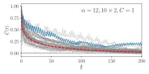
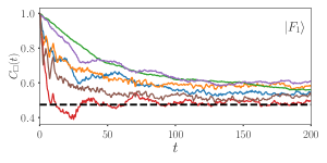
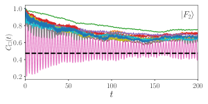
Figure 14: (Top panel) Normalized autocorrelation functions (see Eq. 12 and Eq. 13) shown for the infinite temperature autocorrelation (dashed red curve) as well as the average autocorrelation function starting from $50$ randomly chosen Fock states (shown in grey) with average energies that lie in the bin of width $4\%$ of the total bandwidth and contains the maximum number of eigenstates for a single disorder realization of a $10\times 2$ ladder for $\alpha=12$. One Fock state that shows an oscillatory behavior of the average autocorrelation is marked in blue for clarity. The local autocorrelation $C_{\square}(|F\rangle,t)$ (Eq. 8) shown for one particular Fock state that does not (does) have an oscillatory average autocorrelation selected from the top panel and shown in the middle (bottom) panel. The autocorrelation functions for the different elementary plaquattes are shown using different colors in the middle and bottom panels. The horizontal dashed line in the middle and bottom panels indicates the value of $\langle\mathcal{O}_{\mathrm{pot},\square}\rangle_{\mathrm{th}}$ for a $10\times 2$ ladder (Table  2).

However, the behaviour for the $3$ Fock states with oscillatory average autocorrelations in markedly different. We display the local autocorrelation, $C_{\square}(|F\rangle,t)$, for one such Fock state in Fig. 14 (bottom panel). While several plaquettes approach their steady state values at a timescale comparable to the time scales for the other typical Fock states, these values are very different from the one expected from ETH. Furthermore, some plaquettes show clear coherent oscillations with a slowly decaying envelope (at least till $t=200$) for the diagonal operator $\langle\mathcal{O}_{\mathrm{pot},\square}\rangle$, in stark contrast to expectation from ETH. Here, it is useful to note that $C_{\square}(|F\rangle,t)=0$ for all $t$ of plaquettes that have $\mathcal{O}_{\mathrm{pot},\square}=0$ at $t=0$ in the starting Fock state. However, this does not preclude oscillations in a subset of such elementary plaquettes as well when $\langle\mathcal{O}_{\mathrm{pot},\square}(t)\rangle$ is calculated for such plaquettes and we, indeed, find that to be the case for Fock states whose average autocorrelators show oscillatory behavior.

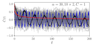
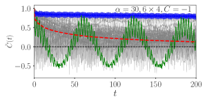
Figure 15: Normalized autocorrelation functions (see Eq. 12 and Eq. 13) shown for the infinite temperature autocorrelation (dashed red curve in both panels) as well as the average autocorrelation function starting from $50$ randomly chosen Fock states (shown in grey) with average energies that lie in the bin of width $4\%$ of the total bandwidth and contains the maximum number of eigenstates for a single disorder realization of a $10\times 2$ ladder (top panel) and a $6\times 4$ ladder (bottom panel) for a disorder strength of $\alpha=30$. Some Fock states that show an oscillatory behavior of the average autocorrelation are marked in different colors in both panels for clarity.

The fraction of these randomly chosen Fock states with oscillatory, instead of decaying, average temporal autocorrelations as well as the dynamic heterogeneity increases significantly as one cranks up the disorder strength even further. We now show results for a disorder strength of $\alpha=30$, both for $10\times 2$ and $6\times 4$ ladders. The increased dynamic heterogeneity is already evident when one calculates the infinite temperature autocorrelation and compares it to the average autocorrelation from $50$ randomly chosen Fock states whose average energies lie within the bin with the highest number of energy eigenstates (Fig. 15). While the infinite temperature autocorrelation is still quite featureless and decays monotonically for both the ladders, we see that the randomly chosen Fock states show a very wide range of dynamical behavior. In particular, there are now $23$ ($14$) Fock states with clear oscillatory dynamics in the average autocorrelation for the particular disorder realization used for $10\times 2$ ($6\times 4$) ladder to generate Fig. 15. Some of these autocorrelations are marked using a different color for clarity in the same figure.

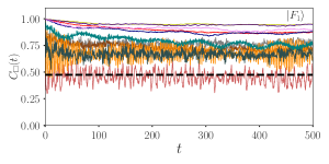
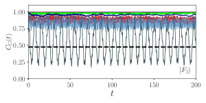
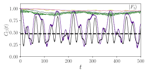
Figure 16: The local autocorrelation $C_{\square}(|F\rangle,t)$ (Eq. 8) shown for three particular Fock states for a $10\times 2$ ladder with $\alpha=30$. The top (middle and bottom) panel displays the local autocorrelation for a Fock state that does not (does) have an oscillatory average autocorrelation. The autocorrelation functions for the different elementary plaquettes are shown using different colors in all panels. The horizontal dashed line in all panels indicates the value of $\langle\mathcal{O}_{\mathrm{pot},\square}\rangle_{\mathrm{th}}$ for a $10\times 2$ ladder (Table  2).

In Fig. 16 (Fig. 17), we show the local autocorrelation of a few selected Fock states from the $50$ randomly chosen Fock states for $10\times 2$ ($6\times 4$) ladder with disorder $\alpha=30$. The top panel of Fig. 16 (Fig. 17) shows an example of a Fock state whose average autocorrelator does not show any significant oscillations for the $10\times 2$ ($6\times 4$) ladder. While $C_{\square}(|F\rangle,t)$ does seem to relax to steady state values for the different plaquettes for the $6\times 4$ ladder, these values are very different from the expected $\langle\mathcal{O}_{\mathrm{pot},\square}\rangle_{\mathrm{th}}$ value for this ladder dimension with most of the plaquettes that start with $\mathcal{O}_{\mathrm{pot},\square}=1$ at $t=0$ giving $\langle\mathcal{O}_{\mathrm{pot},\square}(t)\rangle\geq 0.75$ even for $t\sim 300$. The situation is similar for the autocorrelation of the chosen Fock state in the $10\times 2$ ladder, except that the fluctuations around the steady state of $\langle\mathcal{O}_{\mathrm{pot},\square}\rangle$ for the different plaquettes seems to be larger in this case.

The middle and bottom panels of Fig. 16 (Fig. 17) show examples of the local autocorrelation, $C_{\square}(|F\rangle,t)$, for the different elementary plaquettes for two different Fock states from the $50$ randomly chosen Fock states starting from which the average correlation shows oscillatory behavior in time for a $10\times 2$ ($6\times 4$) ladder. Some of the elementary plaquettes again show persistent oscillations in $\langle\mathcal{O}_{\mathrm{pot},\square}(t)\rangle$ as a function of time. Not only do the different Fock states display different types of temporal behaviors for the same disorder realization, but even the same Fock state can contain elementary plaquettes that show persistent oscillations that involve different sets of frequencies as is clear from the bottom panels of Fig. 16 and Fig. 17.

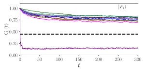
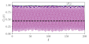
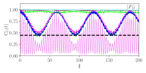
Figure 17: The local autocorrelation $C_{\square}(|F\rangle,t)$ (Eq. 8) shown for three particular Fock states for a $6\times 4$ ladder with $\alpha=30$. The top (middle and bottom) panel displays the local autocorrelation for a Fock state that does not (does) have an oscillatory average autocorrelation. The autocorrelation functions for the different elementary plaquettes are shown using different colors in all panels. The horizontal dashed line in all panels indicates the value of $\langle\mathcal{O}_{\mathrm{pot},\square}\rangle_{\mathrm{th}}$ for a $6\times 4$ ladder (Table  2).

VI Conclusions and outlook

In conclusion, we have considered a $U(1)$ quantum link gauge theory Hamiltonian in its $S=1/2$ representation on $L_{x}\times L_{y}$ ladders, where both $L_{x}$ and $L_{y}$ are taken to be even, with periodic boundary conditions in both directions. This allows us to target the largest superselection sector of such a theory with zero charge at each site and zero winding of electric fluxes in both directions. The Hamiltonian $\mathcal{H}_{\mathrm{dis}}$ (Eq. 1) is composed of plaquette operators, $\mathcal{O}_{\mathrm{kin},\square}$ and $\mathcal{O}_{\mathrm{pot},\square}$, that are defined on the elementary plaquettes of the lattice. While $\mathcal{O}_{\mathrm{kin},\square}$ is off-diagonal in the electric flux basis and changes a clockwise circulation of electric fluxes on a plaquette to anticlockwise and vice versa, $\mathcal{O}_{\mathrm{pot},\square}$ is diagonal and counts whether a plaquette is flippable. We introduce a disorder field that couples linearly to $\mathcal{O}_{\mathrm{pot},\square}$ and parameterize the strength of the disorder by a dimensionless number $\alpha$ where $\alpha=0$ ($\alpha\rightarrow\infty$) represents no (infinite) disorder. We study the properties of mid-spectrum energy eigenstates of this disordered lattice gauge theory to understand whether such a system exhibits a many-body localized phase or not, both on thin ladders with $L_{y}=2$ and wider ladders with $L_{y}=4$, using exact diagonalization techniques. While this specific model is known to be non-integrable for weak disorder, the nature of the mid-spectrum eigenstates for larger disorders has not been explored previously.

In this work, apart from using standard diagnostics like level spacing distributions, we introduce an intensive estimator, $\mathcal{D}=(1/N_{p})\sum_{\square}\mathcal{D}_{\square}\in[0,1/4]$, whose normalized probability distribution $p(\mathcal{D})$ is calculated for mid-spectrum eigenstates using many disorder realizations for a given disorder strength $\alpha$ and ladder dimension. This estimator serves the dual purpose of quantifying how localized a mid-spectrum eigenstate is in Fock space (defined by the electric flux Fock states) as well as estimating the fraction of elementary plaquettes in an active (thermal) or an inactive (inert) state. This is because while $\langle\mathcal{D}_{\square}\rangle=(\langle\mathcal{O}_{\mathrm{pot},\square}\rangle-1/2)^{2}$ is $1/4$ for plaquettes in perfectly localized (in Fock space) electric flux Fock states that become eigenstates at infinite disorder, its infinite-temperature value, $\mathcal{D}_{\mathrm{th}}\ll 1/4$, from explicit calculations which should hold for delocalized (in Fock space) mid-spectrum eigenstates from the eigenstate thermalization hypothesis. The distribution $p(\mathcal{D})$ has a pronounced maximum near $0$ ($1/4$) for small (large) $\alpha$ with a tail whose weight decreases at large (small) $\mathcal{D}$. The analysis of the finite-size behavior of $p(\mathcal{D})$ with increasing $L_{x}$ for thin ladders with $L_{y}=2$ for fixed disorder strengths indicates three regimes: weak disorder with a pronounced maximum near $\mathcal{D}=0$ where the weight in the tails away from the maximum rapidly decrease with increasing system size, intermediate disorder where there is no pronounced maximum near $\mathcal{D}=0$ at the available system sizes but finite-size scaling indicates an instability towards thermalization due to the probability of low $\mathcal{D}$ values increasing with increasing $L_{x}$, and finally strong disorder where the distribution has a pronounced maximum near $\mathcal{D}=1/4$ but the weight in the tails away from the maximum decreases very slowly with system size. Analysis of $p(\mathcal{D})$ for $L_{x}=8,10,12$ for thin ladders shows that $\alpha_{c}(L_{y}=2)>40$, if at all finite, where $\alpha_{c}(L_{y})$ is the critical disorder strength for many-body localization for a ladder of fixed width $L_{y}$ and $L_{x}\rightarrow\infty$, while the skewness of the distributions gives a finite-size estimator that scales linearly with $L_{x}$. The behavior of $p(\mathcal{D})$ for a wider $6\times 4$ ladder as well as its skewness as a function of disorder indicates the weaker tendency of such ladders to localize compared to thin ladders and strongly suggests that $\alpha_{c}(L_{y}=4)>\alpha_{c}(L_{y}=2)$, if at all finite.

We further probe the local autocorrelation function of the diagonal operators $\mathcal{O}_{\mathrm{pot},\square}$ on elementary plaquettes, starting from randomly sampled typical Fock states whose average energies lie in the bin (of $4\%$ of the total bandwidth) that contains the highest number of energy eigenstates, as well as the infinite temperature autocorrelation that represents the average over the autocorrelations of all the Fock states. While the infinite temperature autocorrelation remains monotonically decaying in time for both weak and strong disorder (but still below $\alpha_{c}(L_{y})$) and is rather featureless, resolving it into autocorrelations of individual Fock states shows increasing dynamic heterogeneity with increasing disorder. Since $\alpha_{c}(L_{y})$ is a large disorder strength for this disordered $U(1)$ quantum link model, it provides an opportunity to study dynamical relaxations for a range of disorder strengths even before a many-body localization may set in. A particularly striking feature is the presence of certain Fock states where the time variation of $\mathcal{O}_{\mathrm{pot},\square}$ on some elementary plaquettes shows a regular oscillatory behavior that is dominated by only a few frequencies, somewhat reminiscent of oscillations induced by quantum many-body scars from specific initial conditions. While the probability of encountering such Fock states from a random sampling is found to be small but non-negligible at $\alpha=12$ for thin ladders for different disorder realizations, it becomes much more significant for a larger disorder strength of $\alpha=30$ both for thin and wider ladders. For $\alpha=30$, these oscillations show an emergence of a plethora of time scales even in a single disorder realization which the infinite temperature autocorrelation fails to pick up. To the best of our knowledge, such dynamical behavior was not pointed out before in local operators for a strongly disordered system.

Our study opens up several issues for further exploration. First, whether one-dimensional and two-dimensional models with constrained Hilbert spaces admit a many-body localized phase is still not understood completely. Our study shows that the probability for the presence of system spanning thermal regions in mid-spectrum eigenstates even for ladders with the largest number of elementary plaquettes, i.e., $12\times 2$ and $6\times 4$ ladders, at (a dimensionless) disorder strength as large as $\alpha=100$. Whether this indicates a fragility of the many-body localized phase even at such large disorders is not clear to us and requires a study on larger systems. Our study does seem to indicate clearly that the localization tendency decreases with increasing the width of the ladder, thus suggesting that many-body localization may be absent in two dimensions for this constrained model. It will be instructive to focus on computational techniques that may access mid-spectrum eigenstates in bigger systems without the need of a diagonalization of the full Hilbert space to calculate $p(\mathcal{D})$ for wider ladders with $L_{y}=4$ and $L_{y}=6$ and a range of $L_{x}$. Accessing real space correlations in the local estimators, $\mathcal{D}_{\square}$, for mid-spectrum eigenstates will be useful to understand the statistics of the distribution of active and inert regions as a function of disorder strength. The possibility of the presence of randomly sampled Fock states, which become statistically more significant for larger disorder, where local diagonal operators show coherent oscillations in time even in the thermalizing regime of the disordered $U(1)$ quantum link model should be investigated more systematically for other kinematically constrained systems with disorder.

Appendix A Autocorrelation functions at intermediate and strong disorder for some other disorder realizations

Here we show that the oscillatory features in the autocorrelation functions for the diagonal operators at intermediate and strong disorder discussed in Sec. V.2 for particular disorder realizations in $10\times 2$ and $6\times 4$ ladders is also present in other independently chosen disorder realizations. This illustrates the robustness of this phenomenon especially at higher disorder strengths.

While there are $3$ Fock states from the $50$ randomly sampled Fock states with an oscillatory average autocorrelation function for the particular disorder realization shown in Sec. V.2 for a $10\times 2$ ladder at disorder strength $\alpha=12$, this number changes to $1$ and $8$ respectively for two other independent disorder realizations shown here. We show the local autocorrelation function, $C_{\square}(|F\rangle,t)$, for one such Fock state for both of the disorder realizations in Fig. 18.

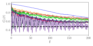
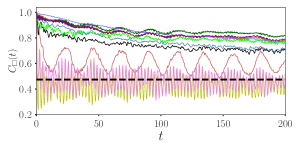
Figure 18: Autocorrelations of individual plaquettes, $C_{\square}(|F\rangle,t)$, for a $10\times 2$ lattice at $\alpha=12$ for a Fock state with an oscillatory average autocorrelation for two independent disorder realizations shown in the top and bottom panels. The different colors represent the local autocorrelation for different elementary plaquettes.

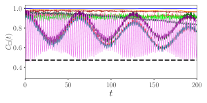
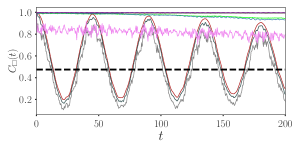
Figure 19: Autocorrelations of individual plaquettes, $C_{\square}(|F\rangle,t)$, for a $10\times 2$ lattice at $\alpha=30$ for a Fock state with an oscillatory average autocorrelation for two independent disorder realizations shown in the top and bottom panels. The different colors represent the local autocorrelation for different elementary plaquettes.

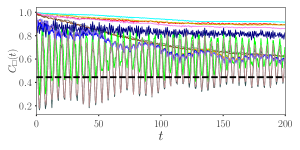
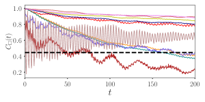
Figure 20: Autocorrelations of individual plaquettes, $C_{\square}(|F\rangle,t)$, for a $6\times 4$ lattice at $\alpha=30$ for a Fock state with an oscillatory average autocorrelation for two independent disorder realizations shown in the top and bottom panels. The different colors represent the local autocorrelation for different elementary plaquettes.

The fraction of Fock states with oscillating average autocorrelations becomes much more significant when the disorder is increased to $\alpha=30$. While we obtained $23$ such Fock states from the randomly chosen $50$ Fock states for the particular disorder realization used in Sec. V.2 for a $10\times 2$ ladder at $\alpha=30$, this number changes to $25$ and $33$ respectively for two other independent disorder realizations shown here. We show the local autocorrelation function, $C_{\square}(|F\rangle,t)$, for one such Fock state for both of the disorder realizations in Fig. 19.

Similarly, while there are $14$ Fock states from the $50$ randomly sampled Fock states with an oscillatory average autocorrelation function for the particular disorder realization shown in Sec. V.2 for a $6\times 4$ ladder at disorder strength $\alpha=30$, this number changes to $6$ and $7$ respectively for two other independent disorder realizations shown here. We show the local autocorrelation function, $C_{\square}(|F\rangle,t)$, for one such Fock state for both of the disorder realizations in Fig. 20.

References

- Deutsch (1991) J. M. Deutsch, “Quantum statistical mechanics in a closed system,” Phys. Rev. A 43, 2046–2049 (1991).
- Srednicki (1994) Mark Srednicki, “Chaos and quantum thermalization,” Phys. Rev. E 50, 888–901 (1994).
- Rigol et al. (2008) Marcos Rigol, Vanja Dunjko, and Maxim Olshanii, “Thermalization and its mechanism for generic isolated quantum systems,” Nature 452, 854–858 (2008).
- D’Alessio et al. (2016) Luca D’Alessio, Yariv Kafri, Anatoli Polkovnikov, and Marcos Rigol, “From quantum chaos and eigenstate thermalization to statistical mechanics and thermodynamics,” Advances in Physics 65, 239–362 (2016), https://doi.org/10.1080/00018732.2016.1198134 .
- Dymarsky et al. (2018) Anatoly Dymarsky, Nima Lashkari, and Hong Liu, “Subsystem eigenstate thermalization hypothesis,” Phys. Rev. E 97, 012140 (2018).
- Sutherland (2004) Bill Sutherland, Beautiful Models (WORLD SCIENTIFIC, 2004) https://www.worldscientific.com/doi/pdf/10.1142/5552 .
- Basko et al. (2006) D.M. Basko, I.L. Aleiner, and B.L. Altshuler, “Metal–insulator transition in a weakly interacting many-electron system with localized single-particle states,” Annals of Physics 321, 1126–1205 (2006).
- Basko et al. (2007) D. M. Basko, I. L. Aleiner, and B. L. Altshuler, “Possible experimental manifestations of the many-body localization,” Phys. Rev. B 76, 052203 (2007).
- Oganesyan and Huse (2007a) Vadim Oganesyan and David A. Huse, “Localization of interacting fermions at high temperature,” Phys. Rev. B 75, 155111 (2007a).
- Nandkishore and Huse (2015) Rahul Nandkishore and David A. Huse, “Many-body localization and thermalization in quantum statistical mechanics,” Annual Review of Condensed Matter Physics 6, 15–38 (2015), https://doi.org/10.1146/annurev-conmatphys-031214-014726 .
- Abanin et al. (2019) Dmitry A. Abanin, Ehud Altman, Immanuel Bloch, and Maksym Serbyn, “Colloquium: Many-body localization, thermalization, and entanglement,” Rev. Mod. Phys. 91, 021001 (2019).
- Anderson (1958) P. W. Anderson, “Absence of diffusion in certain random lattices,” Phys. Rev. 109, 1492–1505 (1958).
- Macé et al. (2019) Nicolas Macé, Fabien Alet, and Nicolas Laflorencie, “Multifractal scalings across the many-body localization transition,” Phys. Rev. Lett. 123, 180601 (2019).
- Serbyn et al. (2013) Maksym Serbyn, Z. Papić, and Dmitry A. Abanin, “Local conservation laws and the structure of the many-body localized states,” Phys. Rev. Lett. 111, 127201 (2013).
- Huse et al. (2014) David A. Huse, Rahul Nandkishore, and Vadim Oganesyan, “Phenomenology of fully many-body-localized systems,” Phys. Rev. B 90, 174202 (2014).
- Pal and Huse (2010) Arijeet Pal and David A. Huse, “Many-body localization phase transition,” Phys. Rev. B 82, 174411 (2010).
- Luitz et al. (2015) David J. Luitz, Nicolas Laflorencie, and Fabien Alet, “Many-body localization edge in the random-field heisenberg chain,” Phys. Rev. B 91, 081103 (2015).
- Bauer and Nayak (2013) Bela Bauer and Chetan Nayak, “Area laws in a many-body localized state and its implications for topological order,” Journal of Statistical Mechanics: Theory and Experiment 2013, P09005 (2013).
- Žnidarič et al. (2008) Marko Žnidarič, Toma ž Prosen, and Peter Prelovšek, “Many-body localization in the heisenberg magnet in a random field,” Phys. Rev. B 77, 064426 (2008).
- Bardarson et al. (2012) Jens H. Bardarson, Frank Pollmann, and Joel E. Moore, “Unbounded growth of entanglement in models of many-body localization,” Phys. Rev. Lett. 109, 017202 (2012).
- Vosk and Altman (2013) Ronen Vosk and Ehud Altman, “Many-body localization in one dimension as a dynamical renormalization group fixed point,” Phys. Rev. Lett. 110, 067204 (2013).
- Vosk et al. (2015) Ronen Vosk, David A. Huse, and Ehud Altman, “Theory of the many-body localization transition in one-dimensional systems,” Phys. Rev. X 5, 031032 (2015).
- Pekker et al. (2014) David Pekker, Gil Refael, Ehud Altman, Eugene Demler, and Vadim Oganesyan, “Hilbert-glass transition: New universality of temperature-tuned many-body dynamical quantum criticality,” Phys. Rev. X 4, 011052 (2014).
- Imbrie (2016a) John Z. Imbrie, “Diagonalization and many-body localization for a disordered quantum spin chain,” Phys. Rev. Lett. 117, 027201 (2016a).
- Imbrie (2016b) John Z. Imbrie, “On many-body localization for quantum spin chains,” Journal of Statistical Physics 163, 998–1048 (2016b).
- De Roeck and Huveneers (2017) Wojciech De Roeck and Fran çois Huveneers, “Stability and instability towards delocalization in many-body localization systems,” Phys. Rev. B 95, 155129 (2017).
- Luitz et al. (2017) David J. Luitz, Fran çois Huveneers, and Wojciech De Roeck, “How a small quantum bath can thermalize long localized chains,” Phys. Rev. Lett. 119, 150602 (2017).
- Devakul and Singh (2015) Trithep Devakul and Rajiv R. P. Singh, “Early breakdown of area-law entanglement at the many-body delocalization transition,” Phys. Rev. Lett. 115, 187201 (2015).
- Šuntajs et al. (2020) Jan Šuntajs, Janez Bonča, Toma ž Prosen, and Lev Vidmar, “Quantum chaos challenges many-body localization,” Phys. Rev. E 102, 062144 (2020).
- Crowley and Chandran (2022) Philip J D Crowley and Anushya Chandran, “A constructive theory of the numerically accessible many-body localized to thermal crossover,” SciPost Phys. 12, 201 (2022).
- Morningstar et al. (2022) Alan Morningstar, Luis Colmenarez, Vedika Khemani, David J. Luitz, and David A. Huse, “Avalanches and many-body resonances in many-body localized systems,” Phys. Rev. B 105, 174205 (2022).
- Bernien et al. (2017) Hannes Bernien, Sylvain Schwartz, Alexander Keesling, Harry Levine, Ahmed Omran, Hannes Pichler, Soonwon Choi, Alexander S. Zibrov, Manuel Endres, Markus Greiner, Vladan Vuletić, and Mikhail D. Lukin, “Probing many-body dynamics on a 51-atom quantum simulator,” Nature 551, 579–584 (2017).
- Sachdev et al. (2002) Subir Sachdev, K. Sengupta, and S. M. Girvin, “Mott insulators in strong electric fields,” Phys. Rev. B 66, 075128 (2002).
- Lesanovsky and Katsura (2012) Igor Lesanovsky and Hosho Katsura, “Interacting fibonacci anyons in a rydberg gas,” Phys. Rev. A 86, 041601 (2012).
- Turner et al. (2018a) C. J. Turner, A. A. Michailidis, D. A. Abanin, M. Serbyn, and Z. Papić, “Weak ergodicity breaking from quantum many-body scars,” Nature Physics 14, 745–749 (2018a).
- Turner et al. (2018b) C. J. Turner, A. A. Michailidis, D. A. Abanin, M. Serbyn, and Z. Papić, “Quantum scarred eigenstates in a rydberg atom chain: Entanglement, breakdown of thermalization, and stability to perturbations,” Phys. Rev. B 98, 155134 (2018b).
- Ljubotina et al. (2023) Marko Ljubotina, Jean-Yves Desaules, Maksym Serbyn, and Zlatko Papić, “Superdiffusive energy transport in kinetically constrained models,” Phys. Rev. X 13, 011033 (2023).
- Chen et al. (2018) Chun Chen, Fiona Burnell, and Anushya Chandran, “How does a locally constrained quantum system localize?” Phys. Rev. Lett. 121, 085701 (2018).
- Royen et al. (2024) Karl Royen, Suman Mondal, Frank Pollmann, and Fabian Heidrich-Meisner, “Enhanced many-body localization in a kinetically constrained model,” Phys. Rev. E 109, 024136 (2024).
- Théveniaut et al. (2020) Hugo Théveniaut, Zhihao Lan, Gabriel Meyer, and Fabien Alet, “Transition to a many-body localized regime in a two-dimensional disordered quantum dimer model,” Phys. Rev. Res. 2, 033154 (2020).
- Pietracaprina and Alet (2021) Francesca Pietracaprina and Fabien Alet, “Probing many-body localization in a disordered quantum dimer model on the honeycomb lattice,” SciPost Physics 10 (2021), 10.21468/scipostphys.10.2.044.
- Sierant et al. (2021) Piotr Sierant, Eduardo Gonzalez Lazo, Marcello Dalmonte, Antonello Scardicchio, and Jakub Zakrzewski, “Constraint-induced delocalization,” Phys. Rev. Lett. 127, 126603 (2021).
- Kogut and Susskind (1975) John Kogut and Leonard Susskind, “Hamiltonian formulation of wilson’s lattice gauge theories,” Phys. Rev. D 11, 395–408 (1975).
- Chandrasekharan and Wiese (1997) Shailesh Chandrasekharan and U-J Wiese, “Quantum link models: A discrete approach to gauge theories,” Nuclear Physics B 492, 455–471 (1997).
- Banerjee and Sen (2021) Debasish Banerjee and Arnab Sen, “Quantum scars from zero modes in an abelian lattice gauge theory on ladders,” Phys. Rev. Lett. 126, 220601 (2021).
- Biswas et al. (2022) Saptarshi Biswas, Debasish Banerjee, and Arnab Sen, “Scars from protected zero modes and beyond in quantum link and quantum dimer models,” SciPost Phys. 12, 148 (2022), arXiv:2202.03451 [cond-mat.str-el] .
- Haque et al. (2022) Masudul Haque, Paul A. McClarty, and Ivan M. Khaymovich, “Entanglement of midspectrum eigenstates of chaotic many-body systems: Reasons for deviation from random ensembles,” Phys. Rev. E 105, 014109 (2022).
- Sau et al. (2024) Indrajit Sau, Paolo Stornati, Debasish Banerjee, and Arnab Sen, “Sublattice scars and beyond in two-dimensional quantum link lattice gauge theories,” Phys. Rev. D 109, 034519 (2024).
- Oganesyan and Huse (2007b) Vadim Oganesyan and David A. Huse, “Localization of interacting fermions at high temperature,” Phys. Rev. B 75, 155111 (2007b).
- Atas et al. (2013) Y. Y. Atas, E. Bogomolny, O. Giraud, and G. Roux, “Distribution of the ratio of consecutive level spacings in random matrix ensembles,” Phys. Rev. Lett. 110, 084101 (2013).
- Bogomolny et al. (2001) E. Bogomolny, U. Gerland, and C. Schmit, “Short-range plasma model for intermediate spectral statistics,” European Physical Journal B 19, 121 – 132 (2001), cited by: 71; All Open Access, Green Open Access.
- Buijsman et al. (2019) Wouter Buijsman, Vadim Cheianov, and Vladimir Gritsev, “Random matrix ensemble for the level statistics of many-body localization,” Phys. Rev. Lett. 122, 180601 (2019).
- Sierant and Zakrzewski (2020) Piotr Sierant and Jakub Zakrzewski, “Model of level statistics for disordered interacting quantum many-body systems,” Phys. Rev. B 101, 104201 (2020).
- Joanes and Gill (1998) D. N. Joanes and C. A. Gill, “Comparing measures of sample skewness and kurtosis,” Journal of the Royal Statistical Society: Series D (The Statistician) 47, 183–189 (1998), https://rss.onlinelibrary.wiley.com/doi/pdf/10.1111/1467-9884.00122 .
- Bar Lev et al. (2015) Yevgeny Bar Lev, Guy Cohen, and David R. Reichman, “Absence of diffusion in an interacting system of spinless fermions on a one-dimensional disordered lattice,” Phys. Rev. Lett. 114, 100601 (2015).
- Gopalakrishnan et al. (2016) Sarang Gopalakrishnan, Kartiek Agarwal, Eugene A. Demler, David A. Huse, and Michael Knap, “Griffiths effects and slow dynamics in nearly many-body localized systems,” Phys. Rev. B 93, 134206 (2016).