On the contributions of extragalactic CO emission lines to ground-based CMB observations

Abstract

We investigate the potential of CO rotational lines at redshifts $z\sim 0-6$ being an appreciable source of extragalactic foreground anisotropies in the cosmic microwave background. Motivated by previous investigations, we specifically focus on the frequency bands and small scales probed by ground-based surveys. Using an empirical parameterization for the relation between the infrared luminosity of galaxies and their CO line luminosity, conditioned on sub-mm observations of CO luminosity functions from $J=1$ to $J=7$ at $\nu=\{100,250\}$ GHz, we explore how uncertainty in the CO luminosity function translates into uncertainty in the signature of CO emission in the CMB. We find that at $\ell=3000$ the amplitude of both CO autocorrelation and cross-correlation with the CIB could be detectable in an ACT-like experiment with 90, 150 and 220 GHz bands, even in the scenarios with the lowest amplitude consistent with sub-mm data. We also investigate, for the first time, the amplitude of the CO$\times$CIB correlation between different frequency bands and find that our model predicts that this signal could be comparable to the amplitude of the cosmic infrared background frequency cross-correlation at certain wavelengths. This implies current observations can potentially be used to constrain the bright end of CO luminosity functions, which are difficult to probe with current sub-mm telescopes due to the small volumes they survey. Our findings corroborate past results and have significant implications in template-based searches for CMB secondaries, such as the kinetic Sunyaev Zel’dovich effect, using the frequency-dependent high-$\ell$ TT power spectrum.

I Introduction

In recent years, high resolution ground-based cosmic microwave background (CMB) surveys, such as the Atacama Cosmology Telescope (ACT [1]) and the South Pole Telescope (SPT [2, 3]), have significantly extended the range of angular multipoles over which the temperature and polarization anisotropies of the CMB have been measured to high precision. Upcoming surveys such as the Simons Observatory [4], as well as the Prime-Cam on the Fred Young Submillimeter Telescope [5] will further extend this range. As the primary CMB fluctuations are exponentially damped at large $\ell$, the dominant sources of power at small scales are additional components which source photons at CMB frequencies – secondary anisotropies of the CMB and extragalactic forerounds. These components are typically assumed to be uncorrelated with the primordial CMB temperature, and are generally written as linear contributions to the CMB temperature decrement at a sky direction $\bm{\theta}$

$$\Delta T^{\rm CMB}(\bm{\theta}) =\Delta T^{\rm Prim}(\bm{\theta})+\Delta T^{\rm tSZ}(\bm{\theta})+\Delta T^{\rm kSZ}(\bm{\theta})$$

$$+\Delta T^{\rm CIB}(\bm{\theta})+\Delta T^{\rm RPS}\cdots,$$ (1)

where the superscripts tSZ and kSZ refer to CMB secondary anisotropies like the thermal and kinetic Sunyaev-Zel’dovich effects, and CIB and RPS denote the cosmic infrared background and contamination from radio point sources which dominate at low frequencies, respectively. The power spectra of each of these components, and their cross correlations, have differing angular dependence and scaling with frequency – templates of these signals have their amplitudes constrained through joint analyses of CMB maps observed at different frequencies [6, 7, 8, 9].

Beyond the additional components of CMB photons discussed above, emission from rotational transitions of CO molecules contained in star-forming galaxies will also source photons at CMB frequencies. Indeed, a photon sourced from the CO$(J\to J-1)$ transition at redshift $z_{\rm em}$ will reach a CMB detector at

$$\nu_{\rm obs}=\frac{J\times 115.271}{1+z_{\rm em}}\,{\rm GHz}\,.$$ (2)

Thus, for frequency bands of ground-based experiments, there is a wide swath of redshifts over which excited transitions fall into observed frequencies, especially at $\nu_{\rm obs}\sim 90,150,220$ GHz. In Fig. 1 we show a visual illustration of Eqn. 2 – how the transitions from $J=1$ to $J=7$ redshift into three of the frequency bands of a typical ground-based CMB experiment. We also show the redshift range over which 16-84% of the intensity of the CIB is emitted, according to the CIB model of the Agora simulation (which we will introduce shortly). It is clear that for higher frequency bands there are many lines sourced at $z\sim 1-3$, the peak epoch of cosmic star-formation-rate density [10], that are redshifted into the frequencies measured by CMB experiments.

The potentially sizable contributions from redshifted CO transitions into CMB bands were originally noted by Ref. [11]. However, the authors correctly noticed that as the spectral energy distribution of a molecular transition is closely approximated by a delta function, this signal was heavily suppressed by the width of the bandpass (by a factor of $\sim 1/\Delta\nu$). The auto-correlation would be further suppressed by $(\Delta\nu)^{-2}$ and it was suggested this signal would be challenging to detect unless radio experiments with very fine frequency resolution were built – now known as line-intensity mapping surveys [12]. However, it was recently pointed out in Ref. [13] (hereinafter M23) that, even though the auto-correlation of this signal is heavily suppressed for CMB surveys, its cross-correlation with the CIB could be significant. The CO$\times$CIB signal in their analysis was potentially comparable to the amplitude of the late-time kSZ effect, which had recently been claimed to be detected at $\sim 3\sigma$-significance in Ref. [9].

Motivated by the fact that a potentially bright extragalactic foreground could be detectable in current ground-based CMB experiments and at the same time may have been biasing template-based and component separation analyses, in this work we produce independent predictions for the frequency-dependent power spectrum of CO fluctuations as well as their cross-correlations with the CIB. This is achieved by leveraging the Agora [14]+SkyLine [15] cosmological N-body simulation suite of the multi-component sky. The fiducial Agora simulation has produced highly accurate CIB maps consistent with Planck, ACT and SPT multi-frequency data which are derived from an empirical star-formation model [10] coupled to a prescription to map star formation to IR luminosity. We use the same large-scale-structure scaffolding and star formation to derive CO luminosities. This allows us to produce full-sky maps of line emission across many transitions of the CO rotational ladder, and study their multi-frequency impact on CMB maps. The use of the full-sky Agora simulation allows us to probe this emission at a larger volume than was able to be done in ite]cite.Maniyar_2023M23.

Additionally, in this work we go beyond standard assumptions for the CO emission ladder and calibrate the individual transitions to observed data at 100 and 250 GHz, near frequencies where ground-based CMB observatories operate. Current measurements of CO luminosity functions, due to their small fields of view, do not sample the entirety of the luminosity function with high precision. We therefore will use the flexibility of our empirical model to attempt to quantify the uncertainty associated with the impact of CO transitions on CMB maps – thus answering the question how much impact on CMB observables is allowed, conditioned on CO luminosity functions consistent with data?.

This paper is structured as follows: in § II we discuss the techniques adopted to simulate IR and CO emission from the underlying large-scale structure of a cosmological halo lightcone, and how we use this catalog to construct maps of CO emission for CO transitions from $(1\to 0)$ to $(7\to 6)$ for three bandpasses representing an ACT-like CMB survey. In § III we present measurements of angular power spectra of the CO maps produced in this work, as well as cross-correlations with CIB maps. We compare these power spectra to the CIB auto-spectrum as well as the imprint of the late-time kSZ effect. We also discuss power spectra across different frequency bins for combinations of CO$\times$CIB. In § IV we present some qualitative discussion on the amplitude of the observed correlations in the previous section. We also compare with predictions for similar observables reported in ite]cite.Maniyar_2023M23. We conclude in § V and discuss future directions that we believe are particularly pertinent in light of the results presented in this publication.

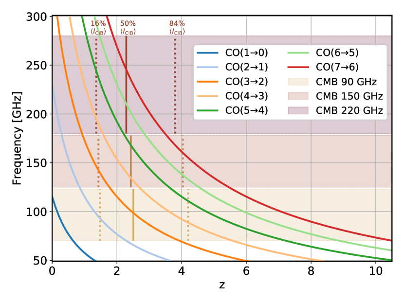
Figure 1: The redshift-observed frequency relation for the CO rotational ladder, compared to frequency bands representative of ground-based CMB surveys. The vertical lines bracket the redshift range from which the average CIB intensity in that band receives the 16%, 50% and 84% of its contribution. Note the significant overlap between several CO lines and the peak of CIB emission.

II Empirical simulations of CMB secondaries and extragalactic foregrounds

Quantifying the amplitude of extragalactic foregrounds and secondary anisotropies is a challenging task. From a halo model modeling perspective, it requires an in-depth understanding of the distribution of halos and their electron pressure profiles (for tSZ), small-scale density profiles (for kSZ), or a detailed understanding of the connection between halo masses and radio / IR luminosity; all within a cosmological context across a wide range of redshift. While halo model approaches have been successful at analytically modeling many of these secondaries (see, e.g., Ref. [16]), building halo models for CO emission is a subject in its infancy, and mainly dedicated to modeling line-intensity mapping observations (see e.g., [17, 18]). Effectively, a halo model for CO emission would have to capture the evolution of the connection between halo mass and the luminosity of a specific CO $J$ transition between $0<z\lesssim 5$, as well as the correlations between different transitions within a specific halo [19].

An alternative approach is to rely on empirical observations of CO luminosity and how it correlates with other astrophysical observables. These empirical data may be used to assign CO luminosities to halos in large N-body simulations, which try to capture the underlying correlations between halo mass and the astrophysical observable which scales with CO luminosity. In the context of CMB secondaries and extragalactic foregrounds these empirically-calibrated simulations have been generated using peak-patch algorithms [20] or by adopting more realistic models which attempt to model star-formation histories for dark matter halos in a fully nonlinear cosmological $N$-body simulation, such as in the SIDES or Agora multi-component sky simulations [21, 22, 14].

In this work, we have elected to use the simulation suite underpinning Agora observables to empirically assign CO luminosities to underlying halos. The shared distribution of halo masses, stellar masses, and star formation rates (SFR) will ensure our CO maps correlate with other extragalactic foregrounds and CMB secondaries in Agora, given our model. The large-scale structure underpinning Agora is the dark matter distribution from the MultiDark Planck 2 cosmological simulation [23], which has a volume of V=1 $[{\rm Gpc}\,h^{-1}]^{3}$ and $N=(3840)^{3}$ particles, resulting in a mass resolution of $M_{p}=1.51\times 10^{9}M_{\odot}h^{-1}$. The Rockstar phase-space halo finder [24] is applied to the resulting particle catalogs, and the empirical UniverseMachine model [10] is then used to assign SFR, stellar masses and star-formation histories to every halo and sub-halo in the catalog. Agora then builds full-sky lightcones from these halo catalogs at different redshifts.

The original Agora publication showed that using stellar masses and SFR derived from UniverseMachine, the resulting lightcones reproduce the correlations of fields which depend on these quantities, such as anisotropies of the CIB, in a way consistent with current data. The fiducial realization of Agora is also tuned to describe summary statistics related to the tSZ effect, the kSZ effect, radio-bright galaxies, cosmic shear, CMB lensing, and more. We refer to Ref. [14] for a more detailed description of how each individual component of Agora is constructed. We note, however, that in this study we use maps of unlensed CIB anisotropies as we anticipate the impact of CMB lensing to be subleading in our observables, and accurately lensing the CO emission we wish to simulate is a computationally challenging procedure [25].

CO transitions	Frequency band
	90 GHz	150 GHz	220 GHz
	Redshift range
CO(1-0)	0-0.5	-	-
CO(2-1)	1.1-2.0	0.3-0.9	0-0.2
CO(3-2)	2.1-3.5	1.0-1.8	0.2-0.8
CO(4-3)	3.1-5.0	1.7-2.7	0.7-1.5
CO(5-4)	4.1-6.5	2.4-3.6	1.1-2.1
CO(6-5)	5.2-8.0	3.0-4.6	1.5-2.7
CO(7-6)	6.2-9.5	3.7-5.5	1.9-3.3

Table 1: Redshift ranges for each CO transition sampled by frequency bands of ground-based observatories, assuming for ACT-like bandpasses. Note that all frequencies receive significant contributions from CO emission at the redshifts over which the contribution of star formation to the CIB peaks, which is between redshifts $1<z<3$.

II.1 Infrared luminosities of halos

Our scheme to sample empirical CO luminosities in dark matter halos will leverage the well-studied connection between CO luminosity and IR luminosity in CO-bright galaxies (see e.g., [26, 27]), and thus we begin by assigning IR luminosities to the halos in our lightcone. It is also important to ensure that our CO luminosities correlate with Agora CIB maps correctly, and thus we will assign IR luminosities to halos in the same way as done in Agora. We briefly recap their approach but refer to Ref. [14] for full details.

A modified Kennicutt relation is used to sample an IR luminosity for every halo according to its SFR and stellar mass ($M_{*}$), following

$$L_{\rm IR}=\frac{\rm SFR}{K_{\rm IR}+K_{\rm UV}{\rm IRX}^{-1}(M_{*})},$$ (3)

where $K_{\rm UV,IR}$ are coefficients with units of $[K_{\rm UV,IR}]=M_{\odot}{\rm yr}^{-1}L_{\odot}^{-1}$ taken from [14], and ${\rm IRX}$ is the IR excess quantifying the ratio between ultraviolet and IR luminosity for a given galaxy. It is parameterized as a power-law in stellar mass [30],

$${\rm IRX}=\left(\frac{M_{*}}{M_{s}}\right)^{\alpha_{\rm IRX}},$$ (4)

with $M_{s}$ and $\alpha_{\rm IRX}$ values taken from Ref. [14]. This results in a close-to-linear relation between IR luminosity and SFR for high SFR, but showing a deficit for low SFR values and overall deviations at high redshifts (see Fig.5 in Ref. [14]). UniverseMachine assigns two types of SFR for a halo, ‘true’ and ‘observed’, and we use ‘observed’ SFRs in Eqn. 3. Since the ‘observed’ SFR and $M_{*}$ drawn by UniverseMachine already include scatter, we do not assign additional scatter and instead evaluate Eqn. 3 directly to assign $L_{\rm IR}$ to a halo. This is consistent with what was implemented in Agora.

The assigned IR luminosity is interpreted as a bolometric value, and in order to compute CIB anisotropies a spectral energy distribution (SED) must be assigned to every halo. Agora adopts a modified black-body SED with a transition frequency into a power law, with slope determined by the dust temperature, $T_{d}$, on a halo-by-halo basis. This dust temperature may be estimated from the SFR and stellar mass of each halo, giving a self-consistent solution for IR luminosity and spectral index arising from only the halo mass, stellar mass and SFR of that halo. This final SED is redshifted according to the halo’s redshift in the underlying lightcone, and the resulting k-corrected flux [31] is integrated against the bandpass of a CMB experiment in order to compute the CMB temperature decrement induced by IR photons coming from an individual galaxy for that experiment.

This is the scheme by which Agora constructs maps of diffuse CIB emission that contaminates CMB maps. Following this scheme to derive other observable quantities ensures that their cross-covariance is taken into account in the simulation suite.

	$\alpha_{\rm IR}$; $\beta_{\rm IR}$; Reference
CO($J\rightarrow J-1$) transitions	Frequency band
	90	150	220
		-	-
1-0	1.27; 1; [27]	-	-
		-	-
	0.91; 2.51	0.98; 1.55;
2-1	0.97; 2.04; [32, 33]	1.03; 1.30; (*)	1.11; 0.6; [27]
	1.19; 0.03	1.15; 0.40
	0.99; 1.65	1.06; 1.02	1.18; -0.56
3-2	1.06; 1.24; [32, 33]	1.06; 1.35; (*)	1.06; 0.85; [32]
	1.31; -0.91	1.3; -0.65	0.94; 2.31
	1.92; -8.04	1.55; -3.72	1.04; 1.31
4-3	3.20; -20.67; [34, 33]	1.83; -6.20; (*)	1.02; 1.69; [32]
	3.60; -23.94	1.98; -7.20	1.02; 2.04
	1.00; 1.08	1.03; 1.58	1.07; 1.29
5-4	1.10; 0.57; [33]	1.07; 1.51; (*)	1.05; 1.79; [32]
	1.28; -1.22	1.29; -0.55	1.30; -0.55
	1.22; -0.75	0.94; 2.56	1.06; 1.54
6-5	1.42; -2.05; (**)	1.02; 1.98; (**)	1.06; 1.74; [32]
	1.62; -3.32	1.11; 1.52	1.16; 0.95
	1.36; -1.65	0.88; 3.23	1.0; 2.2
7-6	1.51; -2.25; (**)	0.98; 2.37; (**)	1.03; 2.06; [32]
	1.67; -3.32	1.08; 1.76	1.07; 1.90

Table 2: Values for the $\alpha_{\rm IR}$ and $\beta_{\rm IR}$ parameters appearing in the $L_{\rm IR}-L^{\prime}_{J}$ relation. We show the values used for each transition and frequency band (corresponding to different redshift ranges, according to Table 1), fit to luminosity functions measured in overlapping redshift ranges (references indicated in the table). Values obtained from interpolating and extrapolating the redshift evolution of the $L^{\prime}$ luminosity functions are denoted by (*) and (**), respectively. Every transition-frequency combination has three values shown, corresponding to (from top to bottom) the ‘shallow’, ‘fiducial’, and ’steep’ luminosity functions discussed in the text.

II.2 CO Luminosity functions

The CO luminosities of every halo, combined with their IR luminosity, are the building blocks of the extragalactic CMB foregrounds we wish to study in this work. Given a realization of the correlated extragalactic sky, we derive CO luminosities across all relevant transitions, on a halo-by-halo basis, using SkyLine  [15], which implements an updated version of the CO painting scheme originally proposed in Ref. [35]. We assume that CO luminosities can be parameterized using power-law relations, starting from IR luminosities that are computed using the scheme described in the previous section. Thus, we relate them to the observed CO luminosity for a given transition $L_{\rm CO}^{J\to J-1}$ with

$$\log L_{\rm IR}=\alpha_{J,\rm IR}\log{L^{\prime}}_{\rm CO}^{J\to J-1}+\beta_{J,\rm IR},$$ (5)

where $\alpha_{J,\rm IR}$ and $\beta_{J,\rm IR}$ are the power-law slope and amplitude for that transition. This relation is not deterministic –values of $L^{\prime}_{\rm CO}$ are sampled from this mean relation and we assume a fixed mean-preserving lognormal scatter of $\sigma_{\rm CO}=0.2$ for all transitions and redshifts. The $L^{\prime}_{\rm CO}$ luminosity, in units of pseudo-luminosity, is related to physical units through

$$L_{\rm CO}=4.9\times 10^{-5}L^{\prime}_{\rm CO}J^{3}\frac{L_{\odot}}{{\rm K\,km\,s^{-1}\,pc^{2}}}\,.$$ (6)

A commonly adopted assumption in the literature is that the ratio between line luminosities at different transitions is constant for all redshifts (see e.g., [36]). CO emission is then modeled assuming $\alpha_{J,\rm IR}=\alpha_{0,\rm IR}$, thus writing that

$$\log{L^{\prime}}_{\rm CO}^{J\to J-1}=\frac{\log L_{\rm IR}-\beta_{\rm IR}}{\alpha_{\rm IR}}+r_{J},$$ (7)

where $r_{J}$ sets the relative line luminosities for each transition across all redshifts. The values of $\alpha,\beta$ are commonly calibrated to low-redshift observations of CO$(1\to 0)$ emitters [27] and then extrapolated to high $z$. On the other hand, studies focused on the COMAP experiment [37] model the CO(1-0) emission at $z\sim 2-3$ using COLDZ+GOODS measurements [34] as anchors.

In this work, however, we will adopt a data-driven approach to connect IR luminosity to CO luminosity for each transition and redshift. Using measurements of luminosity functions of $L^{\prime}_{{\rm CO}(J\rightarrow J-1)}$ from galaxy-survey programs, we find values of $\alpha$ and $\beta$ which connect the $L_{\rm IR}$ distribution in our simulation to these data. In particular, for local galaxies we take results from Ref. [27]. For higher $J$ transitions at higher redshifts, we rely on results from the ASPECS survey using ALMA at 1.2 and 3 mm (250 and 100 GHz, respectively) [32], and NOEMA results [33] also at 1.2 and 3 mm bands.

We use the measured CO luminosity functions at these 100 GHz and 250 GHz to anchor our theoretical predictions of CO contributions for a given CMB bandpass. Certain bandpasses such as 150 GHz do not have accompanying CO luminosity function observations, and so we will interpolate between 100 and 250 GHz observations when inferring $\alpha,\beta$ for that bandpass. We refer the reader to App. A for more information.

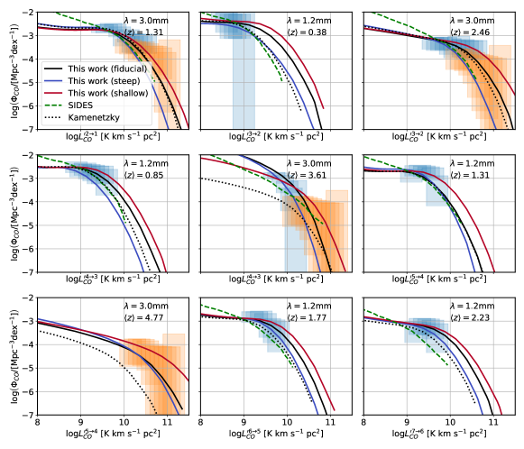
Figure 2: Comparison between the CO luminosity functions measured from sub-mm galaxy susrveys (ASPECs, in blue squares and NOEMA in orange squares), and those obtained from the $\alpha-\beta$ parameterizations presented in this work. The steep, fiducial and shallow luminosity functions we adopt are shown in in blue, black and red, respectively. For each panel, we indicate the observed pivot wavelength of the measurements and the corresponding mean redshift of the sources observed. We also show, for comparison, the CO luminosity functions from SIDES [22] (which underpins the analysis of Ref. [13], in dashed green lines), and the result of extrapolating the local measurements of the $L^{\prime}_{\rm CO}-L_{\rm IR}$ relations from Kamenetzky [27] (in dotted black lines) to the redshifts considered in this work.

We fit $\alpha-\beta$ values to the observed CO luminosity functions using the following procedure:

1. Given the frequency range of a luminosity-function measurement and the corresponding targeted CO transition $J$, we convert this to an observed range in redshift.

2. From the Agora halo lightcones, we select halos within that redshift range and compute their corresponding $L_{\rm IR}$ using the method discussed in Sec. II.1.

3. Given an $\alpha-\beta$ set, we sample a corresponding $L^{\prime J\to J-1}_{CO}$ for every halo in the relevant lightcone using Eqn. 5 and compute the resulting luminosity function of CO.

4. We iteratively sample over $\alpha,\beta$ using a simple least squares optimizer to converge on a reasonable value for the slope and amplitude.

We note that due to the paucity of data for the majority of these transitions, especially at high luminosities for which it is exceedingly difficult that the small field of views surveyed contain such bright objects, there are many combinations of $\alpha_{\rm IR}$ and $\beta_{\rm IR}$ which all give acceptable fits.

In order to quantify the impact of uncertainties in measured CO luminosity functions on the imprint of CO anisotropies in the CMB we generate, for each frequency band and transition, three separate pairs of $\alpha-\beta$ which are consistent with the data. We call these fits “steep”, “fiducial” and “shallow” luminosity functions, as we find that the largest impact in varying $\alpha-\beta$ is at the high-$L_{\rm CO}$ end where the data are unconstrained. We report these values in Table. 2 and show the corresponding luminosity functions compared to data in Fig. 2. Note that Ref. [27] already provide the best-fit $\alpha_{\rm IR}$-$\beta_{\rm IR}$ values for the local luminosity functions; thus, we use these as our fiducial case and do not consider steep or shallow scenarios. Note that, as we will see below, these transitions are very subdominant, so that this choice do not affect our results. We also compare our results, where available, to two previously adopted CO luminosity functions in the literature

• The luminosity function from SIDES [22] simulations, which were used to previously quantify the impact of CO as a contaminant to small-scale CMB anisotropies in ite]cite.Maniyar_2023M23.

• Using the locally measured values of $\alpha_{J}$ and $\beta_{J}$ from low-redshift observations collected in Ref. [27] (henceforth referred to as the ‘Kamenetzky relations’) and extrapolating them to all redshifts in our simulation.

From Fig. 2 we see that the ASPECs data primarily probes the “knee” in the CO luminosity function, leaving significant uncertainty in the high-luminosity regime. Similarly, note that the luminosity functions derived from SIDES are comparable or steeper than our “steep” luminosity functions, where the ‘steepness’ more accurately translates to the approximate exponential cut-off luminosity for a Schechter function fit to the data. Additionally, at lower luminosities than where data are available the SIDES luminosity functions are significantly steeper than what is predicted from our $L_{\rm IR}$-based model. We note that varying the cutoff of our CO luminosity function at its bright end does not strongly alter its slope at the faint end – it is stable for all transitions, including when we use the values from the Kamenetzky relations.

The standard Kamenetzky relations, despite being built on an extrapolation of low-z information assuming that each transition has an identical power-law slope, seem to be in reasonable agreement with measured luminosity functions with the exception of the high-redshift $(5\to 4)$ and $(4\to 3)$ transitions.

II.3 Generating CO maps

Given the above scheme to derive CO luminosities on a halo-by-halo basis from their underlying IR luminosities and a set of $\alpha-\beta$ values, we are now in a position to construct maps of the extragalactic CO that contributes to a given CMB bandpass. The adopted scheme is the same as detailed in Ref. [15], but we summarize it below:

1. Given a CMB frequency band, we identify the corresponding redshift range over which photons originating from a CO transition $J\to J-1$ will be redshifted into that band –shown in Table 1.

2. Shells of width $\Delta\chi=50\,h^{-1}{\rm Mpc}$ that fall within this range are iteratively queried from the lightcone, and a CO luminosity is assigned to each halo using the derived IR luminosity (Eqn. 3) and $\alpha-\beta$ values specified by the corresponding luminosity function, from Table. 2, following Eqns. 5 and 6.

3. Every object in the shell is then given a Dirac delta “SED” $\Phi_{\nu}=L_{\rm CO}\delta^{D}(\nu-\nu_{\rm rest}/(1+z_{\rm em}))$, where $z_{\rm em}$ is the redshift of that halo which relates the rest-frame frequency to the observed through $\nu_{\rm obs}=\nu_{\rm rest}/(1+z_{\rm em})$.

4. This “SED” is integrated against a spectral bandpass $\tau(\nu)$ for an experiment in order to compute the flux at an angular position on the sky sourced by that object into that experiment. Since the SED is a delta-function we find

   $$I_{\nu}^{\rm CO} =\frac{L_{\rm CO}\tau(\nu_{\rm obs})}{4\pi\chi^{2}(z_{\rm em})(1+z_{\rm em})\int d\nu\tau(\nu)},$$ (8)

   $$\approx\frac{L_{\rm CO}}{4\pi\chi^{2}(z_{\rm em})(1+z_{\rm em})\Delta\nu},$$ (9)

   where we have assumed a top-hat pass band in the last equality to explicitly show the $\sim\Delta\nu$ suppression in the CO contribution to the measurements. We use actual ACT-like experimental bandpasses for the main results in this work, but we expect similar conclusions will hold for bandpasses of other ground-based experiments such as SPT or Simons Observatory.

5. The flux is then converted into a spectral radiance by dividing $I_{\nu}/\Omega_{\rm pix}$, where $\Omega_{\rm pix}$ is the solid angle subtended by the desired HEALPix resolution.

6. Given a bandpass we convert this spectral radiance into a CMB temperature decrement $\Delta T_{\nu}^{\rm CO}$, in units of $\mu$K, following Ref. [38].

7. The temperature decrement is summed to the map at the position of that object on the sky, and the previous steps are applied to a new shell, so that

   $$\Delta T_{\nu}^{{\rm CO}(J\to J-1)}(\bm{\theta})=\sum_{n}^{N_{\rm shell}}\sum_{i\in{\rm shell\,n}}\Delta T_{\nu,i}^{{\rm CO}(J\to J-1)}(\bm{\theta}_{i})\,.$$

8. The final result is a HEALPix map which captures all CO$(J\to J-1)$ emission at a given frequency band, across all relevant redshifts.

This procedure produces a map of aggregate CO emission of all line emitters whose lines redshift into an experimental CMB bandpass, $\tau(\nu)$. We note again that, as the singular Dirac delta function SED gets integrated against the bandpass, this signal is suppressed by the width of the band $\Delta\nu$.

In order to suppress bright outliers, every $J$ map also receives a rudimentary flux cut where the brightest $0.1\%$ pixels are masked out. This produces at most a 10% change in the variance of the map, except for the 220 GHz CO$(2\to 1)$ curve which probes the very local Universe, and we found that a small number of bright nearby sources fully dominated the spectrum of the map.

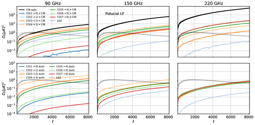
Figure 3: Auto and cross-spectra of individual CO transitions with CIB maps at 90, 150 and 220 GHz, for the “Fiducial” luminosity function shown in Fig. 2, in comparison with CIB auto-spectra and the kSZ signal as predicted from Agora.

III Results: angular power spectra of CO emission

Having produced full-sky maps of CO emission for a transition $J\to J-1$, at a given bandpass $\nu$, we measure their angular auto and cross power-spectra by using the standard anafast routine from the HEALPix library [39]. As the maps produced in this work cover the full sky, we do not require any additional treatment of mode-coupling induced by a survey mask. We additionally apply a $\ell_{\rm min}\sim 100$ for the largest angular scale considered, as the method used to construct lightcones from tiling the original MDPL2 box does not include correlations on scales larger than this. We refer to Ref. [15] for a more detailed discussion.

In summary, we decompose the CO temperature perturbation maps into spherical harmonics

$$\Delta T^{{\rm CO}(J\to J-1)}_{\nu}(\bm{\theta})=\sum_{\ell,m=-\ell}^{\ell}a_{\ell m}^{{\rm CO}(J\to J-1),\,\nu}Y_{\ell m}(\bm{\theta}),$$ (10)

and measure the corresponding auto and cross-spectra with maps of the CIB produced by Agora:

$$C_{\ell}^{\rm CIB,{\rm CO}(J\to J-1)}(\nu)=\frac{1}{2\ell+1}\sum_{m=-\ell}^{\ell}a_{\ell m}^{{\rm CO}(J\to J-1),\,\nu}{a^{*}}_{\ell m}^{\rm CIB,\nu}$$ (11)

$$C_{\ell}^{\rm CO}(\nu)=\frac{1}{2\ell+1}\sum_{m=-\ell}^{\ell}\left|a_{\ell m}^{{\rm CO}(J\to J-1),\,\nu}\right|^{2}.$$ (12)

The resulting auto and cross-spectra for the fiducial luminosity functions adopted in this work are shown in Fig. 3. Specifically, we show the re-scaled power spectra

$$D_{\ell}\equiv\frac{\ell(\ell+1)}{2\pi}C_{\ell},$$

in order to ease comparison with past work.

III.1 The CIB $\times$ CO spectrum

The upper panels of Fig. 3 show the cross-correlation between CO emission and the CIB for three frequency bands corresponding to an ACT-like experiment, of 90, 150 and 220 GHz. Specifically, we show the full contribution to the observed TT power spectrum which is $2\times\langle{\rm CO}\times{\rm CIB}\rangle$, where $\langle{\rm CO}\times{\rm CIB}\rangle$ is the cross-spectrum between the CO map and the CIB map. The gray curve indicates the late-time kSZ signal from the Agora model with $\log(T_{\rm AGN}/{\rm K})=7.8$ and the solid black curves correspond to the CIB autocorrelation for the same bandpass in the fiducial Agora model.

In agreement with results reported in ite]cite.Maniyar_2023M23, we find that for 150 GHz the cross-spectra between aggregate CO emission and the CIB exceed $1[\mu{\rm K}]^{2}$ at $\ell\sim 3000$ –in fact the contribution to the TT power spectrum is closer to 4 $\mu{\rm K}^{2}$. This amplitude is generically higher than that of kSZ secondary anisotropies in Agora.

We now turn to a detailed breakdown of each CO transition’s contribution to a given bandpass for the case of cross-correlations. It is helpful to consider the redshift ranges probed by each transition through each bandpass, remembering that the cosmic SFR density peaks at $z\sim 2$, and that the average CIB intensity peaks at slightly higher redshifts. Figure 1 contains a visual guide for several bandpasses and Table 1 specifies quantitatively the redshift probed by each frequency/transition combination assuming fiducial ACT-like bandpasses.

Again referring to the upper panels of Fig. 3, we see that at 90 GHZ the amplitude of cross-correlation is primarily driven by the CO$(4\to 3)$ transition with a subdominant contribution arising from $(3\to 2)$. Past $\ell\gtrsim 3000$ the spectra for all transitions are similar to flat, Poisson-like shot noise. At this frequency, then, the lines that drive the CIB cross-correlation are located at $z\in[2.1-3.5]$ and $z\in[3.1-5.9]$.

At 150 GHz, the dominant transitions are CO$(4\to 3)$ and CO$(5\to 4)$, which following Table 1 correspond to emission from $z\in[1.7-2.7]$ and $z\in[2.4-3.6]$ – again tracking the peak of cosmic SFR density around $z\sim 2$ and the peak of CIB intensity at the slightly higher $z\sim 2.5$. Turning to the 220 GHz band the dominant transitions are CO$(7\to 6)$ and CO$(6\to 5)$ which are once again tracing the $z\sim 2-3$ region.

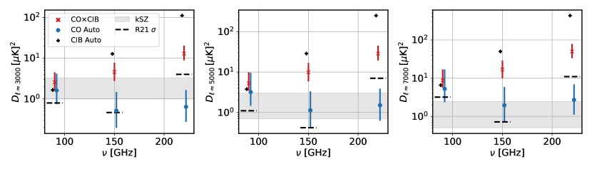
Figure 4: Aggregate contribution for all CO $J$ transitions considered in this work for the auto and cross-spectra, as a function of CMB band considered, for three different angular multipoles. The vertical bars associated with each contribution indicate the lower and upper bounds from assuming every $J$ transition follows its steep or shallow luminosity function, respectively. The gray shaded band corresponds to the kSZ amplitude from the three AGN temperature models discussed in the text. The dashed lines are the 1-$\sigma$ uncertainties from measurements at similar bandpasses for these angular multipoles, from a recent re-analysis of SPT data [9].

Since the CIB is sourced by dusty star-forming galaxies and the CO abundance is similarly a tracer of star-formation and molecular gas, the abundance of which is correlated with that of dust, it is not surprising that the aggregate CO and the CIB show a high level of correlation and that the the prominent drivers of the CO$\times$CIB cross-correlation are consistently the lines which trace the epoch of peak star formation.

Given the uncertainty on the luminosity functions of CO for the range of frequencies and transitions studied in this work (see Fig. 2) we study the impact of varying CO luminosity functions in the CO $\times$ CIB cross-correlation. This result is reported in Fig. 4, where the upper (lower) bars show the result of power spectra measured on maps generated with shallow (steep) luminosity functions. We find that the impact of uncertainty in the CO luminosity function (insofar as accounted for in this study) in this cross-correlation is appreciable but not sufficient to alter prior conclusions about the amplitude of this contribution relative to the kSZ effect. At $\ell=3000$ we find

$$D_{\ell=3000}^{\rm CO\times CIB}\in\begin{cases}[1.7,2.6,4.5]\,\mu{\rm K}^{2},\,\nu=90{\rm GHz},\\ [2.8,4.6,6.3]\,\mu{\rm K}^{2},\,\nu=150{\rm GHz},\\ [8.8,12.9,20.3]\,\mu{\rm K}^{2},\,\nu=220{\rm GHz},\\ \end{cases}$$

in the scenarios where all luminosity functions are simultaneously steep, fiducial or shallow, respectively. This corresponds to a factor of $\sim 2.3-2.6$ variation in the amplitude of this cross-correlation between the two extremes of scenarios entertained here. In the fiducial Agora model, the three kSZ scenarios with $T_{\rm AGN}=\{10^{7.6},10^{7.8},10^{8.0}\}\,{\rm K}$ correspond to power spectra that span the range $D_{\ell=3000}^{\rm KSZ}\in[1,3.5]\mu{\rm K}^{2}$ across all frequencies.

These findings corroborate the results shown in ite]cite.Maniyar_2023M23 and in fact point to the amplitude of the CIB $\times$ CO signal being even larger than they had considered, within our model. Indeed, the SIDES luminosity functions are consistently comparable to the steepest luminosity functions consistent with sub-mm data, as well as having a faint luminosity slope that is steeper than what our model generically predicts. Additionally, we have shown that despite the strong scaling of the CIB amplitude with frequency, at 90 GHz this contaminant still appears significant and comparable to the kSZ effect. Another conclusion one draws from the results in Fig. 4 is that at 90 GHz the CIB$\times$CO cross-correlation is not only of a comparable amplitude to the kSZ effect, but also to the CIB itself. However, it is known that at these frequencies there are larger foregrounds such as the thermal Sunyaev-Zel’dovich effect and shot noise from radio sources which are individually on the order of $\sim 10[\mu{\rm K}]^{2}$ [7]. Thus, we see that the CO$\times$CIB correlation is on the order of 25-45% of these components. Given the uncertainties at $\ell\sim 3000$ for recent ground-based experiments are on the order of $\sigma=0.6\mu{\rm K}^{2}$ this component could be detectable.

III.2 The CO $\times$ CO spectrum

We now turn to the amplitude of the CO auto-spectrum and how it is impacted by uncertainties in CO luminosity functions. The CO auto-spectrum for each line is reported in the lower panels of Fig. 3. We find that the 90 and 150 GHz contributions are dominated by the CO($4\to 3$) transition, and at higher amplitude than previously reported. This large amplitude can be understood as a result of the NOEMA measurements of CO$(4\to 3)$ at 100 GHz, as shown in the central panel of Fig. 2. The NOEMA data prefer a distribution of CO luminosities at significantly higher values than those inferred solely from ASPECs data. Indeed, it has previously been noted that the luminosity function of this specific transition at 100 GHz is not well characterized by a single Schechter function [33]. In contrast, the 220 GHz CO autospectrum receives roughly equal contributions from all transitions considered in this work other than $(2\to 1)$.

While the CO auto-spectrum is suppressed by an additional factor of $1/\Delta\nu$ compared to the cross-correlation previously considered, our analysis highlights that this spectrum has a potentially non-negligible impact as a CMB extragalactic foreground when considered across the entire frequency range. Fig. 4 highlights the aggregate contribution from CO auto as a CMB secondary, again in relation to the CIB, CIB$\times$CO and the kSZ signal. We find, strikingly, that at 90 GHz the CO auto contribution in this model is comparable to if not larger than its cross-correlation with the CIB. However, as mentioned in the previous section, when compared to the dominant foregrounds at 90 GHz the CO auto correlation is still subdominant – with an amplitude on the order of at most 40% that of radio point sources or the tSZ effect. Across the three frequency bands considered we have

$$D_{\ell=3000}^{\rm CO\times CO}\in\begin{cases}[0.8,1.6,4.2]\,\mu{\rm K}^{2},\,\nu=90{\rm GHz}\\ [0.2,0.5,1.2]\,\mu{\rm K}^{2},\,\nu=150{\rm GHz}\\ [0.3,0.6,1.6]\,\mu{\rm K}^{2},\,\nu=220{\rm GHz}\end{cases}$$

This observed – nearly six-fold –variation in the amplitude of CO auto at small scales from uncertainties in the CO luminosity function is significantly larger than what we observed in cross-correlations. This is expected, since the uncertainties are compounded in the case of the auto spectra. The CO auto contribution is suppressed at higher frequencies compared to CO$\times$CIB, but for an experiment with error bars comparable to Ref. [9] they could still be detectable components, especially at $\ell>3000$.

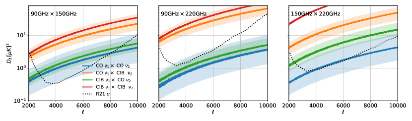
Figure 5: Aggregate CO and CIB auto and cross-correlations between different frequency channels, for transitions up to $J=7$. The dotted black line corresponds to the 1-$\sigma$ of measurements from SPT for similar bandpasses, from Ref. [9].

III.3 Cross-frequency spectra

Having characterized the frequency dependence of the auto and cross-spectra of CO emission in ground-based CMB experiments, we now examine the amplitude of power spectra at differing frequency channels. The cross-frequency spectrum is a complementary probe of CMB extragalactic foregrounds: signals which have a large autocorrelation in one channel can have significantly lowered cross-correlation with another channel, since components such as radio galaxy counts or CIB intensity scale with frequency but in an opposite fashion. In addition, detector-specific noise, which can be prominent in auto-correlations, is not present in cross-correlations.

We measure these cross-frequency spectra with aggregate maps of CO emission and CIB emission for the three bandpasses considered in this work. These are shown in Fig. 5. We observe the CIB cross-frequency spectrum is always dominant relative to any correlation involving just CO lines. However, for $90\times 150$ and $90\times 220$ we see that the low-high CO$\times$CIB cross-correlation (where CO emission comes from the lower frequency map and CIB from the higher frequency map) is in fact comparable to, if not higher, than this component. Specifically, we find for our fiducial model that

$$D_{\ell=3000}\in\begin{cases}[4.5,\,13.2]\,\mu{\rm K}^{2},\,{\rm CIB_{1}\times CIB_{2}},\\ [3.5,\,10.2]\,\mu{\rm K}^{2},\,{\rm CO_{1}\times CIB_{2}},\end{cases}$$

for the $90\times 150$ GHz and $90\times 220$ GHz cross correlations, respectively. In the SPT analysis presented in Ref. [9], the dominant contribution to cross-frequency spectra involving the 90 GHz band was CIB contamination. Given that our fiducial model for CO emission at 90 GHz correlates with the CIB to have an amplitude nearly as high as that of the CIB auto, we conclude that the CO cross-correlation is particularly important in cross-frequency analyses.

The cross-frequency spectrum is particularly interesting if we also consider how uncertainties in CO luminosity functions impact this cross-correlation. The bands in Fig. 5 denote the variation from the “steep” to the “shallow” luminosity functions. We see that the shallow scenario leads to CO₁ $\times$ CIB₂ correlations that are larger in amplitude than the fiducial Agora ${\rm CIB}_{1}\times{\rm CIB}_{2}$ component. An analysis of cross-frequency small-scale CMB secondaries that includes the templates of CO emission should be particularly sensitive to this amplitude. As a heuristic guide for how sensitive current (and future) cross-frequency measurements will be to these components, we also plot the 1-$\sigma$ uncertainties measured from Ref. [9] for similar bandpasses as those considered in this work. We see that the cross-frequency spectra are measured at exquisite precision, and even components such as the CO${}_{1}\times$CO₂ correlation for $90\times 150$ GHz appear to be significant compared to measured uncertainties. Given the relevance of cross-frequency correlations for template-based analyses and component-separation techniques, we conclude that contributions from CO should be considered to avoid suboptimal or even biased results.

The amplitude of this cross-correlation is driven by the $J=4\to 3$ transition and in particular the high-$L$ tail measured by Ref. [33] – around 45% of the total ${\rm CO}_{1}\times{\rm CIB}_{2}$ amplitude for $\nu_{1}=90,\,\nu_{2}=150$ GHz comes from this particular transition. However, even the $J=3\to 2$ and $J=5\to 4$ transitions in the fiducial scenario possess amplitudes of $D_{\ell=3000}\sim\{0.9,0.5\}\mu{\rm K}^{2}$ respectively which are of similar amplitude to the SPT 1-$\sigma$ bandpass for this frequency combination.

IV Discussion

IV.1 Analytic scalings for the shot-noise term

We have generated maps of extragalactic CO emission at various redshifts conditioned on observations of CO luminosity functions from small-field-of-view sub-mm surveys at similar frequencies. The measurements of the luminosity functions employed allow for freedom in the predicted high-$L^{\prime}$ tail, which in turn results in a significant uncertainty in the amplitude of CO auto correlations and its cross correlations with other CMB secondary anisotropies and extragalactic foregrounds. Here we discuss a simple analytic argument which connects the amplitude of the spectra to the luminosity function, focusing in particular on the uncertainties at the bright end of the luminosity functions.

In Appendix C we show that for the majority of cross-spectra measured in this work, the contribution at $\ell\sim 3000$ (the best-measured multipole) becomes driven by the shot-noise contribution, rather than the clustering component. For tracer auto-spectra, it is well-known that the shot-noise contribution essentially corresponds to the second moment of the flux distribution [7]

$$C_{\ell}^{\rm shot}=\int dS\frac{dN}{dS}S^{2},$$ (13)

where $N$ is the absolute number of emitters in the volume probed by that frequency band. For the CO contribution of a given $J$ transition, we can condition the flux distribution on redshift through the bandpass. Assuming for this argument a top-hat bandpass for simplicity, we are left with

$$C_{\ell}^{\rm shot} =\int dS\frac{dN}{dS}S^{2}$$ (14)

$$=\int_{z_{\rm min}}^{z_{\rm max}}dz\,dS\frac{d^{2}N}{dzdS}S^{2}$$ (15)

where $[z_{\rm min},z_{\rm max}]=[\nu_{\rm rest}/\nu_{\rm max}-1,\nu_{\rm rest}/\nu_{\rm min}-1]$. Converting fluxes to luminosities (using Eqn. 9) we get

$$C_{\ell}^{\rm shot} =\int_{z_{\rm min}}^{z_{\rm max}}dz\,dS\frac{d^{2}N}{dzdS}S^{2}$$

$$=\int_{z_{\rm min}}^{z_{\rm max}}dz\,dL\frac{d^{2}N}{dzdL}\frac{1}{\Delta\nu^{2}}\left(\frac{L}{4\pi(1+z)\chi^{2}(z)}\right)^{2}$$

$$=\frac{c}{4\pi(\Delta\nu)^{2}}\int_{z_{\rm min}}^{z_{\rm max}}\frac{dz}{H(z)}\,dL\,\frac{d^{2}n}{dzdL}\frac{L^{2}}{\chi^{2}(z)(1+z)^{2}}\,,$$ (16)

where $n$ is now, instead, the number density of emitters. Eqn. 16 then makes it clear how a shallower luminosity function at a given redshift will fundamentally lead to a higher shot noise. Eqn. 16 also shows that what is fundamentally being probed is the joint redshift–luminosity distribution function of line emitters in the Universe.

If one wishes to extend this discussion to cross-line emission or CO$\times$CIB correlations, then one must realize that the underlying driver of CO luminosity is the IR luminosity (Eqn. 7), or SFR/$M_{*}$ (Eqn. 3) and the shot-noise is then driven by expectations of the sort

$$C_{\ell}^{\rm shot}\sim\langle L_{\rm CO}(L_{\rm IR})\times L_{\rm IR}\rangle\,\,{\rm or}\,\,\langle L_{\rm CO}({\rm SFR})\times L_{\rm IR}({\rm SFR})\rangle.$$

These correlations are equivalent to Eqn. 16, but changing the $L^{2}(d^{2}n/dzdL)$ term by a term like $\propto L_{\rm CO}L_{\rm IR}(d^{3}n/dzdL_{\rm CO}dL_{\rm IR})$, with the corresponding correlation between the CO and IR luminosities as discussed in Appendix B.

For models such as Eqn. 7 where we have $L_{\rm CO}\propto L_{\rm IR}^{1/\alpha_{J,{\rm IR}}}$ then we see that the CO$\times$CIB does not probe the second moment of the $L_{\rm IR}$ distribution, but really in some sense the expectation $\langle L_{\rm IR}^{1+1/\alpha}\rangle$ – we refer the reader to Appendix B for a more detailed discussion of the formulae of cross shot noise and under what conditions the above expectation is in fact being probed.

Let us consider now a toy model where all emission comes from a delta-function distribution of redshift to get additional insight on the relation between the luminosity function and the Poisson shot noise. In this toy model the geometric factors are fixed and do not contribute to changes in the variance of fluxes, and changes in the luminosity functions are the only sources of changes to the shot noise. We note that for many of the panels in Fig. 2, a Schechter function of the form

$$dn=n_{*}\left(\frac{L}{L_{*}}\right)^{\alpha}e^{-L/L_{*}}d\left(\frac{L}{L_{*}}\right),$$ (17)

can fit the model curves, despite not being an input into either SIDES or our fiducial model for CO luminosities. For concreteness we take the luminosity functions for CO$(2\to 1)$ at 90 GHz and fit $n_{*},\alpha,L_{*}$ to the reported curves. We find that $\alpha=-0.6$, $L_{*}=1.2\times 10^{10}L_{\odot}$ and $\alpha=-0.2$, $L_{*}=1.5\times 10^{10}L_{\odot}$ are a reasonable fit to the luminosity functions of SIDES and the fiducial SkyLine scenario, respectively. The inferred values of $n_{*}$ are very similar for both cases. This is is in agreement with the requirement of recovering the total number density of CO emitters in the redshift shell. Assuming there is a minimal cutoff CO luminosity $L_{0}$ below which halos do not emit CO, as well as extending the upper limit of the integral to infinity, the variance of CO luminosity is given by (up to a volumetric factor)

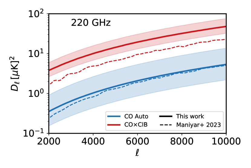
Figure 6: Templates for aggregate CO contamination at 220 GHz compared to the predictions from the SIDES simulation as shown in M23. The CO auto shot-noise is consistent between both simulations, however we see that our simulations predict a significantly higher cross-correlation than previous work. In this figure we explicitly show the correlation $\langle{\rm CO}\times{\rm CIB}\rangle$ instead of its aggregate contribution to CMB spectra as shown in prior figures. The shaded bands around our fiducial predictions encompass the steep and shallow luminosity functions considered in this work.

$$\langle L^{2}\rangle \propto\int\frac{dn}{dL}L^{2}dL$$ (18)

$$\propto{L_{*}}^{2}\int_{L_{0}}^{\infty}\left(\frac{L}{L_{*}}\right)^{2+\alpha}e^{-L/L_{*}}\,d(L/L_{*})$$ (19)

$$\propto n_{*}{L_{*}}^{2}\Gamma(3+\alpha,\frac{L_{0}}{L_{*}}),$$ (20)

where $\Gamma(3+\alpha,\frac{L_{0}}{L_{*}})$ is the upper incomplete Gamma function [42]. The incomplete Gamma function is a strictly monotonically decreasing function in its second argument, peaking at $L_{0}/L_{*}=0$, while monotonically increasing in its first argument, $3+\alpha$. Therefore, we find that both a higher $L_{*}$ at fixed $\alpha$ and a higher $\alpha$ at fixed $L_{*}$ lead to a higher $\langle L^{2}\rangle$. Since for SIDES $\alpha=-0.6$, which is lower than the value for SkyLine, and their luminosity functions frequently cut off at $L_{*}$ consistent with our ‘steep’ luminosity functions – corresponding to low values of $L_{*}$ –, we should generically expect that our model will produce CO maps with higher shot noise components than those of SIDES . Assuming $\log L_{0}=8$, we find the second argument of the upper incomplete Gamma function is close to saturated and we may neglect its dependence. Then, for the specific parameters in this scenario we find that the ratio of moments is

$$\frac{\langle L^{2}\rangle_{\rm\tiny SkyLine}}{\langle L^{2}\rangle_{\rm\tiny SIDES}}\sim\left(\frac{1.5}{1.2}\right)^{2}\frac{\Gamma(2.8)}{\Gamma(2.4)}\sim 2.1,$$

which are of similar order to the differences in CO shot noise we will find in the next section.

Since the joint IR-CO shot noise will be driven by similar underlying mechanisms we expect that these arguments should similarly hold. However, it would be important to examine the underlying distribution of IR fluxes / luminosities between the two simulations and see if the same qualitative differences are observed compared to the CO luminosity functions we have examined in this work. Another challenge in the case of IR luminosity is that the broad SEDs require some additional care compared to our treatment of CO line emission which can be readily treated as a Delta function – again we refer to Appendix B for more discussion on this note.

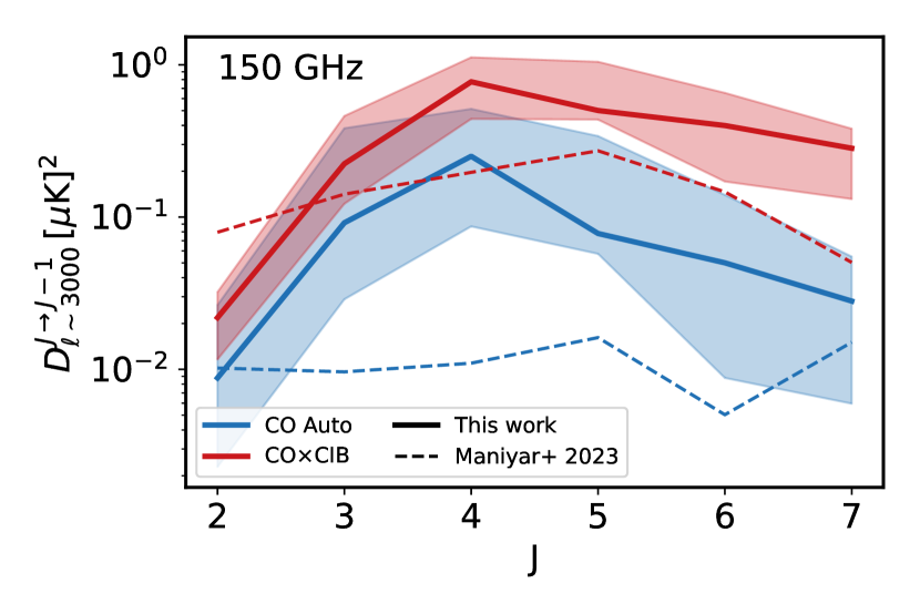
Figure 7: The amplitude of CO power spectra at $\ell=3000$ and 150 GHz for each transition from CO$(2-1)$ to CO$(7-6)$ compared to the SIDES predictions reported in M23.

IV.2 Comparison with previous work

There has been previous work to characterize the amplitude of extragalactic CO signal and its cross-correlation with other sources of anisotropies such as the CIB and the tSZ, mainly the work presented in ite]cite.Maniyar_2023M23. In this section we proceed to compare when possible the predictions generated from our model with theirs. Mainly, we compare to the published aggregate CO autospectra and CO$\times$CIB spectra for a 220 GHz bandpass, as well as a line-by-line comparison for the auto and cross contributions at 150 GHz. We caution that these comparisons will not be one-to-one for many reasons, including that we have used the full ACT bandpass in this work whereas the study presented in ite]cite.Maniyar_2023M23 uses top-hat bandpasses of width $\Delta\nu=50$GHz, as well as adopting a different treatment to mask bright sources. The predictions shown in ite]cite.Maniyar_2023M23 are predicated on the CONCERTO-SIDES simulation [22], which were developed with the intention of mocking up [CII] intensity mapping surveys at high redshift for which extragalactic CO is a significant contaminant. The underlying mechanism for modeling the luminosity of CO lines is also entirely different from the empirical approach we have adopted. However, it is still interesting to see how these different approaches to simulating the same signal compare to each other.

In Fig. 6 we show the aggregate CO auto and CO$\times$CIB spectra for the 220 GHz band as generated in this work and reported in ite]cite.Maniyar_2023M23. We see that at this frequency, our fiducial scenario generates a CO auto-spectrum that is consistent with their work. However, we also see that our fiducial scenario generates a prediction for the CO$\times$CIB spectrum which has similar angular dependence (consistent with being shot noise) but has a higher amplitude than the prediction from SIDES . The steep scenario is $\sim$ 50% higher than what they report, and the fiducial scenario is close to twice higher. As discussed previously, and seen in Fig. 3, our signal is driven primarily by the $(7\to 6)$ and $(6\to 5)$ transitions as their contribution to the band is entirely contained within the peak redshift of the CIB intensity. However, we do not have similar line-by-line comparions of the SIDES 220 GHz spectrum to assess which are the dominant contributions.

For 150 GHz, however, ite]cite.Maniyar_2023M23 breaks down their CO auto and cross spectra by transition. Therefore, in Fig. 7 we have elected to compare our predictions at the fixed angular scale of $\ell=3000$ in order to compare how each $J$ line contributes to the observed band in each model. We find that at 150 GHz our model is consistently higher in amplitude for both auto and cross-spectra. For cross-spectra there is some broad agreement, and the $J$ dependence has a similar ‘rising and falling’ shape across both models, with a peak at $J=4$ for our model and $J=5$ for SIDES . The auto-spectra are different in amplitude and $J$-dependence. Our model predicts, again, a peak at $J=4$ with $D_{\ell\sim 3000}^{4\to 3}\sim 2\times 10^{-1}[\mu{\rm K}]^{2}$ and a faster fall-off than the CIB cross-correlation. For SIDES , however, the J dependence is nearly flat and $D_{\ell\sim 3000}\sim 10^{-2}[\mu{\rm K}]^{2}$ for nearly all of their spectra. It would be especially interesting to compare the predictions of CO luminosity functions between these two models at 150 GHz, as there are no surveys trying to measure this observable at these wavelengths. However, we leave this detailed comparison between these two models for future work.

The analytic scaling arguments presented in the previous sub-section can qualitatively explain why the fiducial model in this work generically predicts a higher amplitude of CO auto and cross-spectra with the CIB compared to previous attempts to characterize this signal. In this subsequent subsection we have further investigated and quantified differences between the two models, focusing on 150 and 220 GHz where the CONCERTO-SIDES suite has been used to generate predictions for extragalactic CO contamination. For 150 GHz we find a strong enhancement of the CO auto relative to their results, and somewhat comparable CO$\times$CIB spectra. For 220 GHz the CO auto are in good agreement and CO$\times$CIB are discrepant by a factor of $\sim 1.5-2$.

IV.3 Comments on the predicted luminosity functions

As discussed in Sec. II, we use $\alpha_{\rm IR}$-$\beta_{\rm IR}$ values obtained from fits to measured luminosity functions, with the corresponding uncertainties and steep/fiducial/shallow scenarios. However, as shown in Fig. 2, in all cases but the $(4\to 3)$ transition at $\langle z\rangle=3.61$, the luminosity functions produced for all three scenarios feature a very similar faint end. This might be due to limitations on the parameterization based on Eqn. (5) but also due to the limited resolution of the MDPL2 simulations employed as underlying halo distribution. In turn, SIDES used the Uchuu simulations, which has a higher resolution, which may explain their higher faint end of the luminosity function. In any case, estimations of the shot-noise contribution – which dominates the signal of interest – using the Schechter fit discussed above show that this difference amounts to $<1\%$ difference in the predicted power spectra. Nonetheless, this feature warrants further investigation, given its relevance for line-intensity mapping dedicated surveys, which target the faint end of the luminosity functions.

We also note, in passing, that another fundamental driver in discrepancies could be the IR luminosity modeling of both approaches. Indeed, the SIDES predictions tend to somewhat under-predict the amplitude of the CIB power spectra compared to Planck and Herschel/SPIRE data (see Fig. 3 of Ref. [43]) and we would expect that under-estimating IR anisotropies could lead to compounding differences between our two predictions for CO emission. Their usage of a pure Kennicutt relation to assign IR luminosities from star formation rates would also lead to significant changes in the faint-end of the $L_{\rm IR}$ distribution, which may result in the higher abundance of faint CO emitters predicted with SIDES with respect to our results. It would be of great interest to further explore differences in the $L_{\rm IR}$ distributions between different simulations of extragalactic foregrounds, since these are the initial building blocks of CIB and IR line-emission models.

V Conclusions

In this work we have used the semi-empirical intensity mapping modeling code, SkyLine, conditioned on observations of CO luminosity functions, from $J=1$ to $J=7$, covering $z\sim 0$ to $z\sim 9$, to generate maps of extragalactic CO emission through bandpasses of ground-based low frequency CMB surveys, specifically for ACT-like bandpasses at 90, 150, and 220 GHz. We generated three sets of maps, corresponding to CO luminosity functions featuring bright-end cutoffs at different luminosities, as the available data do not always probe this regime with enough precision. Our fiducial model often generates a CO luminosity function very similar to assuming locally measured scaling relations from Ref. [27], except for the high-redshift $(4\to 3)$ and $(5\to 4)$ transitions measured at 100 GHz.

We have used these maps to measure each line’s power spectra and cross-spectra with accurate simulated maps of the CIB from the Agora simulations, whose large-scale structure, star formation, and derived IR luminosities are self-consistent with our simulation. We have found, consistent with prior expectations, that the aggregate CO$\times$CIB spectrum is always larger in amplitude than the CO auto-spectrum, with an angular dependence for both types of spectra that is wholly consistent with the shot-noise component at $\ell\gtrsim 2000$, for all frequencies considered. We additionally found that the aggregate signal, at $\ell\sim 3000$, is comparable to or brighter than the late-time kSZ power spectrum from the the Agora simulation.

For the first time we also investigated the cross-frequency spectrum of extragalactic CO, finding that cross-correlations of CO emission at 90 GHz with the CIB at 150 GHz were comparable to the CIB cross-frequency spectrum. Given that this cross-frequency spectrum is exquisitely well measured, and that the dominant extragalactic foreground considered thus far has been this CIB cross-spectrum, these results indicate a promising avenue through which this extragalactic CO foreground can be constrained. This ${\rm CO}_{1}\times{\rm CIB}_{2}$ spectrum may be the second-largest foreground behind ${\rm CIB}_{1}\times{\rm CIB}_{2}$ at 90 GHz $\times$ 220 GHz.

A brief investigation was also conducted comparing the predictions of our empirical model to the CONCERTO-SIDES suite of simulations [22], which were used in ite]cite.Maniyar_2023M23 to similarly quantify this extragalactic CO foreground. We found some instances of agreement at 220 GHz but disagreement in our results, especially the amplitude of CO auto spectra, at 150 GHz. Given the potential impact of including templates of CO emission motivated by our simulations in analyses of CMB survey data a more detailed comparison between the two models is of pressing importance in follow-up studies.

The measured spectra can be readily folded into analyses of ground-based CMB data, and the tools we have developed can be extended to any bandpass for any existing CMB survey. We believe it will be interesting to see what the impact of including our templates is, for example, in inference on the amplitude of the kSZ effect in the CMB temperature power spectrum, or even in potential inference on the shot-noise component of the CIB which we expect is highly correlated with the CO signal. Furthermore, neglecting the extragalactic CO foreground could impact component-separation analyses of the CMB. [CII] emission ($\nu_{\rm rest}=1.9$ THz) might also be expected to be a contaminant for the Planck HFI bands.

The maps in this work can also be used to readily investigate other potential sources of contamination by CO in CMB cross-correlations. For example, an analysis of galaxies from the unWISE galaxy catalog (which are IR luminous, and therefore should also have CO emission) revealed a detection of a higher than expected amplitude for the kSZ effect [44]. It is not inconceivable that correlations between unWISE galaxies and unresolved CO emission in a CMB map could be detected at high significance. Indeed, a detection of diffuse [CII] emission at $z\sim 2.6$ was reported using a cross correlation of Planck HFI and BOSS quasars [45]. Other potentially interesting avenues of our work could be related to using higher-order statistics of the CMB temperature map or in cross correlation with tracers of the large-scale structure, such as bispectra, to tease out components which allow us to better constrain the properties of CO emission through a given bandpass and ideally break degeneracies between the emission from different transitions. If successful, these investigations would be complementary to line-intensity mapping experiments, which are expected to probe the faint-end of the line-luminosity functions.

Another possible scenario is that the low-frequency Poisson components of current CIB models compensate for the presence of CO emission. For example, the Agora CIB model has a Poisson component that fully accounts for the small-scale cross-frequency power spectrum (such as 90 $\times$ 150 GHz). The addition of a CO $\times$ CIB component at the fiducial values here could lead to a potential over-estimate of small-scale power for this frequency correlation. The correct procedure, then, would be to jointly account for the contributions of CO and CIB when fitting to small-scale spectra across a wide range of frequency bands. Since CO luminosity is sourced by IR luminosity, we expect these amplitudes to be correlated. Lowering the amplitude of the CIB component (since we have properly accounted for its joint presence with CO) would also potentially lead to lower amplitude CO components. We defer these sorts of investigations to future work.

We conclude with a final remark that it would be highly desirable to develop an accurate and simply parameterized model for the CO emission that could be easily folded into small-scale CMB likelihood analyses. Our fiducial simulations show that there is significant uncertainty in the amplitude of this signal, and a compact parameterization that properly captures both auto and cross-clustering across frequencies, would be highly desirable. For example, a parameterized conditional distribution of IR and CO luminosity that can be used as input into Eqn. 16. This is not expected to be trivial – each bandpass probes each transition at significantly different cosmic epochs, and even the CIB probes different epochs at different bandpasses. It is not expected that a simple frequency-scaling exists that can capture such large time evolution, but we leave these investigations and this construction to future work. In light of the significant improvements expected to come in the next generation of ground-based observations, such as those from Simons Observatory, we believe developing a model for such a potentially prominent astrophysical signal should be significantly timely.

Appendix A Choice of $\alpha_{\rm IR}$-$\beta_{\rm IR}$ values for transitions and redshifts not covered by observations

As described in Sec. II.2, we follow a data-driven approach to model the CO emission at each transition and redshift we need. However, not all cases of interest are probed by observations. This is the case for the $(6\to 5)$ and $(7\to 6)$ transitions at 90 GHz, and all transitions at 150 GHz. In order to fill this gap, we use the existing measurements for other transitions and frequencies to inform the choice of suitable $\alpha_{\rm IR}$-$\beta_{\rm IR}$ sets, following two different approaches.

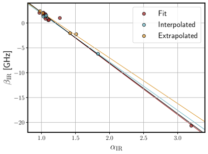
Figure 8: Correlation between the $\alpha_{\rm IR}$ and $\beta_{\rm IR}$ parameter values obtained from the fit to observations (red), interpolated (blue) and extrapolated (orange) luminosity functions from other redshifts and transitions. We also show linear regressions using the same color code (the black line shows the fit to all values); all fits have $R^{2}>0.989$. As it can be appreciated, the values obtained in the interpolation and extrapolations agree well with those from observations.

For those transitions at 150 GHz for which there are available measurements at 90 and 220 GHz (i.e., from $J=2$ up to $J=5$), we choose $\alpha_{\rm IR}$-$\beta_{\rm IR}$ values so that the resulting luminosity function at 150 GHz – obtained following the same procedure as described in § II.2 – lies between the luminosity functions for the same transition at 90 GHz and 220 GHz. This should be an acceptable estimate, since for $J<4$ the corresponding redshifts at 150 GHz are below the redshifts at which the cosmic SFR density peaks, and therefore we can expect a monotonic evolution for the CO luminosity. Transitions with $J=4$ and $J=5$ are more subtle, since the redshifts of interest are around the peak cosmic SFR density. In addition, the luminosity functions of these transitions at 90 GHz are peculiar when compared with the rest – they are the only ones for which the Kamenetzky [27] fit values are ruled out by the data and they may require two Schechter functions to fit observations. We refer to this set of choices as interpolated.

In turn, there are no available measurements for the $(6\to 5)$ and $(7\to 6)$ transitions at 90 GHz either, such that we lack any anchor at higher redshifts for the luminosity function. Here, we use trends of the ratios between the luminosity functions at 220 GHz and the fact that the redshift ranges probed at 150 GHz and 90 GHz are above those for which the cosmic SFR density peaks to choose the $\alpha_{\rm IR}$-$\beta_{\rm IR}$ values. Thus, we refer to these values as extrapolated. Note that, given how high the redshift this emission comes from is, we expect their contribution to be negligible in any case, as we find in Fig. 3.

We report the whole set of $\alpha_{\rm IR}$-$\beta_{\rm IR}$ values in Table 2, and show a visual representation of them in Fig. 8. We can see how the values are highly correlated, and that the three kind of sets – those that we have observations to fit to, interpolated, and extrapolated – show a very similar correlation. Furthermore, all interpolated and extrapolated cases are fairly consistent with the fits reported in Ref. [27] using local measurements.

We therefore acknowledge that our predictions at 150 GHz rely on the interpolated and extrapolated luminosity functions. However, we believe that until there are observations at 150 GHz to calibrate any model to, even an ab initio model that self-consistently predicts all transitions at all redshifts may be inaccurate. We attempt to capture at least part of this uncertainty with the differences between the shallow and steep scenarios.

Appendix B The structure of cross shot-noise between $L_{\rm IR}$ and $L_{\rm CO}$

If we are considering, simultaneously, the cross shot-noise from IR flux (‘1’) and CO flux (‘2’) coming from the same emitter, then expression is given by

$$C_{\ell}^{\rm\times shot} =\int dS_{1}dS_{2}\frac{dN}{dS_{1}dS_{2}}S_{1}S_{2}$$ (21)

$$=\int dzdS_{1}dS_{2}\frac{dN}{dS_{1}dS_{2}dz}S_{1}S_{2}.$$ (22)

Here, the redshift integral in principle runs from $0\leq z<\infty$, as an IR SED can be arbitrarily redshifted into the bandpass of an experiment. However, since we are also considering line emission through this bandpass the integral bounds are the same as in the CO auto shot-noise case. The IR flux of a source through a CMB experiment is written as

$$S_{\rm IR}(z)=\frac{L_{\rm IR}}{4\pi\chi^{2}(z)(1+z)}\frac{\int d\nu\tau(\nu)\Phi_{\rm IR}(\nu(1+z))}{\int d\nu\tau(\nu)},$$ (23)

where $\tau(\nu)$ is the experimental bandpass and $\Phi_{\rm IR}(\nu)$ the modified black-body SED used to describe IR luminosity. The frequency-dependent contribution of this flux can be re-written as the average of the redshifted SED, $\bar{\Phi}_{\rm IR}(z)\equiv\int d\nu\tau(\nu)\Phi_{\rm IR}(\nu(1+z))/\int d\nu\tau(\nu)$. Following arguments analogous to those used to derive the auto shot-noise in § IV, we arrive at the form for the cross-shot-noise

$$C_{\ell}^{\times\rm shot}=\frac{c}{4\pi\Delta\nu}\int_{z_{\rm min}}^{z_{\rm max}}\frac{dz}{H(z)}dL_{1}dL_{2}\frac{d^{3}n}{dzdL_{1}dL_{2}}\frac{\bar{\Phi}_{\rm IR}(z)L_{1}L_{2}}{\chi^{2}(z)(1+z)^{2}}.$$ (24)

The conditional luminosity function, that is, the number density of sources that are simultaneously at redshift $z$ with IR luminosity $L_{1}$ and CO luminosity $L_{2}$, can be rewritten as a probability distribution function as $d^{3}n/dzdL_{1}dL_{2}=\bar{n}(z)P(L_{1},L_{2}|z)\,$. Adopting Eqn. 5 we may directly write $\bar{L}_{2}(L_{1})=10^{-\beta_{\rm IR}/\alpha_{\rm IR}}L_{1}^{1/\alpha_{\rm IR}}$, and we may additionally leverage the fact that we assumed a log-Normal distribution between $L_{2}$ and $L_{1}$ to write

$$P(L_{1},L_{2}|z) =P(L_{2}|L_{1},z)P(L_{1}|z)$$ (25)

$$=P(L_{1}|z)\frac{1}{L_{2}\sqrt{2\pi\sigma^{2}}}\exp\left(-\frac{(\ln L_{2}-\ln L_{1}/\alpha_{\rm IR}+\ln(10)\beta_{\rm IR}/\alpha_{\rm IR})^{2}}{2\sigma^{2}}\right),$$ (26)

where $\sigma^{2}$ is the mean-preserving lognormal scatter, rescaled to the natural logarithm base. A prediction for the number density of CO emitting galaxies $\bar{n}(z)$, and a specific distribution for IR luminosities at a redshift $z$, $P(L_{1}|z)$, are the remaining ingredients required to specify an analytic model of the cross shot-noise.

Assuming the upper integration limit in $L_{2}$ is infinite we may integrate over $L_{2}$ and find

$$C_{\ell}^{\times\rm shot}=\frac{10^{\sigma^{2}/2-\ln(10)\beta_{\rm IR}/\alpha_{\rm IR}}\,c}{4\pi\Delta\nu}\int_{z_{\rm min}}^{z_{\rm max}}\frac{dz\,\bar{\Phi}_{\rm IR}(z)}{H(z)\chi^{2}(z)(1+z)^{2}}dL_{\rm IR}\frac{d^{2}n}{dL_{\rm IR}dz}L_{\rm IR}^{1+1/\alpha_{\rm IR}}.$$ (27)

Given all of these ingredients, we see the cross-shot noise depends on the luminosity function of IR luminosities, and we see that a redshift-weighted moment of the form $\langle L_{\rm IR}^{1+1/\alpha}\rangle$ drives the observed cross-shot noise, as discussed in the main text.

Perhaps interestingly, despite having the highest cross shot-noise we see that $\alpha_{\rm IR}$ for the CO$(4\to 3)$ transition at low frequencies has the highest value – implying a potentially lower shot noise than if $\alpha_{\rm IR}$ were low. However, since $\alpha_{\rm IR}$ and $\beta_{\rm IR}$ are highly anticorrelated (see Fig. 8) a large value of $\alpha_{\rm IR}$ begets a highly negative value of $\beta_{\rm IR}$. The amplitude of the shot noise depends on a pre-factor of $10^{-\beta_{\rm IR}/\alpha_{\rm IR}}$, relating $L_{\rm CO}$ to $L_{\rm IR}$. This will compensate for the moment probed not being as large.

Appendix C Assessing scales at which CO emission is Poisson dominated

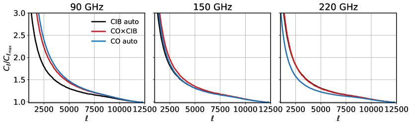
Figure 9: Ratio of $C_{\ell}$ to the largest angular multipole measured for each frequency band / tracer combination. Under the assumption $C_{\ell_{\rm max}}$ is dominated by the Poisson shot noise component, this ratio measures the relative contributions of clustering to Poisson. We see that all tracers begin to be dominated by the Poisson component (i.e., $C_{\ell}/C_{\ell_{\rm max}}<2$) at $\ell>3000$.

The analytic scaling arguments presented in § IV relied on the assumption that the measured signal was driven primarily by Poisson shot noise and not by any clustering components. It was discussed that $\ell\sim 3000$ corresponded to a scale at which both CO$\times$CO and the CO$\times$CIB spectrum were dominated by the flat, shot-noise component, assumed to be Poissonian. The purpose of this appendix is to lend credence to the claim regarding the dominant contribution of the shot noise and assess it more carefully.

In lieu of fully modeling a clustered and a Poisson component of halos jointly emitting CO and IR photons, we will adopt an approximate empirical test of the scale at which a Poisson shot noise component begins to dominate the signal in question. Suppose any signal we measured can be broken into an $\ell$-dependent clustering component, monotonically decreasing and a flat shot-noise contribution. Then, we may write it as

$$C_{\ell}^{\rm Total}=C_{\ell}^{\rm clust}+{\rm SN},$$

where ${\rm SN}$ is the asymptotic shot-noise component whose amplitude scales as Eqn. 27. In the limit of $\ell\to\infty$ the clustering component should vanish, and we should have that $C_{\ell}^{\rm Total}\approx{\rm SN}$. A measurement of the CO$\times$CO or CO$\times$CIB cross-correlation at very high $\ell$, then, should mostly probe the shot-noise component. Dividing the measured $\hat{C}_{\ell}$ by the highest measured multipole is a rough estimator of

$$\frac{\hat{C}_{\ell}}{\hat{C}_{\ell_{\rm max}}}\approx 1+\frac{C_{\ell}^{\rm clust}}{\rm SN}.$$ (28)

Thus, when $\hat{C}_{\ell}/\hat{C}_{\ell_{\rm max}}<2$, the Poisson component is dominating over the clustering component.

In Fig. 9 we show the ratios of Eqn. 28, for the CIB auto, CO auto and CO$\times$CIB correlation. The maps were produced at a resolution of $N_{\rm side}=4096$ which corresponds to $\ell_{\rm max}=3N_{\rm side}-1=12287$. We see that the CIB components are nearly always dominated by their shot-noise contributions at $\ell>2000$ for all frequencies. On the other hand, both CO auto and CO$\times$CIB begin to be shot-noise dominated at slightly smaller scales of $\ell>3000$. Therefore, our qualitative analysis assuming only the Poisson component is partially justified, but a full halo model taking a clustering component into account should be constructed. At the best-measured multipole of $\ell=3000$, for many of these frequencies, both components are comparable.

For 150 and 220GHz, the angular scaling of the relative clustering / shot-noise contributions track those of the Agora CIB quite closely. This implies that the relative clustering and shot-noise components of these models could perhaps be described with an equivalent shape to the combination of the clustering and shot-noise components of the CIB, however this breaks down at 90GHz. In full detail this will also probably not hold if one varies, simultaneously, the amplitudes of the dominant CO lines at every frequency / cross-frequency, but these approximate templates could be valuable in constraining the potential existence of a CO component in current data.

References

- [1] S. Aiola, E. Calabrese, L. Maurin, S. Naess, B. L. Schmitt, M. H. Abitbol, et al., “The Atacama Cosmology Telescope: DR4 maps and cosmological parameters,” Journal of Cosmology and Astroparticle Physics 2020 no. 12, (Dec., 2020) 047, arXiv:2007.07288 [astro-ph.CO].
- [2] C. L. Chang, P. A. R. Ade, K. A. Aird, B. A. Benson, L. E. Bleem, J. E. Carlstrom, et al., “SPT‐SZ: a Sunyaev‐ZePdovich survey for galaxy clusters,” AIP Conference Proceedings 1185 no. 1, (12, 2009) 475–477, https://pubs.aip.org/aip/acp/article-pdf/1185/1/475/12248465/475_1_online.pdf. https://doi.org/10.1063/1.3292381.
- [3] J. E. Austermann, K. A. Aird, J. A. Beall, D. Becker, A. Bender, B. A. Benson, et al., “SPTpol: an instrument for CMB polarization measurements with the South Pole Telescope,” in Millimeter, Submillimeter, and Far-Infrared Detectors and Instrumentation for Astronomy VI, W. S. Holland, ed. SPIE, Sept., 2012. http://dx.doi.org/10.1117/12.927286.
- [4] P. Ade, J. Aguirre, Z. Ahmed, S. Aiola, A. Ali, D. Alonso, et al., “The Simons Observatory: science goals and forecasts,” Journal of Cosmology and Astroparticle Physics 2019 no. 02, (Feb., 2019) 056–056. http://dx.doi.org/10.1088/1475-7516/2019/02/056.
- [5] C.-P. Collaboration, M. Aravena, J. E. Austermann, K. Basu, N. Battaglia, B. Beringue, et al., “CCAT-prime Collaboration: Science Goals and Forecasts with Prime-Cam on the Fred Young Submillimeter Telescope,” The Astrophysical Journal Supplement Series 264 no. 1, (Dec., 2022) 7. http://dx.doi.org/10.3847/1538-4365/ac9838.
- [6] C. L. Reichardt, L. Shaw, O. Zahn, K. A. Aird, B. A. Benson, L. E. Bleem, et al., “A MEASUREMENT OF SECONDARY COSMIC MICROWAVE BACKGROUND ANISOTROPIES WITH TWO YEARS OF SOUTH POLE TELESCOPE OBSERVATIONS,” The Astrophysical Journal 755 no. 1, (July, 2012) 70. http://dx.doi.org/10.1088/0004-637X/755/1/70.
- [7] J. Dunkley, E. Calabrese, J. Sievers, G. Addison, N. Battaglia, E. Battistelli, et al., “The Atacama Cosmology Telescope: likelihood for small-scale CMB data,” Journal of Cosmology and Astroparticle Physics 2013 no. 07, (July, 2013) 025–025. http://dx.doi.org/10.1088/1475-7516/2013/07/025.
- [8] P. A. R. Ade, N. Aghanim, M. Arnaud, M. Ashdown, J. Aumont, C. Baccigalupi, et al., “Planck2015 results: XIII. Cosmological parameters,” Astronomy & Astrophysics 594 (Sept., 2016) A13. http://dx.doi.org/10.1051/0004-6361/201525830.
- [9] C. L. Reichardt, S. Patil, P. A. R. Ade, A. J. Anderson, J. E. Austermann, J. S. Avva, et al., “An Improved Measurement of the Secondary Cosmic Microwave Background Anisotropies from the SPT-SZ + SPTpol Surveys,” The Astrophysical Journal 908 no. 2, (Feb., 2021) 199. http://dx.doi.org/10.3847/1538-4357/abd407.
- [10] P. Behroozi, R. H. Wechsler, A. P. Hearin, and C. Conroy, “UNIVERSEMACHINE: The correlation between galaxy growth and dark matter halo assembly from z = 0-10,” Monthly Notices of the Royal Astronomical Society 488 no. 3, (Sept., 2019) 3143–3194, arXiv:1806.07893 [astro-ph.GA].
- [11] M. Righi, C. Hernández-Monteagudo, and R. A. Sunyaev, “Carbon monoxide line emission as a CMB foreground: tomography of the star-forming universe with different spectral resolutions,” Astronomy &; Astrophysics 489 no. 2, (July, 2008) 489–504. http://dx.doi.org/10.1051/0004-6361:200810199.
- [12] J. L. Bernal and E. D. Kovetz, “Line-intensity mapping: theory review with a focus on star-formation lines,” Astron. Astrophys. Rev. 30 no. 1, (2022) 5, arXiv:2206.15377 [astro-ph.CO].
- [13] A. S. Maniyar, A. Gkogkou, W. R. Coulton, Z. Li, G. Lagache, and A. R. Pullen, “Extragalactic CO emission lines in the CMB experiments: A forgotten signal and a foreground,” Physical Review D 107 no. 12, (June, 2023) . http://dx.doi.org/10.1103/PhysRevD.107.123504.
- [14] Y. Omori, “Agora: Multi-Component Simulation for Cross-Survey Science,” 2022.
- [15] G. Sato-Polito, N. Kokron, and J. L. Bernal, “A multitracer empirically driven approach to line-intensity mapping light cones,” Monthly Notices of the Royal Astronomical Society 526 no. 4, (Aug., 2023) 5883–5899. http://dx.doi.org/10.1093/mnras/stad2498.
- [16] B. Bolliet, A. Kusiak, F. McCarthy, A. Sabyr, K. Surrao, J. C. Hill, et al., “class_sz I: Overview,” 2023.
- [17] J. L. Bernal, P. C. Breysse, H. Gil-Marín, and E. D. Kovetz, “User’s guide to extracting cosmological information from line-intensity maps,” Physical Review D 100 no. 12, (Dec., 2019) . http://dx.doi.org/10.1103/PhysRevD.100.123522.
- [18] G. Sun, B. S. Hensley, T.-C. Chang, O. Doré, and P. Serra, “A Self-consistent Framework for Multiline Modeling in Line Intensity Mapping Experiments,” Astrophys. J. 887 no. 2, (Dec., 2019) 142, arXiv:1907.02999 [astro-ph.GA].
- [19] E. Schaan and M. White, “Multi-tracer intensity mapping: cross-correlations, line noise &; decorrelation,” Journal of Cosmology and Astroparticle Physics 2021 no. 05, (May, 2021) 068. http://dx.doi.org/10.1088/1475-7516/2021/05/068.
- [20] G. Stein, M. A. Alvarez, J. R. Bond, A. v. Engelen, and N. Battaglia, “The Websky extragalactic CMB simulations,” Journal of Cosmology and Astroparticle Physics 2020 no. 10, (Oct., 2020) 012–012. http://dx.doi.org/10.1088/1475-7516/2020/10/012.
- [21] M. Béthermin, H.-Y. Wu, G. Lagache, I. Davidzon, N. Ponthieu, M. Cousin, et al., “The impact of clustering and angular resolution on far-infrared and millimeter continuum observations,” Astronomy &; Astrophysics 607 (Nov., 2017) A89. http://dx.doi.org/10.1051/0004-6361/201730866.
- [22] M. Béthermin, A. Gkogkou, M. Van Cuyck, G. Lagache, A. Beelen, M. Aravena, et al., “CONCERTO: High-fidelity simulation of millimeter line emissions of galaxies and [CII] intensity mapping,” Astronomy &; Astrophysics 667 (Nov., 2022) A156. http://dx.doi.org/10.1051/0004-6361/202243888.
- [23] A. Klypin, G. Yepes, S. Gottlober, F. Prada, and S. Hess, “MultiDark simulations: the story of dark matter halo concentrations and density profiles,” Mon. Not. Roy. Astron. Soc. 457 no. 4, (2016) 4340–4359, arXiv:1411.4001 [astro-ph.CO].
- [24] P. S. Behroozi, R. H. Wechsler, and H.-Y. Wu, “The ROCKSTAR Phase-space Temporal Halo Finder and the Velocity Offsets of Cluster Cores,” Astrophys. J. 762 no. 2, (Jan., 2013) 109, arXiv:1110.4372 [astro-ph.CO].
- [25] E. Schaan, S. Ferraro, and D. N. Spergel, “Weak lensing of intensity mapping: The cosmic infrared background,” Physical Review D 97 no. 12, (June, 2018) . http://dx.doi.org/10.1103/PhysRevD.97.123539.
- [26] C. Carilli and F. Walter, “Cool Gas in High Redshift Galaxies,” Ann. Rev. Astron. Astrophys. 51 (2013) 105–161, arXiv:1301.0371 [astro-ph.CO].
- [27] J. Kamenetzky, N. Rangwala, J. Glenn, P. R. Maloney, and A. Conley, “LCO/LFIR Relations with CO Rotational Ladders of Galaxies Across the Herschel SPIRE Archive,” Astrophys. J. 829 no. 2, (Oct., 2016) 93, arXiv:1508.05102 [astro-ph.GA].
- [28] R. C. Kennicutt and N. J. Evans, “Star Formation in the Milky Way and Nearby Galaxies,” Annual Reviews of Astronomy and Astrophysics 50 (Sept., 2012) 531–608, arXiv:1204.3552 [astro-ph.GA].
- [29] P. Madau and M. Dickinson, “Cosmic Star Formation History,” Ann. Rev. Astron. Astrophys. 52 (2014) 415–486, arXiv:1403.0007 [astro-ph.CO].
- [30] R. Bouwens, J. González-López, M. Aravena, R. Decarli, M. Novak, M. Stefanon, et al., “The ALMA Spectroscopic Survey Large Program: The Infrared Excess of z = 1.5-10 UV-selected Galaxies and the Implied High-redshift Star Formation History,” Astrophys. J. 902 no. 2, (Oct., 2020) 112, arXiv:2009.10727 [astro-ph.GA].
- [31] D. W. Hogg, “Distance measures in cosmology,” 2000.
- [32] R. Decarli, M. Aravena, L. Boogaard, C. Carilli, J. González-López, F. Walter, et al., “The ALMA Spectroscopic Survey in the Hubble Ultra Deep Field: Multiband Constraints on Line-luminosity Functions and the Cosmic Density of Molecular Gas,” Astrophys. J. 902 no. 2, (Oct., 2020) 110, arXiv:2009.10744 [astro-ph.GA].
- [33] L. A. Boogaard et al., “A NOEMA Molecular Line Scan of the Hubble Deep Field North: Improved Constraints on the CO Luminosity Functions and Cosmic Density of Molecular Gas,” Astrophys. J. 945 no. 2, (2023) 111, arXiv:2301.05705 [astro-ph.GA].
- [34] D. A. Riechers, J. A. Hodge, R. Pavesi, E. Daddi, R. Decarli, R. J. Ivison, et al., “COLDz: A High Space Density of Massive Dusty Starburst Galaxies 1 Billion Years after the Big Bang,” Astrophys. J. 895 no. 2, (June, 2020) 81, arXiv:2004.10204 [astro-ph.GA].
- [35] T. Y. Li, R. H. Wechsler, K. Devaraj, and S. E. Church, “CONNECTING CO INTENSITY MAPPING TO MOLECULAR GAS AND STAR FORMATION IN THE EPOCH OF GALAXY ASSEMBLY,” The Astrophysical Journal 817 no. 2, (Jan., 2016) 169. http://dx.doi.org/10.3847/0004-637X/817/2/169.
- [36] G. Sun, T.-C. Chang, B. D. Uzgil, J. J. Bock, C. M. Bradford, V. Butler, et al., “Probing Cosmic Reionization and Molecular Gas Growth with TIME,” The Astrophysical Journal 915 no. 1, (July, 2021) 33. http://dx.doi.org/10.3847/1538-4357/abfe62.
- [37] K. A. Cleary, J. Borowska, P. C. Breysse, M. Catha, D. T. Chung, S. E. Church, et al., “COMAP Early Science. I. Overview,” Astrophys. J. 933 no. 2, (July, 2022) 182, arXiv:2111.05927 [astro-ph.CO].
- [38] P. A. R. Ade, N. Aghanim, C. Armitage-Caplan, M. Arnaud, M. Ashdown, F. Atrio-Barandela, et al., “Planck2013 results. IX. HFI spectral response,” Astronomy &; Astrophysics 571 (Oct., 2014) A9. http://dx.doi.org/10.1051/0004-6361/201321531.
- [39] K. M. Gorski, E. Hivon, A. J. Banday, B. D. Wandelt, F. K. Hansen, M. Reinecke, and M. Bartelmann, “HEALPix: A Framework for High‐Resolution Discretization and Fast Analysis of Data Distributed on the Sphere,” The Astrophysical Journal 622 no. 2, (Apr., 2005) 759–771. http://dx.doi.org/10.1086/427976.
- [40] A. Moradinezhad Dizgah, F. Nikakhtar, G. K. Keating, and E. Castorina, “Precision tests of CO and [CII] power spectra models against simulated intensity maps,” Journal of Cosmology and Astroparticle Physics 2022 no. 02, (Feb., 2022) 026. http://dx.doi.org/10.1088/1475-7516/2022/02/026.
- [41] A. Obuljen, M. Simonović, A. Schneider, and R. Feldmann, “Modeling HI at the field level,” Phys. Rev. D 108 no. 8, (2023) 083528, arXiv:2207.12398 [astro-ph.CO].
- [42] “NIST Digital Library of Mathematical Functions.” https://dlmf.nist.gov/, release 1.2.0 of 2024-03-15. https://dlmf.nist.gov/. F. W. J. Olver, A. B. Olde Daalhuis, D. W. Lozier, B. I. Schneider, R. F. Boisvert, C. W. Clark, B. R. Miller, B. V. Saunders, H. S. Cohl, and M. A. McClain, eds.
- [43] A. Gkogkou et al., “CONCERTO: Simulating the CO, [CII], and [CI] line emission of galaxies in a 117 deg2 field and the impact of field-to-field variance,” Astron. Astrophys. 670 (2023) A16, arXiv:2212.02235 [astro-ph.CO].
- [44] A. Kusiak, B. Bolliet, S. Ferraro, J. C. Hill, and A. Krolewski, “Constraining the baryon abundance with the kinematic Sunyaev-Zel’dovich effect: Projected-field detection using Planck, WMAP, and unWISE,” Phys. Rev. D 104 no. 4, (2021) 043518, arXiv:2102.01068 [astro-ph.CO].
- [45] S. Yang, A. R. Pullen, and E. R. Switzer, “Evidence for C II diffuse line emission at redshift ,” Mon. Not. Roy. Astron. Soc. 489 no. 1, (2019) L53–L57, arXiv:1904.01180 [astro-ph.CO].
- [46] C. R. Harris, K. J. Millman, S. J. van der Walt, R. Gommers, P. Virtanen, D. Cournapeau, et al., “Array programming with NumPy,” Nature 585 (2020) 357–362.
- [47] P. Virtanen, R. Gommers, T. E. Oliphant, M. Haberland, T. Reddy, D. Cournapeau, et al., “SciPy 1.0: Fundamental Algorithms for Scientific Computing in Python,” Nature Methods 17 (2020) 261–272.
- [48] J. D. Hunter, “Matplotlib: A 2D Graphics Environment,” Computing in Science Engineering 9 no. 3, (2007) 90–95.