Medication Recommendation via Dual Molecular Modalities and Multi-Substructure Distillation

Abstract

As the integration of artificial intelligence technology with the medical field deepens, medication recommendation, as a crucial subfield, demonstrates significant potential value. Medication recommendation combines patient medical history with biomedical knowledge to assist doctors in determining medication combinations more accurately and safely. Existing approaches based on molecular knowledge overlook the atomic geometric structure of molecules, failing to capture the high-dimensional characteristics and intrinsic physical properties of medications, leading to structural confusion and the inability to extract useful substructures from individual patient visits. To address these limitations, we propose BiMoRec, which overcomes the inherent lack of molecular essential information in 2D molecular structures by incorporating 3D molecular structures and atomic properties. To retain the fast response required of recommendation systems, BiMoRec maximizes the mutual information between the two molecular modalities through bimodal graph contrastive learning, achieving the integration of 2D and 3D molecular graphs, and finally distills substructures through interaction with single patient visits. Specifically, we use deep learning networks to construct a pre-training method to obtain representations of 2D and 3D molecular structures and substructures, and we use contrastive learning to derive mutual information. Subsequently, we generate fused molecular representations through a trained GNN module, re-determining the relevance of substructure representations in conjunction with the patient’s clinical history information. Finally, we generate the final medication combination based on the extracted substructure sequences. Our implementation on the MIMIC-III and MIMIC-IV datasets demonstrates that our method achieves state-of-the-art performance. Compared to the next best baseline, our model improves accuracy by 1.8% while maintaining the same level of DDI as the baseline. Our source code is publicly available at: https://github.com/guangyunms/BiMoRec.

We introduce a medication recommendation framework based on dual molecular modalities and patient-molecule interaction distillation, named BiMoRec.

For the first time in the field of medication recommendation, we incorporate dual molecular modalities, addressing the issue of structural confusion among molecules.

We propose a method that extracts multi-node key molecular substructures through single-visit interactions and performs molecular distillation using the latest visit, resolving the issue of substructure relevance bias.

BiMoRec maintains a balance between improvements in accuracy, safety, and time efficiency, surpassing state-of-the-art models in comprehensive evaluation.

1 Introduction

As medical demands continually increase and artificial intelligence technology progresses, smart healthcare becomes a robust support for addressing the future human challenges in medical resource distribution. Consequently, medical image processing, medical data analysis, and medication recommendation have emerged as significant directions for development. Medication recommendation, particularly, as it directly impacts medical outcomes, exhibits exceptionally high application value. Meanwhile, in the fields of biology and medicine, research activities such as molecular property prediction or molecular generation also propel deeper advancements in smart healthcare.

Medication recommendation [32, 3, 16] utilizes medical data analysis and deep learning technologies to recommend personalized medication combinations based on a patient’s clinical history and medication knowledge. Its distinction from traditional recommendations lies in the Drug-Drug Interactions (DDI) [2, 17, 6] that constrain the outcomes of medication recommendations, necessitating attention to safety. On the other hand, in traditional recommendation systems, the recommendations for current items primarily depend on the user’s interaction information with previous items [20, 5]. However, for medication recommendations, the relationships between a patient’s diagnostic information and medical entities play a more crucial role in the recommendation outcomes.

Early work on medication recommendation [27, 1, 28] focuses solely on the current patient visit, neglecting the longitudinal medication history of past consultations. Subsequent efforts, incorporating sequential recommendation approaches [14, 10, 35], achieve notable recommendation results. However, the issue of medication safety remains insufficiently addressed. Recent research concentrates on the impact of 2D molecular structures on medication recommendations [32, 33], making significant advancements. Nevertheless, this research overlooks the atomic geometric structure of molecules, leading to potential identical representations of molecules with similar 2D structures but different 3D structures. This structural confusion reduces the accuracy of medication recommendations.

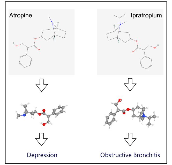
Figure 1: The mapping relationship between molecular conformation and drug efficacy

In this study, we identify two specific manifestations of structural confusion that lead to reduced accuracy. The first is that molecules with similar 2D structures but different 3D geometric structures are problematic because molecular reactions and bindings primarily occur in three-dimensional space. The limitations of 2D structures prevent us from accurately modeling the spatial relationships and interaction forces between molecules, thereby affecting the accuracy of medication recommendations. The second issue is that molecules segmented into smaller substructures do not represent the actual molecular states; they lose their original integrity and stability, and their 3D structures cannot be accurately reproduced in three-dimensional space. The molecular representations expressed by these substructures are also incomplete and inaccurate. Figure 1 shows the mapping relationships of molecular conformations, where even the same 2D molecular structures lead to different efficacies due to minor variations in 3D spatial configurations. We believe that by incorporating the atomic geometric configuration of molecules and completing the 3D information of substructures through comparative learning between bimolecular modalities, we can enhance the overall capability of medication recommendation.

Following this line, we design the BiMoRec model, which addresses the confusion of 2D molecular structures and the inability of substructures to represent true molecular states. Initially, we devise a bimodal graph comparative learning phase, where the bimodal data of molecules serve as input. The 2D modality, through the GIN network, obtains low-dimensional structural embeddings of the molecules, while for the 3D modality, we first acquire each molecule’s 3D data structure using the SDF description file of the molecule, and simultaneously complete the 3D description for the segmented substructures. Subsequently, through the atomic geometric vector machine (GVP) [11], we obtain high-dimensional structural embeddings of the molecules. We then compare the mutual information between the two modal graphs [4], integrating the information of both modalities, allowing the 2D encoder to learn the high-dimensional structural representations of 3D. After completing the comparative learning, we proceed to study the correlation between a given patient’s health condition and the bimolecular granular structure, and finally, by capturing the superficial correlations of medications through the patient’s medication history, we correct any deviations in the recommendation results. Through cross-layer synergistic enhancement, this process yields more accurate and safer medication combinations.

Compared to the latest methods, our model’s introduction of the 3D molecular modality not only completes the molecular structural representation but also employs a pre-trained module with parameters learned in advance. This does not affect the performance of subsequent stages, thereby achieving a balance between accuracy and speed, effectively reducing time costs. Moreover, this module is highly extensible and can be integrated with any medication recommendation framework that utilizes molecular knowledge.

Specifically, the main contributions of this paper can be summarized as follows:

• We introduce the high-dimensional 3D structure of molecules and complete the 3D information of substructures. By using bimodal graph contrastive learning to integrate the knowledge of both modalities, it effectively corrects the structural confusion problem and optimizes the representation space of molecules.

• To improve accuracy and safety, we obtain key substructure sequences through single interactions between patient and molecule, and perform molecular distillation through the latest visit to derive the recommended medication combinations. This approach ensures safety by leveraging both molecular knowledge and historical information.

• We conduct extensive experiments on real datasets MIMIC-III and MIMIC-IV, demonstrating that our proposed method outperforms existing methods.

Below, we provide an overview of the different sections of the paper: (1) Introduction: Introduces the main innovations and the motivation behind this work. (2) Related Work: Summarizes typical studies and current hotspots in medication recommendation fields. (3) Methods: Presents the core ideas of the model and the specific details of its implementation. (4) Experiments: Describes the experimental background, baselines, testing methods, and specific experimental results. (5) Discussion: Delves into an analysis of the experimental results and proposes a series of supportive experiments. (6) Conclusion: Summarizes the research findings and offers perspectives on future research directions.

2 Related Works

In this section, we will introduce the related work from three aspects: medication recommendation, 3D molecular representation, and multi-modal molecules.

2.1 Medication Recommendation

The field of medication recommendation has developed rapidly in recent years, with its primary objective being to provide the most suitable medication combination based on the patient’s specific condition.

Early works in medication recommendation like [34] are instance-based, prescribing on single-visit data, and viewing medication recommendation as a multi-instance and multi-label classification task. After that, studies like [7] employ sequential models to integrate longitudinal visit data. Recently, the research falls into three categories. The first category of work, exemplified by studies like [15, 36, 16], treats medication recommendation as a package, sequence, and other mature recommendation tasks, utilizing advanced algorithms to enhance model quality. The second category of work integrates techniques from other fields, such as [31, 29, 37]. They combine the task of medication recommendation with translation models, generative models, or technologies from other domains, achieving a method that transforms patient states into medication combinations. The third category of work, such as [23, 32, 33, 3], incorporates external knowledge related to medications to fill the knowledge gaps in the data, thereby achieving more accurate representations of medications.

2.2 3D Molecular Representation

In recent years, researchers have begun to realize the importance of 3D geometric information for molecular representation learning. Initially, convolutional layers with continuous filters were used to simulate quantum interactions within molecules, providing valuable insights for subsequent research [22]. Later, researchers began designing more complex network architectures, utilizing spherical harmonics to construct filters and creating rotation- and translation-equivariant neural networks [25], which improved the accuracy and stability of molecular representation. Recently, researchers have started to explore the use of spherical coordinates to capture molecular geometric information or introduce equivariant networks into 3D molecular representation learning [26], ensuring that molecular representations remain equivariant under continuous 3D rotations and translations, further enhancing their robustness and generalization ability. In addition to improving network architectures, researchers have also begun to incorporate physical quantities such as interatomic distances and bond angles into network design, providing a better understanding of the intrinsic structure and properties of molecules.

2.3 Multi-Modal Molecules

In the field of multi-modal molecular learning, 2D graph structures and 3D geometric structures can be viewed as different perspectives of the same molecule. Inspired by contrastive pre-training methods in the vision domain, many research efforts have begun to explore how to use 2D and 3D information jointly for molecular pre-training. For example, using two encoders to separately encode 2D and 3D molecular information while maximizing the mutual information between their representations [24]. Alternatively, pre-training 2D and 3D encoders through contrastive learning and reconstruction [18]. Recent studies have unified the aforementioned 2D and 3D pre-training methods and proposed a 2D graph neural network model [38] that can be enhanced by 3D geometric features.

Our research aims to integrate molecular multi-modality without compromising the efficiency and complexity of the recommendation system, in order to address the issue of structural confusion in medication recommendation and significantly improve existing models.

3 Problem Definition

3.1 Medical Entity

This article introduces the concept of medical entities, which represent relatively comprehensive medical concepts in medical data. In this study, medical entities primarily include three types: diseases, surgeries, and medications, denoted as $\mathcal{D}=\{d_{1},d_{2},\ldots\}$, $\mathcal{P}=\{p_{1},p_{2},\ldots\}$, and $\mathcal{M}=\{m_{1},m_{2},\ldots\}$, respectively. Additionally, molecular modal data is derived from external knowledge and thus does not belong to medical entities.

3.2 Input and Output

The model utilizes Electronic Health Record (EHR) as the data source, encompassing extensive records of patient visits and treatments. Each patient record is represented as $\mathcal{H}$, containing multiple visit records $\mathcal{H}=\{v_{1},v_{2},\ldots,v_{t}\}$, where $v_{t}$ corresponds to the clinical information related to the $t_{th}$ visit. Each visit includes three elements: $\mathcal{D}_{t}\in\{0,1\}^{|\mathcal{D}|},\mathcal{P}_{t}\in\{0,1\}^{\mathcal{P}|},\mathcal{D}_{t}\in\{0,1\}^{|\mathcal{M}|}$, all of which are represented using multi-hot encoding. The output of the model is denoted as $\hat{\mathcal{M}}_{t}$, which is the predicted medication combination for the visit $v_{t}$.

3.3 DDI Matrix

Drug-Drug interactions are a focal point in the field of medication recommendation, as they indicate that certain drug combinations may pose validated safety risks to patients. By excluding drug combinations with safety risks, adverse events caused by such interactions can be reduced, thereby enhancing the safety of drug therapy. The real-world DDI rate is about 0.06. Our DDI information is extracted from the Adverse Event Reporting Systems [9]. We represent DDI information using a binary matrix ${\mathbf{M}^{ddi}}\in\{0,1\}^{|\mathcal{M}|\times|\mathcal{M}|}$, where $\mathbf{M}^{ddi}_{ij}=1$ indicates the presence of an interaction between $m_{i}$ and $m_{j}$. A high frequency of DDI suggests potential safety issues in recommended results.

4 Methods

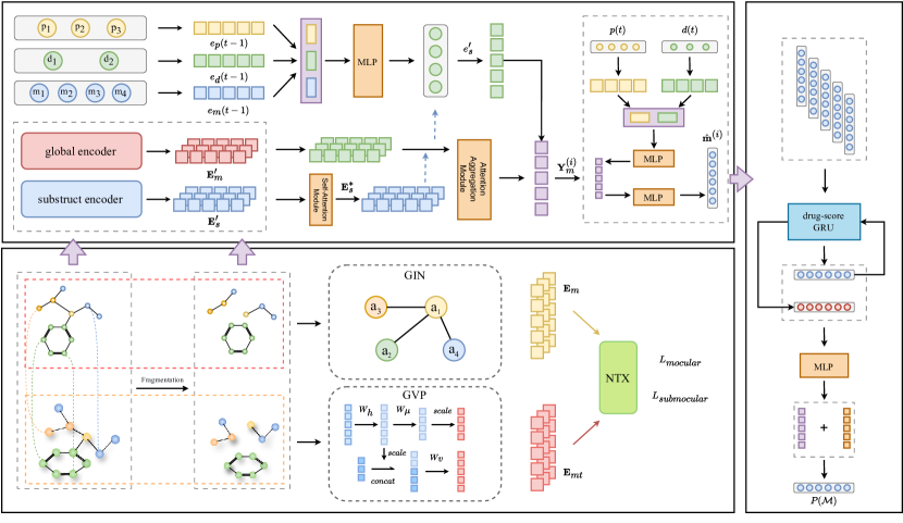
Figure 2: The bottom left of the diagram shows the pre-training and integration process of the bimodal molecular structures, the results of which are applied to the downstream tasks depicted in the top left. The top left section explains how molecular knowledge and patient representations are integrated across layers. This is done to recommend medication combinations at the granularity of single visits, thereby achieving deep knowledge interaction and distilling and extracting molecular substructures at each time point.The right side of the diagram models the sequential relationships of the interaction results and maps them to recommendation probabilities, ultimately yielding the final recommendation results.

Figure 2 illustrates our model, which is comprised of four main components.

(1) In the pre-training stage, by integrating the structural information of molecular bimodal, utilizing contrastive learning, we can obtain the molecular encoding module fused with bimodal structural knowledge, and the substructure encoding module. It can also be understood as learning from the 3D modal teacher model to inject knowledge into the 2D modal model.

(2) In the molecular multi-distillation stage, our objective is to derive single-visit representations of the patient from clinical records. Using the encoders obtained during the pre-training phase, we encode the molecules and their substructures of the medications. Through the collaborative enhancement of deep knowledge and shallow representations, we obtain medication combination results across multiple visits, and based on the current patient’s status, we acquire medication recommendation results under different temporal contexts.

(3) In the stage of recommendation path fusion, our goal is to integrate the sequential relationships of medication recommendations at different time points to obtain the sequence of multiple recommendation results. Subsequently, based on the results of the fusion of multiple time-series environments, we adjust the probability bias for each medication according to the patient’s current health condition, thereby recommending medications that exceed a predetermined threshold.

4.1 Pre-training

In this phase, our aim is to integrate the bimodal structure of molecules, which involves the representation of 2D and 3D structures as well as mutual information learning.

In terms of embedding representations, 2D modal data utilizes Graph Neural Networks (GNN) to encode the molecular structure of drugs and obtain holistic-level representations. GNN iteratively updates node features by aggregating features of neighboring nodes, i.e., updating representations of atomic nodes through specific aggregation strategies. In general, we have:

$$\mathbf{a}^{(k)}(u)=\mathrm{AGG}^{(k)}\left(\left\{\mathbf{f}_{n}^{(k-1)}(v),\mathbf{f}_{e}(u,v)|v\in\mathcal{N}(u)\right\}\right),$$ (1)

$$\mathbf{f}_{n}^{(k)}(u)=\mathrm{COMBINE}^{(k)}\left(\mathbf{a}^{(k)}(u),\mathbf{f}_{n}^{(k-1)}(u)\right),$$ (2)

where $\mathbf{f}_{n}^{(k)}(u)$ is the node feature of node $u$ in the $k$-th layer, $\mathbf{f}_{n}^{(0)}(u)$ is the initial feature of node $u$, $\mathbf{f}_{e}(u,v)$ is the edge feature of edge $(u,v)$, and $\mathcal{N}(u)$ denotes the neighbor of node $u$ on the graph.

A drug molecule is composed of atoms and bonds, and can be represented as a graph $G=(V,E)$, where $V$ is the set of atomic nodes in the molecular graph, and $E$ is the set of chemical bond edges in the molecular graph. Given a molecule $G$, the representation of the entire graph is generated by $L$ layers of GNN, and then aggregated by a readout function to combine all node features in the $L$th layer,

$$\mathbf{f}_{g}(G)=\text{READOUT}\left(\left\{\mathbf{f}_{n}^{(L)}(u)|u\in V\right\}\right).$$ (3)

In this paper, we use GIN [30] as the encoder for drug molecular graphs, which is commonly used in recent work related to drug recommendation and molecular research. We utilize pre-trained encoders as the foundation for subsequent tasks, and the overall-level representations they output are employed for downstream tasks. All drug molecular representations constitute an embedding table $\mathbf{E}_{m}\in R^{|\mathcal{M}|\times h}$, where each row represents a molecular’s representation.

BiMoRec also integrates the 3D modal structure of molecules to enhance molecular representations. Similarly, given the 3D coordinates of an atom, we represent the molecular structure as a graph $\mathcal{G}=(\mathcal{V},\mathcal{E})$, where the nodes $\mathcal{V}$ constitute the set of atoms in the molecule, and we define an edge $\mathcal{E}$ if the distance between atoms is less than 4.5 Å. We directly utilize the 3D coordinates of atoms or edges as node features and edge features. In graph $\mathcal{G}$, we associate each node and edge with geometric features such as 3D coordinates, as well as scalar features describing chemical properties. Thus, we employ dedicated Geometric Vector Perceptrons (GVPs) to construct the molecular structure. Its main advantage lies in its design specifically considering 3D data, enabling direct learning of structural representations from raw atomic coordinates without the need to construct features that are invariant to rotation and translation.

In model construction, we use the tuple $\mathbf{v}_{i}=(\mathbf{v}^{v}_{i},\mathbf{v}^{s}_{i})$ to represent the vector features and scalar features of atom $i$ separately, where $\mathbf{v}^{v}_{i}\in\mathbb{R}^{\mu\times 3}$ is a list of vector features in $\mathbb{R}^{3}$, and $\mathbf{v}^{s}_{i}\in\mathbb{R}^{\nu}$ is a list of scalar features ($\mu$ and $\nu$ are the number of vector features and scalar features, respectively). The edge feature $\mathbf{e}_{ij}=(\mathbf{e}^{v}_{ij},\mathbf{e}^{s}_{ij})$ of edge $(i,j)$ has a similar meaning. The molecular GVP transforms node and edge features through $L$ graph convolution layers to obtain the representation of the input molecule. Specifically, in the $i$th layer, each node aggregates embeddings from neighboring nodes and edges, and then updates its own representation:

$$\mathbf{h}_{i}^{(\ell)}=\mathbf{h}_{i}^{(\ell-1)}+g\Bigg{(}\mathbf{h}_{i}^{(\ell-1)}+\frac{1}{|\mathcal{N}(i)|}\sum_{j\in\mathcal{N}(i)}\mathbf{m}_{ji}^{(\ell)}\Bigg{)},$$ (4)

In this context, $g(\cdot)$ denotes a sequence of three GVP layers, and $\mathcal{N}(i)$ represents the set of neighboring nodes of node $i$ in $\mathcal{G}$. The embedding of node $i$ at layer $\ell$ is $\mathbf{h}^{(\ell)}_{i}$ (specifically, at layer 0, $\mathbf{h}^{(0)}_{i}=\mathbf{v}_{i}$). The message from node $j$ to node $i$ is $\mathbf{m}^{(\ell)}_{ji}$, computed using another sequence of GVP layers: $\mathbf{m}^{(\ell)}_{ji}=g(\text{concat}(\mathbf{h}^{(\ell-1)}_{j},e_{ji}))$, where $\text{concat}(\cdot)$ denotes the concatenation operation of two embeddings. After the final layer of molecular GVP, we also apply a global additive pooling operation to aggregate all node representations into the scalar representation $\mathbf{h}_{d}\in\mathbb{R}^{128}$ of the input drug, obtaining the 3D embedding matrix $\mathbf{E}_{mt}$ of the molecule, where each row represents a molecule’s representation.

Contrastive learning achieves two objectives. The first objective is to make molecules with the same index $i$ increasingly similar. The second objective is to enforce differences between negative samples $\mathbf{E}^{(i)}_{a}$ and $\mathbf{E}^{(k)}_{b}$, where $i\neq k$. If the 2D and 3D representations in a batch come from different molecules, their representations should differ. We use the currently popular NTXent loss to jointly optimize our model:

$$\mathcal{L}=-\frac{1}{N}\sum_{i=1}^{N}\left[\log\frac{e^{sim(\mathbf{E}^{(i)}_{a},\mathbf{E}^{(i)}_{b})/\tau}}{\sum_{k\neq i}^{N}e^{sim(\mathbf{E}^{(i)}_{a},\mathbf{E}^{(k)}_{b})/\tau}}\right]$$ (5)

where $sim(\mathbf{E}_{m},\mathbf{E}_{mt})=\mathbf{E}_{m}\cdot\mathbf{E}_{mt}/(\|\mathbf{E}_{m}\|\|\mathbf{E}_{mt}\|)$ is the cosine similarity and $\tau$ is a temperature parameter which can be seen as weight for the most similar negative pair.

For molecular substructures, existing work demonstrates that the properties of drug molecules partially depend on specific substructures, and the treatment of a patient’s disease also relies on the functions of certain substructures. Our goal is to reconstruct the 3D structures of substructures to make them closer to the actual molecular structures. We first use the BRICS [33] method to decompose drug molecules into substructures, and then complete the 3D information of the substructures using the API provided by RDKit. We decompose all drug molecules to obtain a substructure set $\mathcal{S}$, and finally obtain the embedding matrices of the two different modalities of the structures $\mathbf{E}_{s},\mathbf{E}_{st}\in\mathbb{R}^{|\mathcal{S}|\times h}$, where each row represents the embedding of a specific substructure.

4.2 Molecular Multi-Distillation

At this stage, our goal is to achieve synergistic enhancement between deep molecular knowledge and shallow patient representations. Based on the most recently accessed patient status, we obtain the current patient’s weights for drug molecules and their structures under different temporal conditions, resulting in interaction outcomes in various temporal environments.

We encode the current diagnoses, surgeries, and medications as the health environment of the patient at the current time sequence. We first extract the sets of procedures, diagnoses, and medications at each time point from the visit $v(t-1)$: $d(t-1)=\{d_{i},d_{j},\ldots\}$, $p(t-1)=\{p_{i},p_{j},\ldots\}$, and $m(t-1)=\{m_{i},m_{j},\ldots\}$, all of which are multi-hot vectors mentioned in our problem definition. We define three learnable embedding matrices, $\mathbf{E}_{d}$, $\mathbf{E}_{p}$, and $\mathbf{E}_{me}$, corresponding to diagnoses, surgeries, and medications, where dim is the embedding size. We generate $\mathbf{e}_{d_{i}}$, $\mathbf{e}_{p_{i}}$, and $\mathbf{e}_{m_{i}}$ by mapping diagnoses $d_{i}$, surgeries $p_{i}$, and medications $m_{i}$ to the embedding space, and use them as entity-level representations shared globally for downstream tasks. We obtain the set representations $e_{d}(t)$, $e_{p}(t)$, and $e_{m}(t)$ by mapping all diagnoses, surgeries, and medications through their corresponding embedding matrices.

$$e_{d}(t-1)=d(t-1)E_{d},$$ (6)

$$e_{p}(t-1)=p(t-1)E_{p},$$ (7)

$$e_{m}(t-1)=m(t-1)E_{m}.$$ (8)

Finally, we concatenate the three vectors of equal length, resulting in a single vector with three times the original length, forming the visit-level representation at time $t-1$, $e_{v}^{\prime}(t)\in R^{1\times 3dim}$.

$$e_{v}^{\prime}(t-1)=\mathrm{CONCAT}(e_{d}(t-1),e_{p}(t-1),e_{m}(t-1)).$$ (9)

Then, a multi-layer perceptron(MLP) converts the dimension of the vector $e_{v}^{\prime}(t-1)$ to $|\mathcal{S}|$, the total number of molecular substructures, and a sigmoid function determines the degree to which each substructure is relevant at the current time.

$$e_{s}^{\prime}=\mathrm{MLP}(e_{v}^{\prime}(t-1))$$ (10)

Relying solely on information from a single visit is unwise. For patients with a history of chronic illness, their medical history includes health statuses at different times and the historical progression of their condition, which are potential factors that must be considered. Previous work typically explicitly models the information contained in patient visit sequences when generating patient representations. Innovatively, we perform visit-level interactions between patient representations at each time point and the embedding matrix of the molecular structure encoder, thereby fully preserving the weight of each patient’s demand for drug molecules at each time point. We then correct biases based on the most recent patient representation at visit $t$, ultimately obtaining drug combinations linked to the latest patient visit across various time points.

We use the molecular structure encoder trained during the pretraining phase to encode molecular structures and their substructures, obtaining $\mathbf{E}^{\prime}_{s}$ and $\mathbf{E}^{\prime}_{m}$. For substructures, since the function of molecules is realized through a set of substructures, we need to model the interaction information of substructures. Therefore, we design a substructures self-attention(SSA) module to achieve this goal. We use the embedding matrix $\mathbf{E}_{s}$ of all substructures as input to establish an attention mechanism between each substructure, and finally output an embedding matrix of equal size $\mathbf{E}^{*}_{s}\in\mathbb{R}^{|\mathcal{S}|\times h}$. The self-attention layer is defined as follows:

$$\mathrm{H=LayerNorm(E_{s}+\mathcal{Attn}_{self}(E_{s})),}$$ (11)

$$\mathrm{E_{s}^{*}=SSA(E_{s})=LayerNorm(H+MLP(H)),}$$ (12)

$\mathcal{Attn}_{self}$ denotes the self-attention mechanism defined by the following formula:

$$\mathcal{Attn}_{self}(\mathrm{X})=\mathrm{Softmax}\left(\frac{\mathcal{Q}_{x}\mathcal{K}_{x}^{\top}}{\sqrt{d_{k}}}\right)\mathcal{V}_{x},$$ (13)

where $d_{k}$ is the dimension of the key embeddings, and $\mathbf{Q}_{x}$, $\mathbf{K}_{x}$, and $\mathbf{V}_{x}$ are the query, key, and value matrices of the input $\mathbf{X}$.

We perform attention aggregation on the overall molecular representation $\mathbf{E}^{\prime}_{m}$ and the substructure interaction representation $\mathbf{E}^{*}_{s}$, using a mask matrix to rescale the attention matrix when calculating the attention coefficients.

$$\mathcal{Attn}_{mol-sub}(\mathrm{X,Y})=\mathrm{Softmax}\left(\frac{\mathcal{Q}_{x}\mathcal{K}_{y}^{\top}}{\sqrt{d_{m}in}}\right),$$ (14)

$$\mathcal{Attn}_{mol-sub}(\mathrm{X,Y})=\mathrm{mask}(\mathcal{Attn}_{mol-sub},-(1\ll 32))$$ (15)

where $d_{\min}$ is the minimum embedding dimension of $\mathbf{X}$ and $\mathbf{Y}$, $\mathbf{Q}_{x}$ and $\mathbf{K}_{y}$ are the query and key matrices of the input, and the mask function replaces the set of substructures without mapping relationships with the minimum value.

$$\forall s\in S_{k},\tilde{\mathbf{y}}_{s}^{(i)}=\mathbf{e}_{s}^{\prime(i)}\mathbf{y}_{s},$$ (16)

where $\mathbf{e}_{s}^{\prime(i)}$ is the element of $\mathbf{e}_{s}^{\prime}$ corresponding to the substructure $s$. Finally, we obtain the perception representation of the substructure at the current time sequence through the attention matrix.

$$\ddot{\mathbf{y}}_{k}^{(i)}=\sum_{s\in S_{k}}\mathcal{Attn}_{mol-sub}\tilde{\mathbf{y}}_{s}^{(i)}.$$ (17)

Finally, we obtain all the aggregated substructure embedding representations $\mathbf{Y}_{m}^{(i)}$.

To relate the aggregated substructure embeddings to the patient’s latest health status, we use the most recent patient visit as the basis for bias correction. Through an MLP layer, we obtain the weights of the latest patient representation for the elements of the substructure set, thereby calibrating the substructure embeddings.

$$e_{d}(t)=d(t)E_{d},e_{p}(t)=p(t)E_{p},$$ (18)

$$e_{v}^{\prime}(t)=\mathrm{CONCAT}(e_{d}(t),e_{p}(t)),$$ (19)

$$\mathbf{W}_{m}=\sigma(\mathrm{MLP}(e_{v}^{\prime}(t))).$$ (20)

$\mathbf{e}_{d}(t)$ and $\mathbf{e}_{p}(t)$ are the diagnostic and surgical embedding representations of the patient’s most recent visit. By concatenating these embeddings and passing them through an MLP layer, we obtain the desired weight vector $\mathbf{W}_{m}$. Finally, we correct the substructure embedding matrix by multiplying it with a diagonal matrix, and then scale the dimensions through an MLP network to obtain the representation $\hat{\mathbf{m}}^{(i)}$ for each drug.

$$\hat{\mathbf{m}}^{(i)}=\mathrm{MLP}(\mathbf{W}_{m}\mathrm{Y}_{m}^{(i)}).$$ (21)

This stage’s results prepare for the next phase of the task.

4.3 Fusion of Drug Evolution Trajectories

The purpose of this stage is to integrate the drug representations obtained for the patient at each time point. This representation results from the interaction of deep and shallow knowledge and subsequent bias correction, ultimately yielding the recommendation probabilities for all drugs.

By embedding the multiple drug representations generated in the previous stage $\{\hat{\mathbf{m}}_{v_{1}},\hat{\mathbf{m}}_{v_{2}},\ldots,\hat{\mathbf{m}}_{v_{t-1}}\}$ and inputting them into a gated recurrent unit $\text{GRU}(\cdot)\in\mathbb{R}^{|\mathcal{M}|}$ to model the sequential relationships, we then process the outputs through a multilayer perceptron

$$\text{MLP}(\cdot)\colon\mathbb{R}^{|\mathcal{M}|\times 2}\to\mathbb{R}^{|\mathcal{M}|}.$$

Finally, we concatenate the results with the patient’s most recent representation to generate the final drug probabilities.

$$\mathbf{o}_{v_{t-1}}=\text{GRU}(\mathbf{o}_{v_{t-2}},\mathbf{h}_{v_{t-1}}),$$ (22)

$$P(\mathcal{M})=\sigma(\text{MLP}(o_{v_{t-1}}+e_{v}^{\prime}(t)))$$ (23)

where $\mathbf{o}_{v_{t-2}}$ is the intermediate variable generated by $GRU(\cdot)$, and we represent $\mathbf{o}_{v_{0}}$ as a zero vector. Finally, we use a nonlinear activation function $\sigma$ to convert the input representation into the predicted probability $P(\mathcal{M})$ for each drug $M_{i}$.If the probability exceeds a certain threshold $\delta$, the drug recommendation is accepted; otherwise, it is not. Finally, we obtain the prediction results $\hat{m}_{i}$ for each medication.

4.4 Model Training

Medication recommendation is essentially a multi-label binary classification task. Therefore, we use the binary cross-entropy loss function $L_{bce}$ and the multi-label margin loss function $L_{multi}$. Additionally, due to the specific nature of drug recommendation, we use the drug DDI loss function $L_{ddi}$ [33], which calculates the probability of DDI occurrence by identifying drug pairs with potential DDI risk in the drug combination. The definitions of the three loss functions are as follows:

$$\mathcal{L}_{bce}=-\sum_{i=1}^{|\mathcal{M}|}{m_{i}}\log({\hat{m}_{i}})+(1-{m_{i}})\log(1-{\hat{m}_{i}}),$$ (24)

$$\mathcal{L}_{multi}=\sum_{i,j:{m_{i}}=1,{m_{j}}=0}\frac{\max(0,1-({\hat{m}_{i}}-{\hat{m}_{j}}))}{|\mathcal{M}|},$$ (25)

$$\mathcal{L}_{ddi}=\sum_{i=1}^{|\mathcal{M}|}\sum_{j=1}^{|\mathcal{M}|}\mathbf{M}^{ddi}_{ij}\cdot{\hat{m}_{i}}\cdot{\hat{m}_{j}},$$ (26)

where $m_{i}$ represents the true value of the $i$th medication during the current visit, while $\hat{m}_{i}$ represents the model’s predicted value for the $i$th medication, both of which are binary variables.

Although DDI indicates the potential risk of drug combinations, considering medical practice, certain adverse reactions are acceptable. Pursuing the lowest DDI rate without considering efficacy does not lead to the best drug combination. Therefore, we must set a threshold for DDI; if this threshold is exceeded, the weight of DDI increases. When using the composite loss function, we adopt the same research methodology as before [33] to balance the accuracy and safety of the drug combinations.

$$\mathcal{L}=\alpha(\beta\mathcal{L}_{bce}+(1-\beta)\mathcal{L}_{multi})+(1-\alpha)\mathcal{L}_{ddi},$$ (27)

$$\alpha=\begin{cases}1&\rho<\phi\\ \min\{1,\exp(\tau(1-\frac{\rho}{\phi}))\}&\rho\geq\phi\end{cases},$$ (28)

where $\beta$ is hyperparameters, and the controllable factor $\alpha$ is relative to DDI rate, $\phi\in(0,1)$ is a DDI acceptance rate, $\rho$ is the current DDI rate and $\tau$ is a hyper-parameter.

5 Experiments

This section primarily introduces the experimental setup, including model configurations and parameter selections, as well as evaluation metrics. Additionally, it presents a series of comparison results between the baseline models and our model.

5.1 Setup Protocol

First, we provide a detailed description of the experimental setup, including the environmental configuration, parameter selection, basic model configuration, and sampling methods used during the testing phase.

5.1.1 Experimental Environment

The experiments are carried out on an Ubuntu 22.04 system equipped with 30GB of memory, 12 CPUs, and a 24GB NVIDIA RTX3090 GPU, utilizing PyTorch 2.0.0 and CUDA 11.7.

5.1.2 Configuration and Parameter

For the embedding matrices of entities $E_{d}$, $E_{p}$, and $E_{m}$, we use $\text{dim}=128$ as the embedding size, initialized between -0.1 and 0.1. For the molecular GNN, we use a 4-layer GIN with a hidden size of 128. For each molecular graph, the initial 9-dimensional node features include atom count, chirality, and other additional atomic features. The 3-dimensional edge features include bond type, bond stereochemistry, and conjugated bonds. The molecular 3D features include molecular conformations, 3D coordinates, RBF distances, and normalized interatomic vectors. We also use a 3-layer GVP, where the hidden dimensions for node feature scalars and vectors are 128 and 64, respectively, and the hidden dimensions for edge feature scalars and vectors are 32 and 1, respectively. For the GRU, we use the same number of hidden units as the number of drugs. For the loss functions, we set the thresholds $\delta=0.5$, $\tau=2.5$, $\beta=0.95$, and $\phi=0.06$. We train for 300 epochs during the pretraining stage and 20 epochs during the training stage.

5.1.3 Sampling Approach

Due to the limited availability of publicly accessible EHR data, we adopt bootstrapping sampling in this phase, following the approach recommended in [32]. This technique is particularly effective in scenarios where sample sizes are small, as detailed in [19] and [8].

5.2 Datasets

Table 1: Statistics of the datasets.

Item	MIMIC-III	MIMIC-IV
# patients	6,350	60,125
# clinical events	15,032	156,810
# diseases	1,958	2,000
# procedures	1,430	1,500
# medications	131	131
avg. # of visits	2.37	2.61
avg. # of medications	11.44	6.66

We use the MIMIC-III [13] and MIMIC-IV [12] datasets, which are derived from clinical data in the intensive care unit (ICU). These datasets include clinical records, physiological measurements, laboratory monitoring data, and medication records of ICU patients. We adopt the same data processing methods as previous studies. The detailed statistics of the processed datasets are shown in the table 1.

5.3 Evaluation Metrics

We delve into the performance evaluation of our method using four principal metrics: Jaccard, DDI rate, F1, and PRAUC. Here’s an in-depth explanation of each metric and its application in our study.

Jaccard (Jaccard similarity score) measures the similarity between two sets by dividing the size of their intersection by the size of their union. In medication recommendation, a higher Jaccard score indicates greater consistency between the predicted drug combination and the actual medication, reflecting higher accuracy.

$$Jaccard(t)=\frac{|\{i:\hat{m}_{i}=1\}|\cap|\{i:{m}_{i}=1\}|}{|\{i:\hat{m}_{i}=1\}|\cup|\{i:{m}_{i}=1\}|},$$ (29)

$$Jaccard=\frac{1}{N_{h}}\sum_{t=1}^{N_{h}}Jaccard(t),$$ (30)

where $\hat{m}_{i}$ represents the multi-hot vector of the predicted outcome, $m_{i}$ represents the real label, $Jaccard(t)$ represents the evaluation result at visit $t$, and $N_{h}$ represents the total number of visits for patient $h$.

DDI (Drug-Drug Interaction rate) measures the incidence of adverse reactions in the recommended combinations. A lower rate indicates higher safety of the drug combinations.

$$DDI=\frac{\sum_{i=1}^{N_{h}}\sum_{k,l\in\{j:\hat{m}_{j}(t)=1\}}1\{a^{ddi}_{kl}=1\}}{\sum_{i=1}^{N_{h}}\sum_{k,l\in\{j:m_{j}(t)=1\}}1},$$ (31)

where $N_{h}$ denotes the total number of visits for patient $h$, $m(t)$ and $\hat{m}(t)$ denote the real and predicted multi-labels at visit $t$, $m_{j}(t)$ denotes the $j^{th}$ entry of $m(t)$, $a^{ddi}$ is the prior DDI relation matrix, and $1$ is an indicator function that returns 1 when $a^{ddi}=1$, otherwise 0.

F1 (F1-score) combines precision and recall, reflecting the model’s ability to accurately identify correct medications while ensuring comprehensive coverage.

$$Precision(t)=\frac{|\{i:\hat{m}_{i}=1\}\cap\{i:m_{i}=1\}|}{|\{i:\hat{m}_{i}=1\}|},$$ (32)

$$Recall(t)=\frac{|\{i:\hat{m}_{i}=1\}\cap\{i:m_{i}=1\}|}{|\{i:m_{i}=1\}|},$$ (33)

$$F1(t)=\frac{2}{\frac{1}{Precision(t)}+\frac{1}{Recall(t)}},$$ (34)

$$F1=\frac{1}{N_{h}}\sum_{i=1}^{N_{h}}F1(i),$$ (35)

where $N_{h}$ represents the total number of visits for patient $h$.

PRAUC (Precision-Recall Area Under Curve) assesses model performance across different recall levels, indicating the ability to maintain model precision with increasing recall.

$$PRAUC(t)=\sum_{k=1}^{|M|}Precision_{k}(t)\triangle Recall_{k}(t),$$ (36)

$$\triangle Recall_{k}(t)=Recall_{k}(t)-Recall_{k-1}(t),$$ (37)

where $|M|$ denotes the number of medications, $k$ is the rank in the sequence of the retrieved medications, and $Precision_{k}(t)$ represents the precision at cut-of $k$ in the ordered retrieval list and $\triangle Recall_{k}(t)$ denotes the change of recall from medication $k-1$ to $k$. We averaged the PRAUC across all of the patient’s visits to obtain the final result,

$$PRAUC=\frac{1}{N_{h}}\sum_{i=1}^{N_{h}}PRAUC(t),$$ (38)

where $N_{h}$ represents the total number of visits for patient $h$.

Avg. # of Drugs (Average number of drugs) measures the average number of drugs in each recommendation result. A higher value indicates that each recommendation contains more drugs, which may increase the complexity of clinical treatment and the risk of adverse reactions. Conversely, a lower value suggests that the drug combinations may be safer and help minimize unnecessary drug use. It is important to note that this metric is for reference only and the size of the combination should not be used as a strict evaluation standard.

$$Avg.\#ofDrugs=\frac{1}{N_{h}}\sum_{i=1}^{N_{h}}|\hat{M}(i)|,$$ (39)

where $N_{h}$ represents the total number of visits for patient $h$ and $|\hat{M}(i)|)$ denotes the number of predicted medications in visit $i$ of patient $h$.

5.4 Baselines

To verify the performance of our model, we chose the following high-performance methods as the baseline model for comparison.

LR (Logistic Regression) is a widely used linear classification algorithm that calculates the probability of an instance belonging to a specific category based on a linear combination of input features. It is commonly used for probability prediction and binary or multi-class classification tasks.

ECC [21] (Ensemble of Classifier Chains) uses a series of interconnected classifiers to improve prediction accuracy, where the output of one classifier serves as the input for the next. This method is suitable for multi-label classification tasks and can effectively enhance the overall performance of the model.

RETAIN [7] is an attention-based model that analyzes patient time series to achieve accurate disease prediction and management. It provides medication recommendations by dynamically capturing key clinical events in a patient’s medical history.

LEAP [34] enhances the effectiveness of medications by modeling label dependencies through decomposing the treatment process into a sequential procedure.

GAMENet [23] is a medication recommendation that integrates the strengths of graph neural networks with memory networks and effectively discerns patterns and temporal sequences within medical data, thereby enhancing the precision of its predictions.

SafeDrug [32] leverages the combination of patients’ health conditions and medication-related molecular knowledge. This approach, by reducing the impact of DDIs, can recommend safer medication combinations.

MICRON [31] recommends medications based on the dynamic changes in a patient’s health condition. It focuses on updating medication combinations according to the patient’s new symptoms to enhance treatment efficacy while reducing potential side effects.

COGNet [29] employs the Transformer architecture for drug recommendations, using a translation approach to infer medications from illnesses. It also features a copy mechanism to integrate beneficial drugs from past prescriptions into new recommendations.

MoleRec [33] delves into the importance of specific molecular substructures in medications. This approach enhances the precision of medication recommendations by leveraging finer molecular representations.

5.5 Performance Comparison

Table 2: The performance of each model on the test set regarding accuracy and safety. The best and the runner-up results are highlighted in bold and underlined respectively under t-tests, at the level of 95% confidence level.

Model	MIMIC-III					MIMIC-IV
	Jaccard$\uparrow$	DDI$\downarrow$	F1$\uparrow$	PRAUC$\uparrow$	Avg.#Med	Jaccard$\uparrow$	DDI$\downarrow$	F1$\uparrow$	PRAUC$\uparrow$	Avg.#Med
LR	0.4924	0.0830	0.6490	0.7548	16.0489	0.4569	0.0783	0.6064	0.6613	8.5746
ECC	0.4856	0.0817	0.6438	0.7590	16.2578	0.4327	0.0764	0.6129	0.6530	8.7934
RETAIN	0.4871	0.0879	0.6473	0.7600	19.4222	0.4234	0.0936	0.5785	0.6801	10.9576
LEAP	0.4526	0.0762	0.6147	0.6555	18.6240	0.4254	0.0688	0.5794	0.6059	11.3606
GAMENet	0.4994	0.0890	0.6560	0.7656	27.7703	0.4565	0.0898	0.6103	0.6829	18.5895
SafeDrug	0.5154	0.0655	0.6722	0.7627	19.4111	0.4487	0.0604	0.6014	0.6948	13.6943
MICRON	0.5219	0.0727	0.6761	0.7489	19.2505	0.4640	0.0691	0.6167	0.6919	12.7701
COGNet	0.5312	0.0839	0.6744	0.7708	27.6335	0.4775	0.0911	0.6233	0.6524	18.7235
MoleRec	0.5293	0.0726	0.6834	0.7746	22.0125	0.4744	0.0722	0.6262	0.7124	13.4806
BiMoMed	0.5409	0.0734	0.6936	0.7832	20.9027	0.4851	0.0704	0.6367	0.7300	13.6222

In this section, we compare our model with baseline models, evaluating the accuracy and safety of the models through fundamental metrics. For baseline methods with a provided test model, we directly use the provided baseline model. For baseline methods without a provided test model, we regenerate the model files through retraining and conduct tests. We use the optimal parameter settings described in their respective papers to obtain results for each baseline method. Table 2 details the comparison results.

Among the various baseline methods, LR and ECC use traditional recommendation methods and perform poorly in terms of accuracy. LEAP decomposes treatment recommendations into a sequential decision process, utilizing sequence relationships to improve effectiveness, but it does not surpass traditional methods. RETAIN also introduces a sequence model but results in an excessively high DDI rate.

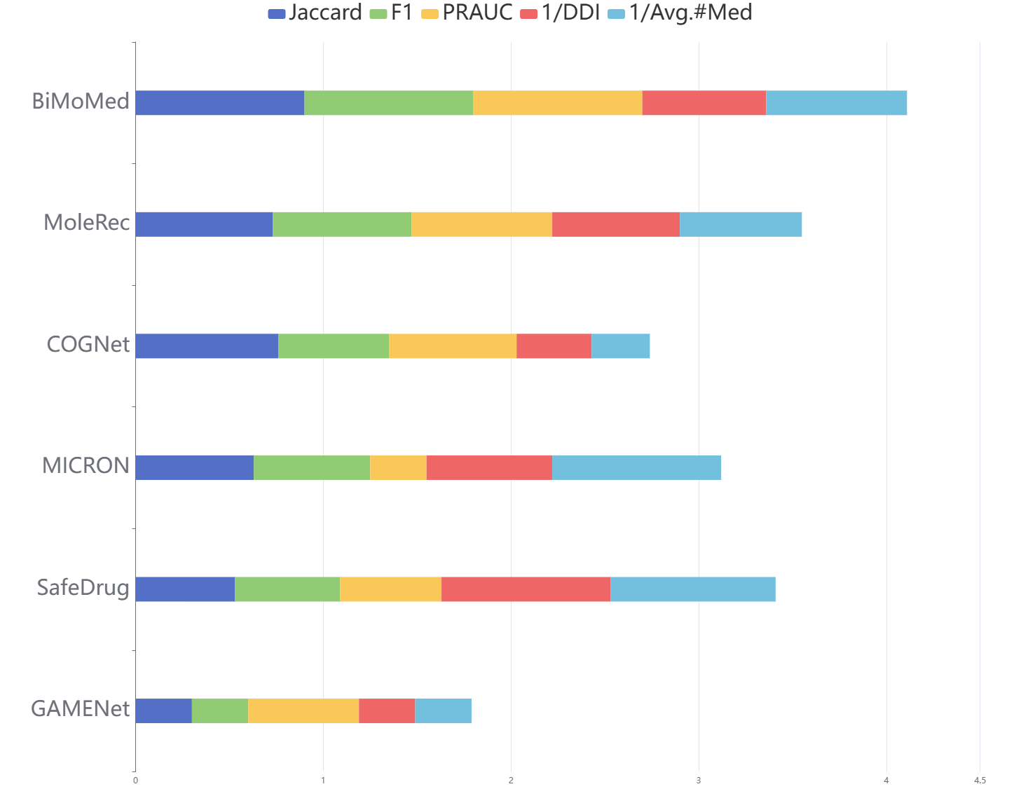
Figure 3: Comparison with recent outstanding works across all metrics in MIMIC-III.

For a more intuitive comparison between the baselines and our model, we integrate all evaluation metrics into a single chart. Jaccard, F1, and PRAUC are used to measure model accuracy, while DDI and Avg.#Med are used to measure safety. We normalize the metrics to the 30%-90% range and display them in Figure 3. It is important to note that the chart does not include the efficiency metrics of the models.

Table 3: The performance of recent excellent models in training and inference efficiency.

method	Convergence Epoch	Training Time /Epoch(s)	Total Training Time(s)	Inference Time(s)
GAMENet	39	45.31	1767.09	19.27
SafeDrug	54	38.32	2069.28	20.15
MICRON	40	17.48	699.20	14.48
COGNet	103	38.85	4001.55	142.91
MoleRec	25	249.32	6233.00	32.10
BiMoRec	15	416.61	6249.15	15.16

Additionally, we compare the operational efficiency of different models, including the training time per epoch, total training time, and inference time for each model, as shown in Table 3.

GAMENet significantly improves model accuracy compared to previous models by integrating patients’ visit history into the model framework without significantly increasing model complexity. However, its DDI rate is too high. SafeDrug significantly reduces the DDI rate by explicitly modeling relationships between medication molecules, but it does not capture relationships between medications and diseases, leaving room for improvement in accuracy. MICRON adjusts recommended medication combinations by capturing changes in patients’ physical conditions between two visits, thereby improving accuracy and training efficiency after certain data filtering. COGNet designs a replication mechanism that significantly improves the Jaccard metric but increases the number of iterations, affecting its time efficiency and failing to ensure the safety of certain medication combinations. MoleRec introduces external knowledge of molecules, constructs relationships between medication molecules and their substructures, and links them with patients’ diseases and surgeries, improving accuracy without severely impacting safety. However, due to the introduction of deep graph networks and message-passing mechanisms, it significantly reduces training speed.

Our model re-calibrates the representation of molecules and their substructures by introducing the 3D modality of molecules, increasing the dimensionality of molecular representation, addressing real structural confusion issues, and designing a substructure distillation mechanism at the access level. This adjusts the interaction mechanism between molecular knowledge and patients’ physical conditions, enhancing model rationality and accuracy while only slightly increasing the DDI rate.

Comparing the operational efficiency of the models, although the training time per epoch for our model is relatively long, the number of epochs required for convergence is significantly shortened during actual training, often requiring only 15 epochs for convergence. Therefore, the total training time is not significantly increased compared to MoleRec.

6 Discussions

In this section, we delve into a detailed analysis of the experimental outcomes previously discussed. Additionally, we carry out a series of supplementary experiments to affirm the comprehensiveness and logic behind our approach, ensuring its robustness and the validity of its advancements in the field.

6.1 Effectiveness Analysis

The above comparative experiments demonstrate the superior performance of our model in terms of accuracy and safety. We will conduct a comprehensive analysis of the experimental results here.

Previous medication recommendation works typically base medication recommendations on the patient’s physical condition. With the introduction of external molecular knowledge, accuracy and safety further improve. However, the introduced molecular structures are merely 2D projections of the actual molecular structures, leading to structural confusion issues. Additionally, molecular substructures do not interact independently with the patient’s single visit state, resulting in a lack of crucial substructure combinations needed for each visit’s medication.

To address the identified issues, we introduce the 3D modality of molecules, filling in the missing three-dimensional information in molecular representation and effectively resolving the structural confusion problem. Simultaneously, we directly interact molecular knowledge with the patient’s single visit representation, obtaining the necessary molecular substructures for each visit. We use the patient’s latest representation as a standard to adjust the weights of the substructures, correcting biases to better utilize the introduced molecular knowledge. Our proposed method addresses issues not discovered by other models, significantly enhancing the rationality and overall performance of the medication recommendation system.

6.2 Efficiency Analysis

To more accurately represent the efficiency of our model, we analyze the time complexity of the model step by step. In the pre-training module, we use GIN and GVP networks to obtain two molecular modalities’ representations, along with two fully connected layers and an NTXent layer. The time complexity of the GNN layer is $O(4\cdot(N+E)^{4})$, where $N$ is the number of nodes and $E$ is the number of edges. The fully connected layer’s time complexity is $O(4\cdot n_{i}\cdot n_{o})$, where $n_{i}$ is the number of input nodes and $n_{o}$ is the number of output nodes. The NTXent layer’s time complexity is $O(n_{i}^{2})$, and in this model, the NTXent layer runs twice, so the total time complexity is $O(2\cdot n_{i}^{2})$. Summarizing the above, the total time complexity of the pre-training is approximately

$$O(4\cdot(N+E)^{4}+4\cdot n_{i}\cdot n_{o}+2\cdot n_{i}^{2})$$ (40)

In the subsequent substructure interaction distillation stage, we use three embedding layers, a GRU layer, a molecular structure and its substructure graph neural network along with the corresponding attention mechanism, and multiple fully connected layers. The time complexity of the embedding layers is $O(3\cdot n\cdot d)$, where $n$ is the length of the input sequence and $d$ is the size of the embedding dimension. The time complexity of the GRU layer is $O(t\cdot h^{2})$, where $t$ is the sequence length and $h$ is the size of the hidden layer. The time complexity of the GNN layer is $O(2\cdot(N+E)^{4})$, where $N$ is the number of nodes and $E$ is the number of edges. The time complexity of the attention mechanism is $O(2\cdot L^{2}\cdot D)$, where $L$ is the length of the input sequence and $D$ is the corresponding dimension. The time complexity of multiple fully connected layers is denoted as $O(\Sigma(n_{i}\cdot n_{o}))$, where $n_{i}$ is the number of input nodes and $n_{o}$ is the number of output nodes. Finally, the overall time complexity is:

$$O(3\cdot n\cdot d+t\cdot h^{2}+2\cdot(N+E)^{4}+2\cdot L^{2}\cdot D+\Sigma(n_{i}\cdot n_{o}))$$ (41)

Through the above calculations, we observe that the number of layers in the GNN network is an important model setting. Although a 4-layer network structure increases the overall runtime of the model, it enables the model to converge quickly. Therefore, the final time efficiency does not decrease as a result.

6.3 Ablation Study

To evaluate the contribution of our innovations to the overall performance of the model and eliminate interference from other factors, we delete key modules and perform logical adjustments to set up several variant experiments.

Table 4: The performance of each ablation model on the test set regarding accuracy and safety. The best and the runner-up results are highlighted in bold and underlined respectively under t-tests, at the level of 95% confidence level.

Model	MIMIC-III					MIMIC-IV
	Jaccard$\uparrow$	DDI$\downarrow$	F1$\uparrow$	PRAUC$\uparrow$	Avg.#Med	Jaccard$\uparrow$	DDI$\downarrow$	F1$\uparrow$	PRAUC$\uparrow$	Avg.#Med
BiMoRec $w/o$ A	0.5356	0.0697	0.6887	0.7823	20.4086	0.4874	0.0673	0.6382	0.7318	14.8917
BiMoRec $w/o$ B	0.5373	0.0727	0.6906	0.7787	22.0278	0.4836	0.0649	0.6346	0.7244	14.8244
BiMoRec $w/o$ A+B	0.5357	0.0672	0.6888	0.7815	22.1939	0.4798	0.0622	0.6307	0.7209	14.7726
BiMoRec	0.5526	0.0684	0.7033	0.7955	22.4693	0.4912	0.0635	0.6419	0.7324	14.8019

BiMoRec $w/o$ A: In this variant, we delete the pre-training module, which means not using the model’s 3D modality data. Like previous work, we use the molecular SMILES strings as the input to the graph neural network to construct the molecular structure and its substructure embeddings.

BiMoRec $w/o$ B: We eliminate the Substructure-Patient Interaction Distillation module in this variant, removing the interaction between substructures and a single patient visit. Instead, we rely solely on the patient’s latest physical condition to interact with the single visit representation, and finally obtain the weights of the medication substructures.

BiMoRec $w/o$ A+B: We simultaneously remove both the pre-training module and the Substructure-Patient Interaction Distillation module. This variant neither integrates the dual modalities of molecular representation nor interacts with the patient’s single representation, relying entirely on the relationships between medications, diseases, and surgeries in patient visits to make recommendations.

As shown in Table 4, the ablation experiment results confirm our expectations. BiMoRec $w/o$ A demonstrates that by introducing the 3D molecular modality, we improve the model’s recommendation accuracy, supplementing the molecular spatial information and resolving the structural confusion issue. We will provide more detailed evidence in subsequent case analyses. BiMoRec $w/o$ B indicates that our Substructure-Patient Interaction Distillation module effectively captures useful medication substructures in each visit, learning the relationships between patient representations and substructures at the visit granularity level. BiMoRec $w/o$ A+B shows a slight improvement in safety but a significant reduction in accuracy. This phenomenon is common in the medication recommendation field, as safety and accuracy often need to balance and constrain each other. The optimal model performance usually results from balancing both. Additionally, the experiment indicates that the dual molecular modalities and the interaction between visit-level molecular and patient representations have a synergistic effect, improving model performance more effectively when used together.

6.4 Parameter Sensitivity

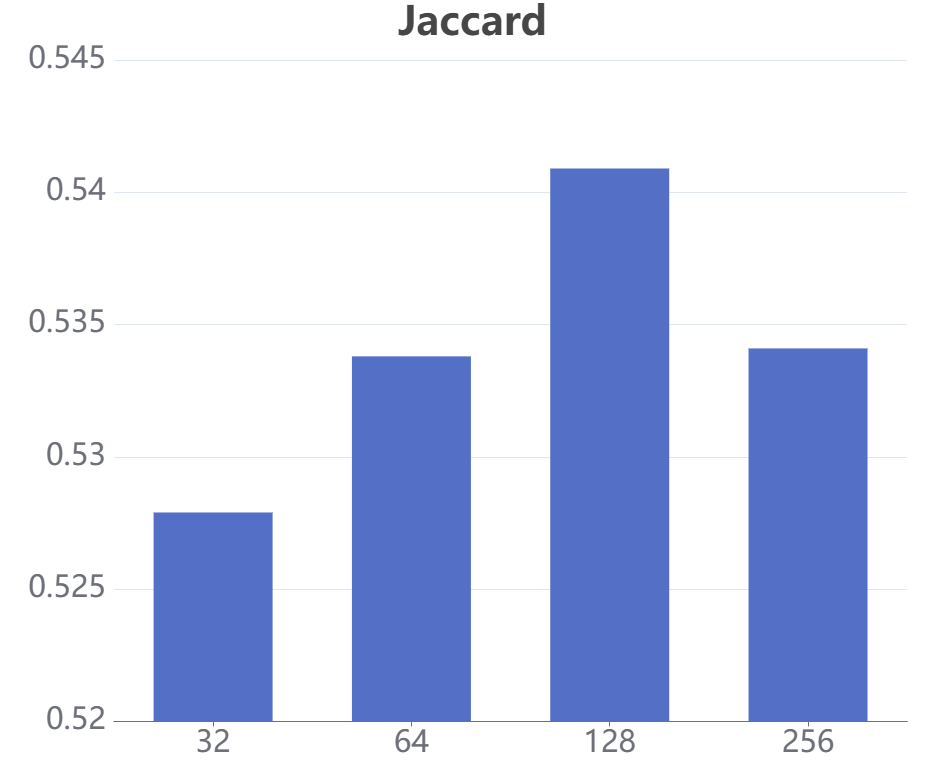
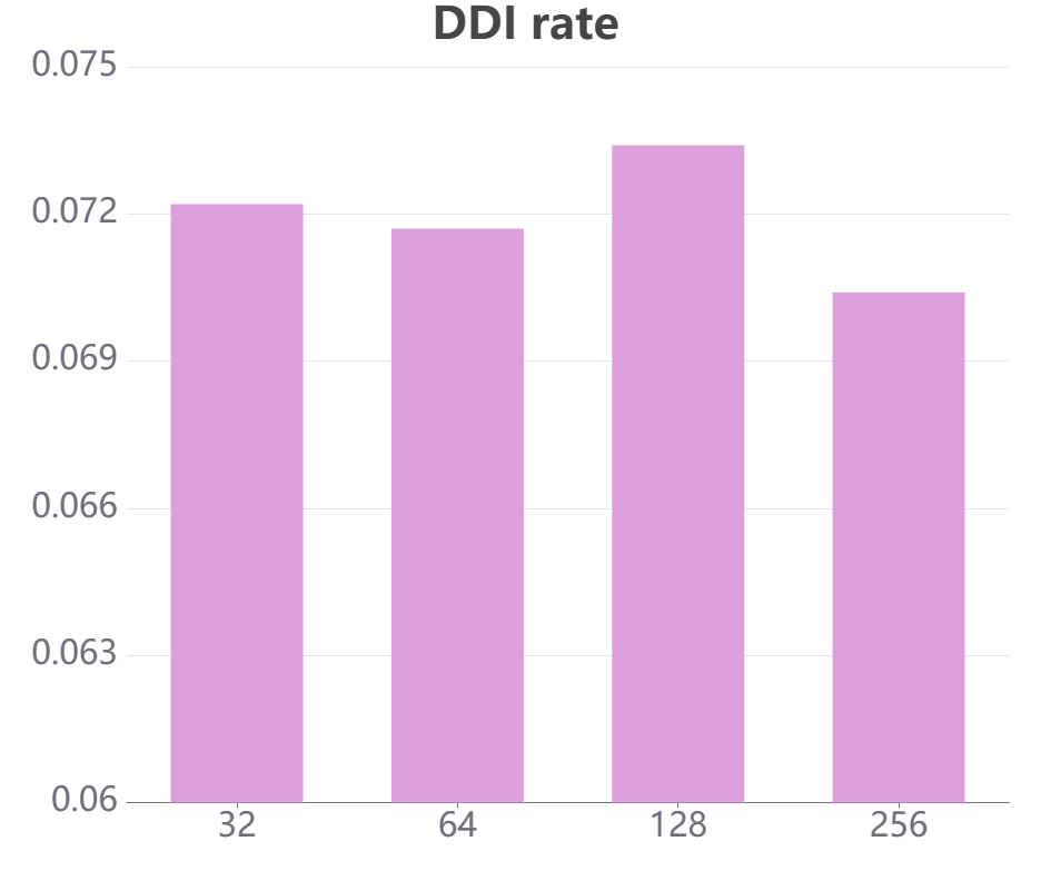
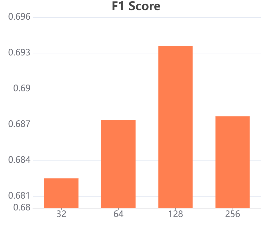
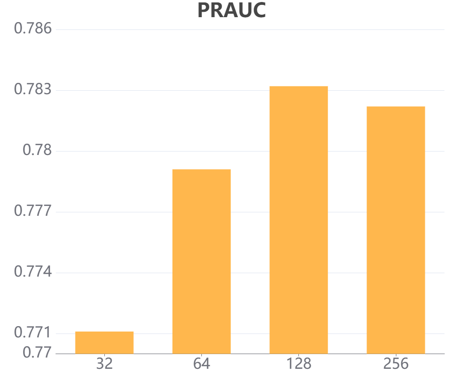
(a) The impact of embedded dimensions on results.

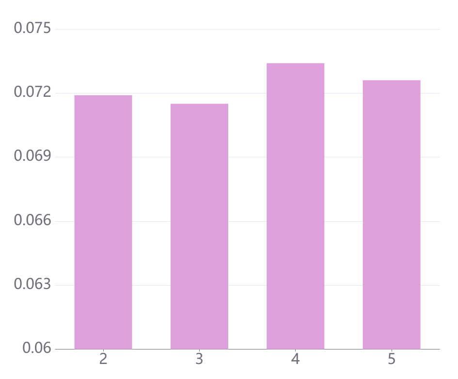
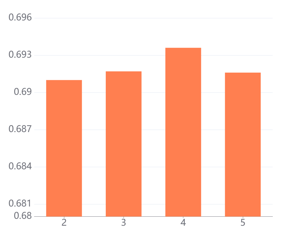
(b) The impact of GNN layers’ number on results.

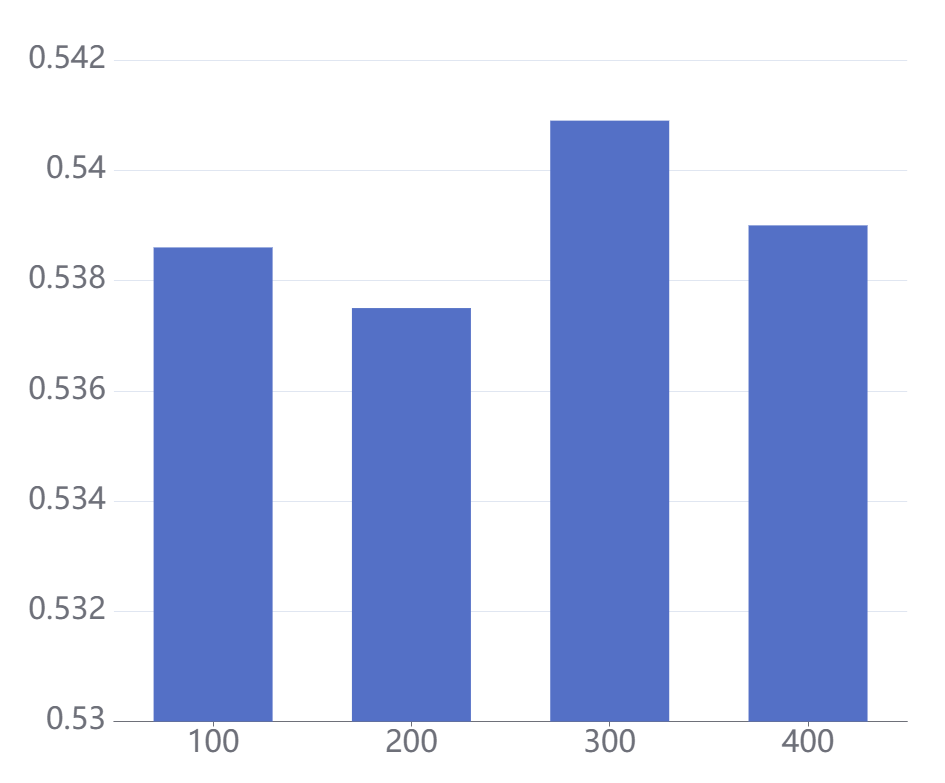
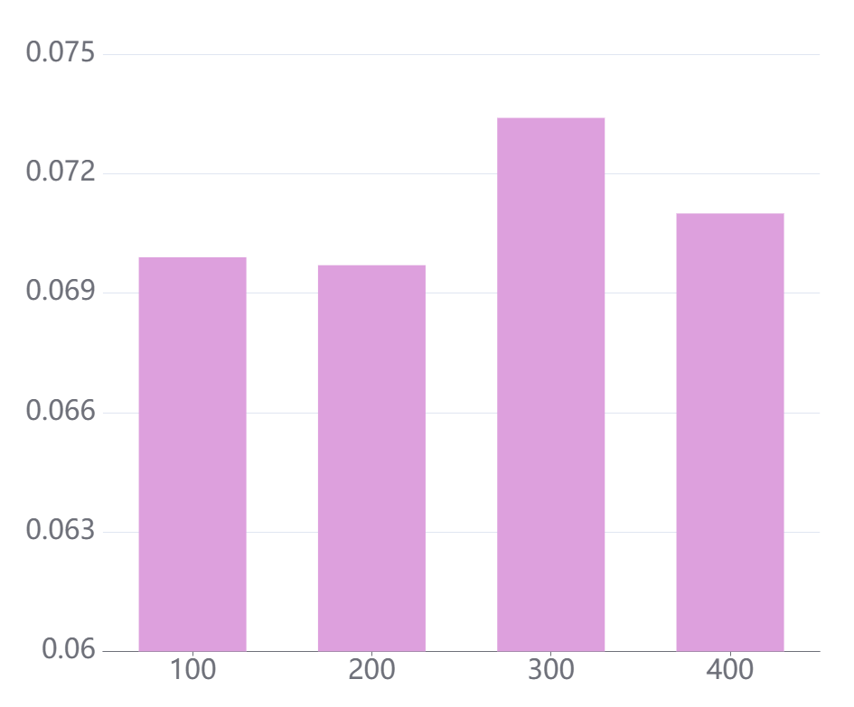
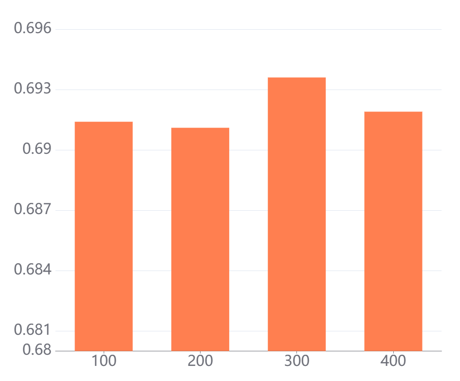
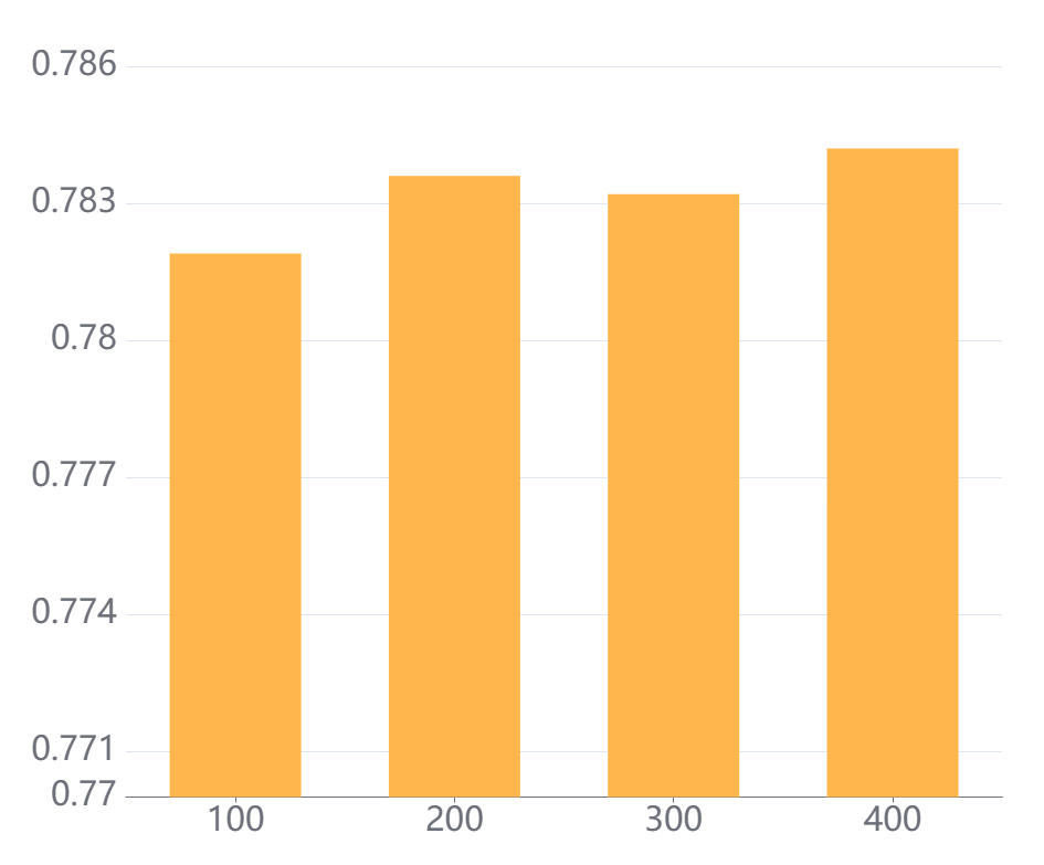
(c) The impact of pre training epochs on results.

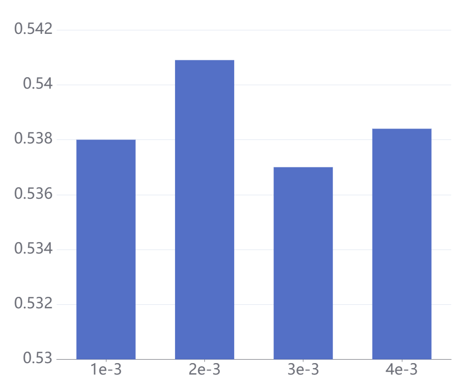
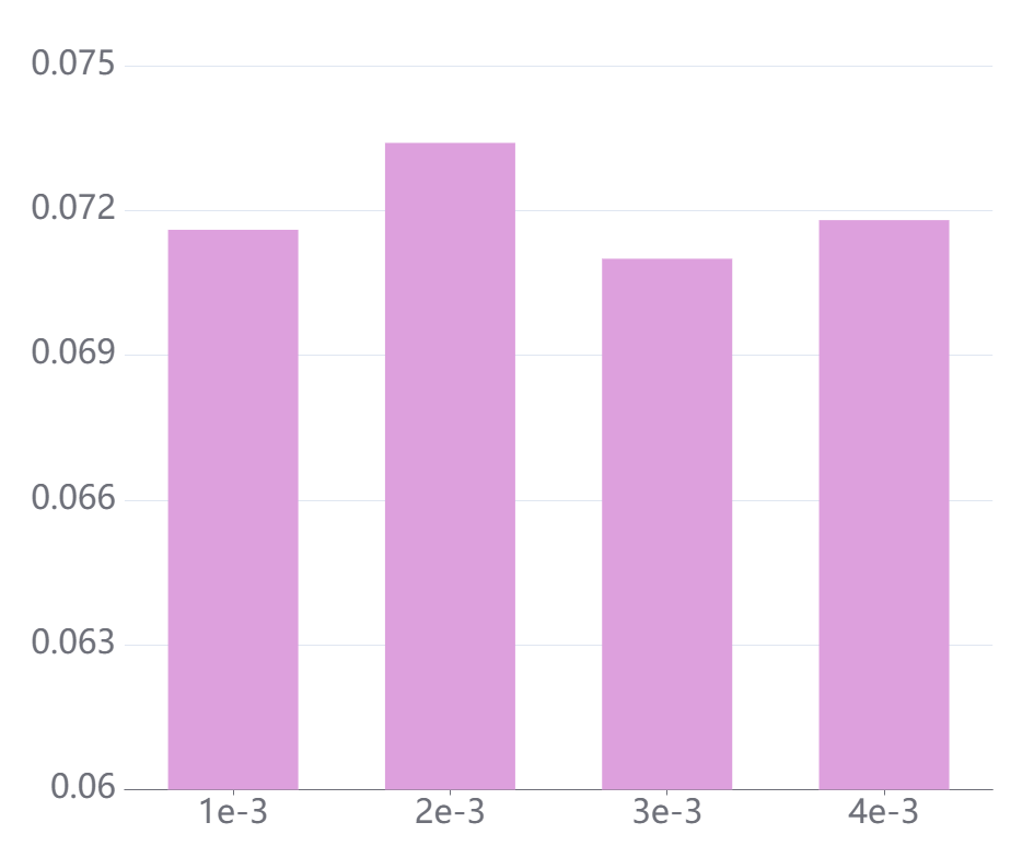
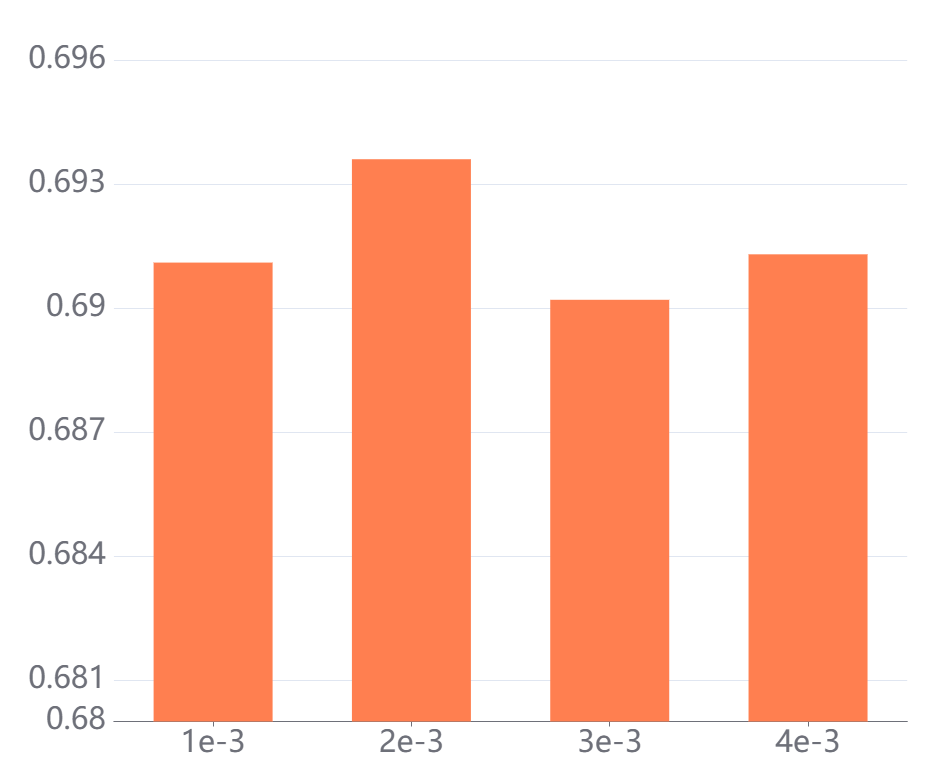
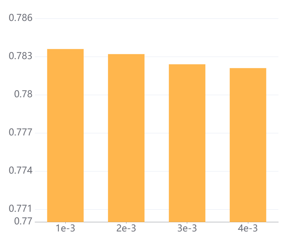
(d) The impact of pre training learning rate on results.

Figure 4: Experiments on parameter sensitivity on MIMIC-III dataset.

To explore the impact of specific parameters on the model, we conduct a series of parameter sensitivity experiments on the MIMIC-III dataset, focusing on four key parameters of the model. These experiments aim to study the effects of different parameter combinations on model performance and analyze the reasons for these changes in detail. The results are shown in Figure 4, where the X-axis represents different values of a parameter, and the Y-axis indicates the performance differences caused by varying parameter values.

First, we investigate the impact of different embedding dimensions on experimental performance. Figure 4(a) shows the performance at embedding dimensions of 32, 64, 128, and 256. When the embedding size is 128, the model’s accuracy significantly exceeds that of other parameter settings, while safety remains at the same level. Therefore, considering accuracy, safety, and time cost, we select 128 as the optimal embedding dimension for this experiment.

Next, since both molecular modalities use GNN networks as the basic encoder, we consider the number of GNN layers. The specific impact is shown in Figure 4(b). It is clear that a 4-layer network achieves better accuracy. Too many layers increase the model’s complexity and make it more prone to overfitting, leading to a larger gap between training and testing results. Too few layers slow down the model’s convergence speed, and the model’s performance fails to reach the desired effect. Thus, we choose 4 layers for the model.

Regarding the number of epochs and learning rate of the pre-training model, these are crucial for the performance of the pre-trained model. As shown in Figure 4(c) and Figure 4(d), too few epochs fail to adequately conduct contrastive learning for the dual molecular modalities, while too many epochs are meaningless and can even decrease performance. The pre-training learning rate also requires fine-tuning, and using an optimizer strategy to adjust the learning step size is recommended.

In practical model experiments, adjustments can be made based on the experimental environment and actual results. Different experimental environments may lead to slight variations.

6.5 Case Study

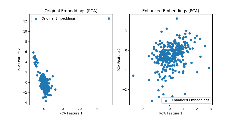
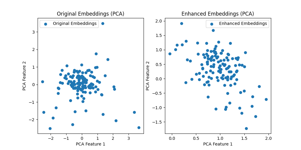
Figure 5: Low dimensional data distribution represented by molecular and substructure embeddings

To further elucidate the rationale behind our innovations, we conduct a case study using a sample from MIMIC-III. This specific instance demonstrates the existence of structural confusion issues and how they interfere with molecular representation and medication recommendation. It also highlights the importance of the interaction between molecular knowledge and individual patient visit representations in identifying key substructures for each visit.

Our model introduces 3D modality data, distinguishing molecules with very similar 2D structures and enhancing the differentiation between different molecules. This increases the information dimension of molecular representations, allowing similar molecular and substructural representations to better meet recommendation needs. After obtaining substructure representations, we use each patient’s visit representation to identify medication substructures strongly associated with the current patient’s condition. By using the patient’s latest representation as a calibration reference, we identify medication substructures relevant to the latest visit, thereby improving model accuracy and safety.

For example, the molecular structures of Atropine and Ipratropium are very similar, yet they have significant functional differences. Atropine is primarily used to treat conditions such as blurred vision and arrhythmia caused by various factors, while Ipratropium is mainly used to treat COPD (chronic obstructive pulmonary disease) and other respiratory diseases, administered via nebulization. By incorporating the 3D modality, we successfully distinguish between medications such as R01A and A03B, N07A, S01K, and recommend the correct medication to the user. As shown in Figure 5, we observe that the molecular embeddings generated by the original molecular encoder and the dual-modality encoder in low-dimensional display show a more uniform distribution, better distinguishing the roles and functions of different molecules.

7 Conclusion

This paper introduces our developed medication recommendation model, BiMoRec. By integrating dual-modality molecular representations, the model addresses the structural confusion problem and significantly enhances the distinction between molecules, achieving notable improvements in molecular recognition. Furthermore, through single interactions between molecular knowledge and patient representations, and by distilling substructures at both the visit level and the overall level using the patient’s latest visit representation, the model identifies truly useful substructures, thereby significantly improving accuracy and safety. We conduct a series of rigorous experiments on publicly available clinical datasets to demonstrate the validity of our approach.

Despite the significant advancements in the field of medication recommendation made by our research, certain limitations remain, potentially offering directions for future research. Currently, medication recommendation systems in our country hold substantial theoretical and scientific research value, as well as practical significance, with the potential to address major societal issues effectively. In actual medical systems, clinicians need AI-based diagnostic support and medication review systems. Therefore, we plan to continue our in-depth research in the fields of medication recommendation and medical large models, leveraging large models to enhance our ability to tackle complex problems and real-world scenarios based on the current model.

Declaration of Competing Interest

The authors declare that they have no known competing financial interests or personal relationships that could have appeared to influence the work reported in this paper.

References

- An et al. [2021] An, Y., Zhang, L., You, M., Tian, X., Jin, B., Wei, X., 2021. Mesin: Multilevel selective and interactive network for medication recommendation. Knowledge-Based Systems 233, 107534.
- Bougiatiotis et al. [2020] Bougiatiotis, K., Aisopos, F., Nentidis, A., Krithara, A., Paliouras, G., 2020. Drug-drug interaction prediction on a biomedical literature knowledge graph, in: Artificial Intelligence in Medicine: 18th International Conference on Artificial Intelligence in Medicine, AIME 2020, Minneapolis, MN, USA, August 25–28, 2020, Proceedings 18, Springer. pp. 122–132.
- Chen et al. [2023] Chen, Q., Li, X., Geng, K., Wang, M., 2023. Context-aware safe medication recommendations with molecular graph and ddi graph embedding, in: Proceedings of the AAAI Conference on Artificial Intelligence, pp. 7053–7060.
- Chen et al. [2020] Chen, T., Kornblith, S., Norouzi, M., Hinton, G., 2020. A simple framework for contrastive learning of visual representations. Cornell University - arXiv,Cornell University - arXiv .
- Chen and Wong [2020] Chen, T., Wong, R.C.W., 2020. Handling information loss of graph neural networks for session-based recommendation, in: Proceedings of the 26th ACM SIGKDD International Conference on Knowledge Discovery & Data Mining, pp. 1172–1180.
- Chiang et al. [2020] Chiang, W.H., Shen, L., Li, L., Ning, X., 2020. Drug-drug interaction prediction based on co-medication patterns and graph matching. International Journal of Computational Biology and Drug Design 13, 36–57.
- Choi et al. [2016] Choi, E., Bahadori, M.T., Sun, J., Kulas, J., Schuetz, A., Stewart, W., 2016. Retain: An interpretable predictive model for healthcare using reverse time attention mechanism. Advances in Neural Information Processing Systems 29.
- Dauji and Bhargava [2016] Dauji, S., Bhargava, K., 2016. Estimation of concrete characteristic strength from limited data by bootstrap. Journal of Asian Concrete Federation 2, 81–94.
- Hoffman et al. [2014] Hoffman, K.B., Dimbil, M., Erdman, C.B., Tatonetti, N.P., Overstreet, B.M., 2014. The weber effect and the united states food and drug administration’s adverse event reporting system (faers): analysis of sixty-two drugs approved from 2006 to 2010. Drug safety 37, 283–294.
- Jin et al. [2018] Jin, B., Yang, H., Sun, L., Liu, C., Qu, Y., Tong, J., 2018. A treatment engine by predicting next-period prescriptions, in: Proceedings of the 24th ACM SIGKDD International Conference on Knowledge Discovery & Data Mining, pp. 1608–1616.
- Jing et al. [2020] Jing, B., Eismann, S., Suriana, P., Townshend, R., Dror, R., 2020. Learning from protein structure with geometric vector perceptrons. Learning,Learning .
- Johnson et al. [2023] Johnson, A.E., Bulgarelli, L., Shen, L., Gayles, A., Shammout, A., Horng, S., Pollard, T.J., Hao, S., Moody, B., Gow, B., et al., 2023. Mimic-iv, a freely accessible electronic health record dataset. Scientific data 10, 1.
- Johnson et al. [2016] Johnson, A.E., Pollard, T.J., Shen, L., Lehman, L.w.H., Feng, M., Ghassemi, M., Moody, B., Szolovits, P., Anthony Celi, L., Mark, R.G., 2016. Mimic-iii, a freely accessible critical care database. Scientific data 3, 1–9.
- Le et al. [2018a] Le, H., Tran, T., Venkatesh, S., 2018a. Dual memory neural computer for asynchronous two-view sequential learning, in: Proceedings of the 24th ACM SIGKDD International Conference on Knowledge Discovery & Data Mining, pp. 1637–1645.
- Le et al. [2018b] Le, H., Tran, T., Venkatesh, S., 2018b. Dual memory neural computer for asynchronous two-view sequential learning, in: Proceedings of the 24th ACM SIGKDD International Conference on Knowledge Discovery & Data Mining, pp. 1637–1645.
- Li et al. [2023] Li, X., Liang, S., Hou, Y., Ma, T., 2023. Stratmed: Relevance stratification between biomedical entities for sparsity on medication recommendation. Knowledge-Based Systems , 111239.
- Lin et al. [2020] Lin, X., Quan, Z., Wang, Z.J., Ma, T., Zeng, X., 2020. Kgnn: Knowledge graph neural network for drug-drug interaction prediction., in: IJCAI, pp. 2739–2745.
- Liu et al. [2021] Liu, S., Wang, H., Liu, W., Lasenby, J., Guo, H., Tang, J., 2021. Pre-training molecular graph representation with 3d geometry. arXiv preprint arXiv:2110.07728 .
- Picheny et al. [2010] Picheny, V., Kim, N.H., Haftka, R.T., 2010. Application of bootstrap method in conservative estimation of reliability with limited samples. Structural and Multidisciplinary Optimization 41, 205–217.
- Quadrana et al. [2017] Quadrana, M., Karatzoglou, A., Hidasi, B., Cremonesi, P., 2017. Personalizing session-based recommendations with hierarchical recurrent neural networks, in: Proceedings of the Eleventh ACM Conference on Recommender Systems, pp. 130–137.
- Read et al. [2011] Read, J., Pfahringer, B., Holmes, G., Frank, E., 2011. Classifier chains for multi-label classification. Machine learning 85, 333–359.
- Schütt et al. [2017] Schütt, K., Kindermans, P.J., Sauceda, H., Chmiela, S., Tkatchenko, A., Müller, K.R., 2017. Schnet: A continuous-filter convolutional neural network for modeling quantum interactions. Neural Information Processing Systems,Neural Information Processing Systems .
- Shang et al. [2019] Shang, J., Xiao, C., Ma, T., Li, H., Sun, J., 2019. Gamenet: Graph augmented memory networks for recommending medication combination, in: Proceedings of the AAAI Conference on Artificial Intelligence, pp. 1126–1133.
- Stark et al. [2021] Stark, H., Beaini, D., Corso, G., Tossou, P., Dallago, C., Günnemann, S., Liò, P., 2021. 3d infomax improves gnns for molecular property prediction. arXiv: Learning,arXiv: Learning .
- Thomas et al. [2018] Thomas, N., Smidt, T., Kearnes, S., Yang, L., Li, L., Kohlhoff, K., Riley, P., 2018. Tensor field networks: Rotation- and translation-equivariant neural networks for 3d point clouds. arXiv: Learning,arXiv: Learning .
- Wang et al. [2022a] Wang, L., Liu, Y., Lin, Y., Liu, H., Ji, S., 2022a. Comenet: Towards complete and efficient message passing for 3d molecular graphs. Advances in Neural Information Processing Systems 35, 650–664.
- Wang et al. [2017] Wang, M., Liu, M., Liu, J., Wang, S., Long, G., Qian, B., 2017. Safe medicine recommendation via medical knowledge graph embedding. arxiv. Information Retrieval .
- Wang et al. [2022b] Wang, Z., Liang, Y., Liu, Z., 2022b. Ffbdnet: Feature fusion and bipartite decision networks for recommending medication combination, in: Joint European Conference on Machine Learning and Knowledge Discovery in Databases, Springer. pp. 419–436.
- Wu et al. [2022] Wu, R., Qiu, Z., Jiang, J., Qi, G., Wu, X., 2022. Conditional generation net for medication recommendation, in: Proceedings of the ACM Web Conference 2022, pp. 935–945.
- Xu et al. [2018] Xu, K., Hu, W., Leskovec, J., Jegelka, S., 2018. How powerful are graph neural networks? arXiv preprint arXiv:1810.00826 .
- Yang et al. [2021a] Yang, C., Xiao, C., Glass, L., Sun, J., 2021a. Change matters: Medication change prediction with recurrent residual networks, in: Proceedings of the Thirtieth International Joint Conference on Artificial Intelligence 2021, pp. 3728–3734.
- Yang et al. [2021b] Yang, C., Xiao, C., Ma, F., Glass, L., Sun, J., 2021b. Safedrug: Dual molecular graph encoders for safe drug recommendations, in: Proceedings of the Thirtieth International Joint Conference on Artificial Intelligence, IJCAI 2021, pp. 3735–3741.
- Yang et al. [2023] Yang, N., Zeng, K., Wu, Q., Yan, J., 2023. Molerec: Combinatorial drug recommendation with substructure-aware molecular representation learning, in: Proceedings of the ACM Web Conference 2023, pp. 4075–4085.
- Zhang et al. [2017] Zhang, Y., Chen, R., Tang, J., Stewart, W.F., Sun, J., 2017. Leap: learning to prescribe effective and safe treatment combinations for multimorbidity, in: Proceedings of the 23rd ACM SIGKDD International Conference on Knowledge Discovery and Data Mining, pp. 1315–1324.
- Zheng et al. [2021a] Zheng, Z., Wang, C., Xu, T., Shen, D., Qin, P., Huai, B., Liu, T., Chen, E., 2021a. Drug package recommendation via interaction-aware graph induction, in: Proceedings of the Web Conference 2021, pp. 1284–1295.
- Zheng et al. [2021b] Zheng, Z., Wang, C., Xu, T., Shen, D., Qin, P., Huai, B., Liu, T., Chen, E., 2021b. Drug package recommendation via interaction-aware graph induction, in: Proceedings of the Web Conference 2021, pp. 1284–1295.
- Zheng et al. [2023] Zheng, Z., Wang, C., Xu, T., Shen, D., Qin, P., Zhao, X., Huai, B., Wu, X., Chen, E., 2023. Interaction-aware drug package recommendation via policy gradient. ACM Transactions on Information Systems 41, 1–32.
- Zhu et al. [2022] Zhu, J., Xia, Y., Wu, L., Xie, S., Qin, T., Zhou, W., Li, H., Liu, T.Y., 2022. Unified 2d and 3d pre-training of molecular representations, in: Proceedings of the 28th ACM SIGKDD conference on knowledge discovery and data mining, pp. 2626–2636.