Mixed finite element methods for fourth order obstacle problems in linearised elasticity
Paolo Piersanti
School of Science and Engineering, The Chinese University of Hong Kong (Shenzhen), 2001 Longxiang Blvd., Longgang District, Shenzhen, China
ppiersanti@cuhk.edu.cn and Tianyu Sun
Department of Mathematics and Institute for Scientific Computing and Applied Mathematics, Indiana University Bloomington, 729 East Third Street, Bloomington, Indiana, USA
ts19@iu.edu
Abstract.
This paper is devoted to the study of a novel mixed Finite Element Method for approximating the solutions of fourth order variational problems subjected to a constraint.
The first problem we consider consists in establishing the convergence of the error of the numerical approximation of the solution of a biharmonic obstacle problem. The contents of this section are meant to generalise the approach originally proposed by Ciarlet & Raviart, and then complemented by Ciarlet & Glowinski.
The second problem we consider amounts to studying a two-dimensional variational problem for linearly elastic shallow shells subjected to remaining confined in a prescribed half-space. We first study the case where the parametrisation of the middle surface for the linearly elastic shallow shell under consideration has non-zero curvature, and we observe that the numerical approximation of this model via a mixed Finite Element Method based on conforming elements requires the implementation of the additional constraint according to which the gradient matrix of the dual variable has to be symmetric. However, differently from the biharmonic obstacle problem previously studied, we show that the numerical implementation of this result cannot be implemented by solely resorting to Courant triangles.
Finally, we show that if the middle surface of the linearly elastic shallow shell under consideration is flat, the symmetry constraint required for formulating the constrained mixed variational problem announced in the second part of the paper is not required, and the solution can thus be approximated by solely resorting to Courant triangles.
The theoretical results we derived are complemented by a series of numerical experiments.
Keywords. Obstacle problems Variational Inequalities Elasticity Theory Penalty Method Finite Element Method
MSC 2010. 35J86, 47H07, 65M60, 74B05.
1. Introduction
Fourth order variational problems appear in a manifold of applications like, for instance, elasticity [8, 29, 37], Fluid-Structure-Interaction [27] and phase transition problems [39, 41]. It is possible that the solutions of these models might have to satisfy certain constraints of analytical, physical or geometrical nature, thus rendering the problems under consideration obstacle problems.
In this paper, we are interested in the numerical approximation of obstacle problems in linearised elasticity modelled by means of fourth order differential operators. In particular, we are interested in the numerical approximation of the solutions of two-dimensional models describing the deflection of thin films subjected to a certain geometrical constraint. In general, the models we will be considering are recovered upon completion of a rigorous asymptotic analysis departing from the standard energy of three-dimensional linearised elasticity. The mathematical justification of obstacle problems in linearised elasticity via a rigorous asymptotic analysis was initiated in [35, 36] in the case where the elastic structure under consideration is a linearly elastic shallow shell. However, the constraint considered in the latter two papers was only affecting the transverse component of the displacement field. The mathematical justification of obstacle problems for linearly elastic shells and their numerical analysis was then continued in the papers [20, 21, 24, 25, 40, 43, 44, 45, 46, 49, 51, 52].
Differently from the existing literature about the approximation of the solution of obstacle problems governed by fourth order operators, which is mainly based on Morley Finite Elements, Hsieh-Clough-Tocher Finite Elements, and Enriching operators [3, 7, 47], the method we propose in this paper is meant to work with Courant triangles. The convergence of the method we are going to propose will be, in general, not faster than the methods based on more complex Finite Elements. However, its implementation will be feasible in those libraries which do not come equipped with Finite Elements for fourth order differential operators. The effectiveness of the methods based on Enriching Operators seem, instead, to be limited to scalar fourth order obstacle problems [3] and vector-valued fourth order obstacle problems in elasticity where the constraint hinges on the sole transverse component of the solution [47].
The new method we are going to propose in this paper is meant to overcome the limitations arising in the methods based on Enriching Operators, and will allow us to perform the numerical study of obstacle problems in elasticity whose solutions are vector fields, and whose constraint hinges at once on all the components of the solution. The latter situation contemplate the cases where an elastic body has to remain confined in a prescribed half-space or in the convex part of the three-dimensional Euclidean space identified by a finite number of intersecting planes.
The paper is divided into six sections, including this one, in the remainder of which the basic notation will be recalled.
In section 2, we present a new Finite Element Method for the prototypical biharmonic obstacle problem. The new method we are going to discuss also works as an alternative approach to the discretisation of the biharmonic equation proposed first by Ciarlet & Raviart [22], and then complemented by Ciarlet & Glowinski [16]. The mixed Finite Element Method proposed in [22] discretises the solution of the biharmonic equation by introducing a finite-dimensional space which is in general not a subspace of the vector space where the mixed formulation is posed and, moreover, the primal variable and the dual variable appearing in the mixed formulation are, in general, not independent of each other (cf., e.g., the remark after Theorem 7.1.4 of [9]). Besides, the actual computation of the pair solving the discrete mixed problem is carried out by means of the Uzawa Method (cf., e.g., [9] for a detailed description).
The main advantages in the method we propose are, first, that the finite-dimensional space where we discretise the mixed variational formulation for the obstacle problem for the biharmonic operator is a subspace of the space where the mixed obstacle problem is posed and, second, that the computation of the solution is carried out by standard Newton’s method, as the primal and dual variables are now independent of each other.
The method we are going to present contemplates two layers of relaxation of the main problem: one layer of relaxation for the implementation of the geometrical constraint, and another layer of relaxation for the dual variable so as to reduce the problem to a second order variational problem. In order to be able to establish the existence and uniqueness of solutions for this penalised mixed formulation, we introduce a harmonic corrector. We also show that, under suitable assumptions on the given data, the solution of the penalised mixed formulation converges to the solution of the original fourth order obstacle problem as the penalty parameter approaches zero.
Finally, we discretise the penalised mixed formulation by means of Courant triangles, and we show that the error converges to zero as the mesh size approaches zero.
We anticipate that, for the sake of readability of this article, we shall not be proving any results concerning the augmentation of regularity for the solutions, but we shall just redirect the reader to the related bibliographical references.
In section 3, we present numerical results corroborating the theoretical results obtained in section 2.
In section 4, we consider a fourth-order obstacle problem for linearly elastic shallow shells constrained to remain confined in a prescribed half-space. We observe that the mixed formulation proposed in [22] that related the dual variable to the Laplacian of the primal variable cannot be exploited in the framework of the problem we are discussing in section 4 because of the presence of mixed second order derivatives in the variational formulation. Following the steps in section 2, we introduce the corresponding penalised mixed formulation of the problem under consideration. Differently from the scalar case, the competitors to the role of solution for the penalised mixed formulation will be those for which the gradient matrix of the dual variable is symmetric. In order to establish the existence and uniqueness of solutions for one such penalised mixed formulation, we need a new preparatory inequality of Korn’s type in mixed coordinates. The proof of this preparatory result hinges on the assumption that the domain on which the problem is posed is simply connected, so as to apply the weak Poincaré lemma.
The reason why we cannot avoid the aforementioned symmetry constraint for the gradient matrix of the dual variable is due to the fact that, differently from the linearly elastic shells thoroughly discussed in [12], there is no rigidity theorem available for two-dimensional models for linearly elastic shallow shells.
We are thus in a position to establish the existence and uniqueness of solutions for the penalised mixed formulation under an essential assumption on the given forcing term.
Finally, we proceed with the discretisation of the penalised mixed formulation. In order to handle the constraint according to which the gradient of the dual variable is a symmetric matrix, we exploit the Functional Analysis theory of incompressible Stokes and Navier-Stokes equations [28, 50].
We then show that the error converges to zero as the mesh size approaches zero. The fact that we have to resort to the theory of incompressible Stokes and Navier-Stokes equations [28, 50] compels us to resort to Finite Elements for discretising the stream functions like, for instance, the Hsieh-Clough-Tocher triangles. This shows that we cannot avoid resorting to Finite Elements of more complex nature for approximating the solution of the mixed obstacle problem for linearly elastic shallow shells with middle surface having non-zero curvature we are considering.
In section 5, we consider the fourth order obstacle problem for linearly elastic shallow shells presented in section 4, and we assume that the middle surface of the linearly elastic shallow shell under consideration is flat. We show that, in the case of this special geometry, rigidity is regained, and the constraint according to which the gradient matrix of the dual variable has to be symmetric can thus be dropped. As a result, the discretisation of the penalised mixed formulation can be performed by standard Courant triangles.
In section 6, we present numerical results for approximating the solution of the obstacle problem for linearly elastic shallow shells considered in sections 4 and 5 using two different Finite Element Analysis libraries.
For an overview about the classical notions of differential geometry used in this paper see, e.g., [12] or [13] while, for an overview about the classical notions of functional analysis used in this paper see [14].
Latin indices, except , take their values in the set while Greek indices, except , and , take their values in the set . The Einstein summation convention is systematically used in conjunction with these two rules unless differently specified.
The notation indicates the three-dimensional Euclidean space.
We denote by the standard Kronecker symbol.
Given an open subset of , where , we denote the usual Lebesgue and Sobolev spaces by , , , , or . Given a set , the Cartesian product is denoted by , while the Cartesian product is denoted by . In what follows, the abbreviations “a.a.” and “a.e.” stand for almost all and almost everywhere, respectively. Spaces of symmetric tensors are denoted in blackboard bold letters like for instance .
In order to favour the readability of this article, we resort to the notation to denoted the positive constant of the Poincaré-Friedrichs inequality and its variants.
In all what follows, we denote by a Lipschitz domain, namely a non-empty bounded open connected subset of with Lipschitz continuous boundary and such that is all on the same side of (cf., e.g., Section 1.18 in [14]). Let denote a generic point in and let and .
In what follows denotes the outer unit normal vector field to the boundary and denotes the outer unit normal derivative operator along .
2. A prototypical example of fourth order obstacle problem. The biharmonic model
The first problem we study is a prototypical variational problem modelling the deflection of a linearly elastic plate. Let the function be given.
The free energy functional associated with the model under consideration is denoted by , and is defined by:
Let us recall that the bilinear form defined by
is continuous, symmetric, and -elliptic thanks to the Poincaré-Friedrichs inequality for fourth order operators (cf., e.g., Theorem 6.8-4 in [14]). Also recall that the linear form defined by
is continuous.
Let be a given function such that and such that , for all . The given function represents the obstacle that the deformed plate does not have to cross. In order to determine the equilibrium configuration of a plate subjected not to cross the given function , we must restrict our search for solutions to functions such that , for all , and we note that the constraint has to hold everywhere up the boundary since in light of the Rellich-Kondrašov Theorem (cf., e.g., Theorem 6.6-3 in [14]).
The latter considerations imply that we need to restrict our search for solutions to the functions in the following non-empty, closed and convex subset of , denoted and defined by:
It is thus classical to establish (cf., e.g., Section 6.8 in [14]) that the following minimisation problem
(1)
admits a unique solution . In addition to this, following a strategy similar to the one implemented in [45, 47], it can be shown that the solution of the minimisation problem (1) satisfies .
Let us recall that a regularity of class is not in general achievable in light of the counterexample contrived by Caffarelli and his collaborators for fourth order obstacle problems [5, 6].
Since is a Lipschitz domain and since any satisfies , we have that for fixed (no summation) indices , an application of Green’s formula (cf., e.g., Theorem 1.18-2 in [14]) gives:
The minimisation problem (1) can thus be equivalently formulated in terms of the following variational inequalities.
Problem .
Find satisfying:
for all .
The numerical approximation of the solution for Problem was recently studied in [3], where the authors exploited the properties of Enriching Operators to derive the error estimates for the difference between the exact solution and a suitable Finite Element approximation. The strategy in [3] made use of Morley’s triangles to derive the error estimates. The apparent drawback in the implementation of this strategy lies in the fact that Morely’s triangles are not implemented in a number of Finite Element libraries.
A generalisation of the strategy presented in the paper [3] was recently proposed in [47], where we studied a numerical method - based on Enriching Operators - for approximating the solution of an obstacle problem for linearly elastic shallow shells. Note, however, that the proofs in [47] only work if the constraint is imposed on the sole transverse component of the solution of the problem under consideration, which represents the displacement of the linearly elastic shallow shell involved in the analysis. Apparently, the method of Enriching Operators does not work for treating the numerical convergence in the case of more general constraints, like for instance, when the deformed reference configuration is required to remain confined in the convex part of the Euclidean space identified by the intersection of two planar obstacles.
The alternative strategy we propose in this section to numerically approximate the solution of Problem will serve to devise a new numerical method for approximating the displacement of linearly elastic shallow shells subjected to remaining confined in the convex portion of the Euclidean space identified by a finite number of planes in a way that the constraint will affect at once all the components of the displacement field, thus generalising the result established in [47]. The novelty in the strategy we are proposing consists in approximating the solution of Problem by means of Courant triangles (cf., e.g., Section 2.2 in [9]).
The fist step to achieve this goal consists in penalising Problem , by incorporating the constraint in the variational formulation of the problem. The latter relaxation will allow us to replace the variational inequalities appearing in problem by a set of non-linear variational equations posed over the entire space . In what follows, we denote by a positive penalty parameter which is meant to approach zero and the mapping defined by , a.e. in is the negative part of the function .
The monotonicity properties of the negative part of a function are classical (cf., e.g., [48]). We are now in position to state the penalised version of Problem .
Problem .
Find satisfying:
for all .
The existence and uniqueness of solutions for Problem are classical, as the strong monotonicity of the left-hand side of the previous variational equations allows us to apply the Minty-Browder Theorem (cf., e.g., Theorem 9.14-1 in [14]). Next, we establish that the sequence of solutions of Problem strongly converges in to the solution of Problem .
Theorem 2.1.
Let be the unique solution of Problem . For each , denote by the unique solution of Problem . Then, the sequence is such that
Proof.
Specialising in the variational equations of Problem , we obtain that the following energy estimates hold as a result of Theorem 6.8-4 in [14] and Hölder’s inequality (cf., e.g., [4]):
where denotes the constant of the Poincaré-Friedrichs inequality for fourth order differential operators (cf., e.g., Theorem 6.8-4 of [14]), which solely depends on the geometry of the Lipschitz domain .
As a result, we obtain that , thus showing that is bounded in independently of . It is straightforward to see that the latter boundedness gives:
Therefore, up to passing to subsequences, we have that
(2)
An application of Theorem 9.13-2 of [14] immediately gives that a.e. in or, equivalently, that in , being and . Hence, we have that .
Testing the variational equations of Problem on , where is arbitrary, gives:
(3)
Taking the as in (3) gives that the weak limit of the sequence satisfies:
The arbitrariness of let us straightforwardly infer that is the solution of Problem .
To show that the weak convergence is actually strong, we test the variational equations in Problem on . We obtain that an application of Theorem 6.8-4 of [14] gives:
(4)
Exploiting the weak convergence in (2), we obtain that letting in (4) gives that:
thus showing the sought strong convergence and completing the proof.
∎
Combining the techniques presented in [40] to handle the penalty term with the techniques presented in [45, 43], we obtain that . Moreover, since , we have that the constraint is inactive in a neighbourhood of the boundary. Therefore, applying the standard augmentation-of-regularity techniques for fourth order variational problems (cf., e.g., [38]), we obtain that
(5)
The augmentation-of-regularity result in (5) will play a crucial role for establishing the convergence of the mixed Finite Element Method we are going to discuss next. We immediately observe that the regularity of does not consent, a priori, to perform its approximation by means of Courant triangles. Potential elements to approximate could be Hsieh-Clough-Tocher triangles, Argyris triangles and Morely’s triangles, to cite some (viz., e.g., [9]).
However, as we mentioned beforehand, these Finite Elements are not implemented in a number of Finite Element packages. The method we are going to present next allows us to overcome these difficulties, by allowing us to discretise the penalised solution for the original variational Problem .
We introduce a further layer of penalisation, by introducing a mixed formulation for Problem . In order to have a sound formulation, the following assumption on the given forcing term must be made: There exists a vector field such that a.e. in . Note that this assumption is reasonable in light of Bogovskii’s Theorem (cf., e.g., Theorem 6.14-1 in [14] and the commentary part at the end of Section 7 of [9]).
For a treatment of the spaces see Section 6.13 in [14], for instance.
The corresponding mixed formulation associated with Problem , which we shall be referring to as Problem , can thus be stated.
Problem .
Find satisfying:
for all .
Clearly, Problem admits a unique solution as re-writing of Problem . Note that since and .
The next layer of approximation consists in formulating a mixed variational problem that takes into account the penalty term introduced in Problem as well as an additional penalty term to steer the solutions towards states where the dual variable is as close as possible to the gradient of the primal variable. The weak formulation for one such variational problem takes the following form.
Problem .
Find satisfying:
for all .
We observe that Problem is the most relaxed formulation for the original Problem , as solutions are sought in a linear space, and the constraints associated with the obstacle and with the dual variable are implemented directly in the model. The harmonic corrector appearing in the first term will play a fundamental role in establishing the existence and uniqueness of solutions for Problem , as it is shown in the next theorem.
Theorem 2.2.
For each , Problem admits a unique solution . Besides, we have that the following convergences hold
where is the unique solution of Problem .
Proof.
To begin with, we observe that the left-hand side of the variational equations in Problem is made of the sum of bilinear forms which are symmetric and continuous, and of a monotone operator. The right-hand side, instead, is a linear and continuous form.
In order to assert the existence and uniqueness of solutions, we need to establish the coerciveness of the left-hand side so as to apply the Minty-Browder Theorem (cf., e.g., Theorem 9.14-1 in [14]).
Specialising in the variational equations of Problem , we obtain that an application of the classical Poincaré-Friedrichs inequality (cf., e.g., Theorem 6.5-2 of [14]) gives:
The latter estimate in turn implies that , so that it results that the sequence is bounded in independently of .
As a result, we obtain that
(6)
Therefore, we obtain that an application of the triangle inequality and of the second estimate in (6) give:
which in turn implies that the sequence is bounded in independently of . Another application of the classical Poincaré-Friedrichs inequality (cf., e.g., Theorem 6.5-2 in [14]) gives that:
which in turn implies that the sequence is bounded in independently of . Therefore, up to passing to subsequences, we obtain that:
(7)
In particular, the fact that and implies that , being a Lipschitz domain. Hence, we have that . Let us now fix an arbitrary , and let us test the variational equations in Problem on . We obtain that:
(8)
Upon passing to the as , the convergence process (7) yields:
(9)
Since , we obtain that:
Given the arbitrariness of , we infer that is the solution of Problem .
∎
In regard to the proof of Theorem 2.2, we observe that the assumption on the applied body force plays a crucial role in establishing the convergences in (7). Indeed, without this regularity assumption on , the right-hand side of the non-linear variational equations in Problem should be expressed in terms of the primal variable and, therefore, the boundedness of the sequence in independently of could not be inferred by the energy estimates.
The remainder of this section is devoted to the discretisation of the solution of Problem via the Finite Element Method. In what follows, for each , we denote by an affine regular triangulation of the Lipschitz domain (cf., e.g., [9]) made of Courant triangles. We denote by the finite-dimensional subspace of associated with one such triangulation . The discretisation of Problem can thus be formulated as follows.
Problem .
Find satisfying:
for all .
It is straightforward to observe that, akin to its continuum counterpart, Problem admits a unique solution . In the next theorem we are going to show that the solution of Problem converges, in some suitable sense, to the solution of Problem as .
Theorem 2.3.
Let be the unique solution of Problem , and let be the unique solution of Problem . Then, there exists a constant independent of and such that:
Proof.
In what follows, we denote by and the standard interpolation operators in and , respectively (cf., e.g., [9]).
Since and since , we are in a position to apply Theorem 3.2.1 in [9] so as to infer that:
(10)
for some independent of and .
Thanks to the fact that the forcing terms in the variational equations of Problem and Problem coincide, we have that an application of the classical Poincaré-Friedrichs inequality, Theorem 6.8-4 of [14], and Young’s inequality (cf., e.g., [53]) gives:
By the standard augmentation-of-regularity argument and the fact that the constraint is inactive near the boundary, we obtain that the semi-norms on the right-hand side of (10) are both of order .
An application of (10) thus yields:
where in the last inequality is the constant associated with the augmentation-of-regularity argument (cf., e.g., [42]) and depends on and the scaled forcing term only.
A rearrangement of the latter gives:
The proof is thus complete by letting .
∎
As a remark, if we specialise with it results, thanks to an application of Theorem 2.2 and Theorem 2.3, that the solution of Problem converges to the solution of Problem as .
We note in passing that the techniques presented in Theorem 7.1.6 of [9] for discretising the obstacle-free biharmonic problem hinge on a discretisation performed via conforming Finite Elements for fourth-order problems, whereas our technique only exploits Courant triangles. Not only the technique we developed requires less regularity for the solution, but - differently from the one in [15] - it can be implemented in Finite Element Analysis packages that do not come with Finite Elements for fourth order problems and with Enriched Finite Elements [2]. The crucial step for achieving this result is the presence of the harmonic corrector in the formulation of the penalised problem as well as the regularity assumption of the given forcing term.
We also observe that the method we presented could be applied for discretising the solution of the biharmonic equation, as an alternative to the method originally proposed by Ciarlet & Raviart [22], and then complemented by Ciarlet & Glowinski [16]. The differences between these methods and the method we are here proposing are, first, that the method discussed in [22] exploits a finite-dimensional space that is not a subspace of the space where the mixed formulation where the problem is defined, whereas our method discretises the mixed formulation over a finite-dimensional space of the space where the mixed formulation is posed and, second, the solution of the mixed formulation proposed in [22] is to be approximated via Uzawa’s method since the primal and dual variables do not vary independently, whereas in the mixed method we proposed the primal and dual variables vary independently.
3. Numerical experiments for the biharmonic obstacle problem
In this last section of the paper, we implement numerical simulations aiming to validate the theoretical results presented in section 2.
Consider as a domain a circle of radius , and denote one such domain by :
We constrain solution of Problem to remain confined above the function defined by:
The forcing term entering the first two batches of experiments is given by:
The numerical simulations are performed by means of the software FEniCS [34] and the visualization is performed by means of the software ParaView [1].
The plots were created by means of the matplotlib libraries from a Python 3.9.8 installation.
The first batch of numerical experiments is meant to validate the claim of Theorem 2.2. After fixing the mesh size , we let tend to zero in Problem . Let and be two solutions of Problem , where and .
The solution of Problem is discretised by Courant triangles (cf., e.g., [9]) and homogeneous Dirichlet boundary conditions are imposed for all the components.
At each iteration, Problem is solved by Newton’s method. The algorithm stops when the error is smaller than .
Error
1.5e-09
4.0e-07
7.5e-10
2.0e-07
3.7e-10
9.9e-08
1.8e-10
5.0e-08
9.3e-11
2.5e-08
4.6e-11
1.2e-08
2.3e-11
3.9e-09
(a)
(b)Error convergence as for . Original figure.
Error
3.7e-10
3.8e-07
1.9e-10
1.9e-07
9.3e-11
9.4e-08
4.6e-11
4.7e-08
2.3e-11
2.4e-08
1.2e-11
1.2e-08
5.8e-12
5.9e-09
(a)
(b)Error convergence as for . Original figure.
Error
9.3e-11
3.8e-07
4.7e-11
1.9e-07
2.3e-11
9.4e-08
1.2e-11
4.7e-08
5.8e-12
2.4e-08
2.9e-12
1.2e-08
1.5e-12
5.9e-09
(a)
(b)Error convergence as for . Original figure.
Error
2.3e-11
3.7e-07
1.2e-11
1.9e-07
5.8e-12
9.3e-08
2.9e-12
4.6e-08
1.5e-12
2.3e-08
7.3e-13
1.2e-08
3.6e-13
5.8e-09
(a)
(b)Error convergence as for . Original figure.
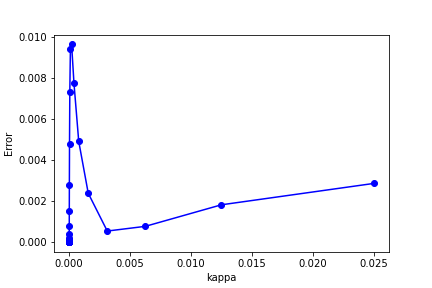
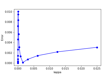
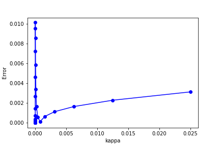
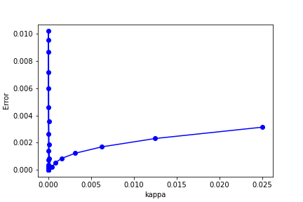
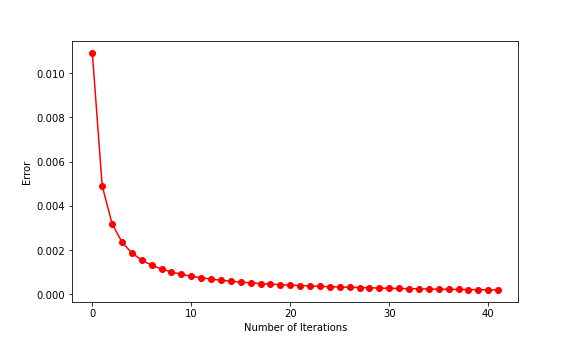
Figure 4. Given , the first component of the solution of Problem converges with respect to the standard norm of as .
From the data patterns in Figure 4 we observe that, for a given mesh size , the solution of Problem converges as . This is coherent with the conclusion of Theorem 2.2.
The second batch of numerical experiments is meant to validate the claim of Theorem 2.3.
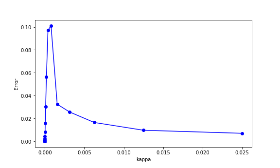
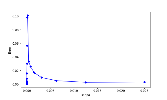
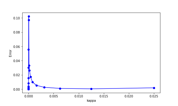
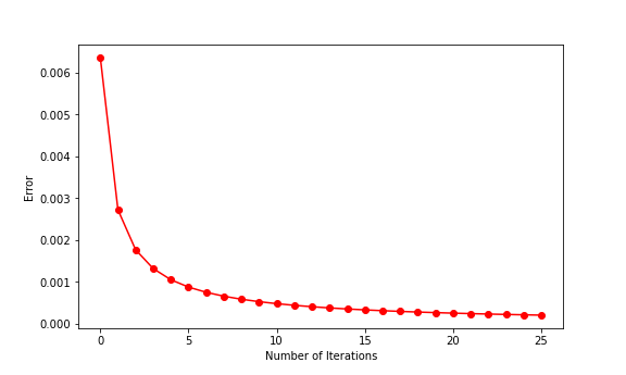
We show that, for a fixed as in Theorem 2.3, the error residual tends to zero as .
The algorithm stops when the error residual of the Cauchy sequence is smaller than .
Once again, each component of the solution of Problem is discretised by Lagrange triangles (cf., e.g., [9]) and homogeneous Dirichlet boundary conditions are imposed for all the components and, at each iteration, Problem is solved by Newton’s method.
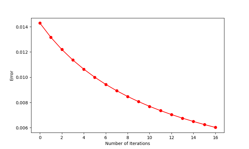
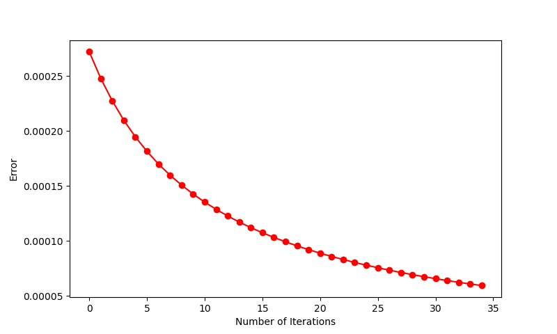
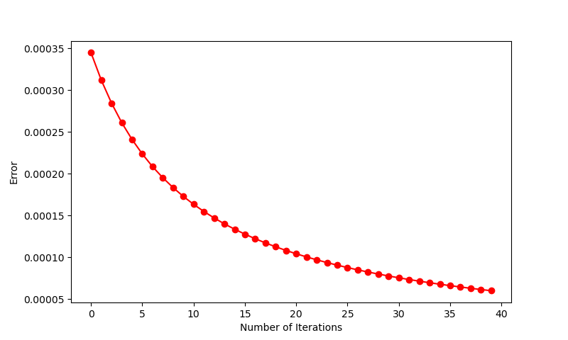
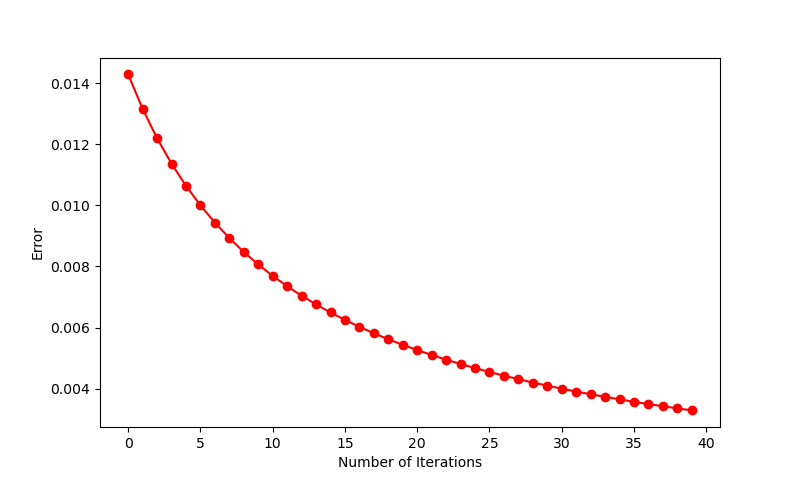
The results of these experiments are reported in Figure 6 below.
(a)For the algorithm stops after 16 iterations
(b)For the algorithm stops after 34 iterations
(a)For the algorithm stops after 39 iterations
(b)For the algorithm stops after 39 iterations
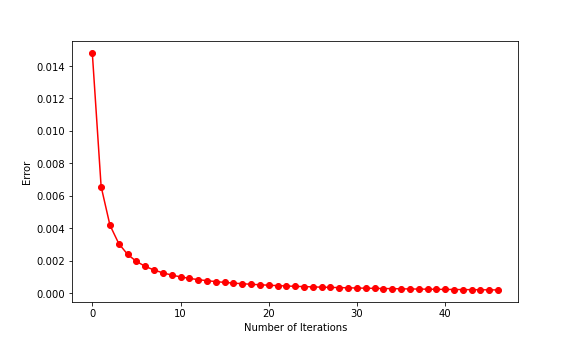
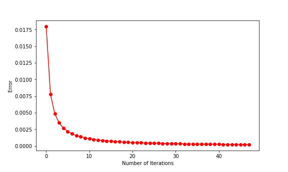
Figure 6. Given as in Theorem 2.2, the error converges to zero as . As increases, the number of iterations needed to meet the stopping criterion of the Cauchy sequence increases.
The third batch of numerical experiments validates the genuineness of the model from the qualitative point of view.
We observe that the presented data exhibits the pattern that, for a fixed and a fixed , the contact area increases as the applied body force intensity increases.
For the third batch of experiments, the applied body force density entering the model is given by
where is a non-negative integer.
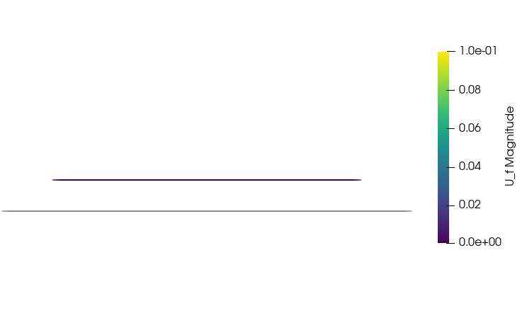
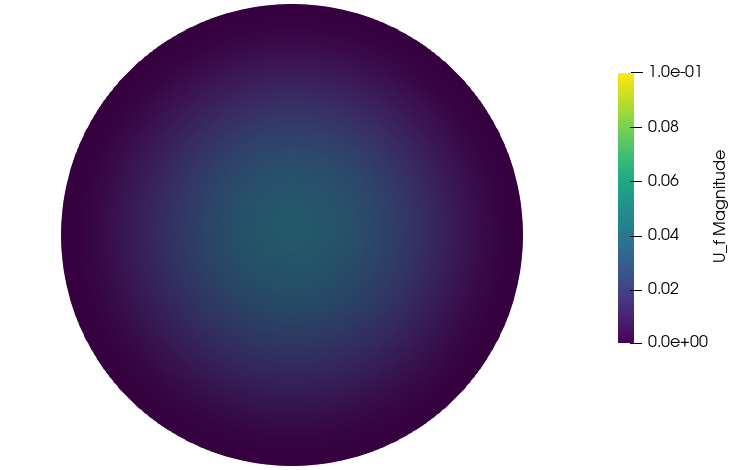
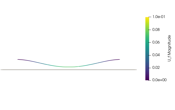
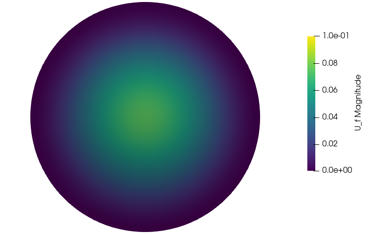
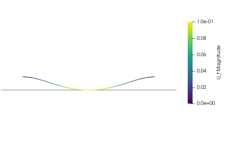
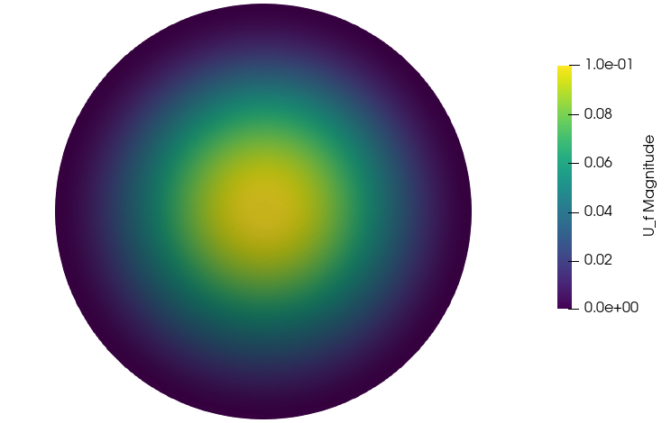
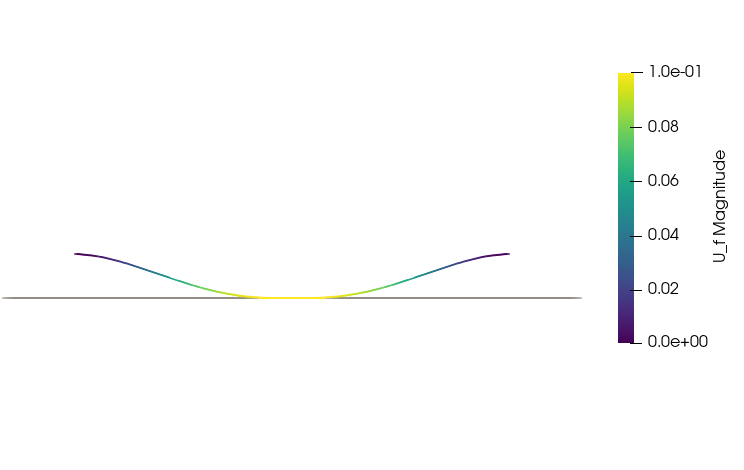
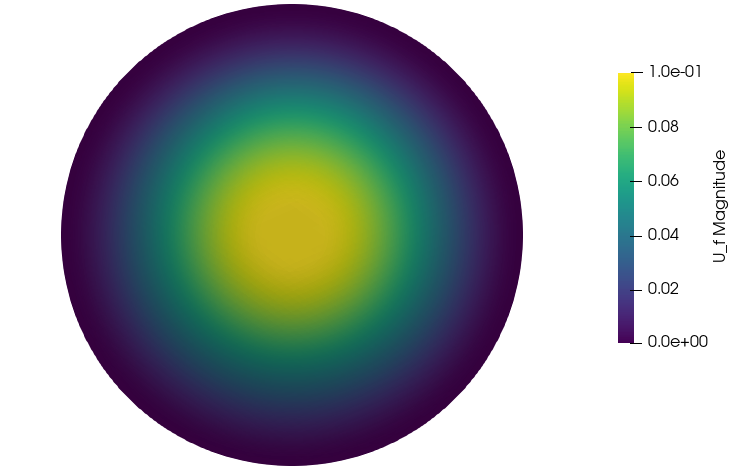
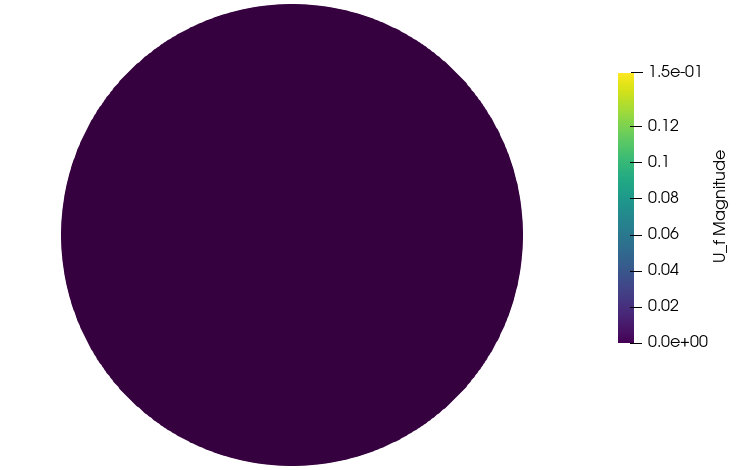
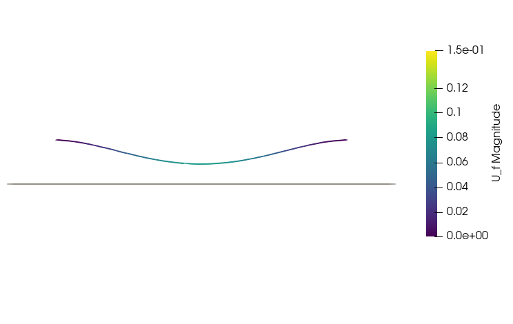
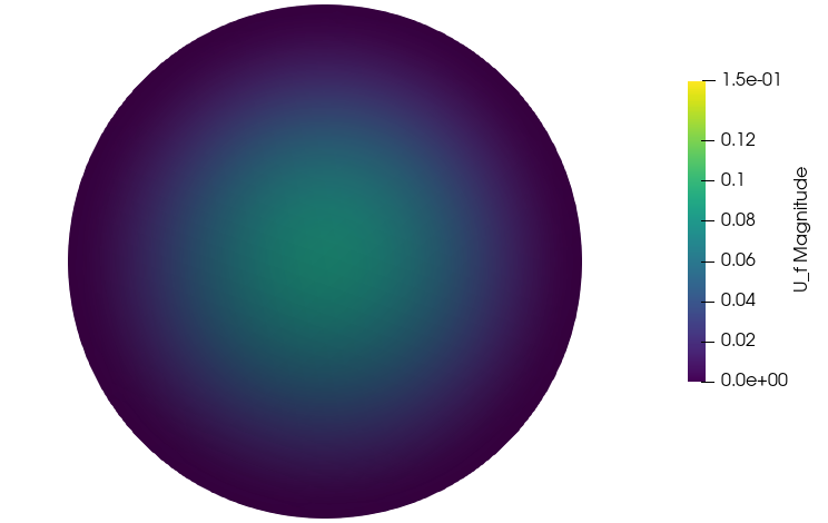
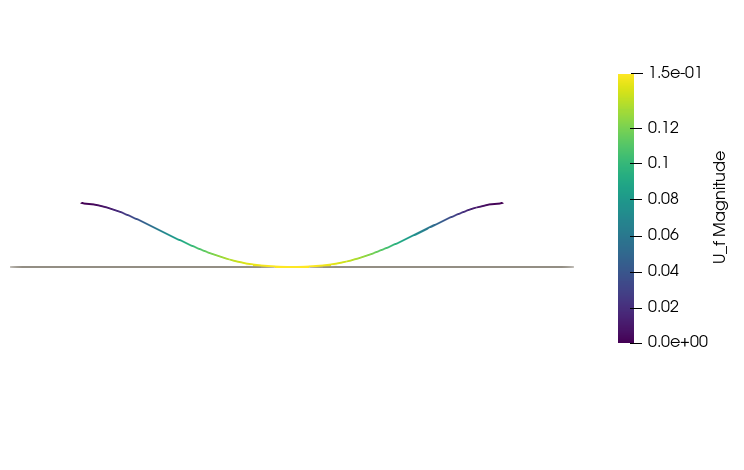
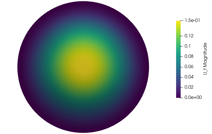
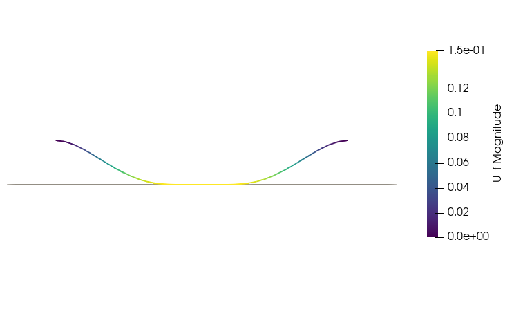
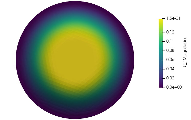
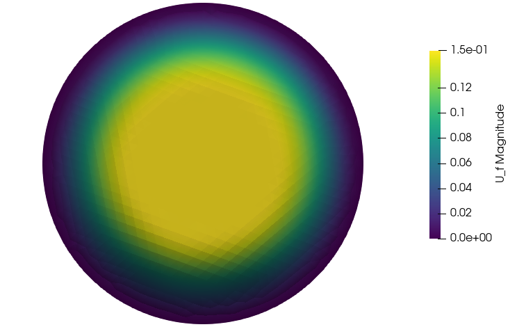
The results of these experiments are reported in Figure 12 below.
(a)
(b)
(a)
(b)
(a)
(b)
(a)
(b)
(a)
(b)
(a)
(b)
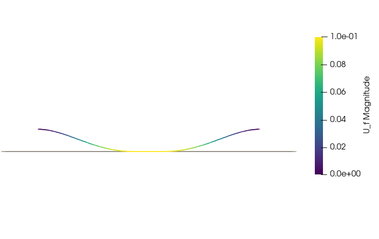
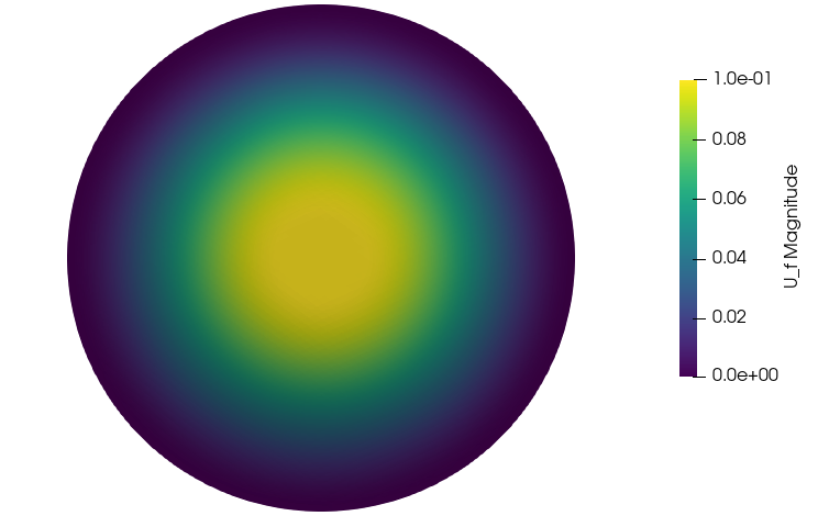
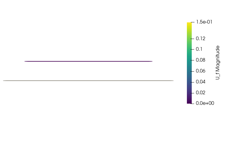
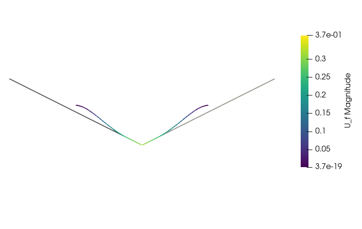
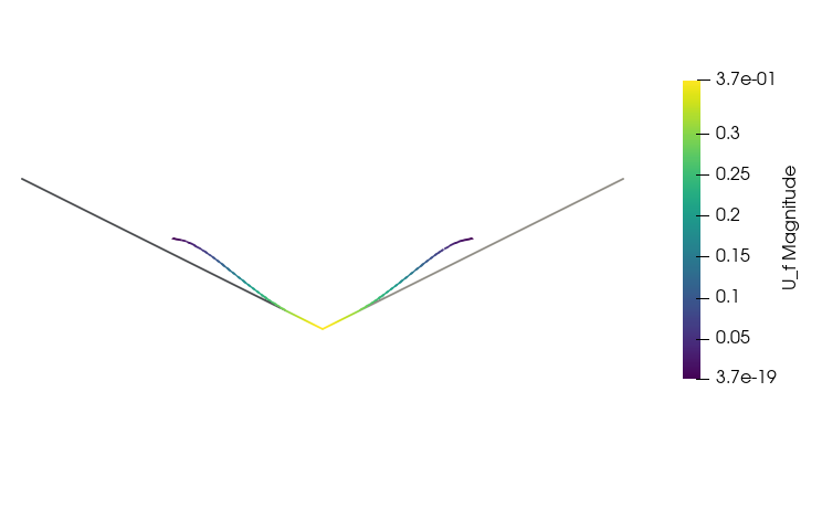
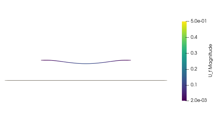
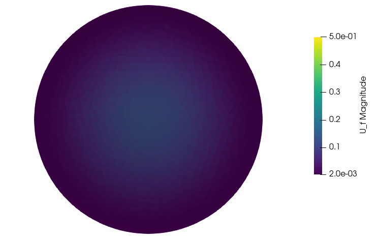
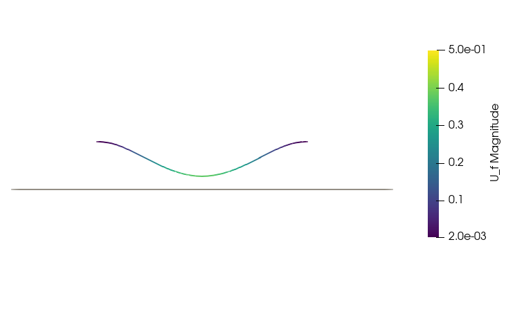
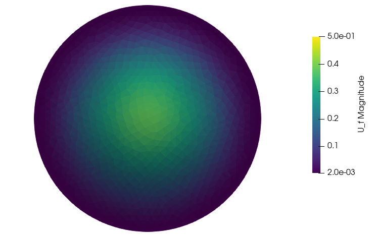
Figure 12. Cross sections of a deformed membrane shell subjected not to cross a given planar obstacle.
Given and we observe that as the applied body force magnitude increases the contact area increases.
We also constrain solution of Problem to remain confined above the function defined by two planes:
The applied body force density entering the model is the same given by
where is a non-negative integer.
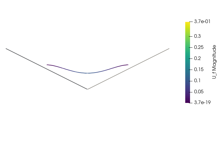
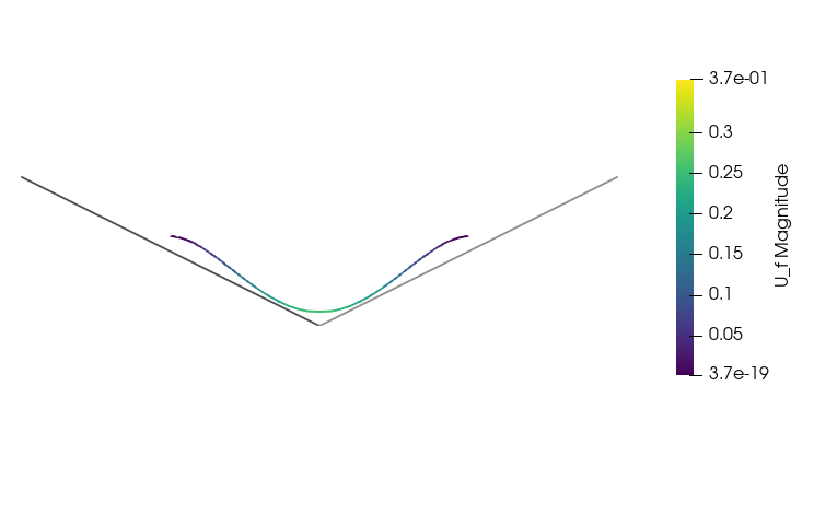
The results of these experiments are reported in Figure 15 below.
(a)
(b)
(a)
(b)
(a)
(b)
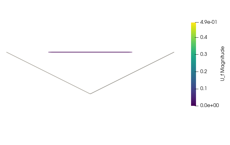
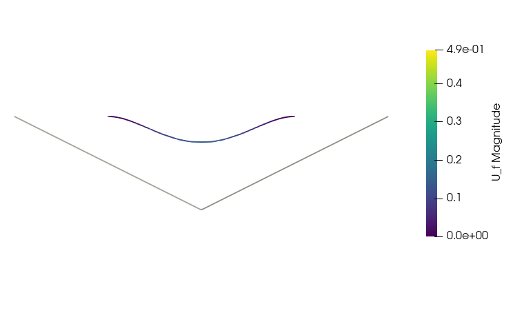
Figure 15. Cross sections of a deformed membrane shell subjected not to cross a given planar obstacle.
Given and we observe that as the applied body force magnitude increases the contact area increases.
4. Numerical approximation of an obstacle problem for linearly elastic shallow shells. The general case
In this section, we denote by a simply connected Lipschitz domain.
Following [19] (see also Section 3.1 of [11]), we now recall the rigorous definition of a linearly elastic shallow shell (from now on, shallow shell for the sake of brevity).
Assume that, for each , it is given a function that defines the middle surface of the corresponding shallow shell with thickness equal to .
According to the shallowness criterion (cf., e.g., [11]), a linearly elastic shell is shallow if and only if there exists a function , independent of , such that:
(11)
The relation in (11) means that, up to an additive constant, the deviation of the middle surface of the reference configuration of the shallow shell from a plane, which is measured via the function , is of the same order as the thickness of the shell.
The middle surface of the corresponding shallow shell is thus parametrised in Cartesian coordinates by the mapping defined by:
The shallow shells we are considering in this section are all made of a homogeneous and isotropic material, they are clamped on their entire lateral boundary, and they are subjected to the action of applied body forces only. For what concerns surface traction forces, the mathematical models characterised by the confinement condition considered in this paper (confinement condition which is also considered in [35] in a less complex geometrical framework) do not take any surface traction forces into account.
Indeed, there could be no surface traction forces applied to the portion of the shell surface that engages contact with the obstacle. The elastic behaviour of the shallow shell is then described by means of its two Lamé constants and (cf., e.g., [10]).
The function space over which the original problem is posed is the following (cf., e.g., [11]):
The geometrical constraint we subject the shallow shell to amounts to requiring that the reference configuration of the shell and its admissible deformations remain confined in a prescribed half-space, which is identified with a unit-vector that belongs to the orthogonal complement of the plane identifying one such half-space and that points towards the prescribed half-space.
The obstacle the shallow shell does not have to cross is thus identified with the plane describing the boundary of the half-space where the shallow shell has to remain confined. As we shall see next, the corresponding confinement condition will have to bear at once on all the components of the displacement vector field.
The confinement condition we are here considering is more general than the one considered in the papers [35, 36], where the authors required the shallow shell to lie above the plane .
The assumption on the geometry of the obstacle made in [35, 36] allowed the exploitation of the fact that the solution of the equilibrium problem for shallow shells is a Kirchhoff-Love field so as to “separate” the variational inequalities governing the variations in the transverse component of the displacement vector field from the variational equations governing the variations in the tangential components of the displacement vector field.
Apart from this, the assumptions on the geometry of the obstacle made in [35, 36] ensured the convergence of the Finite Element Method proposed in [47] for approximating the solution of the obstacle problem studied in [35, 36].
For more general obstacle geometries like the ones we are considering in this section, the “separation” of the tangential components of the displacement vector field from the transverse component of the displacement vector field does not hold, in general. Moreover, it appears that the techniques proposed in [47] are not applicable to the case where the confinement condition hinges at once on all the components of the displacement vector field.
For the sake of notational compactness, define the space associated with the tangential components of the displacement vector field
Let . Therefore, we can write:
The displacement vector field must thus to the following subset of the space :
The subscript “K”in the definition of the set aptly recalls the connection of the model we are studying with Koiter’s model [31, 32, 33], which is posed over the same functional space.
Let us observe that the set is non-empty as in view of the assumption (12). It is also straightforward to observe that the set is closed and convex.
Let be given once and for all, and define the set:
Let denote a generic point in the set , with .
We are now ready to state the de-scaled two-dimensional limit obstacle problem - akin to the one recovered in [35, 36] - governing the deformation of shallow shells subjected to remaining confined in a prescribed half-space. Note that, differently from other linearly elastic shells models that are formulated in curvilinear coordinates, we are here opting for a formulation in Cartesian coordinates, since it is judicious to regard shallow shell models as “more similar” to linearly elastic plate models rather than to linearly elastic shell models.
Problem .
Find satisfying:
for all , where
We also make the following assumptions on the scalings of the applied body forces. Recall that these scalings are justified by the rigorous asymptotic analysis carried out in [11]. Let us define . We assume that there exist functions independent of such that the following assumptions on the data hold:
(13)
Note that the left-hand side of the variational inequalities in Problem is associated with the symmetric, continuous and -elliptic (cf., e.g., Theorem 3.6-1 of [11]) bilinear form given by (cf. Sections 3.5, 3.6 and 3.7 of [11]):
A straightforward computation shows that:
for all .
Likewise, we associate the sum of the right-hand sides of the variational inequalities in Problem with a linear and continuous form defined as follows:
Therefore, Problem admits a unique solution . Equivalently, we have that is the unique element in the set that minimises the energy functional
over the set .
In order to numerically approximate the solution of Problem via the Finite Element Method, we first state the penalised version of Problem , that will still be a fourth order problem, and we will then state the corresponding penalised mixed formulation, in the same fashion as what has been done in section 2.
Once again, we denote by a positive penalty parameter that is meant to approach zero. Define the mapping by:
For each , consider the following penalised energy functional:
The penalty term we inserted into the expression for the energy functional is meant to prefer equlibria that satisfy the geometrical constraint according to which the shell has to remain confined in the prescribed half-space, in order to prevent the blow-up of the corresponding penalised energy.
The penalised version of Problem is denoted by , and takes the following form.
Problem .
Find satisfying:
for all .
Since the operator defined beforehand is clearly hemi-continuous and strongly monotone, since the bilinear form is -elliptic, and since the linear form is continuous, an application of the Minty-Browder Theorem (cf., e.g., Theorem 9.14-1 in [14]) ensures the existence and uniqueness of solutions for Problem . Equivalently, this means that, for a given , there exists a unique element such that
At this point, we observe that a discretisation of Problem via the Finite Element Method is not possible without resorting to conforming or non-conforming Finite Elements for approximating the transverse component of the displacement vector field. Therefore, this kind of formulation is not amenable as the latter Finite Elements are currently not implemented in a number of Finite Element Analysis.
One could think to directly work on the approximation of the solution of the original variational inequalities stated in Problem via Enriching Operators, following the ideas in [47]. However, pursuing this strategy would eventually let the following problems arise. First, enriched Finite Elements for fourth order problems are currently not implemented in a number of Finite Element Analysis libraries and, second, the techniques developed in [47] seem to work only when the geometrical constraint is solely expressed in terms of the transverse component of the displacement vector field. Therefore, in light of the latter statement, it seems that the techniques presented in [47] are not applicable to the case we are considering, which is the case where the obstacle is a generic plane and the constraint hinges at once on all the components of the displacement vector field.
In order to overcome these difficulties, we introduce - in the same fashion as section 2 - a mixed formulation for Problem . Prior to doing so, however, we need to assume - as in section 2 - that there exists a vector field such that a.e. in (cf., e.g., Theorem 6.14-1 in [14]).
Problem .
Find satisfying:
for all , where
Clearly, Problem admits a unique solution as a re-writing of Problem . It is straightforward to observe that the set is non-empty, closed and convex, and that the components of the tensor are linear and continuous with respect to the natural norm of the vector space .
In the same fashion as in section 2, we add a further penalty term which is meant to steer the solutions towards states where the dual variable is as close as possible to the gradient of the transverse component of the primal variable and, finally, a harmonic corrector so as to lay out the foundations to establish the existence and uniqueness for the solutions of the variational problem announced below.
Problem .
Find such that a.e. in , and satisfying:
for all such that a.e. in .
As a remark, we observe that the choice for the powers of the parameter - which, we recall, is regarded as fixed - made in Problem and Problem are derived from the de-scalings descending from the asymptotic analysis carried out in Theorem 3.5-1 of [11]. We anticipate that these de-scalings will play no role in determining the convergence of the numerical schemes for approximating the solution of Problem . As a result of the de-scalings for Problem , we consider the following regularity-preserving natural de-scalings for the solutions of Problem below:
(14)
We now establish the existence an uniqueness of solutions for Problem . The first step to achieve this goal consists in establishing the coerciveness of the left-hand side of the variational equations appearing in Problem by means of an inequality of Korn’s type in mixed coordinates. Critical to establishing this estimate is the assumed simple connectedness of the Lipschitz domain , which will allow us to apply the weak Poincaré lemma (cf., e.g., Theorem 6.17-4 of [14]).
Theorem 4.1.
Let be a simply connected Lipschitz domain. Let be given.
Then, there exists a constant such that:
for all such that a.e. in .
Proof.
Let and define the space . For each , define the tensor as follows (cf., e.g., Theorem 3.4-1 of [11]):
Let us recall that a generalised inequality of Korn’s type (cf., e.g., Theorem 3.4-1 of [11] for the notation appearing in the next inequality) with homogeneous Dirichlet boundary conditions on gives that there exists a constant such that:
Observe that the symmetry of implies that a.e. in .
An application of the weak Poincaré lemma (cf., e.g., Theorem 6.17-4 of [14]) gives that there exists a function such that
(15)
and, moreover, any other function such that a.e. in is of the form , for some constant .
Observe that, since and that on , we can apply Lemma 8.1 in [4] on each of the overlapping local charts covering the boundary of the boundary so as to infer that is constant along . Letting we obtain that .
In light of (15), we are in a position to define the vector field as follows:
Therefore, it is immediate to verify the following identities:
Note that the last equality in the algebraic manipulation of the terms descends as a result of the assumed symmetry for . We denote by the components of the tensor introduced in Problem in the special case where .
A straightforward computation gives
(16)
on the one hand. On the other hand, the definition of gives that:
(17)
Combining (16), (17) and the generalised Korn’s inequality in Theorem 3.4-1 of [11] and the standard Poincaré-Friedrichs inequality (cf., e.g., Theorem 6.5-2 of [14]), we obtain that:
The proof is complete by letting .
∎
We are now ready to establish the existence and uniqueness of solutions for Problem .
Theorem 4.2.
For each and for each , Problem admits a unique solution . Besides, we have that the following convergences hold
where is the unique solution of Problem .
Proof.
In light of the Korn inequality in mixed coordinates (Theorem 4.1), the shallowness criterion (11), and the de-scalings (14), we have that there exists a constant independent of such that:
(18)
An application of the Pincaré-Friedrichs inequality, (18), the monotonicity of the operator (cf., e.g., [48]), and an application of the fact that give that the non-linear operator associated with the left-hand side of the variational equations in Problem is strongly monotone with respect to the natural norm of the space . Combining this with the linearity of the form of the right-hand side of the variational equations in Problem puts us in a position to apply the Minty-Browder Theorem (cf., e.g., Theorem 9.14-1 of [14]) so as to infer that Problem admits a unique solution.
Specialise in the variational equations of Problem . We obtain that an application of (18) and Young’s inequality [53] gives:
Therefore, we obtain that
(19)
where the right-hand side is independent of , and is also independent of in light of the scalings for the applied body forces (13).
In light of (19), we obtain that
(20)
and that:
(21)
In view of (19)–(21), we have that, up to passing to a subsequence,
(22)
As a result of the linearity and continuity of the divergence operator, we obtain that:
(23)
Besides, combining (19) and (20) with the triangle inequality gives:
(24)
Thanks to the de-scalings (14), the right-hand side of (24) is bounded independently of and . Thanks to the classical Poincaré-Friedrichs inequality (cf., e.g., Theorem 6.5-2 in [14]), we have that, up to passing to a subsequence, the following weak convergence takes place:
(25)
Combining the estimate (21) with (22), (25), the Rellich-Kondrašov Theorem (cf., e.g., Theorem 6.6-3 in [14]), and the strong monotonicity and Lipschitz continuity of the operator (cf., e.g., [48]), we obtain that in , so that:
Combining the second and third convergences in (22) with (25), and applying the Fatou Lemma gives
(27)
so that in . The fact that is a Lipschitz domain in turn gives that so that or, equivalently, that .
The last thing to show is that the weak limit is in fact the unique solution of Problem or, equivalently, that is the unique solution of Problem . To this aim, let us test the variational equations in Problem at , where is chosen arbitrarily in . We obtain that:
(28)
Passing to the as , and applying the Fatou Lemma gives:
(29)
Since , we have that:
(30)
Passing to the as in (28), and exploiting the convergences (22)–(27) and (29), (30), we obtain that:
(31)
for all . We have thus shown that converges to the unique solution of the mixed variational inequalities in Problem .
∎
For sufficiently smooth given data and for a sufficiently smooth boundary , the solution of Problem enjoys higher regularity up to the boundary, in the sense that (cf., e.g., [26] and [42]):
(32)
Because of the presence of the harmonic corrector, the classical theory for the augmentation of regularity (cf., e.g., [40] and [42]), and the fact that the constraint is inactive near the boundary [45, 47], it results:
The problem of approximating the solution of Problem via the Finite Element Method is not as straightforward as the prototypical problem discussed in section 2. The reason for this is that, in general, the symmetry of the gradient matrix of the dual variable cannot be handled directly by means of an ad hoc Finite Element. Let us how how the theory of fluid mechanics (cf., e.g., [28, 50]) helps us overcome this difficulty.
Define the vector space
and define the function by:
The operator switch is clearly well-defined, linear, bounded and isometric.
Therefore, the operator switch is one-to-one.
It is also easy to see that the operator switch is onto, and we thus observe that the operator switch is an isometric isomorphism, whose inverse is once again an isometric isomorphism and is given by:
Let us observe that, if , then . This leads us to consider the vector space
which is widely used in the treatment of the Stokes equations and of the Navier-Stokes equations (cf., e.g., [28] and [50]).
For the purpose of approximating the solution of Problem , we need to show that can be identified with . To this aim, it suffices to observe that is an isometric isomorphism.
Therefore, numerically approximating vector fields with symmetric gradient is equivalent to numerically approximating vector fields with vanishing divergence. The advantage of the latter approach is due to the plethora of available results in the context of the study of the Stokes equations and Navier-Stokes equations. Indeed, according to page 74 and formula (1.49) in [50], we have that:
where , for all smooth enough, and we recall that .
Let denote the parameter associated with the mesh size of an affine regular triangulation of the Lipschitz domain . Let be the finite-dimensional subspace of associated with a triangulation made of Hsieh-Clough-Tocher Finite Elements (cf., e.g., Chapter 6 in [9]).
For each , we can thus define the space
as well as the space:
We have that the following density result holds.
Theorem 4.3.
Assume that is triangulated by means of an affine regular triangulation.
Assume that the space is discretised by means of a conforming Finite Element.
Then, the following density result holds:
Proof.
Let . We have that there exists a unique such that .
Given any , there exists a function , for small enough, such that . Defining , we have that and that
where is the continuity constant associated with the operator. Thanks to the arbitrariness of , the proof is complete.
∎
An immediate consequence of Theorem 4.3 is that the elements in can be approximated by means of an ad hoc conforming Galerkin method. Note that the previous proof is not in general true if the discretisation of the space is performed via non-conforming Finite Elements.
For each , let us denote by a finite-dimensional space of associated with an affine regular triangulation made of Courant triangles.
We are thus in a position to write down the discretisation of Problem .
Problem .
Find satisfying:
for all .
The existence and uniqueness of solutions for Problem can be established in the same fashion as Theorem 2.3, as an application of the Minty-Browder Theorem (cf., e.g., Theorem 9.14-1 in [14]).
The next result establishes the convergence of the solution of Problem to the solution of Problem .
If we iterate once more the augmentation-of-regularity argument (cf., e.g., [26]) exploiting the fact that , we can infer that so that it immediately follows that .
Theorem 4.4.
Let be the solution of Problem .
Let be the solution of Problem .
Then,
Proof.
In what follows, we denote by
where is the standard interpolation operator. We denote by and the two-dimensional and three-dimensional analogues of .
In light of the variational equations of Problem , the variational equations of Problem , Young’s inequality [53] and Hölder’s inequality, we have that:
Thanks to Korn’s inequality in mixed coordinates (Theorem 4.1) and the classical Poincaré-Friedrichs inequality (cf., e.g., Theorem 6.5-2 in [14]), we have that:
where is a positive constant which only depends on and , the fourth-last inequality descends from an application of Theorem 3.1-6 in [9] and the fact that the operator switch is an isometric isomorphism, the third-last inequality is due to the continuity of the operator, the second-last inequality follows from the remarks preceding Theorem 4.4 and an application of Theorem 6.1.3 in [9] with .
The last equality descends from the fact that and the fact that the switch operator is an isometric isomorphism.
Since the variational problems we are interested in were derived as a result of a de-scaling for the unknowns (14), we have that the constant estimates the semi-norms in the last inequality and depends on and the scaled forcing term only.
Applying the de-scalings (14) on the last term in the previous block of estimates gives
so that:
The conclusion follows immediately.
∎
We note in passing that if we let , with gives that the solution of Problem converges to the solution of Problem as .
One of the main difficulties we encountered for showing that the solution of Problem converges to the solution of Problem is that it is not possible to define the interpolation operator for vector fields in with symmetric gradient matrix. However, thanks to the isomorphisms associated with the switch and operators and the theory presented in [28, 50], we can consider the interpolation operator for the space , which can be approximated by means of the Finite Element space associated with Hsieh-Clough-Tocher triangles. We can then transform the interpolation function defined over the space into a function of .
This is, in fact, the function that we exploit to derive the estimates that put in a position to apply Cea’s Lemma (cf., e.g., Theorem 2.4.1 in [9]).
Another issue that appears in the derivation of the estimates in Theorem 4.4 is the regularity requirement for the stream function , which has to be at least of class .
Note that this kind of augmentation of regularity is totally licit for the penalised problem, even though it is not licit, in general, for the transverse component of the solution of the variational inequalities in Problem to enjoy a regularity higher than in light of the results in [5, 6].
We observe that, with the current state of the art for a number of Finite Element Analysis libraries, the model governed by Problem cannot be implemented numerically as the typical installations of the aforementioned libraries do not come with conforming Finite Elements for fourth order problems.
In the next section we show that, for a flat surface, the theory in [28, 50] is not necessary in order to devise the error estimates for the approximation of the solution of the mixed penalised problem. The reason for this is that the standard Korn’s inequality (cf., e.g, Theorem 6.15-4) will in fact suffice to establish the uniform ellipticity ensuring the existence and uniqueness of solutions for the analogue of Problem for the surface under consideration.
5. Numerical approximation of an obstacle problem for linearly elastic shallow shells. The case of a flat surface
Let us now assume that the function parametrising the middle surface of the hierarchy of linearly elastic shallow shells considered in section 4 is constant in , i.e., there exists a constant such that:
It is straightforward to see that the components of the strain tensor in mixed coordinates reduce to the standard symmetrised gradient with respect to the primal variable, namely,
As a result, the inequality of Korn’s type in mixed coordinates established in Theorem 4.1 reduces to the standard Korn’s inequality in (cf., e.g., Theorem 6.15-4 of [14]) and it is thus not necessary to assume the symmetry of the gradient matrix for the dual variable in order to establish one such inequality.
Observe that the inequality of Korn’s type in mixed coordinates established in Theorem 4.1 required the assumption that the gradient matrix of the dual variable was symmetric to compensate the lack of rigidity for surfaces which are compatible with the definition of shallow shells. Indeed, differently from other types of linearly elastic shells (e.g., linearly elastic elliptic membrane shells [17, 18] or linearly elastic flexural shells [23]) for which a rigidity theorem is available for the corresponding two-dimensional limit models recovered as a result of a rigorous asymptotic analysis, the two-dimensional limit model for shallow shells does not enjoy, in general, one such rigidity property.
The case where the surface modelling the geometry of the shallow shell under consideration is flat constitutes an example where one such rigidity property is regained.
The penalised version of Problem , in the case where , thus takes the following simpler form.
Problem .
Find satisfying:
for all , where
In the same fashion as section 4, Problem , which is simply a rewriting of Problem in the case where in , admits a unique solution.
In the same fashion as section 4, we can state the penalised version of Problem .
Problem .
Find satisfying:
for all .
Moreover, in the same fashion as section 4, the following result can be established.
Theorem 5.1.
For each and for each , Problem admits a unique solution . Besides, we have that the following convergences hold
where is the unique solution of Problem .
Proof.
Clearly, Problem admits a unique solution thanks to the classical Korn’s inequality (cf., e.g., Theorem 6.15-4 in [14]), the classical Poincaré-Friedrichs inequality (cf., e.g., Theorem 6.5-2 in [14]), and the strong monotonicity of the non-linear term (cf., e.g., [48]), which put us in a position to apply the Minty-Browder Theorem (cf., e.g., Theorem 9.14-1 in [14]). Note in passing that the proof for the existence and uniqueness of solutions for Problem does not hinge on the inequality of Korn’s type in mixed coordinates (Theorem 4.1).
The proof for the convergence result follows the same strategy as in Theorem 4.2.
∎
The main advantage brought forth by the fact that no symmetry for the gradient matrix of the dual variable is required to establish the existence and uniqueness of solutions for Problem is that the discretisation of Problem via the Finite Element Method can be carried out by sole means of Courant triangles, i.e., without resorting to the theory in [28, 50], that was instead essential to establish the convergence of the Finite Element approximation described in section 4.
Recalling that, for each , we denote by a finite-dimensional subspace of , the discretised version of Problem takes the following form.
Problem .
Find satisfying:
for all .
The convergence of the solution of Problem to the solution of Problem descends straightforwardly from the same computations as in Theorem 4.4.
Theorem 5.2.
Let be the solution of Problem .
Let be the solution of Problem .
Then,
Proof.
Since the proof closely follows the strategy of Theorem 4.4, we just limit ourselves to sketch it.
Thanks to the classical Korn’s inequality (cf., e.g., Theorem 6.15-4 in [14]) and the classical Poincaré-Friedrichs inequality (cf., e.g., Theorem 6.5-2 in [14]), we have that:
where is a positive constant which only depends on and , and the second-last inequality descends from an application of Theorem 3.1-6 of [9], and the last inequality descends from the standard augmentation-of-regularity results (cf., e.g., [42]) and the de-scalings (14). Once again, since the variational problems we are interested in were derived as a result of a de-scaling for the unknowns (14), we have that the constant estimates the semi-norms in the last inequality and depends on and the scaled forcing term only.
The completion of the proof follows by observing that the latter chain of inequalities gives:
∎
In particular, we observe that the coupling with ensures the convergence of the solution of Problem to the solution of Problem as .
6. Numerical experiments simulating the displacement of linearly elastic shallow shells subjected to an obstacle
In this last section of the paper, we implement numerical simulations aiming to validate the theoretical results presented in section 5.
Consider as a domain a circle of radius , and denote one such domain by :
Throughout this section, the values of , and are fixed once and for all as follows:
The parametrisation for the middle surface of the linearly elastic shallow shell under consideration is given by:
(33)
We define the unit-norm vector orthogonal to the plane constituting the obstacle by . The applied body force density entering the first two batches of experiments is given by , where
The numerical simulations are performed by means of the software FEniCS [34] and the visualization is performed by means of the software ParaView [1].
The plots were created by means of the matplotlib libraries from a Python 3.9.8 installation.
The first batch of numerical experiments is meant to validate the claim of Theorem 5.1. After fixing the mesh size , we let tend to zero in Problem . Let and be two solutions of Problem , where and .
The solution of Problem is discretised component-wise by Courant triangles (cf., e.g., [9]) and homogeneous Dirichlet boundary conditions are imposed for all the components.
At each iteration, Problem is solved by Newton’s method. The algorithm stops when the error is smaller than .
Error
6.0e-09
5.3e-07
3.0e-09
2.7e-07
1.5e-09
1.3e-07
7.5e-10
6.6e-08
3.7e-10
3.3e-08
1.9e-10
1.7e-08
9.3e-11
8.3e-09
(a)
(b)Error convergence as for . Original figure.
Error
1.5e-09
5.0e-07
7.5e-10
2.5e-07
3.7e-10
1.3e-07
1.9e-10
6.3e-08
9.3e-11
3.1e-08
4.7e-11
1.6e-08
2.3e-11
7.8e-09
(a)
(b)Error convergence as for . Original figure.
Error
3.7e-10
5.0e-07
1.9e-10
2.5e-07
9.3e-11
1.3e-07
4.7e-11
6.3e-08
2.3e-11
3.1e-08
1.2e-11
1.6e-08
5.8e-12
7.8e-09
(a)
(b)Error convergence as for . Original figure.
Error
9.3e-11
5.0e-07
4.7e-11
2.5e-07
2.3e-11
1.2e-07
1.2e-11
6.2e-08
5.8e-12
3.1e-08
2.9e-12
1.5e-08
1.5e-12
7.7e-09
(a)
(b)Error convergence as for . Original figure.
Figure 19. Given , the first component of the solution of Problem converges with respect to the standard norm of as .
From the data patterns in Figure 19 we observe that, for a given mesh size , the solution of Problem converges as . This is coherent with the conclusion of Theorem 5.1.
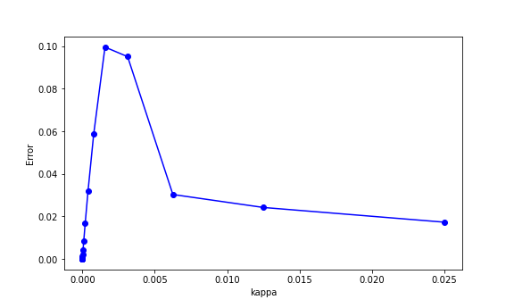
The second batch of numerical experiments is meant to validate the claim of Theorem 5.2.
We show that, for a fixed as in Theorem 5.2, the error residual tends to zero as .
The algorithm stops when the error residual of the Cauchy sequence is smaller than .
Once again, each component of the solution of Problem is discretised by Lagrange triangles (cf., e.g., [9]) and homogeneous Dirichlet boundary conditions are imposed for all the components and, at each iteration, Problem is solved by Newton’s method.
The results of these experiments are reported in Figure 21 below.
(a)For the algorithm stops after 25 iterations
(b)For the algorithm stops after 41 iterations
(a)For the algorithm stops after 46 iterations
(b)For the algorithm stops after 47 iterations
Figure 21. Given as in Theorem 5.2, the error converges to zero as . As increases, the number of iterations needed to meet the stopping criterion of the Cauchy sequence increases.
The third batch of numerical experiments validates the genuineness of the model from the qualitative point of view.
We observe that the presented data exhibits the pattern that, for a fixed and a fixed , the contact area increases as the applied body force intensity increases.
For the third batch of experiments, the applied body force density entering the model is given by , where is a non-negative integer and
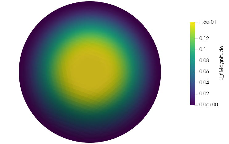
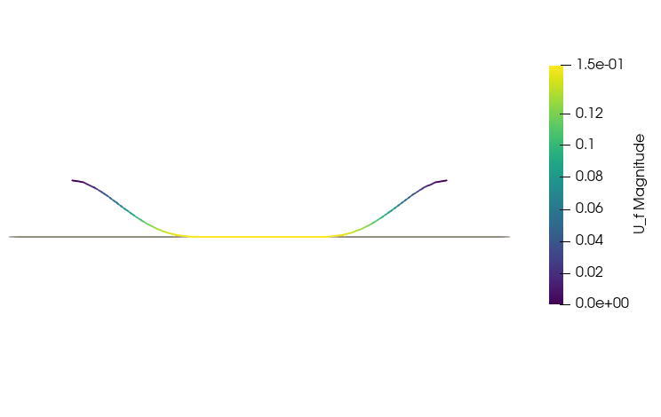
The results of these experiments are reported in Figure 27 below.
(a)
(b)
(a)
(b)
(a)
(b)
(a)
(b)
(a)
(b)
(a)
(b)
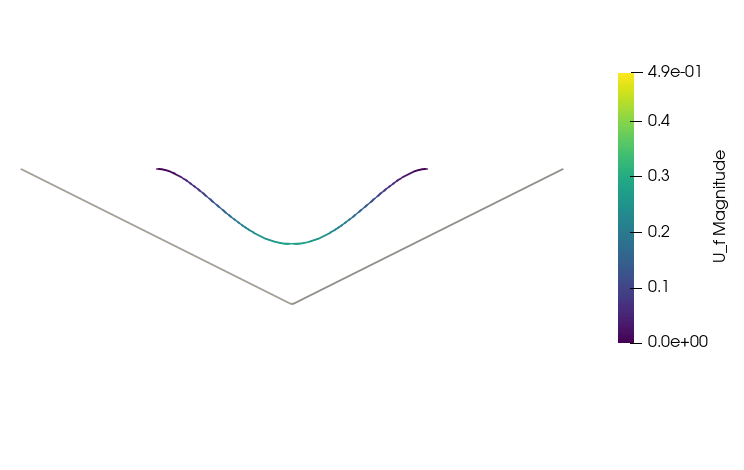
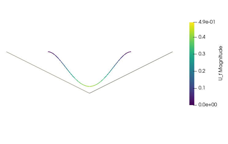
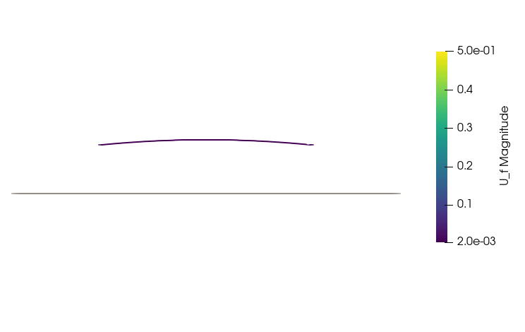
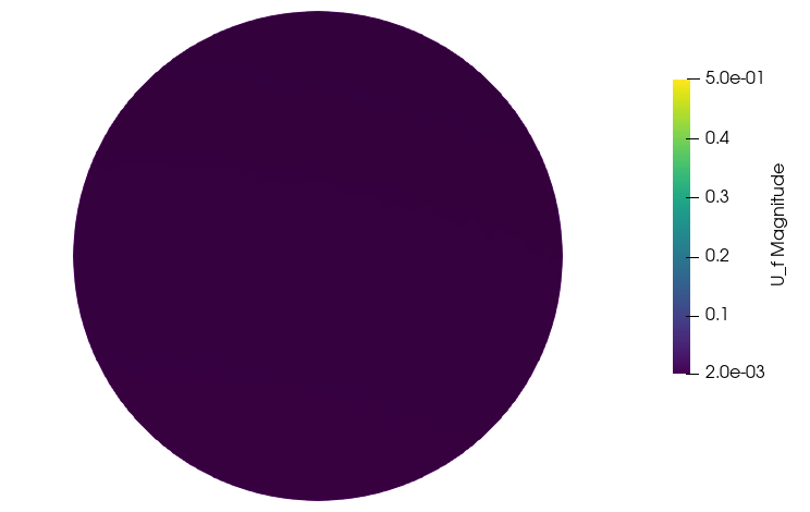
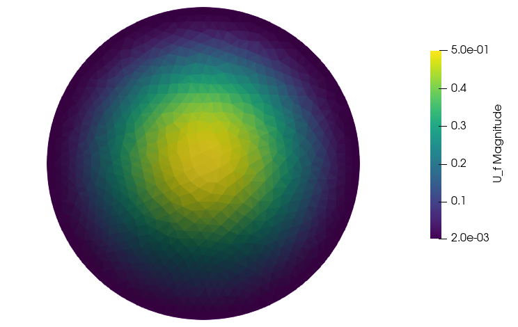
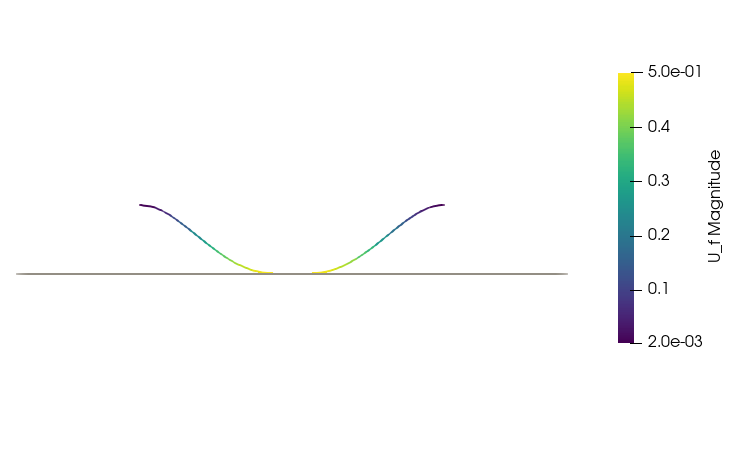
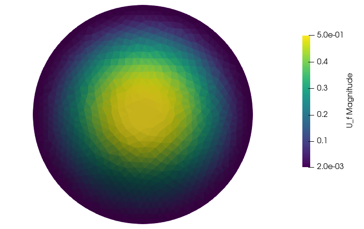
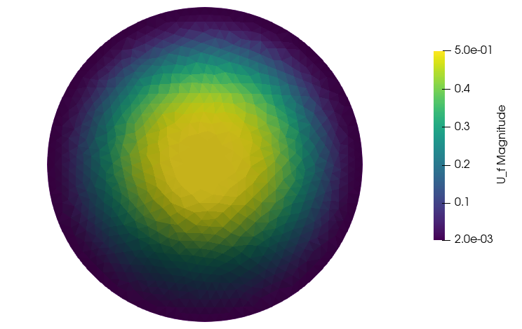
Figure 27. Cross sections of a deformed membrane shell subjected not to cross a given planar obstacle.
Given and we observe that as the applied body force magnitude increases the contact area increases.
We also constrain the shell to remain confined in the convex portion of Euclidean space identified by the planes . The unit-normal vectors in the orthogonal complement of these two planes are given by
respectively.
The applied body force density entering the model is given by , where is a non-negative integer and
where is a non-negative integer.
The results of these experiments are reported in Figure 30 below.
(a)
(b)
(a)
(b)
(a)
(b)
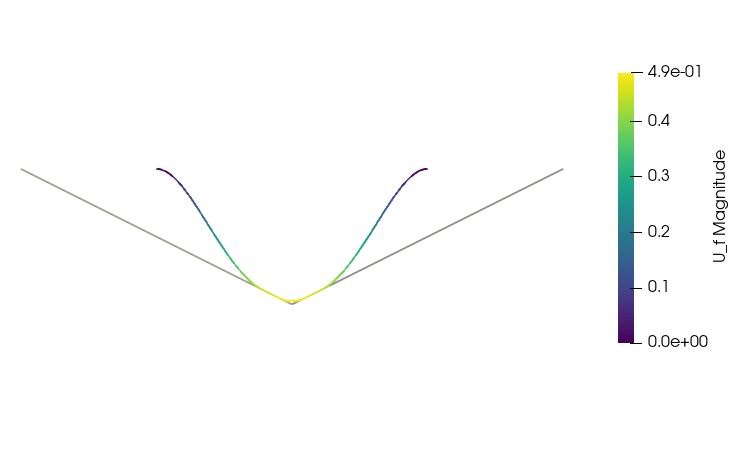
Figure 30. Cross sections of a deformed membrane shell subjected not to cross a given planar obstacle.
Given and we observe that as the applied body force magnitude increases the contact area increases.
For the sake of completeness, we also conduct the same experiment as above in the case where the middle surface of the linearly elastic shallow shell under consideration has non-zero curvature. We recall that this is the case where the symmetry for the gradient matrix of the dual variable has to be taken into account. The experiments, in this case, are carried out by means of the software FreeFem [30], as this is one of the few Finite Element Analysis libraries111For a complete overview of the features of the most popular Finite Element Analysis libraries, see the website https://en.wikipedia.org/wiki/List_of_finite_element_software_packages whose installation come with Hsieh-Clough-Tocher triangles. We recall that Hsieh-Clough-Tocher triangles are used to discretise the stream function resulting from an application of the weak Poincaré lemma (cf., e.g., Theorem 6.17-4 of [14]). The applied body force density entering the model is given by , where is a non-negative integer and:
The numerical results are presented in Figure 36 below.
(a)
(b)
(a)
(b)
(a)
(b)
(a)
(b)
(a)
(b)
(a)
(b)
Figure 36. Cross sections of a deformed membrane shell subjected not to cross a given planar obstacle.
Given and we observe that as the applied body force magnitude increases the contact area increases.
Conclusions and Commentary
In this paper, we proposed a new mixed Finite Element Method for approximating the solution of obstacle problems governed by fourth order differential operators. First, we presented the method for a prototypical obstacle problem for the biharmonic operator, and we performed numerical experiments to corroborate the theoretical results we established. The method we proposed generalises the results in the papers [22] and [16], as the finite-dimensional space where the approximation is carried out is - in our case - a subspace of the space where the mixed formulation is posed.
Second, we moved to the study of the numerical approximation of an obstacle problem for linearly elastic shallow shells constrained to remain confined in a prescribed half-space. In order to establish the existence and uniqueness for the penalised mixed variational formulation related to the original problem, we had to establish a preliminary inequality of Korn’s type in mixed coordinates, whose validity hinges on the fact that the gradient matrix of the dual variable is symmetric. In order to handle the latter constraint in the context of the numerical approximation of the solution by means of a Finite Element Method, we observed that there is a connection between the current analytical framework and the analytical framework of fluid mechanics; more precisely, the analytical framework of incompressible fluids. The numerical approximation by means of the Finite Element Method was successful, although the stream function had to be approximated by means of a conforming Finite Element for fourth order problems like, for instance, Hsieh-Clough-Tocher triangles. As a result of this, we have shown that there are mixed Finite Element Methods for fourth order problems that still necessitate finite elements to perform the discretisation of the solution. Moreover, we observe that the latter fact appears to be related to the lack of rigidity of the middle surface of linearly elastic shallow shells, for which a two-dimensional rigidity theorem is not available, unlike the linearly elastic shells discussed in [12].
Third, and finally, we considered an example of linearly elastic shallow shell whose middle surface is flat. We observed that, in this case, the existence and uniqueness of solutions for the penalised mixed formulation descends from the standard Korn’s inequality. This in turn implies that the symmetry of the gradient matrix of the dual variable no longer has to be required for the competitors to the role of solution for the variational problem under consideration, and the discretisation of the penalised mixed formulation by Finite Elements can thus be performed by means of Courant triangles. Numerical tests are performed for corroborating the theoretical results we obtained beforehand.
Declarations
Authors’ Contribution
All the authors equally contributed to the realisation of each part of this manuscript.
Acknowledgements
This paper was started during the time P.P. held a position as a Zorn Psotdoctoral Fellow at Indiana University Bloomington. P.P. and T.S. are greatly thankful to Professor Roger M. Temam, in his capacity of Director of the Institute for Scientific Computing and Applied Mathematics, for allowing them to perform part of the numerical experiments presented in this manuscript on the supercomputer of his Institute.
Ethical Approval
Not applicable.
Availability of Supporting Data
Not applicable.
Competing Interests
All authors certify that they have no affiliations with or involvement in any organization or entity with any competing interests in the subject matter or materials discussed in this manuscript.
Funding
Not applicable.
References
Ahrens et al. [2005]
J. Ahrens, B. Geveci, and C. Law.
ParaView: An End-User Tool for Large Data
Visualization.
Visualization Handbook, Elsevier, 2005.
ISBN-13: 978-0123875822.
Aragón and Duarte [2023]
A. Aragón and C. A. Duarte.
Fundamentals of Enriched Finite Element Methods.
2023.
Brenner et al. [2013]
S. Brenner, L. Sung, H. Zhang, and Y. Zhang.
A Morley finite element method for the displacement obstacle
problem of clamped Kirchhoff plates.
J. Comput. Appl. Math., 254:31–42, 2013.
Brezis [2011]
H. Brezis.
Functional Analysis, Sobolev Spaces and Partial
Differential Equations.
Springer, New York, 2011.
Caffarelli and Friedman [1979]
L. A. Caffarelli and A. Friedman.
The obstacle problem for the biharmonic operator.
Ann. Scuola Norm. Sup. Pisa Cl. Sci. (4),
6:151–184, 1979.
Caffarelli et al. [1982]
L. A. Caffarelli, A. Friedman, and A. Torelli.
The two-obstacle problem for the biharmonic operator.
Pacific J. Math., 103:325–335, 1982.
Carstensen and Köler [2017]
C. Carstensen and K. Köler.
Nonconforming fem for the obstacle problem.
IMA J. Numer. Anal., 37(1):64–93,
2017.
Carstensen et al. [2021]
C. Carstensen, S. Gaddam, N. Nataraj, A. K. Pani, and D. Shylaja.
Morley finite element method for the von Kármán obstacle
problem.
ESAIM Math. Model. Numer. Anal., 55(5):1873–1894, 2021.
Ciarlet [1978]
P. G. Ciarlet.
The Finite Element Method for Elliptic Problems.
North-Holland, Amsterdam, 1978.
Ciarlet [1988]
P. G. Ciarlet.
Mathematical Elasticity. Vol. I: Three-Dimensional Elasticity.
North-Holland, Amsterdam, 1988.
Ciarlet [1997]
P. G. Ciarlet.
Mathematical Elasticity. Vol. II: Theory of Plates.
North-Holland, Amsterdam, 1997.
Ciarlet [2000]
P. G. Ciarlet.
Mathematical Elasticity. Vol. III: Theory of Shells.North-Holland, Amsterdam, 2000.
Ciarlet [2005]
P. G. Ciarlet.
An Introduction to Differential Geometry with
Applications to Elasticity.
Springer, Dordrecht, 2005.
Ciarlet [2013]
P. G. Ciarlet.
Linear and Nonlinear Functional Analysis with Applications.
Society for Industrial and Applied Mathematics, Philadelphia, 2013.
Ciarlet and Glowinski [1975a]
P. G. Ciarlet and R. Glowinski.
Dual iterative techniques for solving a finite element approximation
of the biharmonic equation.
Comput. Methods Appl. Mech. Engrg., 5:277–295,
1975a.
Ciarlet and Glowinski [1975b]
P. G. Ciarlet and R. Glowinski.
Dual iterative techniques for solving a finite element approximation
of the biharmonic equation.
Comput. Methods Appl. Mech. Engrg., 5:277–295,
1975b.
Ciarlet and Lods [1996a]
P. G. Ciarlet and V. Lods.
On the ellipticity of linear membrane shell equations.
J. Math. Pures Appl., 75:107–124,
1996a.
Ciarlet and Lods [1996b]
P. G. Ciarlet and V. Lods.
Asymptotic analysis of linearly elastic shells. I. Justification
of membrane shell equations.
Arch. Rational Mech. Anal., 136(2):119–161, 1996b.
Ciarlet and Miara [1992]
P. G. Ciarlet and B. Miara.
Justification of the two-dimensional equations of a linearly elastic
shallow shell.
Comm. Pure Appl. Math., 45(3):327–360,
1992.
Ciarlet and Piersanti [2019a]
P. G. Ciarlet and P. Piersanti.
Obstacle problems for Koiter’s shells.
Math. Mech. Solids, 24:3061–3079,
2019a.
Ciarlet and Piersanti [2019b]
P. G. Ciarlet and P. Piersanti.
A confinement problem for a linearly elastic Koiter’s shell.
C.R. Acad. Sci. Paris, Sér. I, 357:221–230,
2019b.
Ciarlet and Raviart [1974]
P. G. Ciarlet and P.-A. Raviart.
A mixed finite element method for the biharmonic equation.
In Mathematical aspects of finite elements in partial
differential equations (Proc. Sympos., Math. Res. Center, Univ.
Wisconsin, Madison, Wis., 1974), pages 125–145. Academic Press, New
York-London, 1974.
Ciarlet et al. [1996]
P. G. Ciarlet, V. Lods, and B. Miara.
Asymptotic analysis of linearly elastic shells. II. Justification
of flexural shell equations.
Arch. Rational Mech. Anal., 136(2):163–190, 1996.
Ciarlet et al. [2018]
P. G. Ciarlet, C. Mardare, and P. Piersanti.
Un problème de confinement pour une coque membranaire
linéairement élastique de type elliptique.
C. R. Math. Acad. Sci. Paris, 356(10):1040–1051, 2018.
Ciarlet et al. [2019]
P. G. Ciarlet, C. Mardare, and P. Piersanti.
An obstacle problem for elliptic membrane shells.
Math. Mech. Solids, 24(5):1503–1529, 2019.
Evans [2010]
L. C. Evans.
Partial Differential Equations.
American Mathematical Society, Providence, Second edition, 2010.
Gazzola et al. [2024]
F. Gazzola, V. Pata, and C. Patriarca.
Attractors for a fluid-structure interaction problem in a
time-dependent phase space.
J. Funct. Anal., 286(2):Paper No. 110199,
56, 2024.
Girault and Raviart [1986]
V. Girault and P.-A. Raviart.
Finite element methods for Navier-Stokes equations,
volume 5 of Springer Series in Computational Mathematics.
Springer-Verlag, Berlin, 1986.
Theory and algorithms.
Gong et al. [2019]
S. Gong, S. Wu, and J. Xu.
New hybridized mixed methods for linear elasticity and optimal
multilevel solvers.
Numer. Math., 141(2):569–604, 2019.
Hecht [2012]
F. Hecht.
New development in FreeFem ++.
Numer. Math., 20(3–4):251–265, 2012.
Koiter [1959]
W. T. Koiter.
A consistent first approximation in the general theory of thin
elastic shells.
In Proc. Sympos. Thin Elastic Shells (Delft), pages 12–33,
Amsterdam, 1959. North-Holland.
Koiter [1966]
W. T. Koiter.
On the nonlinear theory of thin elastic shells. I, II, III.
Nederl. Akad. Wetensch. Proc. Ser. B, 69:1–17,
18–32, 33–54, 1966.
Koiter [1970]
W. T. Koiter.
On the foundations of the linear theory of thin elastic shells. I,
II.
Nederl. Akad. Wetensch. Proc. Ser. B 73 (1970),
169–182; ibid, 73:183–195, 1970.
Langtangen and Logg [2016]
H. P. Langtangen and A. Logg.
Solving PDEs in Python, volume 3 of Simula
SpringerBriefs on Computing.
Springer, Cham, 2016.
The FEniCS tutorial I.
Léger and Miara [2008]
A. Léger and B. Miara.
Mathematical justification of the obstacle problem in the case of a
shallow shell.
J. Elasticity, 90:241–257, 2008.
Léger and Miara [2010]
A. Léger and B. Miara.
Erratum to: Mathematical justification of the obstacle problem in
the case of a shallow shell.
J. Elasticity, 98:115–116, 2010.
Lewicka [2023]
M. Lewicka.
Calculus of variations on thin prestressed films—asymptotic
methods in elasticity, volume 101 of Progress in Nonlinear
Differential Equations and their Applications.
Birkhäuser/Springer, Cham, 2023.
Lions [1957]
J. L. Lions.
Lectures on elliptic partial differential equations.
In Tata Institute of Fundamental Research Lectures on
Mathematics, volume 10, pages iii+130+vi. 1957.
Ma and Wang [2019]
T. Ma and S. Wang.
Phase transition dynamics.
Springer, Cham, 2019.
Second edition of [ MR3154868].
Meixner and Piersanti [2024]
A. Meixner and P. Piersanti.
Numerical approximation of the solution of an obstacle problem
modelling the displacement of elliptic membrane shells via the penalty
method.
Appl. Math. Optim., 89(2):Paper No. 45,
60, 2024.
Miranville [2019]
A. Miranville.
The Cahn-Hilliard equation, volume 95 of CBMS-NSF
Regional Conference Series in Applied Mathematics.
Society for Industrial and Applied Mathematics (SIAM), Philadelphia,
PA, 2019.
Recent advances and applications.
Nečas [1967]
J. Nečas.
Les méthodes directes en théorie des équations
elliptiques.
Masson et Cie, Éditeurs, Paris; Academia, Éditeurs, Prague,
1967.
Piersanti [2022a]
P. Piersanti.
On the improved interior regularity of the solution of a second order
elliptic boundary value problem modelling the displacement of a linearly
elastic elliptic membrane shell subject to an obstacle.
Discrete Contin. Dyn. Syst., 42(2):1011–1037, 2022a.
Piersanti [2022b]
P. Piersanti.
Asymptotic analysis of linearly elastic elliptic membrane shells
subjected to an obstacle.
Journal of Differential Equations, 320:114–142,
2022b.
Piersanti [2022c]
P. Piersanti.
On the improved interior regularity of the solution of a fourth order
elliptic problem modelling the displacement of a linearly elastic shallow
shell subject to an obstacle.
Asymptot. Anal., 127(1–2):35–55,
2022c.
Piersanti [2023]
P. Piersanti.
Asymptotic analysis of linearly elastic flexural shells subjected to
an obstacle in absence of friction.
J. Nonlinear Sci., 33(4):Paper No. 58, 39,
2023.
Piersanti and Shen [2020]
P. Piersanti and X. Shen.
Numerical methods for static shallow shells lying over an obstacle.
Numer. Algorithms, 85(2):623–652,
2020.
Piersanti and Temam [2023]
P. Piersanti and R. Temam.
On the dynamics of grounded shallow ice sheets. modelling and
analysis.
Adv. Nonlinear Anal., 12(1):40 pp., 2023.
Rodríguez-Arós [2018]
A. Rodríguez-Arós.
Mathematical justification of the obstacle problem for elastic
elliptic membrane shells.
Applicable Anal., 97:1261–1280, 2018.
Temam [2001]
R. Temam.
Navier-Stokes equations.
AMS Chelsea Publishing, Providence, RI, 2001.
Theory and numerical analysis, Reprint of the 1984 edition.
Wu et al. [2024a]
R. Wu, X. Shen, D. Shi, and J. Yu.
Nonconforming finite element methods for two-dimensional linearly
elastic shallow shell model.
Adv. Appl. Math. Mech., 16(2):493–518,
2024a.
Wu et al. [2024b]
R. Wu, X. Shen, Q. Yang, and S. Zhu.
A new priori error estimation of nonconforming element for
two-dimensional linearly elastic shallow shell equations.
Commun. Math. Sci., 22(1):167–179,
2024b.
Young [1912]
W. H. Young.
On Classes of Summable Functions and their Fourier Series.
Proc. R. Soc. Lond. Ser. A Math. Phys. Eng.
Sci., 87:225–229, 1912.