CoSy: Evaluating Textual Explanations of Neurons

Abstract

A crucial aspect of understanding the complex nature of Deep Neural Networks (DNNs) is the ability to explain learned concepts within their latent representations. While various methods exist to connect neurons to textual descriptions of human-understandable concepts, evaluating the quality of these explanation methods presents a major challenge in the field due to a lack of unified, general-purpose quantitative evaluation. In this work, we introduce CoSy (Concept Synthesis)—a novel, architecture-agnostic framework to evaluate the quality of textual explanations for latent neurons. Given textual explanations, our proposed framework leverages a generative model conditioned on textual input to create data points representing the textual explanation. Then, the neuron’s response to these explanation data points is compared with the response to control data points, providing a quality estimate of the given explanation. We ensure the reliability of our proposed framework in a series of meta-evaluation experiments and demonstrate practical value through insights from benchmarking various concept-based textual explanation methods for Computer Vision tasks, showing that tested explanation methods significantly differ in quality. We provide an open-source implementation on GitHub.

Introduction

One of the key obstacles to the wider adoption of Machine Learning methods in various areas is the inherent opacity of modern Deep Neural Networks (DNNs)—in simple terms, we do not understand why these machines make the predictions they do. To address this problem, the field of Explainable AI (XAI) [1, 2] has emerged, to reveal the decision-making processes of DNNs in a human-understandable fashion. XAI has broadened its focus from explaining the decision-making of DNNs locally, i.e., for specific inputs using saliency maps [3, 4, 5, 6], to explaining the global behavior of the models by analyzing individual model components and their functional purpose [7]. Following the latter global explainability approach, often referred to as mechanistic interpretability [8, 9, 10], there are methods that aim to describe the specific concepts neurons have learned to detect [11, 12, 13, 14, 15, 16], enabling analysis of how these high-level concepts influence network predictions.

A popular approach for explaining the functionality of latent representations of a network is to label neurons using human-understandable textual concepts. A textual description is assigned to a neuron based on the concepts that the neuron has learned to detect or is significantly activated by. Over time, these methods have evolved from providing label-specific descriptions [11] to more complex compositional [12, 16] and open-vocabulary explanations [13, 15]. However, a significant challenge remains: the lack of a universally accepted quantitative evaluation measure for open-vocabulary neuron descriptions. As a consequence, different methods devised their own evaluation criteria, making it difficult to perform general-purpose, comprehensive cross-comparisons.

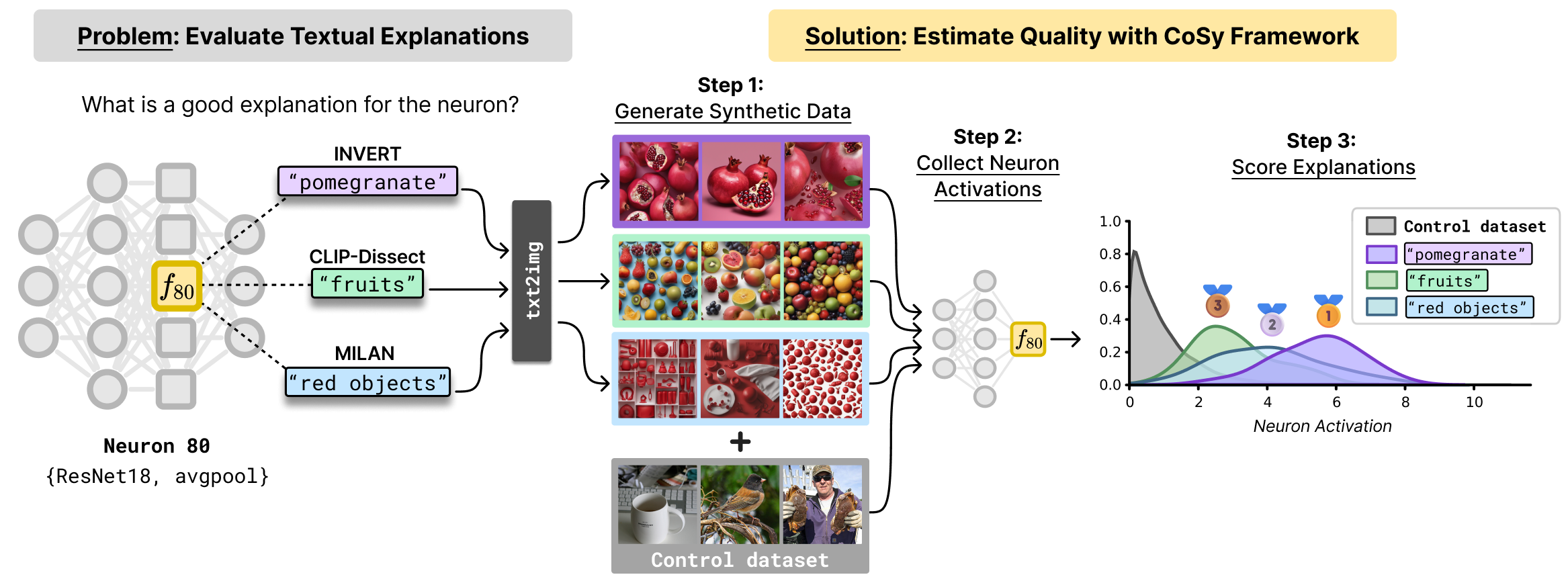
Figure 1: A schematic illustration of the CoSy evaluation framework for Neuron 80 in ResNet18’s avgpool layer. The current challenge lies in the absence of dataset- and architecture-agnostic evaluation measures to benchmark textual explanations of neurons. To address this, we propose CoSy, a framework consisting of three steps: first, a generative model translates textual concepts into the visual domain, creating synthetic images for each explanation using a text-to-image model. Then, inference is performed on synthetic images, along with a control image dataset, to collect neuron activations. Finally, by comparing the activations on synthetic images with activations on the control dataset, we can quantitatively assess the quality of the textual explanation and compare the results between different explanation methods. The implementation details of this example can be found in Appendix A.2.

With our work, we aim to bridge this gap by introducing a novel quantitative evaluation framework named CoSy, for evaluating open-vocabulary explanations for neurons in Computer Vision (CV) models (illustrated in Figure 1). Our approach builds on recent advancements in Generative AI, which enable the generation of synthetic images that align with provided concept-based textual explanations. We use a set of available text-to-image models to synthesize data points that are prototypical for specific target explanations. These data points allow us to evaluate how neurons differentiate between concept-related images and those from a control dataset. We summarize our contributions as below:

• We provide the first general-purpose, quantitative evaluation framework CoSy (Section 3) that enables the evaluation of individual or a set of textual explanation methods for CV models.

• In a series of meta-evaluation experiments (Section 4), we analyze the choice of generative models and prompts for synthetic image generation, demonstrating framework reliability.

• We benchmark existing explanation methods (Section 5) and extract novel insights, revealing substantial variability in the quality of explanations. Generally, textual explanations for lower layers are less accurate compared to those for higher layers.

Related Work

Activation Maximization

Activation Maximization is a commonly used methodology to understand what a neuron has learned to detect [17]. Such methods work by identifying input signals that trigger the highest activation in a neuron. This can be achieved synthetically, where an optimization process is employed to create the optimal input that maximizes the neuron’s activation [18, 19, 20], or naturally, by finding such inputs within a data corpus [21]. Activation Maximization has been employed for explaining latent representations of models [22, 23], including probabilistic models [24], detection of backdoor attacks [25] and spurious correlations [26]. Recently, it was shown that Activation Maximization methods could be manipulated to illustrate predetermined signals without significantly affecting performance [27, 28, 29]. However, one of the key limitations of this methodology lies in its inability to scale; its scalability is limited due to its dependency on users to manually audit maximization signals.

Automatic Neuron Interpretation

A more scalable alternative approach involves linking neurons with human-understandable concepts through textual descriptions. Network Dissection [11] (NetDissect) is a pioneering method in this field, associating convolutional neurons with a concept based on the Intersection over Union (IoU) of neuron activation maps and ground truth segmentation masks. Building on this, Compositional Explanations of Neurons (CompExp) [12] enhanced the detail of the explanations by allowing compositional concepts (i.e., concepts constructed using logical operators). MILAN [13] further expanded this by allowing for open-vocabulary explanations, permitting the generation of descriptions beyond predefined labels. INVERT [16] adopted a compositional concept approach, enabling explanations for general neuron types without relying on segmentation masks, and assigns compositional labels based on a neuron’s ability to distinguish concepts using the Area Under the Receiver Operating Characteristic Curve (AUC). FALCON [14] and CLIP-Dissect [15] compute image-text similarity with a CLIP model [30] for the most activating images and their corresponding captions or concept sets. An overview of the different techniques is illustrated in Table 1. More detailed descriptions of these methods can be found in Appendix A.1.

Prior Methods for Evaluation

While significant effort has been made towards developing approaches and tools for evaluating local explanations [31, 32, 33], there has been relatively limited focus on evaluating global methods. Currently, to the best of our knowledge, there is no unified approach that allows for benchmarking across models and explanation methods. In their respective papers, the INVERT and CLIP-Dissect explanation methods evaluated the accuracy of their explanations by comparing the generated neuron labels with ground truth descriptions provided for neurons in the output layer of a network. CLIP-Dissect additionally evaluates the quality of explanations by computing the cosine similarity in a sentence embedding space between the ground truth class name for each neuron and the explanation generated by the method. FALCON employs a human study conducted on Amazon Mechanical Turk to evaluate the concepts generated by the method. Participants are tasked with selecting the best explanation for each target feature from a selection of explanation methods, considering a given set of highly and lowly activating images. MILAN evaluates the performance of neuron labeling methods relative to human annotations using BERTScores [34].

Method

In the following section, we introduce CoSy—a first automatic evaluation procedure for open-vocabulary textual explanations for neurons. We first define preliminary notations in Section 3.1, then describe CoSy formally in Section 3.2.

Table 1: Comparison of characteristics of concept-based textual explanation methods. The columns (from left to right) represent the explanation method used, its textual output type (fixed-label, compositional, or open-vocabulary), the type of neuron targeted for analysis (convolutional, scalar, or predetermined), the target metric the method optimizes (IoU, WPMI, AUC, etc.), whether the method relies on auxiliary black-box models for finding or generating explanations (img2txt, CLIP), and whether the explanation method is architecture-agnostic, meaning it can be applied to any CV model. For a more detailed description of each method, refer to Appendix A.1.

Method	Explanation	Neuron Type	Target	Black-Box Dependency	Architecture-Agnostic
NetDissect [11]	fixed-label	conv.	IoU	—	✓
CompExp [12]	compositional	conv.	IoU	—	✓
MILAN [13]	open-vocabulary	conv.	WPMI	img2txt model	✓
INVERT [16]	compositional	scalar	AUC	—	✓
CLIP-Dissect [15]	open-vocabulary	scalar	SoftWPMI	CLIP	✓
FALCON [14]	open-vocabulary	predetermined	avg. CLIP score	CLIP	—

3.1 Preliminaries

Consider a Deep Neural Network (DNN) represented by the function $g:\mathcal{X}\rightarrow\mathcal{Z},$ where $\mathcal{X}\subset\mathbb{R}^{h\times w\times c}$ denotes the input image domain and $\mathcal{Z}\subset\mathbb{R}^{l}$ represents the model’s output domain. We can view the model as a composition of two functions, $F:\mathcal{X}\rightarrow\mathcal{Y},$ and $L:\mathcal{Y}\rightarrow\mathcal{Z},$ such that $g=L\circ F.$ Here $\mathcal{Y}\subset\mathbb{R}^{k\times w^{*}\times h^{*}}$, where $k\in\mathbb{N}$ is the number of neurons in the layer, and $w^{*},h^{*}\in\mathbb{N}$ represent the width and height of the feature map, respectively. The function $F,$ which we refer to as the feature extractor, can be chosen based on the layer of the model we aim to inspect. This could be an existing layer within the model or a concept bottleneck layer [35]. We refer to the $i$-th neuron within the layer as $f_{i}(\bm{x})=F_{i}(\bm{x}):\mathcal{X}\rightarrow\mathbb{R}^{w^{*}\times h^{*}}.$ Within the scope of this paper, we refer to explanation method as an operator $\mathcal{E}$ that maps a neuron to the textual description $s=\mathcal{E}(f_{i})\in\mathcal{S},$ where $\mathcal{S}$ is a set of potential textual explanations. The specific set of explanations depends on the implementation of the particular method.

3.2 CoSy: Evaluating Open-Vocabulary Explanations

A good textual explanation for a neuron should be a human-understandable description of an input that yields a high level of activation in the neuron. However, modern methods for explaining the functional purpose of neurons often provide open-vocabulary textual explanations, complicating the quantitative collection of natural data that represents the explanation. To address this issue, CoSy leverages recent advancements in generative models to synthesize data points that correspond to the textual explanation. The response of a neuron to a set of synthetic images is measured and compared to the neuron’s activation on a set of control natural images representing random concepts. This comparison allows for a quantitative evaluation of the alignment between the explanation and the target neuron.

Parameters of the proposed method include a control dataset $\mathbb{X}_{0}=\{\bm{x}^{0}_{1},\dots,\bm{x}^{0}_{n}\}\subset\mathcal{X},n\in\mathbb{N}$ – containing natural images that represent the concepts the model was originally trained on, a generative model $p_{M},$ that is used for synthesizing images, and a number of generated images $m\in\mathbb{N}.$ Given a neuron $f$ and explanation $s\in\mathcal{S},$ CoSy evaluates the alignment between the explanation and a neuron in 3 consecutive steps, which are illustrated in Figure 1.

1. Generate Synthetic Data. The first step involves generating synthetic images for a given explanation $s\in\mathcal{S},$ which we use as a prompt to a generative model $p_{M}$ to create a collection of synthetic images, denoted as $\mathbb{X}_{1}=\{\bm{x}^{1}_{1},\dots,\bm{x}^{1}_{m}\}\sim p_{M}(\bm{x}\mid s).$ This collection consists of $m\in\mathbb{N}$ images, where $m$ is adjustable as a parameter of the evaluation procedure.

2. Collect Neuron Activations. Given the control dataset $\mathbb{X}_{0}$ and the set of generated synthetic images $\mathbb{X}_{1}$, we collect activations as follows:

   $$\mathbb{A}_{0}=\{\sigma(f(\bm{x}^{0}_{1})),\dots,\sigma(f(\bm{x}^{0}_{n}))\}\in\mathbb{R}^{n},\mathbb{A}_{1}=\{\sigma(f(\bm{x}^{1}_{1})),\dots,\sigma(f(\bm{x}^{1}_{m}))\}\in\mathbb{R}^{m},$$ (1)

   where $\sigma$ is an aggregation function for multi-dimensional neurons. Within the scope of our paper, we use Average Pooling as aggregation function

   $$\sigma(\bm{y})=\frac{1}{w^{*}h^{*}}\sum_{i\in[1,w^{*}]}\sum_{i\in[1,h^{*}]}\bm{y}_{i,j},\quad\bm{y}\in\mathcal{Y}\subset\mathbb{R}^{w^{*}\times h^{*}}.$$ (2)

3. Score Explanations. The final step of the proposed method relies on the evaluation of the difference between neuron activations on the control dataset $\mathbb{A}_{0}$ and neuron activations given the synthetic dataset $\mathbb{A}_{1}.$ To quantify this difference, we utilize a scoring function $\Psi:\mathbb{R}^{n}\times\mathbb{R}^{m}\rightarrow\mathbb{R}$ to measure the difference between the distributions of activations.

In the context of our paper, we employ the following scoring functions:

• Area Under the Receiver Operating Characteristic (AUC)

  AUC is a widely used non-parametric evaluation measure for assessing the performance of binary classification. In our method, AUC measures the neuron’s ability to distinguish between synthetic and control data points

  $$\Psi_{\text{AUC}}(\mathbb{A}_{0},\mathbb{A}_{1})={\frac{\sum_{a\in\mathbb{A}_{0}}\sum_{{b\in\mathbb{A}_{1}}}{\textbf{1}}[a<b]}{|\mathbb{A}_{0}|\cdot|\mathbb{A}_{1}|}}.$$ (3)

• Mean Activation Difference (MAD)

  MAD is a parametric measure that quantifies the difference between the mean activation of the neuron on synthetic images and the mean activation on control data points

  $$\Psi_{\text{MAD}}(\mathbb{A}_{0},\mathbb{A}_{1})=\frac{1}{m}\sum_{b\in\mathbb{A}_{1}}b-\frac{1}{n}\sum_{a\in\mathbb{A}_{0}}a.$$ (4)

These two chosen metrics complement each other. AUC, being non-parametric and stable to outliers, evaluates the classifier’s ability to rank synthetic images higher than control images (with scores ranging from 0 to 1, where 1 represents a perfect classifier and 0.5 is random). On the other hand, MAD allows us to parametrically measure the extent to which images corresponding to explanations maximize neuron activation.

Meta-Evaluation Analysis

Meta-evaluation is the practice of evaluating the evaluation method itself [36]. This process is crucial to ensure the reliability of our proposed evaluation measure. In this section, we analyze the following: (1) which generative models and prompts provide the best similarity to natural images, (2) whether the model’s behavior on synthetic and natural images differs for the same concept, and (3) validating that CoSy provides appropriate evaluation scores for true and random explanations, given known ground truth concept for the neuron.

4.1 Synthetic Image Reliability

One of the key features of CoSy is its reliance on generative models to translate textual explanations of neurons into the visual domain. Thus, it is essential that the generated images reliably resemble the textual concepts. In the following section, we present an experiment where we varied several parameters of the generation procedure and evaluated the visual similarity between generated images and synthetic ones, focusing on concepts for which we have a collection of natural images.

For our analysis, we used only open-source and freely available text-to-image models, namely Stable Diffusion XL 1.0-base (SDXL) [37] and Stable Cascade (SC) [38]. We also varied the prompts for image generation. To measure the similarity between synthetic images and natural images corresponding to the same concept, we employed cosine similarity (CS) in the CLIP embedding space with the CLIP-ViT-B/32 model [30]. We select a set of 10 random concepts from the 1,000 classes in the ImageNet validation dataset [39]. For each [concept] we use 5 different prompts and employ them with SDXL and SC models, generating 50 images per concept. We then measure the CS between image pairs of the same class.

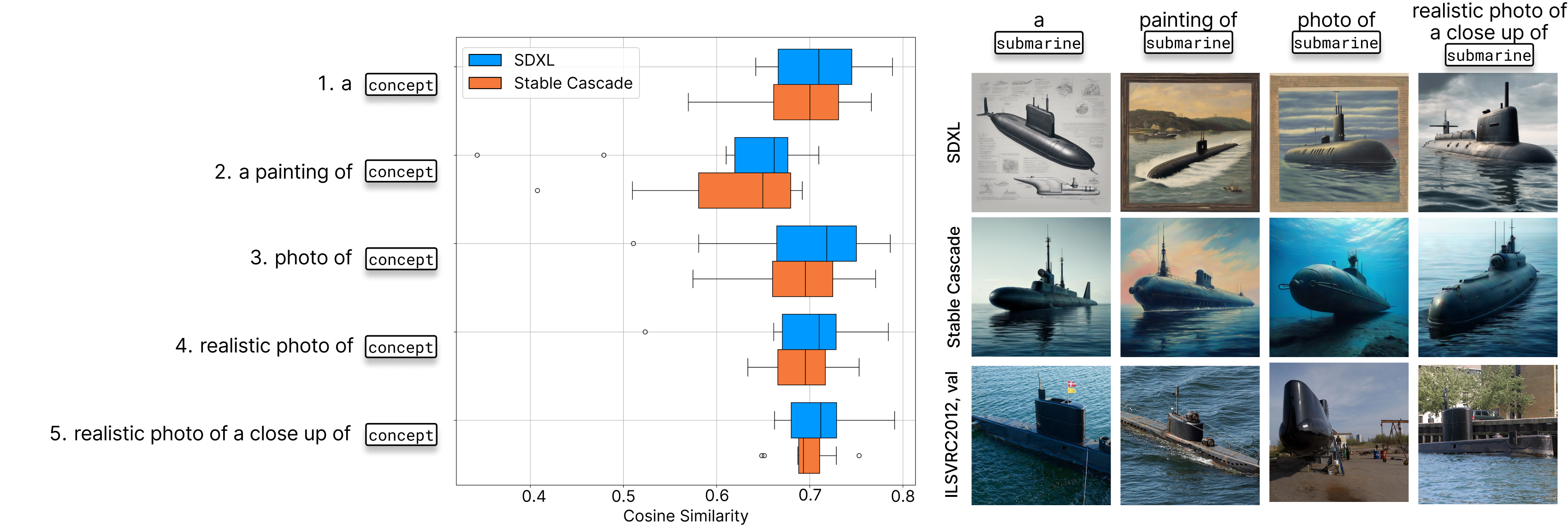
Figure 2: An overview of the impact of varying the prompt on the similarity between natural and synthetic images, using two text-to-image models. Left: average Cosine similarity (CS) across all natural and synthetic images over all classes are reported. Higher CS values are better, indicating greater similarity between the images. Right: an illustration of the visual differences produced by the SDXL and SC models in response to diverse prompts for the explanation concept “submarine”, and natural images from the ImageNet validation set. Our results show that SDXL and SC generate similar images, with SDXL generally being more closely aligned with natural images than SC.

Figure 2 illustrates the comparison across all generative models and prompts in terms of CS of generated images to natural images of the same class. The results indicate that when using prompt 5 as input to SDXL, the synthetic images show the highest similarity to natural images. The performance is generally best with the most detailed prompt (5) and closely aligns with prompts 1, 3, and 4. Moreover, SDXL appears to be slightly more effectively realizing detailed prompts than SC. As anticipated, the poorly constructed prompt (2) results in the lowest similarity to natural images for both models. If not stated otherwise, for all following experiments, prompt 5 together with SDXL model was employed for image generation.

4.2 Do Models Respond Differently to Synthetic and Natural Images?

Given the visual similarity between natural and synthetic images of the same concepts, we investigate whether CV models respond differently to these groups and if the activation differences indicate adversarial behavior. To this end, we employed four different models pre-trained on ImageNet: ResNet18 [40], DenseNet161 [41], GoogleNet [42], and ViT-B/16 [43]. For each model, we randomly selected 10 output classes and generated 50 images per class using the class descriptions. We pass both synthetic and natural images through the models, collecting the activations of the output neuron corresponding to each class.

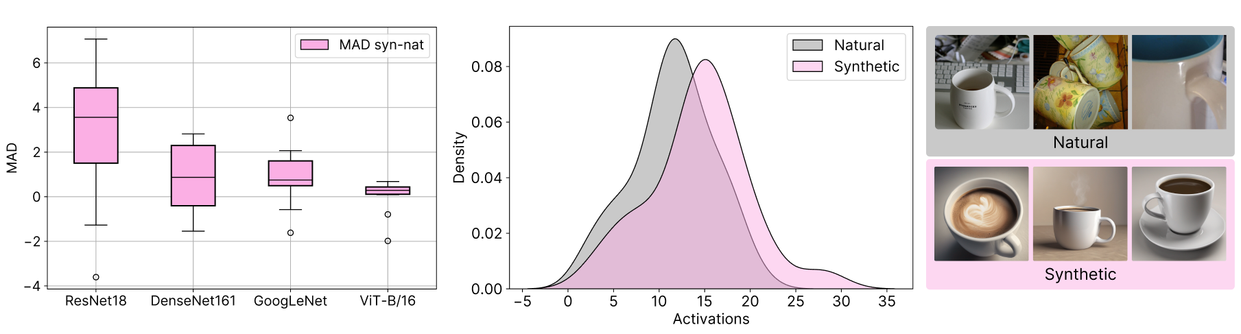
Figure 3: An overview of analyses performed to study the similarity between natural and synthetic images. From left to right: (1) an overview of MAD scores between synthetic and natural image activations of the output neuron’s ground truth classes for each model studied in this work, (2) activations collected for neuron 504 in ResNet18 for the class “coffee mug”, showcasing the difference between the natural and synthetic distributions and (3) examples of natural versus synthetic images. In both analyses, we observe a substantial overlap in the activations of synthetic and natural images, suggesting that the models respond similarly to both types of images.

Figure 3 (left) illustrates the distributions of the MAD between synthetic and natural images for the same class across the 10 classes. Generally, we observe that the activation of synthetic images is slightly higher than that of natural images of the same class. However, this difference is small, given the 0 value lies within 1 standard deviation. We also illustrated (Figure 3, right) the activations of neuron 504 in the ResNet18 output layer, corresponding to the “coffee mug” class. The results indicate a strong overlap in the neural response to both synthetic and natural images. While synthetic images activate the neuron slightly more, this doesn’t constitute an artifactual behavior or affect our framework, which we demonstrate in the following experiment.

4.3 Sanity Check

Table 2: Comparison of true and random explanations on output neurons with known ground truth labels. This table presents the quality estimates for true explanations, derived from target class labels, and random explanations, derived from randomly selected synthetic image classes (excluding the target class), across four models pre-trained on ImageNet. Higher values are better. Our results consistently show high scores for true explanations and low scores for random ones.

Model	AUC ($\uparrow$)		MAD ($\uparrow$)
	True	Random	True	Random
ResNet18	0.94$\pm$0.20	0.48$\pm$0.23	15.95$\pm$6.88	-0.53$\pm$2.00
DenseNet161	0.95$\pm$0.17	0.52$\pm$0.24	15.27$\pm$5.88	-0.13$\pm$1.55
GoogLeNet	0.95$\pm$0.16	0.40$\pm$0.19	8.98$\pm$3.48	-0.41$\pm$0.57
ViT-B/16	0.97$\pm$0.11	0.52$\pm$0.16	7.55$\pm$2.69	-0.00$\pm$0.21

A robust evaluation metric should reliably discern between random explanations resulting in low scores and non-random explanations resulting in high scores. To assess our evaluation framework regarding this requirement, we evaluated the results of the CoSy evaluation by comparing the scores of ground truth explanations with those of randomly selected explanations.

Following the experimental setup in Section 4.2, we selected a set of 10 output neurons and compared the CoSy scores of the ground truth explanations, given by the neuron label, with those of randomly selected explanations. The results, presented in Table 2, consistently demonstrate high scores for true explanations and low scores for random explanations. This experiment provides further evidence supporting the correctness of the proposed evaluation procedure. Additional experiments, including an analysis of the robustness of the evaluation measure, can be found in Appendix A.6.

Evaluating Explanation Methods

Within the scope of this section, we produce a comprehensive cross-comparison of various methods for the textual explanations of neurons. For this comparison, we employed models trained on different datasets, and we conducted our analysis on the latent layers of the models, where no ground truth is known.

5.1 Benchmarking Explanation Methods

In this section, we evaluated three recent textual explanation methods, namely MILAN, INVERT, and CLIP-Dissect. Our analysis involves four distinct models: two pre-trained on the ImageNet dataset [39] (ResNet18 [40], ViT-B/16 [43]) and two pre-trained on the Places365 dataset [44] (DenseNet161 [41], ResNet50 [40]). The ImageNet dataset focuses on objects, whereas the Places365 dataset is designed for scene recognition. Consequently, we customized our prompts accordingly: Prompt 5 performs best for object recognition, while for scene recognition, we found that Prompt 4 is more effective. Therefore, Prompt 4 was utilized in the Places365 experiment. For generating explanations with the explanation methods, we use a subset of 50,000 images from the training dataset on which the models were trained. For evaluation with CoSy, we use the corresponding validation datasets the models were pre-trained on as the control dataset. Additionally, for CLIP-Dissect, we define concept labels as a combination of the 20,000 most common English words and the corresponding dataset labels. For more details on Compute Resources refer to Appendix A.3.

Table 3: Benchmarking of explanation methods, explaining neurons on the second to last layers for different models. Explanations are generated with respect to a randomly selected set of 50 neurons where both AUC and MAD are reported. Higher values are better.

Dataset	Model	Layer	Method	AUC ($\uparrow$)	MAD ($\uparrow$)
ImageNet	ResNet18	Avgpool	MILAN	0.61$\pm$0.23	0.62$\pm$1.23
			INVERT	0.93$\pm$0.11	2.88$\pm$1.54
			CLIP-Dissect	0.93$\pm$0.11	3.45$\pm$1.71
	ViT-B/16	Features	MILAN	0.53$\pm$0.19	0.08$\pm$0.45
			INVERT	0.89$\pm$0.17	0.97$\pm$0.46
			CLIP-Dissect	0.78$\pm$0.19	0.76$\pm$0.62
Places365	DenseNet161	Features	MILAN	0.56$\pm$0.28	0.08$\pm$0.27
			INVERT	0.85$\pm$0.16	0.39$\pm$0.94
			CLIP-Dissect	0.82$\pm$0.21	0.41$\pm$1.04
	ResNet50	Avgpool	MILAN	0.65$\pm$0.28	0.35$\pm$0.53
			INVERT	0.94$\pm$0.08	1.04$\pm$0.74
			CLIP-Dissect	0.92$\pm$0.11	1.05$\pm$0.75

Results of the evaluation can be found in Table 3. Overall, INVERT achieves the highest AUC scores across all models and datasets, except for the ResNet18 applied to ImageNet where CLIP-Dissect achieves a similar score. Also across other models and datasets, CLIP-Dissect demonstrates consistently good results. Since INVERT optimizes AUC in explanation generation, it may be biased towards AUC in our evaluation, leading to higher scores. MILAN generally performs poorly, with an average AUC below 0.65 across all tasks, indicating performance close to random guessing. This is somewhat expected since MILAN works with convolutional neurons. MILAN tends to generate highly abstract explanations, such as “white areas”, “nothing” or “similar patterns”. These abstract concepts are particularly challenging for a text-to-image model to generate accurately, likely contributing significantly to the low scores of MILAN. Contrary to the AUC scores, the MAD scores suggest that CLIP-Dissect outperforms INVERT for convolutional neural networks applied to both datasets. Nonetheless, in these cases, INVERT concepts also achieve consistently high scores. Otherwise, we find similar outcomes for both metrics $\Psi$, with MILAN achieving poor scores in all experimental settings.

5.2 Explanation Methods Struggle to Explain Lower Layer Neurons

In addition to the general benchmarking, we aimed to study the quality of explanations for neurons in different layers of a model. Since it is well known that lower-layer neurons usually encode lower-level concepts [45], it is interesting to see whether explanation methods can capture the concepts these neurons detect. To investigate this, we examined the quality of explanations across layers 1 to 4 and the output layer of an ImageNet pre-trained ResNet18. In addition to three prior explanation methods, we included the FALCON method in our analysis. For more details on the implementation of FALCON and FALCON-original see Appendix A.1.4. For each layer, we randomly selected 50 neurons for analysis.

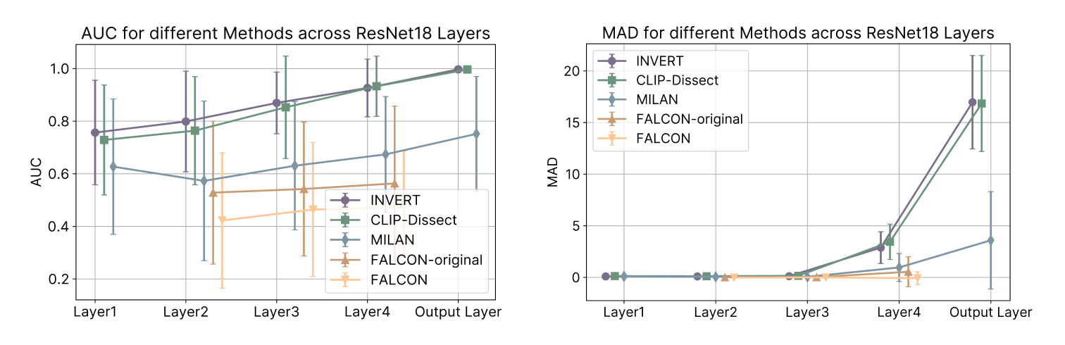
Figure 4: A comparison of how different explanation methods vary in their quality, as measured by AUC (left) and MAD (right), across different layers in ResNet18. INVERT and CLIP-Dissect similarly high AUC and MAD scores across all layers, while MILAN, FALCON, and FALCON-original scores are comparably low. Generally, all methods perform increasingly worse on lower layers.

In Figure 4 we present the AUC (left) and MAD (right) results for all explanation methods across layers $1$ to $4$ and the output layer of ResNet18. While less pronounced for the AUC metric, in general, we find increasing scores for later layers across all methods and both metrics $\Psi$, which suggest higher concept quality in later layers. Furthermore, we find that similar to the benchmarking experiments, MILAN achieves lower scores across metrics. However, here, FALCON scores the lowest, not even surpassing random performance indicated by its AUC results (AUC$<0.5$).

5.3 What are Good Explanations?

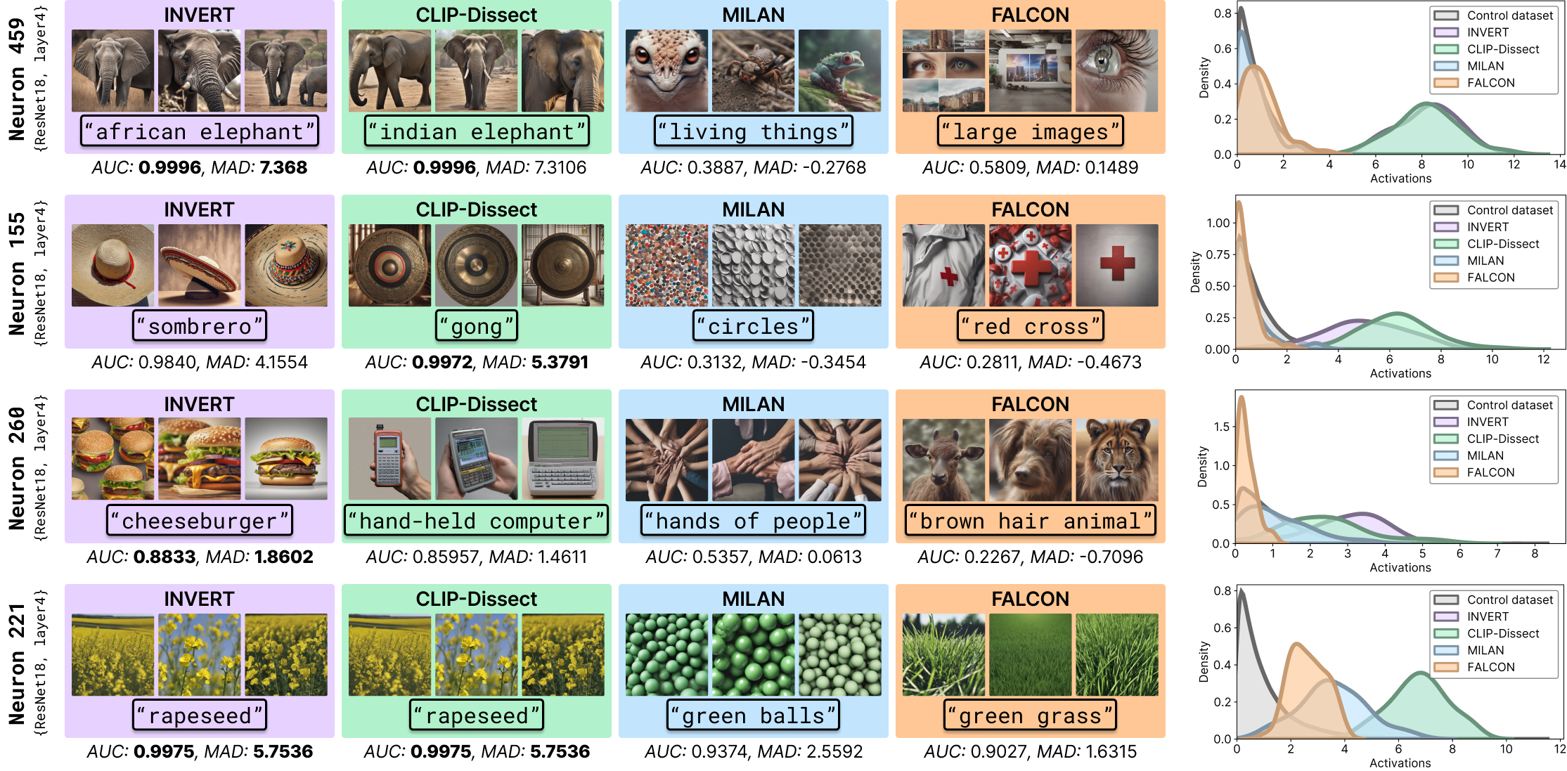
Figure 5: A qualitative example, of neuron explanations across $4$ neurons. The first four panels include the textual explanation across INVERT, FALCON, CLIP-Dissect, and MILAN alongside three corresponding generated images. The respective AUC and MAD scores are reported below each panel. The last panel shows the activation distributions across $50$ generated images for each method and the distribution of the control data.

In our approach, we assume that testing visual representations of textual explanations on neurons can provide insights into what constitutes good explanations. Based on this assumption, we observe consistently high results from CLIP-Dissect and INVERT. The qualitative examples in Figure 5 demonstrate that their explanations share visually similar concepts (neurons $155$ and $459$) or even identical concepts (neuron $221$) while both achieving high AUC and MAD scores. It is important to note that although INVERT performs slightly better in several tasks, its applicability is limited to input data labels. In contrast, CLIP-Dissect can generate labels from a broader selection of concepts, though its reliance on a black-box model reduces interpretability compared to INVERT.

There are instances, such as neuron $260$ in Figure 5, where all explanations vary significantly. In these cases, we find that the explanation activation distributions of FALCON and MILAN often overlap with or even match the control dataset, providing the user with nearly random explanations. This observation aligns with our overall findings: both the AUC and MAD scores consistently indicate the low performance of FALCON and MILAN explanations in CoSy evaluation. Also, neurons $459$ and $155$ demonstrate the gap between consistently higher and lower-performing explanation methods, with AUC scores of 0.5 and below suggesting that these explanations are essentially random guesses.

Conclusion

In this work, we propose the first automatic evaluation framework for concept-based textual explanations of neurons. Unlike existing ad-hoc evaluation methods, we can now quantitatively compare different concept-based textual explanation methods against each other and test, whether the given explanation describes the neuron accurately, based on the neurons’s activations. We can evaluate the quality of individual neuron explanations by examining how accurately they align with the generated concept data points, without requiring human involvement.

Our comprehensive meta-evaluation demonstrates that CoSy guarantees a reliable explanation evaluation. In several experiments, we show that concept-based textual explanation methods are most applicable for the last layers, where high-level concepts are learned. In these layers, INVERT and CLIP-Dissect provide high-quality neuron concepts, whereas MILAN and FALCON explanations have lower quality and can present close to random concepts, which might lead to wrong conclusions about the network. Thus, the results highlight the importance of evaluation when using concept-based textual explanation methods.

Limitations

While we can present promising results, one of the key limitations of CoSy is the generative model. For example, the text-to-image model training might not include the generated concepts. This absence leads to worsened generative performance but could be circumvented by an analysis of pre-training datasets and model performance. Moreover, the model’s capabilities of generating highly abstract concepts like “white objects” are limited. In both cases, exploring more sophisticated, specialized, or constrained models could help.

Future Work

Evaluation of non-local explanation methods is still a largely neglected research area, where CoSy plays an important yet preliminary part. In the future, we need additional, complementary definitions of explanation quality that extend our precise definition of AUC and MAD, e.g., that involve humans to assess plausibility [46] or evaluate explanation quality via the success of a downstream task [47]. Furthermore, we plan to extend the application of our evaluation framework to additional domains including NLP and healthcare. In particular, it would be interesting to analyze the quality of more recent autointerpretable explanation methods given by highly opaque, large language models (LLMs) [48, 9]. Also, we believe that applying CoSy to healthcare datasets, where the quality of the explanation really matter, is an impactful next step.

Appendix A Appendix

A.1 Concept-based Textual Explanation Methods

Concept-based textual explanation methods aim to provide insights into human-understandable concepts learned by DNNs, enabling a deeper understanding of their decision-making mechanisms. These methods provide textual descriptions for neurons in CV models. This creates a connection between the abstract representation of a concept by the neural network and a human interpretation. In general, a concept can be any abstraction, such as a color, an object, or even an idea [49]. Concept-based textual descriptions of a neuron $f_{i}$ can originate from various spaces depending on their generation process.

As defined in Section 3.1, we refer to explanation method as an operator $\mathcal{E}$ that maps a neuron to the textual description $s=\mathcal{E}(f_{i})\in\mathcal{S},$ where $\mathcal{S}$ is a set of potential textual explanations. The specific set of explanations depends on the implementation of the particular method. We define the following subsets of textual descriptions $s\in\mathcal{S}$:

• $\mathcal{C}$ represents the space of individual concepts,

• $\mathcal{L}$ represents the space of logical combinations of concepts,

• $\mathcal{N}$ represents the space of open-ended natural language concept descriptions.

These textual descriptions serve as explanations for $f_{i}$ generated by explanation methods.

Examples for such explanation methods are MILAN [13], FALCON [14], CLIP-Dissect [15], and INVERT [16]. Figure 6 shows the general principle of how $\mathcal{E}$ works. In Table 4 we outline the origin of textual descriptions and their corresponding set memberships for each $\mathcal{E}$.

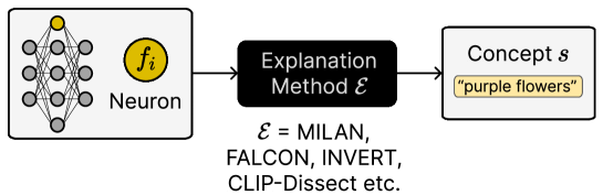
Figure 6: Concept-Based Textuaĺ Explanation Methods. A neural representation $f_{i}$ is selected, and a concept-based textual explanation method $\mathcal{E}$ is applied to generate a textual description $s$ explaining $f_{i}$.

Table 4: Set Membership and Origin of Descriptions. Generated textual descriptions $s$ have varying set membership and origin across all $\mathcal{E}$. These descriptions can originate from distinct spaces: individual concepts $\mathcal{C}$, logical combinations of concepts $\mathcal{L}$, and open-ended natural language concept descriptions $\mathcal{N}$. A labeled dataset refers to a collection of images paired with individual concept labels. Generated captions are produced by image-to-text models, such as Show-Attend-Tell [50]. An image caption dataset consists of image-caption pairs. A concept set consists of textual concept labels.

Method	Set	Origin
NetDissect	$\mathcal{C}$	labeled dataset
CompExp	$\mathcal{L}$	labeled dataset
MILAN	$\mathcal{N}$	generated caption
FALCON	$\mathcal{N}$	image caption dataset
CLIP-Dissect	$\mathcal{C}$	concept set
INVERT	$\mathcal{L}$	labeled dataset

A.1.1 NetDissect

Network Dissection (NetDissect) [11] is a method designed to explain individual neurons of DNNs, particularly convolutional neural networks (CNNs) within the domain of CV. This approach systematically analyzes the network’s learned concepts by aligning individual neurons with given semantic concepts. To perform this analysis, annotated datasets with segmentation masks are required, where these masks label each pixel in an image with its corresponding object or attribute identity. The Broadly and Densely Labeled Dataset (Broden) [11] combines a set of densely labeled image datasets that represent both low-level concepts, such as colors, and higher-level concepts, such as objects. It provides a comprehensive set of ground truth examples for a broad range of visual concepts such as objects, scenes, object parts, textures, and materials in a variety of contexts.

A concept $s\in\mathcal{C}\subset\mathcal{S}$ is defined as a visual concept in NetDissect and is provided by the pixel-level annotated Broden dataset. Given a CNN and the Broden dataset as input, NetDissect explains a neural representation $f_{i}$ by searching for the highest similarity between concept image segmentation masks and neuron activation masks. Concept image segmentation masks are provided by the Broden dataset $B_{s}({\boldsymbol{x}})\in\{0,1\}^{H\times W}$, where a value of 1 signifies the pixel-level presence of $s$, and 0 denotes its absence. Neuron activation masks are obtained by thresholding the continuous neuron activations of $f_{i}$ into binary masks $A({\boldsymbol{x}})\in\{0,1\}^{H\times W}$. Then the similarity $\delta_{\text{IoU}}$ between image segmentation masks and binary neuron masks can be evaluated using the Intersection over Union score (IoU) for an individual neuron within a layer:

$$\delta_{\text{IoU}}(f_{i},s)=\frac{\sum_{\boldsymbol{x}\in\boldsymbol{X}}\textstyle{\textbf{1}}\left(B_{s}(\boldsymbol{x})\cap A(\boldsymbol{x})\right)}{\sum_{\boldsymbol{x}\in\boldsymbol{X}}\textstyle{\textbf{1}}\left(B_{s}(\boldsymbol{x})\cup A(\boldsymbol{x})\right)}.$$ (5)

The NetDissect method is optimized to identify the concept that yields the highest IoU score between binary masks and image segmentation masks. This can be formalized as:

$$\mathcal{E}_{\text{NetDissect}}(f_{i})=\operatorname*{arg\,max}_{s\in\mathcal{C}\subset\mathcal{S}}\delta_{\text{IoU}}\left(f_{i},s\right).$$ (6)

NetDissect is constrained to segmentation datasets, relying on pixel-level annotated images with segmentation masks. Moreover, its labeling capabilities are confined to concepts provided within a labeled dataset. Furthermore, only individual concepts can be associated with each neuron.

A.1.2 CompExp

To overcome the limitation of explaining neurons with only a single concept, the Compositional Explanations of Neurons (CompExp) method was later introduced [12], enabling the labeling of neurons with compositional concepts. The method obtains its explanations by merging individual concepts into logical formulas using composition operators AND, OR, and NOT. The formula length $L\in\mathbb{N}$ is defined beforehand. The initial stage of explanation generation is similar to NetDissect, a set of images is taken as input, and convolutional neuron activations are converted into binary masks. The explanations are constructed through a beam search algorithm [51], beginning with individual concepts and gradually building them into more complex logical formulas. Throughout the beam search stages, the existing formulas in the beam are combined with new concepts. These new formulas are measured by the IoU. The maximization of the IoU score is desired to get a high explanation quality.

The approach for obtaining $\delta_{\text{IoU}}$ is the same as in Equation 5. In contrast to NetDissect, the explanations can be a combination of concepts, where $s\in\mathcal{L}\subset\mathcal{S}$. The procedure of finding the best neuron description can be formalized as:

$$\mathcal{E}_{\text{CompExp}}(f_{i})=\operatorname*{arg\,max}_{s\in\mathcal{L}\subset\mathcal{S}}\delta_{\text{IoU}}\left(f_{i},s\right).$$ (7)

Similar to NetDissect, CompExp requires datasets containing segmentation masks and is primarily applicable to convolutional neurons.

A.1.3 MILAN

MILAN [13] is a method that aims to describe neural representations within a DNN through open-ended natural language descriptions. First, a dataset of fine-grained human descriptions of image regions (Milannotations) is collected. These descriptions can be defined as concepts that are open-ended natural language descriptions, where $s\in\mathcal{N}\subset\mathcal{S}$. Given a DNN and input images $\boldsymbol{x}\in\boldsymbol{X}$, neuron masks $M({\boldsymbol{x}})\in\mathbb{R}^{H\times W\times C}$ are collected of highly activated image regions for $f_{i}$.

Two distributions are then derived: the probability $p(s|M({\boldsymbol{x}}))$ that a human would describe an image region with $s$, and the probability $p(s)$ that a human would use the description $s$ for any neuron. The probability $p(s|M({\boldsymbol{x}}))$ is approximated with the Show-Attend-Tell [50] image-to-text model trained on the Milannotations dataset. Additionally, $p(s)$ is approximated with a two-layer LSTM language model [52] trained on the Milannotations dataset.

These distributions are then utilized to find a description that has high pointwise mutual information with $M({\boldsymbol{x}})$. A hyperparameter $\lambda\in\mathbb{R}$ adjusts the significance of $p(s)$ during the computation of pointwise mutual information (PMI) between descriptions $s$ and $M({\boldsymbol{x}})$ sets, where the similarity $\delta_{\text{WPMI}}$ is weighted PMI (WPMI). The objective for WPMI is given by:

$$\delta_{\text{WPMI}}(s)=\log p\left(s|M({\boldsymbol{x}})\right)-\lambda\log p(s).$$ (8)

MILAN aims to optimize high pointwise mutual information between $s$ and $M({\boldsymbol{x}})$ to find the best description for $f_{i}$:

$$\mathcal{E}_{\text{MILAN}}(f_{i})=\operatorname*{arg\,max}_{s\in\mathcal{N}\subset\mathcal{S}}\delta_{\text{WPMI}}\left(f_{i},s\right).$$ (9)

The requirement of collecting the curated labeled dataset, Milannotations, limits MILAN’s capabilities when applied to tasks beyond this specific dataset. Additionally, another drawback is the requirement for model training.

A.1.4 FALCON

The FALCON [14] explainability method has a similar approach to MILAN. Initially, it gathers the most highly activating images corresponding to a neural representation. GradCam [5] is subsequently applied to identify highlighted features in these images, which are then cropped to focus on these regions. These cropped images, along with large captioning dataset LAION-400m [53] with concepts $s\in\mathcal{N}\subset\mathcal{S}$, are input to CLIP (Contrastive Language-Image Pre-training) [30], which computes the image-text similarity between the text embeddings of captions and the input cropped images. The top 5 captions are then extracted. Conversely, the least activating images are collected, and concepts are extracted and removed from the top-scoring concepts, ultimately yielding the explanation of the neural representation.

The similarity $\delta_{\text{CLIPScore}}$ is obtained by calculating the CLIP confidence matrix, which is essentially a cosine similarity matrix. The aim is to find the maximum image-text similarity score between image embeddings and their closest text embeddings from a large captioning dataset:

$$\mathcal{E}_{\text{FALCON}}(f_{i})=\operatorname*{arg\,max}_{s\in\mathcal{N}\subset\mathcal{S}}\delta_{\text{CLIPScore}}\left(f_{i},s\right).$$ (10)

This restriction significantly narrows down the range of models suitable for analysis, setting it apart considerably from other explanation methods.

FALCON Implementation

In its original implementation, FALCON restricts the set of “explainable neurons” based on specific parameters. These include the parameter $\alpha\in\mathbb{N}$, which determines the set of highly activating images for a given feature by requiring $\alpha>10$. Additionally, it employs a threshold $\gamma\in\mathbb{R}$ for CLIP cosine similarity, with a set value of $\gamma>0.8$.

These parameter settings significantly restrict the number of explainable neurons, resulting to fewer than 50 explainable neurons. This constraint prevents the necessary randomization for comparison with other methods. To address this, we set $\alpha=0$ and $\gamma=0$. However, for FALCON-original, we retain the original settings of $\alpha$ and $\gamma$ and calculate $\Psi$ across all “explainable neurons.” In our experiments on ResNet18, FALCON can only be applied to layers 2 to 4.

A.1.5 CLIP-Dissect

CLIP-Dissect [54] is an explanation method that describes neurons in vision DNNs with open-ended concepts, eliminating the need for labeled data or human examples. This method integrates CLIP [30], which efficiently learns deep visual representations from natural language supervision. It utilizes both the image encoder and text encoder components of a CLIP model to compute the text embedding for each concept $s\in\mathcal{C}\subset\mathcal{S}$ from a concept dataset and the image embeddings for the probing images in the dataset, subsequently calculating a concept-activation matrix.

The activations of a target neuron $f_{i}$ are then computed across all images in the probing dataset $\boldsymbol{X}$. However, as this process is designed for scalar neural representations, these activations are summarized by a function that calculates the mean of the activation map over spatial dimensions. The concept corresponding to the target neuron is determined by identifying the most similar concept $s$ based on its activation vector. The most highly activated images are denoted as $\boldsymbol{X}_{s}\subset\boldsymbol{X}$.

SoftWPMI is a generalization of WPMI where the probability $p\left(\boldsymbol{x}\in\boldsymbol{X}_{s}\right)$ denotes the chance an image $\boldsymbol{x}$ belongs to the example set $\boldsymbol{X}_{s}$. Standard WPMI corresponds to cases where $p(\boldsymbol{x}\in\boldsymbol{X}_{s})$ is either 0 or 1 for all $\boldsymbol{x}\in\boldsymbol{X}$, while SoftWPMI relaxes this binary setting to real values between 0 and 1. The function can be formalized as:

$$\delta_{\text{SoftPMI}}(s)=\log\mathbb{E}\left[p\left(s|\boldsymbol{X}_{s}\right)\right]-\lambda\log p(s).$$ (11)

The similarity function $\delta_{\text{SoftWPMI}}$ aims to identify the highest pointwise mutual information between the most highly activated images $\boldsymbol{X}_{s}$ and a concept $s$. This optimization search is expressed as:

$$\mathcal{E}_{\text{CLIP-Dissect}}(f_{i})=\operatorname*{arg\,max}_{s\in\mathcal{C}\subset\mathcal{S}}\delta_{\text{SoftWPMI}}\left(f_{i},s\right).$$ (12)

A drawback of CLIP-Dissect lies in its interpretability; descriptions are generated by the CLIP model, which itself is challenging to interpret.

A.1.6 INVERT

Labeling Neural Representations with Inverse Recognition (INVERT) [16] shares the capability of constructing complex explanations like CompExp [12] but with the added advantage of not relying on segmentation masks and only needing labeled data. The method obtains its explanations by merging individual concepts into logical formulas using composition operators AND, OR, and NOT. It also exhibits greater versatility in handling various neuron types and is computationally less demanding compared to previous methods such as NetDissect [11] and CompExp [12]. Additionally, INVERT introduces a transparent metric for assessing the alignment between representations and their associated explanations. The non-parametric Area Under the Receiver Operating Characteristic (AUC) measure evaluates the relationship between representations and concepts based on the representation’s ability to distinguish the presence from the absence of a concept, with statistical significance. The probing dataset with the concept present is labeled as $\boldsymbol{X}_{1}$, while the dataset without the concept is labeled as $\boldsymbol{X}_{0}$.

The goal of INVERT is to identify the concept $s\in\mathcal{L}\subset{S}$ that maximizes $\delta_{\text{AUC}}$ with the neural representation $f_{i}$. Here, $s$ can be a combination of concepts. The optimization process resembles that of CompExp, employing beam search [51] to find the optimal compositional concept. The top-performing concepts are iteratively selected until the predefined compositional length $L\in\mathbb{N}$ is reached.

The similarity measure $\delta_{\text{AUC}}$ is defined as:

$${\delta_{\text{AUC}}}(f_{i})={\frac{\sum_{\boldsymbol{x}_{0}\in{\boldsymbol{X}}_{0}}\sum_{\boldsymbol{x}_{1}\in{\boldsymbol{X}}_{1}}{\textbf{1}}[f_{i}(\boldsymbol{x}_{0})<f_{i}(\boldsymbol{x}_{1})]}{|\boldsymbol{X}_{0}|\cdot|\boldsymbol{X}_{1}|}}.$$ (13)

The objective of INVERT is to maximize the similarity $\delta_{\text{AUC}}$ between a concept $s$ and the neural representation $f_{i}$, which can be described as:

$$\mathcal{E}_{\text{INVERT}}(f_{i})=\operatorname*{arg\,max}_{s\in\mathcal{L}\subset\mathcal{S}}\delta_{\text{AUC}}\left(f_{i},s\right).$$ (14)

INVERT is constrained by the requirement of a labeled dataset and is computationally more expensive compared to CLIP-Dissect.

A.2 Schematic Illustration of CoSy Implementation Details

In the example shown in Figure 1, we used the default settings of the explanation methods to generate explanations for neuron 80 in the avgpool layer of ResNet18. For CLIP-Dissect, we used the 20,000 most common English words as the concept dataset and the ImageNet validation dataset [39] as the probing dataset . We employed Stable Diffusion XL 1.0-base (SDXL) [37] as the text-to-image model, using the prompt “realistic photo of a close up of [concept]” to generate concept images, with [concept] being replaced by the textual explanation from the methods. We generated 50 images per concept for 50 randomly chosen neurons from the avgpool layer of ResNet18. For evaluation, we also used the ImageNet validation dataset as the control dataset.

A.3 Compute Resources

For running the task of image generation for CoSy we use distributed inference across multiple GPUs with PyTorch Distributed, enabling image generation with multiple prompts in parallel. We run our script on three Tesla V100S-PCIE-32GB GPUs in an internal cluster. Generating 50 images for 3 prompts in parallel takes approximately 12 minutes.

A.4 Concept Broadness

While CoSy focuses on measuring the explanation quality, another open question is how broad or abstract are the concepts provided as textual explanations. This question of how specific or general an individual neuron is described by the explanation, might be relevant to different XAI applications. For example, research fields where the user aims to deploy the same network for multiple tasks with varying image domains. In this case, describing a neuron’s more general concept such as “a round object” might be more informative than a more (domain-)specific concept such as “a tennis ball” for the network assessment. In an effort to provide insight on the broadness of concepts, we assessed whether the similarity between images generated based on the same concept changes for more general to more specific concepts.

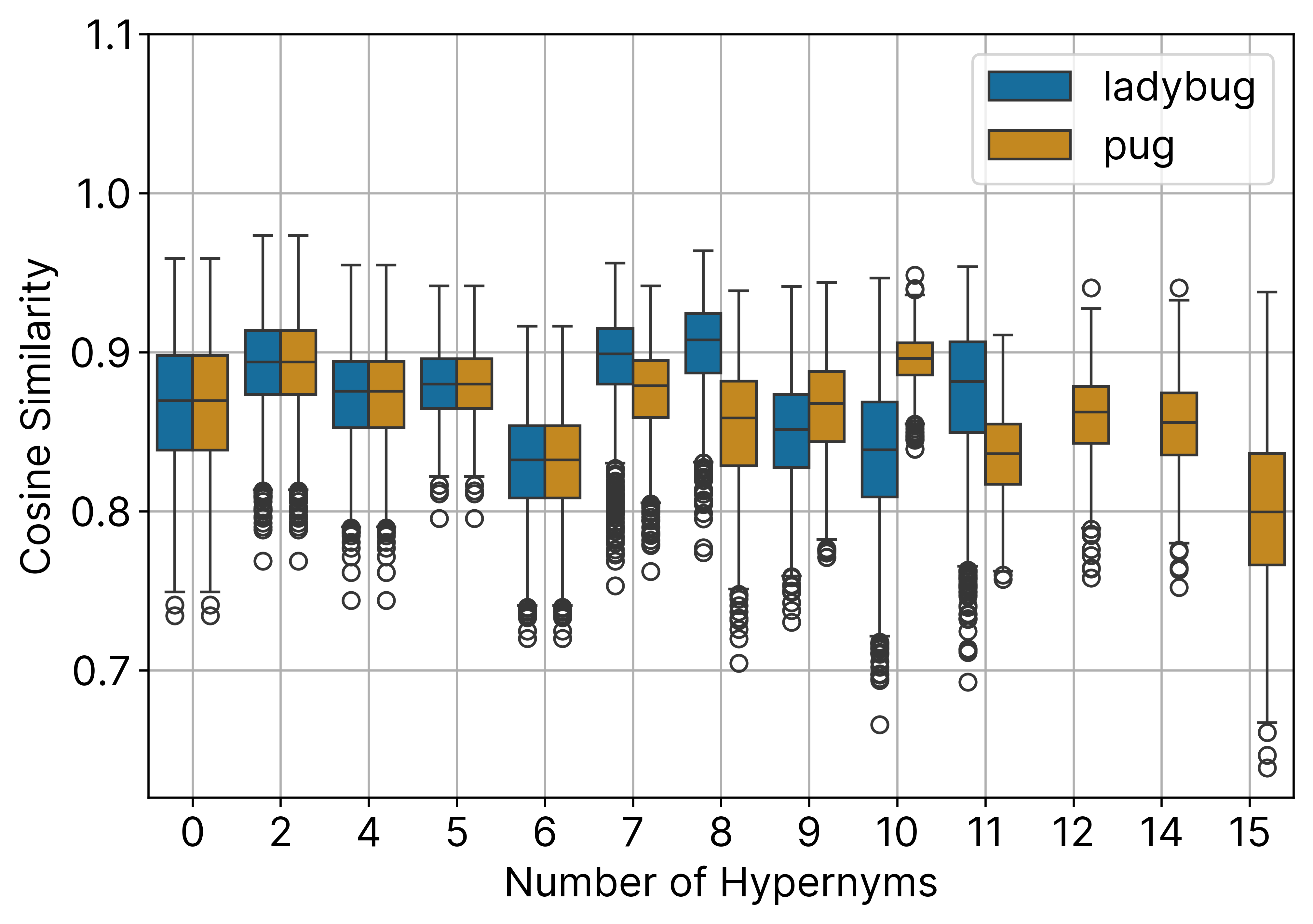
Figure 7: The figure demonstrates the independence of the concept broadness measured by the number of hypernyms as defined in WordNet [55] to the inter-image similarity of corresponding generated images.

In our experiment, we define the broadness of a concept based on the number of hypernyms in the WordNet hierarchy [55]. The more specific a concept the larger the number of hypernyms. We choose two ImageNet classes (“ladybug”, “pug”) and generate $50$ images for each concept as well as each hypernym of both concepts (with the most general concept being “entity”.) Then, we measure the cosine similarity of all images generated based on the same concept. The box plot of the cosine similarity across both concepts and all hypernyms, in Figure 7 indicates that we do not find a correlation. Thus, we hypothesize that the chosen temperature of the diffusion model has a stronger effect on image similarity than the broadness of the prompt used for image generation.

A.5 Intraclass Image Similarity

In addition to comparing natural and synthetic images as in Section 4.1, we also analyze the intraclass distance to compare the similarity among synthetic images. Intraclass distance refers to the degree of diversity or dissimilarity observed within a set of images of the same class. It quantifies how much the individual images deviate from the average or central tendency of the image set. In this context, intraclass distance is desirable, reflecting how visual concepts can appear in natural images. Higher similarity scores indicate greater divergence from natural occurrences of concepts.

Cosine similarity (CS) and “Euclidean distance” (ED) are commonly used metrics for measuring image similarity because they capture different aspects of similarity and complement each other. We compute the average CS and ED for each class and determine the overall class average. Table 5 provides a detailed overview of the results quantifying the similarity within synthetic images using CS and ED. When evaluating these results, it is important to note that high scores do not necessarily indicate optimal outcomes, as they suggest nearly identical images, which may lack intraclass distance. Conversely, very low scores imply significant differences among images, which might not capture the essence of the concept adequately. Ideally, we aim for somewhat similar yet slightly varied images representing the same class. The results show that the Stable Cascade (SC) model consistently achieves higher scores across all prompts compared to the Stable Diffusion XL 1.0-base (SDXL) model. Notably, it obtains the highest score for the two most elaborate prompts (4, 5). This indicates that the SC model tends to offer less intraclass distance in visually representing concepts.

Table 5: Intraclass Image Similarity. This table illustrates the impact of varying parameters within our CoSy framework. We evaluate 5 different prompts as input to 2 different text-to-image models. A random selection of 10 ImageNet classes is made, with each class name used as input to the prompt, denoted as [concept], resulting in 50 images generated per prompt using a text-to-image model. We compute the average intraclass similarity across all classes. Higher CS and lower ED values indicate greater similarity between the images. In intraclass image similarity, neither excessively high nor excessively low scores are desirable.

Prompt	Text-to-image	CS ($\uparrow$)	ED ($\downarrow$)
1. “a [concept]”	SDXL	0.83$\pm$0.07	5.85$\pm$1.41
	SC	0.92$\pm$0.03	4.03$\pm$1.00
2. “a painting of [concept]”	SDXL	0.87$\pm$0.05	4.94$\pm$1.13
	SC	0.92$\pm$0.03	3.95$\pm$0.88
3. “photo of [concept]”	SDXL	0.81$\pm$0.07	6.13$\pm$1.36
	SC	0.90$\pm$0.04	4.46$\pm$1.05
4. “realistic photo of [concept]”	SDXL	0.86$\pm$0.06	5.41$\pm$1.34
	SC	0.93$\pm$0.03	3.79$\pm$0.85
5. “realistic photo of a close up of [concept]”	SDXL	0.88$\pm$0.05	5.09$\pm$1.29
	SC	0.93$\pm$0.03	3.95$\pm$0.92

A.6 Model Stability

In this experiment, our goal is to evaluate the stability of the image generation method employed, aiming to ensure consistent results within our CoSy framework. We achieve this by varying the seed of the image generator and observing the impact on image generation. We anticipate consistent image representations across different model initializations, thus ensuring the stability of our framework.

For our analysis, we utilize ResNet18 and focus on its output neurons, as the ground-truth labels associated with these neurons are known. We randomly select six classes $s$ from the ImageNet validation dataset [39] and examine the corresponding $f_{i}$ class output neurons using CoSy. Here, we exclude the $s$ class from $\mathbb{A}_{0}$ and let $\mathbb{A}_{1}$ represent the $s$ class. To ensure robustness, we initialize the text-to-image model across a random set of 10 seeds. Our analysis involves calculating the first (mean) and second moment (STD) using $\Psi_{\text{AUC}}$, as well as evaluating the intraclass image similarity (refer to Section A.5) within each synthetic ground truth class.

The results for our experiment, as shown in Table 6, demonstrate remarkably high AUC scores, indicating near-perfect detection of synthetic ground truth classes across all image model initializations. Furthermore, the standard deviation is exceptionally low, suggesting consistent image generation regardless of the chosen seed. The intraclass similarity values indicate a certain degree of distance in the generated images, indicating high similarity yet distinctiveness. This intraclass distance is desirable, ensuring that the images are not identical but share common characteristics.

These findings underscore the reliability and consistency of our image generation pipeline within our CoSy framework. The high stability of text-to-image generation across different seeds and the diversity of image similarity contribute to the robustness of our approach.

Table 6: Model Stability. A comparison of various model initializations across 10 random seeds using SDXL.

Concept	AUC ($\uparrow$)	CS ($\uparrow$)	ED ($\downarrow$)
bulbul	0.9996$\pm$0.0002	0.91$\pm$0.03	3.99$\pm$0.66
china cabinet	0.9999$\pm$0.0001	0.89$\pm$0.04	5.00$\pm$0.90
leatherback turtle	0.9994$\pm$0.0001	0.91$\pm$0.04	4.65$\pm$0.87
beer bottle	0.9919$\pm$0.0038	0.80$\pm$0.08	6.79$\pm$1.41
half track	0.9998$\pm$0.0000	0.88$\pm$0.04	5.12$\pm$0.91
hard disc	1.0000$\pm$0.0001	0.90$\pm$0.05	4.64$\pm$1.17
Overall Mean	0.9984$\pm$0.0007	0.88$\pm$0.02	5.03$\pm$0.26

A.7 Prompt and Text-to-Image Model Comparison

Figure 8 showcases additional examples of synthetically generated images using both SDXL and SC across various prompts, highlighting the diversity and accuracy of concept representation.

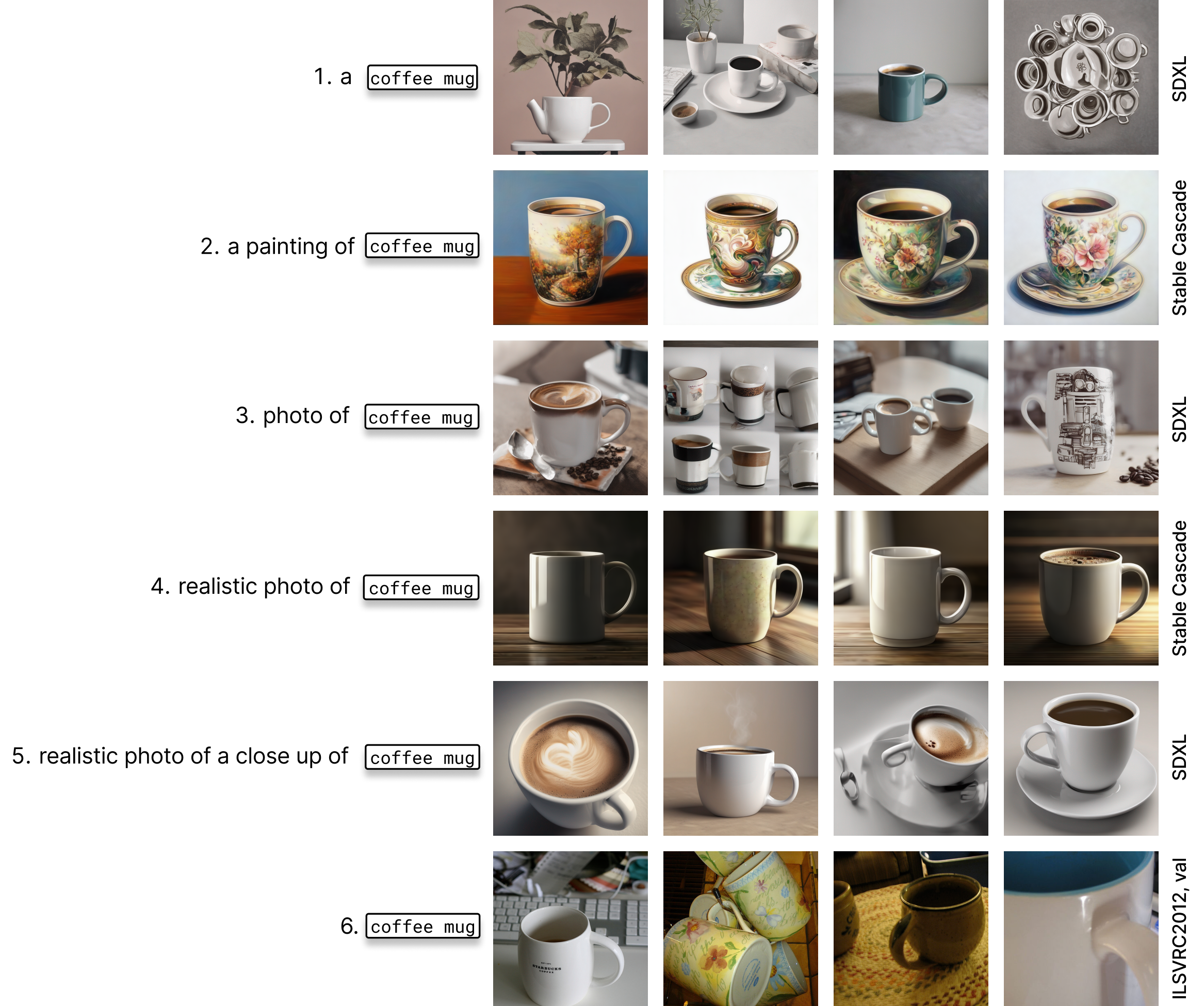
Figure 8: Example images for “coffee mug” generated by the text-to-image models SDXL and SC across various prompts. (1) and (3) present examples of synthetic images with relatively low intraclass similarity and relatively high natural-to-synthetic similarity scores. (2) shows examples of synthetic images with the lowest similarity to natural images. (4) illustrates examples of synthetic images with the highest similarity to other synthetic images within the same class. (5) showcases examples of synthetic images with the highest similarity to natural images. (6) displays examples of natural images from the ImageNet validation dataset [39] belonging to the class “coffee mug”.

References

- [1] Wojciech Samek and Klaus-Robert Müller “Towards explainable artificial intelligence” In Explainable AI: interpreting, explaining and visualizing deep learning Springer, 2019, pp. 5–22
- [2] Feiyu Xu et al. “Explainable AI: A brief survey on history, research areas, approaches and challenges” In Natural Language Processing and Chinese Computing: 8th CCF International Conference, NLPCC 2019, Dunhuang, China, October 9–14, 2019, Proceedings, Part II 8, 2019, pp. 563–574 Springer
- [3] Sebastian Bach et al. “On pixel-wise explanations for non-linear classifier decisions by layer-wise relevance propagation” In PloS one 10.7 Public Library of Science San Francisco, CA USA, 2015, pp. e0130140
- [4] K Simonyan, A Vedaldi and A Zisserman “Deep inside convolutional networks: visualising image classification models and saliency maps” In Proceedings of the International Conference on Learning Representations (ICLR), 2014 ICLR
- [5] Ramprasaath R Selvaraju et al. “Grad-cam: Visual explanations from deep networks via gradient-based localization” In Proceedings of the IEEE international conference on computer vision, 2017, pp. 618–626
- [6] Daniel Smilkov et al. “Smoothgrad: removing noise by adding noise” In arXiv preprint arXiv:1706.03825, 2017
- [7] Chris Olah et al. “Zoom in: An introduction to circuits” In Distill 5.3, 2020, pp. e00024–001
- [8] Kevin Ro Wang et al. “Interpretability in the Wild: a Circuit for Indirect Object Identification in GPT-2 Small” In The Eleventh International Conference on Learning Representations, 2022
- [9] Steven Bills et al. “Language models can explain neurons in language models”, https://openaipublic.blob.core.windows.net/neuron-explainer/paper/index.html, 2023
- [10] Neel Nanda et al. “Progress measures for grokking via mechanistic interpretability” In The Eleventh International Conference on Learning Representations, 2022
- [11] David Bau et al. “Network Dissection: Quantifying Interpretability of Deep Visual Representations” In Proceedings of the IEEE Conference on Computer Vision and Pattern Recognition (CVPR), 2017
- [12] Jesse Mu and Jacob Andreas “Compositional Explanations of Neurons” In Advances in Neural Information Processing Systems 33 Curran Associates, Inc., 2020, pp. 17153–17163 URL: https://proceedings.neurips.cc/paper_files/paper/2020/file/c74956ffb38ba48ed6ce977af6727275-Paper.pdf
- [13] Evan Hernandez et al. “Natural Language Descriptions of Deep Features” In International Conference on Learning Representations, 2022 URL: https://openreview.net/forum?id=NudBMY-tzDr
- [14] Neha Kalibhat et al. “Identifying Interpretable Subspaces in Image Representations” In Proceedings of the 40th International Conference on Machine Learning 202, Proceedings of Machine Learning Research PMLR, 2023, pp. 15623–15638 URL: https://proceedings.mlr.press/v202/kalibhat23a.html
- [15] Tuomas Oikarinen and Tsui-Wei Weng “CLIP-Dissect: Automatic Description of Neuron Representations in Deep Vision Networks” In International Conference on Learning Representations, 2023
- [16] Kirill Bykov et al. “Labeling Neural Representations with Inverse Recognition” In Thirty-seventh Conference on Neural Information Processing Systems, 2023
- [17] Dumitru Erhan, Yoshua Bengio, Aaron Courville and Pascal Vincent “Visualizing higher-layer features of a deep network” In University of Montreal 1341.3, 2009, pp. 1
- [18] Chris Olah, Alexander Mordvintsev and Ludwig Schubert “Feature visualization” In Distill 2.11, 2017, pp. e7
- [19] Anh Nguyen et al. “Synthesizing the preferred inputs for neurons in neural networks via deep generator networks” In Advances in neural information processing systems 29, 2016
- [20] Thomas Fel et al. “Unlocking Feature Visualization for Deep Network with MAgnitude Constrained Optimization” In Thirty-seventh Conference on Neural Information Processing Systems, 2023 URL: https://openreview.net/forum?id=J7VoDuzuKs
- [21] Judy Borowski et al. “Natural images are more informative for interpreting cnn activations than state-of-the-art synthetic feature visualizations” In NeurIPS 2020 Workshop SVRHM, 2020
- [22] Gabriel Goh et al. “Multimodal neurons in artificial neural networks” In Distill 6.3, 2021, pp. e30
- [23] Naoya Yoshimura, Takuya Maekawa and Takahiro Hara “Toward understanding acceleration-based activity recognition neural networks with activation maximization” In 2021 International Joint Conference on Neural Networks (IJCNN), 2021, pp. 1–8 IEEE
- [24] Dennis Grinwald, Kirill Bykov, Shinichi Nakajima and Marina MC Höhne “Visualizing the Diversity of Representations Learned by Bayesian Neural Networks” In Transactions on Machine Learning Research, 2023
- [25] Stephen Casper et al. “Red teaming deep neural networks with feature synthesis tools” In Thirty-seventh Conference on Neural Information Processing Systems, 2023
- [26] Kirill Bykov et al. “DORA: Exploring Outlier Representations in Deep Neural Networks” In Transactions on Machine Learning Research, 2023
- [27] Dilyara Bareeva et al. “Manipulating Feature Visualizations with Gradient Slingshots” In arXiv preprint arXiv:2401.06122, 2024
- [28] Robert Geirhos et al. “Don’t trust your eyes: on the (un) reliability of feature visualizations” In arXiv preprint arXiv:2306.04719, 2023
- [29] Jonathan Marty, Eugene Belilovsky and Michael Eickenberg “Adversarial Attacks on Feature Visualization Methods” In NeurIPS ML Safety Workshop, 2022 URL: https://openreview.net/forum?id=J51K0rszIjr
- [30] Alec Radford et al. “Learning transferable visual models from natural language supervision” In International conference on machine learning, 2021, pp. 8748–8763 PMLR
- [31] Chirag Agarwal et al. “OpenXAI: Towards a Transparent Evaluation of Model Explanations” In Thirty-sixth Conference on Neural Information Processing Systems Datasets and Benchmarks Track, 2022 URL: https://openreview.net/forum?id=MU2495w47rz
- [32] Anna Hedström et al. “Quantus: An Explainable AI Toolkit for Responsible Evaluation of Neural Network Explanations and Beyond” In Journal of Machine Learning Research 24.34, 2023, pp. 1–11
- [33] Anna Hedström, Leander Weber, Sebastian Lapuschkin and Marina Höhne “Sanity Checks Revisited: An Exploration to Repair the Model Parameter Randomisation Test” In XAI in Action: Past, Present, and Future Applications, 2023 URL: https://openreview.net/forum?id=vVpefYmnsG
- [34] Tianyi Zhang et al. “BERTScore: Evaluating Text Generation with BERT” In International Conference on Learning Representations, 2019
- [35] Mert Yuksekgonul, Maggie Wang and James Zou “Post-hoc Concept Bottleneck Models” In The Eleventh International Conference on Learning Representations, 2022
- [36] Anna Hedström et al. “The Meta-Evaluation Problem in Explainable AI: Identifying Reliable Estimators with MetaQuantus” arXiv, 2023 DOI: 10.48550/ARXIV.2302.07265
- [37] Dustin Podell et al. “SDXL: Improving Latent Diffusion Models for High-Resolution Image Synthesis” In The Twelfth International Conference on Learning Representations, 2023
- [38] Pablo Pernias et al. “Würstchen: An Efficient Architecture for Large-Scale Text-to-Image Diffusion Models” In The Twelfth International Conference on Learning Representations, 2023
- [39] Olga Russakovsky et al. “ImageNet Large Scale Visual Recognition Challenge” In International Journal of Computer Vision (IJCV) 115.3, 2015, pp. 211–252 DOI: 10.1007/s11263-015-0816-y
- [40] Kaiming He, Xiangyu Zhang, Shaoqing Ren and Jian Sun “Deep residual learning for image recognition” In Proceedings of the IEEE conference on computer vision and pattern recognition, 2016, pp. 770–778
- [41] Gao Huang, Zhuang Liu, Laurens Van Der Maaten and Kilian Q Weinberger “Densely connected convolutional networks” In Proceedings of the IEEE conference on computer vision and pattern recognition, 2017, pp. 4700–4708
- [42] Christian Szegedy et al. “Going deeper with convolutions” In Proceedings of the IEEE conference on computer vision and pattern recognition, 2015, pp. 1–9
- [43] Alexey Dosovitskiy et al. “An Image is Worth 16x16 Words: Transformers for Image Recognition at Scale” In International Conference on Learning Representations, 2020
- [44] Bolei Zhou et al. “Places: A 10 million Image Database for Scene Recognition” In IEEE Transactions on Pattern Analysis and Machine Intelligence IEEE, 2017
- [45] Yann LeCun, Yoshua Bengio and Geoffrey Hinton “Deep learning” In nature 521.7553 Nature Publishing Group UK London, 2015, pp. 436–444
- [46] David Cheng-Han Chiang and Hung-yi Lee “A Closer Look into Using Large Language Models for Automatic Evaluation” In Findings of the Association for Computational Linguistics: EMNLP 2023, Singapore, December 6-10, 2023 Association for Computational Linguistics, 2023, pp. 8928–8942
- [47] Satyapriya Krishna et al. “Post Hoc Explanations of Language Models Can Improve Language Models” In Thirty-seventh Conference on Neural Information Processing Systems, 2023 URL: https://openreview.net/forum?id=3H37XciUEv
- [48] Nicholas Kroeger et al. “Are Large Language Models Post Hoc Explainers?” In CoRR abs/2310.05797, 2023
- [49] Christoph Molnar “Interpretable Machine Learning”, 2022 URL: https://christophm.github.io/interpretable-ml-book
- [50] Kelvin Xu et al. “Show, attend and tell: Neural image caption generation with visual attention” In International conference on machine learning, 2015, pp. 2048–2057 PMLR
- [51] Thomas H Cormen, Charles E Leiserson, Ronald L Rivest and Clifford Stein “Introduction to algorithms” MIT press, 2022
- [52] Sepp Hochreiter and Jürgen Schmidhuber “Long short-term memory” In Neural computation 9.8 MIT press, 1997, pp. 1735–1780
- [53] Christoph Schuhmann et al. “LAION-400M: Open Dataset of CLIP-Filtered 400 Million Image-Text Pairs” In NeurIPS Workshop Datacentric AI, online (online), 14 Dec 2021 - 14 Dec 2021, 2021, pp. 5 p. URL: https://juser.fz-juelich.de/record/905696
- [54] Tuomas Oikarinen and Tsui-Wei Weng “CLIP-Dissect: Automatic Description of Neuron Representations in Deep Vision Networks” In The Eleventh International Conference on Learning Representations, 2022
- [55] George A Miller “WordNet: a lexical database for English” In Communications of the ACM 38.11 ACM New York, NY, USA, 1995, pp. 39–41