Did Binary Neutron Star Merger GW170817 Leave Behind A Long-lived Neutron Star?
Abstract
We consider the observational implications of the binary neutron star (BNS) merger GW170817 leaving behind a rapidly rotating massive neutron star that launches a relativistic, equatorial outflow as well as a jet. We show that if the equatorial outflow (ring) is highly beamed in the equatorial plane, its luminosity can be “hidden” from view until late times, even if carrying a significant fraction of the spin-down energy of the merger remnant. This hidden ring reveals itself as a re-brightening in the light curve once it slows down enough for Earth to be within the ring’s relativistic beaming solid angle. We compute semi-analytic light curves using this model and find they are in agreement with the observations thus far, and we provide predictions for the ensuing afterglow.
1 Introduction
The historic gravitational wave (GW) event, GW170817 (Abbott et al., 2017), heightened interest in the coalescence of neutron stars (NSs) even outside of the field of astrophysics due to the array of fundamental physical questions that arise from the catastrophic merger (see e.g., Metzger, 2017; Lattimer, 2021, for comprehensive reviews). A bright electromagnetic (EM) counterpart of GW170817 was a gamma-ray burst (GRB; GRB 170817A; Abbott et al., 2017), solidifying the identification of the GW signal as that of a binary neutron star (BNS) merger. The GRB 170817A afterglow shows evidence for a structured aspherical outflow (Sari et al., 1999; Granot, 2005; DuPont et al., 2023) — which was followed by a rise in X-ray flux at the time of writing (see Margutti et al., 2017; Troja et al., 2019, 2020, 2022; Hajela et al., 2022, for a compilation of GRB 170817A observations).
Prevailing theories that explain the GW plus EM signal of GW170817 involve the BNS merger forming a short-lived remnant that eventually collapses into a black hole (BH) surrounded by an accretion disk that powers a GRB jet (Murguia-Berthier et al., 2014; Lawrence et al., 2015). The BH collapse is turned to as a reason to explain the production of a GRB as well as the observed lack of the of the merger remnant’s rotational energy deposited into the BNS ejecta cloud (Margalit & Metzger, 2017).
In this Letter, we revisit the question of whether GW170817 may have left behind a long-lived massive NS remnant. We consider the case that the BNS merger creates a stable or quasi-stable massive NS that rapidly rotates to the point of centrifugally slinging matter into a ultra-relativistic equatorial outflow (see e.g., Thompson, 2005, 2007)111Here, “rapid rotation” means a spin period of .. If the equatorial outflow is ultra-relativistic, then a sizable fraction of the NS rotational energy can be beamed into the equatorial plane. As the equatorial outflow burrows through the merger ejecta, the rapidly rotating proto-NS could (i) generate a magnetic tower that stretches along the rotation axis, thus powering a GRB jet (e.g., Uzdensky & MacFadyen, 2006, 2007) and/or (ii) undergo an eventual collapse into a BH, but on a longer timescale than previously thought.
We present the theoretical light curves of a jet-ring model in comparison with the observed data and show that late time observations can be helpful for constraining the equation of state of dense matter (e.g., Tews et al., 2018).
This Letter is organized as follows: Section 2 discusses the theoretical setup and dynamics of the relativistic ring produced by magneto-centrifugal slinging, Section 3 discusses our results in comparing our model with current observations, and Section 4 discusses our conclusions and relevance of this work.
2 Relativistic Ring Dynamics and Emission
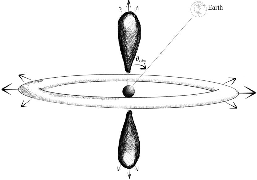
For illustrative purposes, we use simple arguments and assumptions to derive the dynamics of a relativistic ring expelled from a magnetic rotator either through magneto-centrifugal slinging or magnetic dissipation by the equatorial current sheet. If the relativistic ring overcomes the magnetic hoop stress, it breaks out of the BNS ejecta cloud and propagates into the interstellar medium (ISM) where it will eventually sweep up mass comparable to its own and gradually open its beaming cone until visible from Earth. The BNS ejecta is assumed to produce a collimated outflow along the rotation axis, i.e., a magnetic tower. The scenario of this structured jet-ring BNS model is illustrated in Figure 1.
2.1 Toroidal outflow from a BNS merger
The magnetic rotator’s spin energy is radiated away at the rate
| (1) |
where is the rotational energy, is the magnetic rotator mass, is the moment of inertia, is the rotation frequency, is the speed of light, is the magnetic moment, and a dot over a variable signifies differentiation with respect to time. The rightmost equality in Equation (1) is the standard magnetic dipole radiation formula. From Equation (1), the rotation frequency evolves as
| (2) |
where is the rotation frequency of the nascent magnetic rotator, and is the spin-down time. We now set for the remainder of our derivations. Let us assume that outside of the light cylinder some fraction, , of the rotational energy is beamed into an expanding relativistic ring with energy , where is the initial half-opening angle of the ring’s core, is the proper mass density, is the specific enthalpy, is the adiabatic index, is the pressure, is the Lorentz factor, and is the bulk velocity in units of . This ring will interact with a toroidal magnetic field of strength that grows linearly with time (Uzdensky & MacFadyen, 2007). If the ring is a hot relativistic fluid with adiabatic index , then its pressure dominates over the rest mass energy density such that . Roughly, for this relativistic ring to overcome the magnetic field hoop stress and break out of the ejecta cloud, we require where is the lab frame number density, is the proton mass, is the initial magnetization, is the light crossing time across the expanding ejecta cloud, is the initial radius of the ejecta cloud, and is the velocity of the ejecta cloud, assumed to be non-relativistic. This condition leads to an upper bound on the “break out” Lorentz factor of the ring,
| (3) |
where we’ve neglected numerical constant terms and is the energy per baryon222 is related to , the initial random Lorentz factor or the dimensionless entropy as it’s often called in other texts.. Conversely, if the ring is halted by the magnetic hoop stress it becomes baryon loaded as plasma accumulates. Eventually the rest mass energy of the ring dominates over the pressure such that . These conditions might cause the ring to be redirected into a magnetic tower (e.g., Uzdensky & MacFadyen, 2007; Bucciantini et al., 2012). Immediately, one finds from Equation (3) that for a slow-moving cavity () and at early times (), the breakout Lorentz factor is dominated by the ratio which appears to be the limiting factor that governs a successful ring breakout. Note that Equation (3) is an estimate and will need a direct numerical special relativistic magneto-hydrodynamics simulation to confirm its validity.
2.2 Dynamics of lateral spreading
We now consider that the relativistic ring breaks out from the BNS merger ejecta cloud and travels far into the ISM where it will eventually sweep up mass comparable to its own and begin to decelerate. At the onset of this declaration phase, we compute the dynamics of the expanding relativistic ring as it begins to spread sideways.
The energy in the blast wave is approximately
| (4) |
where is four-velocity, is the ambient density and is taken to obey where is the mass-loading parameter, and is the blast wave solid angle.
For simplicity, we assume the solid angle of the blast wave is constant with respect to such that , unlike the more careful “trumpet” model computed by Rhoads (1999). From energy conservation, we can write
| (5) |
Since , the evolution of the bulk flow goes as
| (6) |
The sideways spreading of the perpendicular arc length of the blast wave333Taken from the point of view of a parcel at the very edge of the shock arc., , can be evaluated as
| (7) |
where is the velocity at which the shock arc opens up, is the infinitesimal proper time, and is the velocity parallel to the bulk flow and can be taken as . By noting that the proper time transforms into the lab frame time as and writing , it follows that , allowing us to write Equation (6) as
| (8) |
By solving for the combination , the above equation becomes separable and takes the form
| (9) |
Letting , taking with being the half-opening angle of the ring at time , and assuming , we arrive at
| (10) |
Equation (10) poses a distinction from the jet case in that it shows algebraic spreading of the ring-like blast wave instead of exponential or logarithmic spreading of jets (Granot & Piran, 2012; Duffell & Laskar, 2018).
2.3 Semi-analytic light curves
The light curves are computed using the afterglowpy code (Ryan et al., 2020), which assumes synchrotron radiation as the dominant emission mechanism. At its core, afterglowpy solves
| (11) |
where is the redshift, is the luminosity distance, is the Doppler factor, is the unit vector pointing from the observer to the source, and is the source frame emissivity. The details of the numerical scheme are explained in Ryan et al. (2020) and therefore will not be discussed here. Instead, we list off the important parameters and their definitions in Table 1. For the structured jet, we use the GaussianCore blast wave model provided by afterglowpy out of the box, and we use the GW170817 parameters given in Ryan et al. (2020) to fit the structured jet to the early observations. To arrive at a structured ring configuration, we assume a Gaussian energy profile of the form:
| (12) |
where and is approximated as
| (13) |
The maximal rotational energy of very massive NSs can approach (Metzger et al., 2015), so we use that energy as an upper bound. The fraction, , is a free parameter and for comparison, we explore the respective afterglows from structured rings with values and . We also note that we added the Equation (10) spreading prescription to the afterglowpy code to dynamically capture the off-plane afterglow rise of the toroidal outflow. We use the FlatLambdaCDM class in astropy (Astropy Collaboration et al., 2013, 2018, 2022) version 6.0.0, assuming a flat CDM cosmology with and to convert redshift into luminosity distance. We set and is calculated based on Equation 9 in Ryan et al. (2020). The light curve parameters are highly degenerate, but we fix based on upper limits inferred by Hajela et al. (2019) and based on constraints provided by observations (Mooley et al., 2018; Finstad et al., 2018; Hotokezaka et al., 2019; Ghirlanda et al., 2019). The data products we use were made available to us by the first author of Hajela et al. (2022). This concludes the ingredients needed for the analysis.
| Parameter | Definition |
|---|---|
| Isotropic-equivalent energy | |
| Observer angle with respect to polar axis | |
| Initial opening angle of blast wave | |
| Number density of protons | |
| Fraction of electrons accelerated | |
| Redshift | |
| Electron fraction of energy density | |
| Magnetic field fraction of energy density | |
| Electron energy distribution index |
3 Results
The results of our two-component model fitted to the GRB 170817A afterglow data are shown in Figures 2 and 3. The radio data were observed using the Karl G. Jansky Very Large Array (VLA; Condon et al., 1998) at 3 GHz, and the X-ray data were from the Chandra X-ray Observatory (CXO; Weisskopf et al., 2000a)444We manually converted the unabsorbed X-ray flux in Table 1 of Hajela et al. (2022) to units of milli-Jansky (mJy) given the information in that table..
Figure 2 showcases the standard structured jet (black dash-dotted curve) in conjunction with our structured ring (black dashed curve) afterglow hypothesis. In this comparison, we model the ring that has or 10% of the magnetic rotator’s rotational energy. When summed, the jet-ring model shows a decent fit with the GRB 170817A afterglow data at the time of writing. We also plot an array of hypothetical relativistic rings (purple dashed curves) with various opening angles in the range to constrain the geometry of the outflow needed to still fit the observations555The range of opening angles also produced a range of based on Equation 13.. Note that the parameters in Figure 2 are not statistically relaxed, but are only meant to demonstrate how a highly beamed, off-plane, ring-like geometry can reasonably fit the late-time observations.
As an extreme case, we also plot in Figure 3 the structured ring light curves if all of the rotational energy was focused into the magnetic rotator’s equatorial plane (i.e., .) Under these conditions, we find that the physical parameters of the system need not change much from the previously calculated structured ring aside from varying and to within a few percent of their previous values and increasing the angular size of the ring from to . The ring’s peak brightness is almost on par with the jet’s peak brightness even after 1000 days. This is due to the ring’s slower spreading dynamics coupled with its energy content being larger than the jet’s by a factor . We again plot as purple dashed curves. Again, the parameters in Figure 3 are not statistically relaxed, but are simply used as representative configurations of the ideal structured ring outflows that can still fit the observations given that all of the spin-down energy of the magnetic rotator is beamed in the equatorial plane.
Equally important, although the parameters in Table 1 are highly degenerate, we could not find structured ring afterglows that could fit the early phase of the light curve evolution for GRB 170817A. That is to say, we find that the observations preceding the re-brightening in the afterglow light curves from GRB 170817A must come from a structured jet-like outflow geometry due to the early decay phase being too steep to be explained by any ring-like geometry no matter what combination of parameters we use from Table 1.
4 Discussion
In this work, we calculate theoretical light curves of a jet-ring structure formed just after a binary neutron star (BNS) merger. We compare this model with the observed data from the GW170817 BNS merger event, and find that if the equatorial ring is highly beamed away from the line of sight, then its energy can be hidden until days, which might explain the late-time excess emission observed in the afterglow (Margutti et al., 2017; Troja et al., 2019, 2020, 2022; Hajela et al., 2022). The off-axis gamma-ray burst (GRB) jet is seen first before its afterglow begins decaying, wherein the ring’s emission shines through once the ring outflow slows down enough for Earth to be inside of its beaming cone. This effect emerges as a re-brightening at late times ( days) in the afterglow. This emission differs from previous calculations of later-time ( days) bumps due to the slower dynamical ejecta of NS mergers (e.g., Hotokezaka et al., 2018).
Based on these results, we ask whether GW170817 may have left behind a NS as opposed to collapsing into a black hole (BH). The NS collapse is usually invoked to explain the lack of rotational energy that would be deposited into the merger ejecta (Metzger et al., 2015; Margalit & Metzger, 2017), but we consider that instead the rapidly rotating remnant beams a significant fraction of this rotational energy in the equatorial plane, and we at Earth miss the initial beamed emission and instead see the opening phase of the equatorial outflow as it decelerates. This might imply that the upper bound mass limits are higher than those previously computed for GW170817 (Margalit & Metzger, 2017; Shibata et al., 2017; Ruiz et al., 2018; Rezzolla et al., 2018; Shibata et al., 2019) while still falling into absolute limits set by nuclear physics (Gandolfi et al., 2012).
Our model is idealized in that we assume a significant fraction of the energy flux is focused into the equator where we remain agnostic about the focusing mechanism. We also do not know how long this focusing effect will last as the BNS ejecta cloud propagates outward. We compare a weakly beamed ring () and a highly beamed ring () and find that both configurations can fit the observations reasonable well, but each of these beaming modes imply a different fate for the NS. For example, if only 10% of the rotational energy is beamed in the equatorial plane, then the NS must eventually collapse into a BH as to not violate the electromagnetic constraints of the kilonova (KN) ejecta from GW170817 (Metzger, 2017). On the other hand, if almost all of the rotational energy is in fact beamed into the equatorial plane, then it opens up the possibility that the remnant remains a stable NS given a stiff enough NS equation of state and/or the total mass of the binary is low (Shibata & Taniguchi, 2006).
Still, it is admittedly difficult to reconcile the fact that with the Kelvin-Helmholtz timescale being , the hypothetically stable NS will now be cold and the stability of hot remnants transitioning to cold slow / non- rotators is still poorly understood. In the previous estimate, is the dimensionless total binary mass (Abbott et al., 2019), is the dimensionless neutrino luminosity (Thompson et al., 2004), and is the dimensionless radius of the proto-NS inferred from general relativistic simulations (Sekiguchi et al., 2016). While some calculations used GW170817 to weakly constrain the maximum mass of cold NSs to (e.g, Shibata et al., 2019), we suggest that observations of the late-time light curve morphology might shift these upper limits towards higher values with the most extreme case being that GW170817 left behind a remnant. At the most basic level, given what fraction of the magnetic rotator’s energy can be feasibly hidden due to beaming in the equatorial plane such that the magnetic rotator never has to collapse into a BH to satisfy any EM constraints, our model could have significant implications on the equation of state of dense matter.
In order to compute the structure of equatorial outflows from BNS remnants we plan to perform 3D relativistic magneto-hydrodynamics simulations of a rapid magnetized rotator embedded in a BNS ejecta cloud. Previous simulations in 2D axisymmetry have shown that this sort of configuration collimates almost all of the equatorial outflow into polar jet-like outflow and therefore possesses no relativistic toroidal component (e.g., Bucciantini et al., 2007, 2008, 2012). However, the polar focusing seen in previous works may not be a universal solution given that this focusing effect may be an artifact of the imposed axisymmetry (see e.g., Porth et al., 2014). Furthermore, a jet-ring structure is seen in observations of the Crab pulsar (Hester et al., 1995, 2002; Weisskopf et al., 2000b), and we remain curious as to whether the canonical BNS merger event can produce a stable remnant with Crab-like morphology given that the relativistic ring successfully carries away a significant amount of the rotational energy.
References
- Abbott et al. (2017) Abbott, B. P., Abbott, R., Abbott, T. D., et al. 2017, Phys. Rev. Lett., 119, 161101, doi: 10.1103/PhysRevLett.119.161101
- Abbott et al. (2019) —. 2019, Physical Review X, 9, 011001, doi: 10.1103/PhysRevX.9.011001
- Astropy Collaboration et al. (2013) Astropy Collaboration, Robitaille, T. P., Tollerud, E. J., et al. 2013, A&A, 558, A33, doi: 10.1051/0004-6361/201322068
- Astropy Collaboration et al. (2018) Astropy Collaboration, Price-Whelan, A. M., Sipőcz, B. M., et al. 2018, AJ, 156, 123, doi: 10.3847/1538-3881/aabc4f
- Astropy Collaboration et al. (2022) Astropy Collaboration, Price-Whelan, A. M., Lim, P. L., et al. 2022, ApJ, 935, 167, doi: 10.3847/1538-4357/ac7c74
- Bucciantini et al. (2012) Bucciantini, N., Metzger, B. D., Thompson, T. A., & Quataert, E. 2012, MNRAS, 419, 1537, doi: 10.1111/j.1365-2966.2011.19810.x
- Bucciantini et al. (2007) Bucciantini, N., Quataert, E., Arons, J., Metzger, B. D., & Thompson, T. A. 2007, MNRAS, 380, 1541, doi: 10.1111/j.1365-2966.2007.12164.x
- Bucciantini et al. (2008) —. 2008, MNRAS, 383, L25, doi: 10.1111/j.1745-3933.2007.00403.x
- Condon et al. (1998) Condon, J. J., Cotton, W. D., Greisen, E. W., et al. 1998, AJ, 115, 1693, doi: 10.1086/300337
- Duffell & Laskar (2018) Duffell, P. C., & Laskar, T. 2018, ApJ, 865, 94, doi: 10.3847/1538-4357/aadb9c
- DuPont et al. (2023) DuPont, M., MacFadyen, A., & Sari, R. 2023, ApJ, 957, 29, doi: 10.3847/1538-4357/acffbc
- Finstad et al. (2018) Finstad, D., De, S., Brown, D. A., Berger, E., & Biwer, C. M. 2018, ApJ, 860, L2, doi: 10.3847/2041-8213/aac6c1
- Gandolfi et al. (2012) Gandolfi, S., Carlson, J., & Reddy, S. 2012, Phys. Rev. C, 85, 032801, doi: 10.1103/PhysRevC.85.032801
- Ghirlanda et al. (2019) Ghirlanda, G., Salafia, O. S., Paragi, Z., et al. 2019, Science, 363, 968, doi: 10.1126/science.aau8815
- Granot (2005) Granot, J. 2005, ApJ, 631, 1022, doi: 10.1086/432676
- Granot & Piran (2012) Granot, J., & Piran, T. 2012, MNRAS, 421, 570, doi: 10.1111/j.1365-2966.2011.20335.x
- Hajela et al. (2019) Hajela, A., Margutti, R., Alexander, K. D., et al. 2019, ApJ, 886, L17, doi: 10.3847/2041-8213/ab5226
- Hajela et al. (2022) Hajela, A., Margutti, R., Bright, J. S., et al. 2022, ApJ, 927, L17, doi: 10.3847/2041-8213/ac504a
- Hester et al. (1995) Hester, J. J., Scowen, P. A., Sankrit, R., et al. 1995, ApJ, 448, 240, doi: 10.1086/175956
- Hester et al. (2002) Hester, J. J., Mori, K., Burrows, D., et al. 2002, ApJ, 577, L49, doi: 10.1086/344132
- Hotokezaka et al. (2018) Hotokezaka, K., Kiuchi, K., Shibata, M., Nakar, E., & Piran, T. 2018, ApJ, 867, 95, doi: 10.3847/1538-4357/aadf92
- Hotokezaka et al. (2019) Hotokezaka, K., Nakar, E., Gottlieb, O., et al. 2019, Nature Astronomy, 3, 940, doi: 10.1038/s41550-019-0820-1
- Lattimer (2021) Lattimer, J. M. 2021, Annual Review of Nuclear and Particle Science, 71, 433, doi: 10.1146/annurev-nucl-102419-124827
- Lawrence et al. (2015) Lawrence, S., Tervala, J. G., Bedaque, P. F., & Miller, M. C. 2015, ApJ, 808, 186, doi: 10.1088/0004-637X/808/2/186
- Margalit & Metzger (2017) Margalit, B., & Metzger, B. D. 2017, ApJ, 850, L19, doi: 10.3847/2041-8213/aa991c
- Margutti et al. (2017) Margutti, R., Berger, E., Fong, W., et al. 2017, ApJ, 848, L20, doi: 10.3847/2041-8213/aa9057
- Metzger (2017) Metzger, B. D. 2017, Living Reviews in Relativity, 20, 3, doi: 10.1007/s41114-017-0006-z
- Metzger et al. (2015) Metzger, B. D., Margalit, B., Kasen, D., & Quataert, E. 2015, MNRAS, 454, 3311, doi: 10.1093/mnras/stv2224
- Mooley et al. (2018) Mooley, K. P., Deller, A. T., Gottlieb, O., et al. 2018, Nature, 561, 355, doi: 10.1038/s41586-018-0486-3
- Murguia-Berthier et al. (2014) Murguia-Berthier, A., Montes, G., Ramirez-Ruiz, E., De Colle, F., & Lee, W. H. 2014, ApJ, 788, L8, doi: 10.1088/2041-8205/788/1/L8
- Porth et al. (2014) Porth, O., Komissarov, S. S., & Keppens, R. 2014, MNRAS, 438, 278, doi: 10.1093/mnras/stt2176
- Rezzolla et al. (2018) Rezzolla, L., Most, E. R., & Weih, L. R. 2018, ApJ, 852, L25, doi: 10.3847/2041-8213/aaa401
- Rhoads (1999) Rhoads, J. E. 1999, ApJ, 525, 737, doi: 10.1086/307907
- Ruiz et al. (2018) Ruiz, M., Shapiro, S. L., & Tsokaros, A. 2018, Phys. Rev. D, 97, 021501, doi: 10.1103/PhysRevD.97.021501
- Ryan et al. (2020) Ryan, G., van Eerten, H., Piro, L., & Troja, E. 2020, ApJ, 896, 166, doi: 10.3847/1538-4357/ab93cf
- Sari et al. (1999) Sari, R., Piran, T., & Halpern, J. P. 1999, ApJ, 519, L17, doi: 10.1086/312109
- Sekiguchi et al. (2016) Sekiguchi, Y., Kiuchi, K., Kyutoku, K., Shibata, M., & Taniguchi, K. 2016, Phys. Rev. D, 93, 124046, doi: 10.1103/PhysRevD.93.124046
- Shibata et al. (2017) Shibata, M., Fujibayashi, S., Hotokezaka, K., et al. 2017, Phys. Rev. D, 96, 123012, doi: 10.1103/PhysRevD.96.123012
- Shibata & Taniguchi (2006) Shibata, M., & Taniguchi, K. 2006, Phys. Rev. D, 73, 064027, doi: 10.1103/PhysRevD.73.064027
- Shibata et al. (2019) Shibata, M., Zhou, E., Kiuchi, K., & Fujibayashi, S. 2019, Phys. Rev. D, 100, 023015, doi: 10.1103/PhysRevD.100.023015
- Tews et al. (2018) Tews, I., Margueron, J., & Reddy, S. 2018, Phys. Rev. C, 98, 045804, doi: 10.1103/PhysRevC.98.045804
- Thompson (2005) Thompson, T. A. 2005, Nuovo Cimento C Geophysics Space Physics C, 28, 583, doi: 10.1393/ncc/i2005-10109-2
- Thompson (2007) Thompson, T. A. 2007, in Revista Mexicana de Astronomia y Astrofisica Conference Series, Vol. 27, Revista Mexicana de Astronomia y Astrofisica, vol. 27, 80–90, doi: 10.48550/arXiv.astro-ph/0611368
- Thompson et al. (2004) Thompson, T. A., Chang, P., & Quataert, E. 2004, ApJ, 611, 380, doi: 10.1086/421969
- Troja et al. (2019) Troja, E., van Eerten, H., Ryan, G., et al. 2019, MNRAS, 489, 1919, doi: 10.1093/mnras/stz2248
- Troja et al. (2020) Troja, E., van Eerten, H., Zhang, B., et al. 2020, MNRAS, 498, 5643, doi: 10.1093/mnras/staa2626
- Troja et al. (2022) Troja, E., O’Connor, B., Ryan, G., et al. 2022, MNRAS, 510, 1902, doi: 10.1093/mnras/stab3533
- Uzdensky & MacFadyen (2006) Uzdensky, D. A., & MacFadyen, A. I. 2006, ApJ, 647, 1192, doi: 10.1086/505621
- Uzdensky & MacFadyen (2007) —. 2007, ApJ, 669, 546, doi: 10.1086/521322
- van der Velden (2020) van der Velden, E. 2020, The Journal of Open Source Software, 5, 2004, doi: 10.21105/joss.02004
- Weisskopf et al. (2000a) Weisskopf, M. C., Tananbaum, H. D., Van Speybroeck, L. P., & O’Dell, S. L. 2000a, in Society of Photo-Optical Instrumentation Engineers (SPIE) Conference Series, Vol. 4012, X-Ray Optics, Instruments, and Missions III, ed. J. E. Truemper & B. Aschenbach, 2–16, doi: 10.1117/12.391545
- Weisskopf et al. (2000b) Weisskopf, M. C., Hester, J. J., Tennant, A. F., et al. 2000b, ApJ, 536, L81, doi: 10.1086/312733