Martingale central limit theorem for random multiplicative functions

Abstract

Let $\alpha$ be a Steinhaus or a Rademacher random multiplicative function. For a wide class of multiplicative functions $f$ we prove that the sum $\sum_{n\leq x}\alpha(n)f(n)$, normalised to have mean square $1$, has a limiting distribution. The limiting distribution we find is a Gaussian times the square-root of the total mass of a random measure associated with $f$.

Our result applies to $d_{z}$, the $z$-th divisor function, as long as $z$ is strictly between $0$ and $\tfrac{1}{\sqrt{2}}$. Other examples of admissible $f$-s include any multiplicative indicator function with the property that $f(p)=1$ holds for a set of primes of density strictly between $0$ and $\tfrac{1}{2}$.

1 Introduction

We denote by $\mathcal{M}$ the set of multiplicative functions:

$$\mathcal{M}:=\{f\colon\mathbb{N}\to\mathbb{C}:(n,m)=1\implies f(nm)=f(n)f(m)\}.$$

Let $\alpha\colon\mathbb{N}\to\mathbb{C}$ be a Steinhaus random multiplicative function. This is a multiplicative function such that $(\alpha(p))_{p}$ are i.i.d. random variables uniformly distributed on $\{z\in\mathbb{C}:|z|=1\}$, and $\alpha(n):=\prod_{p}\alpha(p)^{a_{p}}$ if $n$ factorizes into primes as $n=\prod_{p}p^{a_{p}}$. It is easy to see that

$$\mathbb{E}[\alpha(n)\overline{\alpha}(m)]=\delta_{n,m}$$ (1.1)

for all $n,m\in\mathbb{N}$. Given $f\in\mathcal{M}$ we consider the random sum

$$S_{x}=S_{x,f}:=\frac{1}{\sqrt{\sum_{n\leq x}|f(n)|^{2}}}\sum_{n\leq x}\alpha(n)f(n).$$

By (1.1), $\mathbb{E}[|S_{x}|^{2}]=1$. We describe the limiting distribution of $S_{x}$ as $x\to\infty$ for a wide class of $f$-s.

Given $\theta>0$ we denote by $\mathbf{P}_{\theta}$ the class of functions $g\in\mathcal{M}$ that satisfy the following: the sum $\pi_{g}(t):=\sum_{p\leq t}g(p)$ can be written as

$$\pi_{g}(t)=\theta\frac{t}{\log t}+\mathcal{E}_{g}(t),$$ (1.2)

where $\mathcal{E}_{g}(t)=o(t/\log t)$ as $t\to\infty$ and $\int_{2}^{\infty}t^{-2}|\mathcal{E}_{g}(t)|dt<\infty$.

Theorem 1.1.

Let $f\in\mathcal{M}$. Suppose the following conditions are satisfied.

• There is $\theta\in(0,\tfrac{1}{2})$ such that $|f|^{2}\in\mathbf{P}_{\theta}$.

• There exists $c>0$ such that $\sum_{p}|f(p)|^{3}/p^{3/2-c}<\infty$, and $|f(p^{k})|^{2}=O(2^{k(1-c)})$ holds for all $k\geq 2$ and primes $p$.

Then we have

$$S_{x}\xrightarrow[x\to\infty]{d}\sqrt{V_{\infty}}\ G$$ (1.3)

where $\displaystyle V_{\infty}:=\frac{1}{2\pi}\int_{\mathbb{R}}\frac{m_{\infty}(ds)}{|\frac{1}{2}+is|^{2}}$ is almost surely finite and strictly positive (see 2.5 for the definition of $m_{\infty}$), and is independent of $G\sim\mathcal{N}_{\mathbb{C}}(0,1)$. Moreover, the convergence in law is stable in the sense of Definition B.1.

Remark 1.1.

Without getting into the technical details here, let us mention that the random measure $m_{\infty}(ds)$ in the definition of $V_{\infty}$ may be constructed as the large-$x$ limit of

$$m_{x,\infty}(ds):=\prod_{p\leq x}\frac{\left|1+\sum_{k\geq 1}\frac{\alpha(p)^{k}f(p^{k})}{p^{k(1/2+is)}}\right|^{2}}{\mathbb{E}\left[\left|1+\sum_{k\geq 1}\frac{\alpha(p)^{k}f(p^{k})}{p^{k(1/2+is)}}\right|^{2}\right]}ds$$ (1.4)

in probability (see Section B.3 for the precise meaning), i.e., the random variance $V_{\infty}$ is closely related to the infinite Euler product associated to $\alpha(n)f(n)$. Even though such an infinite product does not make sense pointwise on the critical line, a weak interpretation can be taken such that operations like integration against nice test functions could be justified. While not established in the current article, it is not hard to believe that such limiting measure cannot be absolutely continuous with respect to the Lebesgue measure (or else it would contradict our intuition that the infinite Euler product could not exist almost everywhere as a density function on the critical line). Later in 4.2, we shall sketch the proof that $m_{\infty}$ does not contain any Dirac mass. In other words, $m_{\infty}(ds)$ is a singular continuous measure on $\mathbb{R}$ and its support property is closely related to (multi-)fractal analysis.

Remark 1.2.

Under the assumptions of 1.1, a classical result of Wirsing [25] implies that

$$\sum_{n\leq x}|f(n)|^{2}\sim\frac{e^{-\gamma\theta}}{\Gamma(\theta)}\frac{x}{\log x}\prod_{p\leq x}\left(\sum_{i=0}^{\infty}\frac{|f(p^{i})|^{2}}{p^{i}}\right)\sim\frac{x(\log x)^{\theta-1}}{\Gamma(\theta)}\prod_{p}\left(\sum_{i=0}^{\infty}\frac{|f(p^{i})|^{2}}{p^{i}}\right)\left(1-\frac{1}{p}\right)^{\theta}$$

holds as $x\to\infty$, where $\gamma$ is the Euler–Mascheroni constant.

Using 1.1 we also obtain the convergence of moments.

Corollary 1.2.

Under the same setting as 1.1, for any fixed $0\leq q\leq 1$,

$$\lim_{x\to\infty}\mathbb{E}\left[|S_{x}|^{2q}\right]=\Gamma(1+q)\mathbb{E}\left[V_{\infty}^{q}\right].$$ (1.5)

Remark 1.3.

Note that $\Gamma(1+q)$ corresponds to the $2q$-th absolute moment of a standard complex Gaussian random variable. The convergence (1.5) is expected to hold for all fixed $0\leq q<1/\theta$, and the uniform integrability of $|S_{x}|^{2q}$ is the only ingredient needed (apart from 1.1) in order to establish such claim. With a refinement of certain estimates in the present article, one could obtain (1.5) for all $q\leq 2$ almost immediately. We shall discuss this extension in Section 4.3, where we shall also explain why uniform integrability (and hence convergence of moments) is expected for the entire range $0\leq q<1/\theta$.

A positive integer is called squarefree if it is indivisible by a perfect square other than $1$. Let $\mu^{2}$ be the indicator of squarefree integers and let

$$\mathcal{M}^{\mathrm{sf}}\subseteq\mathcal{M}$$

be the set of real-valued multiplicative function vanishing on non-squarefrees. Let $\beta\colon\mathbb{N}\to\mathbb{R}$ be a Rademacher random multiplicative function. This is a multiplicative function, supported on squarefree integers, such that $(\beta(p))_{p}$ are i.i.d. random variables taking the values $+1$ and $-1$ with probability $\frac{1}{2}$, and $\beta(n):=\prod_{p\mid n}\beta(p)$ if $\mu^{2}(n)=1$. It is easy to see that

$$\mathbb{E}[\beta(n)\beta(m)]=\delta_{n,m}\mu^{2}(n)$$ (1.6)

for all $n,m\in\mathbb{N}$. Given $f\in\mathcal{M}^{\mathrm{sf}}$ we study

$$S^{\beta}_{x}=S^{\beta}_{x,f}:=\frac{1}{\sqrt{\sum_{n\leq x}f(n)^{2}}}\sum_{n\leq x}\beta(n)f(n).$$

By (1.6), $\mathbb{E}[(S^{\beta}_{x})^{2}]=1$. We describe the limiting distribution of $S^{\beta}_{x}$ as $x\to\infty$ for a wide class of $f$-s.

Theorem 1.3.

Let $f\in\mathcal{M}^{\mathrm{sf}}$. Suppose the following conditions are satisfied.

• There is $\theta\in(0,\frac{1}{2})$ such that $f^{2}\in\mathbf{P}_{\theta}$.

• There exists $c>0$ such that $\sum_{p}|f(p)|^{3}/p^{3/2-c}<\infty$.

Then we have

$$S^{\beta}_{x}\xrightarrow[x\to\infty]{d}\sqrt{V_{\infty}^{\beta}}\ G$$ (1.7)

where $\displaystyle V_{\infty}^{\beta}:=\frac{1}{2\pi}\int_{\mathbb{R}}\frac{m_{\infty}^{\beta}(ds)}{|\frac{1}{2}+is|^{2}}$ is almost surely finite and strictly positive (see 5.8 for the definition of $m^{\beta}_{\infty}$), and is independent of $G\sim\mathcal{N}(0,1)$. Moreover, the convergence in law is stable.

Corollary 1.4.

Under the same setting as 1.3, for any fixed $0\leq q\leq 1$,

$$\lim_{x\to\infty}\mathbb{E}\left[|S^{\beta}_{x}|^{2q}\right]=\frac{2^{q}}{\sqrt{\pi}}\Gamma\left(\frac{1}{2}+q\right)\mathbb{E}\left[(V_{\infty}^{\beta})^{q}\right].$$ (1.8)

The proofs of 1.3 and 1.4 are very similar to those of 1.1 and 1.4, and the necessary changes are described in Section 5.

1.1 Examples and previous works

We single out some $f$-s to which our result applies.

• $d_{z}$, the $z$-th divisor function, if $z\in(0,\tfrac{1}{\sqrt{2}})$. It is defined via $\sum_{n}d_{z}(n)/n^{s}=\zeta(s)^{z}$, or more explicitly as $d_{z}(p^{i})=\binom{z+i-1}{i}$ on prime powers. Condition (a) of 1.1 holds as a consequence of the prime number theorem with (weak) error term. The same is true for $z^{\omega}$ and $z^{\Omega}$ if $z\in(0,\tfrac{1}{\sqrt{2}})$, where $\omega(n)$ is the number of distinct prime factors of $n$ and $\Omega(n)$ is the number of prime factors with multiplicity.

• Given a modulus $q$ and a subset $S\subseteq(\mathbb{Z}/q\mathbb{Z})^{\times}$ let $P_{q,S}$ be the set of primes congruent to $a\bmod q$ for some $a\in S$. The indicator function of integers which are products of primes from $P_{q,S}$ satisfies the conditions of 1.1 as long as $|S|<\frac{1}{2}|(\mathbb{Z}/q\mathbb{Z})^{\times}|$. This is a consequence of the prime number theorem in arithmetic progressions with (weak) error term.

• Let $K/\mathbb{Q}$ be a number field of degree greater than $2$. The indicator function of integers $n$ such that the ideal $(n)$ is representable as $\mathrm{Nm}(I)$ for some ideal in the ring of integers $\mathcal{O}_{K}$ satisfies the conditions of 1.1. This is a consequence of Chebotarev’s density theorem with (weak) error term.

• Let $b$ be the indicator of sums of two squares. For every $t\in(0,1)$, $b\cdot t^{\omega}$ satisfies the conditions of 1.1.

• Any $f\in\mathcal{M}$ that takes values in $[-1,1]$ and such that $\sum_{p\leq t}f(p)^{2}=\theta t/\log t+O(t/\log^{1+\varepsilon}t)$ holds for some $\varepsilon>0$ and $\theta\in(0,\tfrac{1}{2})$ satisfies the conditions of 1.1.

Various authors established central limit theorems for

$$\frac{\sum_{n\leq x}\alpha(n)f(n)}{\sqrt{\sum_{n\leq x}|f(n)|^{2}}},\qquad\frac{\sum_{n\leq x}\beta(n)f(n)}{\sqrt{\sum_{n\leq x}f(n)^{2}}}$$

for particular $f$-s, but 1.1 is the first to exhibit a nontrivial non-Gaussian limiting distribution. Previous works studied the cases where $f$ is the indicator of integers with $k$ prime factors [13, 10, 1], indicator of short intervals [3, 21, 24] and indicator of polynomial values [19, 16]. The recent work of Soundararajan and Xu [24, Corollary 3.2 and Theorem 9.1] supplies a sufficient criterion for $\sum_{n\in\mathcal{A}}\alpha(n)/\sqrt{|\mathcal{A}|}$ and $\sum_{n\in\mathcal{A}}\beta(n)/\sqrt{|\mathcal{A}|}$ to have a limiting Gaussian distribution, where $\mathcal{A}=\mathcal{A}_{x}\subseteq\mathbb{N}$ are finite subsets varying as $x\to\infty$.

In possibly the most interesting case, $f\equiv 1$, Harper [11] showed that $\sum_{n\leq x}\alpha(n)/\sqrt{x}$ and $\sum_{n\leq x}\beta(n)/\sqrt{x}$ tend in distribution to $0$. If $f=f_{k}$ is the indicator function of integers with $k$ prime factors and $k\asymp\log\log x$ then Harper showed in [10, Theorem 2] that $\sum_{n\leq x}\beta(n)f(n)/\sqrt{\sum_{n\leq x}f(n)^{2}}$ cannot have a Gaussian limiting distribution.

1.2 Conjectures

We expect that 1.1 holds, with possibly slight changes in our assumption for the twist $f$, for any fixed $\theta$ arbitrary close to $1$. Indeed, many results in the current article may be extended to larger values of $\theta$ with more refined analysis, but the main obstacle to achieving full extension with our approach is a crucial $L^{2}$ approximation (see Proposition 2.4 in Section 2.4) which leads to the technical condition that $\theta\in(0,\tfrac{1}{2})$. We make the following modest conjecture.

Conjecture 1.5.

Let $f\in\mathcal{M}$. Suppose the following conditions are satisfied.

• There is $\theta\in(0,1)$ such that $\sum_{p\leq t}|f(p)|^{2}=\theta\frac{t}{\log t}+O\left(\frac{t}{\log^{2}t}\right)$.

• There exists $c>0$ such that $|f(p^{k})|^{2}=O(2^{k(1-c)})$ and $|f(p)|<1/c$ for all $k\geq 2$ and primes $p$.

Then the stable convergence (1.3) holds and we have (1.5) for any fixed $q\in[0,1/\theta).$

We believe that 1.5 will continue to hold when $\theta=1$, which corresponds to the so-called critical regime in the theory of multiplicative chaos. Note that this is still consistent with the better-than-squareroot cancellation phenomenon that has been observed (see in particular the work of Harper [11] for moment estimates and the proof of Helson’s conjecture when $f\equiv 1$), since one would expect $V_{\infty}:=\frac{1}{2\pi}\int_{\mathbb{R}}|\tfrac{1}{2}+is|^{-2}m_{\infty}(ds)$ to be equal to $0$ almost surely, and the conclusion (1.3) is merely reduced to e.g., $x^{-1/2}\sum_{n\leq x}\alpha(n)\xrightarrow[x\to\infty]{d}0$. To obtain a nontrivial limiting distribution, we conjecture that:

Conjecture 1.6.

If $f\in\{\mathbf{1},\mu\}$, then

$$\frac{(\log\log x)^{\frac{1}{4}}}{\sqrt{x}}\sum_{n\leq x}\alpha(n)f(n)\xrightarrow[x\to\infty]{d}\sqrt{V_{\infty}^{\mathrm{critical}}}\ G.$$ (1.9)

Here, the random variable $V_{\infty}^{\mathrm{critical}}$ is almost surely finite, strictly positive, independent of $G\sim\mathcal{N}_{\mathbb{C}}(0,1)$, and is given by

$$V_{\infty}^{\mathrm{critical}}:=\lim_{x\to\infty}V_{x}^{\mathrm{critical}}:=\lim_{x\to\infty}\frac{1}{2\pi}\int_{\mathbb{R}}\frac{\sqrt{\log\log x}~{}m_{x,\infty}(ds)}{|\frac{1}{2}+is|^{2}}=\frac{1}{2\pi}\int_{\mathbb{R}}\frac{m_{\infty}^{\mathrm{critical}}(ds)}{|\frac{1}{2}+is|^{2}}$$ (1.10)

where $m_{\infty}^{\mathrm{critical}}(ds):=\lim_{x\to\infty}\sqrt{\log\log x}~{}m_{x,\infty}(ds)$, $m_{x,\infty}$ is defined in (2.18), and all the limits in (1.10) are interpreted in the sense of convergence in probability (see Section B.3 for details of convergence of random measures). Moreover, the convergence (1.9) is stable, and we have

$$\lim_{x\to\infty}\mathbb{E}\left[\left|\frac{(\log\log x)^{\frac{1}{4}}}{\sqrt{x}}\sum_{n\leq x}\alpha(n)f(n)\right|^{2q}\right]=\Gamma(1+q)\mathbb{E}\left[\left(V_{\infty}^{\mathrm{critical}}\right)^{q}\right]$$

for any fixed $q\in[0,1)$.

We complement our conjectures with some numerical evidence. The simulation experiment is based on $f(n):=\theta^{\Omega(n)/2}$, and in both Figure 1 and Figure 2 the subplots correspond to $\theta=0.49$ (top-left), $\theta=0.64$ (top-right), $\theta=0.81$ (bottom-left) and $\theta=1$ (bottom-right) respectively.

Figure 1 shows the empirical distribution of $\Re\sum_{n\leq x}\alpha(n)\theta^{\Omega(n)/2}$ (blue). The black curve corresponds to the Gaussian density with matching 2nd moment, whereas the red curve corresponds to the (empirical) distribution of $\sqrt{\frac{1}{2\pi}\int_{\mathbb{R}}\frac{m_{x,\infty}(ds)}{|\frac{1}{2}+is|^{2}}}\Re(G)$ where $\Re(G)\sim\mathcal{N}(0,1/2)$ is independent. Despite the modest size of $x=10000$, the red curve produces a surprisingly good fit for all values of $\theta$ considered.

Figure 2 shows the empirical distribution of the random variance $\sqrt{\frac{1}{2\pi}\int_{\mathbb{R}}\frac{m_{x,\infty}(ds)}{|\frac{1}{2}+is|^{2}}}$. We note that the plots may not truly reflect the statistical properties of the limiting random variable $V_{\infty}$ given the choice of $x=10000$, as the rate of convergence may be polylogarithmic in $x$. We anticipate light tail near $0$ and heavy tail at infinity to emerge in the empirical distribution as $x\to\infty$.

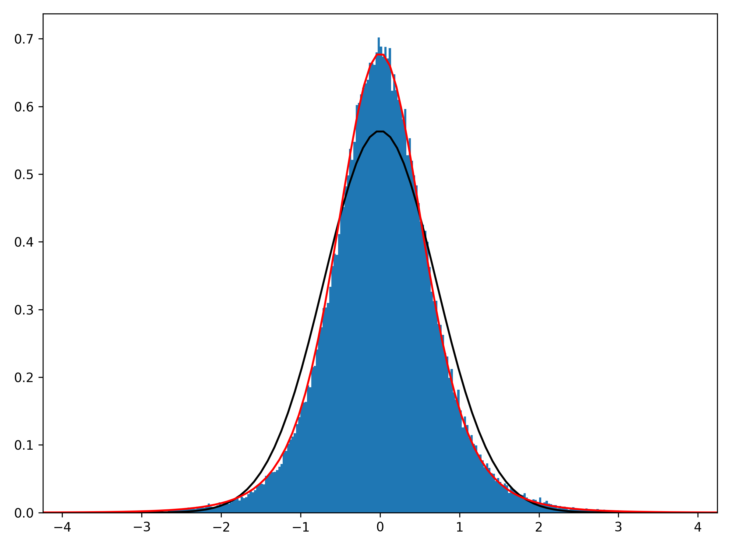
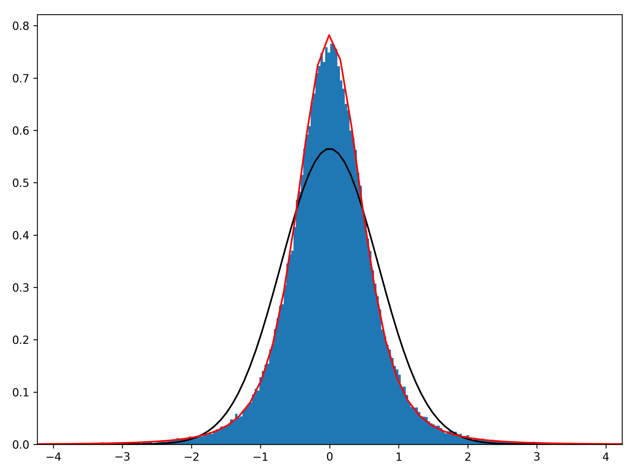
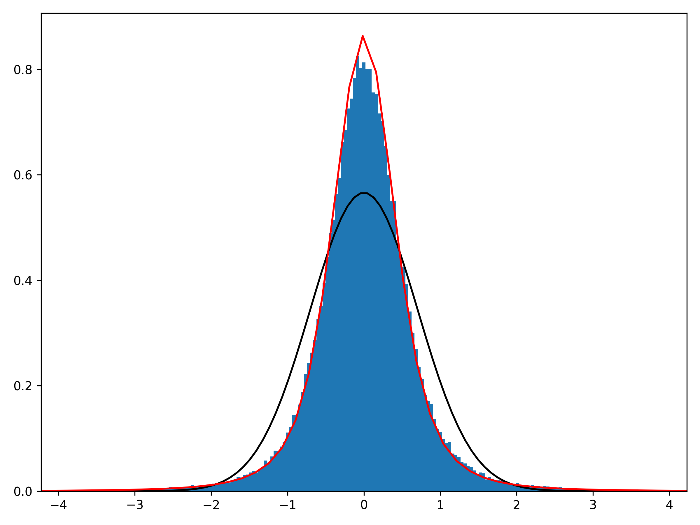
Figure 1: Histogram of 120000 realisations of $\Re\sum_{n\leq x}\alpha(n)\theta^{\Omega(n)/2}$, $x=10000$.

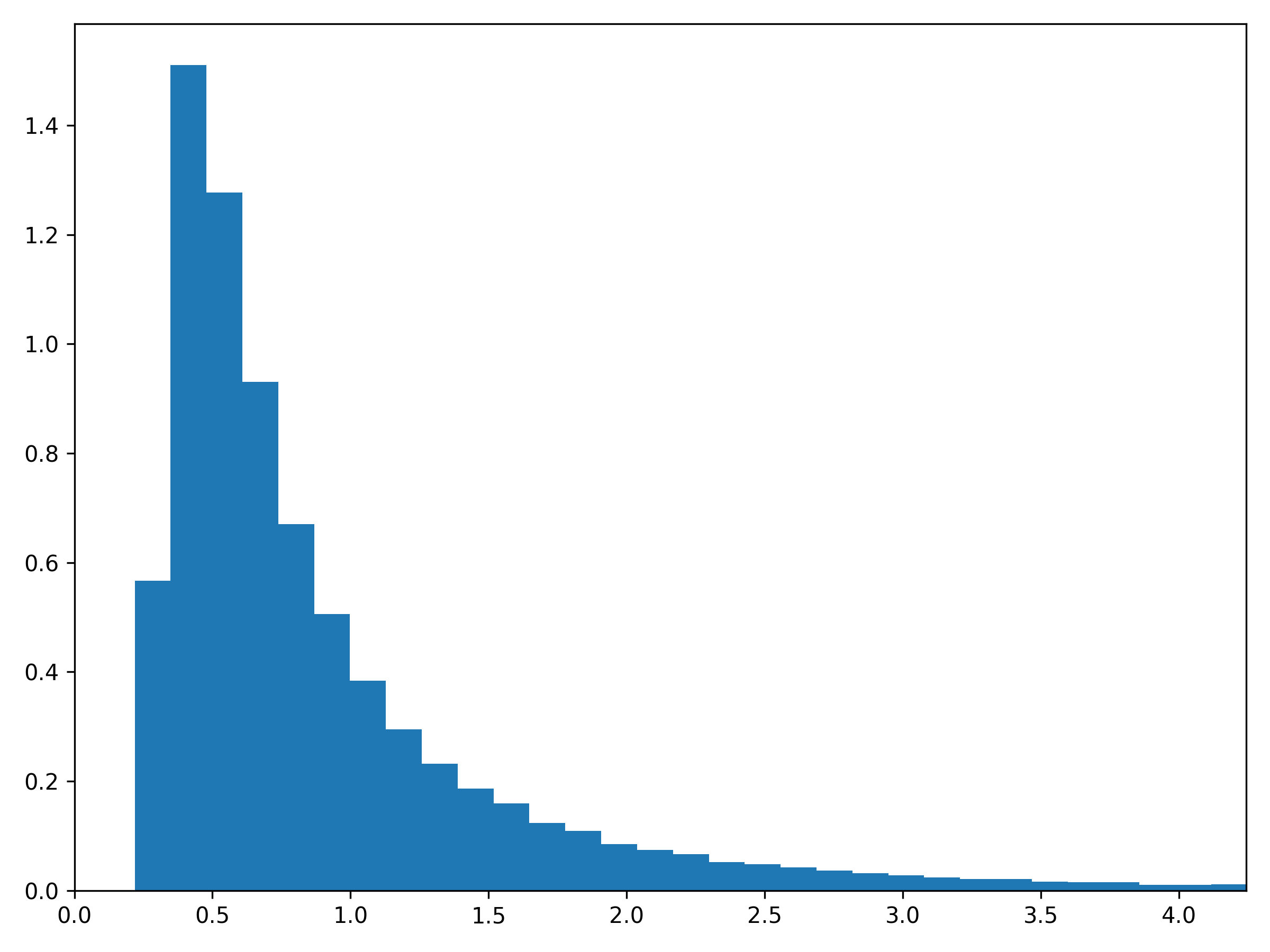
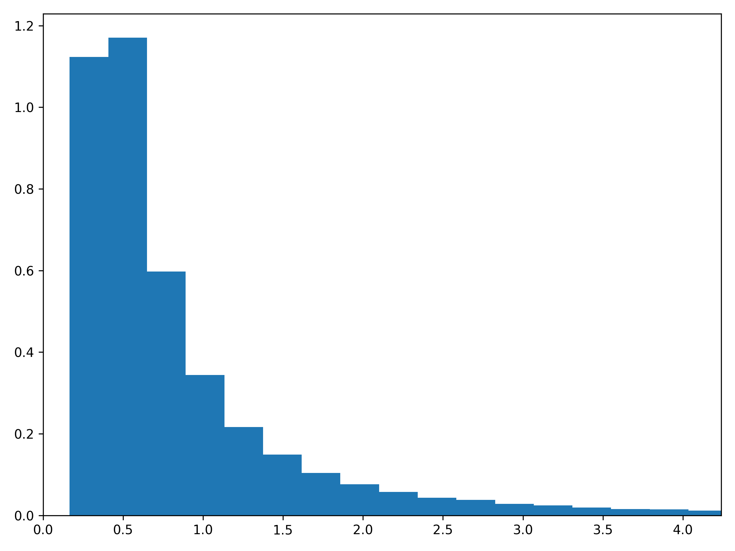
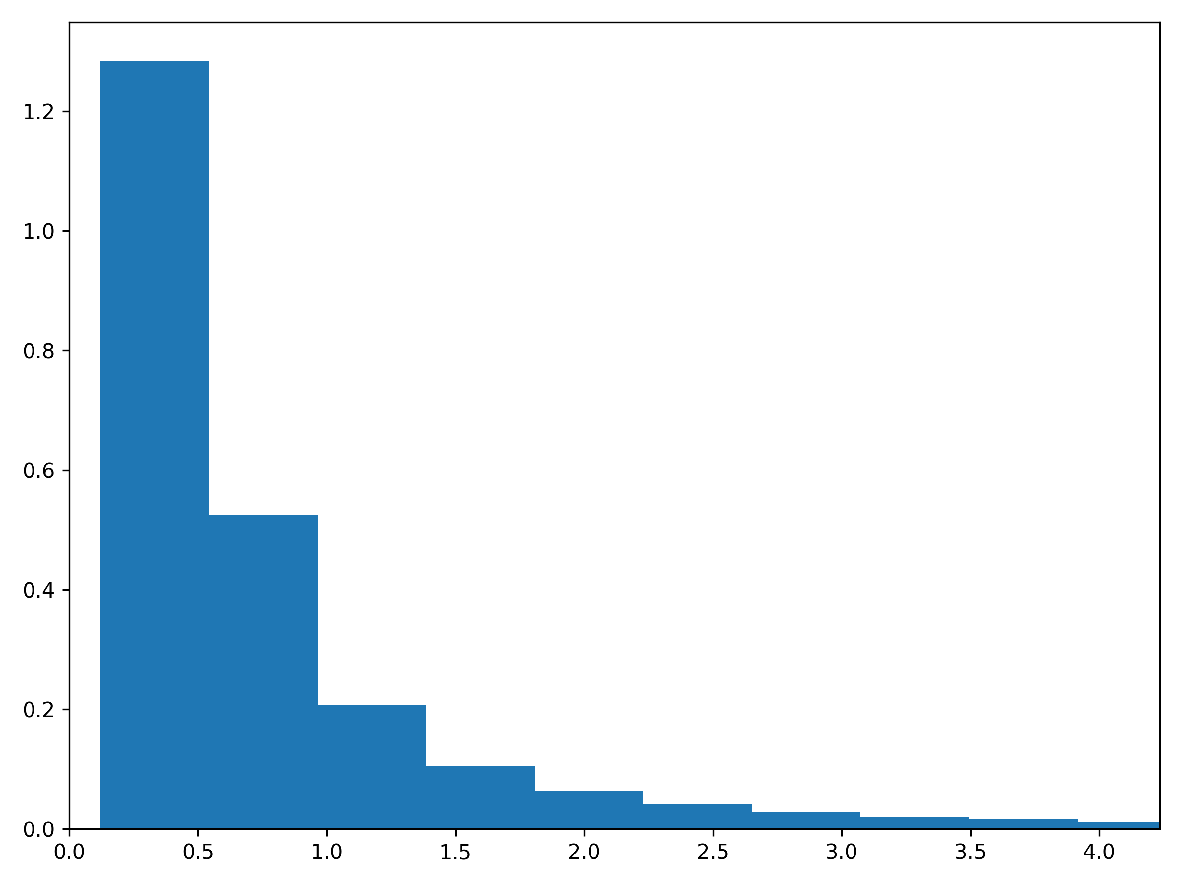
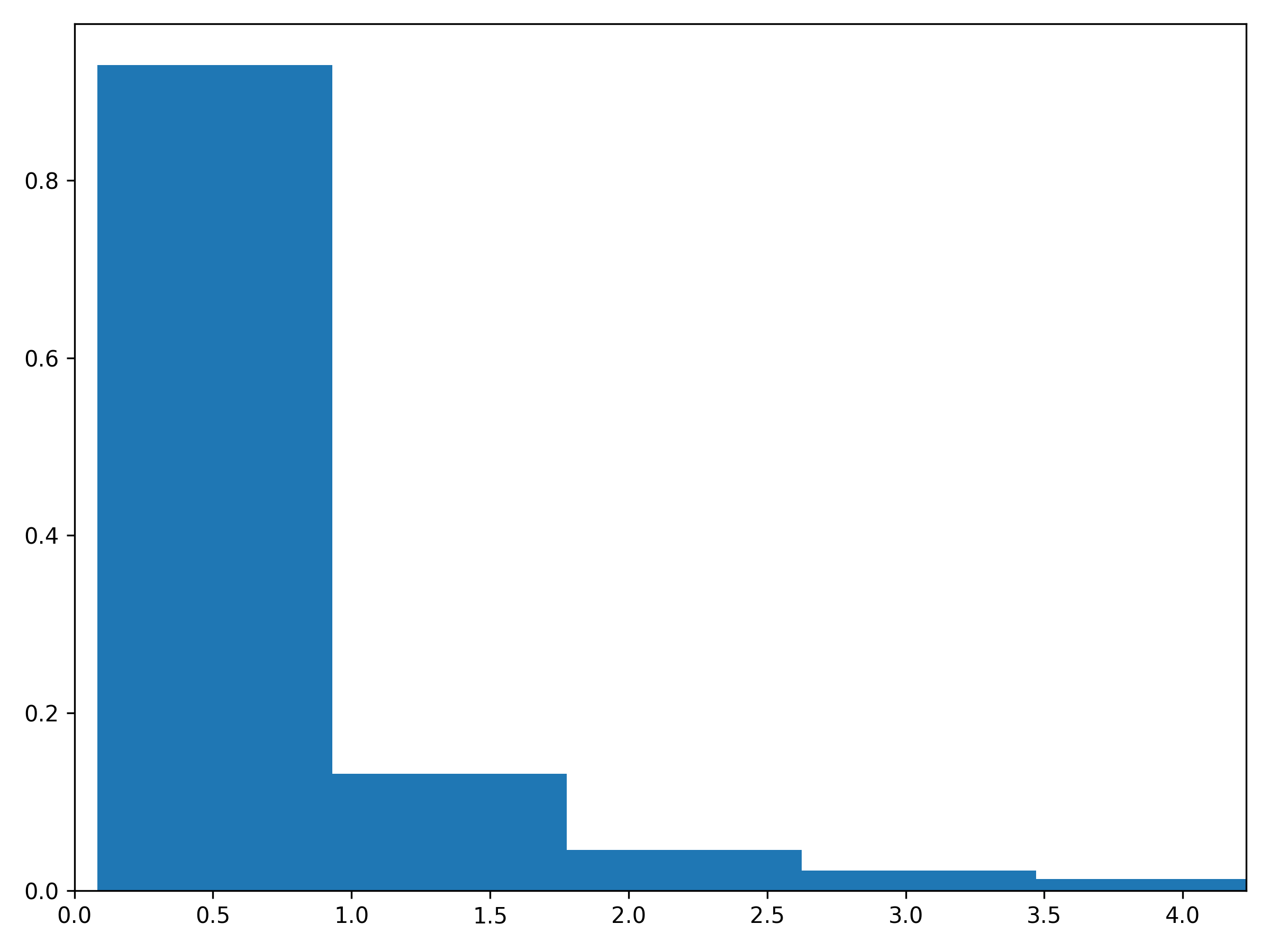
Figure 2: Histogram of 120000 realisations of $\frac{1}{2\pi}\int_{\mathbb{R}}\frac{m_{x,\infty}(ds)}{|\frac{1}{2}+is|^{2}}$, $x=10000$.

2 Structure of the proof of 1.1

2.1 Analogy with the work of Najnudel, Paquette and Simm

Let $\theta>0$. Let $(N_{i})_{i=1}^{\infty}$ be i.i.d. complex random variables distributed according to $N_{i}\sim\mathcal{N}_{\mathbb{C}}(0,1)$. Najnudel, Paquette and Simm [20] investigated the distribution of the random variable $c_{n}$, defined as the coefficient of $u^{n}$ in the power series

$$\exp\bigg{(}\sqrt{\theta}\sum_{i=1}^{\infty}N_{i}\frac{u^{i}}{\sqrt{i}}\bigg{)}.$$ (2.1)

This was motivated by the study of secular coefficients in the circular beta ensemble. It turns out that the asymptotic behaviour of $c_{n}$ as $n\to\infty$ is connected to the Gaussian multiplicative chaos measure on the unit circle, formally defined as

$$\mathrm{GMC}_{\theta}(d\vartheta):=\lim_{r\to 1^{-}}(1-r^{2})^{\theta}\exp\bigg{(}2\sqrt{\theta}\Re\sum_{k=1}^{\infty}N_{k}\frac{(re^{i\vartheta})^{k}}{\sqrt{k}}\bigg{)}d\vartheta,\qquad\vartheta\in[0,2\pi],$$ (2.2)

when $\theta\in(0,1)$ (see [20, Section 1.3] for a discussion of (2.2)). When $\theta\in(0,\tfrac{1}{2})$, they proved that [20, Theorem 1.8]

$$\frac{c_{n}}{\mathbb{E}[|c_{n}|^{2}]^{1/2}}\xrightarrow[n\to\infty]{d}\sqrt{V_{\infty}}\ G$$ (2.3)

where $\displaystyle V_{\infty}$ has law

$$V_{\infty}\overset{d}{=}\frac{1}{2\pi}\int_{0}^{2\pi}\mathrm{GMC}_{\theta}(d\vartheta)$$

and is independent of $G\sim\mathcal{N}_{\mathbb{C}}(0,1)$. Their main tool in proving (2.3) is the martingale central limit theorem, and our proof has a lot in parallel with theirs. To see the analogy between $S_{x}$ and $c_{n}/\mathbb{E}[|c_{n}|^{2}]^{1/2}$, we note that the generating function of $\alpha f$, i.e., its Dirichlet series, is given by

$$\sum_{n=1}^{\infty}\frac{\alpha(n)f(n)}{n^{s}}=\prod_{p}\left(\sum_{i=0}^{\infty}\frac{\alpha(p^{i})f(p^{i})}{p^{is}}\right).$$

Using the central limit theorem and condition (a) in 1.1,

$$\sqrt{\frac{\log n}{n}}\sum_{n\leq p<2n}\alpha(p)f(p)\xrightarrow[n\to\infty]{d}\sqrt{\theta}\ G$$

where $G\sim\mathcal{N}_{\mathbb{C}}(0,1)$. Thus, informally,

$$\sum_{n=1}^{\infty}\frac{\alpha(n)f(n)}{n^{s}}\approx\exp\big{(}\sum_{p}\frac{\alpha(p)f(p)}{p^{s}}\big{)}\approx\exp\bigg{(}\sum_{i=1}^{\infty}2^{-is}\sum_{2^{i}\leq p<2^{i+1}}\alpha(p)f(p)\bigg{)}\approx\exp\bigg{(}\sqrt{\theta}\sum_{i=1}^{\infty}N_{i}2^{-is}\sqrt{\frac{2^{i}}{\log(2^{i})}}\bigg{)}$$

if $\Re s\geq 2$, which resembles the power series in (2.1).

2.2 The (complex) martingale central limit theorem

The following result is deduced in Section B.2 from the real-valued martingale central limit theorem [9, Theorem 3.2 and Corollary 3.1]. It is the main tool behind the proof of 1.1.

Lemma 2.1 (Martingale central limit theorem).

For each $n$, let $(M_{n,j})_{j\leq k_{n}}$ be a complex-valued, mean-zero and square integrable martingale with respect to the filtration $(\mathcal{F}_{j})_{j}$, and $\Delta_{n,j}:=M_{n,j}-M_{n,j-1}$ be the corresponding martingale differences. Suppose the following conditions are satisfied.

• The conditional covariances converge, i.e.,

  $$\sum_{j=1}^{k_{n}}\mathbb{E}\left[\Delta_{n,j}^{2}|\mathcal{F}_{j-1}\right] \xrightarrow[n\to\infty]{p}0$$ (2.4)

  $$\qquad\text{and}\qquad V_{n}:=\sum_{j=1}^{k_{n}}\mathbb{E}\left[|\Delta_{n,j}|^{2}|\mathcal{F}_{j-1}\right] \xrightarrow[n\to\infty]{p}V_{\infty}.$$ (2.5)

• The conditional Lindeberg condition holds: for any $\delta>0$,

  $$\sum_{j=1}^{k_{n}}\mathbb{E}\left[|\Delta_{n,j}|^{2}1_{\{|\Delta_{n,j}|>\delta\}}|\mathcal{F}_{j-1}\right]\xrightarrow[n\to\infty]{p}0.$$

Then

$$M_{n,k_{n}}\xrightarrow[n\to\infty]{d}\sqrt{V_{\infty}}\ G$$

where $G\sim\mathcal{N}_{\mathbb{C}}(0,1)$ is independent of $V_{\infty}$, and the convergence in law is also stable in the sense of Definition B.1.

2.3 A class of functions

Given $\theta>0$ we introduce a subset $\mathcal{M}_{\theta}\subseteq\mathcal{M}$ of all functions $g\in\mathcal{M}$ which satisfy the following mild conditions:

1. For every $n\in\mathbb{N}$, $g(n)\geq 0$.

2. As $t\to\infty$,

   $$\sum_{p\leq t}\frac{g(p)\log p}{p}\sim\theta\log t.$$ (2.6)

3. For $t\geq 2$, $\sum_{p\leq t}g(p)\ll\frac{t}{\log t}$.

4. The following series converges:

   $$\sum_{p}\bigg{(}\frac{g^{2}(p)}{p^{2}}+\sum_{i\geq 2}\frac{g(p^{i})}{p^{i}}\bigg{)}<\infty.$$ (2.7)

5. If $\theta\leq 1$ then we also impose that for $t\geq 2$,

   $$\sum_{p,i\geq 2,\,p^{i}\leq t}g(p^{i})\ll\frac{t}{\log t}.$$

6. As $x\to\infty$,

   $$\sum_{n\leq x}h(n)\sim\frac{e^{-\gamma\theta}}{\Gamma(\theta)}\frac{x}{\log x}\prod_{p\leq x}\left(\sum_{i=0}^{\infty}\frac{h(p^{i})}{p^{i}}\right)$$ (2.8)

   holds for every $h$ of the form $h(\cdot)=g(\cdot)\mathbf{1}_{(\cdot,d)=1}$ for some $d\in\mathbb{N}$.

If $f\in\mathcal{M}$ satisfies the conditions in 1.1 then necessarily $|f|^{2}\in\mathcal{M}_{\theta}$ as a direct consequence of Wirsing’s theorem [25] (see Appendix A for details).

Let $P(1)=1$, and for $n>1$ denote by $P(n)$ the largest prime factor of $n$. Of particular importance to us is the fact that if $g\in\mathcal{M}_{\theta}$ then one can compute the asymptotics of

$$\sum_{n\leq x,\,P(n)\leq x^{\varepsilon}}h(n)$$

for any given $\varepsilon>0$ and any $h$ of the form $h(\cdot)=g(\cdot)\mathbf{1}_{(\cdot,d)=1}$ as an immediate consequence of a classical result of de Bruijn and van Lint [5] (see A.3).

2.4 Overview of the proof

The proof of 1.1 will consist of 4 steps, inspired by [20]. Each step will require (in addition to $f\in\mathcal{M}$) slightly different restrictions on $f$. The conditions in 1.1 will be easily seen to imply all these restrictions. After describing the steps, we will show how, together with 2.1, they imply 1.1. We shall use the following $\sigma$-algebras:

$$\mathcal{F}_{y}:=\sigma(\alpha(p),p\leq y),\qquad\mathcal{F}_{y^{-}}:=\sigma(\alpha(p),p<y),$$ (2.9)

generated by the random variables $\{\alpha(p),p\leq y\}$ and $\{\alpha(p),p<y\}$, respectively.

Step 1: truncation.

Instead of attacking the problem directly, we introduce a truncation parameter $\varepsilon>0$ and define

$$S_{x,\varepsilon}:=\frac{1}{\sqrt{\sum_{n\leq x}|f(n)|^{2}}}\sum_{\begin{subarray}{c}n\leq x\\ P(n)\geq x^{\varepsilon}\\ P(n)^{2}\nmid n\end{subarray}}\alpha(n)f(n).$$

We write

$$S_{x,\varepsilon}=\sum_{x^{\varepsilon}\leq p\leq x}Z_{x,p},\qquad Z_{x,p}:=\frac{1}{\sqrt{\sum_{n\leq x}|f(n)|^{2}}}\sum_{\begin{subarray}{c}\begin{subarray}{c}n\leq x\\ P(n)=p\\ p^{2}\nmid n\end{subarray}\end{subarray}}\alpha(n)f(n).$$ (2.10)

We achieve some technical simplification in using these truncated sums from the beginning, and the following lemma shows we lose little by doing so.

Lemma 2.2.

Let $\theta>0$. Let $f\in\mathcal{M}$ be a function such that $|f|^{2}\in\mathcal{M}_{\theta}$ and

$$\sum_{p,i\geq 2,\,p^{i}\leq x}|f(p^{i})|^{2}=o\left(\frac{x}{(\log x)^{2}}\right)$$ (2.11)

as $x\to\infty$. Then $\limsup_{\varepsilon\to 0^{+}}\limsup_{x\to\infty}\mathbb{E}\left[|S_{x}-S_{x,\varepsilon}|^{2}\right]=0$.

Ultimately, we apply 2.1 to $S_{x,\varepsilon}$.

Step 2: Lindeberg condition.

The proof of the following lemma will be given in Section 3.2.

Lemma 2.3.

Let $\theta>0$. Let $f\in\mathcal{M}$ be a function such that $|f|^{2}\in\mathcal{M}_{\theta}$ and

$$\sum_{p}\bigg{(}\sum_{i\geq 2}\frac{|f(p^{i})|^{2}i}{p^{i}}\bigg{)}^{2}<\infty,$$ (2.12)

$$\sum_{p\leq x}\left(|f(p^{2})|^{2}+|f(p)|^{4}\right)\ll x^{2}(\log x)^{-2\theta-4}.$$ (2.13)

Then $\limsup_{x\to\infty}\sum_{x^{\varepsilon}\leq p\leq x}\mathbb{E}[|Z_{x,p}|^{4}]=0$ for every $\varepsilon>0$.

We claim 2.3 implies that for any $\delta>0$,

$$\sum_{x^{\varepsilon}\leq p\leq x}\mathbb{E}\left[|Z_{x,p}|^{2}1_{\{|Z_{x,p}|>\delta\}}|\mathcal{F}_{p^{-}}\right]\xrightarrow[x\to\infty]{p}0.$$ (2.14)

Indeed, the left-hand side of the above can be upper bounded by

$$\delta^{-2}\sum_{x^{\varepsilon}\leq p\leq x}\mathbb{E}\left[|Z_{x,p}|^{4}|\mathcal{F}_{p^{-}}\right]$$

using Cauchy–Schwarz, and

$$\mathbb{E}\bigg{[}\sum_{x^{\varepsilon}\leq p\leq x}\mathbb{E}\left[|Z_{x,p}|^{4}|\mathcal{F}_{p^{-}}\right]\bigg{]}=\sum_{x^{\varepsilon}\leq p\leq x}\mathbb{E}\left[|Z_{x,p}|^{4}\right]$$

vanishes when we first send $x\to\infty$ and then $\varepsilon\to 0^{+}$ by 2.3. This shows that the convergence (2.14) holds in $L^{1}$, and in particular in probability. Observe (2.14) corresponds to the Lindeberg condition in 2.1.

Step 3: approximating the conditional variance.

Let

$$T_{x,\varepsilon}:=\sum_{x^{\varepsilon}\leq p\leq x}\mathbb{E}\left[|Z_{x,p}|^{2}\mid\mathcal{F}_{p^{-}}\right]$$

and

$$U_{x}:=\bigg{(}\sum_{n\leq x}|f(n)|^{2}\left(\frac{1}{n}-\frac{1}{x}\right)\bigg{)}^{-1}\int_{1}^{x}\frac{|s_{t}|^{2}}{t}dt,\qquad s_{t}:=\frac{1}{\sqrt{t}}\sum_{n\leq t}\alpha(n)f(n).$$ (2.15)

Given $\theta>0$, define $\rho_{\theta}\colon(0,\infty)\to(0,\infty)$ via $\rho_{\theta}(t)=t^{\theta-1}/\Gamma(\theta)$ for $t\leq 1$ and by

$$t\rho_{\theta}(t)=\theta\int_{t-1}^{t}\rho_{\theta}(v)dv$$

for $t>1$. See Smida [23] for an asymptotic investigation of $\rho_{\theta}$, which tends rapidly to $0$. Let

$$C_{\varepsilon}:=\theta\int_{\varepsilon}^{1}\frac{(1-v)^{\theta-1}}{v}\frac{\Gamma(\theta)\rho_{\theta}\left(\frac{1-v}{v}\right)}{((1-v)/v)^{\theta-1}}dv.$$ (2.16)

It was shown in [20, Equation (4.38)] that $\lim_{\varepsilon\to 0^{+}}C_{\varepsilon}=1$.

Proposition 2.4.

Let $\theta\in(0,\frac{1}{2})$. Let $f\in\mathcal{M}$ be a function such that $|f|^{2}\in\mathcal{M}_{\theta}$. Suppose there exists $c>0$ such that $|f(p)|=O(p^{\frac{1}{2}-c})$ and $|f(p^{k})|^{2}=O(2^{k(1-c)})$ for all $k\geq 2$ and primes $p$. Then $\lim_{x\to\infty}\mathbb{E}[|T_{x,\varepsilon}-C_{\varepsilon}U_{x}|^{2}]=0$.

When establishing Proposition 2.4 we shall assume $x$ is sufficiently large as this implies that the denominator $\sum_{n\leq x}|f(n)|^{2}(1/n-1/x)\geq 0$ in $U_{x}$ is not $0$. The denominator was chosen as it forces

$$\mathbb{E}[U_{x}]\equiv 1.$$

Indeed, $\mathbb{E}[|s_{t}|^{2}]=\sum_{n\leq t}|f(n)|^{2}/t$ by (1.1) and so

$$\mathbb{E}\left[\int_{1}^{x}\frac{|s_{t}|^{2}}{t}dt\right]=\sum_{n\leq x}|f(n)|^{2}\int_{n}^{x}\frac{dt}{t^{2}}=\sum_{n\leq x}|f(n)|^{2}\left(\frac{1}{n}-\frac{1}{x}\right).$$

Step 4: convergence of conditional variance.

To conclude the proof of 1.1, we need to identify the limit of $U_{x}$ which is the subject of Section 4. As we shall see in Section 4, the task of identifying the limit of $U_{x}$ is closely related to understanding the random Euler product

$$A_{y}(s):=\prod_{p\leq y}\bigg{(}1+\sum_{k\geq 1}\frac{\alpha(p)^{k}f(p^{k})}{p^{ks}}\bigg{)}=\sum_{P(n)\leq y}\frac{\alpha(n)f(n)}{n^{s}},$$

and will require the following probabilistic ingredient.

Theorem 2.5.

Let $\theta\in(0,\frac{1}{2})$, and $f\in\mathcal{M}$ be a function such that $|f|^{2}\in\mathbf{P}_{\theta}$ and

$$\sum_{p}\bigg{(}\frac{|f(p)|^{3}}{p^{3/2}}+\frac{|f(p^{2})|^{2}}{p^{2}}+\sum_{k\geq 3}\frac{|f(p^{k})|^{2}}{p^{k/2}}\bigg{)}<\infty.$$ (2.17)

Write

$$\sigma_{t}=\tfrac{1}{2}\left(1+\frac{1}{\log t}\right)\qquad\text{and}\qquad m_{y,t}(ds):=\frac{|A_{y}(\sigma_{t}+is)|^{2}}{\mathbb{E}\left[|A_{y}(\sigma_{t}+is)|^{2}\right]}ds,\qquad s\in\mathbb{R}.$$ (2.18)

Then there exists a nontrivial random Radon measure $m_{\infty}(ds)$ on $\mathbb{R}$ such that the following are true: for any bounded interval $I$ and any test function $h\in C(I)$, we have

$$(i)\quad m_{y,\infty}(h)\xrightarrow[y\to\infty]{L^{2}}m_{\infty}(h)\qquad\text{and}\qquad(ii)\quad m_{\infty,t}(h)\xrightarrow[t\to\infty]{L^{2}}m_{\infty}(h)$$ (2.19)

and in particular the above convergence also holds in probability. Moreover, the limiting measure $m_{\infty}(ds)$ is supported on $\mathbb{R}$ almost surely.

We will obtain from 2.5 the following result.

Lemma 2.6.

Under the same setting as 2.5, we have

$$U_{x}\xrightarrow[x\to\infty]{p}\frac{1}{2\pi}\int_{\mathbb{R}}\frac{m_{\infty}(ds)}{|\frac{1}{2}+is|^{2}}$$ (2.20)

and the limit is almost surely finite and strictly positive.

For the moment let us assume the validity of all the results presented in the current section. We are ready to explain:

Proof of 1.1.

Let $\varepsilon>0$ be fixed. Since $Z_{x,p}$ is linear in $\alpha(p)$ by construction, for any $x>0$ we automatically obtain $\sum_{x^{\varepsilon}\leq p\leq x}\mathbb{E}[Z_{x,p}^{2}|\mathcal{F}_{p^{-}}]=0$ almost surely. Moreover, we have

$$T_{x,\varepsilon}:=\sum_{x^{\varepsilon}\leq p\leq x}\mathbb{E}\left[|Z_{x,p}|^{2}\mid\mathcal{F}_{p^{-}}\right]\xrightarrow[x\to\infty]{p}\frac{C_{\varepsilon}}{2\pi}\int_{\mathbb{R}}\frac{m_{\infty}(ds)}{|\tfrac{1}{2}+is|^{2}}=C_{\varepsilon}V_{\infty}$$

by Proposition 2.4 and 2.6. Combining this with 2.3 (which implies the conditional Lindeberg condition), we see that the martingale sequence associated to $S_{x,\varepsilon}$ satisfies all assumptions in 2.1, and thus $S_{x,\varepsilon}\xrightarrow[x\to\infty]{d}\sqrt{C_{\varepsilon}V_{\infty}}G$ where the distributional convergence is also stable.

To establish the stable convergence of $S_{x}$, it is helpful to use the formulation (B.2) in the language of weak convergence: we would like to show that

$$\lim_{x\to\infty}\mathbb{E}\left[Y\widetilde{h}(S_{x})\right]=\mathbb{E}\left[Y\widetilde{h}(\sqrt{V_{\infty}}G)\right]$$

for any bounded $\mathcal{F}_{\infty}$-measurable random variable $Y$ and any bounded continuous function $\widetilde{h}\colon\mathbb{C}\to\mathbb{R}$. By a density argument, it suffices to establish this claim for bounded Lipschitz functions $\widetilde{h}$. Consider

$$\left|\mathbb{E}\left[Y\widetilde{h}(S_{x})\right]-\mathbb{E}\left[Y\widetilde{h}(\sqrt{V_{\infty}}G)\right]\right| \leq\left|\mathbb{E}\left[Y\widetilde{h}(S_{x,\varepsilon})\right]-\mathbb{E}\left[Y\widetilde{h}(\sqrt{C_{\varepsilon}V_{\infty}}G)\right]\right|$$

$$\qquad+\mathbb{E}\left[Y\left|\widetilde{h}(S_{x})-\widetilde{h}(S_{x,\varepsilon})\right|\right]+\mathbb{E}\left[Y\left|\widetilde{h}(\sqrt{V_{\infty}}G)-\widetilde{h}(\sqrt{C_{\varepsilon}V_{\infty}}G)\right|\right].$$

We see that the first term on the right-hand side converges to $0$ as $x\to\infty$ as a consequence of the stable convergence of $S_{x,\varepsilon}$, whereas the third term converges to $0$ as $\varepsilon\to 0^{+}$ as a consequence of dominated convergence. Meanwhile, the middle term is bounded by

$$\|\widetilde{h}\|_{\mathrm{Lip}}\mathbb{E}[Y^{2}]^{1/2}\mathbb{E}\left[\left|S_{x}-S_{x,\varepsilon}\right|^{2}\right]^{\frac{1}{2}}$$

which also vanishes in the limit as $x\to\infty$ and then $\varepsilon\to 0^{+}$ by 2.2. This completes the proof of 1.1. ∎

Outline.

The remainder of the article is organised as follows.

• In Section 3, we shall carry out the first three steps, proving 2.2, 2.3 and Proposition 2.4.

• In Section 4, we shall carry out the fourth step, establishing 2.5 and 2.6. Towards the end we shall also provide the proof of 1.2, and discuss extension to larger values of $q$.

• In Section 5, we treat the Rademacher case, and highlight the changes needed for the proof of 1.3 and 1.4.

• Finally, we collect various results about mean values of nonnegative multiplicative functions and abstract probability ingredients in the two appendices.

3 Proofs of 2.2, 2.3 and Proposition 2.4

3.1 Truncation: proof of 2.2

By (1.1),

$$\mathbb{E}\left[|S_{x}-S_{x,\varepsilon}|^{2}\right]=(\sum_{n\leq x}|f(n)|^{2})^{-1}\sum_{\begin{subarray}{c}n\leq x\\ P(n)<x^{\varepsilon}\text{ or }P(n)^{2}\mid n\end{subarray}}|f(n)|^{2}=A_{1,\varepsilon}+A_{2,\varepsilon}$$

where

$$A_{1,\varepsilon}:=(\sum_{n\leq x}|f(n)|^{2})^{-1}\sum_{\begin{subarray}{c}n\leq x\\ P(n)<x^{\varepsilon}\end{subarray}}|f(n)|^{2},\qquad A_{2,\varepsilon}:=(\sum_{n\leq x}|f(n)|^{2})^{-1}\sum_{\begin{subarray}{c}n\leq x\\ P(n)\geq x^{\varepsilon}\\ P(n)^{2}\mid n\end{subarray}}|f(n)|^{2}.$$ (3.1)

By A.3 with $g=|f|^{2}$,

$$\limsup_{x\to\infty}A_{1,\varepsilon}=\Gamma(\theta)\rho_{\theta}(1/\varepsilon)\varepsilon^{\theta-1}$$

which tends to $0$ as $\varepsilon\to 0^{+}$ [23]. In particular, $\limsup_{\varepsilon\to 0^{+}}\limsup_{x\to\infty}A_{1,\varepsilon}=0$. To estimate $A_{2,\varepsilon}$ we denote $P(n)$ by $p$, and the multiplicity of $P(n)$ in $n$ by $i$ (i.e., $P(n)^{i}\mid n$ but $P(n)^{i+1}\nmid i$), so

$$\begin{split}A_{2,\varepsilon}&=(\sum_{n\leq x}|f(n)|^{2})^{-1}\sum_{p\geq x^{\varepsilon}}\sum_{i\geq 2}|f(p^{i})|^{2}\sum_{\begin{subarray}{c}m\leq x/p^{i}\\ P(m)<p\end{subarray}}|f(m)|^{2}\\ &\leq(\sum_{n\leq x}|f(n)|^{2})^{-1}\sum_{p\geq x^{\varepsilon}}\sum_{i\geq 2}|f(p^{i})|^{2}\sum_{m\leq x/p^{i}}|f(m)|^{2}\end{split}$$ (3.2)

where $m$ stands for $n/p^{i}$. Considering $p^{i}\leq\sqrt{x}$ and $p^{i}>\sqrt{x}$ separately in (3.2), we deduce using (2.8) applied twice (with $f=|g|^{2}$) that

$$A_{2,\varepsilon}\ll\sum_{\begin{subarray}{c}p\geq x^{\varepsilon},\,i\geq 2\\ p^{i}\leq\sqrt{x}\end{subarray}}\frac{|f(p^{i})|^{2}}{p^{i}}+\log x\sum_{\begin{subarray}{c}p\geq x^{\varepsilon},\,i\geq 2\\ x\geq p^{i}>\sqrt{x}\end{subarray}}\frac{|f(p^{i})|^{2}}{p^{i}}.$$

We bound the last sums using (2.11), finding that for any fixed $\varepsilon>0$, $\limsup_{x\to\infty}A_{2,\varepsilon}=0$.

3.2 Lindeberg condition: proof of 2.3

By (1.1),

$$\sum_{x^{\varepsilon}\leq p\leq x}\mathbb{E}\left[|Z_{x,p}|^{4}\right]=(\sum_{n\leq x}|f(n)|^{2})^{-2}\sum_{x^{\varepsilon}\leq p\leq x}\sum_{\begin{subarray}{c}ab=cd\\ a,b,c,d\leq x\\ P(a)=P(b)=P(c)=P(d)=p\\ P(a)^{2}\nmid a,b,c,d\end{subarray}}f(a)f(b)\overline{f(c)f(d)}.$$ (3.3)

The inner sum in the right-hand side of (3.3) can be written as

$$\sum_{\begin{subarray}{c}ab=cd\\ a,b,c,d\leq x\\ P(a)=P(b)=P(c)=P(d)=p\\ P(a)^{2}\nmid a,b,c,d\end{subarray}}f(a)f(b)\overline{f(c)f(d)}=\sum_{\begin{subarray}{c}m\leq x^{2}\\ P(m)=p\end{subarray}}h(m),\qquad h(m):=\bigg{|}\sum_{\begin{subarray}{c}ab=m\\ P(a)=P(b)\\ a,b\leq x\\ P(m)^{2}\nmid a,b\end{subarray}}f(a)f(b)\bigg{|}^{2}.$$

We write $p^{2}\mid\mid m$ to indicate that $p^{2}$ divides $m$ but $p^{3}$ does not. We have the pointwise bound $h(m)\leq(|f|*|f|)^{2}(m)\cdot\mathbf{1}_{P(m)^{2}\mid\mid m}$ so that

$$\sum_{\begin{subarray}{c}ab=cd\\ a,b,c,d\leq x\\ P(a)=P(b)=P(c)=P(d)=p\\ P(a)^{2}\nmid a,b,c,d\end{subarray}}f(a)f(b)\overline{f(c)f(d)}\leq\sum_{\begin{subarray}{c}m\leq x^{2}\\ P(m)=p\\ P(m)^{2}\mid\mid m\end{subarray}}H(m),\qquad H:=(|f|*|f|)^{2}.$$

It follows that

$$\sum_{x^{\varepsilon}\leq p\leq x}\sum_{\begin{subarray}{c}ab=cd\\ a,b,c,d\leq x\\ P(a)=P(b)=P(c)=P(d)=p\\ P(a)^{2}\nmid a,b,c,d\end{subarray}}f(a)f(b)\overline{f(c)f(d)}\leq\sum_{x^{\varepsilon}\leq p\leq x}\sum_{\begin{subarray}{c}p^{2}\mid\mid m\leq x^{2}\\ P(m)\leq p\end{subarray}}H(m)=\sum_{x^{\varepsilon}\leq p\leq x}H(p^{2})\sum_{\begin{subarray}{c}m^{\prime}\leq x^{2}/p^{2}\\ P(m^{\prime})<p\end{subarray}}H(m^{\prime})$$ (3.4)

where $m^{\prime}$ stands for $m/p^{2}$. Next,

$$\sum_{\begin{subarray}{c}m^{\prime}\leq x^{2}/p^{2}\\ P(m^{\prime})<p\end{subarray}}H(m^{\prime})\leq\sum_{m^{\prime}\leq x^{2}/p^{2}}H(m^{\prime})\leq\frac{x^{2}}{p^{2}}\sum_{m^{\prime}\leq x^{2}/p^{2}}\frac{H(m^{\prime})}{m^{\prime}}\leq\frac{x^{2}}{p^{2}}\prod_{q\leq x^{2}/p^{2}}\left(\sum_{i=0}^{\infty}\frac{H(q^{i})}{q^{i}}\right).$$ (3.5)

Our assumptions on $|f(p)|$ and $|f(p^{i})|$ in (2.7) (with $g=|f|^{2}$) and (2.12) imply $\sum_{q,i\geq 2}H(q^{i})/q^{i}<\infty$, and so

$$\prod_{q\leq x^{2}/p^{2}}\left(\sum_{i=0}^{\infty}\frac{H(q^{i})}{q^{i}}\right)\ll\prod_{q\leq x^{2}/p^{2}}\left(1+\frac{H(q)}{q}\right).$$ (3.6)

Since $H(q)=4|f(q)|^{2}$, we have

$$\prod_{q\leq x^{2}/p^{2}}\bigg{(}1+\frac{H(q)}{q}\bigg{)}\leq\prod_{q\leq x^{2}}\bigg{(}1+\frac{H(q)}{q}\bigg{)}=(\log x)^{4\theta+o(1)}$$

by (2.6) and (2.7) (with $g=|f|^{2}$). Thus, (3.5) and (3.6) imply

$$\sum_{x^{\varepsilon}\leq p\leq x}H(p^{2})\sum_{\begin{subarray}{c}m^{\prime}\leq x^{2}/p^{2}\\ P(m^{\prime})<p\end{subarray}}H(m^{\prime})\ll x^{2}(\log x)^{4\theta+o(1)}\sum_{x^{\varepsilon}\leq p\leq x}\frac{H(p^{2})}{p^{2}}.$$ (3.7)

By definition of $H$, $H(p^{2})\ll|f(p^{2})|^{2}+|f(p)|^{4}$. Our assumptions on $f(p)$ and $f(p^{2})$ in (2.13) show that the $p$-sum in the right-hand side of (3.7) is $\ll_{\varepsilon}(\log x)^{-2\theta-3}$. We conclude by plugging (3.7) in (3.4) and then (3.4) in (3.3), and noting $\sum_{n\leq x}|f(n)|^{2}=x(\log x)^{\theta-1+o(1)}$ by (2.8) with $h=|f|^{2}$ and A.1.

3.3 Approximating conditional variance: proof of Proposition 2.4

Given $f\in\mathcal{M}$ we define

$$R:=\sum_{(n_{1},n_{2})=1}\frac{1}{\max\{n_{1},n_{2}\}^{2}}\prod_{i=1}^{2}\bigg{|}\sum_{g_{i}\mid n_{i}^{\infty}}\frac{\overline{f(g_{i})}f(g_{i}n_{i})}{g_{i}}\bigg{|}^{2}\bigg{(}\sum_{h\mid(n_{1}n_{2})^{\infty}}\frac{|f^{2}(h)|}{h}\bigg{)}^{-2},$$

where the outer sum is over all pairs of coprime positive integers $n_{1}$ and $n_{2}$. The notation ‘$g\mid n^{\infty}$’ indicates that $g$ ranges over all positive integers whose prime factors divide $n$, e.g., if $n=p$ then $g$ ranges over all powers of $p$. If $f$ is completely multiplicative then

$$R=\sum_{(n_{1},n_{2})=1}\frac{|f(n_{1})|^{2}|f(n_{2})|^{2}}{\max\{n_{1},n_{2}\}^{2}}.$$

The proof of Proposition 2.4 is broken into three parts:

Lemma 3.1.

Let $\theta\in(0,\frac{1}{2})$. Suppose $f\in\mathcal{M}$ satisfies $|f|^{2}\in\mathcal{M}_{\theta}$, and that

$$R^{\prime}:=\sum_{(n_{1},n_{2})=1}\frac{1}{\max\{n_{1},n_{2}\}^{2}}\prod_{i=1}^{2}\bigg{(}\sum_{g_{i}\mid n_{i}^{\infty}}\frac{|\overline{f(g_{i})}f(g_{i}n_{i})|}{g_{i}}\bigg{)}^{2}\bigg{(}\sum_{h\mid(n_{1}n_{2})^{\infty}}\frac{|f^{2}(h)|}{h}\bigg{)}^{-2}$$ (3.8)

converges. Then, as $x\to\infty$,

$$\mathbb{E}[U_{x}^{2}] \to R,$$ (3.9)

$$\mathbb{E}[T_{x,\varepsilon}U_{x}] \to C_{\varepsilon}R,$$ (3.10)

$$\mathbb{E}[T_{x,\varepsilon}^{2}] \to C^{2}_{\varepsilon}R.$$ (3.11)

Note that $R^{\prime}$ dominates $R$. Before embarking on the proof of 3.1, we explain why (3.8) converges when the assumptions of Proposition 2.4 hold. In fact, we estimate the tail of (3.8). Let

$$\widetilde{f}(n):=\sum_{g\mid n^{\infty}}\frac{|\overline{f(g)}f(gn)|}{g}.$$

By the triangle inequality and the fact that $f(1)=1$,

$$\sum_{\begin{subarray}{c}(n_{1},n_{2})=1\\ \max\{n_{1},n_{2}\}\geq T\end{subarray}}\frac{1}{\max\{n_{1},n_{2}\}^{2}}\prod_{i=1}^{2}\big{(}\sum_{g_{i}\mid n_{i}^{\infty}}\frac{|\overline{f(g_{i})}f(g_{i}n_{i})|}{g_{i}}\big{)}^{2}\big{(}\sum_{h\mid(n_{1}n_{2})^{\infty}}\frac{|f^{2}(h)|}{h}\big{)}^{-2}\leq\sum_{\max\{n_{1},n_{2}\}\geq T}\frac{(\widetilde{f}(n_{1})\widetilde{f}(n_{2}))^{2}}{\max\{n_{1},n_{2}\}^{2}}.$$

By Cauchy–Schwarz,

$$\widetilde{f}(p^{i})^{2}\ll|f(p^{i})|^{2}+\sum_{j\geq 1}\frac{|f(p^{j})|^{2}}{p^{j}}\sum_{j\geq 1}\frac{|f(p^{i+j})|^{2}}{p^{j}},\quad(\widetilde{f}(p)-|f(p)|)^{2}\leq\sum_{j\geq 1}\frac{|f(p^{j})|^{2}}{p^{j}}\sum_{j\geq 1}\frac{|f(p^{j+1})|^{2}}{p^{j}}.$$ (3.12)

From (3.12) we see that our assumptions on $f$ imply

$$\begin{split}&\sum_{p\leq T}\widetilde{f}(p)^{2}\log p\ll T\qquad(T\geq 2),\qquad\sum_{p\leq T}\frac{\widetilde{f}(p)^{2}\log p}{p}\sim\theta\log T\qquad(T\to\infty),\\ &\sum_{p,i\geq 2}\frac{\widetilde{f}(p^{i})^{2}\log(p^{i})}{p^{i}}<\infty.\end{split}$$ (3.13)

By A.5 and (3.13) we have

$$\sum_{n\leq T}\widetilde{f}(n)^{2}\ll\frac{T}{\log T}\sum_{n\leq T}\frac{\widetilde{f}(n)^{2}}{n}\leq\frac{T}{\log T}\prod_{p\leq T}\sum_{i=0}^{\infty}\bigg{(}\frac{\widetilde{f}(p^{i})^{2}}{p^{i}}\bigg{)}\ll\frac{T}{\log T}\prod_{p\leq T}\bigg{(}1+\frac{\widetilde{f}(p)^{2}}{p}\bigg{)}\ll T(\log T)^{\theta-1+o(1)}$$ (3.14)

uniformly for $T\geq 2$, and so

$$\sum_{\max\{n_{1},n_{2}\}\geq T}\frac{(\widetilde{f}(n_{1})\widetilde{f}(n_{2}))^{2}}{\max\{n_{1},n_{2}\}^{2}}\ll\sum_{n\geq T}\frac{\widetilde{f}(n)^{2}(\log(n+1))^{\theta-1+o(1)}}{n}\ll(\log T)^{2\theta-1+o(1)}$$

where we used (3.14) and the fact that $\theta<\tfrac{1}{2}$. Here $n$ stands for $\max\{n_{1},n_{2}\}$.

3.3.1 Proof of first part of 3.1

We introduce

$$F_{m}(x):=\sum_{\begin{subarray}{c}h\leq x\\ (h,m)=1\end{subarray}}|f(h)|^{2}\left(\frac{1}{h}-\frac{1}{x}\right),\qquad S_{1}(x,m,d):=\frac{F_{m}(x/d)}{F_{1}(x)}.$$ (3.15)

The proof of (3.9) relies on the following identity which holds for all multiplicative functions.

Lemma 3.2.

Let $f\in\mathcal{M}$. We have

$$\mathbb{E}[U_{x}^{2}]=\sum_{\begin{subarray}{c}n_{i}\leq x\\ (n_{1},n_{2})=1\end{subarray}}\frac{1}{\max\{n_{1},n_{2}\}^{2}}\left|\sum_{g_{i}\mid n_{i}^{\infty}}\frac{\overline{f(g_{1})}f(g_{1}n_{1})f(g_{2})\overline{f(g_{2}n_{2})}}{g_{1}g_{2}}S_{1}(x,n_{1}n_{2},\max\{n_{1},n_{2}\}g_{1}g_{2})\right|^{2}.$$ (3.16)

Proof.

By definition,

$$\mathbb{E}[U_{x}^{2}]=F_{1}(x)^{-2}S,\qquad S:=\int_{1}^{x}\int_{1}^{x}\frac{\mathbb{E}\left[|s_{t}|^{2}|s_{r}|^{2}\right]}{tr}dtdr.$$

By (1.1),

$$\mathbb{E}\left[|s_{t}|^{2}|s_{r}|^{2}\right]=\frac{1}{tr}\sum_{\begin{subarray}{c}n_{1},n_{2}\leq t\\ m_{1},m_{2}\leq r\\ n_{1}m_{1}=n_{2}m_{2}\end{subarray}}f(n_{1})\overline{f(n_{2})}f(m_{1})\overline{f(m_{2})}.$$

It follows that

$$S =\sum_{\begin{subarray}{c}n_{1},n_{2},m_{1},m_{2}\leq x\\ n_{1}m_{1}=n_{2}m_{2}\end{subarray}}f(n_{1})f(m_{1})\overline{f(n_{2})f(m_{2})}\int_{\max\{n_{1},n_{2}\}}^{x}\int_{\max\{m_{1},m_{2}\}}^{x}\frac{dtdr}{t^{2}r^{2}}$$

$$=\sum_{\begin{subarray}{c}n_{1},n_{2},m_{1},m_{2}\leq x\\ n_{1}m_{1}=n_{2}m_{2}\end{subarray}}f(n_{1})f(m_{1})\overline{f(n_{2})f(m_{2})}\left(\frac{1}{\max\{n_{1},n_{2}\}}-\frac{1}{x}\right)\left(\frac{1}{\max\{m_{1},m_{2}\}}-\frac{1}{x}\right).$$

We parametrize the solutions to $n_{1}m_{1}=n_{2}m_{2}$. We let $g_{1}:=(n_{1},n_{2})$ and $n^{\prime}_{i}:=n_{i}/g_{1}$ ($i=1,2$). Since $(n^{\prime}_{1},n^{\prime}_{2})=1$ and $n^{\prime}_{1}m_{1}=n^{\prime}_{2}m_{2}$ we must have $m_{1}=g_{2}n^{\prime}_{2}$ and $m_{2}=g_{2}n^{\prime}_{1}$ for some $g_{2}$. Conversely, given coprime $n^{\prime}_{1}$ and $n^{\prime}_{2}$, and arbitrary $g_{1},g_{2}$, we can construct a solution to $n_{1}m_{1}=n_{2}m_{2}$ via $n_{i}=g_{1}n^{\prime}_{i}$, $m_{1}=g_{2}n^{\prime}_{2}$ and $m_{2}=g_{2}n^{\prime}_{1}$. So

$$S=\sum_{\begin{subarray}{c}n^{\prime}_{1},n^{\prime}_{2},g_{1},g_{2}\\ (n^{\prime}_{1},n^{\prime}_{2})=1\\ n^{\prime}_{1},n^{\prime}_{2}\leq x/\max\{g_{1},g_{2}\}\end{subarray}}\frac{f(g_{1}n^{\prime}_{1})f(g_{2}n^{\prime}_{2})\overline{f(g_{2}n^{\prime}_{1})f(g_{1}n^{\prime}_{2})}}{g_{1}g_{2}}\prod_{j=1}^{2}\left(\frac{1}{\max\{n^{\prime}_{1},n^{\prime}_{2}\}}-\frac{g_{j}}{x}\right).$$

For $1\leq i,j\leq 2$ we denote $g_{i,j}=(g_{i},n^{\prime\infty}_{j})$, i.e., the largest divisor of $g_{i}$ whose prime factors divide $n_{j}$. Since $(n^{\prime}_{1},n^{\prime}_{2})=1$ we have $(g_{i,1},g_{i,2})=1$ for $i=1,2$. We introduce $h_{i}=g_{i}/(g_{i,1}g_{i,2})$, which is the largest divisor of $g_{i}$ coprime to $n^{\prime}_{1}n^{\prime}_{2}$. Observe that

$$f(g_{i}n^{\prime}_{1})=f(g_{i,1}n^{\prime}_{1})f(g_{i,2})f(h_{i}),\qquad f(g_{i}n^{\prime}_{2})=f(g_{i,2}n^{\prime}_{2})f(g_{i,1})f(h_{i}),$$ (3.17)

for $i=1,2$, by multiplicativity of $f$. The sum $S$ transforms into

$$S=\sum_{\begin{subarray}{c}n^{\prime}_{i}\leq x\\ (n^{\prime}_{1},n^{\prime}_{2})=1\end{subarray}}\frac{1}{\max\{n^{\prime}_{1},n^{\prime}_{2}\}^{2}}\left|\sum_{g_{1,i}\mid n_{i}^{\prime\infty}}\frac{\overline{f(g_{1,1})}f(g_{1,1}n^{\prime}_{1})f(g_{1,2})\overline{f(g_{1,2}n^{\prime}_{2})}}{g_{1,1}g_{1,2}}F_{n_{1}n_{2}}\left(\frac{x}{\max\{n^{\prime}_{1},n^{\prime}_{2}\}g_{1,1}g_{1,2}}\right)\right|^{2}$$ (3.18)

where in each of the sums, $i$ ranges over $\{1,2\}$. Replacing the notation $n^{\prime}_{i}$ with $n_{i}$, and $g_{1,i}$ with $g_{i}$, and dividing (3.18) by $F_{1}(x)^{2}$ we conclude the proof. ∎

We proceed to prove (3.9), where $|f|^{2}\in\mathcal{M}_{\theta}$ is assumed. Note that $S_{1}(x,m,d)$ vanishes if $d\geq x$. Let

$$D_{m}:=\prod_{p\mid m}\bigg{(}\sum_{i=0}^{\infty}\frac{|f(p^{i})|^{2}}{p^{i}}\bigg{)}^{-1}=\bigg{(}\sum_{h\mid m^{\infty}}\frac{|f^{2}(h)|}{h}\bigg{)}^{-1}.$$ (3.19)

We make two claims:

• $S_{1}(x,m,d)$ is bounded uniformly for $d\leq x$ and $m\geq 1$, and

• $\lim_{x\to\infty}S_{1}(x,m,d)=D_{m}$ for any fixed $m$ and $d$.

Given these claims, the required result will follow by taking $x$ to $\infty$ in (3.16) and using dominated convergence (recall that (3.8) is finite by assumption). We proceed to establish the claims. Given $x_{2}\geq x_{1}\geq 1$ we necessarily have

$$0\leq F_{m}(x_{1})\leq F_{1}(x_{1})\leq\sum_{n\leq x_{1}}\frac{|f(n)|^{2}}{n}\leq\sum_{n\leq x_{2}}\frac{|f(n)|^{2}}{n}.$$ (3.20)

Moreover,

$$F_{1}(x)\asymp\sum_{n\leq x}\frac{|f(n)|^{2}}{n}$$ (3.21)

by (2.8) and A.4 (with $g=|f|^{2}$). So

$$0\leq S_{1}(x,m,d)\leq F_{1}(x/d)/F_{1}(x)\ll 1,$$

proving the first claim. Similarly, (2.8) and A.4 imply that

$$\sum_{n\leq x}g(n)\left(\frac{1}{n}-\frac{1}{x}\right)\sim\sum_{n\leq x}\frac{g(n)}{n}\sim\frac{e^{-\gamma\theta}}{\Gamma(\theta+1)}\prod_{p\leq x}\left(\sum_{i=0}^{\infty}\frac{g(p^{i})}{p^{i}}\right)$$ (3.22)

holds as $x\to\infty$ for all functions of the form $g(\cdot)=|f(\cdot)|^{2}\mathbf{1}_{(\cdot,m)=1}$ for some $m$. By two applications of (3.22), once with $g=|f|^{2}$ and a second time with $g(\cdot)=|f(\cdot)|^{2}\mathbf{1}_{(\cdot,m)=1}$ and $x/d$ in place of $x$, we obtain

$$\lim_{x\to\infty}S_{1}(x,m,d)=\lim_{x\to\infty}\prod_{x/d<p\leq x}\left(\sum_{i=0}^{\infty}\frac{|f(p^{i})|^{2}}{p^{i}}\right)^{-1}\prod_{p\mid m}\bigg{(}\sum_{i}\frac{|f(p^{i})|^{2}}{p^{i}}\bigg{)}^{-1}=\prod_{p\mid m}\bigg{(}\sum_{i}\frac{|f(p^{i})|^{2}}{p^{i}}\bigg{)}^{-1},$$ (3.23)

proving the second claim.

3.3.2 Proof of second part of 3.1

The proof of (3.10) is based on the following lemma. We use the notation introduced in (3.15).

Lemma 3.3.

Let $f\in\mathcal{M}$. We have

$$\begin{split}\mathbb{E}[T_{x,\varepsilon}U_{x}]&=\sum_{\begin{subarray}{c}n_{i}\leq x\\ (n_{1},n_{2})=1\end{subarray}}\frac{1}{\max\{n_{1},n_{2}\}^{2}}\sum_{\begin{subarray}{c}g_{1,i}\mid n_{i}^{\infty}\\ g_{2,i}\mid n_{i}^{\infty}\end{subarray}}\frac{\overline{f(g_{1,1})}f(g_{1,1}n_{1})f(g_{1,2})\overline{f(g_{1,2}n_{2})}f(g_{2,1})\overline{f(g_{2,1}n_{1})}\overline{f(g_{2,2})}f(g_{2,2}n_{2})}{g_{1,1}g_{1,2}g_{2,1}g_{2,2}}\\ &\qquad\cdot S_{2}(x,n_{1}n_{2},\max\{n_{1},n_{2}\}g_{1,1}g_{1,2},\max\{n_{1},n_{2}\}g_{2,1}g_{2,2}),\end{split}$$ (3.24)

where

$$S_{2}(x,m,d_{1},d_{2}) :=S_{2,1}(x,m,d_{1})S_{2,2}(x,m,d_{2}),$$ (3.25)

$$S_{2,1}(x,m,d) :=F_{m}(x/d)/F_{1}(x)=S_{1}(x,m,d),$$ (3.26)

$$S_{2,2}(x,m,d) :=(\sum_{n\leq x}|f(n)|^{2})^{-1}\sum_{\begin{subarray}{c}h\leq x^{1-\varepsilon}/d\\ (h,m)=1\end{subarray}}|f^{2}(h)|d\sum_{P(hm)+1,x^{\varepsilon}\leq p\leq\frac{x}{dh}}|f^{2}(p)|.$$ (3.27)

Proof.

Let $p$ be a prime. We have the following variant of (1.1), proved in the same way:

$$\mathbb{E}\left[\alpha(n)\overline{\alpha}(m)\mid\mathcal{F}_{p^{-}}\right]=\alpha(n^{\prime})\overline{\alpha}(m^{\prime})\delta_{n^{\prime\prime},m^{\prime\prime}}$$ (3.28)

where $n^{\prime}n^{\prime\prime}=n$, $m^{\prime}m^{\prime\prime}$, and $n^{\prime}$ and $m^{\prime}$ are the largest divisors of $n$ and $m$ with $P(n^{\prime}),P(m^{\prime})\leq p-1$. By (3.28),

$$\begin{split}\mathbb{E}\left[|Z_{x,p}|^{2}\mid\mathcal{F}_{p^{-}}\right]&=\frac{1}{\sum_{n\leq x}|f(n)|^{2}}\sum_{\begin{subarray}{c}m_{1},m_{2}\leq x\\ P(m_{1})=P(m_{2})=p\\ p^{2}\nmid m_{1},m_{2}\end{subarray}}f(m_{1})\overline{f(m_{2})}\mathbb{E}\left[\alpha(m_{1})\overline{\alpha}(m_{2})\mid\mathcal{F}_{p^{-}}\right]\\ &=\frac{1}{\sum_{n\leq x}|f(n)|^{2}}|f^{2}(p)|\sum_{\begin{subarray}{c}m_{i}^{\prime}\leq x/p\\ P(m^{\prime}_{i})\leq p-1\end{subarray}}f(m^{\prime}_{1})\alpha(m^{\prime}_{1})\overline{f(m^{\prime}_{2})\alpha(m^{\prime}_{2})},\end{split}$$ (3.29)

where $i$ ranges over $\{1,2\}$, and the $m^{\prime}_{i}$ stand for $m_{i}/p$. By definition,

$$\mathbb{E}[T_{x,\varepsilon}U_{x}]=F_{1}(x)^{-1}\sum_{p\leq x}\int_{1}^{x}\frac{1}{t}\mathbb{E}\left[|s_{t}|^{2}\mathbb{E}\left[|Z_{x,p}|^{2}\mid\mathcal{F}_{p^{-}}\right]\right]dt.$$ (3.30)

By (1.1) and (3.29),

$$\begin{split}\mathbb{E}&\left[|s_{t}|^{2}\mathbb{E}\left[|Z_{x,p}|^{2}\mid\mathcal{F}_{p^{-}}\right]\right]\\ &=\frac{1}{t\sum_{n\leq x}|f(n)^{2}|}\sum_{n_{i}\leq t}\mathbb{E}\bigg{[}f(n_{1})\alpha(n_{1})\overline{f(n_{2})\alpha(n_{2})}\sum_{\begin{subarray}{c}m^{\prime}_{i}\leq x/p\\ P(m^{\prime}_{i})\leq p-1\end{subarray}}|f^{2}(p)|f(m^{\prime}_{1})\alpha(m^{\prime}_{1})\overline{f(m^{\prime}_{2})\alpha(m^{\prime}_{2})}\bigg{]}\\ &=\frac{1}{t\sum_{n\leq x}|f(n)|^{2}}|f^{2}(p)|\sum_{\begin{subarray}{c}n_{i}\leq t,\,m^{\prime}_{i}\leq x/p\\ P(m^{\prime}_{i})\leq p-1\\ n_{1}m^{\prime}_{1}=n_{2}m^{\prime}_{2}\end{subarray}}f(n_{1})f(m^{\prime}_{1})\overline{f(n_{2})f(m^{\prime}_{2})}.\end{split}$$ (3.31)

From (3.30) and (3.31),

$$\mathbb{E}[T_{x,\varepsilon}U_{x}]=F_{1}(x)^{-1}(\sum_{n\leq x}|f(n)|^{2})^{-1}S$$ (3.32)

for

$$\begin{split}S&:=\sum_{x^{\varepsilon}\leq p\leq x}|f^{2}(p)|\int_{1}^{x}t^{-2}\sum_{\begin{subarray}{c}n_{i}\leq t,\,m^{\prime}_{i}\leq x/p\\ P(m^{\prime}_{i})\leq p-1\\ n_{1}m^{\prime}_{1}=n_{2}m^{\prime}_{2}\end{subarray}}f(n_{1})f(m^{\prime}_{1})\overline{f(n_{2})f(m^{\prime}_{2})}dt\\ &=\sum_{x^{\varepsilon}\leq p\leq x}|f^{2}(p)|\sum_{\begin{subarray}{c}n_{i}\leq x,\,m^{\prime}_{i}\leq x/p\\ P(m^{\prime}_{i})\leq p-1\\ n_{1}m^{\prime}_{1}=n_{2}m^{\prime}_{2}\end{subarray}}f(n_{1})f(m^{\prime}_{1})\overline{f(n_{2})f(m^{\prime}_{2})}\left(\frac{1}{\max\{n_{1},n_{2}\}}-\frac{1}{x}\right).\end{split}$$

We now parametrize the solutions to $n_{1}m^{\prime}_{1}=n_{2}m^{\prime}_{2}$. Let $n^{\prime}_{i}=n_{i}/g_{1}$ ($i=1,2$) where $g_{1}=(n_{1},n_{2})$. Then $m^{\prime}_{2}=g_{2}n^{\prime}_{1}$, $m^{\prime}_{1}=g_{2}n^{\prime}_{2}$ for $g_{2}=(m^{\prime}_{1},m^{\prime}_{2})$. Note that $P(n^{\prime}_{1})$, $P(n^{\prime}_{2})$ and $P(g_{2})$ are $\leq p-1$ if $P(m^{\prime}_{1})$, $P(m^{\prime}_{2})$ are $\leq p-1$. Conversely, given $n^{\prime}_{1},n^{\prime}_{2},g_{2}$ such that $P(n^{\prime}_{1})$, $P(n^{\prime}_{2})$ and $P(g_{2})$ are $\leq p-1$ and a positive integer $g_{1}$ we can construct $n_{i}=n^{\prime}_{i}g_{1}$, $m^{\prime}_{1}=n^{\prime}_{2}g_{2}$ and $m^{\prime}_{2}=n^{\prime}_{1}g_{2}$ that will satisfy $n_{1}m^{\prime}_{1}=n_{2}m^{\prime}_{2}$ and $P(m^{\prime}_{i})\leq p-1$. Using this parametrization, $S$ transforms into

$$S=\sum_{x^{\varepsilon}\leq p\leq x}|f^{2}(p)|\sum_{\begin{subarray}{c}g_{1}n^{\prime}_{i}\leq x\\ g_{2}n^{\prime}_{i}\leq x/p\\ P(n^{\prime}_{i}),P(g_{2})\leq p-1\\ (n^{\prime}_{1},n^{\prime}_{2})=1\end{subarray}}f(g_{1}n_{1}^{\prime})f(g_{2}n^{\prime}_{2})\overline{f(g_{2}n^{\prime}_{1})f(g_{1}n_{2}^{\prime})}\left(\frac{1}{g_{1}\max\{n^{\prime}_{1},n^{\prime}_{2}\}}-\frac{1}{x}\right).$$

We use the notation $g_{i,j}=(g_{i},n^{\prime\infty}_{j})$ and $h_{i}=g_{i}/(g_{i,1}g_{i,2})$, as in the proof of 3.2, as well as the notation $F_{m}$ defined in (3.15). By (3.17), the sum $S$ transforms into

$$\begin{split}S=\sum_{x^{\varepsilon}\leq p\leq x}|f^{2}(p)|&\sum_{\begin{subarray}{c}n^{\prime}_{i}\leq x\\ P(n^{\prime}_{i})\leq p-1\\ (n^{\prime}_{1},n^{\prime}_{2})=1\end{subarray}}\frac{1}{\max\{n^{\prime}_{1},n^{\prime}_{2}\}}\\ &\sum_{g_{1,i}\mid n_{i}^{\prime\infty}}\frac{\overline{f(g_{1,1})}f(g_{1,1}n^{\prime}_{1})f(g_{1,2})\overline{f(g_{1,2}n^{\prime}_{2})}}{g_{1,1}g_{1,2}}F_{n^{\prime}_{1}n^{\prime}_{2}}\left(\frac{x}{\max\{n^{\prime}_{1},n^{\prime}_{2}\}g_{1,1}g_{1,2}}\right)\\ &\sum_{g_{2,i}\mid n_{i}^{\prime\infty}}f(g_{2,1})\overline{f(g_{2,1}n^{\prime}_{1})}\overline{f(g_{2,2})}f(g_{2,2}n^{\prime}_{2})\sum_{\begin{subarray}{c}h_{2}\leq x/(\max\{n^{\prime}_{1},n^{\prime}_{2}\}pg_{2,1}g_{2,2})\\ (h_{2},n^{\prime}_{1}n^{\prime}_{2})=1\\ P(h_{2})\leq p-1\end{subarray}}|f(h_{2})|^{2}\end{split}$$ (3.33)

where $i$ ranges over $\{1,2\}$. Replacing the notation $n^{\prime}_{i}$ with $n_{i}$ and $h_{2}$ with $h$, we obtain (3.24) from (3.33) and (3.32). ∎

We now establish (3.10), where $|f|^{2}\in\mathcal{M}_{\theta}$ is assumed. Observe that $S_{2}(x,m,d_{1},d_{2})$ vanishes if $d_{1}>x$ or $d_{2}>x^{1-\varepsilon}$. Recall $D_{m}$ was defined in (3.19). We make two claims:

• $S_{2}(x,m,d_{1},d_{2})=O_{\varepsilon}(1)$ uniformly when $d_{1}\leq x$, $d_{2}\leq x^{1-\varepsilon}$ hold simultaneously,

• $\lim_{x\to\infty}S_{2}(x,m,d_{1},d_{2})=C_{\varepsilon}D_{m}^{2}$ for every fixed $m,d_{1},d_{2}$.

Given these claims, the required limit will follow by taking $x$ to $\infty$ in (3.24) and using dominated convergence. To establish boundedness, we consider $S_{2,1}$ and $S_{2,2}$ individually. We already saw $S_{2,1}\ll 1$ (by (3.20)–(3.21)). To bound $S_{2,2}$, we first bound the inner sum over $p$. The bound $\sum_{p\leq t}|f(p)|^{2}\ll t/\log(t+1)$ yields

$$S_{2,2}(x,m,d) \ll x(\sum_{n\leq x}|f(n)|^{2})^{-1}\sum_{h\leq x^{1-\varepsilon}/d}\frac{|f^{2}(h)|}{h\log(x/(dh)+1)}$$ (3.34)

$$\ll\frac{x}{\varepsilon\log x}(\sum_{n\leq x}|f(n)|^{2})^{-1}F_{1}(x^{1-\varepsilon}/d)\ll\frac{x}{\varepsilon\log x}(\sum_{n\leq x}|f(n)|^{2})^{-1}F_{1}(x).$$ (3.35)

By (2.8) and A.4 with $g=|f|^{2}$ , $\sum_{n\leq x}|f(n)|^{2}\asymp xF_{1}(x)/\log x$ and so $S_{2,2}(x,m,d)\ll 1/\varepsilon$.

We now estimate $S_{2}$ asymptotically when $m$, $d_{1}$ and $d_{2}$ are fixed. We already estimated $S_{2,1}=S_{1}$ in (3.23):

$$\lim_{x\to\infty}S_{2,1}(x,m,d)=D_{m}.$$ (3.36)

It remains to show $S_{2,2}$ tends to $C_{\varepsilon}D_{m}$. By interchanging the order of summation we find that

$$S_{2,2}(x,m,d)=\sum_{x^{\varepsilon}\leq p\leq\frac{x}{d}}|f^{2}(p)|\sum_{\begin{subarray}{c}h\leq x/(pd)\\ P(h)\leq p-1\\ (h,m)=1\end{subarray}}|f^{2}(h)|d/(\sum_{n\leq x}|f(n)|^{2})$$ (3.37)

if $x$ is large enough with respect to $m$ and $\varepsilon$. Let $\delta>0$ be a parameter that eventually will be sent to $0^{+}$. We write

$$S_{2,2}=S_{2,2,\leq 1-\delta}+S_{2,2,>1-\delta}$$

where $S_{2,2,\leq 1-\delta}$ is the contribution of $x^{\varepsilon}\leq p\leq x^{1-\delta}$ to (3.37), while $S_{2,2,>1-\delta}$ is the contribution of $x^{1-\delta}<p\leq x/d$. We define

$$\widetilde{\rho_{\theta}}(t):=\Gamma(\theta)\rho_{\theta}(t)/t^{\theta-1}.$$

To estimate the $h$-sum in (3.37) we apply A.3 with $g(\cdot)=|f(\cdot)|^{2}\mathbf{1}_{(\cdot,m)=1}$, which gives

$$\sum_{\begin{subarray}{c}h\leq x/(pd)\\ (h,m)=1\\ P(h)\leq p-1\end{subarray}}|f^{2}(h)|\sim\widetilde{\rho_{\theta}}\left(\frac{\log(x/(pd))}{\log(p-1)}\right)\sum_{n\leq x/(pd),\,(n,m)=1}|f^{2}(n)|$$ (3.38)

as $x\to\infty$, uniformly for $x^{\varepsilon}\leq p\leq x^{1-\delta}$. A.1 and (2.8) applied twice, with $g=|f|^{2}$ and $g(\cdot)=|f(\cdot)|^{2}\mathbf{1}_{(\cdot,m)=1}$, imply that

$$\frac{\sum_{n\leq x/(pd),\,(n,m)=1}|f^{2}(n)|}{\sum_{n\leq x}|f^{2}(n)|}\sim\frac{D_{m}}{pd}\left(\frac{\log(1+x/(pd))}{\log(1+x)}\right)^{\theta-1}\frac{L(\log(x/(pd)))}{L(\log x)}$$ (3.39)

as $x/(pd)\to\infty$, for an explicit slowly varying function $L=L_{|f^{2}|}\colon[0,\infty)\to(0,\infty)$ described in A.1. Recall that for any given $b\in(0,1)$,

$$L(tu)\sim L(u)$$ (3.40)

holds as $u\to\infty$, uniformly for $t\in[b,1/b]$. This can be deduced directly from the description of $L$ in A.1, but is also a general property of slowly varying functions [17, p. 180]. From (3.38), (3.39) and (3.40),

$$S_{2,2,\leq 1-\delta}=(1+o_{\delta}(1))D_{m}\sum_{x^{\varepsilon}\leq p\leq x^{1-\delta}}\frac{|f^{2}(p)|\log p}{p}\frac{(1-\log p/\log x)^{1-\theta}}{\log p}\widetilde{\rho_{\theta}}\bigg{(}\frac{\log x}{\log p}-1\bigg{)},$$ (3.41)

where, for fixed $\delta$, $o_{\delta}(1)\to 0$ as $x\to\infty$ by (3.40). By integration by parts, the $p$-sum in (3.41) tends to

$$\theta\int_{x^{\varepsilon}}^{x^{1-\delta}}\frac{(1-\log t/\log x)^{1-\theta}}{t\log t}\widetilde{\rho_{\theta}}\bigg{(}\frac{\log x}{\log t}-1\bigg{)}dt=\theta\int_{\varepsilon}^{1-\delta}\frac{(1-v)^{1-\theta}}{v}\widetilde{\rho_{\theta}}\bigg{(}\frac{1-v}{v}\bigg{)}dv=C_{\varepsilon}+O(\delta)$$

as $x\to\infty$, where the implied constant in $O(\delta)$ depends on $\theta$ alone. It remains to control $S_{2,2,>1-\delta}$. Omitting the conditions $(h,m)=1$ and $P(h)\leq p-1$ in (3.37) and using A.1 and (2.8) twice with $g=|f|^{2}$, we find that

$$S_{2,2,>1-\delta}\ll\sum_{x^{1-\delta}<p\leq\frac{x}{d}}\frac{|f^{2}(p)|}{p}\bigg{(}\frac{\log(1+x/(pd))}{\log(1+x)}\bigg{)}^{\theta-1}\frac{L(\log(x/(pd)))}{L(\log x)}$$ (3.42)

For any given $a>0$, there exists $C_{a}>0$ such that

$$L(u)/L(v)\leq(v/u)^{a}$$ (3.43)

holds for all $v\geq u\geq C_{a}$ (this follows from the description of $L$ in A.1, and is also a general property of slowly varying functions [17, p. 180]). From (3.42) and (3.43),

$$S_{2,2,>1-\delta}\ll\sum_{x^{1-\delta}<p\leq\frac{x}{d}}\frac{|f^{2}(p)|}{p}\bigg{(}\frac{\log(1+x/(pd))}{\log(1+x)}\bigg{)}^{\frac{\theta}{2}-1}\ll\max\left\{\delta,\frac{1}{\log x}\right\}^{\frac{\theta}{2}}$$ (3.44)

where we used (3.43) with $a=\theta/2$ in the first inequality, and $\sum_{p\leq t}|f(p)|^{2}\ll t/\log(t+1)$ in the second inequality. Our estimates on $S_{2,2,\leq 1-\delta}$ and $S_{2,2,>1-\delta}$ imply $\lim_{x\to\infty}S_{2,2}(x,m,d)=C_{\varepsilon}D_{m}$ as needed.

3.3.3 Proof of third part of 3.1

We start with the following general identity.

Lemma 3.4.

Let $f\in\mathcal{M}$. We have

$$\mathbb{E}[|T_{x,\varepsilon}|^{2}] =\sum_{\begin{subarray}{c}n_{i}\leq x\\ (n_{1},n_{2})=1\end{subarray}}\frac{1}{\max\{n_{1},n_{2}\}^{2}}\left|\sum_{g_{i}\mid n^{\infty}_{i}}\frac{\overline{f(g_{1})}f(g_{1}n_{1})f(g_{2})\overline{f(g_{2}n_{2})}}{g_{1}g_{2}}S_{3}(x,n_{1}n_{2},\max\{n_{1},n_{2}\}g_{1}g_{2})\right|^{2}$$ (3.45)

where

$$S_{3}(x,m,d) :=\sum_{\begin{subarray}{c}\max\{x^{\varepsilon},P(m)+1\}\leq p\leq x/d\end{subarray}}\frac{|f^{2}(p)|}{p}T_{m}\left(x,\frac{x}{pd},p\right),$$ (3.46)

$$T_{m}(x,y,p) :=\frac{\sum_{h\leq y,\,P(h)\leq p-1,\,(h,m)=1}|f^{2}(g)|/y}{\sum_{n\leq x}|f(n)|^{2}/x}.$$

Proof.

By definition,

$$\mathbb{E}[|T_{x,\varepsilon}|^{2}]=\sum_{x^{\varepsilon}\leq p,q\leq x}\mathbb{E}\left[\mathbb{E}\left[|Z_{x,p}|^{2}\mid\mathcal{F}_{p^{-}}\right]\mathbb{E}\left[|Z_{x,q}|^{2}\mid\mathcal{F}_{q^{-}}\right]\right].$$ (3.47)

Given primes $p,q\leq x$ we have, by (3.29) and (1.1),

$$\begin{split}\mathbb{E}\big{[}\mathbb{E}\left[|Z_{x,p}|^{2}\mid\mathcal{F}_{p^{-}}\right]&\mathbb{E}\left[|Z_{x,q}|^{2}\mid\mathcal{F}_{q^{-}}\right]\big{]}\\ &=\frac{|f^{2}(p)f^{2}(q)|}{(\sum_{n\leq x}|f(n)|^{2})^{2}}\sum_{\begin{subarray}{c}m^{\prime}_{i}\leq x/p,\,m^{\prime\prime}_{i}\leq x/q\\ P(m^{\prime}_{i})\leq p-1,\,P(m^{\prime\prime}_{i})\leq q-1\\ m^{\prime}_{1}m^{\prime\prime}_{1}=m^{\prime}_{2}m^{\prime\prime}_{2}\end{subarray}}f(m^{\prime}_{1})f(m^{\prime\prime}_{1})\overline{f(m^{\prime}_{2})f(m^{\prime\prime}_{2})}.\end{split}$$

Here $i$ ranges over $\{1,2\}$. Suppose without loss of generality that $p\leq q$. We parametrize the solutions to $m^{\prime}_{1}m^{\prime\prime}_{1}=m^{\prime}_{2}m^{\prime\prime}_{2}$: we let $g_{1}=(m^{\prime}_{1},m^{\prime}_{2})$ and introduce a variable $g_{2}$ with $P(g_{2})\leq q-1$, and then given $m^{\prime}_{i}$ we parametrize $m^{\prime\prime}_{i}$ by $m^{\prime\prime}_{1}=g_{2}(m^{\prime}_{2}/g_{1})$, $m^{\prime\prime}_{2}=g_{2}(m^{\prime}_{1}/g_{1})$. Denoting $m^{\prime}_{i}/g_{1}$ by $n^{\prime}_{i}$, we can write

$$\mathbb{E}\left[\mathbb{E}\left[|Z_{x,p}|^{2}\mid\mathcal{F}_{p^{-}}\right]\mathbb{E}\left[|Z_{x,q}|^{2}\mid\mathcal{F}_{q^{-}}\right]\right]=\frac{|f^{2}(p)f^{2}(q)|}{(\sum_{n\leq x}|f(n)|^{2})^{2}}\sum_{\begin{subarray}{c}P(n^{\prime}_{i}g_{1})\leq p-1\\ P(g_{2})\leq q-1\\ (n^{\prime}_{1},n^{\prime}_{2})=1\\ n^{\prime}_{i}g_{1}\leq x/p\\ n^{\prime}_{i}g_{2}\leq x/q\end{subarray}}f(g_{1}n^{\prime}_{1})f(g_{2}n^{\prime}_{2})\overline{f(g_{1}n^{\prime}_{2})f(g_{2}n^{\prime}_{1})}.$$ (3.48)

We use the notation $g_{i,j}=(g_{i},n^{\prime\infty}_{j})$ and $h_{i}=g_{i}/(g_{i,1}g_{i,2})$ as in the proof of 3.2. By (3.17), (3.48) transforms into

$$\begin{split}\mathbb{E}\big{[}\mathbb{E}\left[|Z_{x,p}|^{2}\mid\mathcal{F}_{p^{-}}\right]&\mathbb{E}\left[|Z_{x,q}|^{2}\mid\mathcal{F}_{q^{-}}\right]\big{]}=\frac{|f^{2}(p)f^{2}(q)|}{(\sum_{n\leq x}|f(n)|^{2})^{2}}\\ &\sum_{\begin{subarray}{c}P(n^{\prime}_{i})\leq p-1\\ n^{\prime}_{i}\leq x/q\\ (n^{\prime}_{1},n^{\prime}_{2})=1\end{subarray}}\overline{f(g_{1,1})}f(g_{1,1}n^{\prime}_{1})f(g_{1,2})\overline{f(g_{1,2}n^{\prime}_{2})}f(g_{2,1})\overline{f(g_{2,1}n^{\prime}_{1})}\overline{f(g_{2,2})}f(g_{2,2}n^{\prime}_{2})\\ &\sum_{\begin{subarray}{c}P(h_{1})\leq p-1\\ h_{1}\leq x/(p\max\{n^{\prime}_{1},n^{\prime}_{2}\}g_{1,1}g_{1,2})\\ (h_{1},n^{\prime}_{1}n^{\prime}_{2})=1\end{subarray}}|f(h_{1})|^{2}\sum_{\begin{subarray}{c}P(h_{2})\leq q-1\\ h_{2}\leq x/(q\max\{n^{\prime}_{1},n^{\prime}_{2}\}g_{2,1}g_{2,2})\\ (h_{2},n^{\prime}_{1}n^{\prime}_{2})=1\end{subarray}}|f(h_{2})|^{2}.\end{split}$$ (3.49)

Renaming $n^{\prime}_{i}$ to $n_{i}$ and $g_{1,i}$ to $g_{i}$, we obtain from (3.47) and (3.49) the required identity. ∎

We proceed to prove (3.11), where $|f|^{2}\in\mathcal{M}_{\theta}$ is assumed. If $d>x$ then clearly $S_{3}(x,m,d)$ vanishes. We make two claims:

• $S_{3}(x,m,d)=O_{\varepsilon}(1)$ holds uniformly for $d\leq x$ and $m\geq 1$, and

• $\lim_{x\to\infty}S_{3}(x,m,d)\to C_{\varepsilon}D_{m}$ for every fixed $m$ and $d$.

Given these claims, the required result will follow by taking $x$ to $\infty$ in (3.45) and using dominated convergence. We first explain boundedness. By omitting the conditions $P(h)\leq p-1$ and $(h,m)=1$ in $T_{m}(x,y,p)$ and using (2.8) (with $g=|f|^{2}$), we find that

$$S_{3}(x,m,d) \ll\sum_{x^{\varepsilon}\leq p\leq x/d}\frac{|f^{2}(p)|}{p}\frac{L(\log x-\log(pd))}{L(\log x)}\left(1-\frac{\log(pd)-1}{\log x}\right)^{\theta-1}$$

$$\ll\sum_{x^{\varepsilon}\leq p\leq x/d}\frac{|f^{2}(p)|}{p}\left(1-\frac{\log(pd)-1}{\log x}\right)^{\frac{\theta}{2}-1}$$

for a slowly varying function $L=L_{|f^{2}|}\colon[0,\infty)\to(0,\infty)$ described in A.1; in the last inequality we made use of (3.43) with $a=\theta/2$. We continue by considering the interval in which $p$ lies:

$$S_{3}(x,m,d) \ll(\log x)^{1-\frac{\theta}{2}}\sum_{1\leq e^{k}\leq x^{1-\varepsilon}/d}(k+1)^{\frac{\theta}{2}-1}\sum_{p\in[x/(de^{k+1}),x/(de^{k})]}\frac{|f^{2}(p)|}{p}$$

$$\ll(\log x)^{1-\frac{\theta}{2}}\sum_{1\leq e^{k}\leq x^{1-\varepsilon}/d}\frac{(k+1)^{\frac{\theta}{2}-1}}{\log(1+x/(de^{k}))}\ll\frac{1}{\varepsilon}.$$

To estimate $S_{3}$ asymptotically for fixed $m$ and $d$, we introduce $\delta>0$ and let $S_{3,\leq 1-\delta}$ and $S_{3,>1-\delta}$ be the corresponding contributions of $\max\{x^{\varepsilon},P(m)+1\}\leq p\leq x^{1-\delta}$ and $x^{1-\delta}\leq p\leq x/d$ to (3.46).

To study $S_{3,\leq 1-\delta}$ we estimate $T_{m}(x,x/(pd),p)$ asymptotically using A.3 with $h(\cdot)=g(\cdot)\mathbf{1}_{(\cdot,m)=1}$ and (2.8) with $h=g$ and $h(\cdot)=g(\cdot)\mathbf{1}_{(\cdot,m)=1}$. We obtain that $S_{3,\leq 1-\delta}$ is asymptotic to the right-hand side of (3.41), whose limit was already computed:

$$\lim_{x\to\infty}S_{3,\leq 1-\delta}(x,m,d)=\lim_{x\to\infty}S_{2,2,\leq 1-\delta}(x,m,d)=D_{m}\bigg{(}\theta\int_{\varepsilon}^{1-\delta}\frac{(1-v)^{1-\theta}}{v}\widetilde{\rho_{\theta}}\bigg{(}\frac{1-v}{v}\bigg{)}dv\bigg{)}=D_{m}(C_{\varepsilon}+O(\delta)).$$

It remains to control $S_{3,>1-\delta}$. Omitting the conditions $(h,m)=1$ and $P(h)\leq p-1$ in $T_{m}(x,x/(pd),p)$ and using A.1 and (2.8) twice with $g=|f|^{2}$, we find that $S_{3,>1-\delta}$ is bounded in terms of the sum in the right-hand side of (3.44) which was already estimated there as $\ll\max\{\delta,1/\log x\}^{\theta/2}$.

4 Convergence of conditional variance

4.1 Proof of 2.5

4.1.1 Some elementary estimates

We need to collect a few estimates before proceeding to the construction of the random measure $m_{\infty}$.

Lemma 4.1.

Let $f\colon\mathbb{N}\to\mathbb{C}$ be a function satisfying (2.17) and $|f|^{2}\in\mathbf{P}_{\theta}$ for some $\theta>0$. Then there exists some deterministic $y_{0}=y_{0}(f)>0$ such that

$$\left|1+\sum_{k=1}^{2}\frac{\alpha(p)^{k}f(p^{k})}{p^{z}}\right|^{-2}\left|1+\sum_{k\geq 3}\frac{\alpha(p)^{k}f(p^{k})}{p^{z}}\right|^{2}=1+O\left(\left|\frac{f(p)}{p^{1/2}}\right|^{3}+\left|\frac{f(p^{2})}{p}\right|^{3}+\sum_{k\geq 3}\left|\frac{f(p^{k})}{p^{k/2}}\right|\right)$$ (4.1)

where the implicit constants on the right-hand side are uniform in $p\geq y_{0}$, $\Re z\geq\frac{1}{2}$, and also for any sequence $(\alpha(p))_{p}$ satisfying $\sup_{p}|\alpha(p)|\leq 1$. In particular, there exists some deterministic constant $C=C(y_{0})\in(0,\infty)$ such that

$$\prod_{p\geq y_{0}}\left|1+\sum_{k\geq 3}\frac{\alpha(p)^{k}f(p^{k})}{p^{kz}}\right|^{2}\leq C\prod_{p\geq y_{0}}\left|1+\sum_{k=1}^{2}\frac{\alpha(p)^{k}f(p^{k})}{p^{kz}}\right|^{2}$$ (4.2)

uniformly in $\Re z\geq\frac{1}{2}$.

Proof.

Condition (2.17) implies that there exists some $\varepsilon>0$ and some $y_{0}>0$ such that for any $p\geq y_{0}$, one has $\sum_{k\geq 1}p^{-k/2}\left|f(p^{k})\right|\leq 1-\varepsilon$. Consider the elementary estimate

$$(1+A)^{-1}(1+A+B) =[1-A+A^{2}+O(|A|^{3})](1+A+B)$$

$$=1+B-AB+O(|A|^{3}+|A|^{2}|B|)=1+O(|A|^{3}+|B|)\qquad\text{for $|A|+|B|\leq 1-\varepsilon$}.$$

Applying this with

$$A=\frac{\alpha(p)f(p)}{p^{z}}+\frac{\alpha(p)^{2}f(p^{2})}{p^{2z}},\qquad B=\sum_{k\geq 3}\frac{\alpha(p)^{k}f(p^{k})}{p^{kz}}$$

for $p\geq y_{0}$, we have $|A|\leq|p^{-1/2}f(p)|+|p^{-1}f(p^{2})|$ and $|B|\leq\sum_{k\geq 3}|p^{-k/2}f(p^{k})|$ and thus (4.1) holds uniformly for all $z\in\mathbb{C}$ satisfying $\Re z\geq\frac{1}{2}$ (and the bound can be made deterministic). Using the fact that $|f(p)^{2}|\leq p$ for any $p\geq y_{0}$, we have

$$\sum_{p\geq y_{0}}\left[\left|\frac{f(p)}{p^{1/2}}\right|^{3}+\left|\frac{f(p^{2})}{p}\right|^{3}+\sum_{k\geq 3}\left|\frac{f(p^{k})}{p^{k/2}}\right|\right]\leq\sum_{p\geq y_{0}}\left[\left|\frac{f(p)}{p^{1/2}}\right|^{3}+\left|\frac{f(p^{2})}{p}\right|^{2}+\sum_{k\geq 3}\left|\frac{f(p^{k})}{p^{k/2}}\right|\right]\ll 1$$

by the assumption (2.17). In particular, the infinite random product

$$\prod_{p\geq p_{0}}\left|1+\sum_{k=1}^{2}\frac{\alpha(p)^{k}f(p^{k})}{p^{z}}\right|^{-2}\left|1+\sum_{k\geq 1}\frac{\alpha(p)^{k}f(p^{k})}{p^{z}}\right|^{2}$$

exists and its value may be bounded from above uniformly in $\Re z\geq\frac{1}{2}$ by some absolute constant $C(y_{0})$. This concludes the proof. ∎

Lemma 4.2.

Let $f\colon\mathbb{N}\to\mathbb{C}$. Let $z_{j}=\sigma_{t_{j}}+is_{j}$ for $j=1,2$. Then

$$\mathbb{E}\left[\left|1+\sum_{k\geq 1}\frac{\alpha(p)^{k}f(p^{k})}{p^{kz_{1}}}\right|^{2}\right] =\exp\left(\frac{|f(p)|^{2}}{p^{2\sigma_{t_{1}}}}+O\left(\frac{|f(p)|^{4}}{p^{2}}+\sum_{k\geq 2}\frac{|f(p^{k})|^{2}}{p^{k}}\right)\right)$$ (4.3)

and

$$\begin{split}&\mathbb{E}\left[\left|1+\sum_{k=1}^{2}\frac{\alpha(p)^{k}f(p^{k})}{p^{kz_{1}}}\right|^{2}\left|1+\sum_{k=1}^{2}\frac{\alpha(p)^{k}f(p^{k})}{p^{kz_{2}}}\right|^{2}\right]\\ &=\exp\left(\frac{|f(p)|^{2}}{p^{2\sigma_{t_{1}}}}+\frac{|f(p)|^{2}}{p^{2\sigma_{t_{2}}}}+2\frac{|f(p)|^{2}}{p^{\sigma_{t_{1}}+\sigma_{t_{2}}}}\cos(|s_{1}-s_{2}|\log p)+O\left(\frac{|f(p^{2})|^{2}}{p^{2}}+\sum_{k=1}^{2}\left[\left|\frac{f(p^{k})}{p^{k/2}}\right|^{3}+\left|\frac{f(p^{k})}{p^{k/2}}\right|^{4}\right]\right)\right)\end{split}$$ (4.4)

uniformly for $t_{j}\geq 2$, $s_{j}\in\mathbb{R}$ and $p\geq 2$.

Proof.

Expanding the square, we have

$$\begin{split}\left|1+\sum_{k\geq 1}\frac{\alpha(p)^{k}f(p^{k})}{p^{kz_{1}}}\right|^{2}&=1+2\Re\sum_{k\geq 1}\frac{\alpha(p)^{k}f(p^{k})}{p^{kz_{1}}}+\sum_{j,k\geq 1}\frac{\alpha(p)^{j}f(p^{j})}{p^{jz_{1}}}\frac{\overline{\alpha(p)^{k}f(p^{k})}}{p^{k\overline{z_{1}}}}.\end{split}$$ (4.5)

Evaluating expectation term-by-term (by absolute convergence and Fubini’s theorem), we obtain

$$\begin{split}\mathbb{E}\left[\left|1+\sum_{k\geq 1}\frac{\alpha(p)^{k}f(p^{k})}{p^{kz_{1}}}\right|^{2}\right]&=1+\sum_{k\geq 1}\frac{|f(p^{k})|^{2}}{p^{2k\sigma_{t_{1}}}}\end{split}$$ (4.6)

which gives (4.3) with the desired uniformity. As for the second claim, consider

$$\left|1+\sum_{k=1}^{2}\frac{\alpha(p)^{k}f(p^{k})}{p^{kz_{1}}}\right|^{2}\left|1+\sum_{k=1}^{2}\frac{\alpha(p)^{k}f(p^{k})}{p^{kz_{2}}}\right|^{2}$$

$$=\left(1+2\Re\sum_{k=1}^{2}\frac{\alpha(p)^{k}f(p^{k})}{p^{kz_{1}}}+\sum_{j,k=1}^{2}\frac{\alpha(p)^{j}f(p^{j})}{p^{jz_{1}}}\frac{\overline{\alpha(p)^{k}f(p^{k})}}{p^{k\overline{z_{1}}}}\right)$$

$$\qquad\qquad\qquad\qquad\times\left(1+2\Re\sum_{k=1}^{2}\frac{\alpha(p)^{k}f(p^{k})}{p^{kz_{2}}}+\sum_{j,k=1}^{2}\frac{\alpha(p)^{j}f(p^{j})}{p^{jz_{2}}}\frac{\overline{\alpha(p)^{k}f(p^{k})}}{p^{k\overline{z_{2}}}}\right)$$

$$=1+2\Re\left[\sum_{k=1}^{2}\left(\frac{1}{p^{kz_{1}}}+\frac{1}{p^{kz_{2}}}\right)\alpha(p)^{k}f(p^{k})\right]+\sum_{j,k=1}^{2}\left(\frac{1}{p^{jz_{1}+k\overline{z_{1}}}}+\frac{1}{p^{jz_{2}+k\overline{z_{2}}}}\right)\alpha(p)^{j}f(p^{j})\overline{\alpha(p)^{k}f(p^{k})}$$

$$\qquad+4\left(\Re\sum_{k=1}^{2}\frac{\alpha(p)^{k}f(p^{k})}{p^{kz_{1}}}\right)\left(\Re\sum_{k=1}^{2}\frac{\alpha(p)^{k}f(p^{k})}{p^{kz_{2}}}\right)+O\left(\sum_{k=1}^{2}\left[\left|\frac{f(p^{k})}{p^{k/2}}\right|^{3}+\left|\frac{f(p^{k})}{p^{k/2}}\right|^{4}\right]\right)$$

where the implicit constant in the error term is uniform in $t_{j}\geq 2,s_{j}\in\mathbb{R},p\geq 2$, and for any sequence $(\alpha(p))_{p}$ satisfying $|\alpha(p)|\leq 1$. Taking $\alpha$ to be the Steinhaus random multiplicative function, we obtain

$$\mathbb{E}\left[\left|1+\sum_{k=1}^{2}\frac{\alpha(p)^{k}f(p^{k})}{p^{kz_{1}}}\right|^{2}\left|1+\sum_{k=1}^{2}\frac{\alpha(p)^{k}f(p^{k})}{p^{kz_{2}}}\right|^{2}\right]$$

$$=1+\sum_{k=1}^{2}|f(p^{k})|^{2}\left[\frac{1}{p^{2k\sigma_{t_{1}}}}+\frac{1}{p^{2k\sigma_{t_{2}}}}\right]+2\frac{|f(p)|^{2}}{p^{\sigma_{t_{1}}+\sigma_{t_{2}}}}\cos(|s_{1}-s_{2}|\log p)$$

$$\qquad\qquad\qquad+2\underbrace{\frac{|f(p^{2})|^{2}}{p^{2(\sigma_{t_{1}}+\sigma_{t_{2}})}}\cos(2|s_{1}-s_{2}|\log p)}_{\ll|f(p^{2})|^{2}/p^{2}}+O\left(\sum_{k=1}^{2}\left[\left|\frac{f(p^{k})}{p^{k/2}}\right|^{3}+\left|\frac{f(p^{k})}{p^{k/2}}\right|^{4}\right]\right)$$

which implies our second estimate (4.4) with the same uniformity. ∎

Lemma 4.3.

Let $g\colon\mathbb{N}\to\mathbb{C}$ be a function such that $g\in\mathbf{P}_{\theta}$ for some $\theta>0$. We have

$$\sum_{p\leq y}\frac{g(p)}{p^{1+\frac{c}{\log y}}}\cos(s\log p)=\theta\log\left[\min\left(|s|^{-1},\log y\right)\right]+O(1)$$ (4.7)

uniformly in $y\geq 3$ and any compact subsets of $s\in\mathbb{R}$ and $c\geq 0$. Moreover, for each fixed $c\geq 0$ there exists some constant $C_{g}=C_{g}(c)\in\mathbb{C}$ such that

$$\sum_{p\leq y}\frac{g(p)}{p^{1+\frac{c}{\log y}}}=\theta\log\log y+C_{g}+o(1)$$ (4.8)

as $y\to\infty$.

Proof.

Without loss of generality suppose $s\geq 0$, and let $\varepsilon=c/\log y$ for convenience. Let us rewrite the left-hand side of (4.7) as

$$\sum_{p\leq y}\frac{g(p)}{p^{1+\varepsilon}}\cos(s\log p)=\int_{2^{-}}^{y^{+}}\frac{\cos(s\log x)}{x^{1+\varepsilon}}d\pi_{g}(x)$$

$$\qquad=\theta\int_{2}^{y}\frac{\cos(s\log x)}{x^{1+\varepsilon}}d\mathrm{Li}(x)+\int_{2^{-}}^{y^{+}}\frac{\cos(s\log x)}{x^{1+\varepsilon}}d\mathcal{E}_{g}(x).$$

Using integration by parts, it is easy to check that the residual term is equal to

$$\frac{\cos(s\log x)}{x^{1+\varepsilon}}\mathcal{E}_{g}(x)\bigg{|}_{2^{-}}^{y^{+}}+\int_{2^{-}}^{y}\mathcal{E}_{g}(x)d\left[\frac{\cos(s\log x)}{x^{1+\varepsilon}}\right]=O\left(1+\frac{|\mathcal{E}_{g}(y)|}{y}-\int_{2}^{y}\frac{|\mathcal{E}_{g}(x)|}{x^{2}}dx\right),$$ (4.9)

which is $O(1)$ by the assumption that $g\in\mathbf{P}_{\theta}$. As for the main term

$$\theta\int_{2}^{y}\frac{\cos(s\log x)}{x^{1+\varepsilon}\log x}dx =\theta\int_{\log 2}^{\log y}\cos(su)e^{-\varepsilon u}\frac{du}{u}=\theta\int_{\frac{\log 2}{\log y}}^{1}\cos(su\log y)e^{-cu}\frac{du}{u},$$

we shall estimate its size depending on the value of $s$ relative to $y$:

• When $1/s\geq\log y$, we have

  $$\begin{split}\int_{\frac{\log 2}{\log y}}^{1}\cos(su\log y)e^{-cu}\frac{du}{u}&=\int_{\frac{\log 2}{\log y}}^{1}\frac{du}{u}+\int_{\frac{\log 2}{\log y}}^{1}\left[\cos(su\log y)e^{-cu}-e^{-cu}+e^{-cu}-1\right]\frac{du}{u}\\ &=-\log\frac{\log 2}{\log y}+O\left(\int_{0}^{1}\left[(su\log y)^{2}+cu\right]\frac{du}{u}\right)=\log\log y+O(1).\end{split}$$ (4.10)

• When $\log 2<1/s<\log y$, we have

  $$\begin{split}\int_{\log 2}^{\log y}\cos(su)e^{-\varepsilon u}\frac{du}{u}&=\int_{\log 2}^{s^{-1}}\frac{du}{u}+\int_{\log 2}^{s^{-1}}\left[\cos(su)e^{-\varepsilon u}-1\right]\frac{du}{u}+\int_{s^{-1}}^{\log y}\frac{\cos(su)e^{-\varepsilon u}du}{u}\\ &=\log\frac{1}{s}-\log\log 2+O\left(\int_{\log 2}^{s^{-1}}[(su)^{2}+\varepsilon u]\frac{du}{u}\right)+\int_{1}^{s\log y}e^{-\frac{\varepsilon}{s}v}\cos v\frac{dv}{v}\\ &=\log\frac{1}{s}+\int_{1}^{s\log y}e^{-\frac{\varepsilon}{s}v}\cos v\frac{dv}{v}+O(1)\end{split}$$ (4.11)

  with the desired uniformity in $y,s$ and $c$. To treat the remaining integral, we use the identity

  $$\frac{d}{dx}\frac{e^{-bx}[a\sin(ax)-b\cos(ax)]}{a^{2}+b^{2}}=e^{-bx}\cos(ax)$$

  for any $a,b,x\in\mathbb{R}$, and consider

  $$\begin{split}\int_{1}^{T}e^{-\frac{\varepsilon}{s}v}\cos v\frac{dv}{v}&=e^{-\frac{\varepsilon}{s}v}\frac{\sin v-\frac{\varepsilon}{s}\cos v}{1+\frac{\varepsilon^{2}}{s^{2}}}\frac{1}{v}\bigg{|}_{1}^{T}+\int_{1}^{T}e^{-\frac{\varepsilon}{s}v}\frac{\sin v-\frac{\varepsilon}{s}\cos v}{1+\frac{\varepsilon^{2}}{s^{2}}}\frac{dv}{v^{2}}\end{split}$$

  which is bounded in absolute value uniformly in $s\geq 0$, $\varepsilon\geq 0$ and $T\geq 1$. Taking $T=s\log y$, we see that the right-hand side of (4.11) is equal to $\log(1/s)+O(1)$ with the desired uniformity.

• When $1/s\leq\log 2<\log y$ (and in particular $\log(1/s)=O(1)$), we may instead consider

  $$\int_{\log 2}^{\log y}\cos(su)e^{-\varepsilon u}\frac{du}{u} =\int_{1}^{s\log y}e^{-\frac{\varepsilon}{s}v}\cos v\frac{dv}{v}-\int_{1}^{s\log 2}e^{-\frac{\varepsilon}{s}v}\cos v\frac{dv}{v}$$

  which is again bounded in absolute value with the desired uniformity.

This verifies (4.7). As for (4.8), one can obtain the improved asymptotics by identifying the constant $C_{g}$ from (4.9) and (4.10) when $c=\varepsilon=0$ and $s=0$. This concludes the proof. ∎

Lemma 4.4.

Let $g\colon\mathbb{N}\to\mathbb{C}$ be a function such that $g\in\mathbf{P}_{\theta}$ for some $\theta>0$. Then

$$\sum_{p>y}\frac{g(p)\cos(s\log p)}{p^{1+\frac{1}{\log y}}}=O(1)$$

uniformly in $y\geq 3$ and $s$ in any compact subset of $\mathbb{R}$. Moreover,

• For $s$ in any compact subset of $\mathbb{R}\setminus\{0\}$, we have uniformly

  $$\sum_{p>y}\frac{g(p)\cos(s\log p)}{p^{1+\frac{1}{\log y}}}=o(1)\qquad\text{as $y\to\infty$.}$$

• For $s=0$, we have

  $$\lim_{y\to\infty}\sum_{p>y}\frac{g(p)}{p^{1+\frac{1}{\log y}}}=\theta\int_{1}^{\infty}e^{-u}\frac{du}{u}.$$

Proof.

We have

$$\sum_{p>y}\frac{g(p)\cos(s\log p)}{p^{1+\frac{1}{\log y}}} =\int_{y}^{\infty}\frac{\cos(s\log x)}{x^{1+\frac{1}{\log y}}}d\pi_{g}(x)$$

$$=\theta\int_{y}^{\infty}\frac{\cos(s\log x)}{x^{1+\frac{1}{\log y}}}\frac{dx}{\log x}+\int_{y}^{\infty}\frac{\cos(s\log x)}{x^{1+\frac{1}{\log y}}}d\mathcal{E}_{g}(x)$$

$$=\theta\int_{1}^{\infty}\cos(us\log y)e^{-u}\frac{du}{u}-\mathcal{E}_{g}(y)\frac{\cos(s\log y)}{ey}-\int_{y}^{\infty}\mathcal{E}_{g}(x)d\left[\frac{\cos(s\log x)}{x^{1+\frac{1}{\log y}}}\right]$$

$$=\theta\int_{1}^{\infty}\cos(us\log y)e^{-u}\frac{du}{u}+O\left(|\mathcal{E}_{g}(y)|/y\right)+O\left([1+|s|]\int_{y}^{\infty}\frac{|\mathcal{E}_{g}(x)|}{x^{2}}dx\right)$$

$$=O\left(\frac{1}{\max(1,|s|\log y)}\right)+O\left(1/\log y\right)+O\left([1+|s|]\int_{y}^{\infty}\frac{|\mathcal{E}_{g}(x)|}{x^{2}}dx\right)$$

and our first two claims follow with the desired uniformity. If $s=0$, we can identify the limit (as $y\to\infty$) from the first integral in the second last line. ∎

4.1.2 Proof of 2.5

Step 1: martingale convergence.

It is straightforward to check that for any prime number $p_{0}\leq y$,

$$\mathbb{E}\left[m_{y,\infty}(h)\bigg{|}\mathcal{F}_{p_{0}}\right] =\int_{I}h(s)\mathbb{E}\left[\frac{|A_{y}(\frac{1}{2}+is)|^{2}}{\mathbb{E}[|A_{y}(\frac{1}{2}+is)|^{2}]}\bigg{|}\mathcal{F}_{p_{0}}\right]ds$$

$$=\int_{I}h(s)\frac{|A_{p_{0}}\frac{1}{2}+is)|^{2}}{\mathbb{E}[|A_{p_{0}}(\frac{1}{2}+is)|^{2}]}ds=m_{p_{0},\infty}(h),$$

i.e., $\left(m_{y,\infty}(h)\right)_{y}$ is a martingale with respect to the filtration $(\mathcal{F}_{y})_{y}$. Moreover, if we let $y_{0}>0$ be the constant from 4.1, then

$$\frac{\mathbb{E}\left[A_{y}(\frac{1}{2}+is_{1})|^{2}A_{y}(\frac{1}{2}+is_{2})|^{2}\right]}{\mathbb{E}\left[A_{y}(\frac{1}{2}+is_{1})|^{2}\right]\mathbb{E}\left[A_{y}(\frac{1}{2}+is_{2})|^{2}\right]}=\prod_{p\leq y}\frac{\mathbb{E}\left[\left|1+\sum_{k\geq 1}\frac{\alpha(p)^{k}f(p^{k})}{p^{k(1/2+is_{1})}}\right|^{2}\left|1+\sum_{k\geq 1}\frac{\alpha(p)^{k}f(p^{k})}{p^{k(1/2+is_{2})}}\right|^{2}\right]}{\mathbb{E}\left[\left|1+\sum_{k\geq 1}\frac{\alpha(p)^{k}f(p^{k})}{p^{k(1/2+is_{1})}}\right|^{2}\right]\mathbb{E}\left[\left|1+\sum_{k\geq 1}\frac{\alpha(p)^{k}f(p^{k})}{p^{k(1/2+is_{2})}}\right|^{2}\right]}$$

$$\qquad\ll\prod_{y_{0}\leq p\leq y}\frac{\mathbb{E}\left[\left|1+\sum_{k=1}^{2}\frac{\alpha(p)^{k}f(p^{k})}{p^{k(1/2+is_{1})}}\right|^{2}\left|1+\sum_{k=1}^{2}\frac{\alpha(p)^{k}f(p^{k})}{p^{k(1/2+is_{2})}}\right|^{2}\right]}{\mathbb{E}\left[\left|1+\sum_{k\geq 1}\frac{\alpha(p)^{k}f(p^{k})}{p^{k(1/2+is_{1})}}\right|^{2}\right]\mathbb{E}\left[\left|1+\sum_{k\geq 1}\frac{\alpha(p)^{k}f(p^{k})}{p^{k(1/2+is_{2})}}\right|^{2}\right]}$$

$$\qquad\ll\exp\left(\sum_{p\leq y}2\frac{|f(p)|^{2}}{p}\cos(|s_{1}-s_{2}|\log p)+O\left(\frac{|f(p)|^{4}}{p^{2}}+\sum_{k\geq 2}\frac{|f(p^{k})|^{2}}{p^{k}}\right)\right)$$

uniformly in $y\geq y_{0}$ and $s_{1},s_{2}\in\mathbb{R}$ by 4.2. Observe that the error term in the exponent satisfies

$$\sum_{p}\left[\frac{|f(p)|^{4}}{p^{2}}+\sum_{k\geq 2}\frac{|f(p^{k})|^{2}}{p^{k}}\right]\ll\sum_{p}\left[\frac{|f(p)|^{3}}{p^{3/2}}+\sum_{k\geq 2}\frac{|f(p^{k})|^{2}}{p^{k}}\right]\ll 1$$

by the assumption (2.17). In particular,

$$\mathbb{E}\left[m_{y,\infty}(h)^{2}\right] =\iint_{I\times I}h(s_{1})h(s_{2})\frac{\mathbb{E}\left[A_{y}(\frac{1}{2}+is_{1})|^{2}A_{y}(\frac{1}{2}+is_{2})|^{2}\right]}{\mathbb{E}\left[A_{y}(\frac{1}{2}+is_{1})|^{2}\right]\mathbb{E}\left[A_{y}(\frac{1}{2}+is_{2})|^{2}\right]}ds_{1}ds_{2}$$

$$\ll\|h\|_{\infty}^{2}\iint_{I\times I}\exp\left(\sum_{p\leq y}2\frac{|f(p)|^{2}}{p}\cos(|s_{1}-s_{2}|\log p)\right)ds_{1}ds_{2}$$

$$\ll\iint_{I\times I}\frac{ds_{1}ds_{2}}{|s_{1}-s_{2}|^{2\theta}}$$

by 4.3 (with $g=|f|^{2}$ and $c=0$), and this integral is bounded uniformly in $y$ for any fixed $\theta\in(0,\frac{1}{2})$. Therefore, we can invoke the $L^{2}$ martingale convergence theorem (see e.g., [15, Corollary 9.23]), which says that there exists some nontrivial random variable $m_{\infty}(h)$ such that

$$m_{y,\infty}(h)\to m_{\infty}(h)\qquad\text{as}\quad y\to\infty$$ (4.12)

in the sense of almost sure convergence and convergence in $L^{2}$.

Remark 4.1.

The fact that there exists some some Radon measure $m_{\infty}(ds)$ on $\mathbb{R}$ such that the limits in (4.12) can be realised as integrals against $m_{\infty}(ds)$ (which is part of the statement of 2.5) does not follow from martingale convergence theorem but abstract theory of probability/functional analysis. Since this is not needed for the rest of our proof, we refer the interested readers to Section B.3 for a brief discussion of convergence of random measures and the references therein.

Step 2: truncation.

Our next goal is to show that

Lemma 4.5.

Under the same setting as 2.5, we have

$$\lim_{y\to\infty}\mathbb{E}\left[\left|m_{\infty,y}(h)-m_{y,y}(h)\right|^{2}\right]=0.$$ (4.13)

Proof.

Let $y_{0}$ be the constant in 4.1 and $y\geq y_{0}$, and write $z_{j}=\sigma_{y}+is_{j}$ for $j=1,2$. Then

$$\mathbb{E}\left[\left|m_{\infty,y}(h)-m_{y,y}(h)\right|^{2}\right] =\iint_{I\times I}h(s_{1})h(s_{2})ds_{1}ds_{2}\frac{\mathbb{E}\left[A_{y}(\sigma_{y}+is_{1})|^{2}A_{y}(\sigma_{y}+is_{2})|^{2}\right]}{\mathbb{E}\left[A_{y}(\sigma_{y}+is_{1})|^{2}\right]\mathbb{E}\left[A_{y}(\sigma_{y}+is_{2})|^{2}\right]}\left(K_{y}(s_{1},s_{2})-1\right)$$

where

$$K_{y}(s_{1},s_{2}) :=\prod_{p>y}\frac{\mathbb{E}\left[\left|1+\sum_{k\geq 1}\frac{\alpha(p)^{k}f(p^{k})}{p^{kz_{1}}}\right|^{2}\left|1+\sum_{k\geq 1}\frac{\alpha(p)^{k}f(p^{k})}{p^{kz_{2}}}\right|^{2}\right]}{\mathbb{E}\left[\left|1+\sum_{k\geq 1}\frac{\alpha(p)^{k}f(p^{k})}{p^{kz_{1}}}\right|^{2}\right]\mathbb{E}\left[\left|1+\sum_{k\geq 1}\frac{\alpha(p)^{k}f(p^{k})}{p^{kz_{2}}}\right|^{2}\right]}$$

$$\ll\prod_{p>y}\frac{\mathbb{E}\left[\left|1+\sum_{k=1}^{2}\frac{\alpha(p)^{k}f(p^{k})}{p^{kz_{1}}}\right|^{2}\left|1+\sum_{k=1}^{2}\frac{\alpha(p)^{k}f(p^{k})}{p^{kz_{2}}}\right|^{2}\right]}{\mathbb{E}\left[\left|1+\sum_{k\geq 1}\frac{\alpha(p)^{k}f(p^{k})}{p^{kz_{1}}}\right|^{2}\right]\mathbb{E}\left[\left|1+\sum_{k\geq 1}\frac{\alpha(p)^{k}f(p^{k})}{p^{kz_{2}}}\right|^{2}\right]}$$

$$\ll\exp\left(2\sum_{p>y}\frac{|f(p)|^{2}}{p^{1+\frac{1}{\log y}}}\cos(|s_{1}-s_{2}|\log p)\right)$$

by 4.1 and 4.2. Applying 4.4 with $g=|f|^{2}$ and $s=|s_{1}-s_{2}|$, we see that $|K_{y}(s_{1},s_{2})-1|$ is uniformly bounded in $y$ and $s_{1},s_{2}\in I$, and $\lim_{y\to\infty}|K_{y}(s_{1},s_{2})-1|=0$ for any fixed $s_{1}\neq s_{2}$. Meanwhile,

$$\frac{\mathbb{E}\left[A_{y}(\sigma_{y}+is_{1})|^{2}A_{y}(\sigma_{y}+is_{2})|^{2}\right]}{\mathbb{E}\left[A_{y}(\sigma_{y}+is_{1})|^{2}\right]\mathbb{E}\left[A_{y}(\sigma_{y}+is_{2})|^{2}\right]}=\prod_{p\leq y}\frac{\mathbb{E}\left[\left|1+\sum_{k\geq 1}\frac{\alpha(p)^{k}f(p^{k})}{p^{kz_{1}}}\right|^{2}\left|1+\sum_{k\geq 1}\frac{\alpha(p)^{k}f(p^{k})}{p^{kz_{2}}}\right|^{2}\right]}{\mathbb{E}\left[\left|1+\sum_{k\geq 1}\frac{\alpha(p)^{k}f(p^{k})}{p^{kz_{1}}}\right|^{2}\right]\mathbb{E}\left[\left|1+\sum_{k\geq 1}\frac{\alpha(p)^{k}f(p^{k})}{p^{kz_{2}}}\right|^{2}\right]}$$

$$\qquad\ll\prod_{y_{0}\leq p\leq y}\frac{\mathbb{E}\left[\left|1+\sum_{k=1}^{2}\frac{\alpha(p)^{k}f(p^{k})}{p^{kz_{1}}}\right|^{2}\left|1+\sum_{k=1}^{2}\frac{\alpha(p)^{k}f(p^{k})}{p^{kz_{2}}}\right|^{2}\right]}{\mathbb{E}\left[\left|1+\sum_{k\geq 1}\frac{\alpha(p)^{k}f(p^{k})}{p^{kz_{1}}}\right|^{2}\right]\mathbb{E}\left[\left|1+\sum_{k\geq 1}\frac{\alpha(p)^{k}f(p^{k})}{p^{kz_{2}}}\right|^{2}\right]}$$

$$\qquad\ll\exp\left(\sum_{p\leq y}2\frac{|f(p)|^{2}}{p^{1+\frac{1}{\log y}}}\cos(|s_{1}-s_{2}|\log p)\right)$$

by 4.1 and 4.2. The above bound is $\ll|s_{1}-s_{2}|^{-2\theta}$ uniformly in $y$ and $s_{1},s_{2}\in I$ by 4.3, and is integrable in particular. Therefore, we conclude by dominated convergence that

$$\lim_{y\to\infty}\mathbb{E}\left[\left|m_{\infty,y}(h)-m_{y,y}(h)\right|^{2}\right]$$

$$=\iint_{I\times I}\lim_{y\to\infty}h(s_{1})h(s_{2})ds_{1}ds_{2}\frac{\mathbb{E}\left[A_{y}(\sigma_{y}+is_{1})|^{2}A_{y}(\sigma_{y}+is_{2})|^{2}\right]}{\mathbb{E}\left[A_{y}(\sigma_{y}+is_{1})|^{2}\right]\mathbb{E}\left[A_{y}(\sigma_{y}+is_{2})|^{2}\right]}\left(K_{y}(s_{1},s_{2})-1\right)=0.$$

∎

Step 3: comparing two truncated Euler products.

We now show that the new approximating sequence $(m_{y,y}(h))_{y}$ has the limit as our martingale construction.

Lemma 4.6.

Under the same setting as 2.5, we have

$$\lim_{y\to\infty}\mathbb{E}\left[\left|m_{y,\infty}(h)-m_{y,y}(h)\right|^{2}\right]=0.$$ (4.14)

Proof.

Expanding the square, we have

$$\mathbb{E}\left[\left|m_{y,\infty}(h)-m_{y,y}(h)\right|^{2}\right]=\mathbb{E}\left[\left|m_{y,\infty}(h)\right|^{2}\right]-2\mathbb{E}\left[m_{y,\infty}(h)m_{y,y}(h)\right]+\mathbb{E}\left[\left|m_{y,y}(h)\right|^{2}\right]$$ (4.15)

where (for $t_{1},t_{2}\in\{y,\infty\}$)

$$\mathbb{E}\left[m_{y,t_{1}}(h)m_{y,t_{2}}(h)\right]=\iint_{I\times I}h(s_{1})h(s_{2})\frac{\mathbb{E}\left[A_{y}(\sigma_{t_{1}}+is_{1})|^{2}A_{y}(\sigma_{t_{2}}+is_{2})|^{2}\right]}{\mathbb{E}\left[A_{y}(\sigma_{t_{1}}+is_{1})|^{2}\right]\mathbb{E}\left[A_{y}(\sigma_{t_{2}}+is_{2})|^{2}\right]}ds_{1}ds_{2}$$ (4.16)

and the ratio of expectations inside the integrand is

$$\ll\|h\|_{\infty}^{2}\exp\left(\sum_{p\leq y}2\frac{|f(p)|^{2}}{p^{1+\frac{1}{2}[\log^{-1}t_{1}+\log^{-1}t_{2}]}}\cos(|s_{1}-s_{2}|\log p)\right)\ll|s_{1}-s_{2}|^{-2\theta}$$

uniformly in $s_{1},s_{2}\in I$ by 4.3, and it has a pointwise limit

$$\lim_{y\to\infty}\frac{\mathbb{E}\left[A_{y}(\sigma_{t_{1}}+is_{1})|^{2}A_{y}(\sigma_{t_{2}}+is_{2})|^{2}\right]}{\mathbb{E}\left[A_{y}(\sigma_{t_{1}}+is_{1})|^{2}\right]\mathbb{E}\left[A_{y}(\sigma_{t_{2}}+is_{2})|^{2}\right]}=\prod_{p}\frac{\mathbb{E}\left[\left|1+\sum_{k\geq 1}\frac{\alpha(p)^{k}f(p^{k})}{p^{k(1/2+is_{1})}}\right|^{2}\left|1+\sum_{k\geq 1}\frac{\alpha(p)^{k}f(p^{k})}{p^{k(1/2+is_{2})}}\right|^{2}\right]}{\mathbb{E}\left[\left|1+\sum_{k\geq 1}\frac{\alpha(p)^{k}f(p^{k})}{p^{k(1/2+is_{1})}}\right|^{2}\right]\mathbb{E}\left[\left|1+\sum_{k\geq 1}\frac{\alpha(p)^{k}f(p^{k})}{p^{k(1/2+is_{2})}}\right|^{2}\right]}$$

for any $s_{1}\neq s_{2}$. Thus, all the expectations appearing on the right-hand side of (4.15) converge to the same limit

$$\iint_{I\times I}h(s_{1})h(s_{2})ds_{1}ds_{2}\prod_{p}\frac{\mathbb{E}\left[\left|1+\sum_{k\geq 1}\frac{\alpha(p)^{k}f(p^{k})}{p^{k(1/2+is_{1})}}\right|^{2}\left|1+\sum_{k\geq 1}\frac{\alpha(p)^{k}f(p^{k})}{p^{k(1/2+is_{2})}}\right|^{2}\right]}{\mathbb{E}\left[\left|1+\sum_{k\geq 1}\frac{\alpha(p)^{k}f(p^{k})}{p^{k(1/2+is_{1})}}\right|^{2}\right]\mathbb{E}\left[\left|1+\sum_{k\geq 1}\frac{\alpha(p)^{k}f(p^{k})}{p^{k(1/2+is_{2})}}\right|^{2}\right]}$$

as $y\to\infty$ by dominated convergence, and we conclude that (4.14) holds. ∎

Step 4: full support.

Proof of 2.5.

Combining the martingale convergence in Step 1, as well as 4.5 and 4.6 from Step 2 and 3 respectively, we have proved the $L^{2}$ convergence (2.19). We just need to verify the final claim that $m_{\infty}(ds)$ is supported on $\mathbb{R}$ almost surely, and it is sufficient to check that $\mathbb{P}(m_{\infty}(I)=0)=0$ for any compact interval $I$ with positive Lebesgue measure $|I|>0$.

Note that for any fixed $p_{0}>0$, the sequence of random variables

$$\int_{I}m_{(p_{0},y],\infty}(ds):=\int_{I}\prod_{p_{0}<p\leq y}\frac{\left|1+\sum_{k\geq 1}\frac{\alpha(p)^{k}f(p^{k})}{p^{k(1/2+is)}}\right|^{2}}{\mathbb{E}\left[\left|1+\sum_{k\geq 1}\frac{\alpha(p)^{k}f(p^{k})}{p^{k(1/2+is)}}\right|^{2}\right]}ds$$

is again an $L^{2}$-bounded martingale with respect to the filtration $(\mathcal{F}_{y})_{y}$, and thus converges to some almost sure limit $m_{(p_{0},\infty]}(I)$ as $y\to\infty$, and this limit satisfies the trivial comparison inequality

$$C_{\min}(I)m_{(p_{0},\infty]}(I)\leq m_{\infty}(I)\leq C_{\max}(I)m_{(p_{0},\infty]}(I)$$

almost surely with

$$C_{\min}(I):=\left\{\min_{s\in I}\prod_{p\leq p_{0}}\frac{\left|1+\sum_{k\geq 1}\frac{\alpha(p)^{k}f(p^{k})}{p^{k(1/2+is)}}\right|^{2}}{\mathbb{E}\left[\left|1+\sum_{k\geq 1}\frac{\alpha(p)^{k}f(p^{k})}{p^{k(1/2+is)}}\right|^{2}\right]}\right\},\quad C_{\max}(I):=\left\{\max_{s\in I}\prod_{p\leq p_{0}}\frac{\left|1+\sum_{k\geq 1}\frac{\alpha(p)^{k}f(p^{k})}{p^{k(1/2+is)}}\right|^{2}}{\mathbb{E}\left[\left|1+\sum_{k\geq 1}\frac{\alpha(p)^{k}f(p^{k})}{p^{k(1/2+is)}}\right|^{2}\right]}\right\}$$

which are some random but finite values (the minimum and maximum are attained because we are dealing with finite product over $p\leq p_{0}$, and any infinite sums that we encounter are absolutely convergent). In other words, $m_{\infty}(I)=0$ if and only if $m_{(p_{0},\infty]}(I)=0$.

By construction, $m_{(p_{0},\infty]}(I)$ only depends on $\alpha(p)$ for $p>p_{0}$, i.e., it is measurable with respect to the $\sigma$-algebra $\mathcal{G}_{p_{0}}:=\sigma\left(\alpha(p),p>p_{0}\right)$. In particular, we have

$$\{m_{\infty}(I)=0\}=\{m_{(p_{0},\infty]}(I)\}\in\mathcal{G}_{p_{0}}.$$

Since this is true for arbitrary values of $p_{0}$, we have $\{m_{\infty}(I)=0\}\in\bigcap_{p_{0}}\mathcal{G}_{p_{0}}$. Given that $(\alpha(p))_{p}$ are i.i.d. random variables, the tail $\sigma$-algebra $\bigcap_{p_{0}}\mathcal{G}_{p_{0}}$ is trivial by Kolmogorov $0-1$ law [15, Theorem 4.13]. In particular, we have

$$\mathbb{P}(m_{\infty}(I)=0)\in\{0,1\}.$$ (4.17)

On the other hand, recall from (4.12) that the convergence of $m_{y,\infty}(I)$ to $m_{\infty}(I)$ holds in $L^{2}$. This implies $\mathbb{E}[m_{\infty}(I)]=|I|>0$, and in particular $\mathbb{P}(m_{\infty}(I)>0)>0$. Combining this with (4.17) we deduce that $\mathbb{P}(m_{\infty}(I)=0)=1$, which concludes our proof. ∎

Remark 4.2.

Let us discuss some further support properties of the measure $m_{\infty}(ds).$

By Fatou’s lemma (or uniform integrability by our $L^{2}$ construction), we have $\mathbb{E}\left[m_{\infty}(\{s_{0}\})\right]=0$ for any fixed $s_{0}\in\mathbb{R}$. Thus $\mathbb{P}(m_{\infty}(\{s_{0}\})=0)=1$ and this can be extended to a fixed subset of $\mathbb{R}$ with at most countably many points.

It is not difficult to refine our analysis and show that $m_{\infty}(ds)$ does not contain any Dirac mass with probability $1$. By stationarity, let us prove that this is the case when we restrict ourselves to the interval $[0,1]$. Since $\mathbb{E}[m_{\infty}([0,1])]=1$, we know $\mathbb{P}\left(m_{\infty}([0,1])<\infty\right)=1$. Moreover, if we denote by $\mathcal{D}$ the collection of dyadic points on $[0,1]$, then we have $\mathbb{P}\left(m_{\infty}(\mathcal{D})=0\right)=1$ by our previous observation. However, on the event $\{m_{\infty}([0,1])<\infty\}\cap\{m_{\infty}(\mathcal{D})=0\}$, we have

$$m_{\infty}([0,1])^{2}\geq\sum_{j=0}^{2^{n}-1}m_{\infty}([j2^{-n},(j+1)2^{-n}])^{2}\geq\left(\sup_{s_{0}\in[0,1]}m_{\infty}(\{s_{0}\})\right)m_{\infty}([0,1])$$

for any $n\in\mathbb{N}$, and

$$\mathbb{E}\left[\sum_{j=0}^{2^{n}-1}m_{\infty}([j2^{-n},(j+1)2^{-n}])^{2}\right]\ll\sum_{j=0}^{2^{n}-1}\iint_{[j2^{-n},(j+1)2^{-n}]^{2}}\frac{ds_{1}ds_{2}}{|s_{1}-s_{2}|^{2\theta}}\ll 2^{-n(1-2\theta)}\xrightarrow[n\to\infty]{\theta\in(0,\frac{1}{2})}0.$$

In particular, $\mathbb{E}\left[\left(\sup_{s_{0}\in[0,1]}m_{\infty}(\{s_{0}\})\right)m_{\infty}([0,1])\right]=0$. By the full support property of $m_{\infty}$, we have $\mathbb{P}(m_{\infty}([0,1])>0)=1$ and conclude that $\mathbb{P}\left(\sup_{s_{0}\in[0,1]}m_{\infty}(\{s_{0}\})>0\right)=0$.

4.2 Proof of 2.6

To deduce the convergence of $U_{x}$, we just need one final probabilistic ingredient, namely a generalisation of the Hardy–Littlewood–Karamata Tauberian theorem.

Theorem 4.7 ([2, Theorem A.2]).

Let $\nu(d\cdot)$ be a nonnegative random measure on $\mathbb{R}_{\geq 0}$, $\nu(t):=\int_{0}^{t}\nu(ds)$, and suppose the Laplace transform

$$\hat{\nu}(\lambda):=\int_{0}^{\infty}e^{-\lambda s}\nu(ds)$$

exists almost surely for any $\lambda>0$. If

• $\rho\in[0,\infty)$ is fixed;

• $L\colon(0,\infty)\to(0,\infty)$ is a deterministic slowly varying function at $0$; and

• $C_{\nu}$ is some nonnegative (finite) random variable,

then we have

$$\frac{\lambda^{\rho}}{L(\lambda^{-1})}\hat{\nu}(\lambda)\xrightarrow[\lambda\to 0^{+}]{p}C_{\nu}\qquad\Rightarrow\qquad\frac{t^{-\rho}}{L(t)}\nu(t)\xrightarrow[t\to\infty]{p}\frac{C_{\nu}}{\Gamma(1+\rho)}.$$ (4.18)

Proof of 2.6.

We first show that

$$\int_{\mathbb{R}}\frac{|A_{\infty}(\sigma_{x}+it)|^{2}}{\mathbb{E}\left[|A_{\infty}(\sigma_{x}+it)|^{2}\right]}\frac{dt}{\left|\sigma_{x}+it\right|^{2}}=\int_{\mathbb{R}}\frac{m_{\infty,x}(dt)}{\left|\sigma_{x}+it\right|^{2}}\xrightarrow[x\to\infty]{L^{1}}\int_{\mathbb{R}}\frac{m_{\infty}(dt)}{|1/2+it|^{2}}.$$ (4.19)

To see this, consider the upper bound

$$\mathbb{E}\left|\int_{\mathbb{R}}\frac{m_{\infty,x}(dt)}{\left|\sigma_{x}+it\right|^{2}}-\int_{\mathbb{R}}\frac{m_{\infty}(dt)}{|1/2+it|^{2}}\right| \leq\sum_{n\in\mathbb{Z}}\mathbb{E}\left|\int_{n}^{n+1}\frac{m_{\infty,x}(dt)}{\left|1/2+it\right|^{2}}-\int_{n}^{n+1}\frac{m_{\infty}(dt)}{|1/2+it|^{2}}\right|$$

$$\quad+\sum_{n\in\mathbb{Z}}\mathbb{E}\left|\int_{n}^{n+1}\left[\frac{1}{|\sigma_{x}+it|^{2}}-\frac{1}{|1/2+it|^{2}}\right]m_{\infty,x}(dt)\right|$$

where the summand on the right-hand side is $\ll(1+n^{2})^{-1}$ uniformly in $x$ (hence summable in particular), and by dominated convergence we just have to verify that

$$(a) \quad\mathbb{E}\left|\int_{n}^{n+1}\frac{m_{\infty,x}(dt)}{\left|1/2+it\right|^{2}}-\int_{n}^{n+1}\frac{m_{\infty}(dt)}{|1/2+it|^{2}}\right|\to 0$$

$$\qquad\text{and}\qquad(b) \quad\mathbb{E}\left|\int_{n}^{n+1}\left[\frac{1}{|\sigma_{x}+it|^{2}}-\frac{1}{|1/2+it|^{2}}\right]m_{\infty,x}(dt)\right|\to 0$$

for each $n\in\mathbb{Z}$. But (a) immediately follows from the $L^{2}$-convergence in 2.5 (by taking $h(t):=|1/2+it|^{-2}$ on $I=[n,n+1]$), whereas (b) is a simple consequence of the bound

$$\mathbb{E}\left|\int_{n}^{n+1}\left[\frac{1}{|\sigma_{x}+it|^{2}}-\frac{1}{|1/2+it|^{2}}\right]m_{\infty,x}(dt)\right|\leq\frac{1}{\log x}\mathbb{E}\left[\int_{n}^{n+1}\frac{m_{\infty,x}(dt)}{|1/2+it|^{4}}\right]\leq\frac{16}{\log x}\to 0.$$

Next, we recall that $\mathbb{E}[|A_{\infty}(\sigma_{x}+it)|^{2}]$ is independent of $t\in\mathbb{R}$, see (4.6) from the proof of 4.2. This combined with (4.8) in 4.3 implies that there exists some constant $C\in(0,\infty)$ such that $\mathbb{E}[|A_{\infty}(\sigma_{x}+it)|^{2}]\sim C\log^{\theta}x$ as $x\to\infty$. In other words, we have (by Plancherel’s identity)

$$\frac{2\pi}{C\log^{\theta}x}\int_{1}^{\infty}\frac{|s_{t}|^{2}}{t^{1+\frac{1}{\log x}}}dt=\frac{1}{C\log^{\theta}x}\int_{\mathbb{R}}\frac{|A_{\infty}(\sigma_{x}+it)|^{2}}{\left|\sigma_{x}+it\right|^{2}}dt\xrightarrow[x\to\infty]{L^{1}}\int_{\mathbb{R}}\frac{m_{\infty}(dt)}{|1/2+it|^{2}}.$$

We now apply 4.7: taking $\lambda=1/\log x$ and $\rho=\theta$, we see that

$$\frac{2\pi}{C\log^{\theta}x}\int_{1}^{\infty}\frac{|s_{t}|^{2}}{t^{1+\frac{1}{\log x}}}dt=\frac{2\pi}{C\log^{\theta}x}\int_{0}^{\infty}e^{-t/\log x}|s_{e^{t}}|^{2}dt\xrightarrow[x\to\infty]{L^{1}}\int_{\mathbb{R}}\frac{m_{\infty}(dt)}{|1/2+it|^{2}}$$

(and the convergence also holds in probability in particular) implies that

$$\frac{2\pi}{C\log^{\theta}x}\int_{1}^{x}\frac{|s_{t}|^{2}}{t}dt=\frac{2\pi}{C\log^{\theta}x}\int_{0}^{\log x}|s_{e^{t}}|^{2}dt\xrightarrow[x\to\infty]{p}\frac{1}{\Gamma(1+\theta)}\int_{\mathbb{R}}\frac{m_{\infty}(dt)}{|1/2+it|^{2}},$$

and the last convergence also holds in $L^{1}$ since

$$\frac{2\pi}{C\log^{\theta}x}\int_{1}^{x}\frac{|s_{t}|^{2}}{t}dt\leq\frac{2\pi e}{C\log^{\theta}x}\int_{1}^{\infty}\frac{|s_{t}|^{2}}{t^{1+\frac{1}{\log x}}}dt$$ (4.20)

and the right-hand side is uniformly integrable (by its $L^{1}$-convergence as $x\to\infty$). In particular,

$$\lim_{x\to\infty}\frac{2\pi}{C\log^{\theta}x}\mathbb{E}\left[\int_{1}^{x}\frac{|s_{t}|^{2}}{t}dt\right]=\frac{1}{\Gamma(1+\theta)}\mathbb{E}\left[\int_{\mathbb{R}}\frac{m_{\infty}(dt)}{|1/2+it|^{2}}\right]=\frac{1}{\Gamma(1+\theta)}\int_{\mathbb{R}}\frac{dt}{\frac{1}{4}+t^{2}}=\frac{2\pi}{\Gamma(1+\theta)}.$$

Comparing this with the normalisation condition $\mathbb{E}[U_{x}]=1$, we conclude that (2.20) holds. ∎

4.3 Uniform integrability of $|S_{x}|^{2q}$

Proof of 1.2.

Given $q\geq 0$, if we want to show $\lim_{x\to\infty}\mathbb{E}[|S_{x}|^{2q}]=\mathbb{E}[|\sqrt{V_{\infty}}G|^{2q}]$ using 1.1 it suffices to prove that $|S_{x}|^{2q}$ is uniformly integrable, see [15, Lemma 5.11]. This means proving

$$\sup_{x\geq 3}\mathbb{E}\left[|S_{x}|^{2q}1_{\{|S_{x}|^{2q}>K\}}\right]\xrightarrow[K\to\infty]{}0.$$

If $q\in[0,1)$ then this is straightforward because

$$\sup_{x\geq 3}\mathbb{E}\left[|S_{x}|^{2q}1_{\{|S_{x}|^{2q}>K\}}\right] \leq\sup_{x\geq 3}\mathbb{E}\left[|S_{x}|^{2q}\left(|S_{x}|/K^{1/2q}\right)^{2-2q}\right]=K^{1-\frac{1}{q}}$$

using the fact that $\mathbb{E}[|S_{x}|^{2}]\equiv 1$. For $q=1$ we argue directly: since $\mathbb{E}|S_{x}|^{2}\equiv 1$ and $\mathbb{E}|G|^{2}\equiv 1$, the claim $\lim_{x\to\infty}\mathbb{E}[|S_{x}|^{2q}]=\mathbb{E}[|\sqrt{V_{\infty}}G|^{2q}]$ for $q=1$ is equivalent to saying $\mathbb{E}V_{\infty}\equiv 1$. From 2.5 and the identity $\int_{\mathbb{R}}ds/|1/2+is|^{2}=2\pi$, $\mathbb{E}V_{\infty}\equiv 1$ holds and we are done. ∎

To extend the proof of 1.2 to $q\in(1,2)$ when $\theta\in(0,\tfrac{1}{2})$, it suffices to verify $\sup_{x\geq 3}\mathbb{E}[|S_{x}|^{4}]<\infty$. This is plausible because we expect the size of $\mathbb{E}[|S_{x}|^{4}]$ to be comparable to that of $\mathbb{E}[|U_{x}|^{2}]$, which we know is uniformly bounded due to the fact that $\lim_{x\to\infty}\mathbb{E}[|U_{x}|^{2}]=R$ from 3.1. Indeed it may even be possible to check that $\lim_{x\to\infty}\mathbb{E}[|S_{x}|^{4}]=2R=\Gamma(3)\mathbb{E}[V_{\infty}^{2}]$ via direct computation, by adapting the analysis in Section 3.3. More generally, one should be able to compute $\lim_{x\to\infty}\mathbb{E}[|S_{x}|^{2k}]$ for any positive integer $k<1/\theta$.

The convergence $\mathbb{E}[|S_{x}|^{2q}]\to\Gamma(1+q)\mathbb{E}[V_{\infty}^{q}]$ is expected to be true for all $q\in[0,1/\theta)$ (and should continue to hold for $\theta\in[\tfrac{1}{2},1)$ if one could verify distributional convergence in this range). This threshold should not be surprising as it corresponds to the integrability of $V_{\infty}$. It is reasonable to believe that in the aforementioned range for $(q,\theta)$, we have

$$\mathbb{E}[|S_{x}|^{2q}]\ll 1+\mathbb{E}\left[\left(\int_{\mathbb{R}}\frac{m_{y,\infty}(ds)}{|\tfrac{1}{2}+is|^{2}}\right)^{q}\right]$$

where $m_{y,\infty}(ds)$ is defined in (2.18) and $y=y(x)$ is some suitable function that goes to infinity as $x\to\infty$. With techniques of Gaussian approximation, one could then translate moment bounds for Gaussian multiplicative chaos to the uniform integrability of $|S_{x}|^{2q}$ for all fixed $q\in[1,1/\theta).$ We refer the interested readers to [8] for details of the Gaussian approximation procedure.

5 The Rademacher case

5.1 Main adaptations

We explain how to prove 1.3 by modifying the proof of 1.1. The proof relies on the (real-valued) martingale central limit theorem. The following is a special case of [9, Theorem 3.2 and Corollary 3.1].

Theorem 5.1.

For each $n$, let $(M_{n,j})_{j\leq k_{n}}$ be a real-valued, mean-zero and square integrable martingale with respect to the filtration $(\mathcal{F}_{j})_{j}$, and $\Delta_{n,j}:=M_{n,j}-M_{n,j-1}$ be the corresponding martingale differences. Suppose the following conditions are satisfied.

• The conditional covariance converges, i.e.,

  $$V_{n}:=\sum_{j=1}^{k_{n}}\mathbb{E}[|\Delta_{n,j}|^{2}|\mathcal{F}_{j-1}] \xrightarrow[n\to\infty]{p}V_{\infty}.$$ (5.1)

• The conditional Lindeberg condition holds: for any $\delta>0$,

  $$\sum_{j=1}^{k_{n}}\mathbb{E}[|\Delta_{n,j}|^{2}1_{\{|\Delta_{n,j}|>\delta\}}|\mathcal{F}_{j-1}]\xrightarrow[n\to\infty]{p}0.$$

Then

$$M_{n,k_{n}}\xrightarrow[n\to\infty]{d}\sqrt{V_{\infty}}\ G$$

where $G\sim\mathcal{N}(0,1)$ is independent of $V_{\infty}$, and the convergence in law is also stable.

Let

$$\mathcal{F}_{p}^{\beta}:=\sigma(\beta(q),q\leq p),\qquad\mathcal{F}_{p^{-}}^{\beta}:=\sigma(\beta(q),q<p).$$ (5.2)

We use 2.1 and follow the 4 steps described in Section 2. Each step will possibly require (in addition to $f\in\mathcal{M}^{\mathrm{sf}}$) different restrictions on $f$. The conditions in 1.3 will be easily seen to imply all these restrictions. Given $f\in\mathcal{M}^{\mathrm{sf}}$ and $\varepsilon>0$, we define

$$S^{\beta}_{x,\varepsilon}:=\frac{1}{\sqrt{\sum_{n\leq x}f(n)^{2}}}\sum_{\begin{subarray}{c}n\leq x\\ P(n)\geq x^{\varepsilon}\end{subarray}}\beta(n)f(n)$$

and write

$$S^{\beta}_{x,\varepsilon}=\sum_{x^{\varepsilon}\leq p\leq x}Z^{\beta}_{x,p},\qquad Z^{\beta}_{x,p}:=\frac{1}{\sqrt{\sum_{n\leq x}|f(n)|^{2}}}\sum_{\begin{subarray}{c}n\leq x\\ P(n)=p\end{subarray}}\beta(n)f(n).$$ (5.3)

Lemma 5.2.

Let $\theta>0$. Suppose $f\in\mathcal{M}^{\mathrm{sf}}$ satisfies $f^{2}\in\mathcal{M}_{\theta}$. Then $\limsup_{\varepsilon\to 0^{+}}\limsup_{x\to\infty}\mathbb{E}[(S^{\beta}_{x}-S^{\beta}_{x,\varepsilon})^{2}]=0$.

The proof of 5.2 is identical to that of 2.2, once we change $S_{x}$ to $S^{\beta}_{x}$ and $S^{\beta}_{x,\varepsilon}$ to $S_{x,\varepsilon}$.

Lemma 5.3.

Let $\theta>0$. Suppose $f\in\mathcal{M}^{\mathrm{sf}}$ satisfies $f^{2}\in\mathcal{M}_{\theta}$ and $\sum_{p\leq x}f(p)^{4}\ll x^{2}(\log x)^{-4\theta-4}$. Then $\limsup_{x\to\infty}\sum_{x^{\varepsilon}\leq p\leq x}\mathbb{E}[(Z^{\beta}_{x,p})^{4}]=0$ for every $\varepsilon>0$.

The proof of 5.3 requires the following generalisation of (1.6):

$$\mathbb{E}\left[\prod_{i=1}^{k}\beta(n_{i})\right]=\mathbf{1}_{\prod_{i=1}^{k}n_{i}=\Box}\prod_{i=1}^{k}\mu^{2}(n_{i}),$$ (5.4)

where $\Box$ stands for a perfect square. We also need the following lemma.

Lemma 5.4.

Let $m\in\mathbb{N}$. Given squarefree $a,b,c,d\in\mathbb{N}$ with $abcd=m^{2}$, there exist unique squarefree positive integers $(g_{i})_{i=1}^{6}$ which are pairwise coprime except possibly for the pair $(g_{1},g_{2})$ and such that

$$a=g_{1}g_{3}g_{4},\,b=g_{1}g_{5}g_{6},\,c=g_{2}g_{3}g_{5},\,d=g_{2}g_{4}g_{6}$$ (5.5)

and $abcd=(\prod_{i=1}^{6}g_{i})^{2}$. Conversely, given squarefree positive integers $(g_{i})_{i=1}^{6}$ which are pairwise coprime except possibly for $(g_{1},g_{2})$, and which satisfy $\prod_{i=1}^{6}g_{i}=m$, we can let $a$, $b$, $c$ and $d$ as in (5.5) and obtain squarefree solutions to $abcd=m^{2}$.

Proof of 5.4.

The converse is trivial because if we define $a,b,c,d$ as in (5.5) then $abcd=(\prod_{i=1}^{6}g_{i})^{2}=m^{2}$ and the assumptions on the $g_{i}$ imply $a$, $b$, $c$ and $d$ are squarefree. For the first part, the properties of $g_{i}$ and (5.5) force us to define

$$g_{1}=(a,b),\,g_{2}=(c,d),\,g_{3}=\left(\frac{a}{g_{1}},\frac{c}{g_{2}}\right),\,g_{4}=\left(\frac{a}{g_{1}},\frac{d}{g_{2}}\right)\,g_{5}=\left(\frac{b}{g_{1}},\frac{c}{g_{2}}\right),\,g_{6}=\left(\frac{b}{g_{1}},\frac{d}{g_{2}}\right).$$

The squarefreeness of $a,b,c,d$ implies $(g_{i},g_{j})=1$ when $i\neq j$ except possibly when $\{i,j\}=\{1,2\}$. To verify (5.5) for these $g_{i}$, let $a^{\prime}=a/g_{1}$, $b^{\prime}=b/g_{1}$, $c^{\prime}=c/g_{2}$ and $d^{\prime}=d/g_{2}$. Then we have $(a^{\prime},b^{\prime})=(c^{\prime},d^{\prime})=1$ and

$$a^{\prime\prime}b^{\prime\prime}c^{\prime\prime}d^{\prime\prime}=\left(\frac{m}{g_{1}g_{2}g_{3}g_{4}g_{5}g_{6}}\right)^{2}$$

with

$$a^{\prime\prime}=\frac{a^{\prime}}{(a^{\prime},c^{\prime})(a^{\prime},d^{\prime})},\,b^{\prime\prime}=\frac{b^{\prime}}{(b^{\prime},c^{\prime})(b^{\prime},d^{\prime})},\,c^{\prime\prime}=\frac{c^{\prime}}{(c^{\prime},a^{\prime})(c^{\prime},b^{\prime})},\,d^{\prime\prime}=\frac{d^{\prime}}{(d^{\prime},a^{\prime})(d^{\prime},b^{\prime})}.$$

Since $a^{\prime\prime},b^{\prime\prime},c^{\prime\prime},d^{\prime\prime}$ are squarefree and pairwise coprime, $a^{\prime\prime}b^{\prime\prime}c^{\prime\prime}d^{\prime\prime}$ being a perfect square implies $a^{\prime\prime}=b^{\prime\prime}=c^{\prime\prime}=d^{\prime\prime}=1$, which is equivalent to (5.5). ∎

Proof of 5.3.

Let $f\in\mathcal{M}^{\mathrm{sf}}$. By (5.4),

$$\sum_{x^{\varepsilon}\leq p\leq x}\mathbb{E}\left[(Z^{\beta}_{x,p})^{4}\right]=(\sum_{n\leq x}f(n)^{2})^{-2}\sum_{x^{\varepsilon}\leq p\leq x}\sum_{\begin{subarray}{c}abcd=\Box\\ a,b,c,d\leq x\\ P(a)=P(b)=P(c)=P(d)=p\end{subarray}}f(a)f(b)(c)f(d).$$ (5.6)

The inner sum in the right-hand side of (5.6) can be written as

$$\sum_{\begin{subarray}{c}abcd=\Box\\ a,b,c,d\leq x\\ P(a)=P(b)=P(c)=P(d)=p\end{subarray}}f(a)f(b)f(c)f(d)=\sum_{\begin{subarray}{c}m\leq x^{2}\\ P(m)=p\end{subarray}}h^{\beta}(m),\quad h^{\beta}(m):=\sum_{\begin{subarray}{c}abcd=m^{2}\\ P(a)=P(b)=P(c)=P(d)\\ a,b,c,d\leq x\end{subarray}}f(a)f(b)f(c)f(d).$$

We claim that we have the pointwise bound

$$0\leq h^{\beta}(m)\leq(f^{2}*f^{2}*f^{2}*f^{2}*f^{2}*f^{2})(m)\cdot\mathbf{1}_{P(m)^{2}\mid\mid m}.$$ (5.7)

Indeed, if $f(a)f(b)f(c)f(d)\neq 0$ and $abcd=m^{2}$ then $a,b,c,d$ are squarefree, and, in the notation of 5.4, there are $(g_{i})_{i=1}^{6}$ such that $m=\prod_{i=1}^{6}g_{i}$ and $f(a)f(b)f(c)f(d)=\prod_{i=1}^{6}f(g_{i})^{2}$. From (5.7),

$$\sum_{\begin{subarray}{c}abcd=\Box\\ a,b,c,d\leq x\\ P(a)=P(b)=P(c)=P(d)=p\\ a,b,c,d\text{ squarefree}\end{subarray}}f(a)f(b)f(c)f(d)\leq\sum_{\begin{subarray}{c}m\leq x^{2}\\ P(m)=p\\ P(m)^{2}\mid\mid m\end{subarray}}H^{\beta}(m),\qquad H^{\beta}:=f^{2}*f^{2}*f^{2}*f^{2}*f^{2}*f^{2}.$$

The rest of the proof continues as in the proof of 2.3, the only difference being that $H^{\beta}(p)=6f(p)^{2}$ (as opposed to $H(p)=4|f(p)|^{2}$). ∎

Let

$$T^{\beta}_{x,\varepsilon}:=\sum_{x^{\varepsilon}\leq p\leq x}\mathbb{E}\left[(Z^{\beta}_{x,p})^{2}\mid\mathcal{F}^{\beta}_{p^{-}}\right]$$

and

$$U^{\beta}_{x}:=\bigg{(}\sum_{n\leq x}f(n)^{2}\left(\frac{1}{n}-\frac{1}{x}\right)\bigg{)}^{-1}\int_{1}^{x}\frac{(s^{\beta}_{t})^{2}}{t}dt,\qquad s^{\beta}_{t}:=\frac{1}{\sqrt{t}}\sum_{n\leq t}\beta(n)f(n).$$ (5.8)

Recall $C_{\varepsilon}$ was defined in (2.16).

Proposition 5.5.

Let $\theta\in(0,\frac{1}{2})$. Suppose $f\in\mathcal{M}^{\mathrm{sf}}$ satisfies $f^{2}\in\mathcal{M}_{\theta}$. Then $\lim_{x\to\infty}\mathbb{E}[(T^{\beta}_{x,\varepsilon}-C_{\varepsilon}U^{\beta}_{x})^{2}]=0$.

Given $f\in\mathcal{M}^{\mathrm{sf}}$ we define

$$R^{\beta}:=\sum_{\begin{subarray}{c}g_{3},g_{4},g_{5},g_{6}\in\mathbb{N}\\ \text{pairwise coprime}\end{subarray}}\frac{f^{2}(g_{3})f^{2}(g_{4})f^{2}(g_{5})f^{2}(g_{6})}{\max\{g_{3}g_{4},g_{5}g_{6}\}\max\{g_{3}g_{5},g_{4}g_{6}\}}\prod_{p\mid g_{3}g_{4}g_{5}g_{6}}(1+f^{2}(p)/p)^{-2}.$$

Proposition 5.5 will follow from

Lemma 5.6.

Let $\theta\in(0,\frac{1}{2})$. Suppose $f\in\mathcal{M}^{\mathrm{sf}}$ satisfies $f^{2}\in\mathcal{M}_{\theta}$. Then $R^{\beta}$ converges and

$$\lim_{x\to\infty}\mathbb{E}[(U^{\beta}_{x})^{2}]=R^{\beta},\qquad\lim_{x\to\infty}\mathbb{E}[T^{\beta}_{x,\varepsilon}U^{\beta}_{x}]=C_{\varepsilon}R^{\beta},\qquad\lim_{x\to\infty}\mathbb{E}[(T^{\beta}_{x,\varepsilon})^{2}]=C^{2}_{\varepsilon}R^{\beta}.$$ (5.9)

To see $R^{\beta}$ converges when $f\in\mathcal{M}^{\mathrm{sf}}$ satisfies $f^{2}\in\mathcal{M}_{\theta}$, recall that $\sum_{n\leq T}f^{2}(n)\ll T(\log T)^{\theta-1+o(1)}$ by A.5. Given $h_{3},\ldots,h_{6}\in\mathbb{N}$, the contribution of $2^{h_{i}-1}\leq g_{i}<2^{h_{i}}$ ($3\leq i\leq 6$) to $R^{\beta}$ can be seen to be, once we discard the coprimality conditions and use $\prod_{p\mid g_{3}g_{4}g_{5}g_{6}}(1+f^{2}(p)/p)^{-2}\leq 1$, at most

$$\ll 2^{h_{3}+h_{4}+h_{5}+h_{6}-\max\{h_{3}+h_{4},h_{5}+h_{6}\}-\max\{h_{3}+h_{5},h_{4}+h_{6}\}}(h_{3}h_{4}h_{5}h_{6})^{\theta-1+o(1)}$$

which converges when summing over $h_{i}\in\mathbb{N}$. The proof of (5.9) is based on the following identities, which use the notation introduced in (3.15).

Lemma 5.7.

Let $f\in\mathcal{M}^{\mathrm{sf}}$. Denote $M_{1}=\max\{g_{3}g_{4},g_{5}g_{6}\}$, $M_{2}=\max\{g_{3}g_{5},g_{4}g_{6}\}$ and $G=\prod_{i=3}^{6}g_{i}$. We have

$$\mathbb{E}[(U^{\beta}_{x})^{2}] =\sum_{\begin{subarray}{c}g_{3},\ldots,g_{6}\in\mathbb{N}\\ \text{pairwise coprime}\end{subarray}}\frac{f^{2}(g_{3})f^{2}(g_{4})f^{2}(g_{5})f^{2}(g_{6})}{M_{1}M_{2}}S_{1}(x,G,M_{1})S_{1}(x,G,M_{2}),$$ (5.10)

$$\mathbb{E}[T^{\beta}_{x,\varepsilon}U^{\beta}_{x}] =\sum_{\begin{subarray}{c}g_{3},\ldots,g_{6}\in\mathbb{N}\\ \text{pairwise coprime}\end{subarray}}\frac{f^{2}(g_{3})f^{2}(g_{4})f^{2}(g_{5})f^{2}(g_{6})}{M_{1}M_{2}}S_{1}(x,G,M_{1})$$

$$\qquad\sum_{\begin{subarray}{c}g_{2}\leq x/M_{2}\\ (g_{2},G)=1\end{subarray}}f^{2}(g_{2})M_{2}\sum_{\max\{x^{\varepsilon},P(g_{2}G)+1\}\leq p\leq x/(g_{2}M_{2})}f^{2}(p)/\sum_{n\leq x}f^{2}(n),$$

$$\mathbb{E}[(T^{\beta}_{x,\varepsilon})^{2}] =\sum_{\begin{subarray}{c}g_{3},\ldots,g_{6}\in\mathbb{N}\\ \text{pairwise coprime}\end{subarray}}\frac{f^{2}(g_{3})f^{2}(g_{4})f^{2}(g_{5})f^{2}(g_{6})}{M_{1}M_{2}}$$

$$\qquad\prod_{i=1}^{2}\sum_{\begin{subarray}{c}g\leq x/M_{i}\\ (g,G)=1\end{subarray}}f^{2}(g)\sum_{\max\{x^{\varepsilon},P(gG)+1\}\leq p\leq x/(gM_{i})}f^{2}(p)M_{i}/(\sum_{n\leq x}f^{2}(n)).$$

We leave the deduction of (5.9) from 5.7 to the reader, as it is a matter of taking $x\to\infty$ and using dominated convergence as in the Steinhaus case. The derivation of 5.7 is similar to that of 3.2, 3.3 and 3.4. We include the full details of (5.10), the proofs of the other parts are omitted as they use the same ideas.

Proof of (5.10).

By definition,

$$\mathbb{E}[(U^{\beta}_{x})^{2}]=F_{1}(x)^{-2}S^{\beta},\qquad S^{\beta}:=\int_{1}^{x}\int_{1}^{x}\frac{\mathbb{E}[(s^{\beta}_{t})^{2}(s^{\beta}_{r})^{2}]}{tr}dtdr.$$

By (5.4),

$$\mathbb{E}[(s^{\beta}_{t})^{2}(s^{\beta}_{r})^{2}]=\frac{1}{tr}\sum_{\begin{subarray}{c}n_{1},n_{2}\leq t\\ m_{1},m_{2}\leq r\\ n_{1}n_{2}m_{1}m_{2}=\Box\end{subarray}}f(n_{1})f(n_{2})f(m_{1})f(m_{2}).$$

It follows that

$$S^{\beta}=\sum_{\begin{subarray}{c}n_{1},n_{2},m_{1},m_{2}\leq x\\ n_{1}n_{2}m_{1}m_{2}=\Box\end{subarray}}f(n_{1})f(m_{1})f(n_{2})f(m_{2})\left(\frac{1}{\max\{n_{1},n_{2}\}}-\frac{1}{x}\right)\left(\frac{1}{\max\{m_{1},m_{2}\}}-\frac{1}{x}\right).$$

Using 5.4, we may replace the $n_{i}$ and $m_{i}$ with squarefree $(g_{i})_{i=1}^{6}$ such that

$$n_{1}=g_{1}g_{3}g_{4},\,n_{2}=g_{1}g_{5}g_{6},\,m_{1}=g_{2}g_{3}g_{5},\,m_{2}=g_{2}g_{4}g_{6}$$

and the $g_{i}$ are pairwise coprime except possibly for the pair $g_{1},g_{2}$. Summing first over $g_{3},\ldots,g_{6}$ and then over $g_{1},g_{2}$, this allows us to express $S^{\beta}$ as

$$\sum_{\begin{subarray}{c}g_{3},\ldots,g_{6}\in\mathbb{N}\\ \ \text{pairwise coprime}\end{subarray}}\frac{f^{2}(g_{3})f^{2}(g_{4})f^{2}(g_{5})f^{2}(g_{6})}{\max\{g_{3}g_{4},g_{5}g_{6}\}\max\{g_{3}g_{5},g_{4}g_{6}\}}F_{g_{3}g_{4}g_{5}g_{6}}\bigg{(}\frac{x}{\max\{g_{3}g_{4},g_{5}g_{6}\}}\bigg{)}F_{g_{3}g_{4}g_{5}g_{6}}\bigg{(}\frac{x}{\max\{g_{3}g_{5},g_{4}g_{6}\}}\bigg{)}.$$

To conclude we divide by $F_{1}(x)^{2}$. ∎

5.2 Convergence of conditional variance in the Rademacher case

Let us continue to write $\sigma_{t}=\frac{1}{2}\left(1+\frac{1}{\log t}\right)$, but now define

$$A_{y}^{\beta}(s):=\prod_{p\leq y}\left(1+\frac{\beta(p)f(p)}{p^{ks}}\right)\qquad\text{and}\qquad m_{y,t}^{\beta}(ds):=\frac{|A_{y}^{\beta}(\sigma_{t}+is)|^{2}}{\mathbb{E}\left[|A_{y}^{\beta}(\sigma_{t}+is)|^{2}\right]}ds,\qquad s\in\mathbb{R}.$$

The following is the analogue of 2.5.

Theorem 5.8.

Let $\theta\in(0,\frac{1}{2})$, and $f\in\mathcal{M}^{\mathrm{sf}}$ be a function such that $f^{2}\in\mathbf{P}_{\theta}$ and $\sum_{p}p^{-3/2}|f(p)|^{3}<\infty$. Then there exists a nontrivial random Radon measure $m_{\infty}^{\beta}(ds)$ on $\mathbb{R}$ such that the following are true: for any bounded interval $I$ and any test function $h\in C(I)$, we have

$$(i)\quad m_{y,\infty}^{\beta}(h)\xrightarrow[y\to\infty]{L^{2}}m_{\infty}(h)\qquad\text{and}\qquad(ii)\quad m_{\infty,t}^{\beta}(h)\xrightarrow[t\to\infty]{L^{2}}m_{\infty}(h)$$ (5.11)

and in particular the above convergence also holds in probability. Moreover, the limiting measure $m_{\infty}^{\beta}(ds)$ is supported on $\mathbb{R}$ almost surely.

In order to establish 5.8, we need the following analogue of 4.2, the proof of which is straightforward and omitted here.

Lemma 5.9.

Let $f\colon\mathbb{N}\to\mathbb{R}$. Let $z_{j}=\sigma_{t_{j}}+is_{j}$ for $j=1,2$. We have

$$\mathbb{E}\left[\left|1+\frac{\beta(p)f(p)}{p^{z_{1}}}\right|^{2}\right] =1+\frac{f(p)^{2}}{p^{2\sigma_{t_{1}}}}=\exp\left(\frac{f(p)^{2}}{p^{2\sigma_{t_{1}}}}+O\left(\frac{f(p)^{4}}{p^{2}}\right)\right)$$ (5.12)

and

$$\begin{split}&\mathbb{E}\left[\prod_{j=1}^{2}\left|1+\frac{\beta(p)f(p)}{p^{z_{j}}}\right|^{2}\right]\\ &=\exp\Bigg{\{}f(p)^{2}\left[\frac{1}{p^{2\sigma_{t_{1}}}}+\frac{1}{p^{2\sigma_{t_{2}}}}+\frac{4\cos(s_{1}\log p)\cos(s_{2}\log p)}{p^{\sigma_{t_{1}}+\sigma_{t_{2}}}}\right]+O\left(\left|\frac{f(p)}{p^{1/2}}\right|^{3}+\left|\frac{f(p)}{p^{1/2}}\right|^{4}\right)\Bigg{\}}\\ &=\exp\Bigg{\{}f(p)^{2}\left[\frac{1}{p^{2\sigma_{t_{1}}}}+\frac{1}{p^{2\sigma_{t_{2}}}}+2\frac{\cos((s_{1}+s_{2})\log p)+\cos((s_{1}-s_{2})\log p)}{p^{\sigma_{t_{1}}+\sigma_{t_{2}}}}\right]+O\left(\left|\frac{f(p)}{p^{1/2}}\right|^{3}+\left|\frac{f(p)}{p^{1/2}}\right|^{4}\right)\Bigg{\}}\\ \end{split}$$ (5.13)

uniformly in $t_{j}\geq 2$, $s_{j}\in\mathbb{R}$.

Proof of 5.8.

Most of the arguments in the 4-step approach in Section 4.1.2 will go through ad verbatim. As such, we shall only highlight the necessary changes below. Without loss of generality (by the triangle inequality of the $L^{2}$-norm), it will be convenient for us to assume that $h\in C(I)$ where $I=[n,n+1]$ for some $n\in\mathbb{Z}$.

Step 1: martingale convergence.

In view of the new estimates in 5.9, we have

$$\mathbb{E}[m_{y,\infty}^{\beta}(h)^{2}] \ll\|h\|_{\infty}^{2}\iint_{I\times I}\exp\left(2\sum_{p\leq y}\frac{f(p)^{2}}{p}\left[\cos((s_{1}+s_{2})\log p)+\cos((s_{1}-s_{2})\log p)\right]\right)ds_{1}ds_{2}$$

$$\ll\iint_{I\times I}\frac{ds_{1}ds_{2}}{|s_{1}+s_{2}|^{2\theta}|s_{1}-s_{2}|^{2\theta}}$$

where the last line follows from 4.3 (with $c=0$, and $s\in\{s_{1}+s_{2},s_{1}-s_{2}\}$). The above integral is obviously finite if $|s_{1}+s_{2}|$ is bounded away from $0$, and so it is sufficient to consider the case where $s_{1},s_{2}\in I:=[0,1]$. But

$$\iint_{[0,1]^{2}}\frac{ds_{1}ds_{2}}{|s_{1}-s_{2}|^{2\theta}|s_{1}+s_{2}|^{2\theta}} \ll\int_{0}^{1}\frac{ds_{1}}{s_{1}^{2\theta}}\int_{0}^{1}\frac{ds_{2}}{|s_{1}-s_{2}|^{2\theta}}=\int_{0}^{1}\frac{ds_{1}}{s_{1}^{2\theta}}\left[|1-s_{1}|^{1-2\theta}+|s_{1}|^{1-2\theta}\right]\ll 1.$$

Thus we can still apply $L^{2}$ martingale convergence theorem as before.

Step 2: truncation.

Using 5.9, we have

$$K_{y}^{\beta}(s_{1},s_{2}) :=\prod_{p>y}\frac{\mathbb{E}\left[\left|1+\frac{\beta(p)f(p)}{p^{z_{1}}}\right|^{2}\left|1+\frac{\beta(p)f(p)}{p^{z_{2}}}\right|^{2}\right]}{\mathbb{E}\left[\left|1+\frac{\beta(p)f(p)}{p^{z_{1}}}\right|^{2}\right]\mathbb{E}\left[\left|1+\frac{\beta(p)f(p)}{p^{z_{2}}}\right|^{2}\right]}$$

$$=\exp\left(2\sum_{p>y}\frac{f(p)^{2}}{p^{1+\frac{1}{\log y}}}\left[\cos((s_{1}+s_{2})\log p)+\cos((s_{1}-s_{2})\log p)\right]+O\left(\sum_{p>y}\left|\frac{f(p)}{p^{1/2}}\right|^{3}\right)\right).$$

By 4.4 (with $g=|f|^{2}$ and $s\in\{s_{1}+s_{2},s_{1}-s_{2}\}$), $K_{y}^{\beta}(s_{1},s_{2})$ is uniformly bounded for $y\geq 3$ and $s_{1},s_{2}\in I$, and converges to $1$ for almost every $s_{1},s_{2}\in I$. Also,

$$\frac{\mathbb{E}\left[A_{y}^{\beta}(\sigma_{y}+is_{1})|^{2}A_{y}^{\beta}(\sigma_{y}+is_{2})|^{2}\right]}{\mathbb{E}\left[A_{y}^{\beta}(\sigma_{y}+is_{1})|^{2}\right]\mathbb{E}\left[A_{y}^{\beta}(\sigma_{y}+is_{2})|^{2}\right]} \ll\exp\left(2\sum_{p\leq y}\frac{f(p)^{2}}{p^{1+\frac{1}{\log y}}}\left[\cos((s_{1}+s_{2})\log p)+\cos((s_{1}-s_{2})\log p)\right]\right)$$

$$\ll|s_{1}+s_{2}|^{-2\theta}|s_{1}-s_{2}|^{-2\theta}$$

by 4.3 which is integrable as explained in Step 1 earlier. Hence $\lim_{y\to\infty}\mathbb{E}\left[\left|m_{\infty,y}(h)-m_{y,y}(h)\right|^{2}\right]=0$ by an application of dominated convergence, similar to that in the proof of 4.5.

Step 3: comparing two truncated Euler products.

We would like to use the second moment method and show that each expectation on the right-hand side of (4.15) (in the Rademacher case) converges to the same limit as $y\to\infty$. One can study (4.16) using dominated convergence as before, but now with the new estimate

$$\frac{\mathbb{E}\left[A_{y}^{\beta}(\sigma_{t_{1}}+is_{1})|^{2}A_{y}^{\beta}(\sigma_{t_{2}}+is_{2})|^{2}\right]}{\mathbb{E}\left[A_{y}^{\beta}(\sigma_{t_{1}}+is_{1})|^{2}\right]\mathbb{E}\left[A_{y}^{\beta}(\sigma_{t_{2}}+is_{2})|^{2}\right]}$$

$$\quad\ll\exp\left(\sum_{p\leq y}\frac{2f(p)^{2}}{p^{1+\frac{1}{2}[\log^{-1}t_{1}+\log^{-1}t_{2}]}}\left[\cos((s_{1}+s_{2})\log p)+\cos((s_{1}-s_{2})\log p)\right]\right)\ll|s_{1}+s_{2}|^{-2\theta}|s_{1}-s_{2}|^{-2\theta}$$

where $t_{1},t_{2}\in\{y,\infty\}$, using 4.4 as in Step 2.

Step 4: full support.

The argument here does not rely on any estimates for particular random multiplicative function, and the proof is complete. ∎

Following the same arguments in Section 4.2, we can immediately deduce

Lemma 5.10.

Under the same setting as 5.8, we have

$$U_{x}^{\beta}\xrightarrow[x\to\infty]{p}\frac{1}{2\pi}\int_{\mathbb{R}}\frac{m_{\infty}^{\beta}(ds)}{|\tfrac{1}{2}+is|^{2}}.$$ (5.14)

We have now collected all the necessary ingredients for 1.3 and 1.4, the proof of which will be omitted as one may follow the same arguments as in the Steinhaus setting.

Appendix A Mean values of nonnegative multiplicative functions

The well-known lemma below gives alternative expressions for the main term in the right-hand side of (2.8).

Lemma A.1.

Fix $\theta>0$. Let $g$ be a nonnegative multiplicative function satisfying (2.6) and (2.7). Let

$$E(t)=\sum_{p\leq t}\frac{(g(p)-\theta)\log p}{p}.$$

Then $E(t)=o(\log t)$ as $t\to\infty$, and

$$\frac{e^{-\gamma\theta}}{\Gamma(\theta)}\frac{x}{\log x}\prod_{p\leq x}\left(\sum_{i=0}^{\infty}\frac{g(p^{i})}{p^{i}}\right) \sim\frac{x(\log x)^{\theta-1}}{\Gamma(\theta)}\prod_{p\leq x}\left(\sum_{i=0}^{\infty}\frac{g(p^{i})}{p^{i}}\right)\left(1-\frac{1}{p}\right)^{\theta}\sim\frac{x(\log x)^{\theta-1}}{\Gamma(\theta)}L_{g}(\log x)$$

holds as $x\to\infty$, where $L_{g}\colon[0,\infty)\to(0,\infty)$ is a continuous slowly varying function given by

$$L_{g}(\log x) :=C_{g}\exp\left(\int_{2}^{x}\frac{E(t)dt}{t\log^{2}t}\right),$$

$$C_{g} :=\prod_{p}\exp\left(\frac{\theta}{p}\right)\left(1-\frac{1}{p}\right)^{\theta}\exp\left(-\frac{g(p)}{p}\right)\left(\sum_{i=0}^{\infty}\frac{g(p^{i})}{p^{i}}\right)\in(0,\infty).$$

Proof.

Since $\sum_{p\leq t}(\log p)/p\sim\log t$ as $t\to\infty$ by Mertens’ Theorems [18, Theorem 2.7], we have $E(t)=o(\log t)$ by (2.6). As

$$\prod_{p\leq x}\left(1-\frac{1}{p}\right)\sim\frac{e^{-\gamma}}{\log x}$$

by Mertens’ Theorems [18, Theorem 2.7], it follows that as $x\to\infty$,

$$\frac{e^{-\gamma\theta}}{\Gamma(\theta)}\frac{x}{\log x}\prod_{p\leq x}\left(\sum_{i=0}^{\infty}\frac{g(p^{i})}{p^{i}}\right)\sim\frac{x(\log x)^{\theta-1}}{\Gamma(\theta)}L_{g,0}(\log x)$$

where

$$L_{g,0}(\log x):=\prod_{p\leq x}\left(\sum_{i=0}^{\infty}\frac{g(p^{i})}{p^{i}}\right)\left(1-\frac{1}{p}\right)^{\theta}.$$

We decompose $L_{g,0}$ as $L_{g,0}=L_{g,1}L_{g,2}L_{g,3}$ where

$$L_{g,1}(\log x) =\exp\left(\sum_{p\leq x}\frac{g(p)-\theta}{p}\right),$$

$$L_{g,2}(\log x) =\prod_{p\leq x}\exp\left(\frac{\theta}{p}\right)\left(1-\frac{1}{p}\right)^{\theta},\quad L_{g,3}(\log x)=\prod_{p\leq x}\exp\left(-\frac{g(p)}{p}\right)\left(\sum_{i=0}^{\infty}\frac{g(p^{i})}{p^{i}}\right).$$

Using $\log(1+t)=t+O(t^{2})$ for $|t|\leq 1/2$ we see that $L_{g,2}(\log x)$ tends to the positive and finite limit $\prod_{p}\exp(\theta/p)(1-1/p)^{\theta}$ as $x\to\infty$. Similarly, making also use of (2.7), $L_{g,3}(\log x)$ tends to the positive and finite limit $\prod_{p}\exp(-g(p)/p)(\sum_{i=0}^{\infty}g(p^{i})/p^{i})$. These two products multiply to $C_{g}$. To treat $L_{g,1}$ we write

$$\sum_{p\leq x}\frac{g(p)-\theta}{p}=\int_{2^{-}}^{x}\frac{dE(t)}{\log t}=\frac{E(x)}{\log x}+\int_{2}^{x}\frac{E(t)dt}{t\log^{2}t}=o(1)+\int_{2}^{x}\frac{E(t)dt}{t\log^{2}t}.$$

As $E$ is a step function, $\int_{2}^{x}\frac{E(t)dt}{t\log^{2}t}$ is continuous. Demonstrating that $L_{g}$ (or $L_{g,1}$) is slowly varying amounts to showing that

$$\int_{e^{x}}^{e^{xu}}\frac{E(t)dt}{t\log^{2}t}=\int_{\log x}^{\log x+\log u}\frac{E(e^{e^{v}})dv}{e^{v}}$$

tends to $0$ as $x\to\infty$. This follows from $E(t)=o(\log t)$. ∎

Given $\theta>0$, Wirsing [25] considered a family of multiplicative functions, which we denote $\mathcal{M}^{\prime}_{\theta}$. It consists of all nonnegative multiplicative $g$-s that satisfy $\sum_{p\leq t}g(p)\sim\theta t/\log t$ as $t\to\infty$ and such that there exists $A\in(0,2)$ for which $g(p^{i})=O(A^{i})$ holds for all $p,i\geq 2$. Wirsing proved the following.

Lemma A.2 ([25, Satz 1]).

Fix $\theta>0$. Let $g\in\mathcal{M}^{\prime}_{\theta}$. Then (2.8) holds as $x\to\infty$ for every $h$ of the form $g(\cdot)\mathbf{1}_{(\cdot,d)=1}$ for some $d\in\mathbb{N}$.

We claim A.2 implies

$$\mathcal{M}^{\prime}_{\theta}\subseteq\mathcal{M}_{\theta}.$$ (A.1)

To see (A.1), observe that $\sum_{p\leq t}g(p)\sim\theta t/\log t$ implies $\sum_{p\leq t}g(p)(\log p)/p\sim\theta\log t$ by integration by parts. Moreover, the condition $g(p^{i})=O(A^{i})$ implies $\sum_{p,i\geq 2}g(p^{i})/p^{i}\ll_{A}\sum_{p}1/p^{2}<\infty$ and similarly $\sum_{p,i\geq 2:\,p^{i}\leq t}g(p^{i})\ll_{A}t/\log t$.

A special case of the main result of de Bruijn and van Lint [5] says the following.

Lemma A.3 ([5]).

Fix $\theta>0$. Let $g\in\mathcal{M}_{\theta}$. Fix $\varepsilon>0$. Denote $u=\log x/\log y$. Then uniformly for $u\in[\varepsilon,1/\varepsilon]$,

$$\sum_{n\leq x,\,P(n)\leq y}g(n)\sim\frac{\Gamma(\theta)\rho_{\theta}(u)}{u^{\theta-1}}\sum_{n\leq x}g(n)$$

holds as $x\to\infty$.

In view of (A.1), A.3 holds for all $g\in\mathcal{M}^{\prime}_{\theta}$.

The following is a logarithmic version of A.2 which is deduced from the Hardy–Littlewood–Karamata Tauberian theorem, see [7, Theorem 2] or [6, Theorem 3] for full details.

Lemma A.4.

Fix $\theta>0$. Let $g$ be a nonnegative multiplicative function satisfying (2.6) and (2.7). Then

$$\sum_{n\leq x}\frac{g(n)}{n}\sim\frac{e^{-\gamma\theta}}{\Gamma(\theta+1)}\prod_{p\leq x}\left(\sum_{i=0}^{\infty}\frac{g(p^{i})}{p^{i}}\right)$$ (A.2)

holds as $x\to\infty$.

Remark A.1.

Slightly weaker versions of A.4 appear in de Bruijn and van Lint [4, Equation (1.8)]. and Wirsing [25, Hilfssatz 6]. If $g\in\mathcal{M}_{\theta}$ then (A.2) can be deduced from (2.8) (with $h=g$) by integration by parts. This requires showing that

$$\int_{0}^{\log x}v^{\theta-1}L_{g}(v)dv\sim\frac{(\log x)^{\theta}L_{g}(\log x)}{\theta}$$ (A.3)

holds as $x\to\infty$, where $L_{g}$ is the slowly varying function in A.1. The asymptotic relation (A.3) is a special case of Karamata’s Theorem [17, Proposition IV.5.1], which can also be verified directly using the formula for $L_{g}$ given in A.1.

The following upper bound can sometimes act as a substitute for A.2 and A.3.

Lemma A.5 ([18, Theorem 2.14]).

Let $g$ be a nonnegative multiplicative function $g$ satisfying $\sum_{p\leq t}g(p)\leq At/\log t$ for $t\geq 2$ and $\sum_{p,i\geq 2}g(p^{i})\log(p^{i})/p^{i}\leq A$. Then

$$\sum_{n\leq x}g(n)\ll_{A}\frac{x}{\log x}\sum_{n\leq x}\frac{g(n)}{n}$$

holds for $x\geq 2$, and the implied constant depends on $A$ only.

Appendix B Results from probability theory

B.1 Stable convergence

Definition B.1.

Let $(\Omega,\mathcal{F},\mathbb{P})$ be a probability space, and $\mathcal{G}\subset\mathcal{F}$ be a sub-$\sigma$-algebra. We say a sequence of random variables $Z_{n}$ converges $\mathcal{G}$-stably as $n\to\infty$ if $(Y,Z_{n})$ converges in distribution as $n\to\infty$ for any bounded $\mathcal{G}$-measurable random variable $Y$. When $\mathcal{G}=\mathcal{F}$, we say $Z_{n}$ converges stably.

In the language of weak convergence of probability measures, the stable convergence in 1.1 can be rephrased in the following way: if $Y$ is a real-valued random variable that is measurable with respect to $\mathcal{F}_{\infty}:=\sigma(\alpha(p),p\geq 2)$, then for any bounded continuous function $h\colon\mathbb{R}\times\mathbb{R}\to\mathbb{R}$, we have

$$\lim_{x\to\infty}\mathbb{E}\left[h(Y,S_{x})\right]=\mathbb{E}\left[h\left(Y,\sqrt{V_{\infty}}G\right)\right].$$ (B.1)

By a standard density argument (and up to renaming of random variables), 1.1 can be equivalently rephrased as

$$\lim_{x\to\infty}\mathbb{E}\left[Y\widetilde{h}(S_{x})\right]=\mathbb{E}\left[Y\widetilde{h}(\sqrt{V_{\infty}}G)\right]$$ (B.2)

for any bounded continuous function $\widetilde{h}\colon\mathbb{C}\to\mathbb{R}$, and any bounded $\mathcal{F}_{\infty}$-measurable random variable $Y$ (for example $Y=\widehat{h}\left(\int_{\mathbb{R}}\frac{m_{\infty}(ds)}{|1/2+is|^{2}}\right)$ where $\widehat{h}\colon\mathbb{R}\to\mathbb{R}$ is some bounded measurable function). By (B.2),

$$\lim_{x\to\infty}\mathbb{E}\left[Y\exp\left(i(a_{1}\Re S_{x}+a_{2}\Im S_{x})\right)\right]=\mathbb{E}\left[Y\exp\left(-\frac{1}{4}(a_{1}^{2}+a_{2}^{2})\int_{\mathbb{R}}\frac{m_{\infty}(ds)}{2\pi|1/2+is|^{2}}\right)\right]$$

holds for all $a_{1},a_{2}\in\mathbb{R}$. Alternatively, one can state the stable convergence in terms of probability distribution functions: for any $A_{1}\subset\mathbb{R}$, and $A_{2}\subset\mathbb{C}$ which is a continuity set with respect to the distribution of $\sqrt{V_{\infty}}G$, we have

$$\lim_{x\to\infty}\mathbb{P}(Y\in A_{1},S_{x}\in A_{2})=\mathbb{P}(Y\in A_{1},\sqrt{V_{\infty}}G\in A_{2}).$$ (B.3)

In particular, (B.3) holds if the boundary of $A_{2}$ has zero Lebesgue measure (because of the existence of probability density function for $G\sim\mathcal{N}_{\mathbb{C}}(0,1)$).

Specialising (B.3) to $A_{1}=\mathbb{R}$, we obtain $S_{x}\xrightarrow[x\to\infty]{d}\sqrt{V_{\infty}}G$. As such, stable convergence is a strengthening of the usual convergence in distribution. The additional information we obtain here is that the size of the fluctuation of $S_{x}$ (i.e., conditional variance) is still determined by our randomness $(\alpha(p))_{p}$ in a measurable way in the large-$x$ limit, even though the overall fluctuation is not (similar to what one observes in the vanilla central limit theorem for i.i.d. random variables). We refer the interested readers to [12] for more discussions and examples of stable limit theorems.

B.2 Complexifying the martingale central limit theorem

We shall deduce 2.1 from the real-valued martingale central limit theorem, stated in 5.1.

Proof of 2.1.

By the Cramér–Wold device [15, Corollary 6.5], it suffices to show that the following claim is true: for any $a_{1},a_{2}\in\mathbb{R}$, we have

$$a_{1}\Re M_{n,k_{n}}+a_{2}\Im M_{n,k_{n}}\xrightarrow[n\to\infty]{d}\sqrt{V_{\infty}}W$$ (B.4)

where $W\sim\mathcal{N}\left(0,\dfrac{a_{1}^{2}+a_{2}^{2}}{2}\right)$ is independent of $V_{\infty}$, and that the convergence is stable.

To do so, let us consider $T_{n,j}:=a_{1}\Re M_{n,j}+a_{2}\Im M_{n,j}$. Then $(T_{n,j})_{j\leq k_{n}}$ is a martingale with respect to $(\mathcal{F}_{j})_{j\leq k_{n}}$, and we write $\Delta^{T}_{n,j}:=T_{n,j}-T_{n,j-1}$. Using the fact that

$$2\left(\Re\Delta_{n,j}^{T}\right)^{2} =\Re\left[|\Delta_{n,j}^{T}|^{2}+\left(\Delta_{n,j}^{T}\right)^{2}\right],$$

$$2\left(\Im\Delta_{n,j}^{T}\right)^{2} =\Re\left[|\Delta_{n,j}^{T}|^{2}-\left(\Delta_{n,j}^{T}\right)^{2}\right],$$

$$2\left(\Re\Delta_{n,j}^{T}\right)\left(\Im\Delta_{n,j}^{T}\right) =\Im\left[\left(\Delta_{n,j}^{T}\right)^{2}\right],$$

and $|\Delta^{T}_{n,j}|^{2}=a_{1}^{2}\left(\Re\Delta_{n,j}^{T}\right)^{2}+2a_{1}a_{2}\left(\Re\Delta_{n,j}^{T}\right)\left(\Im\Delta_{n,j}^{T}\right)+a_{2}^{2}\left(\Im\Delta_{n,j}^{T}\right)^{2}$, we see that

$$\sum_{j=1}^{k_{n}}\mathbb{E}\left[|\Delta_{n,j}^{T}|^{2}|\mathcal{F}_{j-1}\right] =\frac{a_{1}^{2}+a_{2}^{2}}{2}\ \Re\sum_{j=1}^{k_{n}}\mathbb{E}\left[|\Delta_{n,j}^{T}|^{2}|\mathcal{F}_{j-1}\right]+\frac{a_{1}^{2}-a_{2}^{2}}{2}\ \Re\sum_{j=1}^{k_{n}}\mathbb{E}\left[\left(\Delta_{n,j}^{T}\right)^{2}|\mathcal{F}_{j-1}\right]$$

$$\qquad+a_{1}a_{2}\Im\sum_{j=1}^{k_{n}}\mathbb{E}\left[\left(\Delta_{n,j}^{T}\right)^{2}|\mathcal{F}_{j-1}\right]$$

$$\xrightarrow[n\to\infty]{p}\frac{a_{1}^{2}+a_{2}^{2}}{2}V_{\infty}.$$

Moreover, for any $\delta>0$ we have

$$\sum_{j\geq 1}\mathbb{E}[|\Delta_{n,j}^{T}|^{2}1_{\{|\Delta_{n,j}^{T}|>\delta\}}|\mathcal{F}_{j-1}]\leq\sum_{j\geq 1}\mathbb{E}\left[2(a_{1}^{2}+a_{2}^{2})|\Delta_{n,j}|^{2}1_{\{\sqrt{2(a_{1}^{2}+a_{2}^{2})}|\Delta_{n,j}|>\delta\}}|\mathcal{F}_{j-1}\right]\xrightarrow[n\to\infty]{p}0,$$

i.e., the conditional Lindeberg condition is also satisfied. Therefore, we can apply 5.1 and obtain (B.4), which concludes our proof. ∎

B.3 Convergence of random measures

Let $\mathfrak{M}$ be the space of (nonnegative) Radon measures on $\mathbb{R}$ equipped with the vague topology – this is the coarsest topology such that the evaluation map $\pi_{f}\colon\nu\mapsto\nu(f)$ is continuous for all functions $f\colon\mathbb{R}\to\mathbb{R}$ that are continuous and compactly supported (we denote this class of test functions by $C_{c}(\mathbb{R})$). Equivalently, this topology is characterised by the following convergence criterion: we say a sequence of Radon measures $\nu_{n}$ converges to $\nu$ if and only if $\lim_{n\to\infty}\nu_{n}(f)=\nu(f)$ for all $f\in C_{c}(\mathbb{R})$ (see e.g., [14, Lemma 4.1]).

It is well known that $\mathfrak{M}$ is a Polish space [14, Theorem 4.2], i.e., there exists a metric that metrises the topology of vague convergence and turns $\mathfrak{M}$ into a complete separable metric space. A very natural choice would be the so-called Prokhorov metric, see [14, Lemma 4.6]. As such, we may view random measures as abstract Polish-space-valued random variables and speak of random measures converging in probability. In particular, using the subsequential characterisation of limits and a diagonal argument, it is not difficult to show that the following three statements are equivalent (see [14, Lemma 4.8]):

• $\nu_{n}$ converges in probability to $\nu$ with respect to e.g., the Prokhorov metric.

• For any subsequence $(n_{m})_{m}$ there exists a further subsequence $(n_{m_{k}})_{k}$ such that $\nu_{n_{m_{k}}}$ converges to $\nu$ with respect to the vague topology almost surely.

• For all $f\in C_{c}(\mathbb{R})$, we have $\nu_{n}(f)\xrightarrow[n\to\infty]{p}\nu(f).$

Going back to 4.1, since the proof of 2.5 in Section 4.1.2 shows that (2.19) holds whenever $h\in C(I)$ for any compact interval $I$, the statement is true for all $h\in C_{c}(\mathbb{R})$ in particular. Thus we may conclude that there exists a random Radon measure $m_{\infty}(ds)$ such that for each fixed $h\in C_{c}(\mathbb{R})$ the martingale limit $m_{\infty}(h)$ is realised as the integral $m_{\infty}(h)=\int_{\mathbb{R}}h(s)m_{\infty}(ds)$.

References

- [1] D. Aggarwal, U. Subedi, W. Verreault, A. Zaman, and C. Zheng. Sums of random multiplicative functions over function fields with few irreducible factors. Math. Proc. Camb. Philos. Soc., 173(3):715–726, 2022.
- [2] N. Berestycki and M. D. Wong. Weyl’s law in Liouville quantum gravity. arXiv preprint arXiv:2307.05407, 2023.
- [3] S. Chatterjee and K. Soundararajan. Random multiplicative functions in short intervals. Int. Math. Res. Not., 2012(3):479–492, 2012.
- [4] N. G. de Bruijn and J. H. van Lint. Incomplete sums of multiplicative functions. I. Nederl. Akad. Wet., Proc., Ser. A, 67:339–347, 1964.
- [5] N. G. de Bruijn and J. H. van Lint. Incomplete sums of multiplicative functions. II. Nederl. Akad. Wet., Proc., Ser. A, 67:348–359, 1964.
- [6] A. S. Faĭnleĭb. Tauberian theorems and mean values of multiplicative functions. J. Sov. Math., 17:2181–2191, 1981.
- [7] J. L. Geluk and L. de Haan. On functions with small differences. Indag. Math., 43:187–194, 1981.
- [8] O. Gorodetsky and M. D. Wong. A short proof of Helson’s conjecture. arXiv preprint arXiv:2405.19151, 2024.
- [9] P. Hall and C. C. Heyde. Martingale limit theory and its application. Academic press, 1980.
- [10] A. J. Harper. On the limit distributions of some sums of a random multiplicative function. J. Reine Angew. Math., 678:95–124, 2013.
- [11] A. J. Harper. Moments of random multiplicative functions. I: Low moments, better than squareroot cancellation, and critical multiplicative chaos. Forum Math. Pi, 8:95, 2020. Id/No e1.
- [12] E. Häusler and H. Luschgy. Stable convergence and stable limit theorems, volume 74. Springer, 2015.
- [13] B. Hough. Summation of a random multiplicative function on numbers having few prime factors. Math. Proc. Camb. Philos. Soc., 150(2):193–214, 2011.
- [14] O. Kallenberg. Random measures, theory and applications, volume 77 of Probab. Theory Stoch. Model. Cham: Springer, 2017.
- [15] O. Kallenberg. Foundations of Modern Probability. Probability theory and stochastic modelling. Springer, third edition, 2021.
- [16] O. Klurman, I. D. Shkredov, and M. W. Xu. On the random Chowla conjecture. Geom. Funct. Anal., 33(3):749–777, 2023.
- [17] J. Korevaar. Tauberian theory. A century of developments, volume 329 of Grundlehren Math. Wiss. Berlin: Springer, 2004.
- [18] H. L. Montgomery and R. C. Vaughan. Multiplicative number theory. I. Classical theory, volume 97 of Camb. Stud. Adv. Math. Cambridge: Cambridge University Press, 2007.
- [19] J. Najnudel. On consecutive values of random completely multiplicative functions. Electron. J. Probab., 25:28, 2020. Id/No 59.
- [20] J. Najnudel, E. Paquette, and N. Simm. Secular coefficients and the holomorphic multiplicative chaos. Ann. Probab., 51(4):1193–1248, 2023.
- [21] M. Pandey, V. Y. Wang, and M. W. Xu. Partial sums of typical multiplicative functions over short moving intervals. Algebra Number Theory, 18(2):389–408, 2024.
- [22] E. Saksman and C. Webb. The Riemann zeta function and Gaussian multiplicative chaos: statistics on the critical line. Ann. Probab., 48(6):2680–2754, 2020.
- [23] H. Smida. Sur les puissances de convolution de la fonction de Dickman. Acta Arith., 59(2):123–143, 1991.
- [24] K. Soundararajan and M. W. Xu. Central limit theorems for random multiplicative functions. J. Anal. Math., 151(1):343–374, 2023.
- [25] E. Wirsing. Das asymptotische Verhalten von Summen über multiplikative Funktionen. Math. Ann., 143:75–102, 1961.