Fermi-Level Pinning of Yu-Shiba-Rusinov States in Weak Magnetic Field
Abstract
As is well known, magnetic impurities adsorbed on superconductors, e.g. of the s-wave type, can introduce a bound gap-state (Yu-Shiba-Rusinov resonance). We here investigate within a minimal model how the impurity moment arranges with respect to a weak homogeneous external magnetic field employing a fully self-consistent mean-field treatment. Our investigation reveals a critical window of impurity-to-substrate coupling constants, . The width of the critical region, , scales like , where is the magnitude of the external field and is the bulk order parameter. While tuning through the window, the energy of the Yu-Shiba-Rusinov (YSR) resonance is pinned to the Fermi energy and the impurity moment rotates in a continuous fashion. We emphasize the pivotal role of self-consistency: In treatments ignoring self-consistency, the critical window adopts zero width, ; consequently, there is no pinning of the YSR-resonance to , the impurity orientation jumps and therefore this orientation cannot be controlled continuously by fine-tuning the coupling . In this sense, our study highlights the significance of self-consistency for understanding intricate magnetic interactions between superconductive materials and Shiba chains.
Introduction. In recent years, the investigation and control of magnetic impurities on s-wave superconducting substrates have seen a resurgence of interest among researchers. Although the Yu-Shiba-Rusinov (YSR) in-gap states, induced by magnetic impurities embedded within a superconducting host, were theoretically predicted in the previous century [1, 2, 3] and initially observed roughly three decades ago [4], the topic recently experienced a resurge of interest. The burgeoning attention can be attributed to the unique properties of these states, which are not only of fundamental interest but also cherish potential for technological applications.
YSR states appear in the energy spectra of numerous modern superconducting systems [5, 6, 7, 8, 9, 10, 11, 12, 13, 14, 15, 16, 17, 18, 19, 20, 21, 22, 23]. The associated local magnetic moments can originate from different sources, e.g., adsorbed magnetic atoms or molecules, which owe their charm to the fact that they can exhibit intriguing symmetries [6, 7, 8, 9], give rise to multiple bound states [10, 11, 15], influence the Josephson Effect [12, 13, 14, 15], and lead to quantum phase transition (QPT) [17, 18, 19]. Researchers are actively investigating the emergence and manipulation of YSR states [20, 21, 22, 23]. Furthermore, chains of magnetic impurities have been proposed as a medium to form qubits [24, 25, 26, 27, 28, 29, 30], leveraging the in-gap YSR bound states to potentially engineer spinless p-wave superconductors with long-range couplings [31, 32, 33, 34, 35, 6]. A growing compendium of experimental results is interpreted as observation of Majorana fermions in the form of Zero-Bias Peaks in Shiba chains on a superconductor [36, 37, 38, 39].
In this work, we explore the critical role for understanding YSR states that self-consistency plays in mean-field treatments. While many parametrical dependencies of the YSR state energy and the local-order parameter have been derived [40, 41, 42, 13], self-consistency has largely been ignored. It was assumed to be negligible, implying that the know results could apply only at weak coupling. The limits of validity of this assumption have not yet been explored.
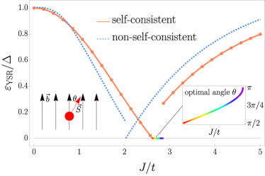
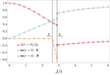
We here examine the impact of self-consistency in a minimal model: a single magnetic moment placed on an s-wave superconductor in the presence of weak magnetic field. Our detailed analysis reveals that even in this simple model the non-selfconsistent approach misses important qualitative physics: while without self-consistency there is only a singular critical value at which the resonance energy equals the Fermi energy, i.e. , the fully self-consistent calculation reveals a critical phase, i.e., a finite interval of values, see Fig. 1. Within this phase the relative angle between the moment and the quantization direction of the superconductor, , rotates continuously from orthogonal () to anti-aligned , see inset of Fig. 1. Beyond the observation that within this region , this transition is also characterized by a high-amplitude magnetization response around the magnetic impurity, as will be discussed in the section “Self-consistent fields”.
Our findings hold particular significance near criticality, where the energy of the YSR states reaches the system’s Fermi energy. Notably, this region is of specific interest in studies investigating the potential emergence of Majorana Zero Modes in similar systems [27, 31].
Model and Method. We a consider the model Hamiltonian:
| (1) |
where
| (2) |
denotes a nearest-neighbor tight-binding Hamiltonian with hopping parameter, , and chemical potential . The Fermionic operators obey the usual anti-commutation relations: . While the derivation of the basic equations is general, we present explicit results for hexagonal lattices. We are motivated by the prevalence of such symmetries in many experimental samples or systems that can be effectively reduced to hexagonal lattice configurations, as demonstrated for NbSe2 in [8]. The Hubbard term in (1),
| (3) |
embodies the onsite attractive () interaction where is the number operator, depicting the electron occupancy at site with spin .
We further incorporate the external magnetic field introducing a Zeeman-term
| (4) |
which breaks spin-rotation symmetry; here , and represents the magnetic field strength. Finally, the magnetic impurity is implemented via
| (5) |
at the lattice site ; denotes the exchange coupling constant for magnetic interactions. A local potential with strength is also foreseen; it accounts, e.g., for an impurity-induced Coulomb interaction. Throughout this study, we adopt the assumption of a classical impurity spin, an approach fundamentally outlined in [2].
To characterize the relative orientation between the local magnetic moment and the uniform magnetic field (chosen to point in the direction), we introduce a spherical parametrization for , described by the polar () and azimuthal () angles:
| (6) |
In the absence of spin-orbit coupling, the system exhibits a residual symmetry under rotations around . Since is not equipped with a dynamics of its own, the azimuthal angle defined in (6) is cyclic. Therefore, subsequently we will discuss only the dependence on the polar angle .
Mean-Field Approximation. In the mean-field approximation, the product of number operators on the same site become:
| (7) |
Here, the averages are given by
| (8) |
Applying these approximations to (3), we obtain the mean-field interaction Hamiltonian:
| (9) |
in which and its inverse denote spin-flip processes.
Solving the self-consistency problem. We now turn our attention to the Bogoliubov-de Gennes (BdG) formalism, which is essential to our investigation. In this framework, we can express the fermionic operators, and , in terms of a new set of quasiparticle operators, and , that diagonalize the Hamiltonian:
| (10) |
The prime symbol on the summation indicates that only states with positive energies are to be considered to ensure unitarity. The Hamiltonian in this formalism is given by:
| (11) |
The ground state energy,
| (12) |
contains three parts, with the last two stemming from the Hartree Fock decomposition. Adopting the transformation (10) and , the previously defined variables are expressed as:
| (13) | |||
| (14) |
The BdG Hamiltonian and the details of our self-consistency problem are delegated to [43].
In every numerical simulation conducted in this study, we explored 2D hexagonal lattices at zero temperature with periodic boundary conditions, having an edge length of cells. Setting and yielded a gap and a density of states at the Fermi level . Throughout this letter, we also employ , resulting in a shift of the continuous spectrum boundary to .
Theoretical consideration. From an analytical perspective, solving the self-consistency problem is notoriously challenging. Consequently, researchers often ignored variations in the field distributions and , assuming that effects stemming from their inhomogeneity are marginal. Following these assumptions, we formulate in this subsection some preliminary theoretical expectations. Intriguingly, as we show in subsequent numerical sections, self-consistency introduces notable changes to the non-selfconsistent scenario.
Resonance energy - perturbative analysis. Assuming homogeneous distributions of and , the analytical results for the resonance energy suggest the following behavior of the in-gap energy [3]:
| (15) |
where , . The resonance energy is measured from the Fermi level , which at equals , and denotes the density of states at . At specific critical valuew, , the energy drops to zero, signaling a QPT at which the spontaneous generation of a local quasiparticle excitation becomes energetically favorable.
In order to estimate the effect of the Zeeman term, embarking on [3], we perform a perturbative analysis referring to the Supplementary [43] for details. We obtain for the leading order correction
| (16) |
which implies a sharp jump as the coupling crosses a critical value . A corresponding jump is also seen in the free energy
| (17) |
To rationalize the result (17), we stipulate that the ground state undergoes a magnetic transition, evidence of which will be presented below: at the net moment exhibits a spin-, while at , it exhibts vanishing electronic spin and no net moment[44, 40]. Therefore, there is no linear response of the ground state energy to and in the latter regime.
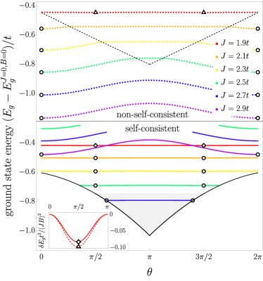
Resonance energy - non-selfconsistent numerics. To go beyond the perturbative limit but still discarding self-consistency, we perform the exact diagonalization numerically, keeping uniform fields and . The result is shown in the upper panel of Fig. 2. Specifically, we display the behavior of the ground state energy as a function of the angle, .
As one would have expected based on (17), the -dependent contribution of the ground-state energy, , at small (with ) the traces are flat (up to quadratic corrections), while at large ( ) they exhibit a cosine shape. A new feature of the numerical solution as compared to (17) is the existence of the transition window , which opens up as rises from zero. In this intermediate regime, for each combination of () there is an angle such that is a flat function for ; see the dashed triangle in Fig. 2.
The evolution of the (non-self-consistent) YSR-resonance, , corresponding to was already shown in Fig. 1: with increasing coupling , the resonance energy splits from the continuum () and moves gradually towards the band center that, however, is ultimately reached only after a sharp jump corresponding to dropping abruptly from to zero.
Ground-state magnetization. The minimum of , , provides the optimal orientation of the impurity spin with respect to the external field . At one infers from Fig. 2 that ; at large coupling, the impurity fully aligns with the external field. At this instance, the local field became large enough to locally break a Cooper pair with the consequence that an electronic spin-1/2 is created. This electronic spin couples linearly to the external magnetic field, which was the rational for explaining Eq. (17).
The situation in the regime requires further attention. Since the system does not couple linearly to , c. f. Eq. (17), one expects that all Cooper pairs have remained intact and, correspondingly, vanishing electronic spin. As illustrated in Fig. 2, inset, the dependency of is indeed of order in , with the expected modulation; for details see [43]. Further, , so that the moment points perpendicular to the quantization axis . Thus the impurity’s effect, i.e. perturbing the condensate, becomes minimal mitigating the destruction of Cooper pairs.
Discussion. Any non-selfconsistent implies a lack of feedback: while the eigenfunctions of gradually deform with increasing impurity strength, the coupling remains unaffected. Therefore, pair breaking does not cost the energy ; consequently, the total energy of the spin-0 state shown in the upper panel of Fig. 2 is too low by an amount as compared to the spin-1/2 state. This artifact is likely to invalidate a non-selfconsistent description of the magnetic phase transition, so that a fully self-consistent treatment is required.
Fully self-consistent numerics. As we demonstrate in this section, full self-consistency changes the scenario significantly because it restores teh energy cost for pair-breaking.
Ground state energy. At weak coupling, i.e. , is nearly constant (spin-0 phase) reproducing the result ignoring self-consistency. At strong coupling, , the total energy exhibits the familiar shape indicating the spin-1/2. Contrasting the non-selfconsistent result, Fig. 2, upper panel, the evolution of with from weak to strong coupling is not monotonous in Fig. 2, lower panel: the spin-1/2 state is lifted in energy as compared to the spin-0 state by an amount indicating the cost of pair-breaking. This extra energy cost manifests as a sharp jump in seen in the critical window in Fig. 2, lower panel, e.g. at and . As a consequence of this extra cost the spin-0 state remains stable even as grows into the critical window; correspondingly the optimal angle stays near and does not jump to as predicted without self-consistency. In fact, upon approaching the angle first increases to values exceeding , c.f. inset of Fig. 1. This implies that the impurity anti-aligns with the external field in order to prevent the Cooper-pair to split. Only when with growing -field the Zeemann-energy eventually overcomes the energy cost for pair breaking does the spin-1/2 ground state emerge.
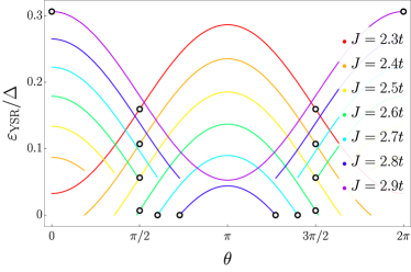
Yu-Shiba-Rusinov resonance energy. The transition from the spin-0 to the spin-1/2 state occurs in a mean-field framework by means of a level crossing. At weak coupling, , the occupied level, i.e. the YSR-resonance, hosts a Cooper pair that is localized near the impurity. At very large coupling, , the Zeemann-energy dominates, so the orbitals are spin-split: one spin-direction is occupied (majority) while the other is empty (minority). The entire scenario is contained in the trace of displayed in Fig. 3: as reaches , the YSR state’s energy reaches the Fermi energy , thus hallmarking the transition [44, 45, 46]; it manifests in the change in local electronic states [44, 45, 46, 19], transport and magnetic properties [47, 13, 48]. The analysis of has revealed the existance of a critical window, , in which moves from to before the spin-1/2 phase with is reached. Upon entering the critical window, , the Cooper pair is at the verge of destruction, which is why the resonance is close to the . It stays there throughout the window until it dissolves, eventually, at leaving the window, i.e.. We therefore witness in Fig. 3 that is pinned to throughout the critical window of values.
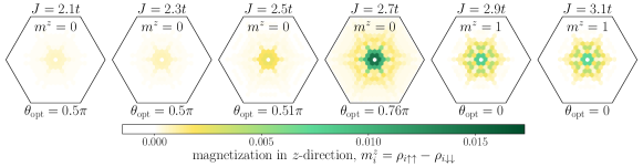
Self-consistent fields. The spatial distribution patterns of self-consistent fields, i.e. particle densities , magnetization , and the order parameter , are experimental observables. We analyze how they reflect the QPT. For additional details, we refer to Supplementary Materials [43].
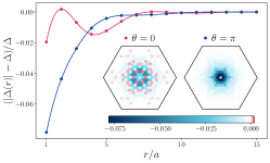
In Fig. 4 we show how the the spatial profile of and vary with the polar angle . When comparing the profiles that all correspond to (spin- state) and (spin-0 state) in Fig. 4 left, the field distribution displays markedly different patterns. (While in this section we plot the spatial distribution of the gap starting from (one cell) from the impurity, the Supplementary Material [43] (Fig. 2) illustrates the discontinuous behavior of at the impurity’s site . Notably, at the point of the QPT, the sign of changes and becomes negative for .)
The distribution of magnetization induced by the local impurity follows a similar trend, as shown in Fig. 4, right. As we observe progressing from to , the critical region reveals itself by a distinct change in the magnetization profile and the total spin polarization . When , i.e. , the magnetization response in the -direction is minimal, which plays a crucial role in the spin-0 phase. Conversely, in the region , where and , the magnetization response is anomalously large, which is evident from the figure corresponding to in Fig. 4 right.
Discussion. Our analysis revealed that self-consistency significantly alters the previously understood non-self-consistent picture. Notably, the destruction of Cooper pairs near criticality is mitigated by the reorientation of the impurity’s magnetic moment, where the angle between the external magnetic field and , denoted as , exceeds . This reorientation reduces the energy of a localized electron experiencing in -direction the effective magnetic field , which is lower than when , at the impurity’s site.
Although a detailed analytical solution to the self-consistent problem is beyond the scope of this letter, in the leading order in , we summarize the significance of self-consistency with the following approximate expressions:
| (18) |
Accordingly, within this critical region of width approximately , we predict
| (19) |
These expressions are derived under the premise that the primary function of self-consistency lies in mitigating Cooper pair breaking, which reveals itself in the abrupt jump in the ground state energy .
We emphasize that in actual superconducting materials, mechanisms other than external magnetic fields may break the spin-rotation symmetry, e.g., a finite density of magnetic impurities or a form of spontaneous symmetry breaking. We expect our results to carry over to these situations. Specifically, the width of the critical region, expressed as in our model, will be replaced by , where quantifies the strength of the symmetry breaking perturbation.
Moreover, in the realm of Shiba chains, we predict that self-consistency is not merely a theoretical nuance but has tangible consequences. We expect that even in the absence of the external field, it could lead to impurity spin reorientations. This becomes particularly critical for chains of impurities, where collective behaviors and interactions significantly alter the system’s characteristics.
In the realm of quantum spins, we expect that the mechanism here reported qualitatively survives: In a certain region of the coupling constants , the expectation value for the impurity’s spin will be negative, i.e., oriented in the direction opposite to the external magnetic field. This orientation will consequently alter the behavior of the in-gap state’s energy, the distribution of the local density of states (LDoS), and the magnetic response.
Conclusion. In this study, we have explored the role of self-consistency in a minimal system featuring a magnetic impurity embedded in an s-wave superconductor subject to weak magnetic field, with a particular focus on the ground state properties and the behavior of Yu-Shiba-Rusinov states. Our analysis reveals that self-consistency leads to qualitatively new effects if the dimensionless coupling, , of the impurity to the superconductor approaches its critical value . Specifically, while the conventional understanding anticipates a singular critical point, , predict a critical phase where , as illustrated in Fig. 1.
There are several promising directions for future research. (i) While our study focuses on a classical magnetic moment of the impurity, testing our results in the quantum case is of great interest. (ii) In the context of Majorana bound states, investigating the effect of self-consistency in YSR-spin chains and the associated quantum phase transitions in YSR bands opens new avenues for exploration. (iii) Finally, on the experimental front, detailed studies of magnetization and LDoS spatial distributions, as well as the behavior of YSR peaks as functions of , , chemical potential , magnetic field strength , and electron density , would greatly augment our understanding of these complex systems. With an eye on the latter, we mention that a magnetic tip as is used in STM experiments can act as a local magnetic impurity. Since the distance between the superconducting substrate and the tip can be adjusted to alter the coupling strength , the phase-transition should be amenable to STM measurements, at least in principle.
Acknowledgements.
E.S.A. and F. E. are grateful to I. Burmistrov for useful discussions and collaborations on related research. E.S.A. acknowledges useful discussions and constructive criticism from P. Brouwer, S.S. Babkin, D.E. Kiselev, and K.G. Nazaryan. The Gauss Centre for Supercomputing e.V. is acknowledged for providing computational resources on SuperMUC-NG at the Leibniz Supercomputing Centre under the Project ID pn36zo. E.S.A and F. E. acknowledge support by the Deutsche Forschungsgemeinschaft (DFG, German Research Foundation) within Project-ID 314695032 – SFB 1277 (project A03 and IRTG) - and by the DFG projects EV30/14-1 and EV30/11-2.References
- Yu [1965] L. Yu, Bound state in superconductors with paramagnetic impurities, Wu Li Hsueh Pao (China) Supersedes Chung-Kuo Wu Li Hsueh For English translation see Chin. J. Phys. (Peking) (Engl. Transl.) 21, (1965).
- Shiba [1968] H. Shiba, Classical Spins in Superconductors, Progress of Theoretical Physics 40, 435 (1968).
- Rusinov [1968] A. I. Rusinov, Jetp lett., JETP Letters 9 (1968).
- Yazdani et al. [1997] A. Yazdani, B. A. Jones, C. P. Lutz, M. F. Crommie, and D. M. Eigler, Probing the local effects of magnetic impurities on superconductivity, Science 275, 1767 (1997).
- Ruby et al. [2015a] M. Ruby, F. Pientka, Y. Peng, F. von Oppen, B. W. Heinrich, and K. J. Franke, Tunneling processes into localized subgap states in superconductors, Phys. Rev. Lett. 115, 087001 (2015a).
- Ménard et al. [2015] G. Ménard, S. Guissart, C. Brun, et al., Coherent long-range magnetic bound states in a superconductor, Nature Physics 11, 1013 (2015).
- Yang et al. [2020] X. Yang, Y. Yuan, Y. Peng, E. Minamitani, L. Peng, J.-J. Xian, W.-H. Zhang, and Y.-S. Fu, Observation of short-range yu-shiba-rusinov states with threefold symmetry in layered superconductor 2h-nbse2, Nanoscale 12, 8174 (2020).
- Liebhaber et al. [2020] E. Liebhaber, S. Acero González, R. Baba, G. Reecht, B. W. Heinrich, S. Rohlf, K. Rossnagel, F. von Oppen, and K. J. Franke, Yu–shiba–rusinov states in the charge-density modulated superconductor nbse2, Nano Letters 20, 339 (2020), pMID: 31842547.
- Odobesko et al. [2023] A. Odobesko, R. L. Klees, F. Friedrich, E. M. Hankiewicz, and M. Bode, Boosting the stm’s spatial and energy resolution with double-functionalized probe tips, arXiv preprint arXiv:2303.02406 (2023).
- Ji et al. [2008] S.-H. Ji, T. Zhang, Y.-S. Fu, X. Chen, X.-C. Ma, J. Li, W.-H. Duan, J.-F. Jia, and Q.-K. Xue, High-resolution scanning tunneling spectroscopy of magnetic impurity induced bound states in the superconducting gap of pb thin films, Phys. Rev. Lett. 100, 226801 (2008).
- Ruby et al. [2016] M. Ruby, Y. Peng, F. von Oppen, B. W. Heinrich, and K. J. Franke, Orbital picture of yu-shiba-rusinov multiplets, Phys. Rev. Lett. 117, 186801 (2016).
- Huang et al. [2020a] H. Huang, C. Padurariu, J. Senkpiel, et al., Tunnelling dynamics between superconducting bound states at the atomic limit, Nature Physics 16, 1227 (2020a).
- Huang [2021] H. Huang, Yu-Shiba-Rusinov states and the Josephson effect, Ph.D. thesis, Max Planck Institute for Solid State Research (2021).
- Küster et al. [2021] F. Küster, A. M. Montero, F. S. M. Guimaraes, S. Brinker, S. Lounis, S. S. P. Parkin, et al., Correlating josephson supercurrents and shiba states in quantum spins unconventionally coupled to superconductors, Nature Communications 12, 1108 (2021).
- Trahms et al. [2023] M. Trahms, L. Melischek, J. F. Steiner, et al., Diode effect in josephson junctions with a single magnetic atom, Nature 615, 628 (2023).
- Kezilebieke et al. [2019] S. Kezilebieke, R. Žitko, M. Dvorak, T. Ojanen, and P. Liljeroth, Observation of coexistence of yu-shiba-rusinov states and spin-flip excitations, Nano Letters 19, 4614 (2019), pMID: 31251066.
- Farinacci et al. [2018] L. Farinacci, G. Ahmadi, G. Reecht, M. Ruby, N. Bogdanoff, O. Peters, B. W. Heinrich, F. von Oppen, and K. J. Franke, Tuning the coupling of an individual magnetic impurity to a superconductor: Quantum phase transition and transport, Phys. Rev. Lett. 121, 196803 (2018).
- Huang et al. [2020b] H. Huang, R. Drost, J. Senkpiel, et al., Quantum phase transitions and the role of impurity-substrate hybridization in yu-shiba-rusinov states, Communications Physics 3, 199 (2020b).
- Huang et al. [2020c] H. Huang, R. Drost, J. Senkpiel, et al., Quantum phase transitions and the role of impurity-substrate hybridization in yu-shiba-rusinov states, Communications Physics 3, 199 (2020c).
- Kezilebieke et al. [2018] S. Kezilebieke, M. Dvorak, T. Ojanen, and P. Liljeroth, Coupled yu–shiba–rusinov states in molecular dimers on nbse2, Nano Letters 18, 2311 (2018), pMID: 29533636.
- Malavolti et al. [2018] L. Malavolti, M. Briganti, M. Hänze, G. Serrano, I. Cimatti, G. McMurtrie, E. Otero, P. Ohresser, F. Totti, M. Mannini, R. Sessoli, and S. Loth, Tunable spin–superconductor coupling of spin 1/2 vanadyl phthalocyanine molecules, Nano Letters 18, 7955 (2018), pMID: 30452271.
- Ruby et al. [2018] M. Ruby, B. W. Heinrich, Y. Peng, F. von Oppen, and K. J. Franke, Wave-function hybridization in yu-shiba-rusinov dimers, Phys. Rev. Lett. 120, 156803 (2018).
- Friedrich et al. [2021] F. Friedrich, R. Boshuis, M. Bode, and A. Odobesko, Coupling of yu-shiba-rusinov states in one-dimensional chains of fe atoms on nb(110), Phys. Rev. B 103, 235437 (2021).
- Choy et al. [2011a] T.-P. Choy, J. M. Edge, A. R. Akhmerov, and C. W. J. Beenakker, Majorana fermions emerging from magnetic nanoparticles on a superconductor without spin-orbit coupling, Phys. Rev. B 84, 195442 (2011a).
- Choy et al. [2011b] T.-P. Choy, J. M. Edge, A. R. Akhmerov, and C. W. J. Beenakker, Majorana fermions emerging from magnetic nanoparticles on a superconductor without spin-orbit coupling, Phys. Rev. B 84, 195442 (2011b).
- Martin and Morpurgo [2012] I. Martin and A. F. Morpurgo, Majorana fermions in superconducting helical magnets, Phys. Rev. B 85, 144505 (2012).
- Nadj-Perge et al. [2013] S. Nadj-Perge, I. K. Drozdov, B. A. Bernevig, and A. Yazdani, Proposal for realizing majorana fermions in chains of magnetic atoms on a superconductor, Phys. Rev. B 88, 020407 (2013).
- Braunecker and Simon [2013] B. Braunecker and P. Simon, Interplay between classical magnetic moments and superconductivity in quantum one-dimensional conductors: Toward a self-sustained topological majorana phase, Phys. Rev. Lett. 111, 147202 (2013).
- Klinovaja et al. [2013] J. Klinovaja, P. Stano, A. Yazdani, and D. Loss, Topological superconductivity and majorana fermions in rkky systems, Phys. Rev. Lett. 111, 186805 (2013).
- Vazifeh and Franz [2013] M. M. Vazifeh and M. Franz, Self-organized topological state with majorana fermions, Phys. Rev. Lett. 111, 206802 (2013).
- Pientka et al. [2013] F. Pientka, L. I. Glazman, and F. von Oppen, Topological superconducting phase in helical shiba chains, Phys. Rev. B 88, 155420 (2013).
- Pientka et al. [2014] F. Pientka, L. I. Glazman, and F. von Oppen, Unconventional topological phase transitions in helical shiba chains, Phys. Rev. B 89, 180505 (2014).
- Li et al. [2014] J. Li, H. Chen, I. K. Drozdov, A. Yazdani, B. A. Bernevig, and A. H. MacDonald, Topological superconductivity induced by ferromagnetic metal chains, Phys. Rev. B 90, 235433 (2014).
- Reis et al. [2014] I. Reis, D. J. J. Marchand, and M. Franz, Self-organized topological state in a magnetic chain on the surface of a superconductor, Phys. Rev. B 90, 085124 (2014).
- Röntynen and Ojanen [2015] J. Röntynen and T. Ojanen, Topological superconductivity and high chern numbers in 2d ferromagnetic shiba lattices, Phys. Rev. Lett. 114, 236803 (2015).
- Nadj-Perge et al. [2014] S. Nadj-Perge, I. K. Drozdov, J. Li, H. Chen, S. Jeon, J. Seo, A. H. MacDonald, B. A. Bernevig, and A. Yazdani, Observation of majorana fermions in ferromagnetic atomic chains on a superconductor, Science 346, 602 (2014).
- Ruby et al. [2015b] M. Ruby, F. Pientka, Y. Peng, F. von Oppen, B. W. Heinrich, and K. J. Franke, End states and subgap structure in proximity-coupled chains of magnetic adatoms, Phys. Rev. Lett. 115, 197204 (2015b).
- Pawlak et al. [2016] R. Pawlak, M. Kisiel, J. Klinovaja, et al., Probing atomic structure and majorana wavefunctions in mono-atomic fe chains on superconducting pb surface, npj Quantum Information 2, 16035 (2016).
- Schneider et al. [2022] L. Schneider, P. Beck, J. Neuhaus-Steinmetz, et al., Precursors of majorana modes and their length-dependent energy oscillations probed at both ends of atomic shiba chains, Nature Nanotechnology 17, 384 (2022).
- Salkola et al. [1997] M. I. Salkola, A. V. Balatsky, and J. R. Schrieffer, Spectral properties of quasiparticle excitations induced by magnetic moments in superconductors, Phys. Rev. B 55, 12648 (1997).
- Flatté and Byers [1997] M. E. Flatté and J. M. Byers, Local electronic structure of defects in superconductors, Phys. Rev. B 56, 11213 (1997).
- Schlottmann [1976] P. Schlottmann, Spatial variations of the order parameter in superconductors containing a magnetic impurity, Phys. Rev. B 13, 1 (1976).
- Andriyakhina et al. [2024] E. S. Andriyakhina, S. L. Khortsev, and F. Evers, Supplementary material for “fermi-level pinning of yu-shiba-rusinov states in weak magnetic field” (2024).
- Sakurai [1970] A. Sakurai, Comments on Superconductors with Magnetic Impurities, Progress of Theoretical Physics 44, 1472 (1970).
- Matsuura [1977] T. Matsuura, The Effects of Impurities on Superconductors with Kondo Effect, Progress of Theoretical Physics 57, 1823 (1977), https://academic.oup.com/ptp/article-pdf/57/6/1823/5461826/57-6-1823.pdf .
- Sakai et al. [1993] O. Sakai, Y. Shimizu, H. Shiba, and K. Satori, Numerical renormalization group study of magnetic impurities in superconductors. ii. dynamical excitation spectra and spatial variation of the order parameter, Journal of the Physical Society of Japan 62, 3181 (1993).
- Ptok et al. [2017] A. Ptok, S. Głodzik, and T. Domański, Yu-shiba-rusinov states of impurities in a triangular lattice of with spin-orbit coupling, Phys. Rev. B 96, 184425 (2017).
- Lopez-Bezanilla and Lado [2019] A. Lopez-Bezanilla and J. L. Lado, Defect-induced magnetism and yu-shiba-rusinov states in twisted bilayer graphene, Phys. Rev. Mater. 3, 084003 (2019).
Supplementary Material for
“Fermi-Level Pinning of Yu-Shiba-Rusinov States in Weak Magnetic Field”
A Self-Consistency Problem
This section delineates the details of the self-consistency problem we solve in the main text. After we perform the Bogoliubov-de Gennes transformation, the BdG Hamiltonian’s matrix elements, in the basis , become:
| (A.20) |
Here, is defined as . The above equations culminate in the following eigenvalue problem for our system:
| (A.21) |
that are complimented by the self-consistency conditions
| (A.22) |
The solution to this problem will provide us with insights into the behavior of our system under the conditions described.
Throughout this work, we consider hexagonal samples with edge length lattice constants. Periodic boundary conditions were applied. The stability of our solutions was verified against different random initial conditions, assuming convergence when the maximal difference of the chemical potential and the fields and at any lattice site between two consecutive iterations is less than a specified tolerance level , set at . The robustness of our solutions was further evaluated by varying and comparing the results.
B Analytical Solution Neglecting Self-Consistency
In this section, we analytically derive the effect a weak magnetic field has on the energy of the Yu-Shiba-Rusinov state. For simplicity in our narrative, we will assume that (the non-magnetic part of the local potential) is zero, cf. Eq. (5) of the main text.
We begin by formulating the equation to determine the wave-functions and energies
| (B.23) |
Here, represents the deviation of the energy spectrum of the electrons in the lattice from the Fermi level , and we assumed a homogeneous pairing potential .
For analytical convenience, we consider a rotated basis in which the magnetic moment of the impurity points in the direction. This is accomplished by introducing the rotation matrix , which, in the basis , reads as
| (B.24) |
Upon applying this rotation to our formulation in Eq. (B.23), we immediately note that only the component arising from the homogeneous magnetic field is altered. In the rotated basis, we find
| (B.25) |
In the subsequent analysis, we will incorporate the magnetic field perturbatively. To that end, let us consider the unperturbed problem,
| (B.26) |
Switching to momentum space, we immediately obtain
| (B.27) |
Upon reverting back to real space and seeking the solution at the impurity’s site (), we are presented with the following matrix equation:
| (B.28) |
Here, denotes the density of states at the Fermi energy. Noteworthy, the magnetic impurity influences the above-the-gap continuum of states by altering the plane waves into their combinations, such that . Here, is the wave-function corresponding to . Focusing on the in-gap state, where , the above equation yields (for ):
| (B.29) |
and for
| (B.30) |
In the above expressions, is the normalization constant that ensures . It is given by
| (B.31) |
If we now perturbatively incorporate the magnetic field as described by Eq. (B.25), we readily find:
| (B.32) |
In order to calculate the lowest order correction to the free energy , we recall that this correction can be conveniently formulated as
| (B.33) |
where and are the spin-resolved densities induced by the magnetic impurity in the absence of a magnetic field . Eq. (B.33) suggests that the correction involves a Zeeman coupling of the magnetic field to the impurity-induced magnetization , which assumes the value when and when .
C Ground State Energy in Weak Coupling Regime
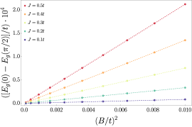
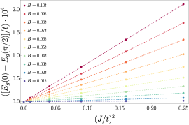
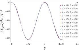
In this section, we present numerical results for the weak-coupling regime, where the net electronic spin is and, consequently, the ground state energy remains independent of at the first order, cf. Eq. (B.33). Assuming a homogeneous gap , a filling factor of , and , we explored the variation of the coupling strength and the magnitude of the external field . This analysis revealed a dependence of , as illustrated in the rightmost plot of Fig. S1. To ascertain the parametric dependence of the amplitude of this harmonic, we examined with respect to both and . Our analysis suggests a quadratic dependence on both and , i.e., with some constant . For clarity of presentation, the behavior of as a function of and is depicted in the left and middle figures of Fig. S1. To further substantiate our claim, we present the rightmost plot in Fig. S1, that illustrates the evolution of normalized by , which also suggests that the amplitude of is directly proportional to . We would like to emphasize that to render the scales dimensionless, in Fig. S1, we normalized all quantities with respect to the hopping amplitude . Nonetheless, the appropriate dimensionless parameters should be and , which depend not only on , but on the filling factor as well.
D Order Parameter and Magnetic Moment at the Impurity Site
This section presents typical plots, illustrated in Fig. S2, of the behavior of the local pairing potential (normalized to the homogeneous value far from the impurity) and the magnetic polarization at the impurity’s site () as functions of the impurity-to-substrate coupling constant .
Two critical values, and , delineate the region where the YSR state’s energy matches the Fermi level and the impurity’s magnetic moment points in the opposite direction to the external magnetic field, forming an angle , cf. Fig. 1 of the main text. These thresholds are indicated by vertical dashed lines. It becomes further evident from this plot that within the region , the magnetic moment of the impurity on the -axis (axis of the external magnetic field) assumes negative values. After crossing , both , , and exhibit abrupt jumps corresponding to the local destruction of Cooper pairs and alteration of the Fermi sea structure.
We note that , which aligns with our analytical predictions, see Eq. (18) of the main text.