Fock’s dimer model on the Aztec diamond

Abstract

We consider the dimer model on the Aztec diamond with Fock’s weights, which is gauge equivalent to the model with any choice of positive weight function. We prove an explicit, compact formula for the inverse Kasteleyn matrix, thus extending numerous results in the case of periodic graphs. We also show an explicit product formula for the partition function; as a specific instance of the genus 0 case, we recover Stanley’s formula [Pro97, Yan91]. We then use our explicit formula for the inverse Kasteleyn matrix to recover, in a simple way, limit shape results; we also obtain new ones. In doing so, we extend the correspondence between the limit shape and the amoeba of the corresponding spectral curve of [BB23] to the case of non-generic weights.

1 Introduction

We consider the dimer model on the Aztec diamond with Fock’s weights [Foc15, BCdT23a]. Our first main result is an explicit expression for the inverse Kasteleyn matrix, which only uses theta functions, prime forms and local functions in the kernel of the associated Kasteleyn operator. We also prove that any dimer model on the Aztec diamond is gauge equivalent to a dimer model with Fock’s weights, thus showing that we actually treat the dimer model on the Aztec diamond in full generality. Next, building on an idea of Propp [Pro97], we prove an induction formula for the partition function, showing that it admits a product form; as a specific case, we recover Stanley’s celebrated formula [Yan91]. Finally, we use our explicit formula for the inverse Kasteleyn matrix to recover and extend, in a simple way, results on limit shapes in genus 0, 1, and higher, generalizing the geometric correspondence between the limit shape of the Aztec diamond for periodic weights and the amoeba of the corresponding spectral curve proven by Berggren and Borodin [BB23] under some technical assumptions, which are now lifted.

Let us now be more specific, and give some historical background. This paper aims at, in some sense, closing a long history of formulas for the inverse Kasteleyn matrix of the dimer model on the Aztec diamond. This was initiated in [Hel00] in the case of uniform weights. Then, in [CJY15], Chhita, Johansson and Young consider the case where vertical and horizontal dominos have different weights, also known as 1-periodic weights; their proof consists in connecting dimer configurations to particle systems together with a direct check of their guessed formula. Next in [CY14], Chhita and Young treat the case of 1-periodic weights with a possible volume penalization, and 2-periodic weights; to prove their result, the authors use generating functions. The 1-periodic weights with volume penalization is then generalized in [BBC⁺17] using the connection to Schur processes. In [CJ16] Chhita and Johannsson again consider 2-periodic weights; they prove a simplification of the formula of [CY14], compute asymptotics of the inverse and limit shapes, in particular they discuss the arctic curves separating the various phases given by an algebraic curve of degree 8. In [DK21], Duits and Kuijlaars propose a different approach for the 2-periodic weights of [CY14] using non intersecting lattice paths and matrix valued orthogonal polynomials; allowing them to compute finer asymptotics using an associated Riemann-Hilbert problem. A new approach, involving block Toepliz matrices and the Wiener-Hopf factorization is proposed in [BD19]; it is then extended to $2\times k$-periodic weights in [Ber21]; in particular, the authors give a rigorous proof of the arctic curves derived in [DFSG14]. In [BD23], Borodin and Duits introduce biased $2\times 2$ periodic weights; two specific cases are the 1-periodic weights of [CJY15] and the 2-periodic ones of [CY14]; the method used is that of block Toepliz matrices and Wiener-Hopf factorization. This approach culminates in the paper [BB23], where the authors consider generic $k\times l$-periodic weights, where generic means that the underlying spectral curve has maximal genus. Note that weights of the above $k\times l$ and $2\times k$ models can be specified so as to recover the 2-periodic weights of [CY14], but then the weights are not generic as assumed in the latter papers, so that the setting is actually different.

Our first main result, Theorem 13, encompasses all of the above cases. Here is the setting, see Sections 2.1, 2.2 for more details. Consider an M-curve $\Sigma$ of genus $g$, with a distinguished real component $A_{0}$, and a real element $t$ of the Jacobian variety $\mathrm{Jac}(\Sigma)$. Denote by $\theta$ the associated Riemann theta function and by $E$ the prime form. Consider an Aztec diamond $\mathsf{A}_{n}$ of size $n$, with its set of oriented train-tracks $\vec{\mathscr{T}}_{n}$ naturally split into four, and let ${\bm{\alpha}}=(\alpha_{j})_{j=1}^{n}$, ${\bm{\beta}}=(\beta_{j})_{j=1}^{n}$, ${\bm{\gamma}}=(\gamma_{j})_{j=1}^{n}$, ${\bm{\delta}}=(\delta_{j})_{j=1}^{n}$ be the associated angles on $A_{0}$ satisfying the cyclic order conditions ${\bm{\alpha}}<{\bm{\gamma}}<{\bm{\beta}}<{\bm{\delta}}$. Suppose that edges of the Aztec diamond are assigned Fock’s weights [Foc15, BCdT23a], meaning that, for every edge $\mathsf{w}\mathsf{b}$ with train-track angles $\alpha,\beta$, the corresponding coefficient of the Kasteleyn matrix $\mathsf{K}$ is given by:

$$\mathsf{K}_{\mathsf{w},\mathsf{b}}=\frac{E(\alpha,\beta)}{\theta(t+\mathbf{d}(\mathsf{f}))\theta(t+\mathbf{d}(\mathsf{f}^{\prime}))},$$

where $\mathsf{f},\mathsf{f}^{\prime}$ are the dual faces adjacent to $\mathsf{w}\mathsf{b}$, and $\mathbf{d}$ is the discrete Abel map. In Proposition 11, we prove that all dimer models on the Aztec diamond can be re-parameterized using Fock’s weights. Then, Theorem 13 can loosely be stated as follows.

Theorem 1.

For every pair $(\mathsf{b},\mathsf{w})$ of black and white vertices of $\mathsf{A}_{n}$, the coefficient $(\mathsf{b},\mathsf{w})$ of the inverse Kasteleyn matrix is explicitly given by

$$\mathsf{K}^{-1}_{\mathsf{b},\mathsf{w}}=\frac{1}{(2\pi i)^{2}}\frac{1}{\theta(p)}\int_{\mathscr{C}_{2}}\int_{\mathscr{C}_{1}}\frac{\theta(p+(v-u))}{E(u,v)}g_{\mathsf{b},0}(u)g_{0,\mathsf{w}}(v)\prod_{j=1}^{n}\frac{E(\beta_{j},u)}{E(\delta_{j},u)}\frac{E(\delta_{j},v)}{E(\beta_{j},v)}+\\ -\mathbb{I}_{\{\mathsf{b}\text{ right of }\mathsf{w}\}}\frac{1}{2\pi i}\int_{\mathscr{C}_{2}}g_{\mathsf{b},\mathsf{w}}(v),$$ (1)

where $\mathscr{C}_{1}$, $\mathscr{C}_{2}$ are closed contours on $\Sigma$ used to integrate over $u$ and $v$, defined in Section 3.2; $p=\sum\limits_{j=1}^{n}(\delta_{j}-\beta_{j})-t-\mathbf{d}(0)$, and $g$ is the form in the kernel of the Kasteleyn matrix introduced in [BCdT23a], see also Equation (13).

Note that to recover known results on the Aztec diamond requires to identify the associated weights in Fock’s form. We do this explicitly in Section 2.3 in the genus 0 case, which includes Stanley’s weights [Pro97, Yan91], and in the genus 1 case, which includes the biased $2\times 2$ periodic case of [BD23].

Our next result, Theorem 16, proves that the partition function admits a product form. Denote by $Z_{n}({\bm{\alpha}},{\bm{\beta}},{\bm{\gamma}},{\bm{\delta}};d)$ the partition function of the Aztec diamond $\mathsf{A}_{n}$ of size $n$, with train-track angle parameters ${\bm{\alpha}},{\bm{\beta}},{\bm{\gamma}},{\bm{\delta}}$, and value $d$ for the Abel map at the vertex with coordinates $(0,0)$. Then, Theorem 16 can be stated as follows.

Theorem 2.

For every $n\geq 1$, the partition function of the Aztec diamond $\mathsf{A}_{n}$ with Fock’s weights satisfies the following recurrence:

$$Z_{n}({\bm{\alpha}},{\bm{\beta}},{\bm{\gamma}},{\bm{\delta}};d) \cdot\prod_{f\in\mathrm{odd}_{n}}\frac{\theta(t+\mathbf{d}(\mathsf{f}))}{\theta(t+\mathbf{d}(\mathsf{f})+\alpha+\beta-\gamma-\delta)}\prod_{\mathsf{f}\in\mathrm{bry}_{n}}\theta(t+\mathbf{d}(\mathsf{f}))=$$

$$=Z_{n-1} ((\alpha_{j})_{j=1}^{n-1},(\beta_{j})_{j=2}^{n},(\gamma_{j})_{j=1}^{n-1},(\delta_{j})_{j=2}^{n};d+\beta_{1}-\delta_{1})\cdot\Bigl{[}\prod_{j=1}^{n}\ |E(\alpha_{j},\beta_{j})E(\gamma_{j},\delta_{j})|\Bigr{]},$$

with the convention that $Z_{0}=1$.

As specific instances of the genus 0 case, we re-derive that the number of domino tilings of the Aztec diamond is $2^{\frac{n(n+1)}{2}}$, see Remark 19 after Corollary 18, and Stanley’s formula [Pro97, Yan91], see Corollary 20.

We then explain in Lemma 23 that the formula for $\mathsf{K}^{-1}$ for the finite Aztec diamond can be extended in a natural way to an operator $\mathsf{J}$ on an infinite minimal graph containing the Aztec diamond as a subgraph, introduced in [Spe07] and this formula is an inverse for the Fock Kasteleyn operator on this infinite graph. This operator $\mathsf{J}$ does not belong to the family of inverses defined in [BCdT23a]. It nevertheless carries a probabilistic meaning and allows to define a Gibbs measure on dimer configurations of this infinite graph, as stated in Proposition 25. Here is a less formal version:

Proposition 3.

The determinantal process on edges given by $\mathsf{J}$ defines a Gibbs measure on the dimer configurations of the infinite minimal graph, which is supported on configurations which are frozen outside the Aztec region and whose marginals on the edges of the Aztec region coincide with the Boltzmann measure given by Fock’s weights.

The slope in the frozen region is not constant. The operator $\mathsf{J}$ is the first inverse on an infinite minimal graph for which the corresponding probability measure exhibits different phases (solid/liquid/gas) depending on the location on the same infinite graph.

We end this paper with a section with application to the computation of limit shapes for the Aztec diamond with weights coming from surfaces of genus 0, 1 or higher. We give in particular a short derivation of the arctic ellipse theorem for 1-periodic weights [JPS98, Joh02]. We also explain how to extend results by Berggren and Borodin from [BB23] obtained under some technical assumption to a more general context, see also the forthecoming paper [BBS].

Outline of the paper

• In Section 2, we recall the definition of the Aztec diamond graph, and give the necessary geometric definitions to define Fock’s weights for the dimer model. We then discuss some known examples which fit this framework in genus 0 and 1. Proposition 11 establishes that Fock’s weights are gauge equivalent to any choice of positive weights on the edges.

• In Section 3, we state and give a proof of Theorem 13 giving a compact, explicit formula for the inverse Kasteleyn matrix.

• Section 4 is devoted to results about the partition function of the dimer model. It contains the statement and the proof of Theorem 16 showing a product formula for the partition function. Application to the genus 0 case and Stanley’s formula [Pro97, Yan91] are given.

• In Section 5, we discuss the extension of $\mathsf{K}^{-1}$ to an infinite minimal graph. Lemma 23 gives the structure of this inverse, and Proposition 25 describes the corresponding Gibbs measure.

• Section 6 is a discussion of applications of the formula for $\mathsf{K}^{-1}$ to derive limit shapes and limit of local statistics in the thermodynamical limit, recovering and extending several well-known results on the topic.

Acknowledgments

We thank Tomas Berggren for interesting discussions about the dimer model on the Aztec diamond and for explaining some technical details of [BB23]. The authors are partially supported by the DIMERS project ANR-18-CE40-0033 funded by the French National Research Agency. Part of this research was performed while the first author was visiting the Institute for Pure and Applied Mathematics (IPAM), which is supported by the National Science Foundation (Grant No. DMS-1925919).

2 Definitions and first result

This section is devoted to introducing and motivating the framework of this paper. In Section 2.1, we define the dimer model on the Aztec diamond, and in Section 2.2 we introduce Fock’s weights [Foc15, BCdT23a]. Then, in Section 2.3 we explicitly treat the genus 0, resp. genus 1, case and prove how to recover Stanley’s weights [Pro97, Yan91], resp. the biased $2\times 2$ periodic weights of Borodin-Duits [BD23]. Finally, in Section 2.4, we prove that all dimer models on the Aztec diamond can be parameterized using Fock’s weights, implying that we actually study the most general setting of the dimer model on the Aztec diamond.

2.1 Dimer model on the Aztec diamond

Aztec diamond.

The Aztec diamond of size $n$, denoted by $\mathsf{A}_{n}=(\mathsf{V}_{n},\mathsf{E}_{n})$, is a subgraph of $\mathbb{Z}^{2}$ rotated by $\pi/4$ made of $n$ rows and $n$ columns, see Figure 1. This graph is bipartite and the set of vertices $\mathsf{V}_{n}$ is naturally split into black and white: $\mathsf{V}_{n}=\mathsf{B}_{n}\sqcup\mathsf{W}_{n}$.

\begin{overpic}[width=170.71652pt]{fig_Aztec.pdf} \put(-6.0,11.0){\scriptsize$\alpha_{1}$} \put(-6.0,22.0){\scriptsize$\beta_{1}$} \put(8.0,-4.0){\scriptsize$\gamma_{1}$} \put(21.0,-5.0){\scriptsize$\delta_{1}$} \put(-6.0,32.0){\scriptsize$\alpha_{2}$} \put(-6.0,43.0){\scriptsize$\beta_{2}$} \put(32.0,-4.0){\scriptsize$\gamma_{2}$} \put(43.0,-5.0){\scriptsize$\delta_{2}$} \put(-6.0,55.0){\scriptsize$\alpha_{3}$} \put(-6.0,66.0){\scriptsize$\beta_{3}$} \put(53.0,-4.0){\scriptsize$\gamma_{3}$} \put(64.0,-5.0){\scriptsize$\delta_{3}$} \put(-6.0,77.0){\scriptsize$\alpha_{4}$} \put(-6.0,88.0){\scriptsize$\beta_{4}$} \put(75.0,-4.0){\scriptsize$\gamma_{4}$} \put(86.0,-5.0){\scriptsize$\delta_{4}$} \end{overpic}

Figure 1: Aztec diamond $\mathsf{A}_{n}$ with $n=4$. The diamond graph $\mathsf{A}^{\diamond}_{n}$ is represented with light grey lines, the dual vertices with blue circles, and the four families of oriented train-tracks in red. This figure also sets the notation for the angles ${\bm{\alpha}}=(\alpha_{j})_{j=1}^{n},\dots,{\bm{\delta}}=(\delta_{j})_{j=1}^{n}$ assigned to train-tracks.

The set of faces of $\mathsf{A}_{n}$, denoted by $\mathsf{F}_{n}$, consists of the inner faces and the boundary faces, where the latter correspond to all faces of the rotated $\mathbb{Z}^{2}$ adjacent to the boundary of $\mathsf{A}_{n}$. To every face of $\mathsf{F}_{n}$, one assigns a vertex generically denoted by $\mathsf{f}$; it can be seen as a vertex of the dual graph of $\mathsf{A}_{n}$ modified along the boundary, see Figure 1 (small blue circles), hence $\mathsf{f}$ will be referred to as face or dual vertex.

The Aztec diamond $\mathsf{A}_{n}$ comes with a natural coordinate system: the dual vertex on the bottom left is the origin $0=(0,0)$, every white vertex can be written as $\mathsf{w}=(\mathsf{w}_{x},\mathsf{w}_{y})$, with $\mathsf{w}_{x}\in\{0,2,\dots,2n\}$, $\mathsf{w}_{y}\in\{1,3,\dots,2n-1\}$, every black vertex can be written as $\mathsf{b}=(\mathsf{b}_{x},\mathsf{b}_{y})$, with $\mathsf{b}_{x}\in\{1,3,\dots,2n-1\}$, $\mathsf{b}_{y}\in\{0,2,\dots,2n\}$, every dual vertex $\mathsf{f}=(\mathsf{f}_{x},\mathsf{f}_{y})$ either has both even coordinates, or both odd coordinates.

The vertex set of the diamond graph $\mathsf{A}^{\diamond}_{n}$ consists of the dual vertices of $\mathsf{F}_{n}$ and of the vertices of $\mathsf{V}_{n}$, its edges are obtained by joining every vertex of $\mathsf{F}_{n}$ to the vertices of $\mathsf{V}_{n}$ on the boundary of the face it corresponds to, see Figure 1 (light grey); the diamond graph is made of quadrilaterals. A train-track of $\mathsf{A}_{n}$ is a maximal path crossing edges of the diamond graph so that when it enters a quadrilateral, it exits through the opposite side. Since the graph $\mathsf{A}_{n}$ is bipartite, each train-track has a natural orientation such that white, resp. black, vertices of $\mathsf{A}_{n}$, are on its left, resp. right; we let $\vec{\mathscr{T}}_{n}$ denote the set of oriented train-tracks, see Figure 1 (red). Train-tracks of $\vec{\mathscr{T}}_{n}$ come in four families: two sets of horizontal train-tracks with left-to-right or right-to-left orientation, and two sets of vertical train-tracks with bottom-to-top or top-to-bottom orientation.

Dimer model.

A dimer configuration of $\mathsf{A}_{n}$ is a subset $\mathsf{M}$ of edges such that each vertex of $\mathsf{A}_{n}$ is incident to exactly one edge of $\mathsf{M}$; we let $\mathscr{M}(\mathsf{A}_{n})$ denote the set of dimer configurations of $\mathsf{A}_{n}$. Assume a positive weight function $\nu$ is assigned to edges of $\mathsf{A}_{n}$. The dimer Boltzmann measure, denoted by $\mathbb{P}$, is the probability measure on $\mathscr{M}(\mathsf{A}_{n})$ defined by

$$\forall\,\mathsf{M}\in\mathscr{M}(\mathsf{A}_{n}),\quad\mathbb{P}(\mathsf{M})=\frac{\nu(\mathsf{M})}{Z(\nu)},$$

where $\nu(\mathsf{M})=\prod_{\mathsf{e}\in\mathsf{M}}\nu_{e}$, and $Z(\nu)=\sum_{\mathsf{M}\in\mathscr{M}(\mathsf{A}_{n})}\nu(M)$ is the normalizing constant known as the partition function.

Suppose that we have two positive weight functions $\nu,\tilde{\nu}$ assigned to edges of $\mathsf{A}_{n}$. The corresponding dimer models are said to be gauge equivalent [KOS06], if there exists a function $\psi$ defined on $\mathsf{V}_{n}$ such that, for every edge $\mathsf{w}\mathsf{b}$ of $\mathsf{E}_{n}$, we have $\tilde{\nu}_{\mathsf{w}\mathsf{b}}=\psi(\mathsf{w})\nu_{\mathsf{w}\mathsf{b}}\psi(\mathsf{b})$. Two gauge equivalent dimer models yield the same dimer Boltzmann measure. An equivalent useful way of defining gauge equivalence is the following: consider an inner face $\mathsf{f}$ of degree $2k$ of $\mathsf{A}_{n}$, and denote by $\mathsf{w}_{1},\mathsf{b}_{1},\dots,\mathsf{w}_{k},\mathsf{b}_{k}$ its boundary vertices in counterclockwise order, then the face weight $\mathscr{W}_{\mathsf{f}}(\nu)$ of $\mathsf{f}$ is defined as the alternate product of the weights:

$$\mathscr{W}_{\mathsf{f}}(\nu)=\prod_{j=1}^{k}\frac{\nu_{\mathsf{w}_{j}\mathsf{b}_{j}}}{\nu_{\mathsf{w}_{j}\mathsf{b}_{j-1}}},$$

using cyclic notation for vertices. Then, two weight functions $\nu,\tilde{\nu}$ are gauge equivalent if and only if, for every inner face $\mathsf{f}$ of $\mathsf{A}_{n}$, $\mathscr{W}_{\mathsf{f}}(\nu)=\mathscr{W}_{\mathsf{f}}(\tilde{\nu})$ [KOS06]. As a consequence of [KOS06], we have an explicit relation between partition functions associated to gauge equivalent weight functions $\nu$ and $\tilde{\nu}$.

$$Z(\tilde{\nu})=\frac{\tilde{\nu}(\mathsf{M}_{0})}{\nu(\mathsf{M}_{0})}\,Z(\nu),$$ (2)

where $\mathsf{M}_{0}$ is any fixed dimer configuration of $\mathsf{A}_{n}$.

A key tool for studying the dimer model is the Kasteleyn matrix [Kas61, TF61, Per69]. Instead of defining the original Kasteleyn matrix which uses orientation of the edges, we define a modified version, introduced by Kuperberg [Kup98], that uses complex phases assigned to edges. Suppose that every edge $\mathsf{w}\mathsf{b}$ of $\mathsf{E}_{n}$ is assigned a modulus one complex number $\phi_{\mathsf{w}\mathsf{b}}$ such that, for every inner face $\mathsf{f}$ of degree $2k$ of $\mathsf{A}_{n}$, the Kasteleyn condition is satisfied:

$$\prod_{j=1}^{k}\frac{\phi_{\mathsf{w}_{j}\mathsf{b}_{j}}}{\phi_{\mathsf{w}_{j}\mathsf{b}_{j-1}}}=(-1)^{k+1}.$$ (3)

Then, the associated Kasteleyn matrix $\mathsf{K}$ is the corresponding weighted adjacency matrix: rows, resp. columns, of $\mathsf{K}$ are indexed by white, resp. black, vertices of $\mathsf{A}_{n}$; non-zero coefficients of $\mathsf{K}$ correspond to edges of $\mathsf{E}_{n}$ and, for every edge $\mathsf{w}\mathsf{b}$, the coefficient $\mathsf{K}_{\mathsf{w},\mathsf{b}}$ is defined by

$$\mathsf{K}_{\mathsf{w},\mathsf{b}}=\phi_{\mathsf{w}\mathsf{b}}\nu_{\mathsf{w}\mathsf{b}}.$$

Two key results of the dimer model are the expression of the partition function and of the dimer Boltzmann measure using the determinant of the matrix $\mathsf{K}$ and its inverse. More precisely, we have

Theorem 4.

[Kas61, TF61, Per69, Kup98] The dimer partition function is equal to

$$Z(\nu)=|\det(\mathsf{K})|.$$

Theorem 5.

[Ken97] The probability of all dimer configurations containing a fixed subset of edges $\{\mathsf{e}_{1}=\mathsf{w}_{1}\mathsf{b}_{1},\dots,\mathsf{e}_{k}=\mathsf{w}_{k}\mathsf{b}_{k}\}$ of $\mathsf{E}_{n}$ is explicitly given by

$$\mathbb{P}(\mathsf{e}_{1},\dots,\mathsf{e}_{k})=\prod_{j=1}^{k}\mathsf{K}_{\mathsf{w}_{j},\mathsf{b}_{j}}\det\bigl{(}\mathsf{K}^{-1}_{\mathsf{b}_{i},\mathsf{w}_{j}}\bigr{)}_{1\leq i,j\leq k}.$$

2.2 Fock’s dimer model on the Aztec diamond

We now turn to the definition of Fock’s weights [Foc15] underlying the dimer model of interest to this paper. We only highlight the main tools needed, more details can be found in the paper [BCdT23a] providing a thorough study of this model in the case of infinite minimal graphs. We first need some tools from Riemannian geometry.

M-curves.

Let $\Sigma$ be an M-curve, that is a compact Riemann surface endowed with an anti-holomorphic involution $\sigma$ whose set of fixed points is given by $g+1$ topological circles, where $g$ is the genus of $\Sigma$. Fix $x_{0}$ a real point of $\Sigma$ and denote by $A_{0}$ the corresponding real component and by $A_{1},\dots,A_{g}$ the remaining ones. The real locus separates $\Sigma$ into two connected surfaces with boundary $\Sigma^{-},\Sigma^{+}$, and we fix an orientation of the real locus so that the boundary of $\Sigma^{+}$ is equal to $A_{0}-(A_{1}+\dots+A_{g})$. We use the same notation $A_{j}$ for the oriented cycle in $\Sigma$ and its homology class in $H_{1}(\Sigma;\mathbb{Z})$.

There are homology classes $B_{1},\dots,B_{g}\in H_{1}(\Sigma,\mathbb{Z})$ with $\sigma_{*}(B_{i})=-B_{i}$ such that $\{A_{1},\dots,$ $A_{g},B_{1},\dots,B_{g}\}$ forms a basis of $H_{1}(\Sigma,\mathbb{Z})$ and satisfies, for all $i,j\in\{1,\dots,g\}$,

$$A_{i}\wedge A_{j}=0,\quad B_{i}\wedge B_{j}=0,\quad A_{i}\wedge B_{j}=\delta_{i,j},$$

where $\wedge$ denotes the intersection form.

The complex vector space of holomorphic differential forms has dimension $g$. Denote by $\vec{\omega}=(\omega_{1},\dots,\omega_{g})$ the basis of this space determined by

$$\forall\ i,j\in\{1,\dots,g\},\quad\int_{A_{i}}\omega_{j}=\delta_{i,j}.$$

Let $\Omega$ be the matrix with entries $\Omega_{i,j}=\int_{B_{i}}\omega_{j}$. This matrix is purely imaginary (in our case of M-curves), symmetric and its imaginary part is positive definite. The period matrix $\begin{pmatrix}I_{g}&\Omega\end{pmatrix}$ generates the full rank lattice $\Lambda=\mathbb{Z}^{g}\oplus\Omega\mathbb{Z}^{g}$ in $\mathbb{C}^{g}$. The Jacobian variety of $\Sigma$ is defined to be $\mathrm{Jac}(\Sigma)=\mathbb{C}^{g}/\Lambda$.

Abel-Jacobi map.

A divisor on $\Sigma$ is a formal linear combination of points on $\Sigma$ with integer coefficients. The set of divisors is endowed with a natural grading $\mathrm{Div}(\Sigma)=\bigoplus_{n\in\mathbb{Z}}\mathrm{Div}^{n}(\Sigma)$, where the degree of a divisor is the sum of its integer coefficients. A divisor is said to be principal if it represents the zeros and the poles of a non-zero meromorphic function $f$ on $\Sigma$; it thus has degree 0. Two divisors are linearly equivalent if their difference is a principal divisor; the set of linear equivalence classes of divisors forms a $\mathbb{Z}$-graded Abelian group, denoted by $\mathrm{Pic}(\Sigma)=\bigoplus_{n\in\mathbb{Z}}\mathrm{Pic}^{n}(\Sigma)$. By Abel’s theorem, there is an injection, the Abel-Jacobi map, from $\mathrm{Pic}^{0}(\Sigma)$ to $\mathrm{Jac}(\Sigma)$ defined by

$$D=\sum_{i}(y_{i}-x_{i})\mapsto\sum_{i}\int_{x_{i}}^{y_{i}}\vec{\omega}.$$

By Jacobi’s inversion theorem, this map induces an isomorphism of Abelian groups $\mathrm{Pic}^{0}(\Sigma)\simeq\mathrm{Jac}(\Sigma)$; following standard practice, we use the same notation for the equivalence class of a degree 0 divisor and for its corresponding element in $\mathrm{Jac}(\Sigma)$.

Riemann theta functions.

The Riemann theta function $\theta(z|\Omega)$ associated to $\Sigma$ is defined by

$$\forall\,z\in\mathbb{C}^{g},\quad\theta(z|\Omega)=\sum_{n\in\mathbb{Z}^{g}}e^{i\pi(n\cdot\Omega n+2n\cdot z)}.$$

For $\genfrac{(}{)}{0.0pt}{2}{\delta^{\prime}}{\delta^{\prime\prime}}\in\bigl{(}\frac{1}{2}\mathbb{Z}\bigr{)}^{2g}$, the theta function with characteristic $\genfrac{(}{)}{0.0pt}{2}{\delta^{\prime}}{\delta^{\prime\prime}}$, is defined by

$$\theta\genfrac{[}{]}{0.0pt}{2}{\delta^{\prime}}{\delta^{\prime\prime}}(z|\Omega)=\sum_{n\in\mathbb{Z}^{g}}e^{i\pi[(n+\delta^{\prime})\cdot\Omega(n+\delta^{\prime})+2(n+\delta^{\prime})\cdot(z+\delta^{\prime\prime})]},$$

so that the theta function with $\genfrac{(}{)}{0.0pt}{2}{0}{0}$ characteristic is the Riemann theta function. A characteristic $\genfrac{(}{)}{0.0pt}{2}{\delta^{\prime}}{\delta^{\prime\prime}}$ is said to be even (odd) if $2\delta\cdot 2\delta^{\prime}$ is even (odd). A theta function with even (odd) characteristic is an even (odd) function.

Prime form.

The prime form is the building block for meromorphic functions on $\Sigma$. We outline the definition and refer to [Mum07] for more details. Consider a non-degenerate theta characteristic, that is a characteristic $\genfrac{(}{)}{0.0pt}{2}{\delta^{\prime}}{\delta^{\prime\prime}}$ such that $\mathrm{d}_{z}\theta\genfrac{[}{]}{0.0pt}{2}{\delta^{\prime}}{\delta^{\prime\prime}}(0)\neq 0$, this implies in particular that it must be odd. Consider also $\xi\genfrac{[}{]}{0.0pt}{2}{\delta^{\prime}}{\delta^{\prime\prime}}$ the square root of the holomorphic form $\mathrm{d}_{z}\theta\genfrac{[}{]}{0.0pt}{2}{\delta^{\prime}}{\delta^{\prime\prime}}(0)\cdot\vec{\omega}$. Then, the prime form is defined to be:

$$\forall\,x,y\in\Sigma,\quad E(x,y)=\frac{\theta\genfrac{[}{]}{0.0pt}{2}{\delta^{\prime}}{\delta^{\prime\prime}}(y-x)}{\xi\genfrac{[}{]}{0.0pt}{2}{\delta^{\prime}}{\delta^{\prime\prime}}(x)\xi\genfrac{[}{]}{0.0pt}{2}{\delta^{\prime}}{\delta^{\prime\prime}}(y)},$$

where $\theta\genfrac{[}{]}{0.0pt}{2}{\delta^{\prime}}{\delta^{\prime\prime}}(y-x):=\theta\genfrac{[}{]}{0.0pt}{2}{\delta^{\prime}}{\delta^{\prime\prime}}(\int_{x}^{y}\vec{\omega})$. The prime form is independent of the choice of non-degenerate theta characteristic. Note that, as a function, it is only well defined on the universal cover $\widetilde{\Sigma}$ of $\Sigma$: it has well identified quasi-periods along lifts of the cycles $(A_{j})$ and $(B_{j})$. Its main properties are that it is equal to $0$ if and only if $x=y$, it is skew symmetric and has first order zeros, [Mum07, p. 3.210].

Angles and discrete Abel map.

In order to define Fock’s weights, we need another type of data related to graph properties of the Aztec diamond. A bipartite graph is said to be minimal [Thu17, GK13] if oriented train-tracks of $\vec{\mathscr{T}}$ do not self intersect and do not form parallel bigons, where a parallel bigon is a pair of train-tracks intersecting more than once in the same direction; the Aztec diamond is of course a minimal graph.

To every train-track $T$ of $\vec{\mathscr{T}}_{n}$, we assign an element $\alpha_{T}$ of $A_{0}$, referred to as its angle. Let us introduce some notation related to the fact that our set of train-tracks is naturally split into four: ${\bm{\alpha}}=(\alpha_{j})_{j=1}^{n}$, resp. ${\bm{\beta}}=(\beta_{j})_{j=1}^{n}$ are the angles of the left-to-right, resp. right-to-left, horizontal train-tracks starting from the bottom; and ${\bm{\gamma}}=(\gamma_{j})_{j=1}^{n}$, ${\bm{\delta}}=(\delta_{j})_{j=1}^{n}$ are the angles of the bottom-to-top, resp. top-to-bottom, vertical train-tracks starting from the left, see Figure 1. From now on, we suppose that the angles satisfy the following condition: for all $i,j,k,\ell\in\{1,\dots,n\}$, the cyclic order $\alpha_{i}<\gamma_{j}<\beta_{k}<\delta_{\ell}$ is satisfied on $A_{0}$. Note that there is no ordering condition on the angles within one of these subsets. By [BCdT22, Corollary 29], this is a necessary and sufficient condition for the angles ${\bm{\alpha}},{\bm{\beta}},{\bm{\gamma}},{\bm{\delta}}$ to define a minimal immersion of the natural periodic extension of the Aztec diamond. We introduce the short notation

$${\bm{\alpha}}<{\bm{\gamma}}<{\bm{\beta}}<{\bm{\delta}},$$ (4)

for angles ${\bm{\alpha}},{\bm{\beta}},{\bm{\gamma}},{\bm{\delta}}$ satisfying the above cyclic ordering on $A_{0}$.

Following Fock [Foc15], the discrete Abel map, denoted by $\mathbf{d}$, is a map from the vertices of $\mathsf{A}^{\diamond}_{n}$ (that is, the dual vertices of $\mathsf{F}_{n}$ and the vertices of $\mathsf{V}_{n}$) to $\mathrm{Pic}(\Sigma)$, defined as follows: take as reference dual vertex the origin $0=(0,0)$ and set $\mathbf{d}(0)=d$, for some $d\in\mathrm{Pic}^{0}(\Sigma)$. Then, the discrete Abel map is defined inductively along edges and is such that along a directed edge of $\mathsf{A}^{\diamond}_{n}$ crossing a train-track $T$, the value of $\mathbf{d}$ formally increases, resp. decreases, by $\alpha_{T}$ if one arrives at a black vertex or leaves a white vertex, resp. leaves a black vertex of arrives at a white vertex. This map is well defined [Foc15], and for every vertex $\mathsf{x}$ of $\mathsf{A}^{\diamond}_{n}$, the degree $\mathbf{d}(\mathsf{x})\in\mathrm{Pic}(\Sigma)$ is equal to $1$, resp. 0, resp. $-1$, at every black, resp. dual, resp. white vertex of $\mathsf{A}^{\diamond}_{n}$. In particular, for every dual vertex $\mathsf{f}$, the divisor $\mathbf{d}(\mathsf{f})$ belongs to $\mathrm{Pic}^{0}(\Sigma)$, and by [BCdT23a, Lemma 15], its image through the Abel-Jacobi map belongs to $(\mathbb{R}/\mathbb{Z})^{g}\subset\mathrm{Jac}(\Sigma)$. An example of computation of the discrete Abel map is given in Figure 4 (right).

Fock’s Kasteleyn matrix.

Consider a maximal curve $\Sigma$, and angles ${\bm{\alpha}},{\bm{\beta}},{\bm{\gamma}},{\bm{\delta}}$ in $A_{0}$ assigned to train-tracks of $\mathsf{A}_{n}$ satisfying the cyclic condition ${\bm{\alpha}}<{\bm{\gamma}}<{\bm{\beta}}<{\bm{\delta}}$; consider an additional parameter $t\in(\mathbb{R}/\mathbb{Z})^{g}\subset\mathrm{Jac}(\Sigma)$. Then, Fock’s Kasteleyn matrix, denoted by $\mathsf{K}$, has rows indexed by white vertices, columns by black ones, and non-zero coefficients defined by, for every edge $\mathsf{w}\mathsf{b}$ of $\mathsf{A}_{n}$ crossed by two train-tracks with angles $\alpha,\beta$,

$$\mathsf{K}_{\mathsf{w},\mathsf{b}}=\frac{E(\alpha,\beta)}{\theta(t+\mathbf{d}(\mathsf{f}))\theta(t+\mathbf{d}(\mathsf{f}^{\prime}))},$$ (5)

where $\mathsf{f},\mathsf{f}^{\prime}$ are the dual faces adjacent to $\mathsf{w}\mathsf{b}$, see Figure 2.

\begin{overpic}[width=85.35826pt]{fig_quad.pdf} \put(-8.0,45.0){\scriptsize$\mathsf{w}$} \put(100.0,45.0){\scriptsize$\mathsf{b}$} \put(48.0,94.0){\scriptsize$\mathsf{f}$} \put(48.0,-9.0){\scriptsize$\mathsf{f}^{\prime}$} \put(85.0,82.0){\scriptsize$\alpha$} \put(8.0,82.0){\scriptsize$\beta$} \end{overpic}

Figure 2: Notation used in the definition of Fock’s Kasteleyn matrix.

Entries of this matrix are complex, but we prove in [BCdT23a, Proposition 31] that it is a Kasteleyn matrix, where recall that this means that it corresponds to a positive weight function $\nu$ multiplied by a complex phase $\phi$ satisfying the Kasteleyn condition (3).

Remark 6.

We have noted that, seen as a function, the prime form $E$ is only defined on the universal cover $\widetilde{\Sigma}$ of $\Sigma$. Nevertheless, in [BCdT23a, Remark 30], we prove that for any choice of lifts of the angles $\alpha,\beta$ in the universal cover $\widetilde{A_{0}}$, the corresponding Kasteleyn operators are gauge equivalent. As a consequence, in the sequel, whenever results are true up to gauge equivalence, the choice of lifts does not matter; and whenever results are not of this type, one should keep in mind that a specific choice of lift has to be made, and that the result is true for any choice of lift. Since these subtle questions have been treated in great detail in [BCdT23a], we choose not to re-address them here and to consider the Kasteleyn operator as directly defined with parameters on the base surface $\Sigma$.

2.3 Examples: genus 0 and genus 1 cases

By way of example, we make the genus 0 and 1 cases explicit and prove that we recover as specific cases well known models, namely the Aztec diamond with Stanley’s weights (genus 0) [Pro97, Yan91], and Borodin-Duits’ biased $2\times 2$ periodic weights (genus 1) [BD23], see also Figures 4 and 4 below.

\begin{overpic}[width=142.26378pt]{fig_Aztec_Stanley.pdf} \put(-6.0,11.0){\scriptsize$\alpha_{1}$} \put(-6.0,26.0){\scriptsize$\beta_{1}$} \put(8.0,-4.0){\scriptsize$\gamma$} \put(24.0,-5.0){\scriptsize$\delta$} \put(5.0,9.0){\scriptsize$x_{1}$} \put(27.0,9.0){\scriptsize$y_{1}$} \put(5.0,28.0){\scriptsize$z_{1}$} \put(27.0,28.0){\scriptsize$w_{1}$} \put(36.0,9.0){\scriptsize$x_{1}$} \put(58.0,9.0){\scriptsize$y_{1}$} \put(36.0,28.0){\scriptsize$z_{1}$} \put(58.0,28.0){\scriptsize$w_{1}$} \put(66.0,9.0){\scriptsize$x_{1}$} \put(89.0,9.0){\scriptsize$y_{1}$} \put(66.0,28.0){\scriptsize$z_{1}$} \put(89.0,28.0){\scriptsize$w_{1}$} \put(5.0,39.0){\scriptsize$x_{2}$} \put(27.0,39.0){\scriptsize$y_{2}$} \put(5.0,58.0){\scriptsize$z_{2}$} \put(27.0,58.0){\scriptsize$w_{2}$} \put(36.0,39.0){\scriptsize$x_{2}$} \put(58.0,39.0){\scriptsize$y_{2}$} \put(36.0,58.0){\scriptsize$z_{2}$} \put(58.0,58.0){\scriptsize$w_{2}$} \put(66.0,39.0){\scriptsize$x_{2}$} \put(89.0,39.0){\scriptsize$y_{2}$} \put(66.0,58.0){\scriptsize$z_{2}$} \put(89.0,58.0){\scriptsize$w_{2}$} \put(5.0,70.0){\scriptsize$x_{3}$} \put(27.0,70.0){\scriptsize$y_{3}$} \put(5.0,89.0){\scriptsize$z_{3}$} \put(27.0,89.0){\scriptsize$w_{3}$} \put(36.0,70.0){\scriptsize$x_{3}$} \put(58.0,70.0){\scriptsize$y_{3}$} \put(36.0,89.0){\scriptsize$z_{3}$} \put(58.0,89.0){\scriptsize$w_{3}$} \put(66.0,70.0){\scriptsize$x_{3}$} \put(89.0,70.0){\scriptsize$y_{3}$} \put(66.0,89.0){\scriptsize$z_{3}$} \put(89.0,89.0){\scriptsize$w_{3}$} \end{overpic}

Figure 3: Aztec diamond with Stanley’s weights, and choice of reference dimer configuration $\mathsf{M}_{0}$.

\begin{overpic}[width=142.26378pt]{fig_Aztec_genus1.pdf} \put(-6.0,11.0){\scriptsize$\alpha$} \put(-6.0,26.0){\scriptsize$\beta$} \put(8.0,-4.0){\scriptsize$\gamma$} \put(24.0,-5.0){\scriptsize$\delta$} \put(0.0,0.0){{\color[rgb]{0,0,1}\tiny$t$}} \put(30.0,0.0){{\color[rgb]{0,0,1}\tiny$t+\frac{\pi}{2}$}} \put(63.0,0.0){{\color[rgb]{0,0,1}\tiny$t$} } \put(90.0,0.0){{\color[rgb]{0,0,1}\tiny$t+\frac{\pi}{2}$}} \put(8.0,8.0){\tiny$\frac{1}{b}$} \put(25.0,8.0){\tiny$a$} \put(39.0,8.0){\tiny$b$} \put(58.0,8.0){\tiny$a$} \put(69.0,8.0){\tiny$\frac{1}{b}$} \put(88.0,8.0){\tiny$a$} \put(16.0,15.0){{\color[rgb]{0,0,1}\tiny$t+\rho$} } \put(42.0,15.0){{\color[rgb]{0,0,1}\tiny$t+\frac{\pi}{2}+\rho$} } \put(75.0,15.0){{\color[rgb]{0,0,1}\tiny$t+\rho$} } \put(10.0,23.0){\tiny$\frac{a}{b}$} \put(25.0,23.0){\tiny$1$} \put(40.0,23.0){\tiny$ab$} \put(56.0,23.0){\tiny$1$} \put(71.0,23.0){\tiny$\frac{a}{b}$} \put(92.0,23.0){\tiny$1$} \put(0.0,30.0){{\color[rgb]{0,0,1}\tiny$t+\frac{\pi}{2}$} } \put(32.0,30.0){{\color[rgb]{0,0,1}\tiny$t$} } \put(60.0,30.0){{\color[rgb]{0,0,1}\tiny$t+\frac{\pi}{2}$} } \put(92.0,30.0){{\color[rgb]{0,0,1}\tiny$t$} } \put(8.0,38.0){\tiny$b$} \put(25.0,38.0){\tiny$a$} \put(39.0,38.0){\tiny$\frac{1}{b}$} \put(58.0,38.0){\tiny$a$} \put(69.0,38.0){\tiny$b$} \put(88.0,38.0){\tiny$a$} \put(12.0,45.0){{\color[rgb]{0,0,1}\tiny$t+\frac{\pi}{2}+\rho$} } \put(44.0,45.0){{\color[rgb]{0,0,1}\tiny$t+\rho$} } \put(72.0,45.0){{\color[rgb]{0,0,1}\tiny$t+\frac{\pi}{2}+\rho$} } \put(10.0,54.0){\tiny$ab$} \put(25.0,54.0){\tiny$1$} \put(40.0,54.0){\tiny$\frac{a}{b}$} \put(56.0,54.0){\tiny$1$} \put(71.0,54.0){\tiny$ab$} \put(92.0,54.0){\tiny$1$} \put(0.0,61.0){{\color[rgb]{0,0,1}\tiny$t$} } \put(30.0,61.0){{\color[rgb]{0,0,1}\tiny$t+\frac{\pi}{2}$} } \put(63.0,61.0){{\color[rgb]{0,0,1}\tiny$t$} } \put(90.0,61.0){{\color[rgb]{0,0,1}\tiny$t+\frac{\pi}{2}$} } \put(8.0,70.0){\tiny$\frac{1}{b}$} \put(25.0,70.0){\tiny$a$} \put(39.0,70.0){\tiny$b$} \put(58.0,70.0){\tiny$a$} \put(69.0,70.0){\tiny$\frac{1}{b}$} \put(88.0,70.0){\tiny$a$} \put(16.0,76.0){{\color[rgb]{0,0,1}\tiny$t+\rho$} } \put(42.0,76.0){{\color[rgb]{0,0,1}\tiny$t+\frac{\pi}{2}+\rho$} } \put(75.0,76.0){{\color[rgb]{0,0,1}\tiny$t+\rho$} } \put(10.0,84.0){\tiny$\frac{a}{b}$} \put(25.0,84.0){\tiny$1$} \put(40.0,84.0){\tiny$ab$} \put(56.0,84.0){\tiny$1$} \put(71.0,84.0){\tiny$\frac{a}{b}$} \put(92.0,84.0){\tiny$1$} \put(0.0,91.0){{\color[rgb]{0,0,1}\tiny$t+\frac{\pi}{2}$} } \put(32.0,91.0){{\color[rgb]{0,0,1}\tiny$t$} } \put(60.0,91.0){{\color[rgb]{0,0,1}\tiny$t+\frac{\pi}{2}$} } \put(92.0,91.0){{\color[rgb]{0,0,1}\tiny$t$} } \end{overpic}

Figure 4: Aztec diamond with biased $2\times 2$ periodic weights [BD23], and the discrete Abel map.

Genus 0.

The underlying M-curve $\Sigma$ is the Riemann sphere $\hat{\mathbb{C}}$, with involution $z\mapsto\frac{1}{\bar{z}}$ and $A_{0}=S^{1}=\{z\in\hat{\mathbb{C}}:\,|z|=1\}$. The prime form $E(u,v)$ is equal to $v-u$, and the Riemann theta function is the constant function $1$, so that the discrete Abel map is not needed. To a point $\alpha\in A_{0}=S^{1}$ is assigned in a bijective way an angle $\bar{\alpha}\in\bar{A}_{0}:=\mathbb{R}/\pi\mathbb{Z}$ defined by $\alpha=e^{2i\bar{\alpha}}$; observe that this bijection preserves the cyclic orders on $A_{0}$ and $\bar{A}_{0}$. For $\alpha,\beta\in A_{0}$, we have $E(\alpha,\beta)=e^{2i\bar{\beta}}-e^{2i\bar{\alpha}}$, and Fock’s Kasteleyn weights are equal to:

$$\mathsf{K}_{\mathsf{w},\mathsf{b}}=\beta-\alpha=e^{2i\bar{\beta}}-e^{2i\bar{\alpha}}=2ie^{i(\bar{\alpha}+\bar{\beta})}\sin(\bar{\beta}-\bar{\alpha}).$$ (6)

Up to a factor $i$, these are Kenyon’s critical weights on isoradial graphs introduced in [Ken02].

Let us now prove that, as a specific case, one recovers the dimer model with Stanley’s weights [Pro97, Yan91] defined as follows: edges are assigned positive weights $\bm{x}=(x_{j})_{j=1}^{n},{\bm{y}}=(y_{j})_{j=1}^{n},{\bm{w}}=(w_{j})_{j=1}^{n},{\bm{z}}=(z_{j})_{j=1}^{n}$ as in Figure 4 (left). On Fock’s weights side, impose the following condition: choose $\alpha_{1},\gamma,\delta\in A_{0}=S^{1}$ satisfying the cyclic order $\alpha_{1}<\gamma<\delta$, and for all $j\in\{1,\dots,n\}$, set $\gamma_{j}=\gamma,\delta_{j}=\delta$.

Proposition 7.

Suppose that we are given $\bm{x},{\bm{y}},{\bm{z}},{\bm{w}}$ defining Stanley’s weights, and consider $\alpha_{1},\gamma,\delta\in A_{0}$ as above. Then, there exists $(\alpha_{j})_{j=2}^{n},(\beta_{j})_{j=1}^{n}$ such that ${\bm{\alpha}}<\gamma<{\bm{\beta}}<\delta$ and such that the dimer model with Fock’s weights ${\bm{\alpha}},{\bm{\beta}},{\bm{\gamma}}\equiv\gamma,{\bm{\delta}}\equiv\delta$ in genus 0 is gauge equivalent to the dimer model with Stanley’s weights.

Proof.

For the purpose of this proof, let us denote by $\nu$ Fock’s weight function and by $\tilde{\nu}$ Stanley’s one. We are given $\tilde{\nu}$, that is $\bm{x},{\bm{y}},{\bm{z}},{\bm{w}}$, and on Fock’s side we are given $\alpha_{1},\gamma,\delta\in A_{0}$ such that $\alpha_{1}<\gamma<\delta$. We need to prove that there exist $(\alpha_{j})_{j=2}^{n},(\beta_{j})_{j=1}^{n}$ such that ${\bm{\alpha}}<\gamma<{\bm{\beta}}<\delta$, and such that $\nu$ and $\tilde{\nu}$ are gauge equivalent. Returning to Section 2.1, this means that all face weights have to be equal.

For the weight function $\tilde{\nu}$, there are two kinds of face weights corresponding to inner faces with both odd coordinates, resp. both even coordinates

$$\forall\,j\in\{1,\dots,n\},\quad\frac{x_{j}w_{j}}{y_{j}z_{j}},\text{ resp.}\quad\forall\,j\in\{1,\dots,n-1\},\quad \frac{y_{j+1}z_{j}}{x_{j+1}w_{j}}.$$

Note that all face weights along a given row are equal.

Returning to the definition of Fock’s weights with the above specification in the genus $0$ case, see Equation (6), we want to have the following equalities

$$\forall\,j\in\{1,\dots,n\}, \frac{x_{j}w_{j}}{y_{j}z_{j}}=\frac{|\sin(\bar{\gamma}-\bar{\alpha}_{j})|}{|\sin(\bar{\delta}-\bar{\alpha}_{j})|}\frac{|\sin(\bar{\delta}-\bar{\beta}_{j})|}{|\sin(\bar{\beta}_{j}-\bar{\gamma})|}$$ (7)

$$\forall\,j\in\{1,\dots,n-1\}, \frac{y_{j+1}z_{j}}{x_{j+1}w_{j}}=\frac{|\sin(\bar{\delta}-\bar{\alpha}_{j+1})|}{|\sin(\bar{\gamma}-\bar{\alpha}_{j+1})|}\frac{|\sin(\bar{\beta}_{j}-\bar{\gamma})|}{|\sin(\bar{\delta}-\bar{\beta}_{j})|}.$$

The main tool we use is that, for all $\bar{u},\bar{v}\in\bar{A}_{0}$, the function $\bar{x}\in\bar{A}_{0}\mapsto\frac{|\sin(\bar{x}-\bar{u})|}{|\sin(\bar{x}-\bar{v})|}$ is non-negative, has a zero at $\bar{x}=\bar{u}$, a pole at $\bar{x}=\bar{v}$, is continuous except at $\bar{x}=\bar{v}$, and takes all values in $[0,\infty)$ on the intervals $[\bar{u},\bar{v}),(\bar{v},\bar{u}]$ of $\bar{A}_{0}$.

Fix any $\alpha_{1},\gamma,\delta$ satisfying $\alpha_{1}<\gamma<\delta$. Then, by the above there exists $\beta_{1}\in(\gamma,\delta)$ such that $\frac{x_{1}w_{1}}{y_{1}z_{1}}=\frac{|\sin(\bar{\gamma}-\bar{\alpha}_{1})|}{|\sin(\bar{\delta}-\bar{\alpha}_{1})|}\frac{|\sin(\bar{\delta}-\bar{\beta}_{1})|}{|\sin(\bar{\beta}_{1}-\bar{\gamma})|}$. Using the same argument, there exists $\alpha_{2}\in(\delta,\gamma)$ such that $\frac{y_{2}z_{1}}{x_{2}w_{1}}=\frac{|\sin(\bar{\delta}-\bar{\alpha}_{2})|}{|\sin(\bar{\gamma}-\bar{\alpha}_{2})|}\frac{|\sin(\bar{\beta}_{1}-\bar{\gamma})|}{|\sin(\bar{\delta}-\bar{\beta}_{1})|}$. Again, using this argument, there exists $\beta_{2}\in(\gamma,\delta)$ such that $\frac{x_{2}w_{2}}{y_{2}z_{2}}=\frac{|\sin(\bar{\gamma}-\bar{\alpha}_{2})|}{|\sin(\bar{\delta}-\bar{\alpha}_{2})|}\frac{|\sin(\bar{\delta}-\bar{\beta}_{2})|}{|\sin(\bar{\beta}_{2}-\bar{\gamma})|}$, and we continue determining $\alpha_{3}$ using the second equation, etc. To solve these equations we need $2n-1$ parameters $(\alpha_{j})_{j=2}^{n},(\beta_{j})_{j=1}^{n}$, and we can choose them so that ${\bm{\alpha}}<\gamma<{\bm{\beta}}<\delta$. ∎

Remark 8.

The fact that there are three parameters (we chose here $\alpha_{1}$, $\gamma$ and $\delta$) that we can fix to arbitrary values is a consequence of the fact that the probability measure is invariant if we apply to all parameters a Möbius transform preserving the unit circle, and such Möbius transformations are transitives on triple of points. See e.g. [KO06, Section 5], and Section 6.1 of the present article.

Genus 1.

The M-curve $\Sigma$ is the complex torus $\mathbb{T}(\tau)=\mathbb{C}/(\mathbb{Z}+\tau\mathbb{Z})$, for some modular parameter $\tau\in i\mathbb{R}^{+}$, where the involution is given by the complex conjugation and $A_{0}=\mathbb{R}/\mathbb{Z}$. The theta function $\theta(u|\Omega)$ is the Jacobi theta function $\theta_{3}(\pi u|\tau)$, see [Law89, Equation (1.2.13)], and the prime form $E(u,v)$ is equal to $\frac{\theta_{1}(\pi(v-u)|\tau)}{\pi\theta_{1}^{\prime}(0)}$, where $\theta_{1}$ is the rescaled version of the theta function with characteristic $\genfrac{(}{)}{0.0pt}{2}{1/2}{1/2}$. Whenever no confusion occurs, the reference to $\tau$ is omitted in the notation of the theta functions. As a consequence, Fock’s Kasteleyn weights are equal to

$$\mathsf{K}_{\mathsf{w},\mathsf{b}}=\frac{\theta_{1}(\pi(\beta-\alpha))}{\pi\theta_{1}^{\prime}(0)\theta_{3}(\pi(t+\mathbf{d}(\mathsf{f})))\theta_{3}(\pi(t+\mathbf{d}(\mathsf{f}^{\prime})))}.$$ (8)

We now prove that as a specific case one recovers the biased $2\times 2$ periodic dimer model studied by Borodin and Duits [BD23], defined as follows. Consider two parameters $a>0,b\in(0,1]$; the Aztec diamond is naturally made of $2n$ rows of edges. Row weights repeat each four rows; a pattern of four rows is given by: $(\frac{1}{b},a,b,a\text{ + horiz. repetitions})$, $(\frac{a}{b},1,ab,1\text{ + horiz. repetitions})$, $(b,a,\frac{1}{b},a$ + horiz. repetitions)$,(ab,1,\frac{a}{b},1\text{ + horiz. repetitions})$, see Figure 4 (right). Note that if the Aztec diamond has odd size, the last two columns and rows contain only half of the pattern; note also that the weights come in periods of $2\times 2$, circled in magenta in Figure 4 (right), hence the name. For Fock’s weights, impose the following preliminary conditions: for all $j\in\{1,\dots,n\}$, set $\alpha_{j}=\alpha,\beta_{j}=\beta,\gamma_{j}=\gamma,\delta_{j}=\delta$, where $\alpha,\beta,\gamma,\delta\in A_{0}=\mathbb{R}/\mathbb{Z}$ are such that $\alpha<\gamma<\beta<\delta$; moreover suppose that $\beta-\alpha=\delta-\gamma=\frac{1}{2}$, implying that we have $\gamma-\alpha=\delta-\beta:=\rho\in(0,\frac{1}{2})$, and $\beta-\gamma=\alpha-\delta=\frac{1}{2}-\rho\in(0,\frac{1}{2})$, so that we have one free angle parameter $\rho\in(0,\frac{1}{2})$.

Proposition 9.

Suppose that we are given $a>0,b\in(0,1)$ defining biased $2\times 2$ periodic weights, and consider $\alpha,\beta,\gamma,\delta\in A_{0}$ and $\rho\in(0,\frac{1}{2})$ as specified above. Then, there exists $\rho\in(0,\frac{1}{2})$ and $\tau\in i\mathbb{R}^{*}_{+}$ such that the dimer model with Fock’s weights in genus 1 for $t=\frac{1}{4}$ is gauge equivalent to the dimer model with biased $2\times 2$ periodic weights.

Proof.

We are given $a>0$ and $b\in(0,1)$ and need to prove that there exists $\rho\in(0,\frac{1}{2})$, $\tau\in i\mathbb{R}^{*}_{+}$, such that for a good choice of $t$, the face weight of each face is the same in both settings.

The computation of the discrete Abel map is illustrated in Figure 4 (right, blue), taking into account that the theta function $\theta_{3}$ is $\pi$-periodic. Computing the face weights similarly to the genus 0 case, for each of the weight functions there are four distinct face weights, which can for instance be computed from the four faces surrounded by the magenta line of Figure 4. We are looking for $\rho,\tau,t$ satisfying the following four equalities:

$$\frac{1}{a^{2}} =\frac{\theta_{3}(\pi(t+\frac{1}{2}))^{2}}{\theta_{3}(\pi t)^{2}}\frac{\theta_{1}(\pi\rho)^{2}}{\theta_{1}(\pi(\frac{1}{2}-\rho))^{2}}, \frac{1}{a^{2}} =\frac{\theta_{3}(\pi t)^{2}}{\theta_{3}(\pi(t+\frac{1}{2}))^{2}}\frac{\theta_{1}(\pi\rho)^{2}}{\theta_{1}(\pi(\frac{1}{2}-\rho))^{2}},$$

$$(ab)^{2} =\frac{\theta_{3}(\pi(t+\rho))^{2}}{\theta_{3}(\pi(t+\frac{1}{2}+\rho))^{2}}\frac{\theta_{1}(\pi(\frac{1}{2}-\rho))^{2}}{\theta_{1}(\pi\rho)^{2}}, \frac{a^{2}}{b^{2}} =\frac{\theta_{3}(\pi(t+\frac{1}{2}+\rho))^{2}}{\theta_{3}(\pi(t+\rho))^{2}}\frac{\theta_{1}(\pi(\frac{1}{2}-\rho))^{2}}{\theta_{1}(\pi\rho)^{2}}.$$

Since all the quantities involved are positive, we can remove the squares.

The two equalities on the first line imply that $\theta_{3}(\pi(t+\frac{1}{2}))=\theta_{3}(\pi t)$, so $t=\pm\frac{1}{4}$. Taking the product of the first two equalities of both lines yields $b=\theta_{3}(\pi(t+\rho))/\theta_{3}(\pi(t+\frac{1}{2}+\rho))$, which is strictly less than 1 for $\rho\in(0,\frac{1}{2})$ only if we choose the plus sign, and set $t=+\frac{1}{4}$. Using that the function $\theta_{3}$ is even, we are looking for $\rho,\tau$ satisfying

$$a=\frac{\theta_{1}(\frac{\pi}{2}-\pi\rho)}{\theta_{1}(\pi\rho)}=\frac{\theta_{2}(\pi\rho)}{\theta_{1}(\pi\rho)},\qquad b=\frac{\theta_{3}(\pi(\rho+\frac{1}{4}))}{\theta_{3}(\pi(\rho-\frac{1}{4}))}=\frac{\theta_{3}(\pi(\rho+\frac{1}{4}))}{\theta_{4}(\pi(\rho-\frac{1}{4}))},$$

where in both second equalities, we used [Law89, Eq. (1.3.2,1.3.4)]. Let us now express these functions using Jacobi trigonometric functions $\operatorname{sc},\operatorname{dn}$ and their inverses $\operatorname{cs},\operatorname{nd}$, see [Law89, Chap. 2] for details. Recall the following relations between the parameters of Jacobi’s trigonometric and theta functions: $k=\frac{\theta_{2}(0)^{2}}{\theta_{3}(0)^{2}},\ k^{\prime}=\sqrt{1-k^{2}}=\frac{\theta_{4}(0)^{2}}{\theta_{3}(0)^{2}},\ K=\frac{\pi}{2}\theta_{3}(0)^{2},\ iK^{\prime}=\tau K$, and let us write $\tilde{\rho}=2K\rho$. We have, see [Law89, 2.1.1-2.1.3],

$$\operatorname{sc}(\tilde{\rho}|k)=\frac{\theta_{3}(0|\tau)}{\theta_{4}(0|\tau)}\frac{\theta_{1}(\pi\rho|\tau)}{\theta_{2}(\pi\rho|\tau)},\qquad\operatorname{dn}(\tilde{\rho}|k)=\frac{\theta_{4}(0|\tau)}{\theta_{3}(0|\tau)}\frac{\theta_{3}(\pi\rho|\tau)}{\theta_{4}(\pi\rho|\tau)}.$$

When working with Jacobi’s trigonometric functions, the elliptic modulus $k$ (or $k^{\prime}$) is considered as given; then $q=e^{i\pi\tau}$ can be derived from $k$ and $k^{\prime}$, see [Law89, 2.1.12, 2.1.23]. As $k$ decreases from $1$ to $0$ (or $k^{\prime}$ increases from $0$ to $1$), $\tau$ goes from $i0$ to $i\infty$. Again, whenever no confusion occurs, we remove $k$, resp. $\tau$, from the argument of the Jacobi trigonometric functions, resp. theta functions. As a consequence of the above discussion, we are looking for $\rho$ and $k$, or equivalently $k^{\prime}$, satisfying

$$a =(k^{\prime})^{-\frac{1}{2}}\operatorname{cs}(\tilde{\rho})$$ (9)

$$b =(k^{\prime})^{-\frac{1}{2}}\operatorname{dn}\Bigl{(}\tilde{\rho}+\frac{K}{2}\Bigr{)}.$$ (10)

We first use the addition formula [DLMF, 22.8.17], in Equation (10), divide numerator and denominator by $\operatorname{sn}(\tilde{\rho})\operatorname{sn}(\frac{K}{2})$, giving

$$b=(k^{\prime})^{\frac{-1}{2}}\frac{\operatorname{cs}(\tilde{\rho})\operatorname{dn}(\frac{K}{2})-\operatorname{dn}(\tilde{\rho})\operatorname{cs}(\frac{K}{2})}{\operatorname{cs}(\tilde{\rho})\operatorname{dn}(\tilde{\rho})-\operatorname{dn}(\frac{K}{2})\operatorname{cs}(\frac{K}{2})}.$$ (11)

We then, use the identities [DLMF, 22.6.1-22.6.2] to express $\operatorname{dn}$ using the function $\operatorname{cs}$

$$\operatorname{dn}(\tilde{\rho})=\sqrt{\frac{k^{\prime 2}+\operatorname{cs}^{2}(\tilde{\rho})}{1+\operatorname{cs}^{2}(\tilde{\rho})}},$$

and the special values $\operatorname{dn}(\frac{K}{2})=\operatorname{cs}(\frac{K}{2})=(k^{\prime})^{\frac{1}{2}}$ found for example in [DLMF, Table 22.5.2] to obtain

$$b=\frac{\operatorname{cs}(\tilde{\rho})-\operatorname{dn}(\tilde{\rho})}{\operatorname{cs}(\tilde{\rho})\operatorname{dn}(\tilde{\rho})-k^{\prime}}=\frac{\sqrt{k^{\prime-1}+a^{2}}-\sqrt{k^{\prime-1}+a^{-2}}}{\sqrt{k^{\prime}+a^{2}}-\sqrt{k^{\prime}+a^{-2}}.}$$ (12)

This formula, valid for $a\neq 1$ tends to $b=\sqrt{k^{\prime}}$ for $a\to 1$, and can thus be extended in the case $a=1$. For a fixed value of $a$, the formula for $b$ in Equation 12 is a continuous, increasing function of $k^{\prime}$, ranging from 0 to 1 as $k^{\prime}$ varies in $(0,1)$, see the plots on the right of Figure 5. Thus, for every $a>0$, there exists a unique $k^{\prime}$ solving this equation. Let us fix this $k^{\prime}$, then we are looking for $\tilde{\rho}$ such that $a=(k^{\prime})^{-\frac{1}{2}}\operatorname{cs}(\tilde{\rho})=(k^{\prime})^{\frac{1}{2}}\operatorname{cs}(2K\rho)$. The right hand side, seen as a function of $\rho$, is monotone and takes all values from $0$ to $\infty$ so that, for this fixed $k^{\prime}$, such a $\rho$ exists and is unique, see the plots on the left of Figure 5 to see how $\rho$ varies with $k^{\prime}$ for different values of $a$. Hence, we have proved that $\rho$ and $k^{\prime}$ (thus $\tau$) are determined uniquely from $a$ and $b$ if we want the two models to give the same face weights. ∎

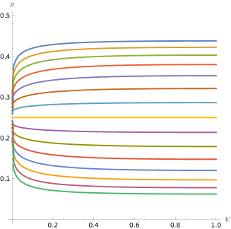
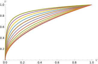
Figure 5: Left: the plot of $\rho$ as a function of $k^{\prime}=\sqrt{1-k^{2}}$ satisfying Equation (9), for various values of $a$ (of the form $2^{j/3}$, with $-7\leq j\leq 7$). Smaller values of $a$ correspond to higher curves. Right: the plot of $b$ as a function of $k^{\prime}$ for several values of $a$ (of the form $2^{j/3}$, $0\leq j\leq 10$). The plot for $a<1$ is the same as for $1/a$.

Remark 10.

• Assuming that the train-track angles are given by $\alpha,\beta,\gamma,\delta$ (independently of $j$) and supposing that $\beta-\alpha=\delta-\gamma=\frac{1}{2}$ imply that Fock’s weights have a period of size $2\times 2$. As a consequence, in the genus 1 case, for general $2\times 2$ periodic weights, on top of the angle parameter $\rho$ and the modular parameter $\tau$, we have one additional parameter $t\in\mathbb{R}/\mathbb{Z}$. This parameter is fixed to the value $+\frac{1}{4}$ in the case of the biased $2\times 2$ periodic weights of [BD23].

• Using the notation of the proof of Proposition 9, for every $\rho\in(0,\frac{1}{2})$, setting $k=0$ (or equivalently $k^{\prime}=1$), amounting to considering the limit $\tau\rightarrow i\mathbb{R}_{+}^{*}$, we obtain $b=1,a=\cot(\pi\rho)\in(0,\infty)$. The genus 1 case degenerates to a genus 0 case, and we recover a parameterization of the 1-periodic weights of [CJY15].

• Returning to the proof of Proposition 9, for every $k^{\prime}\in(0,1)$, choosing $a=1$ corresponds to taking $\rho=\frac{1}{4}$, and according to Equation (12), $b=\sqrt{k^{\prime}}$. We recover a parameterization of the 2-periodic weights of [CY14].

2.4 Space of parameters

The special form of Fock’s weights, see Equation (5), may seem to be restrictive; we explain here that this is not the case. More precisely, we prove that given a dimer model on the Aztec diamond with any positive weight function, it is gauge equivalent to a dimer model with Fock’s weights. Recall from Section 2.1 that the two dimer models then yield the same dimer Boltzmann measure.

Proposition 11.

For any $n\in\mathbb{N}^{*}$, and any choice of positive edge weights $\nu$ on $\mathsf{A}_{n}$, there exists an M-curve $\Sigma$ of genus $g$, a parameter $t\in(\mathbb{R}/\mathbb{Z})^{g}$, and angles ${\bm{\alpha}},{\bm{\beta}},{\bm{\gamma}},{\bm{\delta}}\in A_{0}$ assigned to oriented train-tracks of $\mathsf{A}_{n}$ satisfying ${\bm{\alpha}}<{\bm{\gamma}}<{\bm{\beta}}<{\bm{\delta}}$ on $A_{0}$, such that the dimer models with Fock’s weights and weight function $\nu$ are gauge equivalent.

Proof.

Consider for a moment $\mathsf{A}_{n}$ as a subgraph of the infinite square lattice $\mathbb{Z}^{2}$, and extend the edge weights $\nu$ in a periodic system of weights $\bar{\nu}$ for the whole square lattice. Following [KOS06], we can construct the spectral curve $\mathscr{C}$ associated to the periodic weights $\bar{\nu}$ as the set of zeros of the characteristic polynomial, see [KOS06, Sections 3.1.3, 3.2.3] for definitions. This algebraic curve is a Harnack curve. Moreover, if a vertex is distinguished, there is a natural associated standard divisor, where a standard divisor corresponds to a collection of $g$ points on each oval of $\mathscr{C}$ if $\mathscr{C}$ has genus $g$ [KO06]; this defines the spectral data of the model. The dimer spectral theorem by Kenyon and Okounkov implies that that $\mathscr{C}$ together with its standard divisor (the spectral data) characterize the periodic weights up to gauge transformation. By Remark [BCdT23a, 50.2], which relies on [BCdT23a, Theorem 49] and [GK13, Theorem 7.3], it follows that there is a $t\in(\mathbb{R}/\mathbb{Z})^{g}$ and a periodic assignment of angle parameters to the train-tracks, satisfying the cyclic order condition, such that the corresponding dimer model with periodic Fock’s weights is gauge equivalent to the original one. When restricting back to the subgraph $\mathsf{A}_{n}$, we get weights of the form (5) which are gauge-equivalent to the initial weights $\nu$. ∎

Remark 12.

• In Section 2.3, we prove two explicit realizations of Proposition 11 in the case of Stanley’s weights and of the biased $2\times 2$ periodic weights. In general, making the content of Proposition 11 explicit is not easy because the argument underlying the proof is a general parameterization theorem. The idea to proceed would be to compute the associated characteristic polynomial using the weight function $\nu$, and the associated spectral curve, Newton polygon and amoeba. The genus $g$ is given by the number of holes in the amoeba, and from the tentacles one can recover the angles of the train-tracks. However the parameter $t$ is encoded by a standard divisor on the curve, which is some additional information that needs to be given.

• Note that, generically, holes in the amoeba are in correspondence with integer points in the interior of the Newton polygon; a lower number of holes means that there are isolated singularities on the curve. As a consequence, generically, the genus $g$ of Proposition 11 increases with $n$, the size of the Aztec diamond.

3 Explicit formula for the inverse Kasteleyn matrix

The setting is that of Section 2.2: we consider an M-curve $\Sigma$ of genus $g$, the associated Riemann theta function $\theta$ and prime form $E$, and fix a parameter $t\in(\mathbb{R}/\mathbb{Z})^{g}$; we suppose that oriented train-tracks are assigned angles in $A_{0}$ satisfying condition (4), and consider the associated discrete Abel map $\mathbf{d}$. In this section we state and prove one of the main results of this paper, Theorem 13, consisting of an explicit expression for the inverse of the Kasteleyn matrix with Fock’s weights. Recalling Theorem 5, an immediate consequence of Theorem 13 is an explicit formula for the dimer Boltzmann measure in the very general framework of Fock’s weights. As explained in the introduction, Theorem 13 aims at, in some sense, closing a long history of explicit expressions for the inverse Kasteleyn matrix of the Aztec diamond; refer to Section 1 for historical background.

This section is organised as follows: in Section 3.1, we give some prerequisites, that is, the definition of the forms $g$ in the kernel of the Kasteleyn matrix $\mathsf{K}$ [BCdT23a], and Fay’s identity [Fay73]; then in Section 3.2 we state and prove Theorem 13.

3.1 Prerequisites

Forms in the kernel of $\mathsf{K}$.

We need the following ingredient from [BCdT23a], namely forms in the kernel of the Kasteleyn matrix $\mathsf{K}$, defined as follows. Every edge of $\mathsf{A}^{\diamond}_{n}$ consists of a dual vertex $\mathsf{f}$, and a white or black vertex of $\mathsf{A}_{n}$. For every edge of $\mathsf{A}^{\diamond}_{n}$, and every $u\in\Sigma$, define:

$$g_{\mathsf{f},\mathsf{w}}(u) =g_{\mathsf{w},\mathsf{f}}(u)^{-1}=\frac{\theta(t+u+\mathbf{d}(\mathsf{w}))}{E(\beta,u)}$$ (13)

$$g_{\mathsf{b},\mathsf{f}}(u) =g_{\mathsf{f},\mathsf{b}}(u)^{-1}=\frac{\theta(-t+u-\mathbf{d}(\mathsf{b}))}{E(\alpha,u)},$$ (14)

where $\alpha$, resp. $\beta$, is the angle of the oriented train-track crossing the edge $\mathsf{w}\mathsf{f}$, resp. $\mathsf{b}\mathsf{f}$, see Figure 2. When $\mathsf{x},\mathsf{y}$ are two vertices of $\mathsf{A}^{\diamond}_{n}$, consider a path $\mathsf{x}=\mathsf{x}_{1},\dots,\mathsf{x}_{n}=\mathsf{y}$ of $\mathsf{A}^{\diamond}_{n}$, and set

$$g_{\mathsf{x},\mathsf{y}}(u)=\prod_{j=1}^{n-1}g_{\mathsf{x}_{j},\mathsf{x}_{j+1}}(u).$$

This quantity is well defined, i.e., independent of the choice of path in $\mathsf{A}^{\diamond}_{n}$ from $\mathsf{x}$ to $\mathsf{y}$.

By [BCdT23a, Lemma 33], see also [Foc15] we know that the forms $g$ are in the kernel of $\mathsf{K}$ for vertices that are not on the boundary; written explicitly we have that, for every $u\in\Sigma$, for every vertex $\mathsf{x}$ of $\mathsf{A}^{\diamond}_{n}$, and every white vertex in the bulk of $\mathsf{A}_{n}$,

$$\sum_{\mathsf{b}\sim\mathsf{w}}\mathsf{K}_{\mathsf{w},\mathsf{b}}g_{\mathsf{b},\mathsf{x}}(u)=0.$$ (15)

Fays’ identity.

In the course of the proof of Theorem 13, we will need the following variant of Fay’s identity [Fay73, Proposition 2.10] to expand the product $\mathsf{K}_{\mathsf{w},\mathsf{b}}g_{\mathsf{b},\mathsf{w}}(u)$, see also [BCdT23a, Equation (9)],

$$\mathsf{K}_{\mathsf{w},\mathsf{b}}g_{\mathsf{b},\mathsf{w}}(u) =\frac{E(\alpha,\beta)}{\theta(t+\mathbf{d}(\mathsf{f}))\theta(t+\mathbf{d}(\mathsf{f}^{\prime}))}\frac{\theta(t+u+\mathbf{d}(\mathsf{w}))\theta(-t+u-\mathbf{d}(\mathsf{b}))}{E(\alpha,u)E(\beta,u)}$$

$$=\omega_{\beta-\alpha}+\sum_{\ell=1}^{g}\Bigl{(}\frac{\partial\theta}{\partial z_{\ell}}(t+\mathbf{d}(\mathsf{f}))-\frac{\partial\theta}{\partial z_{\ell}}(t+\mathbf{d}(\mathsf{f}^{\prime}))\Bigr{)}\omega_{j},$$ (16)

where $\omega_{\beta-\alpha}=\mathrm{d}_{u}\log\frac{E(u,\alpha)}{E(u,\beta)}$ is the unique meromorphic 1-form with 0 integral along $A$-cycles, and two simple poles at $\beta$, resp. $\alpha$, with residue $1$, resp. $-1$.

3.2 Explicit formula for the inverse Kasteleyn operator

We consider the Kasteleyn matrix $\mathsf{K}$ with Fock’s weights, see Equation (5). In order to state our explicit formula for the inverse matrix, we first define contours of integration. By assumption, the angles assigned to oriented train-tracks satisfy the cyclic condition (4): ${\bm{\alpha}}<{\bm{\gamma}}<{\bm{\beta}}<{\bm{\delta}}.$ This implies that the real component $A_{0}$ of $\Sigma$ can naturally be split into four disjoint connected subsets containing all of the angles of one type and none of the other types. We let $\mathscr{C}_{1}$ be a trivial contour on $\Sigma$, oriented counterclockwise, containing in its interior all of the angles ${\bm{\gamma}}=(\gamma_{j})_{j=1}^{n}$ and none of the angles ${\bm{\alpha}},{\bm{\beta}},{\bm{\delta}}$.

Similarly $\mathscr{C}_{2}$ is a trivial contour on $\Sigma$, oriented counterclockwise, containing in its interior all of the angles ${\bm{\alpha}}=(\alpha_{j})_{j=1}^{n}$ and none of the others.

Theorem 13.

For every pair $(\mathsf{b},\mathsf{w})$ of black and white vertices of $\mathsf{A}_{n}$, the coefficient $(\mathsf{b},\mathsf{w})$ of the inverse Kasteleyn matrix is explicitly given by

$$\mathsf{K}^{-1}_{\mathsf{b},\mathsf{w}}=\frac{1}{(2\pi i)^{2}}\frac{1}{\theta(p)}\int_{\mathscr{C}_{2}}\int_{\mathscr{C}_{1}}\frac{\theta(p+(v-u))}{E(u,v)}g_{\mathsf{b},0}(u)g_{0,\mathsf{w}}(v)\prod_{j=1}^{n}\frac{E(\beta_{j},u)}{E(\delta_{j},u)}\frac{E(\delta_{j},v)}{E(\beta_{j},v)}+\\ -\mathbb{I}_{\{\mathsf{b}\text{ right of }\mathsf{w}\}}\frac{1}{2\pi i}\int_{\mathscr{C}_{2}}g_{\mathsf{b},\mathsf{w}}(v),$$ (17)

where $\mathscr{C}_{1}$, resp. $\mathscr{C}_{2}$, is the closed contour defined above used to integrate over $u$, resp. $v$, and $p=\sum\limits_{j=1}^{n}(\delta_{j}-\beta_{j})-t-\mathbf{d}(0)$.

Before turning to the proof, let us make a few remarks.

Remark 14.

• The integrand, seen as function of $u$, resp. $v$, is a meromorphic $1$-form. Indeed, looking at terms involving prime forms and recalling that the prime form is a $(-\frac{1}{2},-\frac{1}{2})$ form, we have that the integrand is a $1$-form. Moreover, an explicit computation shows that this $1$-form has no period when $u$, resp. $v$, is translated by a horizontal/vertical period of the lattice $\Lambda$, implying that it is meromorphic.

• In the double integral of (17) the factor $g_{\mathsf{b},0}(u)\prod_{j}\frac{E(\beta_{j},u)}{E(\delta_{j},u)}$ has poles at every $\gamma_{j}$ on the left of $\mathsf{b}$ and every $\delta_{j}$ on the right of $\mathsf{b}$, and zeros at every $\alpha_{j}$ below $\mathsf{b}$ and every $\beta_{j}$ above $\mathsf{b}$; similarly for $g_{0,\mathsf{w}}(v)\prod_{j}\frac{E(\delta_{j},v)}{E(\beta_{j},v)}$, where the role of poles and zeros are exchanged. As a consequence, we can deform the contours of integration without changing the value of the integral if we do not cross poles. For example, one could move $\mathscr{C}_{1}$ into another contour $\mathscr{C}_{1}^{\prime}$ to also include the $\beta_{j}$’s in its interior, and replace $\mathscr{C}_{2}$ by $\mathscr{C}_{2}^{\prime}$ depicted on Figure 6, which is now oriented clockwise, and contains on its right the points from ${\bm{\gamma}}$ and ${\bm{\beta}}$ (but not those from ${\bm{\alpha}}$). The relative position of $\mathscr{C}_{1}$ and $\mathscr{C}_{2}$ is important because of the presence of $E(u,v)$ in the denominator of the integrand. The contribution of the residue at $u=v$ is exactly given by the single contour integral in front of the indicator function. We can therefore absorb this second term inside the double contour integral by indicating that when $\mathsf{b}$ is on the right of $\mathsf{w}$, we require that $\mathscr{C}_{1}^{\prime}$ is inside $\mathscr{C}_{2}^{\prime}$ (instead of outside).

  

  

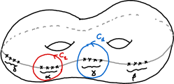
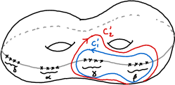
  Figure 6: A possible deformation of integration contours for Formula (17).

• The point $0=(0,0)$ seems to play a particular role in the formula: in the definition of $p$ and in the arguments of the functions $g$. This is actually not the case, one could express $p$ and the product $g$ times the terms involving the prim forms using another reference point and the geometry of the Aztec diamond.

• Examples of Theorem 13 in specific cases are given after the proof.

Proof.

Although our setting is much more general than the paper [CJY15], our inspiration for this proof and choice of notation is inspired by the latter. Consider two white vertices $\mathsf{w},\mathsf{w}^{\prime}$; the proof consists in showing that

$$(\mathsf{K}\mathsf{K}^{-1})_{\mathsf{w},\mathsf{w}^{\prime}}=\sum_{\mathsf{b}\sim\mathsf{w}}\mathsf{K}_{\mathsf{w},\mathsf{b}}\mathsf{K}^{-1}_{\mathsf{b},\mathsf{w}^{\prime}}=\mathbb{I}_{\{\mathsf{w}=\mathsf{w}^{\prime}\}}.$$

Let us denote by $f^{1}$, resp. $f^{2}$, the first, resp. second term of Equation (17):

$$f^{1}_{\mathsf{b},\mathsf{w}} =\frac{1}{(2\pi i)^{2}}\frac{1}{\theta(p)}\int_{\mathscr{C}_{2}}\int_{\mathscr{C}_{1}}\frac{\theta(p+(v-u))}{E(u,v)}g_{\mathsf{b},0}(u)g_{0,\mathsf{w}}(v)\prod_{j=1}^{n}\frac{E(\beta_{j},u)}{E(\delta_{j},u)}\frac{E(\delta_{j},v)}{E(\beta_{j},v)}$$ (18)

$$f^{2}_{\mathsf{b},\mathsf{w}} =\mathbb{I}_{\{\mathsf{b}\text{ right of }\mathsf{w}\}}\frac{1}{2\pi i}\int_{\mathscr{C}_{2}}g_{\mathsf{b},\mathsf{w}}(v).$$ (19)

The proof requires the following 5 steps. If $\mathsf{w},\mathsf{w}^{\prime}$ are such that

1. $\mathsf{w}_{x}\neq 2n$ and $\mathsf{w}_{x}\neq\mathsf{w}_{x}^{\prime}$, or $\mathsf{w}_{x}=\mathsf{w}_{x}^{\prime}=2n$, then $(\mathsf{K}f^{2})_{\mathsf{w},\mathsf{w}^{\prime}}=0$.

2. $\mathsf{w}_{x}\neq 2n$ and $\mathsf{w}_{x}=\mathsf{w}_{x}^{\prime}$, then $(\mathsf{K}f^{2})_{\mathsf{w},\mathsf{w}^{\prime}}=-\mathbb{I}_{\{\mathsf{w}=\mathsf{w}^{\prime}\}}.$

3. $\mathsf{w}_{x}\neq 2n$, then $(\mathsf{K}f^{1})_{\mathsf{w},\mathsf{w}^{\prime}}=0$.

4. $\mathsf{w}_{x}=2n$ and $\mathsf{w}_{x}\neq\mathsf{w}_{x}^{\prime}$, then $(\mathsf{K}f^{1})_{\mathsf{w},\mathsf{w}^{\prime}}=(\mathsf{K}f^{2})_{\mathsf{w},\mathsf{w}^{\prime}}$.

5. $\mathsf{w}_{x}=2n$ and $\mathsf{w}_{x}=\mathsf{w}_{x}^{\prime}$, then $(\mathsf{K}f^{1})_{\mathsf{w},\mathsf{w}^{\prime}}=\mathbb{I}_{\{\mathsf{w}=\mathsf{w}^{\prime}\}}.$

Before proving each of the steps, let us show that they indeed allow to end the proof. If $\mathsf{w}$ is such that:

• $\mathsf{w}_{x}\in\{0,2,\dots,2n-2\}$, and $\mathsf{w}_{x}\neq\mathsf{w}_{x}^{\prime}$, then by Point 1. we have $(\mathsf{K}f^{2})_{\mathsf{w},\mathsf{w}^{\prime}}=0$, and by Point 3. $(\mathsf{K}f^{1})_{\mathsf{w},\mathsf{w}^{\prime}}=0$, implying that $(\mathsf{K}\mathsf{K}^{-1})_{\mathsf{w},\mathsf{w}^{\prime}}=0$.

• $\mathsf{w}_{x}\in\{0,2,\dots,2n-2\}$, and $\mathsf{w}_{x}=\mathsf{w}^{\prime}_{x}$, then by Point 2. we have $(\mathsf{K}f^{2})_{\mathsf{w},\mathsf{w}^{\prime}}=-\mathbb{I}_{\{\mathsf{w}=\mathsf{w}^{\prime}\}}$, and by Point 3. $(\mathsf{K}f^{1})_{\mathsf{w},\mathsf{w}^{\prime}}=0$, implying that $(\mathsf{K}\mathsf{K}^{-1})_{\mathsf{w},\mathsf{w}^{\prime}}=\mathbb{I}_{\{\mathsf{w}=\mathsf{w}^{\prime}\}}$.

• $\mathsf{w}_{x}=2n$ and $\mathsf{w}_{x}\neq\mathsf{w}_{x}^{\prime}$, then by Point 4, $(\mathsf{K}f^{1})_{\mathsf{w},\mathsf{w}^{\prime}}=(\mathsf{K}f^{2})_{\mathsf{w},\mathsf{w}^{\prime}}$, implying that $(\mathsf{K}\mathsf{K}^{-1})_{\mathsf{w},\mathsf{w}^{\prime}}=0$.

• $\mathsf{w}_{x}=2n$ and $\mathsf{w}_{x}=\mathsf{w}_{x}^{\prime}$ then by Point 1. we have $(\mathsf{K}f^{2})_{\mathsf{w},\mathsf{w}^{\prime}}=0$, and by Point 5. $(\mathsf{K}f^{1})_{\mathsf{w},\mathsf{w}^{\prime}}=\mathbb{I}_{\{\mathsf{w}=\mathsf{w}^{\prime}\}}$, implying that $(\mathsf{K}\mathsf{K}^{-1})_{\mathsf{w},\mathsf{w}^{\prime}}=\mathbb{I}_{\{\mathsf{w}=\mathsf{w}^{\prime}\}}$.

We now turn to the proof of Points 1. to 5.

1. When $\mathsf{w}_{x}^{\prime}>\mathsf{w}_{x}$, all $\mathsf{b}$-neighbors of $\mathsf{w}$ are on the left of $\mathsf{w}^{\prime}$, so that all terms of type $f_{2}$ are equal to 0 and $(\mathsf{K}f^{2})_{\mathsf{w},\mathsf{w}^{\prime}}$ is trivially equal to 0 (note that there are four neighbors if $\mathsf{w}_{x}\neq 0$ and two neighbors if $\mathsf{w}_{x}=0$). If $\mathsf{w}_{x}=\mathsf{w}_{x}^{\prime}=2n$, the same holds since then the two $\mathsf{b}$-neighbors of $\mathsf{w}$ are on the left of $\mathsf{w}^{\prime}$ and there are no right neighbors. When $\mathsf{w}_{x}^{\prime}<\mathsf{w}_{x}$ and $\mathsf{w}_{x}\neq 2n$, the four $\mathsf{b}$-neighbors of $\mathsf{w}$ are now on the right, and there are four contributions of type $f_{2}$. We have

$$(\mathsf{K}f^{2})_{\mathsf{w},\mathsf{w}^{\prime}} =\frac{1}{2\pi i}\sum_{\mathsf{b}\sim\mathsf{w}}\int_{\mathscr{C}_{2}}\mathsf{K}_{\mathsf{w},\mathsf{b}}\,g_{\mathsf{b},\mathsf{w}^{\prime}}.$$

Since the contour $\mathscr{C}_{2}$ in independent of $\mathsf{b},\mathsf{w}^{\prime}$, the sum can be moved inside the integral, and we have that $(\mathsf{K}f^{2})_{\mathsf{w},\mathsf{w}^{\prime}}$ is equal to $0$ by Equation (15).

2. Suppose that $\mathsf{w}_{x}=\mathsf{w}_{x}^{\prime}$ and $\mathsf{w}_{x}\neq 2n$. Let $\mathsf{b}_{1},\mathsf{b}_{2}$ be the two neighbors of $\mathsf{w}$ on the right, from bottom to top, and $\mathsf{f}_{1},\mathsf{f}_{2},\mathsf{f}_{3}$ be the dual vertices as in Figure 7.

\begin{overpic}[width=170.71652pt]{fig_proof_Kinv_1.pdf} \put(15.0,28.0){\scriptsize$\alpha$} \put(19.0,33.0){\scriptsize$\gamma$} \put(15.0,42.0){\scriptsize$\beta$} \put(6.0,32.0){\scriptsize$\delta$} \put(9.0,36.0){\scriptsize$\mathsf{w}$} \put(8.0,80.0){\scriptsize$\mathsf{w}^{\prime}$} \put(27.0,25.0){\scriptsize$\mathsf{b}_{1}$} \put(27.0,48.0){\scriptsize$\mathsf{b}_{2}$} \put(12.0,21.0){\scriptsize$\mathsf{f}_{1}$} \put(27.0,36.0){\scriptsize$\mathsf{f}_{2}$} \put(10.0,49.0){\scriptsize$\mathsf{f}_{3}$} \put(87.0,50.0){\scriptsize$\alpha$} \put(91.0,57.0){\scriptsize$\gamma$} \put(87.0,64.0){\scriptsize$\beta$} \put(77.0,56.0){\scriptsize$\delta$} \put(80.0,60.0){\scriptsize$\mathsf{w}$} \put(80.0,15.0){\scriptsize$\mathsf{w}^{\prime}$} \end{overpic}

Figure 7: Zeros and poles of $g_{\mathsf{w},\mathsf{w}^{\prime}}(v)$ when $\mathsf{w}_{x}=\mathsf{w}_{x}^{\prime}$, $\mathsf{w}_{x}\neq 2n$. Left: $\mathsf{w}^{\prime}$ is above $\mathsf{w}$. Right: $\mathsf{w}^{\prime}$ is below $\mathsf{w}$. Angles corresponding to zeros, resp. poles, are pictured in green, resp. magenta.

Using that the contour of integration $\mathscr{C}_{2}$ is independent of $\mathsf{b}_{1},\mathsf{b}_{2},\mathsf{w}^{\prime}$, and using the product structure of the meromorphic form $g$, we obtain

$$(\mathsf{K}f^{2})_{\mathsf{w},\mathsf{w}^{\prime}}=\frac{1}{2\pi i}\int_{\mathscr{C}_{2}}\Bigl{[}\sum_{i=1}^{2}\mathsf{K}_{\mathsf{w},\mathsf{b}_{i}}g_{\mathsf{b}_{i},\mathsf{w}}(v)\Bigr{]}g_{\mathsf{w},\mathsf{w}^{\prime}}(v).$$

To simplify notation, we write the four angles around $\mathsf{w}$ as $\alpha,\gamma,\beta,\delta$ going cclw starting from the bottom (omitting indices). From Fay’s identity (16) we have

$$\sum_{i=1}^{2}\mathsf{K}_{\mathsf{w},\mathsf{b}_{i}}g_{\mathsf{b}_{i},\mathsf{w}}(v) =\omega_{\gamma-\alpha}+\sum_{\ell=1}^{g}\Bigl{(}\frac{\partial\log\theta}{\partial z_{\ell}}(t+\mathbf{d}(\mathsf{f}_{3}))-\frac{\partial\log\theta}{\partial z_{\ell}}(t+\mathbf{d}(\mathsf{f}_{2}))\Bigr{)}\omega_{\ell}$$

$$\quad\quad\quad\quad+\omega_{\beta-\gamma}+\sum_{\ell=1}^{g}\Bigl{(}\frac{\partial\log\theta}{\partial z_{\ell}}(t+\mathbf{d}(\mathsf{f}_{2}))-\frac{\partial\log\theta}{\partial z_{\ell}}(t+\mathbf{d}(\mathsf{f}_{1}))\Bigr{)}\omega_{\ell}$$

$$=\omega_{\beta-\alpha}+\sum_{\ell=1}^{g}\Bigl{(}\frac{\partial\log\theta}{\partial z_{\ell}}(t+\mathbf{d}(\mathsf{f}_{3}))-\frac{\partial\log\theta}{\partial z_{\ell}}(t+\mathbf{d}(\mathsf{f}_{1}))\Bigr{)}\omega_{\ell}.$$ (20)

As a consequence,

$$(\mathsf{K}f^{2})_{\mathsf{w},\mathsf{w}^{\prime}} =\frac{1}{2\pi i}\Bigl{(}\int_{\mathscr{C}_{2}}g_{\mathsf{w},\mathsf{w}^{\prime}}(v)\,\omega_{\beta-\alpha}+\sum_{\ell=1}^{g}\Bigl{(}\frac{\partial\log\theta}{\partial z_{\ell}}(t+\mathbf{d}(\mathsf{f}_{3}))-\frac{\partial\log\theta}{\partial z_{\ell}}(t+\mathbf{d}(\mathsf{f}_{1}))\Bigr{)}\int_{\mathscr{C}_{2}}g_{\mathsf{w},\mathsf{w}^{\prime}}(v)\,\omega_{\ell}\Bigr{)}.$$

Returning to the definition of the form $g$, we know that the zeros, resp. poles, of $g_{\mathsf{w},\mathsf{w}^{\prime}}(v)$ in $\mathscr{C}_{2}$ are the angles between $\mathsf{w}$ and $\mathsf{w}^{\prime}$ of type

• $(\beta_{j})$ (including $\beta$) , resp. $(\alpha_{j})$ (excluding $\alpha$), when $\mathsf{w}^{\prime}$ is above $\mathsf{w}$, see Figure 7 (left),

• $(\alpha_{j})$ (including $\alpha)$, resp. $(\beta_{j})$ (excluding $\beta$), when $\mathsf{w}^{\prime}$ is below $\mathsf{w}$, see Figure 7 (right).

Let us first consider the term $\frac{1}{2\pi i}\int_{\mathscr{C}_{2}}g_{\mathsf{w},\mathsf{w}^{\prime}}(v)\,\omega_{\beta-\alpha}\,$.

• when $\mathsf{w}^{\prime}$ is above $\mathsf{w}$, the pole at $\beta$ of $\omega_{\beta-\alpha}$ is cancelled by the zero at $\beta$ of $g_{\mathsf{w},\mathsf{w}^{\prime}}(v)$, and the integrand $\omega_{\beta-\alpha}\,g_{\mathsf{w},\mathsf{w}^{\prime}}(v)$ has as poles a subset of $\{\alpha_{1},\dots,\alpha_{n}\}$. Since the contour $\mathscr{C}_{2}$ contains all the angles $\{\alpha_{1},\dots,\alpha_{n}\}$, we obtain 0.

• when $\mathsf{w}^{\prime}$ is below $\mathsf{w}$, the pole at $\alpha$ of $\omega_{\beta-\alpha}$ is cancelled by the zero at $\alpha$ of $g_{\mathsf{w},\mathsf{w}^{\prime}}(v)$, and the integrand has as poles a subset of $\{\beta_{1},\dots,\beta_{n}\}$. Since the contour $\mathscr{C}_{2}$ contains none of these poles, we also obtain 0.

• when $\mathsf{w}=\mathsf{w}^{\prime}$, then $g_{\mathsf{w},\mathsf{w}}(v)=1$, and the contour $\mathscr{C}_{2}$ contains the pole $\alpha$ of $\omega_{\beta-\alpha}$, which yields that $\frac{1}{2\pi i}\int_{\mathscr{C}_{2}}\omega_{\beta-\alpha}=-1$.

Let us now consider the term $\int_{\mathscr{C}_{2}}g_{\mathsf{w},\mathsf{w}^{\prime}}(v)\,\omega_{\ell}$. The contour $\mathscr{C}_{2}$ either contains all poles of $g_{\mathsf{w},\mathsf{w}^{\prime}}$ (when $\mathsf{w}^{\prime}$ is above $\mathsf{w}$) or none of them (if $\mathsf{w}^{\prime}$ is below or equal to $\mathsf{w}$), and the integral of the form $\omega_{\ell}$ around any trivial closed contour is 0, so that the second term is always equal to 0. Summarizing, we have proved Point 2.

$$(\mathsf{K}f^{2})_{\mathsf{w},\mathsf{w}^{\prime}}=\frac{1}{2\pi i}\int_{\mathscr{C}_{2}}\Bigl{[}\sum_{i=1}^{2}\mathsf{K}_{\mathsf{w},\mathsf{b}_{i}}g_{\mathsf{b}_{i},\mathsf{w}^{\prime}}(v)\Bigr{]}=-\mathbb{I}_{\{\mathsf{w}=\mathsf{w}^{\prime}\}}.$$ (21)

3. Using that the contours of integration $\mathscr{C}_{1},\mathscr{C}_{2}$ are independent of $\mathsf{b},\mathsf{w}^{\prime}$, we have, for every pair of white vertices $(\mathsf{w},\mathsf{w}^{\prime})$,

$$(\mathsf{K}f^{1})_{\mathsf{w},\mathsf{w}^{\prime}}=$$

$$=\frac{1}{(2\pi i)^{2}}\frac{1}{\theta(p)}\sum_{\mathsf{b}\sim\mathsf{w}}\mathsf{K}_{\mathsf{w},\mathsf{b}}\int_{\mathscr{C}_{2}}\int_{\mathscr{C}_{1}}\frac{\theta(p+(v-u))}{E(u,v)}g_{\mathsf{b},0}(u)g_{0,\mathsf{w}^{\prime}}(v)\prod_{j=1}^{n}\frac{E(\beta_{j},u)}{E(\delta_{j},u)}\frac{E(\delta_{j},v)}{E(\beta_{j},v)}$$

$$=\frac{1}{(2\pi i)^{2}}\frac{1}{\theta(p)}\int_{\mathscr{C}_{2}}g_{0,\mathsf{w}^{\prime}}(v)\prod_{j=1}^{n}\frac{E(\delta_{j},v)}{E(\beta_{j},v)}\cdot$$

$$\hskip 71.13188pt\cdot\int_{\mathscr{C}_{1}}\frac{\theta(p+(v-u))}{E(u,v)}\prod_{j=1}^{n}\frac{E(\beta_{j},u)}{E(\delta_{j},u)}\Bigl{[}\sum_{\mathsf{b}\sim\mathsf{w}}\mathsf{K}_{\mathsf{w},\mathsf{b}}g_{\mathsf{b},0}(u)\Bigr{]}.$$ (22)

As a consequence, when $\mathsf{w}_{x}\notin\{0,2n\}$, this is equal to 0 by Equation (15). When $\mathsf{w}_{x}=0$, one can insert a column of black vertices on the left, and an angle $\delta_{0}$ (in the sector containing $\{\delta_{1},\dots,\delta_{n}\}$). In this way, the white vertex $\mathsf{w}$ has its four $\mathsf{b}$-neighbors: $\mathsf{b}_{1},\mathsf{b}_{2}$ present in the original Aztec diamond, and $\mathsf{b}_{3},\mathsf{b}_{4}$ the two additional ones. Note that defining $f^{1}_{\mathsf{b}_{i},\mathsf{w}}$ ($i\in\{3,4\}$) using Formula (18) gives 0 in this case. Indeed, $g_{\mathsf{b}_{i},0}(u)$ has as poles $\delta_{0}$ and a subset of the angles $(\beta_{j})$, implying that the contour $\mathscr{C}_{1}$ (which contains all of the angles $\{\gamma_{1},\dots,\gamma_{n}\}$) contains no pole of the integrand $g_{\mathsf{b}_{i},0}(u)\frac{\theta(p+(v-u))}{E(u,v)}\prod_{j=1}^{n}\frac{E(u,\beta_{j})}{E(u,\delta_{j})}$, yielding 0. The proof can then be concluded using Equation (15) again.

4. Suppose $\mathsf{w}_{x}=2n$, and let $\mathsf{b}_{3},\mathsf{b}_{4}$ be the two neighbors of $\mathsf{w}$ on the left, from bottom to top, and $\mathsf{f}_{1},\mathsf{f}_{3},\mathsf{f}_{4}$ be the dual vertices as in Figure 8.

\begin{overpic}[width=170.71652pt]{fig_proof_Kinv_2.pdf} \put(98.0,43.0){\scriptsize$\alpha$} \put(98.0,60.0){\scriptsize$\beta$} \put(82.0,51.0){\scriptsize$\delta_{n}$} \put(100.0,50.0){\scriptsize$\mathsf{w}$} \par\put(73.0,35.0){\scriptsize$\mathsf{b}_{3}$} \put(73.0,63.0){\scriptsize$\mathsf{b}_{4}$} \put(95.0,29.0){\scriptsize$\mathsf{f}_{1}$} \put(74.0,50.0){\scriptsize$\mathsf{f}_{4}$} \put(95.0,67.0){\scriptsize$\mathsf{f}_{3}$} \par\put(-5.0,12.0){\scriptsize$\alpha_{1}$} \put(8.0,-3.0){\scriptsize$\gamma_{1}$} \put(-5.0,28.0){\scriptsize$\beta_{1}$} \put(26.0,-4.0){\scriptsize$\delta_{1}$} \put(0.0,0.0){\scriptsize$0$} \end{overpic}

Figure 8: Zeros and poles of $g_{\mathsf{w},\mathsf{w}^{\prime}}(v)$ when $\mathsf{w}_{x}=\mathsf{w}_{x}^{\prime}$, $\mathsf{w}_{x}\neq 2n$. Left: $\mathsf{w}^{\prime}$ is above $\mathsf{w}$. Right: $\mathsf{w}^{\prime}$ is below $\mathsf{w}$. Angles corresponding to zeros, resp. poles, are pictured in green, resp. magenta.

To simplify notation, let us denote by $\alpha,\delta_{n},\beta$ the angles around $\mathsf{w}$ in clockwise order (omitting the indices for $\alpha,\beta$). Writing $(\mathsf{K}f^{1})_{\mathsf{w},\mathsf{w}^{\prime}}$ as in Equation (22), we first consider the part containing the integral over $\mathscr{C}_{1}$.

$$\int_{\mathscr{C}_{1}}\frac{\theta(p+(v-u))}{E(u,v)}\Bigl{[}\sum_{i=3}^{4}\mathsf{K}_{\mathsf{w},\mathsf{b}_{i}}g_{\mathsf{b}_{i},\mathsf{w}}(u)\Bigr{]}g_{\mathsf{w},0}(u)\prod_{j=1}^{n}\frac{E(\beta_{j},u)}{E(\delta_{j},u)}.$$ (23)

Similarly to Equation (3.2), using Fay’s identity (16) gives

$$\sum_{i=3}^{4}\mathsf{K}_{\mathsf{w},\mathsf{b}_{i}}g_{\mathsf{b}_{i},\mathsf{w}}(v) =\omega_{\alpha-\beta}+\sum_{\ell=1}^{g}\Bigl{(}\frac{\partial\log\theta}{\partial z_{\ell}}(t+\mathbf{d}(\mathsf{f}_{1}))-\frac{\partial\log\theta}{\partial z_{\ell}}(t+\mathbf{d}(\mathsf{f}_{3}))\Bigr{)}\omega_{\ell}.$$

Note that by definition of $g$, all poles of $g_{\mathsf{b}_{i},0}(u)$ are on $A_{0}$. Now, the term $g_{\mathsf{w},0}(u)$ contains

• as poles on $A_{0}$: all the angles $\gamma_{1},\dots,\gamma_{n}$ and the angles of type $(\beta_{j})$ from $\mathsf{w}$ to the bottom boundary (and in particular not the angle $\beta$),

• as zeros on $A_{0}$: the angles $\delta_{1},\dots,\delta_{n}$ and the angles of type $(\alpha_{j})$ from $\mathsf{w}$ to the bottom boundary (and in particular the angle $\alpha$),

so the product $g_{\mathsf{w},0}(u)\,\omega_{\alpha-\beta}$ contains as poles on $A_{0}$: a subset of the angles of type $(\beta_{j})$, no angle of type $(\alpha_{j})$ (since the pole $\alpha$ of $\omega_{\alpha-\beta}$ is cancelled by the zero $\alpha$ of $g_{\mathsf{w},0}(u)$), all the angles $\gamma_{1},\dots,\gamma_{n}$; note that the set of poles of $g_{\mathsf{w},0}(u)\omega_{\ell}$ has the same property. As a consequence when each of theses terms gets multiplied by $\frac{\theta(p+(v-u))}{E(u,v)}\prod_{j=1}^{n}\frac{E(\beta_{j},u)}{E(\delta_{j},u)}$; all the poles involving angles $(\beta_{j})$ are cancelled, and moreover, the new poles involving $\delta_{1},\dots,\delta_{n}$ are cancelled by the same zeros in $g_{\mathsf{w},0}(u)$. Summarizing, in the integrand

$$\frac{\theta(p+(v-u))}{E(u,v)}\Bigl{[}\sum_{i=3}^{4}\mathsf{K}_{\mathsf{w},\mathsf{b}_{i}}g_{\mathsf{b}_{i},\mathsf{w}}(u)\Bigr{]}g_{\mathsf{w},0}(u)\prod_{j=1}^{n}\frac{E(\beta_{j},u)}{E(\delta_{j},u)},$$

there remains as poles on $\Sigma$: all the angles $\gamma_{1},\dots,\gamma_{n}$ and the pole at $u=v$. By definition, the contour of integration $\mathscr{C}_{1}$ contains all of the angles $\{\gamma_{1},\dots,\gamma_{n}\}$, and the pole $v$ (which lives on $\mathscr{C}_{2}$) is outside of $\mathscr{C}_{1}$. Since we are integrating a meromorphic form on a compact surface (implying that the sum of the residues is equal to 0), the integral (23) is equal to $-2\pi i$ times the residue at $u=v$. Noting that the residue at $u=v$ of $\frac{1}{E(u,v)}$ is equal to $-1$, we obtain:

$$\frac{1}{2\pi i}\frac{1}{\theta(p)}\int_{\mathscr{C}_{1}}\frac{\theta(p+(v-u))}{E(u,v)}\Bigl{[}\sum_{i=3}^{4}\mathsf{K}_{\mathsf{w},\mathsf{b}_{i}}g_{\mathsf{b}_{i},\mathsf{w}}(u)\Bigr{]}g_{\mathsf{w},0}(u)\prod_{j=1}^{n}\frac{E(\beta_{j},u)}{E(\delta_{j},u)}\\ =\Bigl{[}\sum_{i=3}^{4}\mathsf{K}_{\mathsf{w},\mathsf{b}_{i}}g_{\mathsf{b}_{i},\mathsf{w}}(v)\Bigr{]}g_{\mathsf{w},0}(v)\prod_{j=1}^{n}\frac{E(\beta_{j},v)}{E(\delta_{j},v)}=\sum_{i=3}^{4}\mathsf{K}_{\mathsf{w},\mathsf{b}_{i}}g_{\mathsf{b}_{i},0}(v)\prod_{j=1}^{n}\frac{E(\beta_{j},v)}{E(\delta_{j},v)}.$$

Plugging this back into (22) yields,

$$(\mathsf{K}f^{1})_{\mathsf{w},\mathsf{w}^{\prime}} =\frac{1}{2\pi i}\int_{\mathscr{C}_{2}}g_{0,\mathsf{w}^{\prime}}(v)\prod_{j=1}^{n}\frac{E(\delta_{j},v)}{E(\beta_{j},v)}\sum_{i=3}^{4}\mathsf{K}_{\mathsf{w},\mathsf{b}_{i}}g_{\mathsf{b}_{i},0}(v)\prod_{j=1}^{n}\frac{E(\beta_{j},v)}{E(\delta_{j},v)}$$

$$=\frac{1}{2\pi i}\int_{\mathscr{C}_{2}}\sum_{i=3}^{4}\mathsf{K}_{\mathsf{w},\mathsf{b}_{i}}g_{\mathsf{b}_{i},\mathsf{w}^{\prime}}(v).$$ (24)

Now, suppose moreover that $\mathsf{w}_{x}\neq\mathsf{w}_{x}^{\prime}$, then the two $\mathsf{b}$-neighbors of $\mathsf{w}$ are on the right of $\mathsf{w}$, and we have that

$$(\mathsf{K}f^{1})_{\mathsf{w},\mathsf{w}^{\prime}}=(\mathsf{K}f^{2})_{\mathsf{w},\mathsf{w}^{\prime}}.$$

5. Suppose that $\mathsf{w}_{x}=2n$ and $\mathsf{w}_{x}=\mathsf{w}_{x}^{\prime}$. Then, by Equation (24), we have

$$(\mathsf{K}f^{1})_{\mathsf{w},\mathsf{w}^{\prime}}=\frac{1}{2\pi i}\int_{\mathscr{C}_{2}}\sum_{i=3}^{4}\mathsf{K}_{\mathsf{w},\mathsf{b}_{i}}g_{\mathsf{b}_{i},\mathsf{w}^{\prime}}(v).$$

Using the argument of Point 2. with black vertices on the left rather than on the right allows us to conclude that $(\mathsf{K}f^{1})_{\mathsf{w},\mathsf{w}^{\prime}}=\mathbb{I}_{\{\mathsf{w}=\mathsf{w}^{\prime}\}}$. ∎

Example 15.

As an example of application, let us make explicit the case where angles in each family are constant, i.e., suppose that ${\bm{\alpha}}\equiv\alpha,{\bm{\beta}}=\beta,{\bm{\gamma}}=\gamma,{\bm{\delta}}=\delta$, for some angles $\alpha,\beta,\gamma,\delta\in A_{0}$ satisfying the cyclic order $\alpha<\gamma<\beta<\delta$. Recalling the coordinate notation $\mathsf{w}=(\mathsf{w}_{x},\mathsf{w}_{y})$, $\mathsf{b}=(\mathsf{b}_{x},\mathsf{b}_{y})$, we obtain

$$\mathsf{K}^{-1}_{\mathsf{b},\mathsf{w}}=\frac{1}{(2\pi i)^{2}}\frac{1}{\theta(p)}\int_{\mathscr{C}_{2}}\int_{\mathscr{C}_{1}}\frac{\theta(p+(v-u))}{E(u,v)}\cdot\\ \quad\cdot\ \theta(-t+u-\mathbf{d}(\mathsf{b}))\frac{E(\alpha,u)^{\frac{\mathsf{b}_{y}}{2}}E(\beta,u)^{n-\frac{\mathsf{b}_{y}}{2}}}{E(\gamma,u)^{\frac{\mathsf{b}_{x}+1}{2}}E(\delta,u)^{n-{\frac{\mathsf{b}_{x}-1}{2}}}}\theta(t+v+\mathbf{d}(\mathsf{w}))\frac{E(\gamma,v)^{\frac{\mathsf{w}_{x}}{2}}E(\delta,v)^{n-\frac{\mathsf{w}_{x}}{2}}}{E(\beta,v)^{n-\frac{\mathsf{w}_{y}-1}{2}}E(\alpha,v)^{\frac{\mathsf{w}_{y}+1}{2}}}\\ \quad-\mathbb{I}_{\{\mathsf{b}\text{ right of }\mathsf{w}\}}\frac{1}{2\pi i}\int_{\mathscr{C}_{2}}\theta(-t+v-\mathbf{d}(\mathsf{b}))\theta(t+v+\mathbf{d}(\mathsf{w}))\frac{E(\alpha,v)^{\frac{\mathsf{b}_{y}-\mathsf{w}_{y}-1}{2}}}{E(\beta,v)^{\frac{\mathsf{b}_{y}-\mathsf{w}_{y}+1}{2}}}\frac{E(\delta,v)^{\frac{\mathsf{b}_{x}-\mathsf{w}_{x}-1}{2}}}{E(\gamma,v)^{\frac{\mathsf{b}_{x}-\mathsf{w}_{x}+1}{2}}},$$ (25)

where $p=n(\delta-\beta)-t-\mathbf{d}(0)$, and

$$\mathbf{d}(\mathsf{b})=\frac{\mathsf{b}_{y}}{2}(\beta-\alpha)+\frac{\mathsf{b}_{x}+1}{2}\gamma-\frac{\mathsf{b}_{x}-1}{2}\delta,\quad\mathbf{d}(\mathsf{w})=\frac{\mathsf{w}_{x}}{2}(\gamma-\delta)-\frac{\mathsf{w}_{y}+1}{2}\alpha+\frac{\mathsf{w}_{y}-1}{2}\beta.$$

In particular, if $\mathsf{b}$ is the south-west neighbor of $\mathsf{w}$, meaning that $(\mathsf{w}_{x},\mathsf{w}_{y})=(2i,2j+1)$ and $(\mathsf{b}_{x},\mathsf{b}_{y})=(2i-1,2j)$ for some $1\leq i\leq n$ and $0\leq j\leq n-1$, Formula (25) reduces further to

$$\mathsf{K}^{-1}_{\mathsf{b},\mathsf{w}}=\frac{1}{(2\pi i)^{2}}\frac{1}{\theta(p)}\int_{\mathscr{C}_{2}}\int_{\mathscr{C}_{1}}\frac{\theta(p+(v-u))}{E(u,v)}\cdot\theta(-t+u-\mathbf{d}(\mathsf{b}))\theta(t+v+\mathbf{d}(\mathsf{w}))\\ \cdot\frac{E(\alpha,u)^{j}E(\beta,u)^{n-j}}{E(\gamma,u)^{i}E(\delta,u)^{n-i+1}}\frac{E(\gamma,v)^{i}E(\delta,v)^{n-i}}{E(\beta,v)^{n-j}E(\alpha,v)^{j+1}}$$ (26)

where $\mathbf{d}(\mathsf{b})=j(\beta-\alpha)+i(\gamma-\delta)+\delta$ and $\mathbf{d}(\mathsf{w})=j(\beta-\alpha)+i(\gamma-\delta)-\alpha$.

4 Partition function

The main result of this section is Theorem 16 consisting of an induction formula for the partition function of the Aztec diamond with Fock’s weights, thus proving that the partition function can always be expressed in product form; this is quite a surprising fact since, a priori, it is defined as the determinant of a matrix. As specific cases of the genus 0 case, we recover Stanley’s celebrated formula [Pro97, Yan91] as well as the fact that the number of dimer configurations of an Aztec diamond of size $n$ is equal to $2^{\frac{n(n+1)}{2}}$ [EKLP92]. Our proof is inspired from one of the inductive arguments used to establish the formula $2^{\frac{n(n+1)}{2}}$ [Pro97]; it goes through in this very general setting because Fock’s weights are invariant under spider moves, and contraction/expansion of a degree 2 vertex [Foc15, BCdT23b, BCdT23a].

This section is organised as follows. In Section 4.1, we state Theorem 16 giving the product formula for the partition function, then we state and prove Corollary 18 specifying Theorem 16 to the case of genus 0; finally, in Corollary 20, we explain how it allows to recover Stanley’s formula [Pro97, Yan91]. Section 4.2 contains the proof Theorem 16.

4.1 Partition function formula

Consider the Aztec diamond $\mathsf{A}_{n}$ with angles ${\bm{\alpha}},{\bm{\beta}},{\bm{\gamma}},{\bm{\delta}}\in A_{0}$ assigned to oriented train-tracks, satisfying the cyclic order ${\bm{\alpha}}<{\bm{\gamma}}<{\bm{\beta}}<{\bm{\delta}}$. Consider the dimer model on $\mathsf{A}_{n}$ with Fock’s weight function defined in Equation (5). Suppose that the value of the discrete Abel map at the origin $0=(0,0)$ is $\mathbf{d}(0)=d$, for some $d\in\mathrm{Pic}^{0}(\Sigma)$. Let us denote the corresponding partition function by

$$Z_{n}({\bm{\alpha}},{\bm{\beta}},{\bm{\gamma}},{\bm{\delta}};d)=Z_{n}((\alpha_{j})_{j=1}^{n},(\beta_{j})_{j=1}^{n},(\gamma_{j})_{j=1}^{n},(\delta_{j})_{j=1}^{n};d)=\sum_{\mathsf{M}\in\mathscr{M}(\mathsf{A}_{n})}\prod_{\mathsf{e}\in\mathsf{M}}|\mathsf{K}_{\mathsf{w},\mathsf{b}}|.$$ (27)

Recall from Section (2.1) that coordinates of dual vertices of $\mathsf{F}_{n}$ are either both odd or both even. This implies that the set $\mathsf{F}_{n}$ can naturally split into:

$$\mathrm{odd}_{n},\quad\text{and }\ \mathrm{even}_{n}=\mathrm{int.\,even}_{n}\sqcup(\mathrm{bry}_{n}\setminus\mathrm{corner}_{n})\sqcup\mathrm{corner}_{n},$$

where even vertices are furthermore split according to whether they are interior, boundary or corner vertices.

Note that an odd face $\mathsf{f}$ of $\mathsf{F}_{n}$ is surrounded by angles $\alpha_{i},\beta_{i},\gamma_{j},\delta_{j}$ for some $i,j\in\{1,\dots,n\}$. In order to simplify notation, in Theorem 16 below we denote them generically by $\alpha,\beta,\gamma,\delta$, see Figure 9. We are now ready to state the main result of this section.

\begin{overpic}[width=71.13188pt]{fig_part_notation.pdf} \put(6.0,28.0){\scriptsize$\alpha$} \put(6.0,68.0){\scriptsize$\beta$} \put(26.0,5.0){\scriptsize$\gamma$} \put(68.0,5.0){\scriptsize$\delta$} \put(47.0,38.0){\scriptsize$\mathsf{f}$} \end{overpic}

Figure 9: Generic notation $\alpha,\beta,\gamma,\delta$ for angles around a face $\mathsf{f}$ corresponding to a dual vertex with both odd coordinates.

Theorem 16.

For every $n\geq 1$, the partition function of the Aztec diamond $\mathsf{A}_{n}$ with Fock’s weights satisfies the following recurrence:

$$Z_{n}({\bm{\alpha}},{\bm{\beta}},{\bm{\gamma}},{\bm{\delta}};d) \cdot\prod_{f\in\mathrm{odd}_{n}}\frac{\theta(t+\mathbf{d}(\mathsf{f}))}{\theta(t+\mathbf{d}(\mathsf{f})+\alpha+\beta-\gamma-\delta)}\prod_{\mathsf{f}\in\mathrm{bry}_{n}}\theta(t+\mathbf{d}(\mathsf{f}))=$$

$$=Z_{n-1} ((\alpha_{j})_{j=1}^{n-1},(\beta_{j})_{j=2}^{n},(\gamma_{j})_{j=1}^{n-1},(\delta_{j})_{j=2}^{n};d+\beta_{1}-\delta_{1})\cdot\Bigl{[}\prod_{j=1}^{n}\ |E(\alpha_{j},\beta_{j})E(\gamma_{j},\delta_{j})|\Bigr{]},$$

with the convention that $Z_{0}=1$.

Remark 17.

• On the right-hand-side we have not used the compact notation $Z_{n-1}({\bm{\alpha}},{\bm{\beta}},{\bm{\gamma}},{\bm{\delta}};d+\beta_{1}-\delta_{1})$ because not all angles are indexed by $1,\dots,n-1$: it alternates between $1,\dots,n-1$ and $2,\dots,n$.

• A consequence of Theorem 16 is that the partition function admits a product form; we do not make this explicit since it would involve heavy indices notation. Another remark is that having a product form, and assuming the weights to be periodic for example, allows to have an explicit formula for the free energy of the model, defined as minus the exponential growth rate of the partition function.

The proof of Theorem 16 relies on the evolution of the partition function under local moves, it is postponed until Section 4.2. We first turn to interesting corollaries; the first one is the specification of Theorem 16 to the genus 0 case.

Corollary 18 (Genus 0 case).

Assume that the underlying M-curve $\Sigma$ is the Riemann sphere $\hat{\mathbb{C}}$, implying that the weights are given by Kenyon’s critical weights (6). Then, the partition function of the Aztec diamond is equal to

$$Z_{n} ({\bm{\alpha}},{\bm{\beta}},{\bm{\gamma}},{\bm{\delta}})=2^{n(n+1)}\prod_{\ell=0}^{n-1}\prod_{j=1}^{n-\ell}|\sin(\bar{\beta}_{j+\ell}-\bar{\alpha}_{j})\sin(\bar{\delta}_{j+\ell}-\bar{\gamma}_{j})|$$ (28)

$$= 2^{n(n+1)}\prod_{\ell=0}^{n-1}\prod_{j=1}^{n-\ell}|\sin(\bar{\delta}_{j+\ell}-\bar{\beta}_{j+\ell})\sin(\bar{\gamma}_{j}-\bar{\alpha}_{j})+\sin(\bar{\beta}_{j+\ell}-\bar{\gamma}_{j})\sin(\bar{\delta}_{j+\ell}-\bar{\alpha}_{j})|.$$ (29)

• If furthermore, for all ${\bm{\alpha}}\equiv\alpha,{\bm{\beta}}\equiv\beta,{\bm{\gamma}}\equiv\gamma,{\bm{\delta}}\equiv\delta$ for some $\alpha<\gamma<\beta<\delta\in A_{0}=S^{1}$, then

  $$Z_{n}({\bm{\alpha}},{\bm{\beta}},{\bm{\gamma}},{\bm{\delta}})=2^{n(n+1)}|\sin(\bar{\beta}-\bar{\alpha})\sin(\bar{\delta}-\bar{\gamma})|^{\frac{n(n+1)}{2}}.$$

• If furthermore, $\bar{\beta}-\bar{\alpha}=\bar{\gamma}-\bar{\delta}=\frac{1}{2}$, then $\bar{\gamma}-\bar{\alpha}=\bar{\delta}-\bar{\beta}:=\rho\in(0,\frac{1}{2}),\ \bar{\beta}-\bar{\gamma}=\bar{\alpha}+1-\bar{\delta}=\frac{1}{2}-\rho\in(0,\frac{\pi}{2})$, and

  $$Z_{n}({\bm{\alpha}},{\bm{\beta}},{\bm{\gamma}},{\bm{\delta}})=2^{n(n+1)}.$$ (30)

Remark 19.

• Recall that the Riemann theta function is equal to 1 in the genus $0$ case, so that there is no discrete Abel map.

• Formula (29) can be seen as a generalization of Stanley’s formula [Yan91, Pro97] when more parameters are allowed, see also the proof of Corollary 20 below.

• In the last case, if we suppose moreover that $\rho=\frac{1}{4}$, all edge weights are equal to $2\sin(\frac{\pi}{4})=\sqrt{2}$. Since the number of edges in a dimer configuration is equal to the number of white vertices, that is $n(n+1)$; dividing (30) by $(\sqrt{2})^{n(n+1)}$, one recovers the celebrated result of [EKLP92], which states that the number of domino tilings of the Aztec diamond is equal to $2^{\frac{n(n+1)}{2}}$. It is interesting to note that this same formula also holds in some cases of non-uniform weights.

Proof.

Returning to the definition of the weights in the genus 0 case, see Equation (6), we have that all terms involving the Riemann theta function $\theta$ are equal to 1 and that the modulus $|E(\alpha,\beta)|$ of the prime form is equal to $|2\sin(\bar{\beta}-\bar{\alpha})|$. As a consequence, the recurrence formula of Theorem 16 gives

$$Z_{n} ({\bm{\alpha}},{\bm{\beta}},{\bm{\gamma}},{\bm{\delta}})=$$

$$=2^{2n}\cdot\Bigl{[}\prod_{j=1}^{n}\ |\sin(\bar{\beta}_{j}-\bar{\alpha}_{j})\sin(\bar{\delta}_{j}-\bar{\gamma}_{j})|\Bigr{]}\cdot Z_{n-1}((\alpha_{j})_{j=1}^{n-1},(\beta_{j})_{j=2}^{n},(\gamma_{j})_{j=1}^{n-1},(\delta_{j})_{j=2}^{n}).$$

Iterating this induction and using that the initial condition is $Z_{0}=1$, we obtain Formula (28). Formula (29) is obtained using classical trigonometric identities: for all $\alpha,\beta,\gamma,\delta$,

$$\sin\, (\bar{\beta}-\bar{\alpha})\sin(\bar{\delta}-\bar{\gamma})=$$

$$=\frac{1}{2}[\cos(\bar{\beta}-\bar{\alpha}-\bar{\delta}+\bar{\gamma})-\cos(\bar{\beta}-\bar{\alpha}+\bar{\delta}-\bar{\gamma})]$$

$$=\frac{1}{2}[\cos(\bar{\beta}-\bar{\alpha}-\bar{\delta}+\bar{\gamma})-\cos(\bar{\beta}-\bar{\gamma}+\bar{\alpha}-\bar{\delta})+\cos(\bar{\beta}-\bar{\gamma}+\bar{\alpha}-\bar{\delta})-\cos(\bar{\beta}-\bar{\alpha}+\bar{\delta}-\bar{\gamma})]$$

$$=\sin(\bar{\delta}-\bar{\beta})\sin(\bar{\gamma}-\bar{\alpha})+\sin(\bar{\beta}-\bar{\gamma})\sin(\bar{\delta}-\bar{\alpha}),$$

where in the third line, we have subtracted and added $\cos(\bar{\beta}-\bar{\gamma}+\bar{\alpha}-\bar{\delta})$. ∎

As a consequence of Corollary 18, we also recover Stanley’s celebrated formula [Pro97, Yan91], see also [BBC⁺17, Section 6]. Suppose that edges are assigned weights $\bm{x}=(x_{j})_{j=1}^{n},{\bm{y}}=(y_{j})_{j=1}^{n},{\bm{w}}=(w_{j})_{j=1}^{n},{\bm{z}}=(z_{j})_{j=1}^{n}$ as in Figure 4. Let us denote by $Z(\bm{x},{\bm{y}},{\bm{z}},{\bm{w}})$ the corresponding partition function, keeping in mind that the notation $\bm{x},{\bm{y}},{\bm{z}},{\bm{w}}$ is used for Stanley’s weights and that the notation ${\bm{\alpha}},{\bm{\beta}},{\bm{\gamma}},{\bm{\delta}}$ is used for Fock’s weights.

Corollary 20 (Stanley’s formula).

The partition function of the Aztec diamond with weights $\bm{x},{\bm{y}},{\bm{z}},{\bm{w}}$ as in Figure 4 is equal to

$$Z(\bm{x},{\bm{y}},{\bm{z}},{\bm{w}})=\prod_{\ell=0}^{n-1}\prod_{j=1}^{n-\ell}\bigl{(}x_{j}w_{j+\ell}+y_{j}z_{j+\ell}\bigr{)}.$$

Proof.

For the purpose of this proof, let us denote by $\nu$ Fock’s weight function and by $\tilde{\nu}$ Stanley’s one. Recall from Proposition 7 that, for every $\alpha_{1}<\gamma<\delta\in A_{0}=S^{1}$, there exists $(\alpha_{j})_{j=2}^{n}$, $(\beta_{j})_{j=1}^{n}$ such that ${\bm{\alpha}}<\gamma<{\bm{\beta}}<\gamma$ and such that the weight functions $\nu$ and $\tilde{\nu}$ are gauge equivalent. Let us take such angles and compute $Z({\bm{\alpha}},{\bm{\beta}},{\bm{\gamma}},{\bm{\delta}})$ using Corollary 18, Equation (29). We obtain

$$Z( {\bm{\alpha}},{\bm{\beta}},{\bm{\gamma}},{\bm{\delta}})=2^{n(n+1)}\prod_{\ell=0}^{n-1}\prod_{j=1}^{n-\ell}|\sin(\bar{\delta}-\bar{\beta}_{j+\ell})\sin(\bar{\gamma}-\bar{\alpha}_{j})+\sin(\bar{\beta}_{j+\ell}-\bar{\gamma})\sin(\bar{\delta}-\bar{\alpha}_{j})|$$

$$=2^{n(n+1)}\prod_{\ell=0}^{n-1}\prod_{j=1}^{n-\ell}|\sin(\bar{\beta}_{j+\ell}-\bar{\gamma})\sin(\bar{\delta}-\bar{\alpha}_{j})|\prod_{\ell=0}^{n-1}\prod_{j=1}^{n-\ell}\Bigl{(}\frac{|\sin(\bar{\delta}-\bar{\beta}_{j+\ell})\sin(\bar{\gamma}-\bar{\alpha}_{j})|}{|\sin(\bar{\beta}_{j+\ell}-\bar{\gamma})\sin(\bar{\delta}-\bar{\alpha}_{j})|}+1\Bigr{)}$$

$$=2^{n(n+1)}\prod_{\ell=0}^{n-1}\prod_{j=1}^{n-\ell}[|\sin(\bar{\beta}_{j+\ell}-\bar{\gamma})\sin(\bar{\delta}-\bar{\alpha}_{j})|]\prod_{\ell=0}^{n-1}\prod_{j=1}^{n-\ell}\Bigl{(}\frac{x_{j}w_{j+\ell}}{y_{j}z_{j+\ell}}+1\Bigr{)}$$

$$=2^{n(n+1)}\prod_{\ell=0}^{n-1}\prod_{j=1}^{n-\ell}\frac{|\sin(\bar{\beta}_{j+\ell}-\bar{\gamma})\sin(\bar{\delta}-\bar{\alpha}_{j})|}{y_{j}z_{j+\ell}}\prod_{\ell=0}^{n-1}\prod_{j=1}^{n-\ell}\bigl{(}x_{j}w_{j+\ell}+y_{j}z_{j+\ell}\bigr{)},$$

where in the third equality we used gauge equivalence of the weight functions $\nu$ and $\tilde{\nu}$, see Equation (7). Using gauge equivalence again, we know from Equation (2) that for any reference dimer configuration $\mathsf{M}_{0}$,

$$Z(\bm{x},{\bm{y}},{\bm{w}},{\bm{z}}) =\frac{\tilde{\nu}(\mathsf{M}_{0})}{\nu(\mathsf{M}_{0})}\,Z({\bm{\alpha}},{\bm{\beta}},{\bm{\gamma}},{\bm{\delta}}).$$

The proof is concluded by taking as reference dimer configuration $\mathsf{M}_{0}$ the one of Figure 4, and observing that

$$\nu(\mathsf{M}_{0})=2^{n(n+1)}\prod_{\ell=0}^{n-1}\prod_{j=1}^{n-\ell}|\sin(\bar{\beta}_{j+\ell}-\bar{\gamma})\sin(\bar{\delta}-\bar{\alpha}_{j})|,\quad\tilde{\nu}(\mathsf{M}_{0})=\prod_{\ell=0}^{n-1}\prod_{j=1}^{n-\ell}y_{j}z_{j+\ell}.\qed$$

4.2 Proof of Theorem 16

Local moves.

Two local moves play a crucial rule in the study of the dimer model on minimal graphs: the spider move [Kup98, Pro03] and contraction/expansion of a degree two vertex; see [Thu17, GK13] for more on the subject. In the setting of the Aztec diamond, these moves allow to reduce a size $n$ Aztec diamond into a size $n-1$ Aztec diamond, see for example [Pro97]. Our argument consists in using this induction in the case of the dimer model with Fock’s weights while controlling the effect on the partition function. The fact that this works in this very general framework relies on Fay’s trisecant identity [Fay73, Foc15, BCdT23a].

The setting for the next lemma is the dimer model with Fock’s weights, see Equation (5), on any finite minimal graph. Let us denote by $Z$ the dimer partition function before the move is performed, and by $Z^{\prime}$, resp. $Z^{\prime\prime}$, the partition function after having performed a spider move, resp. a contraction of a degree two vertex, see Figure 10. This figure also illustrates the evolution of the oriented train-tracks, of their angle parameters, and introduces the notation of Lemma 21.

\begin{overpic}[width=433.62pt]{fig_move.pdf} \put(2.0,7.0){\scriptsize$\alpha$} \put(2.0,17.0){\scriptsize$\beta$} \put(6.0,1.0){\scriptsize$\gamma$} \put(18.0,1.0){\scriptsize$\delta$} \put(1.0,2.0){\scriptsize$\mathsf{f}_{1}$} \put(23.0,2.0){\scriptsize$\mathsf{f}_{2}$} \put(23.0,22.0){\scriptsize$\mathsf{f}_{3}$} \put(1.0,22.0){\scriptsize$\mathsf{f}_{4}$} \put(10.0,12.0){\scriptsize$\mathsf{f}$} \put(59.0,10.0){\scriptsize$\alpha$} \put(59.0,14.0){\scriptsize$\beta$} \put(72.0,5.0){\scriptsize$\mathsf{f}$} \put(72.0,19.0){\scriptsize$\mathsf{f}^{\prime}$} \end{overpic}

Figure 10: Spider move and contraction of a degree two vertex.

Lemma 21.

The following equations describe the evolution of the partition function under

1. a spider move

   $$Z=\frac{\prod_{j=1}^{4}\theta(t+\mathbf{d}(\mathsf{f}_{j}))}{|E(\alpha,\beta)E(\gamma,\delta)|}\frac{\theta(t+\mathbf{d}(\mathsf{f})+\alpha+\beta-\gamma-\delta)}{\theta(t+\mathbf{d}(\mathsf{f}))}Z^{\prime},$$

   where $\mathsf{f}$ is the vertex at the center of the square, and $\mathsf{f}_{1},\dots,\mathsf{f}_{4}$ are the vertices corresponding to faces bounding the square, see Figure 10 (left).

2. a contraction of a degree two vertex

   $$Z=\frac{|E(\alpha,\beta)|}{\theta(t+\mathbf{d}(\mathsf{f}))\theta(t+\mathbf{d}(\mathsf{f}^{\prime}))}Z^{\prime\prime},$$

   where $\mathsf{f},\mathsf{f}^{\prime}$ are the two vertices corresponding to the faces above and below the degree two vertex, see Figure 10 (right).

Proof.

For the purpose of this proof it is convenient to write Fock’s weight $\mathsf{K}_{\mathsf{w},\mathsf{b}}$ of Equation (5) as

$$\mathsf{K}_{\mathsf{w},\mathsf{b}}=\mathsf{K}^{\mathsf{f},\mathsf{f}^{\prime}}_{\alpha,\beta}.$$

\begin{overpic}[width=433.62pt]{fig_move_proof.pdf} \put(15.0,40.0){\scriptsize$Z_{1}$} \put(42.0,40.0){\scriptsize$Z_{1}^{\prime}$} \put(24.0,18.0){\scriptsize$Z_{2}$} \put(50.0,18.0){\scriptsize$Z_{2}^{\prime}$} \put(24.0,-2.0){\scriptsize$Z_{3}$} \put(42.0,-2.0){\scriptsize$Z_{3}^{\prime}$} \put(54.0,8.0){\scriptsize\text{+ symmetries $Z_{4},Z_{4}^{\prime},\dots,Z_{6},Z_{6}^{\prime}$}} \put(83.0,45.0){\scriptsize$Z_{1}$} \put(93.0,45.0){\scriptsize$Z_{1}^{\prime\prime}$} \put(83.0,33.0){\scriptsize$Z_{2}$} \put(93.0,33.0){\scriptsize$Z_{2}^{\prime\prime}$} \end{overpic}

Figure 11: Partial partition function $Z_{1},\dots,Z_{6}$, resp. $Z_{1}^{\prime},\dots,Z_{6}^{\prime}$ before, resp. after, the spider moves, and $Z_{1},Z_{2}$, resp. $Z_{1}^{\prime\prime},Z_{2}^{\prime\prime}$, before, resp. after, the contraction of a degree two vertex.

By [Foc15, BCdT23a] we know that the dimer model with Fock’s weights, when considered as a model with face weights, is invariant under these two moves. In particular, for the spider move, this implies that when considered as a model with edge weights, there exists a constant $C$ such that for all six partial partition function of Figure 11, obtained by fixing the dimer configuration on edges bounding the square, we have $Z_{j}=CZ_{j}^{\prime}$, $j\in\{1,\dots,6\}$. In order to compute this constant, we can thus choose any of these six cases, and we choose the fourth one since it leads to simple computations (recovering $C$ from the others requires using Fay’s trisecant identity). Using Figure 10 to identify the angle parameters, we obtain

$$C =\frac{Z}{Z^{\prime}}=\frac{|\mathsf{K}^{\mathsf{f},\mathsf{f}_{3}}_{\beta,\delta}|}{|\mathsf{K}_{\gamma,\delta}^{\mathsf{f}_{3},\mathsf{f}_{4}}\mathsf{K}_{\beta,\alpha}^{\mathsf{f}_{3},\mathsf{f}_{2}}\mathsf{K}_{\beta,\delta}^{\mathsf{f}_{1},\mathsf{f}^{\prime}}|}=\frac{\prod_{j=1}^{4}\theta(t+\mathbf{d}(\mathsf{f}_{j}))}{|E(\alpha,\beta)E(\gamma,\delta)|}\frac{\theta(t+\mathbf{d}^{\prime}(\mathsf{f}))}{\theta(t+\mathbf{d}(\mathsf{f}))},$$

where $\mathbf{d}^{\prime}(\mathsf{f})$ is the value of the discrete Abel map after the move is performed. Returning to its definition, see Section 2.2, we have

$$\mathbf{d}^{\prime}(\mathsf{f})=\mathbf{d}(\mathsf{f})+\alpha+\beta-\gamma-\delta.$$

Note that the value of the discrete Abel map at the other dual vertices remains unchanged.

For the contraction of a degree two vertex, in a similar way, we can choose any of the two cases, and we obtain

$$C =\frac{Z}{Z^{\prime\prime}}=|\mathsf{K}_{\alpha,\beta}^{\mathsf{f},\mathsf{f}^{\prime}}|=\frac{|E(\alpha,\beta)|}{\theta(t+\mathbf{d}(\mathsf{f}))\theta(t+\mathbf{d}(\mathsf{f}^{\prime}))}.\qed$$

Proof of Theorem 16.

The proof consists in performing a sequence of spider moves and contraction of degree two vertices to transform an Aztec diamond of size $n$ into an Aztec diamond of size $n-1$ [Pro97], while keeping track of the evolution of the partition function using Lemma 21, see Figure 12.

\begin{overpic}[width=433.62pt]{fig_induction.pdf} \put(4.0,-2.0){\scriptsize$\gamma_{1}$} \put(10.0,-2.0){\scriptsize$\delta_{1}$} \put(15.0,-2.0){\scriptsize$\gamma_{2}$} \put(21.0,-2.0){\scriptsize$\delta_{2}$} \par\put(-3.5,4.5){\scriptsize$\alpha_{1}$} \put(-3.5,10.0){\scriptsize$\beta_{1}$} \put(-3.5,16.0){\scriptsize$\alpha_{2}$} \put(-3.5,22.0){\scriptsize$\beta_{2}$} \par\put(35.0,-2.0){\scriptsize$\gamma_{1}$} \put(41.0,-2.0){\scriptsize$\delta_{1}$} \put(47.0,-2.0){\scriptsize$\gamma_{2}$} \put(53.0,-2.0){\scriptsize$\delta_{2}$} \par\put(30.0,4.5){\scriptsize$\alpha_{1}$} \put(30.0,10.0){\scriptsize$\beta_{1}$} \put(30.0,16.0){\scriptsize$\alpha_{2}$} \put(30.0,22.0){\scriptsize$\beta_{2}$} \par\put(63.5,6.0){\scriptsize$\gamma_{1}$} \put(59.5,8.0){\scriptsize$\alpha_{1}$} \put(59.5,17.0){\scriptsize$\beta_{2}$} \put(62.0,15.5){\scriptsize$\delta_{1}$} \put(66.0,21.5){\scriptsize$\alpha_{2}$} \put(73.0,4.0){\scriptsize$\beta_{1}$} \put(77.0,6.5){\scriptsize$\delta_{2}$} \put(78.5,9.5){\scriptsize$\gamma_{2}$} \par\put(83.0,10.0){\scriptsize$\alpha_{1}$} \put(83.0,16.0){\scriptsize$\beta_{2}$} \put(88.0,4.0){\scriptsize$\gamma_{1}$} \put(95.0,4.0){\scriptsize$\delta_{2}$} \end{overpic}

Figure 12: Induction step for computing the partition function of the Aztec diamond.

Let us simply denote by $Z:=Z_{n}({\bm{\alpha}},{\bm{\beta}},{\bm{\gamma}},{\bm{\delta}};d)$ the partition function defined in (27).

Step 1.

Suppose $n\geq 1$, then Step 1 consists in performing a spider move at each of the square whose dual vertex has odd coordinates. Let us denote by $Z^{1}$ the partition function of the dimer model on the resulting graph, see Figure 12 (first two figures). Using Point 1. of Lemma 21, we obtain

$$\begin{split}Z=Z^{1}\cdot\frac{[\prod_{\mathsf{f}\in\{\mathrm{corner}_{n}\}}\theta(t+\mathbf{d}(\mathsf{f}))][\prod_{\mathsf{f}\in\{\mathrm{bry}_{n}\setminus\mathrm{corner}_{n}\}}\theta(t+\mathbf{d}(\mathsf{f}))^{2}][\prod_{\mathsf{f}\in\{\mathrm{int.\,even}_{n}\}}\theta(t+\mathbf{d}(\mathsf{f}))^{4}]}{\prod_{j=1}^{n}|E(\alpha_{j},\beta_{j})^{n}E(\gamma_{j},\delta_{j})^{n}|}\cdot\\ \cdot\prod_{\mathsf{f}\in\{\mathrm{odd}_{n}\}}\frac{\theta(t+\mathbf{d}(\mathsf{f})+\alpha+\beta-\gamma-\delta)}{\theta(t+\mathbf{d}(\mathsf{f}))},\end{split}$$

where we generically denote by $\alpha,\beta,\gamma,\delta$ the angles around a dual vertex $\mathsf{f}$ with odd coordinates, see Figure 10 (left).

Step 2.

Suppose $n\geq 1$. Looking at the graph obtained after Step 1, one notes that all the boundary edges have to belong to a dimer configuration, see Figure 12 (second graph, green edges). We can thus factor out their contribution and then remove all their incident edges, which yields the third graph of Figure 12; let us denote by $Z^{2}$ its partition function. We thus have

$$Z^{1} =Z^{2}\cdot\frac{\prod_{j=1}^{n}|E(\alpha_{j},\beta_{j})^{2}E(\gamma_{j},\delta_{j})^{2}|}{\prod_{\mathsf{f}\in\{\mathrm{bry}_{n}\}}\theta(t+\mathbf{d}(\mathsf{f}))^{2}}.$$

Note that if $n=1$, then this identity holds by setting $Z^{2}=1$.

Step 3.

Suppose $n\geq 2$ (otherwise this step does not happen); one then performs the contraction move on all degree two (inner) vertices. Let us denote by $Z^{3}$ the partition function of the graph thus obtained, see Figure 12 (fourth graph). Using Point 2. of Lemma 21, we obtain

$$Z^{2}=Z^{3}\cdot\frac{\prod_{j=1}^{n}|E(\alpha_{j},\beta_{j})^{n-1}E(\gamma_{j},\delta_{j})^{n-1}|}{[\prod_{\mathsf{f}\in\{\mathrm{bry}_{n}\setminus\mathrm{corner}_{n}\}}\theta(t+\mathbf{d}(\mathsf{f}))][\prod_{\mathsf{f}\in\{\mathrm{int.\,even}_{n}\}}\theta(t+\mathbf{d}(\mathsf{f}))^{4}]}.$$

Conclusion.

When $n\geq 2$, combining all three steps gives

$$Z=Z^{3}\cdot\Bigl{[}\prod_{j=1}^{n}|E(\alpha_{j},\beta_{j})E(\gamma_{j},\delta_{j})|\Bigr{]}\prod_{\mathsf{f}\in\{\mathrm{odd}_{n}\}}\frac{\theta(t+\mathbf{d}(\mathsf{f})+\alpha+\beta-\gamma-\delta)}{\theta(t+\mathbf{d}(\mathsf{f}))}\frac{1}{\prod_{\mathsf{f}\in\{\mathrm{bry}_{n}\}}\theta(t+\mathbf{d}(\mathsf{f}))}.$$

The proof is concluded by observing that $Z^{3}$ is the partition function of an Aztec diamond of size $n-1$, with angles $(\alpha_{j})_{j=1}^{n-1},(\beta_{j})_{j=2}^{n-1},(\gamma_{j})_{j=1}^{n-1},(\delta_{j})_{j=2}^{n}$. Note moreover that the value of the discrete Abel map at the vertex $0=(0,0)$ in the Aztec diamond of size $n-1$, is the value of the discrete Abel map at the vertex $(1,1)$ in the original Aztec diamond of size $n$ after the spider move is performed, that is:

$$(\gamma_{1}-\alpha_{1})+(\alpha_{1}+\beta_{1}-\gamma_{1}-\delta_{1})=\beta_{1}-\delta_{1}.$$

When $n=1$, only the first two steps are performed, and we obtain

$$Z =\frac{[\prod_{\mathsf{f}\in\{\mathrm{corner}_{n}\}}\theta(t+\mathbf{d}(\mathsf{f}))]}{|E(\alpha_{1},\beta_{1})E(\gamma_{1},\delta_{1})|}\cdot\frac{\theta(t+\mathbf{d}(\mathsf{f})+\alpha_{1}+\beta_{1}-\gamma_{1}-\delta_{1})}{\theta(t+\mathbf{d}(\mathsf{f}))}\frac{|E(\alpha_{1},\beta_{1})^{2}E(\gamma_{1},\delta_{1})^{2}|}{[\prod_{\mathsf{f}\in\{\mathrm{bry}_{n}\}}\theta(t+\mathbf{d}(\mathsf{f}))^{2}]}$$

$$=|E(\alpha_{1},\beta_{1})E(\gamma_{1},\delta_{1})|\frac{\theta(t+\mathbf{d}(\mathsf{f})+\alpha_{1}+\beta_{1}-\gamma_{1}-\delta_{1})}{\theta(t+\mathbf{d}(\mathsf{f}))}\frac{1}{\prod_{\mathsf{f}\in\{\mathrm{bry}_{n}\}}\theta(t+\mathbf{d}(\mathsf{f}))},$$

where in the last line we used that the boundary vertices are exactly the corner vertices in this case. We deduce that the formula of Theorem 16 also holds in this case. $\square$

5 Aztec diamond and minimal graphs

The Aztec diamond of size $n$ can be seen as a finite subgraph of an infinite minimal bipartite graph, obtained by gluing four “quadrants” made of hexagons to the sides of the Aztec diamond, where minimal graphs are defined in Section 2.2. Let us denote this infinite graph by $\mathsf{G}_{n}$, see Figure 13 for a representation of $\mathsf{G}_{3}$. Similarly to the case of the Aztec diamond, the train-tracks of $\mathsf{G}_{n}$ are made of four families, see Figure 13. They are assigned angle parameters ${\bm{\alpha}}=(\alpha_{j})_{j=1}^{\infty}$, ${\bm{\beta}}=(\beta_{j})_{j=-\infty}^{n}$, ${\bm{\gamma}}=(\gamma_{j})_{j=1}^{\infty}$, ${\bm{\delta}}=(\delta_{j})_{j=-\infty}^{n}$, in such a way that: the indices $1$ to $n$ correspond to the angle parameters of the train-tracks of $\mathsf{A}_{n}$, and the cyclic order (4) is preserved for all the train-tracks (not only those crossing edges of $\mathsf{A}_{n}$).

Figure 13: Left: The four families of train-tracks of $\mathsf{G}_{n}$. The families ${\bm{\alpha}}$ and ${\bm{\gamma}}$ are indexed by positive integers. The family ${\bm{\beta}}$ and ${\bm{\delta}}$ are indexed by integers less or equal to $n$. Right: The Aztec diamond of size $n$ as a finite part of an infinite minimal graph $\mathsf{G}_{n}$, for $n=3$. The added vertices form four quadrants with hexagonal connectivity, in the north, south, west, east of the original Aztec region. The (beginning of) the light-cone of a white vertex $\mathsf{w}$ in the north quadrant is represented in light yellow. The icy edges in those quadrants, made of the horizontal and vertical edges, are highlighted in blue, and create a perfect matching of the complement of the Aztec diamond inside $\mathsf{G}_{n}$.

The graph $\mathsf{G}_{n}$ belongs to a class of infinite graphs introduced in [Spe07] by Speyer, giving a combinatorial interpretation of the solution of the octahedron recurrence as the partition function of dimer configurations on those graphs with specific condition at infinity.

In addition to the finite Kasteleyn matrix $\mathsf{K}=\mathsf{K}_{\mathsf{A}_{n}}$ with rows and columns indexed by vertices of the Aztec diamond of size $n$ and we consider also in this section $\tilde{\mathsf{K}}=\mathsf{K}_{\mathsf{G}_{n}}$, the infinite Fock Kasteleyn operator for the infinite minimal graph $\mathsf{G}_{n}$. $\mathsf{K}$ is then the restriction of $\tilde{\mathsf{K}}$ to vertices of $\mathsf{A}_{n}$. The goal of this section is to use the framework of this paper to define an inverse of Fock’s Kasteleyn operator $\tilde{\mathsf{K}}$ on the infinite graph $\mathsf{G}_{n}$ such that the corresponding probability measure induced on the edges of $\mathsf{A}_{n}$ is the Boltzmann measure computed by Theorem 5 from the finite matrices $\mathsf{K}$ and $\mathsf{K}^{-1}$. Moreover, this measure is frozen outside of the Aztec diamond: every edge of a quadrant is either present a.s. or absent a.s., see Proposition 25.

Denote by $Q_{N}$, $Q_{S}$, $Q_{W}$, $Q_{E}$, the four quadrants made of hexagons respectively above, below, to the left, to the right of the Aztec diamond. We need some more terminology to describe the graph:

Definition 22.

• We say that an edge of $Q_{S}$ or $Q_{N}$ (resp. of $Q_{W}$ or $Q_{E}$) is icy if it is vertical (resp. horizontal). Every vertex of these quadrants is incident with exactly one icy edge. So it makes sense to talk about the icy edge associated to a white (or black) vertex in one of the four quadrants.

• The light cone of a white vertex $\mathsf{w}$ in $Q_{N}$ is the region of the plane above the two half lines starting from middle of the icy edge associated to $\mathsf{w}$, and going north-west and north-east with a 45-degree angle. See Figure 13.

  We define in a similar way the light cone for white vertices in $Q_{S}$, and for black vertices in $Q_{W}$ and $Q_{E}$.

We can define an infinite matrix $\mathsf{J}$ with rows (resp. columns) indexed by black (resp. white) vertices of $\mathsf{G}_{n}$ by extending Formula (17) used to compute $\mathsf{K}^{-1}$ to pairs of vertices which are not necessarily both in $\mathsf{A}_{n}$. It turns out that for about half of the pairs of vertices, the entries of $\mathsf{J}$ are trivially 0. Moreover, it becomes a formal inverse of the infinite Fock Kasteleyn operator $\tilde{\mathsf{K}}$. This is made precised in the statement below, and its proof which computes explicitly the entries when needed.

Lemma 23.

The infinite matrix $\mathsf{J}$, has the following block structure, where rows and columns are grouped by regions in the order $\mathsf{A}_{n}$, $Q_{N}$, $Q_{S}$, $Q_{W}$, $Q_{E}$:

$$\mathsf{J}=\left(\vbox{\hbox{ \leavevmode\hbox to91.4pt{\vbox to90.4pt{\text{[drawing]}}}}}\right) \mathsf{K}^{-1} 0 0 \star \ast 0 0 0 0 0 0 0 0 0 0 D_{N} D_{S} D_{W} D_{E} \diamond \mathsf{K}^{-1} 0 0 \star \ast 0 0 0 0 0 0 0 0 0 0 D_{N} D_{S} D_{W} D_{E} \diamond$$ (31)

Moreover, the operator $\mathsf{J}$ is a formal inverse of the infinite Fock Kasteleyn operator $\tilde{\mathsf{K}}$ on $\mathsf{G}_{n}$:

$$\mathsf{J}\tilde{\mathsf{K}}=\operatorname{Id}_{\text{blacks}},\qquad\tilde{\mathsf{K}}\mathsf{J}=\operatorname{Id}_{\text{whites}}.$$

Proof.

The proof follows from the construction and the computations below:

• If $\mathsf{b}$ is inside the Aztec diamond, we can extend the value of $\mathsf{K}^{-1}_{\mathsf{b},\mathsf{w}}$ for $\mathsf{w}$ in $Q_{N}$ and $Q_{S}$.

  • If $\mathsf{w}$ is in $Q_{S}$, the train-tracks of type $\alpha$ separating $\mathsf{b}$ from $\mathsf{w}$ contribute as zeros of $g_{\mathsf{b},\mathsf{w}}$. The contour $\mathscr{C}_{2}$ does not contain any pole of $g_{\mathsf{b},\mathsf{w}}$ and thus, the integral over $\mathscr{C}_{2}$ of $g_{\mathsf{b},\mathsf{w}}$ in this case is zero. So we do not need to care about the meaning of “$\mathsf{w}$ is on the right of $\mathsf{b}$” in this case. The double integral is also zero by a similar argument: there is no train-track of type $\alpha$ passing below $\mathsf{w}$ (in this quadrant, we see only train-tracks of type $\beta,\gamma,\delta$). Therefore, the contour $\mathscr{C}_{2}$ does not contain any of the poles in $v$ of the integrand (for any fixed $u$). Thus the whole integral is $0$.

  • A similar result holds when $\mathsf{w}$ belongs to $Q_{N}$, but for a slightly different reason. Let us evaluate first the double integral in Equation (17). The contour $\mathscr{C}_{2}$ for the $v$ variable in Equation (17) contains all the poles of the integrand except the one at $v=u$. So for a fixed $u$, the integral over $v$ is equal to $-2i\pi$ times the residue at $v=u$, which is equal to $g_{\mathsf{b},\mathsf{w}}(u)$. We need to integrate this residue over $u$ along $\mathscr{C}_{1}$.

    • If $\mathsf{b}$ is “on the left of $\mathsf{w}$” (meaning here that no parameter from ${\bm{\gamma}}$ appears as a pole of $g_{\mathsf{b},\mathsf{w}}$), there is no pole inside $\mathscr{C}_{1}$ so the double integral is 0. Moreover, the indicator function in front of the single integral is also zero.

    • If on the contrary, $\mathsf{w}$ is “on the right” of $\mathsf{b}$ (there are poles of type ${\bm{\gamma}}$, but then none of type ${\bm{\delta}}$), So the only poles of $g_{\mathsf{b},\mathsf{w}}$ are either some $\alpha_{j}$ or some $\gamma_{j}$. The indicator function is equal to 1, so the final formula is $-\frac{1}{2i\pi}$ times an integral surrounding all the parameters from ${\bm{\alpha}}$ and all the parameters from ${\bm{\gamma}}$ of $g_{\mathsf{b},\mathsf{w}}$ but since all the poles are encloses, the total is again equal to 0.

    In this case again, $\mathsf{J}_{\mathsf{b},\mathsf{w}}=0$ for all $\mathsf{w}\in Q_{N}$.

• We can repeat the same arguments when $\mathsf{w}$ is in the Aztec diamond, and $\mathsf{b}$ is either in $Q_{W}$ or $Q_{E}$, by looking now first at the variable $u$ in the double integral. As a consequence we have the four cyan zero blocks in this infinite inverse.

• We now look at the formula when:

  • $\mathsf{w}$ is fixed in $Q_{N}$ (resp. $Q_{S}$) and $\mathsf{b}$ is allowed to exit the Aztec region to be in $Q_{W}$, $Q_{E}$ and $Q_{S}$ (resp. and $Q_{N}$);

  • $\mathsf{b}$ is fixed in $Q_{W}$ (resp. $Q_{E}$) and $\mathsf{w}$ is allowed to exit the Aztec region to be in $Q_{N}$, $Q_{S}$ and $Q_{E}$ (resp. and $Q_{W}$).

  The previous arguments again show that in these situations, the value of $\mathsf{J}_{\mathsf{b},\mathsf{w}}$ is also 0. This is represented by the orange blocks.

• We then continue computing by taking $\mathsf{b}$ in the Aztec region, and $\mathsf{w}\in Q_{W}$: We can compute iteratively the value on every white vertex column by column, which leads at each step a linear equation with a single unknown. We do the same for $\mathsf{w}\in Q_{E}$. This corresponds to the green block. We do the same for $\mathsf{w}$ in the Aztec region, and $\mathsf{b}\in Q_{W}\cup Q_{N}$. This corresponds to the purple region.

• We then discuss the entries when $\mathsf{b}$ and $\mathsf{w}$ are in the same quadrant. Fix for example $\mathsf{w}$ in $Q_{N}$. We know from computations above that the value of $\mathsf{J}_{\mathsf{b},\mathsf{w}}$ is 0 if $\mathsf{b}$ is just outside of $Q_{N}$ (but connected to a white vertex $\mathsf{w}^{\prime}$ of $Q_{N}$). We can then solve iteratively for all the values of $\mathsf{J}_{\mathsf{b},\mathsf{w}}$ by solving $\sum_{\mathsf{b}}\mathsf{K}_{\mathsf{w}^{\prime},\mathsf{b}}A_{\mathsf{b},\mathsf{w}}=\delta_{\mathsf{w}^{\prime},\mathsf{w}}$, as at each step there will be always a white vertex $\mathsf{w}^{\prime}$ such that we know the value of $\mathsf{J}_{\mathsf{b},\mathsf{w}}$ for two black neighbors of $\mathsf{w}^{\prime}$, but the value of the third value is not computed yet, but is completely determined by the linear equation above. In particular, we obtain that $\mathsf{J}_{\mathsf{b},\mathsf{w}}=0$ if $\mathsf{b}$ is not in the light cone of $\mathsf{w}$, and is equal to $\frac{1}{\mathsf{K}_{\mathsf{w},\mathsf{b}}}$ if $(\mathsf{w},\mathsf{b})$ is the icy edge attached to $\mathsf{w}$. We proceed in the same way for $Q_{S}$ and, after exchanging the roles of the colors, for $Q_{E}$ and $Q_{W}$. This determines the entries of the four diagonal blocks $D_{N}$, $D_{S}$, $D_{W}$, $D_{E}$.

• Finally, we proceed as before to compute the entries when $\mathsf{b}\in Q_{N}\cup Q_{S}$ and $\mathsf{w}\in Q_{W}\cup Q_{E}$, by propagating known values on the boundary to the bulk by the linear equation. The actual entries of that block will not matter for our purposes.∎

It turns out that this inverse of the Kasteleyn operator has a probabilistic meaning. More precisely, the determinant of minors of $\mathsf{J}$ are related to local statistics of the Boltzmann measure on the Aztec diamond, as follows:

Lemma 24.

Let $e_{1}=(\mathsf{w}_{1},\mathsf{b}_{1}),\ldots e_{k}=(\mathsf{w}_{k},\mathsf{b}_{k})$ be distinct edges of the Aztec diamond of size $n$, and $e_{k+1}=(\mathsf{w}_{k+1},\mathsf{b}_{k+1}),\ldots,e_{l}=(\mathsf{w}_{l},\mathsf{b}_{l})$ be distinct edges in the complement of $\mathsf{A}_{n}$ in $\mathsf{G}_{n}$. Then

$$\left(\prod_{i=1}^{l}\tilde{\mathsf{K}}_{\mathsf{w}_{i},\mathsf{b}_{i}}\right)\det_{1\leq i,j\leq l}\mathsf{J}_{\mathsf{b}_{i},\mathsf{w}_{j}}=\mathbb{P}_{\mathsf{A}_{n}}[\text{$e_{1},\ldots,e_{k}$ are dimers}]\times\prod_{i=k+1}^{l}\mathbb{I}_{\{\text{$e_{i}$ is icy}\}}$$ (32)

where $\mathbb{P}_{\mathsf{A}_{n}}$ is the Boltzmann probability measure on perfect matchings of the Aztec diamond of size $n$, computed via Theorem 5.

Proof.

We can assume that the edges $e_{k+1},\ldots,e_{l}$ are ordered in such a way that they are grouped in four blocks corresponding to the four quadrants: $Q_{N}$, $Q_{S}$, $Q_{W}$, $Q_{E}$ (for edges joining a vertex of a quadrant to a vertex of a neighboring quadrant, consider them as belonging to either quadrant). In each block, order the edges in such a way that an edge $e^{\prime}$ in the light-cone of a vertex of another edge $e$ of the same quadrant should come after $e$ in the list.

Due to the structure of the matrix $\mathsf{J}$, and the order we put on the edges, the entries of the submatrix

$$(\mathsf{J}_{\mathsf{b}_{i},\mathsf{w}_{j}})_{1\leq i,j\leq l}$$

in columns indexed by white vertices in the quadrants $Q_{N}$ and $Q_{S}$ are zero, except maybe in the lower triangular part of the diagonal blocks. The diagonal entries for these columns are $\mathbb{I}_{\{\text{$(\mathsf{w}_{i},\mathsf{b}_{i})$ is icy}\}}\frac{1}{\mathsf{K}_{\mathsf{w}_{i},\mathsf{b}_{i}}}$. We can therefore expand the determinant

$$\det_{1\leq i,j\leq l}\mathsf{J}_{\mathsf{b}_{i},\mathsf{w}_{j}}$$

first along the columns corresponding to edges in the quadrants $Q_{N}$ and $Q_{S}$. Then, for similar reasons, we can expand the along the rows corresponding to edges in the quadrants $Q_{W}$ and $Q_{E}$. Therefore,

$$\det_{1\leq i,j\leq l}\mathsf{J}_{\mathsf{b}_{i},\mathsf{w}_{j}}=\det_{1\leq i,j\leq k}\mathsf{J}_{\mathsf{b}_{i},\mathsf{w}_{j}}\times\prod_{i=k+1}^{l}\frac{\mathbb{I}_{\{\text{$(\mathsf{w}_{i},\mathsf{b}_{i})$ is icy}\}}}{\tilde{\mathsf{K}}_{\mathsf{w}_{i},\mathsf{b}_{i}}},$$

which, once multiplied on both sides by $\left(\prod_{i=1}^{l}\tilde{\mathsf{K}}_{\mathsf{w}_{i},\mathsf{b}_{i}}\right)$ is exactly Equation (32). ∎

The structure of the graph $\mathsf{G}_{n}$ (as of the other infinite graphs from [Spe07]) is such that constraints at infinity propagate in all the quadrants up to the boundary of the Aztec region: suppose we are given a dimer configuration of $\mathsf{G}_{n}$, which is such that in an annular region (large enough to contain the Aztec diamond part in its interior), all the dimers are icy edges. Then necessarily, all the icy edges in the four quadrants (and no other in these parts of the graph) are present in this dimer configuration. Such a configuration is called ultimately frozen. Using the determinantal formula from Theorem 5 with $\tilde{\mathsf{K}}$ and $J$ turns out to define a Gibbs measure on dimer configurations on $\mathsf{G}_{n}$, supported on ultimately frozen configurations.

Proposition 25.

Equation (32) from the previous lemma defines a determinantal point process on edges of $\mathsf{G}_{n}$, which gives a Gibbs measure on the set of dimers configurations of $\mathsf{G}_{n}$ for the specification given by Fock’s weights on edges.

This probability measure $\mathbb{P}$ has the property to be frozen outside of the Aztec diamond: every icy edge appear with probability one, and the other edges of the four quadrants appear with probability zero, in a random configuration sampled according to that measure. In other words, $\mathbb{P}$ is the product measure of the Dirac mass supported on the set of icy edges in the complement of the Aztec diamond and the Boltzmann measure on dimer configurations of the Aztec diamond $\mathbb{P}_{\mathsf{A}_{n}}$ given by Fock’s weights.

Proof.

The collection of relations $\eqref{eq:infinite_meas_1}$ for all finite subsets of edges of $\mathsf{G}_{n}$ is a consistent set of finite-dimensional probability distributions, by the multilinearity of the determinant.

By Kolmogorov’s extension theorem, there is a unique probability measure on the subset of edges of $\mathsf{G}_{n}$ with those finite dimensional marginals, which is automatically a determinantal process, supported on dimer configurations of $\mathsf{G}_{n}$.

The fact that the configuration is frozen outside of the Aztec diamond is a consequence of Equation (32). This implies that it automatically satisfies the Dobrushin-Lanford-Ruelle [Dob68, LIR69] condition for large enough annuli, containing the Aztec diamond in their interior. Therefore, it is automatically Gibbs. ∎

This inverse $\mathsf{J}$ of the Kasteleyn matrix $\tilde{\mathsf{K}}$ is of different nature than the inverses defined [BCdT23a]. Whereas the measures constructed from the latter would correspond to “almost linear” height profile, the one constructed in the proposition above has a different, extremal slope in each of the quadrants.

In both cases, the inverses are constructed as contour integrals involving the family of functions $g_{\mathsf{b},\mathsf{w}}(u)$ in the kernel of $\tilde{\mathsf{K}}$. This raises the question of constructing other inverses with that mechanism for other boundary conditions at infinity, for this family of graphs or generalizations, and further to classify inverses of $\tilde{\mathsf{K}}$ with a probabilistic meaning.

6 Limit shapes

The formula for the inverse of the Kasteleyn matrix is very well suited for asymptotics analysis.

In this section, we discuss results about limit shapes which can be obtained directly from the analysis of this formula. Most of them are already present in the literature. We mostly focus on a setting where parameters ${\bm{\alpha}}$, ${\bm{\beta}}$, ${\bm{\gamma}}$, ${\bm{\delta}}$ are chosen in a periodic way (which is more general than having periodic weights on edges, see [BCdT23a, Section 4]).

From far away all typical random dimer configuration of a large Aztec look almost the same. This statement can be made rigorous by looking at the height function [Thu90], and saying that this random rescaled height function converges in probability to a continuous deterministic function, the limit shape, which maximizes a certain functional.

This has been established for the uniform measure on dimer configurations of simply connected subgraphs of the square lattice [CKP01], generalized to more general periodic weights [KOS06, Kuc17].

In the original setup of the uniform measure for the Aztec diamond, Jokush Propp and Shor [JPS98] proved that the behaviour of the limit shape varies depending on the position in the domain:

• Outside of the inscribed circle (the frozen regions): the limit shape is linear, and the corresponding dominos display a brickwall pattern, which has different orientations in each corner.

• inside the inscribed circle (the liquid region): the slope of the height function varies continuously, and all type of edges have a positive probability of appearance.

The inscribed circle separates frozen regions from a temperate (or liquid, using the terminology of [KOS06]). It is referred to as the arctic circle, and the main result of [JPS98] is known as the arctic circle theorem.

This has been extended to periodic weights for which the liquid region is an ellipse [Joh02], where the fundamental domain still contains a single pair of white and black vertices. Then it has been obtained for the 2-periodic case [CJ16] and biased variant [BD23], where the underlying spectral curve has genus 1, and more recently by Berggren and Borodin [BB23] for a generic arbitrary genus spectral curve, but with additional assumptions which seem purely technical.

We claim that Formula (17) allows us to recover and go beyond the results cited above: having the inverse Kasteleyn operator as an explicit contour integral is particularly well-suited for asymptotic analysis: it is then possible to extract from standard saddle point analysis the limiting behaviour of local probabilities, and from them reconstruct the rescaled expected height function which would give the limit shape.

We first give in Section 6.1 a short derivation of the arctic circle (ellipse) theorem, by the saddle point method, as presented in [BBC⁺17] for the uniform measure, inspired by its use in [OR03] for plane partitions. Then, in Section 6.2 and 6.3, we explore some limit shape results for Fock’s weights given by genus 0 and 1 M-curves. Finally we discuss in Section 6.4 how the geometric arguments of [BB23] can be adapted to this more general context to give a less restrictive result, see also the forthecoming paper [BBS].

6.1 A short derivation of the arctic circle theorem

A short derivation of the arctic circle theorem for uniform weights is presented in [BBC⁺17]. We give briefly here a variant for Kenyon’s critical (genus 0) weights , where all the parameters $\alpha_{j}$ (resp. $\beta_{j}$, $\gamma_{j}$, $\delta_{j}$) are equal to a single value $\alpha$ (resp. $\beta$, $\gamma$, $\delta$) satisfying the following cyclic order

$$\alpha<\gamma<\beta<\delta.$$

By [CKP01], we know that the rescaled height function converges in probability, for the uniform topology, to a deterministic continuous function, with a gradient contained in some polygon. Our goal is to determine here the interface between the region where the gradient of the limiting height function is extremal and where it is not.

The expected gradient of the height function is directly related to the probability that an edge of given type/orientation at that position is a dimer. Let us look at a particular edge $\mathsf{e}=(\mathsf{w},\mathsf{b})$ crossed by train-tracks with parameters $\delta$ and $\alpha$, where $\mathsf{w}$ has coordinates $(\mathsf{w}_{x},\mathsf{w}_{y})=(2i,2j+1)$ and $\mathsf{b}$ has coordinates $(\mathsf{b}_{x},\mathsf{b}_{y})=(2i-1,2j)$. By Equation (26), the probability to see this edge in a random dimer configuration is given by:

$$\mathsf{K}_{\mathsf{w},\mathsf{b}}\mathsf{K}^{-1}_{\mathsf{b},\mathsf{w}}=(\alpha-\delta)\frac{1}{(2i\pi)^{2}}\int_{\mathscr{C}_{2}}\int_{\mathscr{C}_{1}}\frac{g_{\mathsf{b},0}(u)g_{0,\mathsf{w}}(v)}{v-u}\left(\frac{(u-\beta)(v-\delta)}{(u-\delta)(v-\beta)}\right)^{n}du\,dv$$

where

$$g_{0,\mathsf{b}}(u) =\frac{(u-\delta)^{i-1}(u-\alpha)^{j}}{(u-\gamma)^{i}(u-\beta)^{j}}, g_{0,\mathsf{w}}(v) =\frac{(v-\gamma)^{i}(v-\beta)^{j}}{(v-\delta)^{i}(v-\alpha)^{j+1}}.$$

We are interested in the behaviour of the integrand when $n$ is large, and $(i/n,j/n)\to(x,y)$, which can be rewritten in this asymptotic regime as:

$$\exp(n(F(u;x,y)-F(v;x,y)+o(1)))$$ (33)

where

$$F(u;x,y)=y\log(u-\alpha)+(1-y)\log(u-\beta)-x\log(u-\gamma)-(1-x)\log(u-\delta).$$

The critical points of $F$ are given by a quadratic equation in $u$: there are therefore two of them (counted with multiplicity). In order to apply the saddle point, one needs to move continuously the contour to make them pass through the critical points in the direction for which the critical point will be a maximum (resp. a minimum) for the real part of $F$ for the variable $u$ (resp. for $v$). In that configuration, the double integral tends to 0 exponentially fast as $N$ goes to infinity. See for example [OR03] where this technique has been introduced in the context of tilings. When the two critical points are not on the real line, one needs to make one of the contour cross the other, at least partially, to make the two contours pass through the two critical points (and cross orthogonally). By doing so, we get an additional contribution, given by the integral along the path between the two critical point of the residue of the integrand when $u=v$, which becomes the main contribution (the remaining double integral goes to zero by the saddle point method). See Figure 14.

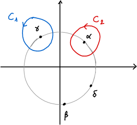
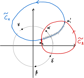
Figure 14: Left: representation of the two contours of integration when $\Sigma$ is the Riemann sphere for the inverse Kasteleyn matrix of Section 6.1. The curve $A_{0}$ is the unit circle in this case. Right: deformation of the contours in the case when the two critical points of $F$ are not on the unit circle (they are thus on different sides), to be in position to apply the saddle point method. Deforming the contours like this creates unwanted contribution to the integral of the residue at $u=v$ along the hatched segment joining the two critical points of $F$, which has to be subtracted.

The corresponding probability of the corresponding edge converges to a number strictly between 0 and 1: we are in the so-called liquid region, or rough phase. On the contrary, when the two critical points are both real, the integral becomes trivial, and the corresponding probability is either 0 or 1: we are then in a frozen region.

The arctic curve describing the transition from the liquid region the a frozen phase is thus given by the set of coordinates $(x,y)$ for which the two critical points merge on the real axis.

In our case, these two critical points merge when $x$ and $y$ satisfy the following equation:

$$r^{2}(x-\frac{1}{2})^{2}+r^{2}(y-\frac{1}{2})^{2}+2r(2-r)(x-\frac{1}{2})(y-\frac{1}{2})=r-1$$

where

$$r=\frac{(\beta-\alpha)(\delta-\gamma)}{(\beta-\gamma)(\delta-\alpha)}=(\alpha,\gamma;\beta,\delta)\in(1,+\infty)$$

is the cross ratio of the four points $\alpha,\gamma,\beta,\delta$.

We know by [KO06] that two sets of isoradial critical weights correspond are gauge equivalent if the corresponding train-track parameters are related by a Möbius transformation preserving the unit circle. The cross-ratio $r$ being Möbius invariant, it is expected that the limit shape if a function of this parameter.

When $r=2$ (for which a representative is when $\alpha$, $\gamma$, $\beta$, $\delta$ cut the unit circle in four equal arcs), the corresponding Boltzmann measure is uniform, and the arctic curve is a circle. A cross-ration $r\neq 2$ can be obtained by putting different weight on NE/SW and NW/SE dominos. Choosing the parameters $\alpha,\gamma,\beta,\delta$ to be $\pm e^{\pm i\theta/2}$, the ratio between the weights is given by $\tan\frac{\theta}{2}$ and $r=(\cos\frac{\theta}{2})^{-2}$. In this case, the arctic curve is an ellipse, as proved by Johansson [Joh02, Theorem 2.4].

Figure 15: Arctic regions for (1-)periodic critical weights, for various values of the cross-ratio $r$ between $\alpha$, $\beta$, $\gamma$ and $\delta$. Here $r=(\cos\frac{\theta}{2})^{-2}$ and $\theta=k\frac{\pi}{20}$ for $k=1,\ldots,10$. The green circle corresponding to the classical arctic circle for the uniform measure, for $k=10$.

6.2 The (periodic) critical Aztec diamond has no gaseous phase

We assume now that the parameters ${\bm{\alpha}},{\bm{\beta}}$ (resp. ${\bm{\gamma}},{\bm{\delta}}$) are periodic with period $l$ (resp. $k$), for some $k,l\geq 1$.

The integrand in the formula describing the probability of a single edge has the same form, as Equation (33), where now the function $F(u;x,y)$ is given by the formula:

$$F(u;x,y)=\frac{1}{l}\sum_{j=1}^{l}\left[y\log(u-\alpha_{j})+(1-y)\log(u-\beta_{j})\right]\\ -\frac{1}{k}\sum_{j=1}^{k}\left[x\log(u-\gamma_{j})+(1-x)\log(u-\delta_{j})\right].$$

The equation for critical points of $F(\cdot;x,y)$ can be rewritten as:

$$\frac{1}{l}\sum_{j=1}^{l}\left[\frac{y}{u-\alpha_{j}}+\frac{1-y}{u-\beta_{j}}\right]=\frac{1}{k}\sum_{j=1}^{k}\left[\frac{x}{u-\gamma_{j}}+\frac{1-x}{u-\delta_{j}}\right],$$

which by putting everything above the same denominator, becomes a polynomial equation in $u$ of degree $2k+2l-2$. It has thus $2k+2l-2$ complex roots, counted with multiplicity.

On the other hand, writing $u=e^{2i\bar{u}},\alpha_{j}=e^{2i\bar{\alpha}_{j}},\ldots$, and using the fact that

$$\frac{2iu}{u-\alpha}=\frac{e^{i(\bar{u}-\bar{\alpha})}}{\sin(\bar{u}-\bar{\alpha})}=i+\cot(\bar{u}-\bar{\alpha}),$$

the same critical equation has the following form:

$$\frac{1}{l}\sum_{j=1}^{l}\left[y\cot(\bar{u}-\bar{\alpha}_{j})+(1-y)\cot(\bar{u}-\bar{\beta}_{j})\right]=-\frac{1}{k}\sum_{j=1}^{k}\left[x\cot(\bar{u}-\bar{\gamma}_{j})+(1-x)\cot(\bar{u}-\bar{\delta}_{j})\right]$$

when $\bar{u}$ is real, both sides are real. The left-hand side takes all real values between $-\infty$ and $+\infty$ when $\bar{u}$ is in $(\bar{\alpha}_{j},\bar{\alpha}_{j+1})$ or $(\bar{\beta}_{j},\bar{\beta}_{j+1})$, for some $1\leq j\leq l-1$, whereas the right-hand side stays bounded on those intervals. As a consequence, there is at least a solution of the critical equation on each of these intervals. Reasoning in the same way on the intervals $(\bar{\gamma}_{j},\bar{\gamma}_{j+1})$, $(\bar{\delta}_{j},\bar{\delta}_{j+1})$, $1\leq j\leq k-1$, exchanging the roles of the left- and right-hand sides, this gives in total at least $2k+2l-4$ real roots. Therefore, there are at most two complex, non-real roots, for the equation in $\bar{u}$, which have to be complex conjugated. This means that for the original equation in $u=e^{2i\bar{u}}$, the two extra solutions are not on the unit circle and the reciprocal of the complex conjugate of one is equal to the other.

Repeating the same saddle-point analysis as above, one can see that the probability of the considered edge, will have a limit, which will be non trivial in $(0,1)$ if and only the two extra critical points are not on the unit circle. When this is the case, let us call $u_{0}$ the one inside the unit disc. Then one sees that we can find a unique point $(x,y)$ which has $u_{0}$ (and the inverse of its complex conjugate) as critical points for $F$, by solving the system of two real linear equations obtained by separating the real and imaginary part of

$$\frac{\partial}{\partial u}F(u_{0};x,y)=0.$$

whereas, the edge will be frozen if all the critical points are real. The argument that this linear system has a unique solution, which is furthermore in the square $[0,1]$ is an slight adaptation of the proof of [BB23, Theorem 4.9].

The transition between the two regimes occur when the two extra complex critical points merge at some $u_{0}=e^{2i\bar{u_{0}}}$ on the unit circle, where they become zeros of the first, and second derivative of $F(\cdot;x,y)$. The arctic curve separating the two regimes is obtained finding $x$ and $y$ such that

$$\begin{cases}\frac{\partial}{\partial u}F(u_{0};x,y)=0\\ \frac{\partial^{2}}{\partial u^{2}}F(u_{0};x,y)=0\end{cases}$$ (34)

for any point $u_{0}$ on the unit circle $S^{1}$. Since $F$ is an affine function of $x$ and $y$, this amounts to solving again a linear system in $x$ and $y$ with coefficients which are explicit functions of $u_{0}$, yielding an explicit parametrization of the arctic curve $u_{0}\in S^{1}\mapsto(x(u_{0}),y(u_{0}))$.

The result above can be summarized in the following proposition:

Proposition 26.

For periodic “genus 0” weights, with arbitrary fundamental domain,

• The map from the unit disc to the liquid region is a homeomorphism.

• the arctic curve has a single component and has an explicit parametrization by trigonometric (or rational) functions. It is thus a real algebraic curve of genus 0. In particular there is no gaseous phase.

• The tangency points with the sides of the of the square $[0,1]$ at the bottom (resp. top, left, right) to $u_{0}$ taking one of the values of ${\bm{\alpha}}$ (resp. ${\bm{\beta}}$, ${\bm{\gamma}}$, ${\bm{\delta}}$).

The genus 0 weights are not generic, and is not covered by the results of Berggren and Borodin [BB23]. The statement about the tangency points has been noticed by Dan Betea for Schur measures corresponding to the Aztec diamond, when parameters are periodic (which is essentially Stanley’s weights in the periodic setting) [Bet15].

The discussion above is mainly about the arctic curve separating the liquid and the frozen region. Actually, the saddle point analysis allows to find the frequency of each type of domino near any point of the liquid region, from which we can reconstruct the expected slope, and then the limit shape.

Figure 16: The arctic curve for critical periodic Aztec diamond (with period 3 vertically, and 2 horizontally).

6.3 The elliptic case

We briefly study here the case of elliptic weights, with periodic train-track parameters. The surface $\Sigma$ is now a torus $\mathbb{C}/(\mathbb{Z}+\tau\mathbb{Z})$ where $\tau\in i\mathbb{R}^{*}_{+}$.

First, as in Section 6.1, let us consider the case where the parameters $\alpha_{j}$ (resp. $\beta_{j}$, $\gamma_{j}$, $\delta_{j}$) are equal to the same value $\alpha$ (resp. $\beta$, $\gamma$, $\delta$) belonging to $\mathbb{R}/\mathbb{Z}$.

Rewriting the probability of a single edge using (25), with the same notation as for the critical case, we get:

$$\mathsf{K}_{\mathsf{w},\mathsf{b}}\mathsf{K}^{-1}_{\mathsf{b},\mathsf{w}}=\int_{\mathscr{C}_{1}}\int_{\mathscr{C}_{2}}\exp(n(F(u;x,y)-F(v;x,y))+o(1))\frac{du\,dv}{\theta_{1}(\pi(v-u))}$$

where now

$$F(u;x,y)=y\log\theta_{1}(\pi(u-\alpha))+(1-y)\log\theta_{1}(\pi(u-\beta))\\ -x\log\theta_{1}(\pi(u-\gamma))-(1-x)\log\theta_{1}(\pi(u-\delta)).$$

The differential of $F$ is a meromorphic 1-form on the torus $\Sigma$. It has a divisor of degree $2g-2=0$. Since $F$ is periodic in the horizontal direction of the torus, the integral of $dF$ along the cycle $\frac{\tau}{2}+\mathbb{R}/\mathbb{Z}$ is equal to 0. Moreover, since $dF$ is real on this cycle, the intermediate value theorem implies that $dF$ has at least two zeros on this cycle. Since it has four simple poles, located at $\alpha$, $\beta$, $\gamma$ and $\delta$, it must have two additional zeros.

These extra zeros can be either both on the same real component of the torus (in a frozen or gaseous phase), or both non-real and symmetric, and complex conjugated (in the liquid phase).

The boundary of the liquid phase is thus obtained by looking at the transition between the two regimes, when the two extra critical points merge into a double critical point. As in the critical case, asking for $u$ to be a double critical point of $F$ yields a linear system in $x$ and $y$ with coefficients that are given in terms of elliptic functions of $u$. When $u$ runs along the two real components of the torus, we get two closed curves: the outer curve separates the liquid phase from the frozen ones in the corners; the inner one separates the liquid phase from the gas bubble near the center.

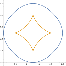
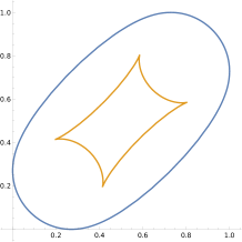
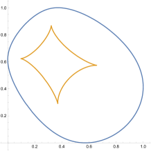
Figure 17: Three arctic curves for a torus with $\tau=i\sqrt{3}$. Left: the limit shape for the unbiased $2\times 2$-periodic Aztec diamond ($\alpha,\beta,\gamma,\delta$ cut the circle into four equal arcs). Center: the limit shape for the biased weights with $\rho=\frac{1}{6}$ ($\alpha=0,\gamma=\frac{1}{6},\beta=\frac{1}{2},\delta=\frac{5}{6}$) and the same value of $\tau$. Right: $\alpha=0,\beta=\frac{3}{5},\gamma=\frac{3}{10},\delta=\frac{17}{20}$

Note that having periodic (even constant here) train-track parameters does not imply that the edge weights are periodic [BCdT23a, Section 4]. In order for the edge weights to be periodic, for a fundamental domain containing two white and two black vertices, the parameters $\alpha,\beta,\gamma,\delta$ should satisfy:

$$\alpha-\beta+\gamma-\delta=0\text{ mod }1,\qquad\alpha-\beta-\gamma+\delta=0\text{ mod }1.$$ (35)

which means that $\beta-\alpha=\pm\frac{1}{2}$, and $\delta-\gamma=\pm\frac{1}{2}$. This case contains in particular the $2\times 2$ periodic Aztec diamond, studied by

• Chhita and Johansson [CJ16] by taking $\alpha=0,\beta=\frac{1}{2},\gamma=\frac{1}{4},\delta=\frac{3}{4}$ and letting $\tau$ vary on the imaginary axis,

• Borodin and Duits [BD23], for a specific value of $t$, which in fact does not play a role in the computation of the limit shape.

These are the cases depicted on the left and middle of Figure 17. An example where the periodicity condition is not satisfied is shown on the right of that same figure. Note that in this case, the picture does not have axial symmetries anymore.

One can extend this study when the parameters ${\bm{\alpha}}$, ${\bm{\beta}}$, ${\bm{\gamma}}$, and ${\bm{\delta}}$ are $k\times l$ period, like in Section 6.2. With the additional constraint that the corresponding edge weights are periodic, this covers in particular the case $k=2,l=2$ in the study of Berggren and Borodin [BB23] (without the technical assumption they have on the weights to guarantee that the vertical tentacles of the amoeba of the corresponding spectral curve are separated), but also the extension to the case where the periodicity condition for edge weights is not met, like the one depicted on Figure 18. One can relate here, like in the critical case, the number of cusps along bottom, left, top, right side of the square with the number of distinct values for ${\bm{\alpha}}$, ${\bm{\gamma}}$, ${\bm{\beta}}$, ${\bm{\delta}}$ respectively, whereas there are four of them along the liquid/gas interface.

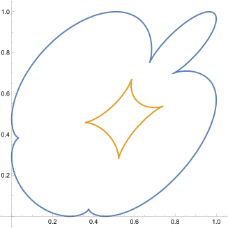
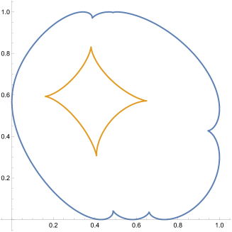
Figure 18: Left: a 2x2 example with ${\bm{\alpha}}=\{0.744904,0.448131\}$, ${\bm{\beta}}=\{2.35367,1.58096\}$, ${\bm{\gamma}}=\{1.21721,0.983251\}$, ${\bm{\delta}}=\{3.05117,2.38214\}$. Right: a 3x2 example where ${\bm{\alpha}}=\{0.599648,0.0928766,0.288755\}$, ${\bm{\beta}}=\{2.29566,1.7928,2.20249\}$, ${\bm{\gamma}}=\{1.18328\}$, ${\bm{\delta}}=\{3.06226,2.74699\}$. The fact that there is a single contact point on the left boundary (whereas there are two on the right side) is a consequence of the fact that ${\bm{\gamma}}$ is 1-periodic (constant) whereas ${\bm{\delta}}$ is 2-periodic.

6.4 Higher genus

The study above can be done on surfaces with higher genus, with train-track parameters assigned in a periodic way, even though it can be technically challenging to work with prime forms to control the saddle point method. Imposing periodicity for weights from periodicity of train-track parameters implies that the fundamental domain is large enough (one needs to pick $g$ distinct integer points in the interior points of the corresponding Newton polygon), but we can relax this condition (and get just quasi-periodic weights), as in the genus 1 case above.

In [BB23], the authors give a similar looking formula for the inverse of the Kasteleyn matrix of the Aztec diamond with periodic weights. The main differences are the fact that the integrals are written with respect to the coordinates $z$ (and $w$) of the spectral curve instead of an intrisic coordinate of the Riemann surface $\Sigma$, and the fact that the integrand is a block matrix. Otherwise, unsurprisingly, the function $F$ appearing in the asymptotics of the integral is the same as here. We refer to the paper [BB23] for a detailed discussion of the saddle point method in the periodic case under additional technical assumptions. Working with formula (17) can be seen as a way to circumvent the technical assumptions they have to extend their results to non-generic cases, where the spectral curve is singular or the amoeba has a degenerate behaviour. In that case, the geometric correspondence is to be made between the limit shape of the Aztec diamond and the “upper part” $\Sigma^{+}$ of $\Sigma$, which is the connected component of $\Sigma\setminus\bigcup_{i=0}^{g}A_{i}$ whose oriented boundary is $A_{0}-\sum_{i=1}^{g}A_{i}$ (instead of the amoeba of the spectral curve). Most of their geometric arguments can be carried or adapted in this slightly changed context to obtain the following:

Proposition 27 ([BB23]).

• The map $\psi$ from $(x,y)$ in the liquid region to the critical point of $F$ in the interior of $\Sigma^{+}$ is a homeomorphism.

• There is a bijective correspondence between gaseous bubbles and the real ovals $A_{1},\cdots A_{g}$.

• There is a bijective correspondence between frozen regions and connected components of $A_{0}\setminus\{\alpha_{j},\beta_{j},\gamma_{j},\delta_{j}\ ;\ 1\leq j\leq n\}$.

The saddle point method allows one to not only compute the probability that a given edge occurs, but also to derive the asymptotics for the entry of inverse Kasteleyn matrix for vertices $\mathsf{b}$ and $\mathsf{w}$ at finite distance, near the same macroscopic point $(x,y)$ in the liquid region: it converges to $A^{u_{0}}_{\mathsf{b},\mathsf{w}}$, where $u_{0}=\psi(x,y)$ is the critical point of $F(\cdot;x,y)$ in $\Sigma^{+}$, and $A^{u_{0}}$ is the inverse from the family of inverses introduced in [BCdT23a] for the Fock Kasteleyn operator on any infinite minimal graph containing as a subgraph a neighborhood of the Aztec diamond containing $\mathsf{w}$ and $\mathsf{b}$ (for example the infinite square lattice). The inverse $A^{u_{0}}$ on the infinite square defines a Gibbs measure $\mathbb{P}^{u_{0}}$ on dimer configurations by the usual determinantal formula:

$$\mathbb{P}^{u_{0}}((\mathsf{w}_{1},\mathsf{b}_{1}),\dots,(\mathsf{w}_{k},\mathsf{b}_{k}))=\Bigl{(}\prod_{j=1}^{k}\mathsf{K}_{\mathsf{w}_{j},\mathsf{b}_{j}}\Bigr{)}\det_{1\leq i,j\leq k}\left(A^{u_{0}}_{\mathsf{b}_{i},\mathsf{w}_{j}}\right)$$

Therefore, one can obtain in this generalized setup the analogue of [BB23, Theorem 1.10]:

Proposition 28.

The local statistics of dimers around a point $(x,y)$ of the liquid region converge to the infinite Gibbs measure $\mathbb{P}^{u_{0}}$ on the square lattice, with $u_{0}=\psi(x,y)$.

We also note that the imaginary part of the equation used to determine the critical points of $F$, is the same as the master equation for the tangent plane method by Kenyon and Prause [KP22b, KP22a, KP24]: indeed, for a fixed $u$, the action $F$ is an affine function of $x$ and $y$, and the coefficients of $x$ and $y$ (respectively $\log z(u)$ and $\log w(u)$) which are analytic functions of $u$, and whose imaginary parts give the slope of the limit shape at the point $(x,y)$, see [BCdT23a, Section 4.5]. The remaining constant part is encoding the boundary conditions and should be directly related to the intercept function. We have thus two interpretations of the same equation: one coming from finding critical points of the action functional $F$, the other other one by looking at isothermal coordinates in which the slope and the intercept of the asymptotic height function describing the limit shape are harmonic. Further investigation is needed to make a full connection between the two approaches. A starting point is the expression of the expression of the surface tension in terms of geometric quantities on $\Sigma$, obtained in [BCdT23a, Section 4.6], see also [BBS].

References

- [BB23] Tomas Berggren and Alexei Borodin. Geometry of the doubly periodic aztec dimer model, 2023.
- [BBC+17] Cédric Boutillier, Jérémie Bouttier, Guillaume Chapuy, Sylvie Corteel, and Sanjay Ramassamy. Dimers on rail yard graphs. Ann. Inst. Henri Poincaré D, 4(4):479–539, 2017.
- [BBS] Alexander I. Bobenko, Nikolai Bobenko, and Yuri B. Suris. Limit shape for domino and lozenge tilings with Focks’ weights. In preparation.
- [BCdT22] Cédric Boutillier, David Cimasoni, and Béatrice de Tilière. Isoradial immersions. Journal of Graph Theory, 99(4):715–757, 2022.
- [BCdT23a] Cédric Boutillier, David Cimasoni, and Béatrice de Tilière. Minimal bipartite dimers and higher genus harnack curves. Probability and Mathematical Physics, 4(1):151–208, March 2023.
- [BCdT23b] Cédric Boutillier, David Cimasoni, and Béatrice de Tilière. Elliptic dimer models on minimal graphs and genus 1 harnack curves. Communications in Mathematical Physics, 400(2):1071–1136, February 2023.
- [BD19] Tomas Berggren and Maurice Duits. Correlation functions for determinantal processes defined by infinite block toeplitz minors. Advances in Mathematics, 356:106766, 2019.
- [BD23] Alexei Borodin and Maurice Duits. Biased 2 2 periodic Aztec diamond and an elliptic curve. Probability Theory and Related Fields, pages 1–57, 2023.
- [Ber21] Tomas Berggren. Domino tilings of the aztec diamond with doubly periodic weightings. Ann. Probab., 49(4):1965–2011, 2021.
- [Bet15] Dan Betea. private communication. https://icerm.brown.edu/materials/Slides/sp-s15-w3/Limit_shapes_in_the_Schur_process_]_Dan_Betea,_Universit%C3%A9_de_Paris_VI_(Pierre_et_Marie_Curie).pdf, 2015.
- [CJ16] Sunil Chhita and Kurt Johansson. Domino statistics of the two-periodic Aztec diamond. Adv. Math., 294:37–149, 2016.
- [CJY15] Sunil Chhita, Kurt Johansson, and Benjamin Young. Asymptotic domino statistics in the Aztec diamond. Ann. Appl. Probab., 25(3):1232–1278, 2015.
- [CKP01] Henry Cohn, Richard Kenyon, and James Propp. A variational principle for domino tilings. J. Amer. Math. Soc., 14(2):297–346 (electronic), 2001.
- [CY14] Sunil Chhita and Benjamin Young. Coupling functions for domino tilings of Aztec diamonds. Adv. Math., 259:173–251, 2014.
- [DFSG14] Philippe Di Francesco and Rodrigo Soto-Garrido. Arctic curves of the octahedron equation. J. Phys. A, Math. Theor., 47(28):34, 2014. Id/No 285204.
- [DK21] Maurice Duits and Arno B. J. Kuijlaars. The two-periodic Aztec diamond and matrix valued orthogonal polynomials. J. Eur. Math. Soc. (JEMS), 23(4):1075–1131, 2021.
- [DLMF] NIST Digital Library of Mathematical Functions. https://dlmf.nist.gov/, Release 1.2.0 of 2024-03-15. F. W. J. Olver, A. B. Olde Daalhuis, D. W. Lozier, B. I. Schneider, R. F. Boisvert, C. W. Clark, B. R. Miller, B. V. Saunders, H. S. Cohl, and M. A. McClain, eds.
- [Dob68] Roland L. Dobrušin. Description of a random field by means of conditional probabilities and conditions for its regularity. Teor. Verojatnost. i Primenen, 13:201–229, 1968.
- [EKLP92] Noam Elkies, Greg Kuperberg, Michael Larsen, and James Propp. Alternating-sign matrices and domino tilings (part I). Journal of Algebraic Combinatorics, 1:111–132, 1992.
- [Fay73] John D. Fay. Theta functions on Riemann surfaces., volume 352. Springer, Cham, 1973.
- [Foc15] Vladimir V. Fock. Inverse spectral problem for GK integrable system. arXiv e-prints, page arXiv:1503.00289, March 2015.
- [GK13] Alexander B. Goncharov and Richard Kenyon. Dimers and cluster integrable systems. Ann. Sci. Éc. Norm. Supér., 46(5):747–813, 2013.
- [Hel00] Harald Helfgott. Edge effects on local statistics in lattice dimers: A study of the aztec diamond (finite case), 2000.
- [Joh02] Kurt Johansson. Non-intersecting paths, random tilings and random matrices. Probab. Theory Relat. Fields, 123(2):225–280, 2002.
- [JPS98] William Jokusch, James Propp, and Peter Shor. Random Domino Tilings and the Arctic Circle Theorem, 1998.
- [Kas61] Pieter W. Kasteleyn. The statistics of dimers on a lattice: I. the number of dimer arrangements on a quadratic lattice. Physica, 27:1209–1225, December 1961.
- [Ken97] Richard Kenyon. Local statistics of lattice dimers. Ann. Inst. H. Poincaré Probab. Statist., 33(5):591–618, 1997.
- [Ken02] Richard Kenyon. The Laplacian and Dirac operators on critical planar graphs. Invent. Math., 150(2):409–439, 2002.
- [KO06] Richard Kenyon and Andrei Okounkov. Planar dimers and Harnack curves. Duke Math. J., 131(3):499–524, 2006.
- [KOS06] Richard Kenyon, Andrei Okounkov, and Scott Sheffield. Dimers and amoebae. Ann. of Math. (2), 163(3):1019–1056, 2006.
- [KP22a] Richard Kenyon and István Prause. The genus-zero five-vertex model. Probab. Math. Phys., 3(4):707–729, 2022.
- [KP22b] Richard Kenyon and István Prause. Gradient variational problems in . Duke Math. J., 171(14):3003–3022, 2022.
- [KP24] Richard Kenyon and István Prause. Limit shapes from harmonicity: dominos and the five vertex model. J. Phys. A, Math. Theor., 57(3):16, 2024. Id/No 035001.
- [Kuc17] Nikolai Kuchumov. Limit shapes for the dimer model, 2017.
- [Kup98] Greg Kuperberg. An exploration of the permanent-determinant method. Electron. J. Combin., 5:Research Paper 46, 34, 1998.
- [Law89] Derek F. Lawden. Elliptic functions and applications, volume 80 of Applied Mathematical Sciences. Springer-Verlag, New York, 1989.
- [LIR69] Oscar E. Lanford III and David Ruelle. Observables at infinity and states with short range correlations in statistical mechanics. Comm. Math. Phys., 13:194–215, 1969.
- [Mum07] David Mumford. Tata lectures on theta. II. Modern Birkhäuser Classics. Birkhäuser Boston, Inc., Boston, MA, 2007. Jacobian theta functions and differential equations, With the collaboration of C. Musili, M. Nori, E. Previato, M. Stillman and H. Umemura, Reprint of the 1984 original.
- [OR03] A. Okounkov and N. Reshetikhin. Correlation function of schur process with application to local geometry of a random 3-dimensional young diagram. J. Amer. Math. Soc., 16(3):581–603, 2003.
- [Per69] Jerome K. Percus. One more technique for the dimer problem. J. Math. Phys., 10:1881, 1969.
- [Pro97] James Propp. Talk given at the American Mathematical Society meeting in San Diego. Slides available at http://jamespropp.org/san_diego.pdf, 1997.
- [Pro03] James Propp. Generalized domino-shuffling. Theoret. Comput. Sci., 303(2-3):267–301, 2003. Tilings of the plane.
- [Spe07] David E. Speyer. Perfect matchings and the octahedron recurrence. J. Algebr. Comb., 25(3):309–348, 2007.
- [TF61] Harold N. V. Temperley and Michael E. Fisher. Dimer problem in statistical mechanics-an exact result. Philosophical Magazine, 6(68):1061–1063, 1961.
- [Thu90] William P. Thurston. Conway’s tiling groups. Amer. Math. Monthly, 97(8):757–773, 1990.
- [Thu17] Dylan P. Thurston. From dominoes to hexagons. In Proceedings of the 2014 Maui and 2015 Qinhuangdao conferences in honour of Vaughan F. R. Jones’ 60th birthday, volume 46 of Proc. Centre Math. Appl. Austral. Nat. Univ., pages 399–414. Austral. Nat. Univ., Canberra, 2017.
- [Yan91] Bo-Yin Yang. Two enumeration problems about the Aztec diamonds. ProQuest LLC, Ann Arbor, MI, 1991. Thesis (Ph.D.)–Massachusetts Institute of Technology, available online at http://hdl.handle.net/1721.1/13937.