Pre-train and Refine: Towards Higher Efficiency in K-Agnostic Community Detection without Quality Degradation

Abstract.

Community detection (CD) is a classic graph inference task that partitions nodes of a graph into densely connected groups. While many CD methods have been proposed with either impressive quality or efficiency, balancing the two aspects remains a challenge. This study explores the potential of deep graph learning to achieve a better trade-off between the quality and efficiency of $K$-agnostic CD, where the number of communities $K$ is unknown. We propose PRoCD (Pre-training & Refinement for Community Detection), a simple yet effective method that reformulates $K$-agnostic CD as the binary node pair classification. PRoCD follows a pre-training & refinement paradigm inspired by recent advances in pre-training techniques. We first conduct the offline pre-training of PRoCD on small synthetic graphs covering various topology properties. Based on the inductive inference across graphs, we then generalize the pre-trained model (with frozen parameters) to large real graphs and use the derived CD results as the initialization of an existing efficient CD method (e.g., InfoMap) to further refine the quality of CD results. In addition to benefiting from the transfer ability regarding quality, the online generalization and refinement can also help achieve high inference efficiency, since there is no time-consuming model optimization. Experiments on public datasets with various scales demonstrate that PRoCD can ensure higher efficiency in $K$-agnostic CD without significant quality degradation.

1. Introduction

Community detection (CD) is a classic graph inference task that partitions nodes of a graph into several groups (i.e., communities) with dense linkage distinct from other groups (Fortunato and Newman, 2022). It has been validated that the extracted communities may correspond to substructures of various real-world complex systems (e.g., functional groups in protein interactions (Fortunato, 2010)). Many network applications (e.g., cellular network decomposition (Dai and Bai, 2017) and Internet traffic profiling (Qin et al., 2019)) are thus formulated as CD. Due to the NP-hardness of some typical CD objectives (e.g., modularity maximization (Newman, 2006)), balancing the quality and efficiency of CD on large graphs remains a challenge. Most existing approaches focus on either high quality or efficiency.

On the one hand, efficient CD methods usually adopt heuristic strategies or fast approximation w.r.t. some relaxed CD objectives to obtain feasible CD results (e.g., the greedy maximization (Blondel et al., 2008) and semi-definite relaxation (Wang and Kolter, 2020) of modularity). Following the graph embedding framework, which maps nodes $\mathcal{V}=\{v_{i}\}$ of a graph into low-dimensional vector representations $\{{\bf{z}}_{i}\in\mathbb{R}^{d}\}$ ($d\ll|\mathcal{V}|$) with major topology properties preserved, several efficient embedding approaches have also been proposed based on approximated dimension reduction (e.g., random projection for high-order topology (Zhang et al., 2018)). Some of them are claimed to be community-preserving and able to support CD using a downstream clustering module (Bhowmick et al., 2020; Gao et al., 2023). Despite the high efficiency, these methods may potentially suffer from quality degradation due to the information loss of heuristics, approximation, and relaxation.

On the other hand, recent studies have demonstrated the ability of deep graph learning (DGL) techniques (Rong et al., 2020; Zhang et al., 2020), e.g., those based on graph neural networks (GNNs), to achieve impressive quality of various graph inference tasks including CD (Xing et al., 2022). However, their powerful performance usually relies on iterative optimization algorithms (e.g., gradient descent) that direct sophisticated models to fit complicated objectives, which usually have high complexities.

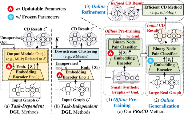
Figure 1. Overview of mainstream (a) task-dependent and (b) -independent DGL methods as well as (c) our PRoCD method.

In this study, we explore the potential of DGL to ensure higher efficiency in CD without significant quality degradation, compared with mainstream efficient and DGL methods. It serves as a possible way to achieve a better trade-off between the two aspects. Different from existing CD methods (Dhillon et al., 2007; Chen et al., 2019; Tsitsulin et al., 2023) with an assumption that the number of communities $K$ is given, we consider the more challenging yet realistic $K$-agnostic CD, where $K$ is unknown. In this setting, one should simultaneously determine $K$ and the corresponding community partition.

Dilemmas. As shown in Fig. 1 (a) and (b), existing DGL-based CD techniques usually follow the unified graph embedding framework and can be categorized into the (i) task-dependent and (ii) task-independent approaches. We argue that they may suffer from the following limitations w.r.t. our settings.

First, existing DGL methods may be inapplicable to $K$-agnostic CD. Given a graph $\mathcal{G}$, some task-dependent approaches (Wilder et al., 2019; Chen et al., 2019; Tsitsulin et al., 2023) (see Fig. 1 (a)) generate embeddings $\{{\bf{z}}_{i}\}$ via an embedding encoder ${\mathop{\rm Enc}\nolimits}(\cdot)$ (e.g., a multi-layer GNN) and feed $\{{\bf{z}}_{i}\}$ into an output module ${\mathop{\rm Out}\nolimits}(\cdot)$ (e.g., a multi-layer perceptron (MLP)) to derive the CD result $\mathcal{C}$, i.e., $\{{{\bf{z}}_{i}}\}={\mathop{\rm Enc}\nolimits}(\mathcal{G})$ and $\mathcal{C}={\mathop{\rm Out}\nolimits}(\{{{\bf{z}}_{i}}\})$. Since parameters in ${\mathop{\rm Out}\nolimits}(\cdot)$ are usually with the dimensionality related to $K$, these task-dependent methods cannot output a feasible CD result when $K$ is unknown. Although some task-independent methods (Yang et al., 2016; Liu et al., 2022; Qin et al., 2023b) (see Fig. 1 (b)) do not contain ${\mathop{\rm Out}\nolimits}(\cdot)$ related to $K$, their original designs still rely on a downstream clustering algorithm (e.g., $K$Means) with $\{{\bf{z}}_{i}\}$ and $K$ as required inputs.

Second, the standard transductive inference of some DGL techniques may result in low efficiency. As illustrated in Fig. 1 (a) and (b), during the inference of CD on each single graph, these transductive methods must first optimize their model parameters from scratch via unsupervised objectives, which is usually time-consuming. Some related studies (Yang et al., 2016; Liu et al., 2022; Tsitsulin et al., 2023) only consider transductive inference regardless of its low efficiency.

Focusing on the CD with a given $K$ and task-independent architecture in Fig. 1 (b), recent research (Qin et al., 2023b) has validated that the inductive inference, which (i) trains a DGL model on historical graphs $\{{\mathcal{G}}_{t}\}$ and (ii) generalizes it to new graphs $\{\mathcal{G}^{\prime}\}$ without additional optimization, can help achieve high inference efficiency on $\{\mathcal{G}^{\prime}\}$. One can extend this method to $K$-agnostic CD by replacing the downstream clustering module (e.g., $K$Means) with an advanced algorithm unrelated to $K$ (e.g., DBSCAN (Schubert et al., 2017)). Our experiments indicate that such a naive extension may still have low inference quality and efficiency compared with conventional baselines.

Contributions. We propose PRoCD (Pre-training & Refinement for Community Detection), a simple yet effective method as illustrated in Fig. 1 (c), to address the aforementioned limitations.

A novel model architecture. To derive feasible results for $K$-agnostic CD in an end-to-end way, we reformulate CD as the binary node pair classification. Unlike existing end-to-end models that directly assign the community label $c_{i}\in\{1,\cdots,K\}$ of each node $v_{i}$ (e.g., via an MLP in Fig. 1 (a)), we develop a binary classifier, with a new design of pair-wise temperature parameters, to determine whether a pair of nodes $(v_{i},v_{j})$ are partitioned into the same community. Given the classification result w.r.t. a set of node pairs $\mathcal{P}=\{(v_{i},v_{j})\}$ sampled from a graph $\mathcal{G}$, we construct another auxiliary graph $\mathcal{\tilde{G}}$, from which a feasible CD result of $\mathcal{G}$ can be extracted. Each connected component in $\mathcal{\tilde{G}}$ corresponds to a community in $\mathcal{G}$, with the number of components as the estimated $K$.

A novel learning paradigm. Inspired by recent advances in graph pre-training techniques, PRoCD follows a novel pre-training & refinement paradigm with three phases as in Fig. 1 (c). Based on the assumption that one has enough time to prepare a well-trained model in an offline way (i.e., offline pre-training), we first pre-train PRoCD on small synthetic graphs with various topology properties (e.g., degree distributions) and high-quality community ground-truth. We then generalize PRoCD (with frozen parameters) to large real graphs $\{\mathcal{G}^{\prime}\}$ (i.e., online generalization) and derive corresponding CD results $\{\mathcal{\bar{C}^{\prime}}\}$ via only one feed-forward propagation (FFP) of the model (i.e., inductive inference of DGL). In some pre-training techniques (Wu et al., 2021; Sun et al., 2023b), online generalization only provides an initialization of model parameters, which is further fine-tuned w.r.t. different tasks. Analogous to this motivation, we treat $\mathcal{\bar{C}^{\prime}}$ as the initialization of an efficient CD method (e.g., InfoMap (Rosvall and Bergstrom, 2008)) and adopt its output $\mathcal{C}^{\prime}$ as the final CD result, which refines $\mathcal{\bar{C}^{\prime}}$ (i.e., online refinement). In particular, the online generalization and refinement may benefit from the powerful transfer ability of inductive inference regarding quality while ensuring high inference efficiency, since there is no time-consuming model optimization.

Note that our pre-training & refinement paradigm is different from existing graph pre-training techniques (Wu et al., 2021; Sun et al., 2023b). We argue that they may suffer from the following issues about CD. Besides pre-training, these methods may require another optimization procedure for the fine-tuning or prompt-tuning of specific tasks on $\{\mathcal{G}^{\prime}\}$, which is time-consuming and thus cannot help achieve high efficiency on $\{\mathcal{G}^{\prime}\}$. To the best of our knowledge, related studies (Liu et al., 2023; Cao et al., 2023; Sun et al., 2023a) merely focus on supervised tasks (e.g., node classification) and do not provide unsupervised tuning objectives for CD.

A better trade-off between quality and efficiency. Experiments on datasets with various scales demonstrate that PRoCD can ensure higher inference efficiency in CD without significant quality degradation, compared with running a refinement method from scratch. In some cases, PRoCD can even achieve improvement in both aspects. Therefore, we believe that this study provides a possible way to obtain a better trade-off between the two aspects.

Table 1. Summary of some representative CD methods.

Methods

FastCom

GraClus

MC-SBM

Par-SBM

GMod

LPA

InfoMap

Louvain

Locale

ClusNet

LGNN

GAP

DMoN

DNR

DCRN

ICD

References

(Clauset et al., 2004)

(Dhillon et al., 2007)

(Peixoto, 2014)

(Peng et al., 2015)

(Clauset et al., 2004)

(Raghavan et al., 2007)

(Rosvall and Bergstrom, 2008)

(Blondel et al., 2008)

(Wang and Kolter, 2020)

(Wilder et al., 2019)

(Chen et al., 2019)

(Nazi et al., 2019)

(Tsitsulin et al., 2023)

(Yang et al., 2016)

(Liu et al., 2022)

(Qin et al., 2023b)

Focus

High Efficiency

High Quality

Q&E

Techniques

Heuristic strategies or fast approximation w.r.t. relaxed CD objectives

Task-dependent DGL

Task-independent DGL

Inference

Running the algorithm from scratch for each graph

Transductive & Inductive

Transductive

Inductive

$K$-agnostic

2718

2718

2714

2714

2714

2714

2714

2714

2714

2718

2718

2718

2718

2718

2718

2718

2. Related Work

In the past few decades, many CD methods have been proposed based on different problem statements, hypotheses, and techniques (Xing et al., 2022). Table 1 summarizes some representative approaches according to their original designs. Most of them focus on either high efficiency or quality. Conventional efficient CD methods use heuristic strategies or fast approximation w.r.t. some relaxed CD objectives to derive feasible CD results, including the (i) greedy modularity maximization in FastCom (Clauset et al., 2004) and Louvain (Blondel et al., 2008), (ii) semi-definite relaxation of modularity in Locale (Wang and Kolter, 2020), (iii) label propagation heuristic in LPA (Raghavan et al., 2007), as well as (iv) Monte Carlo approximation of stochastic block model (SBM) in MC-SBM (Peixoto, 2014) and Par-SBM (Peng et al., 2015).

Recent studies have also demonstrated the powerful potential of DGL to ensure high quality of CD, following the architectures in Fig. 1 (a) and (b). However, some methods (e.g., DNR (Yang et al., 2016), DCRN (Liu et al., 2022), and DMoN (Tsitsulin et al., 2023)) only considered the inefficient transductive inference, with time-consuming model optimization in the inference of CD on each single graph. Other approaches (e.g., ClusNet (Wilder et al., 2019), LGNN (Chen et al., 2019), GAP (Nazi et al., 2019), and ICD (Qin et al., 2023b)) considered inductive inference across graphs. Results of ICD validated that the inductive inference can help achieve a better trade-off between quality and efficiency in online generalization (i.e., directly generalizing a model pre-trained on historical graphs $\{\mathcal{G}_{t}\}$ to new graphs $\{\mathcal{G}^{\prime}\}$). Nevertheless, the quality of online generalization may be affected by the possible distribution shift between $\{\mathcal{G}_{t}\}$ and $\{\mathcal{G}^{\prime}\}$. In contrast, online generalization is used to construct the initialization of online refinement in our PRoCD method, which can ensure better quality on $\{\mathcal{G}^{\prime}\}$. Moreover, most task-dependent DGL methods (e.g., ClusNet, LGNN, GAP, and DMoN) are inapplicable to $K$-agnostic CD, since they usually contain an output module related to $K$. Although task-independent approaches (e.g., DNR, DCRN, and ICD) do not contain such a module, their original designs still rely on a pre-set $K$ (e.g., $K$Means as the downstream clustering algorithm).

Different from the aforementioned methods, our PRoCD method can ensure higher efficiency in $K$-agnostic CD without significant quality degradation via a novel model architecture following the pre-training & refinement paradigm, as highlighted in Fig. 1 (c).

As reviewed in (Wu et al., 2021; Sun et al., 2023b), existing graph pre-training techniques usually follow the paradigms of (i) pre-training & fine-tuning (e.g., GCC (Qiu et al., 2020), L2P-GNN (Lu et al., 2021), and W2P-GNN (Cao et al., 2023)) as well as (ii) pre-training & prompting (e.g., GPPT (Sun et al., 2022), GraphPrompt (Liu et al., 2023), and ProG (Sun et al., 2023a)). In addition to offline pre-training, these methods rely on another optimization procedure for the fine-tuning or prompt-tuning of specific inference tasks, which is usually time-consuming. Moreover, most of them merely focus on supervised tasks (e.g., node classification, link prediction, and graph classification) and do not provide unsupervised tuning objectives for CD. Therefore, one cannot directly apply these pre-training methods to ensure the high efficiency in CD without quality degradation.

3. Problem Statements & Preliminaries

In this study, we consider the disjoint CD on undirected graphs. A graph can be represented as $\mathcal{G}=(\mathcal{V},\mathcal{E})$, with $\mathcal{V}=\{v_{1},\cdots,v_{N}\}$ and $\mathcal{E}=\{(v_{i},v_{j})|v_{i},v_{j}\in\mathcal{V})\}$ as the sets of nodes and edges. The topology of $\mathcal{G}$ can be described by an adjacency matrix ${\bf{A}}\in\{0,1\}^{N\times N}$, where ${\bf{A}}_{ij}={\bf{A}}_{ji}=1$ if $(v_{i},v_{j})\in\mathcal{E}$ and ${\bf{A}}_{ij}={\bf{A}}_{ji}=0$ otherwise. Since CD is originally defined only based on graph topology (Fortunato and Newman, 2022), we assume that graph attributes are unavailable.

Community Detection (CD). Given a graph $\mathcal{G}$, CD aims to partition the node set $\mathcal{V}$ into $K$ subsets (defined as communities) ${\mathcal{C}}=\{\mathcal{C}_{1},\cdots,\mathcal{C}_{K}\}$ (${C_{r}}\cap{C_{s}}=\emptyset$ for $\forall r\neq s$) s.t. (i) the linkage within each community is dense but (ii) that between communities is relatively loose. We define that a CD task is $K$-agnostic if the number of communities $K$ is unknown for a given graph $\mathcal{G}$, where one should simultaneously determine $K$ and the corresponding CD result $\mathcal{C}$. We consider $K$-agnostic CD in this study. Whereas, some existing methods (Dhillon et al., 2007; Wilder et al., 2019; Tsitsulin et al., 2023) assume that $K$ is given for each input ${\mathcal{G}}$ and thus cannot tackle such a challenging yet realistic setting.

Modularity Maximization. Mathematically, CD can be formulated as the modularity maximization objective (Newman, 2006), which maximizes the difference between the exact graph topology (described by ${\bf{A}}$) and a randomly generated case. Given $\mathcal{G}$ and $K$, it aims to derive a partition $\mathcal{C}$ that maximizes the following modularity metric:

(1) $$\mathop{\max}\limits_{\mathcal{C}}{\mathop{\rm Mod}\nolimits}(\mathcal{G},K):=\frac{1}{{2M}}\sum\limits_{r=1}^{K}{\sum\limits_{{v_{i}},{v_{j}}\in{\mathcal{C}_{r}}}{[{{\bf{A}}_{ij}}-\frac{{{{\deg}(v_{i})}{{\deg}(v_{j})}}}{{2M}}]}},$$

where $\deg(v_{i})$ is the degree of node $v_{i}$; $M$ is the number of edges. Objective (1) can be rewritten into the following matrix form:

(2) $$\mathop{\min}\limits_{\bf{H}}-{\mathop{\rm tr}\nolimits}({{\bf{H}}^{T}}{\bf{QH}}){\rm{~{}s.t.~{}}}{{\bf{H}}_{ir}}=\left\{{\begin{array}[]{*{20}{l}}{1,~{}{v_{i}}\in{C_{r}}}\\ {0,~{}{\rm{otherwise}}}\end{array}}\right.,$$

where ${\bf{Q}}\in\mathbb{R}^{N\times N}$ is defined as the modularity matrix with ${{\bf{Q}}_{ij}}:=[{{\bf{A}}_{ij}}-{{\deg}(v_{i})}{{\deg}(v_{j})}/(2M)]$; ${\bf{H}}\in\{0,1\}^{N\times K}$ indicates the community membership of $\mathcal{C}$. Our method does not directly solve the aforementioned problem. Instead, we try to extract informative community-preserving features from ${\bf{Q}}$.

Pre-training & Refinement Paradigm. To achieve a better trade-off between the quality and efficiency, we propose a pre-training & refinement paradigm based on the inductive inference of DGL. We represent a DGL model as $\mathcal{C}=f(\mathcal{G};\Theta)$, which derives the CD result $\mathcal{C}$ given a graph $\mathcal{G}$, with $\Theta$ as the set of trainable model parameters. As in Fig. 1 (c), the proposed paradigm includes (i) offline pre-training, (ii) online generalization, and (iii) online refinement.

In offline pre-training, we first generate a set of synthetic graphs $\mathcal{T}=\{\mathcal{G}_{1},\cdots,\mathcal{G}_{T}\}$ via a generator (e.g., SBM (Karrer and Newman, 2011)). The generation of each graph $\mathcal{G}_{t}\in\mathcal{T}$ includes the topology $(\mathcal{V}_{t},\mathcal{E}_{t})$ and community assignment ground-truth $\mathcal{C}^{(t)}$. We then pre-train $f$ on $\mathcal{T}$ (i.e., updating $\Theta$) based on an objective regarding $\{(\mathcal{V}_{t},\mathcal{E}_{t})\}$ and $\{\mathcal{C}^{(t)}\}$ in an offline way. After that, we generalize $f$ to a large real graph $\mathcal{G}^{\prime}$ with frozen $\Theta$ (i.e., online generalization), which can derive a feasible CD result $\mathcal{\bar{C}}^{\prime}$ via only one FFP of $f$ (i.e., inductive inference). Analogous to the fine-tuning in existing pre-training techniques, we treat $\mathcal{\bar{C}}^{\prime}$ as the initialization of a conventional efficient CD method (e.g., InfoMap (Rosvall and Bergstrom, 2008)) and adopt its output $\mathcal{C}^{\prime}$ as the final CD result, which further refines $\mathcal{\bar{C}}^{\prime}$ (i.e., online refinement).

Evaluation Protocol. In real applications, it is usually assumed that one has enough time to prepare a well-trained model in an offline way (e.g., pre-training of LLMs). After deploying $f$, one may achieve high efficiency in the online inference on graphs $\{\mathcal{G}^{\prime}\}$ (e.g., via one FFP of $f$ without any model optimization). In contrast, conventional methods cannot benefit from pre-training but have to run their algorithms on $\{\mathcal{G}^{\prime}\}$ from scratch, due to the inapplicability to inductive inference. Our evaluation focuses on the online inference of CD on $\{\mathcal{G}^{\prime}\}$ (e.g., online generalization and refinement of PRoCD), which is analogous to the applications of foundation models. For instance, users benefit from the powerful online inference of LLMs (e.g., generating high-quality answers in few seconds) but do not need to train them using a great amount of resources.

4. Methodology

We propose PRoCD following a novel pre-training & refinement paradigm as highlighted in Fig. 1 (c).

4.1. Model Architecture

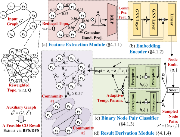
Figure 2. Overview of the model architecture of PRoCD.

To enable PRoCD to derive feasible results for $K$-agnostic CD in an end-to-end architecture, we reformulate CD as the binary node pair classification. For each graph $\mathcal{G}=(\mathcal{V},\mathcal{E})$, we introduce an auxiliary variable ${\bf{S}}\in\{0,1\}^{N\times N}$ ($N:=|\mathcal{V}|$), where ${\bf{S}}_{ij}={\bf{S}}_{ji}=1$ if nodes $v_{i}$ and $v_{j}$ are partitioned into the same community and ${\bf{S}}_{ij}={\bf{S}}_{ji}=0$ otherwise. Given a set of node pairs $\mathcal{P}=\{(v_{i},v_{j})\}$, we also rearrange corresponding elements in ${\bf{S}}$ as a vector ${\bf{y}}\in\{0,1\}^{|\mathcal{P}|}$, where ${\bf{y}}_{l}={\bf{S}}_{ij}={\bf{S}}_{ji}$ w.r.t. each node pair $p_{l}=(v_{i},v_{j})\in\mathcal{P}$. Fig. 2 provides an overview of the model architecture with a running example. Given a graph $\mathcal{G}$, the model samples a set of node pairs $\mathcal{P}$ and derives the estimated value of ${\bf{y}}_{l}={\bf{S}}_{ij}$ w.r.t. each $p_{l}=(v_{i},v_{j})\in\mathcal{P}$, from which a feasible CD result $\mathcal{C}$ can be extracted.

4.1.1. Feature Extraction Module

As shown in Fig. 2 (a), we first extract community-preserving features, arranged as ${\bf{X}}\in\mathbb{R}^{N\times d}$ ($d\ll N$), for an input graph $\mathcal{G}$ from the modularity maximization objective (2). The modularity matrix ${\bf{Q}}$ in (2) is a primary component regarding graph topology. It can be considered as a reweighting of original topology, where nodes $(v_{i},v_{j})$ with similar neighbor-induced features $({\bf{Q}}_{i,:},{\bf{Q}}_{j,:})$ are more likely to belong to a common community. To minimize the objective in (2), which is equivalent to maximizing the modularity metric in (1), ${\bf{Q}}_{ij}$ with a large value indicates that $(v_{i},v_{j})$ are more likely to be partitioned into the same community (e.g., ${\bf{Q}}_{17}={\bf{Q}}_{71}=0.78$ in Fig. 2). Therefore, we believe that ${\bf{Q}}$ encodes key characteristics regarding community structures.

Note that ${\bf{Q}}\in\mathbb{R}^{N\times N}$ is usually dense. To utilize the sparsity of topology, we reduce ${\bf{Q}}$ to a sparse matrix ${\bf{\tilde{Q}}}\in\mathbb{R}^{N\times N}$, where ${\bf{\tilde{Q}}}_{ij}={\bf{Q}}_{ij}$ if $(v_{i},v_{j})\in\mathcal{E}$ and ${\bf{\tilde{Q}}}_{ij}=0$ otherwise. Although the reduction may lose some information, it enables the model to be scaled up to large sparse graphs without constructing an $N\times N$ dense matrix. Our experiments demonstrate that PRoCD can still derive high-quality CD results using ${\bf{\tilde{Q}}}$. Given ${\bf{\tilde{Q}}}$, we derive ${\bf{X}}$ via

(3) $${\bf{X}}={\mathop{\rm MLP}\nolimits}({\bf{\tilde{Q}\Omega}}),{\rm{~{}with~{}}}{\bf{\Omega}}\in{\mathbb{R}^{N\times d}}\sim\mathcal{N}(0,1/d).$$

Concretely, the Gaussian random projection (Arriaga and Vempala, 2006), an efficient dimension reduction technique that can preserve the relative distances between input features with rigorous theoretical guarantees, is first applied to ${\bf{\tilde{Q}}}$. We then incorporate non-linearity into the reduced features using an MLP.

4.1.2. Embedding Encoder

Given the extracted features ${\bf{X}}$, we then derive low-dimensional node embeddings $\{{\bf{z}}_{i}\in\mathbb{R}^{d}\}$ using a multi-layer GNN with skip connections, as shown in Fig. 2 (b). Here, we adopt GCN (Kipf and Welling, 2016) as an example building block. One can easily extend the model to include other advanced GNNs. Let ${\bf{Z}}^{[s-1]}$ and ${\bf{Z}}^{[s]}$ be the input and output of the $s$-th GNN layer, with ${\bf{Z}}^{[0]}={\bf{X}}$. The multi-layer GNN can be described as

(4) $$\begin{array}[]{l}{\bf{Z}}={\mathop{\rm LN}\nolimits}({\mathop{\rm Linear}\nolimits}({\bf{\tilde{Z}}})),~{}{\bf{\tilde{Z}}}=\sum\nolimits_{s}{{{\bf{Z}}^{[s]}}},\\ {{\bf{Z}}^{[s]}}={\mathop{\rm LN}\nolimits}(\tanh({{{\bf{\hat{D}}}}^{-0.5}}{\bf{\hat{A}}}{{{\bf{\hat{D}}}}^{-0.5}}{{\bf{Z}}^{[s-1]}}{\bf{W}}{}^{[s]})),\end{array}$$

where ${\bf{\hat{A}}}:={\bf{A}}+{\bf{I}}_{N}$ is the adjacency matrix containing self-edges; ${\bf{\hat{D}}}$ is the degree diagonal matrix w.r.t. ${\bf{\hat{A}}}$; ${\bf{W}}^{[s]}\in\mathbb{R}^{d\times d}$ is a trainable weight matrix; ${\mathop{\rm LN}\nolimits}({\bf{U}})$ denotes the row-wise $l_{2}$ normalization on a matrix ${\bf{U}}$ (i.e., ${{\bf{U}}_{i,:}}\leftarrow{{\bf{U}}_{i,:}}/|{{\bf{U}}_{i,:}}{|_{2}}$); ${\bf{Z}}\in\mathbb{R}^{N\times d}$ is the matrix form of the derived embeddings, with ${\bf{Z}}_{i,:}={\bf{z}}_{i}\in\mathbb{R}^{d}$ as the embedding of node $v_{i}$. In each GNN layer, ${\bf{Z}}_{i,:}^{[s]}$ is an intermediate representation of node $v_{i}$, which is the non-linear aggregations (i.e., weighted mean) of features w.r.t. $\{v_{i}\}\cup{\mathop{\rm Nei}\nolimits}({v_{i}})$, with ${\mathop{\rm Nei}\nolimits}({v_{i}})$ as the set of neighbors of $v_{i}$. Since this aggregation operation forces nodes $(v_{i},v_{j})$ with similar neighbors $({\mathop{\rm Nei}\nolimits}({v_{i}}),{\mathop{\rm Nei}\nolimits}({v_{j}}))$ (i.e., dense local topology) to have similar representations $({\bf{Z}}_{i,:}^{[s]},{\bf{Z}}_{j,:}^{[s]})$, the multi-layer GNN can enhance the ability of PRoCD to derive community-preserving embeddings. To obtain ${\bf{Z}}$, we first sum up the intermediate representations $\{{\bf{Z}}^{[s]}\}$ of all the layers and apply a linear mapping to the summed representation ${\bf{\tilde{Z}}}$. Furthermore, the row-wise $l_{2}$ normalization is applied. It forces $\{{\bf{z}}_{i}\}$ to be distributed in a unit sphere, with $|{{\bf{z}}_{i}}-{{\bf{z}}_{j}}{|^{2}}=2-2{{\bf{z}}_{i}}{\bf{z}}_{j}^{T}$.

4.1.3. Binary Node Pair Classifier

As highlighted in Fig. 2 (c), given a pair of nodes $(v_{i},v_{j})$ sampled from a graph $\mathcal{G}$, we use a binary classifier to estimate ${\bf{S}}_{ij}$ based on embeddings $({\bf{z}}_{i},{\bf{z}}_{j})$ and determine whether $(v_{i},v_{j})$ are partitioned into the same community. A widely adopted design of binary classifier is as follow

(5) $${{{\bf{\hat{S}}}}_{ij}}={\mathop{\rm sigmoid}\nolimits}({{\bf{z}}_{i}}{{\bf{z}}_{j}^{T}}/\tau),$$

with $\tau$ as a pre-set temperature parameter. Instead of directly using (5), we introduce a novel binary classifier with pair-wise adaptive temperature parameters $\{\tau_{ij}\}$, which can derive a more accurate estimation of ${\bf{S}}$ to derive high-quality CD results as demonstrated in our experiments. Our binary classifier can be described as

(6) $$\begin{array}[]{l}{{{\bf{\hat{S}}}}_{ij}}=\exp(-|{{\bf{z}}_{i}}-{{\bf{z}}_{j}}{|^{2}}{\tau_{ij}})=\exp(2{\tau_{ij}}({{\bf{z}}_{i}}{\bf{z}}_{j}^{T}-1)),\\ {\rm{with~{}}}{\tau_{ij}}={h_{s}}({{\bf{z}}_{i}}){h_{d}}{({{\bf{z}}_{j}})^{T}},\end{array}$$

where $h_{s}$ and $h_{d}$ are MLPs with the same configuration. In (6), ${\bf{S}}_{ij}$ is estimated based on the distance between $({\bf{z}}_{i},{\bf{z}}_{j})$ and a pair-wise temperature parameter $\tau_{ij}$. Different node pairs $\{(v_{i},v_{j})\}$ may have different parameters $\{\tau_{ij}\}$ determined by embeddings $\{({\bf{z}}_{i},{\bf{z}}_{j})\}$.

4.1.4. Result Derivation Module

Input: input graph $\mathcal{G}=(\mathcal{V},\mathcal{E})$; number of sampled node pairs $n_{S}$

Output: a feasible CD result $\mathcal{C}$ w.r.t. $\mathcal{G}$

1 $\mathcal{P}\leftarrow\mathcal{E}$//Initialize the set of node pairs $\mathcal{P}$ using edge set $\mathcal{E}$

2 for sample_count from $1$ to $n_{S}$ do

3       randomly sample a node pair $p=(v_{i},v_{j})$

4       add the sampled $p=(v_{i},v_{j})$ to $\mathcal{P}$

5      

6derive $\bf{\hat{y}}$ w.r.t. $\mathcal{P}$ via one FFP of the model

7 $\mathcal{\tilde{E}}\leftarrow\emptyset$//Initialize edge set of auxiliary graph $\mathcal{\tilde{G}}=(\mathcal{V},\mathcal{\tilde{E}})$

8 for each node pair $p_{l}=(v_{i},v_{j})\in\mathcal{P}$ do

9       if ${\bf{\hat{y}}}_{l}>0.5$ then

10             add $p_{l}=(v_{i},v_{j})$ to $\mathcal{\tilde{E}}$

11      

12extract connected components of $\mathcal{\tilde{G}}$ via DFS/BFS on $\mathcal{\tilde{E}}$

treat each extracted component as a community to form $\mathcal{C}$

Algorithm 1 Deriving a Feasible CD Result

As illustrated in Fig. 2 (d), we develop a result derivation module, which outputs a feasible CD result $\mathcal{C}$ based on a set of node pairs sampled from the input graph $\mathcal{G}$. Algorithm 1 summarizes the procedure of this module.

In lines 1-4, we construct a set of node pairs $\mathcal{P}=\{(v_{i},v_{j})\}$ (e.g., dotted lines in Fig. 2 (d)), which includes (i) all the edges of input graph $\mathcal{G}$ (e.g., $(v_{1},v_{7})$ and $(v_{3},v_{4})$ in Fig. 2 (d)) and (ii) $n_{S}$ randomly sampled node pairs (e.g., $(v_{6},v_{7})$ and $(v_{3},v_{7})$ in Fig. 2 (d)).

In line 5, we derive the estimated values $\{{\bf{\hat{S}}}_{ij}\}$ w.r.t. node pairs in $\mathcal{P}$ (via one FFP of the model) and rearrange them as a vector ${\bf{\hat{y}}}\in\mathbb{R}^{|\mathcal{P}|}$. In particular, ${\bf{\hat{y}}}_{l}={\bf{\hat{S}}}_{ij}$ represents the probability that a pair of nodes $p_{l}=(v_{i},v_{j})$ are partitioned into a common community.

In lines 6-9, we further construct an auxiliary graph ${\mathcal{\tilde{G}}}=(\mathcal{V},\mathcal{\tilde{E}})$ based on ${\bf{\hat{y}}}$ and $\mathcal{P}$. $\mathcal{\tilde{G}}$ has the same node set $\mathcal{V}$ as the input graph $\mathcal{G}$ but a different edge set $\mathcal{\tilde{E}}$. For each $p_{l}=(v_{i},v_{j})\in\mathcal{P}$, we add $(v_{i},v_{j})$ to $\mathcal{\tilde{E}}$ (i.e., preserving this node pair as an edge in $\mathcal{\tilde{G}}$) if ${\bf{\hat{y}}}_{l}>0.5$. $\mathcal{\tilde{G}}$ may contain multiple connected components (e.g., the two components in Fig. 2 (d)). All the edges $\{e_{l}=(v_{i},v_{j})\}$ within a component are with high values of $\{{\bf{\hat{y}}}_{l}={\bf{\hat{S}}}_{ij}\}$, indicating that the associated nodes are more likely to belong to the same community.

In lines 10-11, we derive a feasible CD result $\mathcal{C}$ w.r.t. $\mathcal{G}$ by extracting all the connected components of ${\mathcal{\tilde{G}}}$ via the depth-first search (DFS) or breadth-first search (BFS). Each connected component of ${\mathcal{\tilde{G}}}$ corresponds to a unique community in ${\mathcal{G}}$ (e.g., the two communities in Fig. 2 (d)), with the number of components as the estimated number of communities $K$. Therefore, the aforementioned designs enable our PRoCD method to tackle $K$-agnostic CD.

4.2. Offline Pre-Training

We conducted the offline pre-training of PRoCD on a set of synthetic graphs $\mathcal{T}=\{{\mathcal{G}}_{1},\cdots,{\mathcal{G}}_{T}\}$. One significant advantage of using synthetic pre-training data is that we can simulate various properties of graph topology with different levels of noise and high-quality ground-truth by adjusting parameters of the synthetic generator.

In particular, we consider a challenging setting of pre-training PRoCD on small synthetic graphs (e.g., with $N\approx 5\times 10^{3}$ nodes) but generalize it to large real graphs (e.g., $N>10^{6}$). One reason of using small pre-training graphs is that it enables PRoCD to construct dense $N\times N$ matrices in pre-training objectives (e.g., ${\bf{\hat{S}}}\in\mathbb{R}^{N\times N}$ for binary classification) and thus fully explore the topology and community ground-truth of pre-training data. In contrast, constructing dense $N\times N$ matrices for large graphs may be intractable. Although there may be distribution shifts between the (i) small pre-training graphs $\{\mathcal{G}_{t}\}$ and (ii) large graphs $\{\mathcal{G}^{\prime}\}$ to be partitioned, our experiments demonstrate that offline pre-training on $\{\mathcal{G}_{t}\}$ is essential for PRoCD to derive feasible CD results $\{\mathcal{\bar{C}}^{\prime}\}$ for $\{\mathcal{G}^{\prime}\}$. By using $\{\mathcal{\bar{C}}^{\prime}\}$ as the initialization, their quality can be further refined via an efficient CD method.

4.2.1. Generation of Pre-Training Data

As a demonstration, we adopt the degree-corrected SBM (DC-SBM) (Karrer and Newman, 2011) implemented by graph-tool to generate synthetic pre-training graphs. Besides topology, the generator also produces community assignments w.r.t. a specified level of noise, which can be used as the high-quality ground-truth of CD. Our experiments also validate that the synthetic ground-truth can help PRoCD derive a good initialization for online refinement. Whereas, community ground-truth is usually unavailable for existing methods (Wilder et al., 2019; Tsitsulin et al., 2023) (pre-)trained on real graphs. Instead of using fixed generator parameters, we let them follow certain probability distributions to simulate various topology properties (e.g., distributions of node degrees and community sizes) and noise levels of community structures. Namely, different graphs may be generated based on different parameter settings sampled from certain distributions. Due to space limits, we leave details about the parameter setting and generation algorithm in Appendix A.

4.2.2. Pre-Training Objectives & Algorithms

For each synthetic graph $\mathcal{G}_{t}$, suppose there are $N_{t}$ nodes partitioned into $K_{t}$ communities. We use ${\bf{M}}^{(t)}$ to denote a vector/matrix associated with ${\mathcal{G}}_{t}$ (e.g., ${\bf{\hat{y}}}^{(t)}$ and $\bf{\hat{S}}^{(t)}$). Given a graph $\mathcal{G}_{t}$, some previous studies (Wilder et al., 2019; Tsitsulin et al., 2023) adopt a relaxed version of the modularity maximization objective (2) for model optimization and demonstrate its potential to capture community structures. This relaxed objective allows ${\bf{H}}^{(t)}\in\{0,1\}^{N_{t}\times K_{t}}$ in (2), which describes hard community assignments, to be continuous values (e.g., ${\bf{H}}^{(t)}\in\mathbb{R}_{+}^{N_{t}\times K_{t}}$ derived via an MLP). Note that we reformulate CD as the binary node pair classification with ${\bf{S}}^{(t)}\in\{0,1\}^{N_{t}\times N_{t}}$. ${\bf{\hat{S}}}^{(t)}\in\mathbb{R}_{+}^{N_{t}\times N_{t}}$ derived from the binary classifier can be considered as the relaxation of ${\bf{S}}^{(t)}$. Based on ${\bf{\hat{S}}}^{(t)}$, we rewrite the modularity maximization objective (1) to the following relaxed form for each graph $\mathcal{G}_{t}$:

(7) $${\mathcal{L}_{\rm MOD}}(\mathcal{G}_{t}):=-[\frac{1}{M}\sum\limits_{{e_{l}}\in{\mathcal{E}_{t}}}{{\bf{\hat{y}}}_{l}^{(t)}}-\frac{\lambda}{{4{M^{2}}}}\sum\limits_{ij}{{{({{\bf{D}}^{(t)}}{{\bf{\hat{S}}}^{(t)}}{{\bf{D}}^{(t)}})}_{ij}}}],$$

where ${\bf{\hat{y}}}^{(t)}$ is the rearrangement of elements in ${\bf{\hat{S}}}^{(t)}$ w.r.t. the edge set $\mathcal{E}_{t}$; ${\bf{D}}^{(t)}$ is the degree diagonal matrix of $\mathcal{G}_{t}$; $\lambda>0$ is the resolution parameter of modularity maximization (Reichardt and Bornholdt, 2006), with $\lambda<1$ ($>1$) favoring the partition of large (small) communities.

In addition, we utilize the synthetic community ground-truth $\mathcal{C}_{t}$ of each graph $\mathcal{G}_{t}$ to enhance the ability of PRoCD to capture community structures. Note that different graphs $\{\mathcal{G}_{t}\}$ may have different numbers of communities $\{K_{t}\}$. However, some DGL-based CD methods (Wilder et al., 2019; Chen et al., 2019; Tsitsulin et al., 2023) are only designed for graphs with a fixed $K$. Community labels are also permutation-invariant. For instance, $(c_{1},c_{2},c_{3},c_{4},c_{5})=(1,1,1,2,2)$ and $(c_{1},c_{2},c_{3},c_{4},c_{5})=(2,2,2,1,1)$ represent the same community assignment, with $c_{i}$ as the label assignment of node $v_{i}$. Hence, the standard multi-class cross entropy objective cannot be directly applied to integrate community ground-truth. PRoCD handles these issues by reformulating CD as the binary node pair classification with auxiliary variables $\{{\bf{S}}^{(t)}\}$, where the dimensionality and values of $\{{\bf{S}}^{(t)}\}$ are unrelated to $\{K_{t}\}$ and permutations of community labels. Given a graph ${\mathcal{G}}_{t}$, one can construct ${\bf{S}}^{(t)}$ based on ground-truth ${\mathcal{C}}^{(t)}$ and derive ${\bf{\hat{S}}}^{(t)}$ via one FFP of the model. We introduce the following binary cross entropy objective that covers all the $N_{t}\times N_{t}$ node pairs:

(8) $${\mathcal{L}_{\rm BCE}}(\mathcal{G}_{t}):=-\sum\limits_{{v_{i}},{v_{j}}\in\mathcal{V}}{\left[\begin{array}[]{l}{\bf{S}}_{ij}^{(t)}\log{\bf{\hat{S}}}_{ij}^{(t)}+\\ (1-{\bf{S}}_{ij}^{(t)})\log(1-{\bf{\hat{S}}}_{ij}^{(t)})\end{array}\right]}.$$

Finally, we formulate the pre-training objective w.r.t. $\mathcal{G}_{t}$ as

(9) $${\mathcal{L}_{{\rm{PTN}}}}({\mathcal{G}_{t}}):={\mathcal{L}_{{\rm{MOD}}}}({\mathcal{G}_{t}})+\alpha{\mathcal{L}_{{\mathop{\rm BCE}\nolimits}}}({\mathcal{G}_{t}}),$$

where $\alpha>0$ is the hyper-parameter to balance ${\mathcal{L}_{{\rm{MOD}}}}$ and ${\mathcal{L}_{{\rm{BCE}}}}$. The offline pre-training procedure is concluded in Algorithm 2, where the Adam optimizer with learning rate $\eta$ is applied to update model parameters $\Theta$; the updated $\Theta$ after $n_{P}$ epochs are then saved for online generalization and refinement. Since only the embedding encoder and binary classifier contain model parameters to be learned, we do not need to apply Algorithm 1 of the result derivation module to derive a feasible CD result in offline pre-training.

Input: synthetic pre-training graphs $\mathcal{T}=\{\mathcal{G}_{1},\cdots,\mathcal{G}_{T}\}$ and their ground-truth; hyper-parameters $\{\lambda,\alpha\}$; number of epochs $n_{P}$; learning rate $\eta$

Output: optimized model parameters $\Theta^{*}$

1 initialize model parameters $\Theta$

2 for epoch from $1$ to $n_{P}$ do

3       for each $\mathcal{G}_{t}=(\mathcal{V}_{t},\mathcal{E}_{t})\in\mathcal{T}$ do

4             construct ${\bf{S}}^{(t)}$ w.r.t. ground-truth $\mathcal{C}^{(t)}$

5             get input feature ${\bf{X}}^{(t)}$ w.r.t. $\mathcal{G}_{t}$ via (3)

6             get estimated values ${\bf{\hat{S}}}^{(t)}$ w.r.t. $\mathcal{G}_{t}$ via one FFP

7             arrange elements w.r.t. ${\mathcal{E}}_{t}$ in ${\bf{\hat{S}}}^{(t)}$ as ${\bf{\hat{y}}}^{(t)}$

8             update model parameters $\Theta\leftarrow{\mathop{\rm Opt}\nolimits}(\eta,\Theta,\partial{\mathcal{L}_{{\rm{PTN}}}}(\mathcal{G}_{t})/\partial\Theta)$

9      

save the optimized model parameters $\Theta^{*}$

Algorithm 2 Offline Pre-training

4.3. Online Generalization & Refinement

After offline pre-training, we can directly generalize PRoCD to large real graphs $\{\mathcal{G}^{\prime}\}$ (with frozen model parameters $\Theta^{*}$) and derive feasible CD results $\{\mathcal{\bar{C}}^{\prime}\}$ via only one FFP of the model and Algorithm 1 (i.e., online generalization).

Recent advances in graph pre-training techniques (Wu et al., 2021) demonstrate that pre-training may provide good initialized model parameters for downstream tasks, which can be further improved via a task-specific fine-tuning procedure. To the best of our knowledge, most existing graph pre-training methods merely consider supervised tasks (e.g., node classification) but do not provide unsupervised tuning objectives for CD. A straightforward fine-tuning strategy for CD is applying the modularity maximization objective (7) to large real graphs $\{\mathcal{G}^{\prime}\}$ (e.g., gradient descent w.r.t. a relaxed version of (2) with large dense matrices $\{{\bf{Q}}^{\prime}\}$), which is usually intractable. Analogous to fine-tuning, we introduce the online refinement phase with a different design. Instead of fine-tuning, we treat the CD result $\mathcal{\bar{C}}^{\prime}$ derived in online generalization as the initialization of a conventional efficient CD method (e.g., LPA (Raghavan et al., 2007), InfoMap (Rosvall and Bergstrom, 2008), and Locale (Wang and Kolter, 2020) in our experiments) and run this method to derive a refined CD result $\mathcal{C}^{\prime}$.

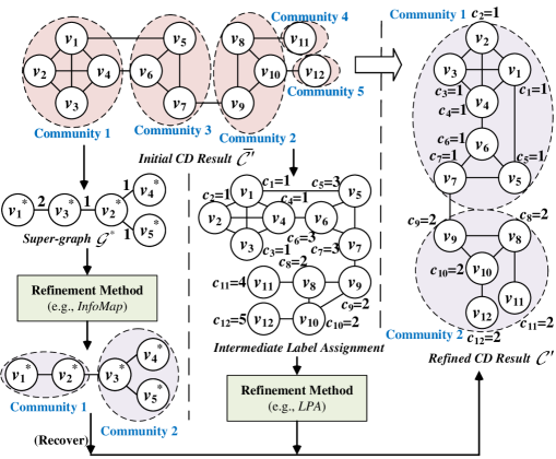
Figure 3. Illustration of the two strategies to construct the initialization of online refinement.

As shown in Fig. 3, we adopt two strategies to construct the initialization. First, a super-graph $\mathcal{G}^{*}$ can be extracted based on $\mathcal{\bar{C}}^{\prime}$, where we merge nodes in each community $\mathcal{\bar{C}}^{\prime}_{r}\in\mathcal{\bar{C}}^{\prime}$ as a super-node (e.g., $v^{*}_{3}$ w.r.t. $\mathcal{\bar{C}}^{\prime}_{3}=\{v_{5},v_{6},v_{7}\}$ in Fig. 3) and set the number of edges between communities as the weight of each super-edge (e.g., $2$ for $(v_{1}^{*},v_{3}^{*})$ in Fig. 3). We then use $\mathcal{G}^{*}$ as the input of an efficient method that can handle weighted graphs (e.g., InfoMap and Locale) to derive a CD result w.r.t. $\mathcal{G}^{*}$, which is further recovered to the result $\mathcal{C}^{\prime}$ w.r.t. $\mathcal{G}^{\prime}$. Second, we also use $\mathcal{\bar{C}}^{\prime}$ as the intermediate label assignment of a method that iteratively updates community labels (e.g., LPA) and refines the label assignment until convergence (e.g., refining $c_{6}$ from $3$ to $1$ in Fig. 3). Compared with running the refinement method on $\mathcal{G}^{\prime}$ from scratch, online refinement may be more efficient, because the constructed initialization reduces the number of nodes to be partitioned and iterations to update community labels. It is also expected that PRoCD can transfer the capability of capturing community structures from the pre-training data to $\{\mathcal{G}^{\prime}\}$.

Input: large real graph $\mathcal{G}^{\prime}$ to be partitioned; saved model parameters $\Theta^{*}$

Output: CD results $\mathcal{C}^{\prime}$ w.r.t. $\mathcal{G}^{\prime}$

1 get input feature ${\bf{X^{\prime}}}$ w.r.t. $\mathcal{G}^{\prime}$ via (3)

2 get a feasible CD result $\mathcal{\bar{C}}^{\prime}$ w.r.t. $\mathcal{G}^{\prime}$ via Algorithm 1

3 construct the initialization for refinement based on $\mathcal{\bar{C}}^{\prime}$

get refined CD result $\mathcal{C}^{\prime}$ via an efficient refinement method

Algorithm 3 Online Generalization & Refinement

Algorithm 3 concludes the aforementioned procedure. The complexity of online generalization (i.e., lines 1-2) is $\mathcal{O}((N+M)d^{2})$, where $N$ and $M$ are the numbers of nodes and edges; $d$ is the embedding dimensionality. The complexity of online refinement (i.e., lines 3-4) depends on the refinement method, which is usually efficient. We leave detailed complexity analysis in Appendix B.

Table 2. Statistics of datasets.

Datasets	$N$	$E$	Min	Max	Avg Deg	Density
Protein (Stark et al., 2006)	81,574	1,779,885	1	4,983	43.6	5e-4
ArXiv (Wang et al., 2020)	169,343	1,157,799	1	13,161	13.7	8e-5
DBLP (Yang and Leskovec, 2012)	317,080	1,049,866	1	343	6.6	2e-5
Amazon (Yang and Leskovec, 2012)	334,863	925,872	1	549	5.5	2e-5
Youtube (Yang and Leskovec, 2012)	1,134,890	2,987,624	1	28,754	5.3	5e-6
RoadCA (Leskovec et al., 2009)	1,957,027	2,760,388	1	12	2.82	1e-6

Table 3. Evaluation results w.r.t. efficiency metric of inference time$\downarrow$ (sec) and quality metric of modularity$\uparrow$.

	Protein			ArXiv			DBLP			Amazon			Youtube			RoadCA
	K	Time$\downarrow$	Mod$\uparrow$	K	Time$\downarrow$	Mod$\uparrow$	K	Time$\downarrow$	Mod$\uparrow$	K	Time$\downarrow$	Mod$\uparrow$	K	Time$\downarrow$	Mod$\uparrow$	K	Time$\downarrow$	Mod$\uparrow$
MC-SBM	170	1143.93	0.1463	303	1014.63	0.5205	430	646.91	0.7620	368	799.05	0.8860	186	6608.67	0.2027	324	8492.20	0.9491
Par-SBM	1494	39.18	0.4721	4936	40.26	0.0529	10854	28.04	0.2797	10813	39.40	0.3094	27948	236.61	0.0901	39987	149.10	0.5970
GMod	69	5840.49	0.6319	1317	6693.91	0.5797	OOT	OOT	OOT	1669	12729.36	0.8703	OOT	OOT	OOT	OOT	OOT	OOT
Louvain	60	46.23	0.6366	155	49.07	0.7059	209	83.50	0.8209	240	48.10	0.9262	6105	173.70	0.7218	376	408.25	0.9923
RaftGP-C	218	69.82	0.6124	213	79.11	0.6147	39	81.99	0.6594	53	87.66	0.7530	1	254.77	0.0000	256	470.05	0.8072
RaftGP-M	185	69.44	0.6199	194	80.10	0.6107	39	83.48	0.6644	54	88.24	0.7561	131	272.82	0.6659	256	469.14	0.8043
LouNE+DBSCAN	32	77.20	0.6362	170	214.55	0.7058	737	109.87	0.8065	252	64.45	0.9255	17908	671.52	0.6228	19081	236.46	0.9531
SktNE+DBSCAN	371	16.18	0.1808	388	542.92	0.3533	15341	45.60	0.5716	13283	49.85	0.7047	17799	485.72	0.1076	59726	1410.91	0.4073
ICD-C+DBSCAN	1277	89.30	0.4961	256	296.02	0.0011	3694	1795.04	0.1047	1865	2027.30	0.0278	OOT	OOT	OOT	OOT	OOT	OOT
ICD-M+DBSCAN	1091	88.47	0.5651	264	294.13	0.0019	3950	984.98	0.1156	2478	872.11	0.0430	OOT	OOT	OOT	OOT	OOT	OOT
LPA	1919	132.32	0.5925	11467	113.30	0.3752	46630	146.22	0.6196	41693	76.49	0.7090	111887	370.15	0.5520	606249	245.54	0.5524
PRoCDw/ LPA	1499	32.07	0.6046	10765	19.93	0.6188	38684	20.10	0.6336	34270	20.40	0.7240	93566	68.72	0.6150	391735	67.74	0.5765
Improve.		+75.8%	+2.1%		+82.4%	+64.9%		+86.3%	+2.3%		+73.3%	+2.1%		+81.4%	+11.4%		+72.4%	+4.4%
GC+LPA	1985	32.52	0.5790	12854	21.57	0.5290	44494	30.04	0.5906	41513	29.40	0.5723	124044	69.17	0.2710	442623	106.89	0.4838
InfoMap	11	26.38	0.1972	69	19.69	0.6332	527	29.11	0.8195	13	28.72	0.8037	956	114.63	0.6959	3	259.44	0.6455
PRoCDw/ IM	18	15.60	0.1996	42	17.08	0.6349	298	17.23	0.8222	417	16.66	0.9222	438	83.01	0.6811	145	79.48	0.9889
Improve.		+40.9%	+1.2%		+13.3%	+0.3%		+40.8%	+0.3%		+42.0%	+14.7%		+27.6%	-2.1%		+69.4%	+53.2%
GC+IM	9	33.84	0.1318	48	24.28	0.4735	305	27.99	0.8086	4	28.01	0.4189	687	104.85	0.6919	3	129.74	0.6561
Locale	51	43.04	0.6409	150	46.66	0.7159	298	40.08	0.8375	392	30.85	0.9343	3441	216.12	0.7353	410	172.48	0.9935
PRoCDw/ Lcl	35	16.93	0.6362	64	31.76	0.7133	147	24.15	0.8376	173	18.94	0.9319	1647	161.24	0.7315	330	90.88	0.9930
Improve.		+60.7%	-0.7%		+31.9%	-0.4%		+39.8%	+0.01%		+38.6%	-0.3%		+25.4%	-0.5%		+47.3%	-0.1%
GC+Lcl	33	44.35	0.6343	150	45.17	0.6988	196	36.87	0.8254	344	30.09	0.9220	3228	194.49	0.7315	327	130.57	0.9928

Table 4. Detailed inference time (sec) of PRoCD.

Datasets	Methods	Feat	FFP	Init	Rfn
Protein	PRoCD w/ LPA	2.84	4.42	6.50	18.31
	PRoCD w/ InfoMap				1.84
	PRoCD w/ Locale				3.17
ArXiv	PRoCD w/ LPA	1.49	0.99	4.50	12.96
	PRoCD w/ InfoMap				10.11
	PRoCD w/ Locale				24.79
DBLP	PRoCD w/ LPA	1.97	1.28	4.19	12.66
	PRoCD w/ InfoMap				9.79
	PRoCD w/ Locale				16.71
Amazon	PRoCD w/ LPA	2.08	1.99	3.81	12.51
	PRoCD w/ InfoMap				8.78
	PRoCD w/ Locale				11.06
Youtube	PRoCD w/ LPA	5.81	2.75	15.13	45.02
	PRoCD w/ InfoMap				59.32
	PRoCD w/ Locale				137.54
RoadCA	PRoCD w/ LPA	8.10	2.34	13.14	44.16
	PRoCD w/ InfoMap				55.90
	PRoCD w/ Locale				67.31

Table 5. Detailed inference time (sec) of graph GC baselines.

Datasets	Methods	GC	Rfn
Protein	GC+LPA	15.20	17.32
	GC+InfoMap		18.64
	GC+Locale		29.15
ArXiv	GC+LPA	10.20	11.37
	GC+InfoMap		14.08
	GC+Locale		34.97
DBLP	GC+LPA	17.84	12.20
	GC+InfoMap		10.15
	GC+Locale		19.03
Amazon	GC+LPA	17.19	12.21
	GC+InfoMap		10.82
	GC+Locale		12.90
Youtube	GC+LPA	31.84	37.32
	GC+InfoMap		73.01
	GC+Locale		162.65
RoadCA	GC+LPA	71.33	35.56
	GC+InfoMap		58.41
	GC+Locale		59.24

Table 6. Detailed inference time (s) of embedding baselines.

Datasets	Methods	Emb	Clus
Protein	LouvainNE+DBSCAN	4.13	73.07
	SketchNE+DBSCAN	4.30	11.88
	ICD-C+DBSCAN	6.99	82.31
	ICD-M+DBSCAN	12.49	75.97
ArXiv	LouvainNE+DBSCAN	6.86	207.41
	SketchNE+DBSCAN	5.79	537.12
	ICD-C+DBSCAN	21.59	274.43
	ICD-M+DBSCAN	19.57	274.55
DBLP	LouvainNE+DBSCAN	10.52	99.35
	SketchNE+DBSCAN	7.71	37.90
	ICD-C+DBSCAN	5.66	1789.38
	ICD-M+DBSCAN	11.53	973.45
Amazon	LouvainNE+DBSCAN	10.79	53.67
	SketchNE+DBSCAN	8.05	41.79
	ICD-C+DBSCAN	16.26	2011.04
	ICD-M+DBSCAN	23.22	848.89
Youtube	LouvainNE+DBSCAN	34.98	635.55
	SketchNE+DBSCAN	19.40	466.32
	ICD-C+DBSCAN	10.43	OOT
	ICD-M+DBSCAN	7.66	OOT
RoadCA	LouvainNE+DBSCAN	56.30	180.15
	SketchNE+DBSCAN	25.11	1385.80
	ICD-C+DBSCAN	14.49	OOT
	ICD-M+DBSCAN	12.90	OOT

5. Experiments

In this section, we elaborate on our experiments, including the experiment setup, evaluation results, ablation study, and parameter analysis. We will make the datasets and demo code public at https://github.com/KuroginQin/PRoCD.

5.1. Experiment Setup

Datasets. We evaluated the inference efficiency and quality of our PRoCD method on $6$ public datasets with statistics depicted in Table 2, where $N$ and $M$ are the numbers of nodes and edges. Note that these datasets do not provide ground-truth about the community assignment and the number of communities $K$. Some more details regarding the datasets can be found in Appendix C.1.

Baselines. We compared PRoCD over $11$ baselines.

(i) MC-SBM (Peixoto, 2014), (ii) Par-SBM (Peng et al., 2015), (iii) GMod (Clauset et al., 2004), (iv) LPA (Raghavan et al., 2007), (v) InfoMap (Rosvall and Bergstrom, 2008), (vi) Louvain (Blondel et al., 2008), and (vii) Locale (Wang and Kolter, 2020), and (viii) RaftGP (Gao et al., 2023) are efficient end-to-end methods that can tackle $K$-agnostic CD. Note that some other approaches whose designs rely on a pre-set $K$ (e.g., FastCom (Clauset et al., 2004), GraClus (Dhillon et al., 2007), ClusterNet (Wilder et al., 2019), LGNN (Chen et al., 2019), and DMoN (Tsitsulin et al., 2023)) could not be included in our experiments.

In addition, we extended (ix) LouvainNE (Bhowmick et al., 2020), (x) SketchNE (Xie et al., 2023), and (xi) ICD (Qin et al., 2023b), which are state-of-the-art efficient graph embedding methods, to $K$-agnostic CD by combining the derived embeddings with DBSCAN (Schubert et al., 2017), an efficient clustering algorithm that does not require $K$. In particular, LouvainNE and ICD are claimed to be community-preserving methods. RaftGP-C, RaftGP-M, ICD-C, and ICD-M denote different variants of RaftGP and ICD.

As a demonstration, we adopted LPA, InfoMap, and Locale (an advanced extension of Louvain) for the online refinement of PRoCD, forming three variants of our method. In Fig. 3, the first strategy of constructing the refinement initialization has a motivation similar to graph coarsening (GC) techniques (Chen et al., 2022), which merge a large graph $\mathcal{G}^{\prime}$ into a super-graph $\mathcal{G}^{*}$ (i.e., reducing the number of nodes to be partitioned) via a heuristic strategy. Whereas, PRoCD constructs $\mathcal{G}^{*}$ based on the output of a pre-trained model. To highlight the superiority of offline pre-training and inductive inference beyond GC, we introduced another baseline that provides the initialization (with the same number of super-nodes as PRoCD) for online refinement using the efficient GC strategy proposed in (Liang et al., 2021).

ICD is an inductive baseline with a paradigm similar to PRoCD, including offline (pre-)training on historical graphs and online generalization to new graphs. However, there is no online refinement in ICD. We conducted the offline pre-training of ICD and PRoCD on the generated synthetic graphs as described in Section 4.2.1 and generalized them to each dataset for online inference. For the rest baselines, we had to run them from scratch on each dataset.

Evaluation Criteria. Following the evaluation protocol described in Section 3, we adopted modularity and inference time (sec) as the quality and efficiency metrics. Moreover, we define that a method encounters the out-of-time (OOT) exception if it fails to derive a feasible CD result within $2\times 10^{4}$ seconds.

Due to space limits, we elaborate on other details of experiment setup (e.g., parameter settings) in Appendix C.

5.2. Quantitative Evaluation & Discussions

The average evaluation results are reported in Table 3. Besides the total inference time, we also report the time w.r.t. each inference phase of PRoCD in Table 4, where ‘Feat’, ‘FFP’, ‘Init’, and ‘Rfn’ denote the time of (i) feature extraction, (ii) one FFP, (iii) initial result derivation, and (iv) online refinement. Analysis about the inference time of GC and embedding baselines is given in Tables 5 and 6, where ‘GC’, ‘Rfn’, ‘Emb’, and ‘Clus’ denote the time of (i) graph coarsening, (ii) online refinement, (iii) embedding derivation, and (iv) downstream clustering (i.e., via DBSCAN).

In Table 3, three variants of PRoCD achieve significant improvement of efficiency w.r.t. the refinement methods while the quality degradation is less than $2\%$. In some cases, PRoCD can even obtain improvement for both aspects. Compared with all the baselines, PRoCD can ensure the best efficiency on all the datasets and is in groups with the best quality. In summary, we believe that the proposed method provides a possible way to obtain a better trade-off between the quality and efficiency in CD.

In most cases, PRoCD outperforms GC baselines in both aspects, which validates the superiority of offline pre-training and inductive inference beyond heuristic GC. The extensions of some embedding baselines (e.g., SketchNE and ICD combined with DBSCAN) suffer from low quality and efficiency compared with other end-to-end approaches (e.g., Louvain and Locale). It implies that the task-specific module (e.g., binary node pair classifier in PRoCD) is essential for the embedding framework to ensure the quality and efficiency in $K$-agnostic CD, which is seldom considered in related studies.

According to Table 4, online refinement is the major bottleneck in the inference of PRoCD, with the runtime depending on concrete refinement methods. Compared with running a refinement method from scratch, online refinement has much lower runtime. It validates our motivation that constructing the initialization (as described in Fig. 3) can reduce the number of nodes to be partitioned and iterations to update label assignments for refinement methods. To construct the initialization of online refinement, GC is not as efficient as the online generalization of PRoCD (i.e., feature extraction, one FFP, and initial result derivation) according to Table 5. In Table 6, the downstream clustering (i.e., DBSCAN to derive a feasible result for $K$-agnostic CD) is time-consuming, which results in low efficiency of the extended embedding baselines, although their embedding derivation phases are efficient.

Table 7. Ablation studies on DBLP and Amazon in terms of modularity$\uparrow$ and inference time$\downarrow$ (sec).

	DBLP			Amazon
	K	Mod$\uparrow$	Time$\downarrow$	K	Mod$\uparrow$	Time$\downarrow$
(i)w/o Rfn	106553	0.4394	7.44	112408	0.5620	7.88
PRoCD w/ LPA	38684	0.6336	20.10	34270	0.7240	20.40
(ii)w/o Ptn	1	0.0000	9.75	1	0.0000	8.81
(iii)w/o Feat (3)	537	0.0625	18.01	1	0.0000	6.29
(iv)w/o EmbEnc (4)	58401	0.5406	18.26	53127	0.5090	17.08
(v)w/o BinClf (6)	48	0.0009	6.43	23	0.0008	6.31
(vi)w/o $\mathcal{L}_{\rm{BCE}}$ (8)	22496	0.5657	17.84	16378	0.6580	20.19
(vii) w/o $\mathcal{L}_{\rm{MOD}}$ (7)	39792	0.6261	20.12	34853	0.7188	19.31
PRoCD w/ IM	298	0.8222	17.23	417	0.9222	16.66
(ii)w/o Ptn	1	0.0000	9.75	1	0.0000	8.81
(iii)w/o Feat (3)	2	0.0001	5.67	1	0.0000	5.13
(iv)w/o EmbEnc (4)	516	0.8182	26.55	6	0.3869	39.27
(v)w/o BinClf (6)	48	0.0009	5.88	23	0.0008	5.68
(vi)w/o $\mathcal{L}_{\rm{BCE}}$ (8)	156	0.2895	12.93	356	0.4872	9.91
(vii)w/o $\mathcal{L}_{\rm{MOD}}$ (7)	306	0.8200	19.22	2	0.2638	22.06
PRoCD w/ Lcl	147	0.8376	24.15	173	0.9319	18.94
(ii)w/o Ptn	1	0.0000	9.75	1	0.0000	8.81
(iii)w/o Feat (3)	551	0.0647	5.66	1	0.0000	5.15
(iv)w/o EmbEnc (4)	216	0.8368	42.20	307	0.9228	35.97
(v)w/o BinClf (6)	48	0.0009	6.66	23	0.0008	6.43
(vi)w/o $\mathcal{L}_{\rm{BCE}}$ (8)	305	0.7460	18.04	776	0.7448	19.23
(vii)w/o $\mathcal{L}_{\rm{MOD}}$ (7)	143	0.8365	25.97	210	0.9228	17.76

5.3. Ablation Study

For our PRoCD method, we verified the effectiveness of (i) online refinement, (ii) offline pre-training, (iii) feature extraction module in (3), (iv) embedding encoder in (4), (v) binary node pair classifier in (6), (vi) cross-entropy objective $\mathcal{L}_{\rm{BCE}}$, and (vii) modularity maximization objective $\mathcal{L}_{\rm{MOD}}$ by removing corresponding components from the original model. In case (iii), we let ${\bf{X}}$ be the one-hot encodings of node degree, which is a standard feature extraction strategy for GNNs when attributes are unavailable. We directly used ${\bf{X}}$ as the derived embeddings in case (iv), while we adopted the naive binary classifier (5) to replace our design (6) in case (v). The average ablation study results on DBLP and Amazon are reported in Table 7, where there are quality declines in all the cases. In some extreme cases (e.g., the one without pre-training), the model mistakenly partitions all the nodes into one community, resulting in a modularity value of $0.0000$. In summary, all the considered procedures and components are essential to ensure the quality of PRoCD.

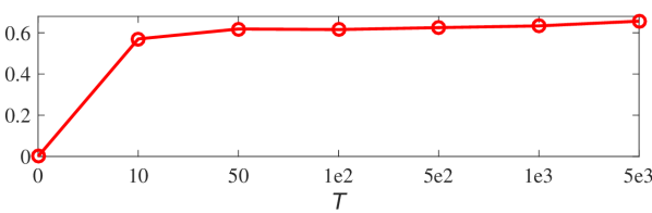
(a) DBLP, w/ LPA

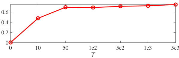
(b) Amazon, w/ LPA

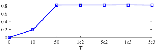
(c) DBLP, w/ InfoMap

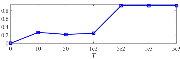
(d) Amazon, w/ InfoMap

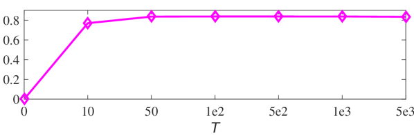
(e) DBLP, w/ Locale

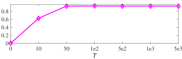
(f) Amazon, w/ Locale

Figure 4. Ablation study w.r.t. the number of pre-training graphs $T$ on DBLP and Amazon in terms of modularity$\uparrow$.

To further verify the significance of offline pre-training in our PRoCD method, we conducted additional ablation study by setting the number of pre-training graphs $T\in\{0,10,50,1e2,5e2,1e3,5e3\}$. The corresponding results on DBLP and Amazon in terms of modularity are reported in Fig. 4. Compared with our standard setting (i.e., $T=1e3$), there are significant quality declines for all the variants of PRoCD when there are too few pre-training graphs (e.g., $T<50$). It implies that the offline pre-training (with enough synthetic graphs) is essential to ensure the high inference quality of PRoCD.

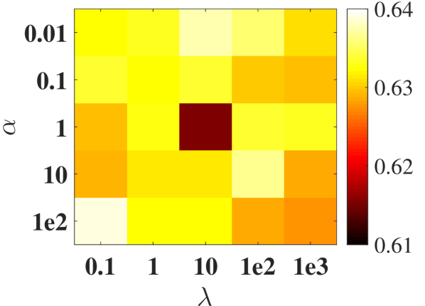
(a) DBLP, w/ LPA

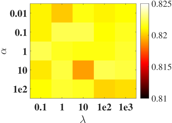
(b) DBLP, w/ InfoMap

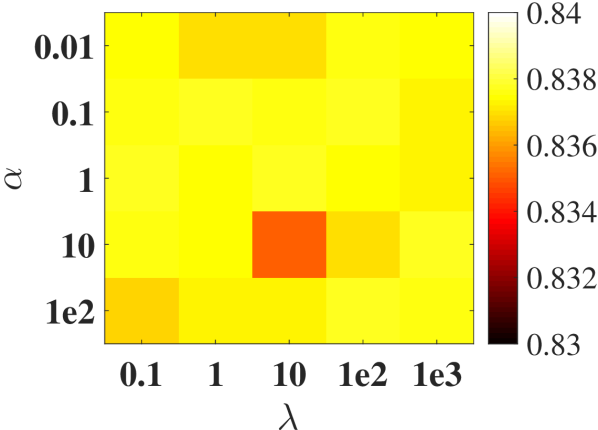
(c) DBLP, w/ Locale

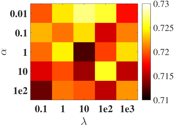
(d) Amazon, w/ LPA

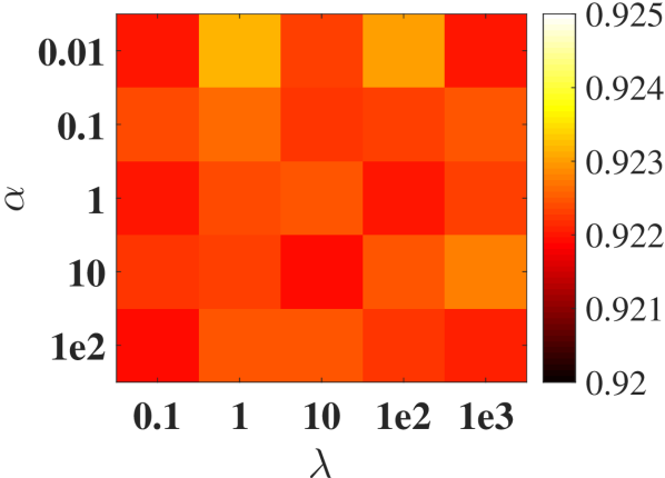
(e) Amazon, w/ InfoMap

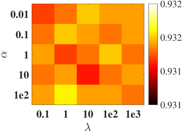
(f) Amazon, w/ Locale

Figure 5. Parameter analysis w.r.t. $\alpha$ and $\lambda$ on DBLP and Amazon in terms of modularity$\uparrow$.

5.4. Parameter Analysis

We also tested the effects of $\{\alpha,\lambda\}$ in the pre-training objective (9) by adjusting $\alpha\in\{0.01,0.1,1,10,100\}$ and $\lambda\in\{0.1,1,10,100,1000\}$. The example parameter analysis results on DBLP and Amazon in terms of modularity are shown in Fig. 5, where different settings of $\{\alpha,\lambda\}$ would not significantly affect the quality of PRoCD. The influence of $\{\alpha,\lambda\}$ may also differ from refinement methods. For instance, LPA is more sensitive to the parameter setting, compared with InfoMap and Locale.

Due to space limit, we leave further parameter analysis about the number of sampled node pair $n_{S}$ (see Algorithm 1) in Appendix D.

6. Conclusion

In this paper, we explored the potential of DGL to achieve a better trade-off between the quality and efficiency of $K$-agnostic CD. By reformulating this task as the binary node pair classification, a simple yet effective PRoCD method was proposed. It follows a novel pre-training & refinement paradigm, including the (i) offline pre-training on small synthetic graphs with various topology properties and high-quality ground-truth as well as the (ii) online generalization to and (iii) refinement on large real graphs without additional model optimization. Extensive experiments demonstrate that PRoCD, combined with different refinement methods, can achieve higher inference efficiency without significant quality degradation on public real graphs with various scales. Some possible future research directions are summarized in Appendix E.

Appendix A Generation of Pre-training Data

Table 8. Parameter settings of the synthetic graph generator.

$T$	$N$	$K$	${\deg}_{\min}$	${\deg}_{\max}$	$\gamma$	$\mu$	$\rho$
1e3	I(2e3, 5e3)	I(2, 1e3)	min{5, $\left\lceil{N/(4K)}\right\rceil$ }	min{5e2, $\left\lceil{N/K}\right\rceil$}	F(2, 3.5)	F(2.5, 5)	F(1, 3)

Table 9. Statistics of the generated synthetic pre-training graphs.

Min	Max	Avg $N$	Min	Max	Avg $E$	Min	Max	Avg $K$	Avg ${\deg}_{\min}$	Avg ${\deg}_{\max}$	Min	Max	Avg Density
2,000	5,000	3,495.1	2,049	66,355	12,115.3	2	968	485.3	1.3	20.8	4e-4	1e-2	2e-3

Our settings of the DC-SBM generator are summarized in Table 8, where ‘I($a$, $b$)’ and ‘F($a$, $b$)’ denote an integer and a float uniformly sampled from the range $[a,b]$; $T$ is the number of synthetic graphs; $N$ and $K$ are the numbers of nodes and communities in each graph; ${\deg}_{\min}$ and ${\deg}_{\max}$ are the minimum and maximum node degrees of a graph; $\gamma$ is a parameter to control the power-law distributions of node degrees with ${\deg}(v_{i})\sim\{{k^{\gamma}}/\sum\nolimits_{l={{\deg}_{\min}}}^{{{\deg}_{\max}}}{{l^{\gamma}}}\}$ (${\deg}_{\min}\leq k\leq{\deg}_{\max}$); $\mu$ is a ratio between the number of within-community and between-community edges; $\rho$ is a parameter to control the heterogeneity of community size, with the size of each community following ${\mathop{\rm Dirichlet}\nolimits}(10/\rho)$.

Input: number of nodes $N_{t}$; number of communities $K_{t}$; range [${\deg}_{\min},{\deg}_{\max}$] for node degrees; $\gamma$ for degree distribution; $\mu$ for numbers of within-community edges and between-community edges; $\rho$ for community size distribution

Output: a synthetic graph $\mathcal{G}_{t}=(\mathcal{V}_{t},\mathcal{E}_{t})$

1 generate node set $\mathcal{V}_{t}=\{v_{1},\cdots,v_{N_{t}}\}$

2 for $r$ from $1$ to $K_{t}$ do

3       get size of the $r$-th community $|\mathcal{C}_{r}^{(t)}|\sim{\mathop{\rm Dirichlet}\nolimits}(10/\rho)$

4       initialize $\mathcal{C}_{r}^{(t)}$’s degree sum $\varphi_{r}\leftarrow 0$

5initialize total degree sum ${\bar{\varphi}}\leftarrow 0$

6 for each node $v_{i}\in\mathcal{V}_{t}$ do

7       get $v_{i}$’s community label $c_{i}\sim{\mathop{\rm Multi}\nolimits}(|\mathcal{C}_{1}^{(t)}|,\cdots,|\mathcal{C}_{{K_{t}}}^{(t)}|)$

8       add $v_{i}$ into corresponding community $\mathcal{C}_{c_{i}}$

9       get $v_{i}$’s degree ${\deg}(v_{i})\sim\{{k^{\gamma}}/\sum\limits_{l={{\deg}_{\min}}}^{{{\deg}_{\max}}}{{l^{\gamma}}}|{{\deg}_{\min}}\leq k\leq{{\deg}_{\max}}\}$

10       update degree sum $\varphi_{c_{i}}\leftarrow\varphi_{c_{i}}+{\deg}(v_{i})$

11       update total degree sum ${\bar{\varphi}}\leftarrow{\bar{\varphi}}+{\deg}(v_{i})$

12for each node $v_{i}\in\mathcal{V}_{t}$ do

13       get $v_{i}$’s degree correction value ${\bf{\theta}}_{i}\leftarrow{\deg}(v_{i})/\varphi_{c_{i}}$

14      

15for $r$ from $1$ to $K_{t}$ do

16       for $t$ from $r$ to $K_{t}$ do

17             if $r=t$ then

18                   ${\bf{\Omega_{rr}}}\leftarrow\frac{\mu}{{1+\mu}}\cdot{\varphi_{r}}$

19            else

20                   ${\bf{\Omega_{rt}}}\leftarrow\frac{1}{{1+\mu}}\cdot\frac{{{\varphi_{r}}{\varphi_{t}}}}{{\bar{\varphi}}}$

21            

22      

23for $i$ from $2$ to $N_{t}$ do

24       for $j$ from $1$ to $i$ do

25             generate an edge $(v_{i},v_{j})$ for $\mathcal{E}_{t}$ via ${\mathop{\rm Poisson}\nolimits}({{\bf{\theta}}_{i}}{{\bf{\theta}}_{j}}{{\bf{\Omega}}_{{c_{i}}{c_{j}}}})$

26      

Algorithm 4 Generating a Synthetic Graph via DC-SBM

For each synthetic graph $\mathcal{G}_{t}$, suppose there are $N_{t}$ nodes partitioned into $K_{t}$ communities, with $N_{t}$ and $K_{t}$ sampled from the corresponding distributions in Table 8. Let $\mathcal{C}^{(t)}=\{\mathcal{C}_{1}^{(t)},\cdots,\mathcal{C}_{K_{t}}^{(t)}\}$ denote the community ground-truth of $\mathcal{G}_{t}$. We also sample $(\gamma,\mu,\rho)$ from corresponding distributions in Table 8, which define the topology properties of $\mathcal{G}_{t}$. Algorithm 4 summarizes the procedure of generating a graph $\mathcal{G}_{t}$ via DC-SBM, based on the parameter settings of $\{N_{t},K_{t},{\deg}_{\min},{\deg}_{\max},\gamma,\mu,\rho\}$. Concretely, DC-SBM generates an edge $(v_{i},v_{j})$ in each graph $\mathcal{G}_{t}$ via ${\bf{A}}^{(t)}_{ij}\sim{\mathop{\rm Poisson}\nolimits}({\bf{\theta}}_{i}{\bf{\theta}}_{j}{\bf{\Omega}}_{{c_{i}}{c_{j}}})$, where $c_{i}$ is the community label of node $v_{i}$; ${\bf{\theta}}\in\mathbb{R}_{+}^{N_{t}}$ and ${\bf{\Omega}}\in\mathbb{R}_{+}^{K_{t}\times K_{t}}$ are the degree correction vector and block interaction matrix (Karrer and Newman, 2011) determined by $\{\gamma,\mu,\rho\}$; ${\bf{\theta}}_{i}{\bf{\theta}}_{j}{\bf{\Omega}}_{{c_{i}}{c_{j}}}$ represents the expected number of edges between $v_{i}$ and $v_{j}$.

Statistics of the generated synthetic graphs (used for offline pre-training in our experiments) are reported in Table 9.

Appendix B Detailed Complexity Analysis

For each graph $\mathcal{G}^{\prime}$, let $N$, $M$, and $d$ be the number of nodes, number of edges, and embedding dimensionality, respectively. By using the efficient sparse-dense matrix multiplication, the complexity of the feature extraction defined in (3) is $\mathcal{O}(Md+Nd^{2})$. Similarly, the complexity of one FFP of the embedding encoder described by (4) is no more than $\mathcal{O}(Md+Nd^{2})$.

To derive a feasible CD result via Algorithm 1, the complexities of constructing the node pair set $\mathcal{P}$, one FFP of the binary classifier to derive auxiliary graph $\mathcal{\tilde{G}}$, and extracting connected components via DFS/BFS are $\mathcal{O}(M+n_{S})$, $\mathcal{O}((M+n_{S})d^{2})$, and $\mathcal{O}(N+{\tilde{M}})$, where $n_{S}$ is the number of randomly sampled node pairs; ${\tilde{M}}:=|\mathcal{\tilde{E}}|$ is the number of edges in the auxiliary graph $\mathcal{\tilde{G}}$.

In summary, the complexity of online generalization is $\mathcal{O}((Md+Nd^{2})+(Md+Nd^{2})+(M+n_{S})+(M+n_{S})d^{2}+(N+{\tilde{M}}))=\mathcal{O}((N+M)d^{2})$, where we assume that $\tilde{M}\approx M$, and $n_{S}\ll M$.

Appendix C Detailed Experiment Setup

C.1. Datasets

In the six real datasets (see Table 2), Protein (Stark et al., 2006) was collected based on the protein-protein interactions in the BioGRID repository. ArXiv (Wang et al., 2020) and DBLP (Yang and Leskovec, 2012) are public paper citation and collaboration graphs extracted from ArXiv and DBLP, respectively. Amazon (Yang and Leskovec, 2012) was collected by crawling the product co-purchasing relations from Amazon, while Youtube (Yang and Leskovec, 2012) was constructed based on the friendship relations of Youtube. RoadCA (Leskovec et al., 2009) describes a road network in California. To pre-process Protein, we abstracted each protein as a unique node and constructed graph topology based on corresponding protein-protein interactions. Since there are multiple connected components in the extracted graph, we extracted the largest component for evaluation. Moreover, we used original formats of the remaining datasets provided by their sources.

C.2. Environments & Implementation Details

All the experiments were conducted on a server with one AMD EPYC 7742 64-Core CPU, $512$GB main memory, and one $80$GB memory GPU. We used Python 3.7 to implement PRoCD, where the feature extraction module (3), embedding encoder (4), and binary node pair classifier (6) were implemented via PyTorch 1.10.0. Hence, the feature extraction and FFP of PRoCD can be speeded up via the GPU. The efficient function ‘scipy.sparse.csgraph.connected_components’ was used to extract connected components in Algorithm 1 to derive a feasible CD result. For all the baselines, we adopted their official implementations and tuned parameters to report the best quality. To ensure the fairness of comparison, the embedding dimensionality of all the embedding-based methods (i.e., LouvainNE, SketchNE, RaftGP, ICD, and PRoCD) was set to be the same (i.e., $64$).

Table 10. Detailed parameter settings of PRoCD.

Datasets	Parameter Settings			Layer Configurations
	($\alpha$, $\lambda$)	($n_{P}$, $\eta$)	$n_{S}$	$d$	$L_{\rm{Feat}}$	$L_{\rm{GNN}}$	$L_{\rm{BC}}$
Protein	(0.1, 1)	(20, 1e-4)	1e3	64	2	4	2
ArXiv	(1, 100)	(100, 1e-4)	1e4			2	6
DBLP	(0.1, 10)	(100, 1e-4)	1e4			4	2
Amazon	(0.1, 10)	(100, 1e-4)	2e4			4	2
Youtube	(1e2, 1e2)	(89, 1e-4)	1e4			4	2
RoadCA	(1e2, 10)	(11, 1e-4)	1e4			2	2

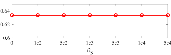
(a) DBLP, w/ LPA

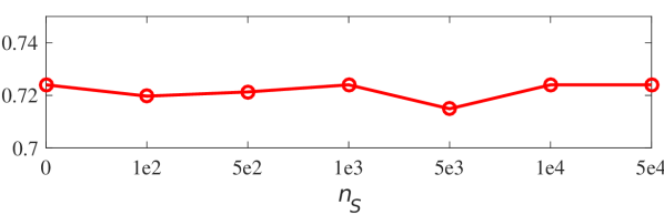
(b) Amazon, w/ LPA

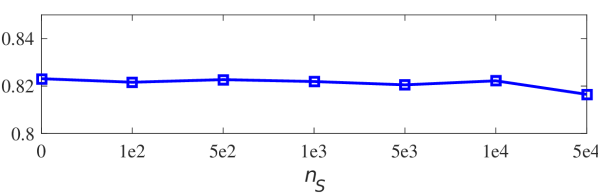
(c) DBLP, w/ InfoMap

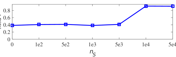
(d) Amazon, w/ InfoMap

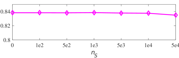
(e) DBLP, w/ Locale

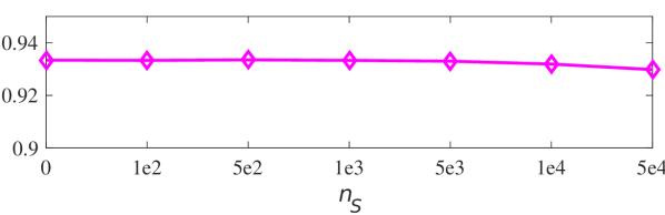
(f) Amazon, w/ Locale

Figure 6. Parameter analysis w.r.t. the number of sampled node pairs $n_{S}$ on DBLP and Amazon in terms of modularity$\uparrow$.

C.3. Parameter Settings & Layer Configurations

The recommended parameter settings and layer configurations of PRoCD are depicted in Table 10, where $\alpha$ and $\lambda$ are hyper-parameters in the pre-training objective (9); $n_{P}$ and $\eta$ are the number of epochs and learning rate of pre-training in Algorithm 2; $n_{S}$ is the number of randomly sampled node pairs in Algorithm 1 for inference; $d$ is the embedding dimensionality; $L_{\rm{Feat}}$, $L_{\rm{GNN}}$, and $L_{\rm{BC}}$ are the numbers of MLP layers in (3), GNN layers in (4), and MLP layers in (6). Given an MLP, let ${\bf{u}}^{[s-1]}$ and ${\bf{u}}^{[s]}$ be the input and output of the $s$-th perceptron layer. The MLP in the feature extraction module (3) is defined as

(10) $${{\bf{u}}^{[s]}}=\tanh({{\bf{u}}^{[s-1]}}{{\bf{W}}^{[s]}}+{{\bf{b}}^{[s]}}),$$

with $\{{\bf{W}}^{[s]}\in\mathbb{R}^{d\times d},{\bf{b}}^{[s]}\in\mathbb{R}^{d}\}$ as trainable parameters. For the MLP $h_{s}(\cdot)$ (or $h_{d}(\cdot)$) in the binary classifier (6), suppose there are $L$ layers. The $s$-th layer ($s<L$) and the last layer of $h_{s}(\cdot)$ (or $h_{d}(\cdot)$) are defined as

(11) $${{\bf{u}}^{[s]}}=\tanh({{\bf{u}}^{[s-1]}}{{\bf{W}}^{[s]}}+{{\bf{b}}^{[s]}})+{{\bf{u}}^{[s-1]}},$$

(12) $${{\bf{u}}^{[L]}}={\mathop{\rm ReLU}\nolimits}({{\bf{u}}^{[L-1]}}{{\bf{W}}^{[L]}}+{{\bf{b}}^{[L]}}),$$

where there is a skip connection in each perceptron layer except the last layer.

Appendix D Further Experiment Results

We also conducted parameter analysis for the number of sampled node pairs (in Algorithm 1) for inference, where we set $n_{S}\in\{0,1e2,5e2,1e3,5e3,1e4,5e4\}$. Results on DBLP and Amazon in terms of modularity are shown in Fig. 6. In most cases except the variant with InfoMap on Amazon, our PRoCD method is not sensitive to the setting of $n_{S}$. To ensure the inference quality of the exception case, one needs a large setting of $n_{S}$ (e.g., $n_{S}\geq 1e4$).

Appendix E Future Directions

Some possible future directions are summarized as follows.

Theoretical Analysis. This study empirically verified the potential of PRoCD to achieve a better trade-off between the quality and efficiency of $K$-agnostic. However, most existing graph pre-training techniques lack theoretical guarantee for their transfer ability w.r.t. different pre-training data and downstream tasks. We plan to theoretically analyze the transfer ability of PRoCD from small synthetic pre-training graphs to large real graphs, following previous analysis on random graph models (e.g., SBM (Qin and Rohe, 2013; Jin et al., 2021)).

Extension to Dynamic Graphs. In this study, we considered $K$-agnostic CD on static graphs. CD on dynamic graphs (Rossetti and Cazabet, 2018) is a more challenging setting, involving the variation of nodes, edges, and community membership over time. Usually, one can formulate a dynamic graph as a sequence of static snapshots with similar underlying properties (Lei et al., 2019; Qin and Yeung, 2023; Qin et al., 2023a). PRoCD can be easily extended to handle dynamic CD by directly generalizing the pre-trained model to each snapshot for fast online inference, without any retraining. Further validation of this extension is also our next focus.

Integration of Graph Attributes. As stated in Section 3, we considered CD without available graph attributes. A series of previous studies (Newman and Clauset, 2016; Qin et al., 2018; Chunaev et al., 2020; Qin and Lei, 2021; Zhao et al., 2022) have demonstrated the complicated correlations between graph topology and attributes, which are inherently heterogeneous information sources, for CD. On the one hand, the integration of attributes may provide complementary characteristics for better CD quality. On the other hand, it may also incorporate noise or inconsistent features that lead to unexpected quality decline compared with those only considering one source. In our future work, we will explore the adaptive integration of attributes for PRoCD. Concretely, when attributes match well with topology, we expect that PRoCD can fully utilize the complementary information of attributes to improve CD quality. When the two sources mismatch with one another, we try to adaptively control the contribution of attributes to avoid quality decline.

References

- (1)
- Arriaga and Vempala (2006) Rosa I Arriaga and Santosh Vempala. 2006. An algorithmic theory of learning: Robust concepts and random projection. Machine Learning 63 (2006), 161–182.
- Bhowmick et al. (2020) Ayan Kumar Bhowmick, Koushik Meneni, Maximilien Danisch, Jean-Loup Guillaume, and Bivas Mitra. 2020. Louvainne: Hierarchical louvain method for high quality and scalable network embedding. In WSDM. 43–51.
- Blondel et al. (2008) Vincent D Blondel, Jean-Loup Guillaume, Renaud Lambiotte, and Etienne Lefebvre. 2008. Fast unfolding of communities in large networks. Journal of Statistical Mechanics: Theory & Experiment 2008, 10 (2008), P10008.
- Cao et al. (2023) Yuxuan Cao, Jiarong Xu, Carl J. Yang, Jiaan Wang, Yunchao Zhang, Chunping Wang, Lei Chen, and Yang Yang. 2023. When to Pre-Train Graph Neural Networks? From Data Generation Perspective!. In SIGKDD. 142–153.
- Chen et al. (2022) Jie Chen, Yousef Saad, and Zechen Zhang. 2022. Graph coarsening: from scientific computing to machine learning. SeMA Journal (2022), 1–37.
- Chen et al. (2019) Zhengdao Chen, Joan Bruna, and Lisha Li. 2019. Supervised community detection with line graph neural networks. In ICLR.
- Chunaev et al. (2020) Petr Chunaev, Timofey Gradov, and Klavdiya Bochenina. 2020. Community detection in node-attributed social networks: How structure-attributes correlation affects clustering quality. Procedia Computer Science 178 (2020), 355–364.
- Clauset et al. (2004) Aaron Clauset, Mark EJ Newman, and Cristopher Moore. 2004. Finding community structure in very large networks. Physical Review E 70, 6 (2004), 066111.
- Dai and Bai (2017) Lin Dai and Bo Bai. 2017. Optimal decomposition for large-scale infrastructure-based wireless networks. TWC 16, 8 (2017), 4956–4969.
- Dhillon et al. (2007) Inderjit S Dhillon, Yuqiang Guan, and Brian Kulis. 2007. Weighted graph cuts without eigenvectors a multilevel approach. TPAMI 29, 11 (2007), 1944–1957.
- Fortunato (2010) Santo Fortunato. 2010. Community detection in graphs. Physics Reports 486, 3-5 (2010), 75–174.
- Fortunato and Newman (2022) Santo Fortunato and Mark EJ Newman. 2022. 20 years of network community detection. Nature Physics 18, 8 (2022), 848–850.
- Gao et al. (2023) Yu Gao, Meng Qin, Yibin Ding, Li Zeng, Chaorui Zhang, Weixi Zhang, Wei Han, Rongqian Zhao, and Bo Bai. 2023. RaftGP: Random Fast Graph Partitioning. In HPEC. 1–7.
- Jin et al. (2021) Jiashun Jin, Zheng Tracy Ke, and Shengming Luo. 2021. Improvements on score, especially for weak signals. Sankhya A (2021), 1–36.
- Karrer and Newman (2011) Brian Karrer and Mark EJ Newman. 2011. Stochastic blockmodels and community structure in networks. Physical Review E 83, 1 (2011), 016107.
- Kipf and Welling (2016) Thomas N Kipf and Max Welling. 2016. Semi-supervised classification with graph convolutional networks. In ICLR.
- Lei et al. (2019) Kai Lei, Meng Qin, Bo Bai, Gong Zhang, and Min Yang. 2019. GCN-GAN: A non-linear temporal link prediction model for weighted dynamic networks. In InfoCom. 388–396.
- Leskovec et al. (2009) Jure Leskovec, Kevin J Lang, Anirban Dasgupta, and Michael W Mahoney. 2009. Community structure in large networks: Natural cluster sizes and the absence of large well-defined clusters. Internet Mathematics 6, 1 (2009), 29–123.
- Liang et al. (2021) Jiongqian Liang, Saket Gurukar, and Srinivasan Parthasarathy. 2021. Mile: A multi-level framework for scalable graph embedding. In AAAI Conference on Web & Social Media, Vol. 15. 361–372.
- Liu et al. (2022) Yue Liu, Wenxuan Tu, Sihang Zhou, Xinwang Liu, Linxuan Song, Xihong Yang, and En Zhu. 2022. Deep graph clustering via dual correlation reduction. In AAAI, Vol. 36. 7603–7611.
- Liu et al. (2023) Zemin Liu, Xingtong Yu, Yuan Fang, and Xinming Zhang. 2023. Graphprompt: Unifying pre-training and downstream tasks for graph neural networks. In Web Conference. 417–428.
- Lu et al. (2021) Yuanfu Lu, Xunqiang Jiang, Yuan Fang, and Chuan Shi. 2021. Learning to pre-train graph neural networks. In AAAI, Vol. 35. 4276–4284.
- Nazi et al. (2019) Azade Nazi, Will Hang, Anna Goldie, Sujith Ravi, and Azalia Mirhoseini. 2019. Gap: Generalizable approximate graph partitioning framework. arXiv:1903.00614 (2019).
- Newman (2006) Mark EJ Newman. 2006. Modularity and Community Structure in Networks. PNAS 103, 23 (2006), 8577–8582.
- Newman and Clauset (2016) Mark EJ Newman and Aaron Clauset. 2016. Structure and inference in annotated networks. NC 7, 1 (2016), 11863.
- Peixoto (2014) Tiago P Peixoto. 2014. Efficient Monte Carlo and greedy heuristic for the inference of stochastic block models. Physical Review E 89, 1 (2014), 012804.
- Peng et al. (2015) Chengbin Peng, Zhihua Zhang, Ka-Chun Wong, Xiangliang Zhang, and David Keyes. 2015. A scalable community detection algorithm for large graphs using stochastic block models. In IJCAI. 2090–2096.
- Qin et al. (2018) Meng Qin, Di Jin, Kai Lei, Bogdan Gabrys, and Katarzyna Musial-Gabrys. 2018. Adaptive community detection incorporating topology and content in social networks. Knowledge-Based Systems 161 (2018), 342–356.
- Qin and Lei (2021) Meng Qin and Kai Lei. 2021. Dual-channel hybrid community detection in attributed networks. Information Sciences 551 (2021), 146–167.
- Qin et al. (2019) Meng Qin, Kai Lei, Bo Bai, and Gong Zhang. 2019. Towards a profiling view for unsupervised traffic classification by exploring the statistic features and link patterns. In SIGCOMM NetAI Workshop. 50–56.
- Qin and Yeung (2023) Meng Qin and Dit-Yan Yeung. 2023. Temporal link prediction: A unified framework, taxonomy, and review. CSUR 56, 4 (2023), 1–40.
- Qin et al. (2023a) Meng Qin, Chaorui Zhang, Bo Bai, Gong Zhang, and Dit-Yan Yeung. 2023a. High-quality temporal link prediction for weighted dynamic graphs via inductive embedding aggregation. TKDE (2023).
- Qin et al. (2023b) Meng Qin, Chaorui Zhang, Bo Bai, Gong Zhang, and Dit-Yan Yeung. 2023b. Towards a better trade-off between quality and efficiency of community detection: An inductive embedding method across graphs. TKDD (2023).
- Qin and Rohe (2013) Tai Qin and Karl Rohe. 2013. Regularized spectral clustering under the degree-corrected stochastic blockmodel. NIPS, 3120–3128.
- Qiu et al. (2020) Jiezhong Qiu, Qibin Chen, Yuxiao Dong, Jing Zhang, Hongxia Yang, Ming Ding, Kuansan Wang, and Jie Tang. 2020. Gcc: Graph contrastive coding for graph neural network pre-training. In SIGKDD. 1150–1160.
- Raghavan et al. (2007) Usha Nandini Raghavan, Réka Albert, and Soundar Kumara. 2007. Near linear time algorithm to detect community structures in large-scale networks. Physical Review E 76, 3 (2007), 036106.
- Reichardt and Bornholdt (2006) Jörg Reichardt and Stefan Bornholdt. 2006. Statistical mechanics of community detection. Physical Review E 74, 1 (2006), 016110.
- Rong et al. (2020) Yu Rong, Tingyang Xu, Junzhou Huang, Wenbing Huang, Hong Cheng, Yao Ma, Yiqi Wang, Tyler Derr, Lingfei Wu, and Tengfei Ma. 2020. Deep graph learning: Foundations, advances and applications. In SIGKDD. 3555–3556.
- Rossetti and Cazabet (2018) Giulio Rossetti and Rémy Cazabet. 2018. Community discovery in dynamic networks: a survey. CSUR 51, 2 (2018), 1–37.