Arbitrary State Preparation via Quantum Walks

Abstract

Continuous-time quantum walks (CTQWs) on dynamic graphs, referred to as dynamic CTQWs, are a recently introduced universal model of computation that offers a new paradigm in which to envision quantum algorithms. In this work we develop a mapping from dynamic CTQWs to the gate model of computation in the form of an algorithm to convert arbitrary single edge walks and single self loop walks, which are the fundamental building blocks of dynamic CTQWs, to their circuit model counterparts. We use this mapping to introduce an arbitrary quantum state preparation framework based on dynamic CTQWs. Our approach utilizes global information about the target state, relates state preparation to finding the optimal path in a graph, and leads to optimizations in the reduction of controls that are not as obvious in other approaches. Interestingly, classical optimization problems such as the minimal hitting set, minimum spanning tree, and shortest Hamiltonian path problems arise in our framework. We test our methods against uniformly controlled rotations methods, used by Qiskit, and find ours requires fewer CX gates when the target state has a polynomial number of non-zero amplitudes.

I Introduction

Quantum algorithms have the potential to provide speed-up over classical algorithms for some problems [1, 2]. However, certain quantum algorithms may require non-trivial input states [3, 4], which in general, are challenging to prepare and may require exponentially many CX gates [5] in the worst case. Nevertheless, many practically relevant quantum states can be prepared much more efficiently by taking advantage of their special properties or their sparsity [6]. In this work we focus on the latter, and show how continuous-time quantum walks (CTQWs) on dynamic graphs can be used to create arbitrary sparse (and dense) quantum states.

CTQWs on graphs are a universal model of computation [7] that excels at spatial searches [8, 9] and has applications in finance [10], coherent transport on networks [11], modeling transport in geological formations [12], and combinatorial optimization [13]. In this model, the quantum state vector is evolved under the action of $e^{-iAt}$ for some time $t$, where $A$ is an adjacency matrix of some fixed unweighted graph. Such walks have been implemented natively on photonic chips [14, 15, 16].

In 2019, CTQWs on dynamic graphs (i.e. graphs that may change as a function of time) were introduced and shown to also be universal for computation [17] by implementing the universal gate set H, CX, and T.

In the original dynamic graph model, isolated vertices were propagated as singletons. However a new model where isolated vertices are not propagated was introduced later in Ref. [18]. Simplification techniques were introduced that can reduce the length of the dynamic graph sequence if graphs in the sequence satisfy certain properties [19]. Furthermore, the authors of [20] found that CTQWs on at most three dynamic graphs can be used to implement the equivalent of a universal gate set.

However, the opposite conversion from CTQWs to the gate model is less studied. Since CTQWs on dynamic graphs have yet to be implemented on hardware, converting them to the gate model is necessary to simulate them on existing hardware. Additionally, developing an algorithm for such a conversion offers an alternative way of thinking about circuit design, which may result in simpler circuits, compiler optimization techniques, and new ansatzes for QAOA [21, 22, 23, 24], MA-QAOA [25, 26, 27] or VQE [28, 29, 30], where the trainable parameters correspond to dynamic graph propagation times.

To this end, we develop an algorithm that converts CTQWs on single edge graphs and single self-loop graphs, which can serve as a basis for arbitrary graphs, to a sequence of gates in the circuit model. This conversion algorithm is used as a foundation for a new deterministic arbitrary quantum state preparation (QSP) method, where the CX count of the resulting circuit is linear in the number of $m$ non-zero amplitude computational basis states that comprise the target state and the number of qubits $n$. Fig. 1 gives a general picture of the quantum walks QSP framework introduced in this paper. Our framework does not require ancillas.

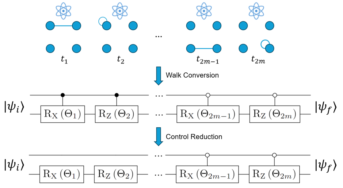
Figure 1: This figure lays out the framework for QSP via quantum walks. Alternating single edge quantum walks with self-loop quantum walks, allows arbitrary QSP. We provide conversion methods to construct the gate based circuit. Control reduction is a method for reducing controls that we introduce in this paper.

Our method builds on the idea of exploiting sparsity to increase the efficiency of QSP techniques by approaching the problem from the perspective of dynamic quantum walks. As such, our method is best suited for the asymptotically sparse states ($m=\mathcal{O}(poly(n))$), but can, in principle, also work for the asymptotically dense states ($m=\mathcal{O}(2^{n})$). The walk framework that we present here is flexible, scalable, and intuitive, building upon well-established graph-based algorithms to efficiently prepare arbitrary quantum states.

This paper is organized as follows. First, we introduce necessary background information and previous works in QSP in Sec. II. We then introduce an algorithm that converts CTQWs on single edge dynamic graphs and single self loop graphs to the circuit model in Sec. III. In Sec. IV, we introduce a deterministic state preparation algorithm and analyze its circuit complexity. We compare our state preparation methods to the uniformly controlled rotation method [5, 31] used by Qiskit in Sec. V. Finally, we discuss future work in Sec. VI.

II Background

In this section, we provide background information and examples of CTQWs on dynamic graphs and state-of-the-art state preparation circuits.

II.1 Continuous-Time Quantum Walks on Dynamic Graphs

A dynamic graph is defined as a sequence of ordered pairs $\{(G_{i},t_{i})\}_{i=1}^{\ell}$ for some $\ell\in\mathbb{N}$ that consists of unweighted graphs $G_{i}$ and corresponding propagation times $t_{i}$. A CTQW on a dynamic graph is then a CTQW where the first walk is performed on graph $G_{1}$ for time $t_{1}$, followed by a walk on graph $G_{2}$ for time $t_{2}$, and so on until all graphs in the sequence have been walked upon. The final state $\ket{\psi_{\ell}}$ is then given by

$$\ket{\psi_{\ell}}=e^{-iA_{\ell}t_{\ell}}\ldots e^{-iA_{2}t_{2}}e^{-iA_{1}t_{1}}\ket{\psi_{0}}.$$ (1)

where $A_{i}$ is the adjacency matrix for graph $G_{i}$, that is a 0-1 valued symmetric matrix. For simplicity, we assume that each graph has $2^{n}$ vertices for some $n\in\mathbb{N}$, and each vertex represents a computational basis state.

As an example, consider the dynamic graph found in Fig. 2, where the adjacency matrices are

$$A_{1} =\begin{pmatrix}0&0&0&0\\ 0&0&0&0\\ 0&0&0&1\\ 0&0&1&0\end{pmatrix}$$

$$A_{2} =\begin{pmatrix}0&0&0&0\\ 0&0&0&0\\ 0&0&1&0\\ 0&0&0&1\end{pmatrix}$$

Figure 2: Dynamic CTQW implementation of CX gate.

If the walker starts in the initial state $\ket{\psi_{0}}=(a,b,c,d)^{T}$, then the final state of this walker is

$$\ket{\psi_{2}}=\begin{pmatrix}1&0&0&0\\ 0&1&0&0\\ 0&0&i&0\\ 0&0&0&i\end{pmatrix}\begin{pmatrix}1&0&0&0\\ 0&1&0&0\\ 0&0&0&-i\\ 0&0&-i&0\end{pmatrix}\begin{pmatrix}a\\ b\\ c\\ d\end{pmatrix}=\begin{pmatrix}a\\ b\\ d\\ c\end{pmatrix}$$

which is equivalent to a CX gate in the circuit model.

Interestingly, CTQWs on dynamic graphs that correspond to operations in the gate model tend to have a similar form: some phase is added to particular basis states via self-loops on vertices of the graph, then they are connected by edges to allow for state transfer, followed by additional self-loops to eliminate unwanted phase. This general alternating sequence of graphs inspires the state preparation algorithm introduced later in this work.

II.2 Prior State Preparation Results

Due to its fundamental role in quantum algorithms [32, 33, 34], quantum state preparation is an active area of research within the space of quantum computation. The resource overhead of general QSP problems for arbitrary states is known to be $\mathcal{O}(2^{n})$ in the number of CX gates [5, 31]. Within this limit, there are different techniques utilizing different resources, which can be useful depending on the context. For instance, if depth is more of a concern than space, Ref. [35] provides an $\mathcal{O}(n^{2})$ depth divide-and-conquer method to prepare arbitrary states at the cost of needing $\mathcal{O}(2^{n})$ ancillary qubits. For arbitrary QSP, the state of the art deterministic protocol achieves $\mathcal{O}(\frac{23}{24}2^{n})$ CX scaling on even numbers of qubits [36]. The downside of this method is that it relies on the Schmidt decomposition of the $n$-qubit target state, a computationally expensive task, which has a classical run time of $\mathcal{O}(2^{3n/2})$ [37].

While arbitrary state preparation is exponential, there are states of practical interest that do not require exponential resources, even in the worst case [38, 39]. Manual methods are strategies for QSP that use advanced knowledge of the target state to save resources in ways that might not be obvious when preparing arbitrary states. For example, GHZ states are highly entangled, but only require a linear number of CX gates. Similarly, the methods introduced in [40] require $\mathcal{O}(kn)$ CX gates to prepare $n$-qubit Dicke states of Hamming weight $k$. For machine learning applications on classical data, quantum data loaders can prepare sparse amplitude encodings of $d$-dimensional real-valued vectors on $d$-qubits in $\mathcal{O}(\log d)$ circuit depth [41]. In Ref. [42], Zhang et al. introduce a technique to prepare input states to the HHL algorithm [3] based on the finite element method equations relevant to electromagnetic problems. Zhang et al.’s algorithm achieves $\mathcal{O}(n)$ depth scaling by exploiting the symmetry and sparsity of the relevant target states; however, these useful assumptions are not guaranteed for arbitrary states.

The state of the art method for preparing arbitrary sparse states is detailed in [6], which produces circuits with $\mathcal{O}(nm)$ CX gates and runs in $\mathcal{O}(nm^{2}\log(m))$ time classically. This type of method is attractive for real-world applications of quantum computers because they can take advantage of sparsity while still remaining agnostic to particular details of the state. Another method using decision trees [43] has $\mathcal{O}(nm)$ CX gates, but it requires an ancilla qubit. The method in Ref. [44] also achieves $\mathcal{O}(nm)$ CX gates. However, this method is based on Householder reflections and is more complicated than the one introduced in Ref. [6].

III Conversion from CTQW on dynamic graphs to the Circuit Model

A standard basis for any adjacency matrix is given by the set of adjacency matrices corresponding to all single edge walks and all single self-loop walks. We introduce the conversion methods that can construct the gate-based representations for these walks on $n$ qubits. Throughout this paper, the considered states are represented in the standard computational basis set.

III.1 Single Edge CTQW to Circuit Model

The adjacency matrix for a single edge graph connecting basis states $\ket{j}$ and $\ket{k}$ is given by

$$A(j,k)=\ket{j}\!\!\bra{k}+\ket{k}\!\!\bra{j}$$ (2)

and the corresponding CTQW for time $t$ is

$$U(j,k;t)=e^{-itA(j,k)}=\cos(t)(\outerproduct{j}{j}+\outerproduct{k}{k})\\ -i\sin(t)(\ket{j}\!\!\bra{k}+\ket{k}\!\!\bra{j})+\sum_{l\notin\{j,k\}}\outerproduct{l}{l}$$ (3)

This unitary transfers amplitude between states $\ket{j}$ and $\ket{k}$ and leaves all other states untouched.

If $\ket{j}$ and $\ket{k}$ differ in exactly one bit at position $l$, $U(j,k;t)$ is the $(n-1)$-controlled Rx($2t$) gate

$$\text{Rx}(2t)=\begin{pmatrix}\cos(t)&-i\sin(t)\\ -i\sin(t)&\cos(t)\end{pmatrix}$$ (4)

where the target qubit is $l$, and the remaining qubits are either 0- or 1-controls corresponding to the remaining bits of $\ket{j}$ and $\ket{k}$.

If the Hamming distance between $\ket{j}$ and $\ket{k}$ is greater than $1$, using the CRx($2t$) gate is still possible, but requires some extra overhead. First apply a sequence of CX gates where the control is any bit in which $\ket{j}$ and $\ket{k}$ differ and the targets are the other bits in which $\ket{j}$ and $\ket{k}$ differ. Then apply the CRx($2t$) gate as before and apply the reverse of the conjugating CX sequence. An example conversion of a single edge walk to gates is shown in Fig. 3. The first CX gate transforms the two basis states such that their Hamming distance becomes equal to 1. The CRx creates the superposition and the final CX restores the original basis states.

The $(n-1)$-controlled CRx gate is a multi-controlled special unitary, and can be decomposed in $\mathcal{O}(n)$ CX and single-qubit gates [45].

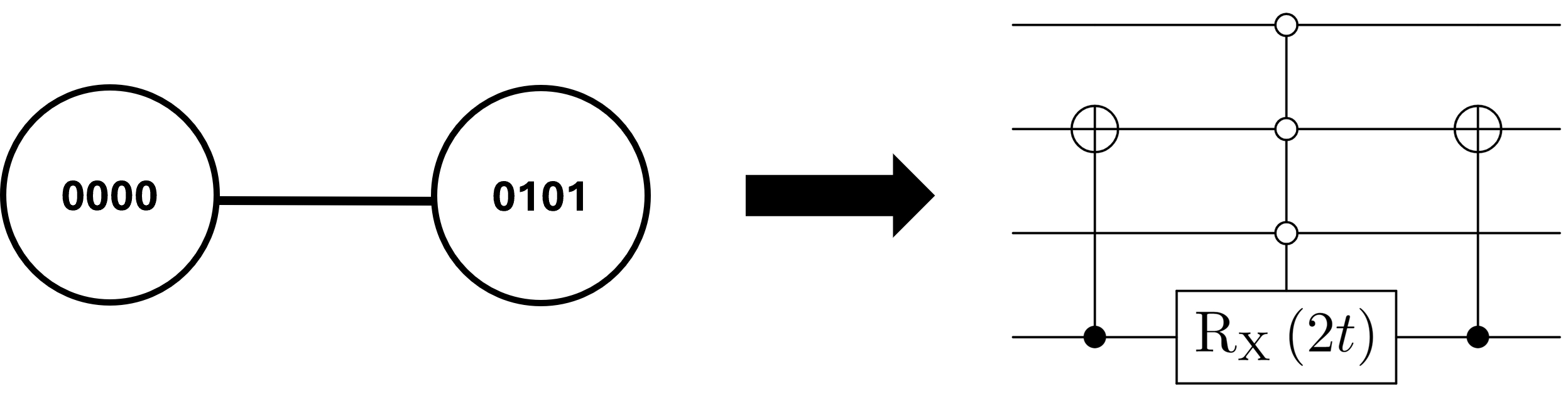
Figure 3: When a single edge walk is between states with non-unit Hamming distance from each other, CX gates might be required in addition to the CRx gate.

III.2 Single Self-Loop CTQW to Circuit Model

A single self-loop walk on basis state $\ket{j}$ is given by the adjacency matrix

$$A(j)=\outerproduct{j}{j},$$ (5)

The corresponding CTQW for time $t$ is

$$U(j;t)=e^{-itA(j)}=e^{-it}\outerproduct{j}{j}+\sum_{k\neq j}\outerproduct{k}{k},$$ (6)

which is a diagonal matrix with a single non-unit element on the diagonal.

From this equation, one can see that the self-loop walk on a single vertex is equivalent to adding phase to exactly one computational basis state. This operation corresponds to an application of an $(n-1)$-controlled phase gate P for time $-t$

$$\text{P}(t)=\begin{pmatrix}1&0\\ 0&e^{it}\end{pmatrix},$$ (7)

where the target qubit can be arbitrarily chosen among the bits of $j$ that are equal to 1 (or 0, with the appropriate X conjugation), and the remaining qubits are either 0- or 1-controls corresponding to the remaining bits of $\ket{j}$.

However, the $\text{P}(t)$ gate is not a special unitary. As such, without using ancilla qubits, its decomposition requires $\mathcal{O}(n^{2})$ CX gates [46]. A more efficient (but also more nuanced) approach is to use an $(n-1)$-controlled Rz($2t$) gate

$$\text{Rz}(2t)=\begin{pmatrix}e^{-it}&0\\ 0&e^{it}\end{pmatrix}$$ (8)

which is a special unitary and can be decomposed in $\mathcal{O}(n)$ CX gates [45].

At a first glance, an $(n-1)$-controlled Rz gate affects two adjacent computational basis states, which makes it not equivalent to a self-loop walk in general. However, if only one of these two basis states exists in the state affected by the CRz gate, then it becomes essentially equivalent to the CP gate and can also be used to implement a self-loop walk.

As long as the state we apply the walk to ($\ket{\psi_{0}}$ in Eq. 1) has at least one zero-amplitude basis state $\ket{z}$, not necessarily adjacent to $\ket{j}$, one can use the same CX conjugation technique as described in the previous section for the Rx gate. This enables the interaction between $\ket{j}$ and $\ket{z}$ via the CRz gate and implements the self-loop walk on $\ket{j}$.

In the case when $\ket{\psi_{0}}$ is fully dense, i.e. all $2^{n}$ basis states have non-zero amplitudes, the above method will not work and a CP gate will have to be used instead.

III.3 Universal Computation

As it was mentioned in the Introduction, CTQWs on dynamic graphs are known to be universal [17]. However, the authors of Ref. [17] use walks on arbitrary graphs in their proof of universality. In this section we prove that using only single edge and single self-loop walks is sufficient to decompose an arbitrary unitary.

Proposition 1.

An arbitrary $d\times d$ unitary can be decomposed into a series of single self-loop and single edge CTQWs.

Proof.

The case of $d=1$ is trivial so we consider $d\geq 2$. An arbitrary unitary can be decomposed into a series of 2-level unitaries (unitaries that act non-trivially on two or fewer basis states, pages 189-191 of [47]).

Similarly to how an arbitrary single-qubit unitary can be decomposed as $U=W(\alpha)\text{Rz}(\beta)\text{Rx}(\gamma)\text{Rz}(\delta)$ (page 175 of [47]), where $W=e^{i\alpha}I$, an arbitrary 2-level unitary $U$ can be decomposed as

$$U=\text{W'}(\alpha)\text{Rz'}(\beta)\text{Rx'}(\gamma)\text{Rz'}(\delta)$$ (9)

for some real numbers $\alpha,\beta,\gamma,\delta$, where the W’, Rz’ and Rx’ are 2-level unitaries whose action in the corresponding 2D subspace is equivalent to their single-qubit counterparts.

As it was shown in Sections III.1 Eq. (3) and III.2 Eq. (6), a single edge CTQW corresponds to Rx’, and a sequence of two single self-loop CTQWs corresponds to W’ and Rz’. Thus, an arbitrary unitary can be decomposed into a series of single self-loop CTQWs and single edge CTQWs.

∎

IV Deterministic state preparation via quantum walks

The above conversions allow one to write single edge walk dynamics and single self-loops in terms of the circuit model. In this section, we describe how a series of such quantum walks can be used to prepare an arbitrary quantum state.

IV.1 General Approach

Given the task of preparing a quantum state with $m<2^{n}$ non-zero amplitudes on $n$ qubits, we start by presenting a high-level description of the algorithm to accomplish this task:

1. Create a tree graph connecting the non-zero amplitudes, as shown in Fig. 4.

2. Starting from an arbitrarily chosen root, and following a graph traversal order, perform a self-loop walk for each encountered node and a single edge quantum walk for each encountered edge.

3. Convert the sequence of the quantum walks to the circuit representation.

Initially, the system starts with all amplitude in the root state, which can be constructed from the ground $\ket{0}$ state simply by applying the X gates to the necessary qubits. The graph traversal order can be be determined by any graph traversal algorithm, such as Depth First Search or Breadth First Search.

An arbitrary amount of amplitude (absolute value) from the source can be transferred to the destination for any pair of the connected states corresponding to each single edge walk, and all non-zero amplitude states are connected transitively via a tree. Therefore, an arbitrary distribution of absolute values of amplitude (but not phases) can be established on the set of non-zero amplitude basis states via single edge walks.

Each self-loop walk on a basis state $\ket{z_{i}}$ establishes the correct phase of the corresponding coefficient $c_{i}$, but does not change the absolute value of it. Therefore, performing self-loop walks on each non-zero amplitude basis state establishes the correct phases of the corresponding coefficients, without interfering with the absolute values established by the single edge walk. Therefore, an arbitrary quantum state can be prepared with a sequence of single edge walks and self-loop walks, as described in the algorithm above.

In the context of the state preparation, CRz gates can easily be used instead of CP gates to implement the self-loop walks, since every single edge walk transfers the amplitude to a new basis state with zero amplitude. Thus, as described in the previous section, the same basis state can be used to establish the correct phase on the source state for the single edge walk without additional CX conjugations. However, this will not apply to the leaf nodes (degree one vertices) in the tree, which will require another zero-amplitude state to interact with.

The tree contains $\mathcal{O}(m)$ nodes and edges, therefore $\mathcal{O}(m)$ walks will be required. As described in the previous section, each walk is represented by a single multi-controlled gate (CRz or CRx) that has up to $n-1$ controls. Each such gate can be implemented in $\mathcal{O}(n)$ CX gates [45] and may need to be conjugated by $\mathcal{O}(n)$ additional CX gates due to the Hamming distance between the adjacent basis states. Therefore the overall complexity of the algorithm, in terms of the required number of CX gates, is $\mathcal{O}(nm)$.

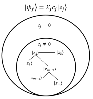
Figure 4: Although there are exponentially many basis states in a generic quantum state, when only a few have non-zero amplitude, a tree over the relevant states can be found with reasonable overhead.

IV.2 Control Reduction

The number of CX gates necessary to implement the multi-controlled Rz and Rx gates is proportional to the number of controls on those gates. As mentioned earlier, we might need up to $n-1$ controls in the worst case, but depending on the walk that we want to implement and the basis states that we have already visited, we might need less than that. For example, when we perform the first walk from the root, we never need any controls, since there are no other basis states that would be affected by the Rx gate.

More generally,

Proposition 2.

Let $n$ denote the number of qubits and $S=\{\ket{z_{1}},\ket{z_{2}},...,\ket{z_{k}}\}$ denote the set of visited nodes. Suppose we wish to perform a single edge walk from $\ket{z_{j}}\in S$ to $\ket{z_{\ell}}\notin S$ and $\ket{z_{j}}$ and $\ket{z_{\ell}}$ have a Hamming distance of 1. Let $b$ denote the qubit where $\ket{z_{j}}$ is different from $\ket{z_{\ell}}$, i.e. $z_{j}[b]\neq z_{\ell}[b].$ Let $D=\{\{k\,|\,z_{i}[k]\neq z_{j}[k],k\neq b\}\,|\,z_{i}\in S\setminus z_{j}\}$ denote the set of differing bits of the visited nodes with $z_{j}$ excluding the qubit $b$. For the gate-based representation of a single edge walk from basis state $\ket{z_{j}}$ to $\ket{z_{\ell}}$, it is sufficient to control the CRz or CRx gate on any hitting set of $D$, where the values of controls are equal to the corresponding bits of $z_{j}$. A hitting set of $D$ is a collection of elements $h$ such that $h\cap d_{i}\neq\emptyset$ for all $d_{i}\in D$.

Proof.

Adding a control on an arbitrary qubit $c$ to any gate makes the gate act only on the states conforming to the value of that control, i.e. $\ket{z_{k}}$ such that $z_{k}[c]=0$ or 1, depending on the state of the control. By the definition of $d_{i}\in D$, controlling the CRz or CRx gate on any index $e\in d_{i}$ with the value of control equal to $z_{j}[e]$ will ensure that the gate does not act on $z_{i}$. Thus, controlling on any hitting set of $D$ will ensure that that the gate does not act on all $z_{i}\in S$, except $z_{j}$. ∎

When $z_{j}$ and $z_{\ell}$ have a Hamming distance greater than 1, we first have to update $S\rightarrow\tilde{S}$ with the conjugating CX gates, as described in Sec. III.1. Then we apply the previously described control reduction method to $\tilde{S}$.

In order to minimize the number of controls, one needs to minimize the size of the hitting set, i.e. solve the minimum hitting set problem, which is known to be NP-complete. As such, no polynomial algorithm is known to solve it exactly, but a number of heuristics exist that can provide good suboptimal solutions quickly [48, 49]. In practice, solving this problem for each walk drastically reduces the number of control qubits on many gates in the sequence (see Fig. 5).

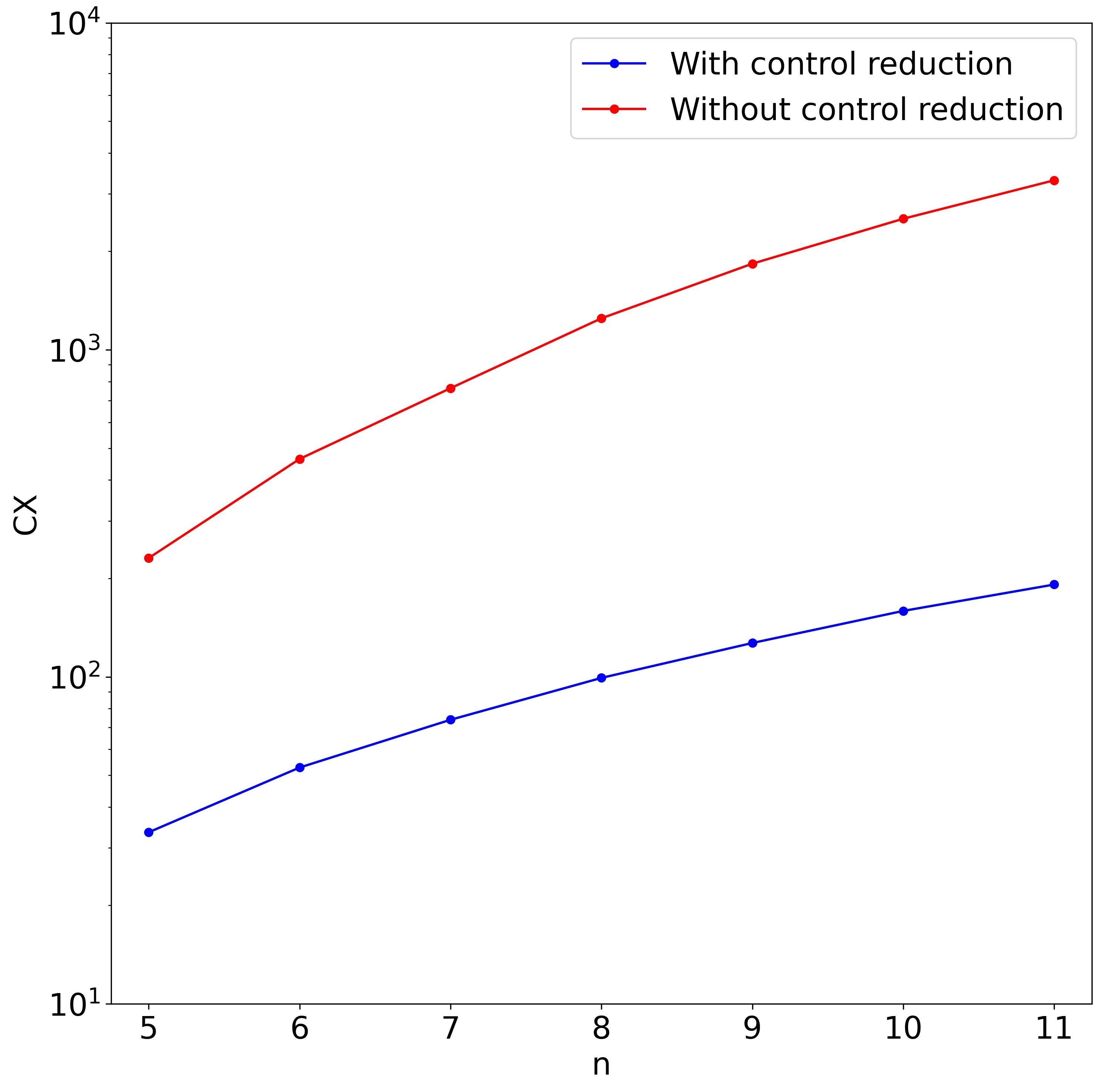
Figure 5: The average number of CX gates necessary to implement a random state with $n$ qubits with and without control reduction. Each state consist of $m=n$ non-zero amplitudes and each point is the average over 1000 random states.

IV.3 Walk Order

Any tree constructed in the first step is, in principle, sufficient for state preparation but not all trees result in the same CX gate count. As mentioned in the previous section, the cost of a walk between a given pair of basis states depends on the Hamming distance between them. Therefore, connecting the basis states that are close to one another (in terms of their Hamming distance) minimizes the number of CX gates in the resulting circuit. Let us consider some of the more advantageous options.

Minimum Spanning Tree. The most straightforward option to minimize the Hamming distance between the connected basis states is to build a Minimum Spanning Tree (MST) over the complete graph of target basis states, where each edge is weighted by the Hamming distance between its endpoints.

The cost of calculating all pairwise Hamming distances is $\mathcal{O}(nm^{2})$, while the MST itself can be built in $\mathcal{O}(m^{2})$ with Prim’s algorithm. Thus, the overall classical complexity for this method is $\mathcal{O}(nm^{2})$.

In the case when the target state is fully dense, i.e. $m=2^{n}$, this method can be simplified, since the tree can be automatically built without calculating all pairwise distances by branching off sequentially in each dimension of the hypercube (see Fig. 6b). The same method can also be used for generally dense states, i.e. when $m=\mathcal{O}(2^{n})$. In this case, the resulting tree will go through some zero-amplitude states, which is not optimal for the circuit, but allows to save classical computational resources.

Shortest Hamiltonian Path. MST approach minimizes the total Hamming distance for the walks, which corresponds to the optimal walk order if control reduction is not taken into account. However, when control reduction is applied, other walk orders may be more efficient since they may allow for additional control reduction.

In general, it is difficult to calculate in advance which walk orders are better for the maximum control reduction, but from the numerical experiments we discovered that, on average, path graphs (trees with exactly two leaves) are more amenable to it than other trees. Therefore, instead of MST, one could find the Shortest Hamiltonian Path (SHP) in the same graph of the target basis states as used to build the MST.

This option is more computationally expensive, since the cost of finding SHP exactly is $\mathcal{O}(m!)$. However, approximate SHP heuristics can find suboptimal solutions much faster [50].

Similar to MST, when $m=2^{n}$ the procedure can be simplified by building a Hamiltonian path throughout the whole hypercube of basis states without calculating all pairwise distances. This path is the known as the Gray code. Examples of the quantum walks produced by SHP for the cases of sparse and dense states are shown in Fig. 6.

Sorted order. Another method to build a simple linear path without solving SHP is to connect the basis states sequentially in increasing order. This method is less optimal than SHP, but it is computationally inexpensive since the target basis states can be sorted in $\mathcal{O}(nm\log(m))$, and can provide us with a reasonably good walking order. For example, for a fully dense state, the average Hamming distance given by the sorted walk order is 2, which is much better than $n/2$ achieved by a random walk order.

A comparison of the different walking orders presented in this section for the case of $m=n$ with control reduction is shown in Fig. 7. We empirically validate the four quantum walk order methods and find that on the prepared states, SHP requires the fewest CX gates, although it approaches the MST method as $n$ increases.

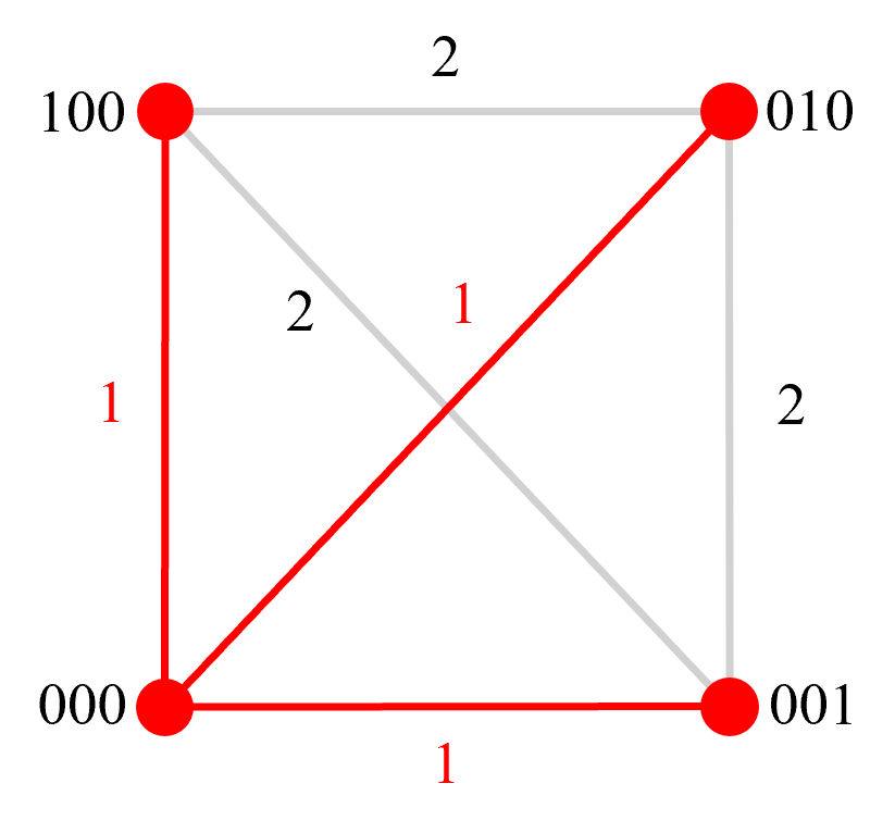
(a) MST for a sparse state.

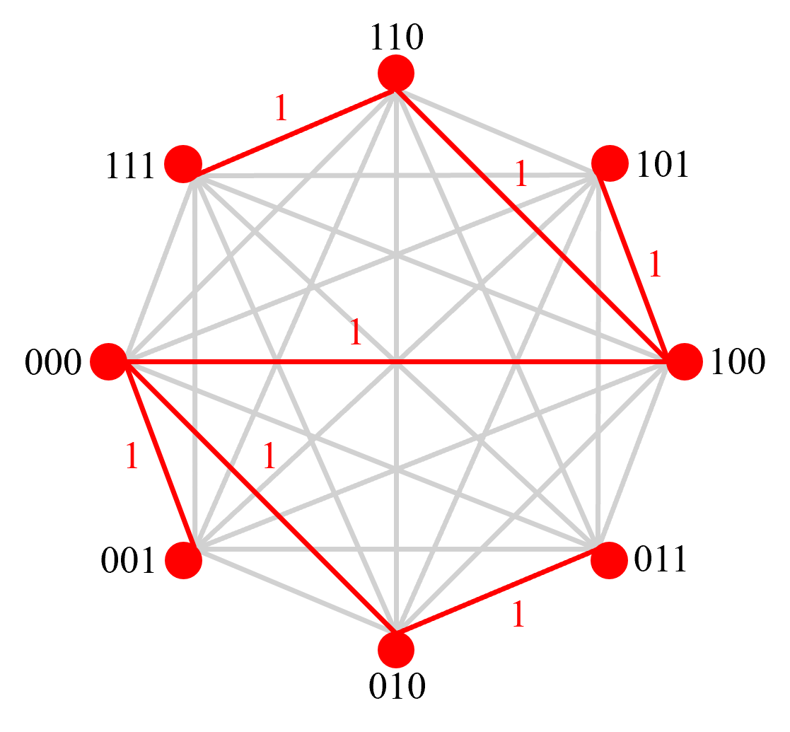
(b) MST for a dense state.

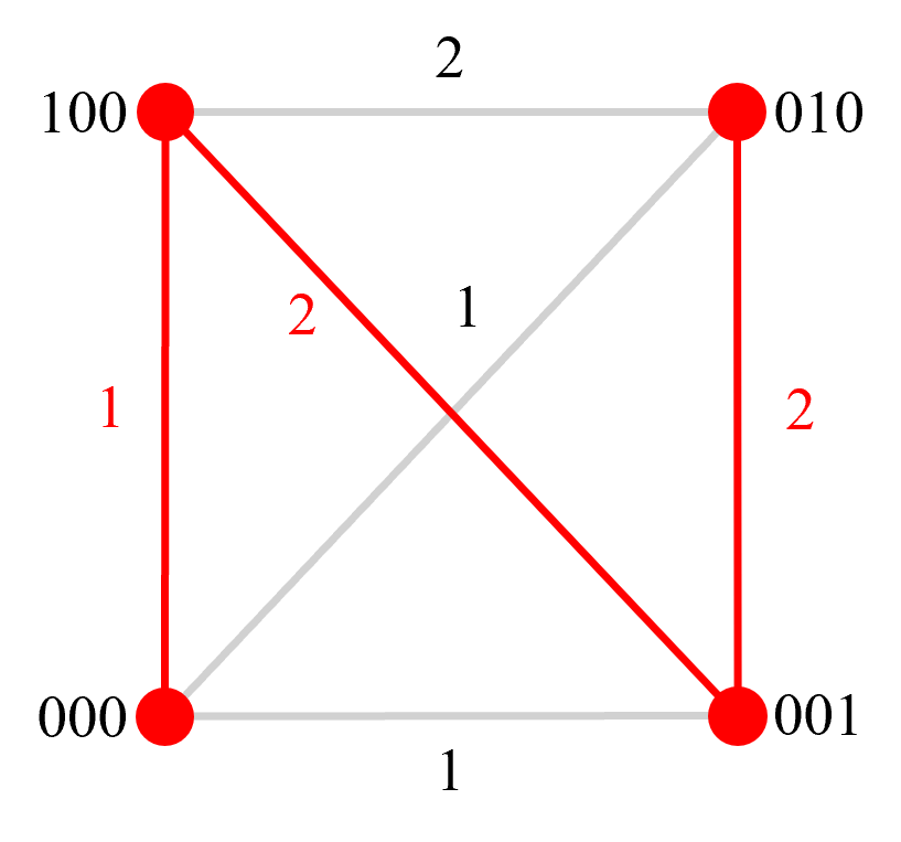
(c) SHP for a sparse state.

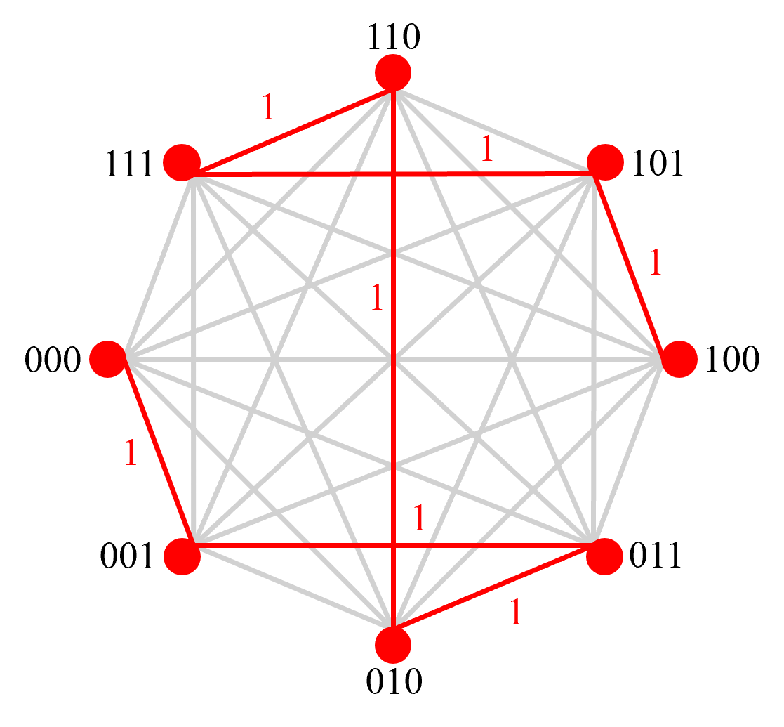
(d) SHP for a dense state.

Figure 6: Example walks generated by different methods for the case of 3 qubits. The weight of an edge is the Hamming distance of the two nodes. A potential walk path chosen by a given method is shown in red. In Figs. 6d and  6b, the costs of the edges are suppressed except for the path.

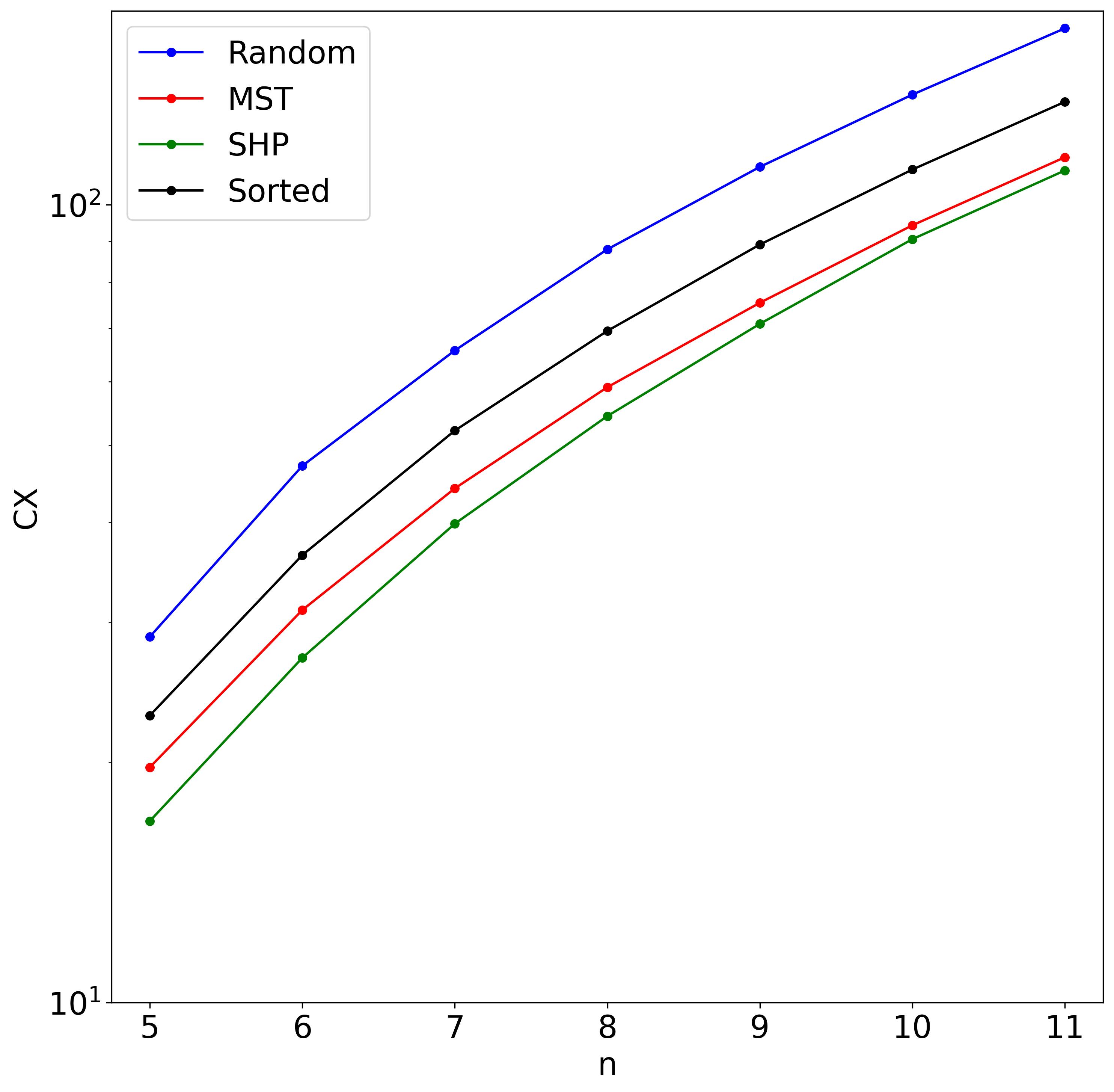
Figure 7: The average number of CX gates necessary to implement a random state with given number of qubits for the considered walk orders. Each state consist of $m=n$ non-zero amplitudes and each point is the average over 1000 random states.

IV.4 Additional Optimizations

A single edge between states $\ket{j}$ and $\ket{k}$ corresponds to a CRx gate, which introduces an imaginary phase on $\ket{k}$. However, for the purpose of preparing a state with some real-valued amplitudes, a better approach is to use a CRy gate instead, which has the same action as CRx, except it does not introduce a complex phase. CRy keeps the amplitudes real and makes it unnecessary to use CRz or CP gates when the amplitude is transferred between the basis states with real coefficients. As such, for these states, one might want to use a special walk order that goes through all real-valued basis states before moving to the complex-valued ones. For the states where all amplitudes are real, this approach can reduce the total number of CX gates in the circuit by a factor of approximately 2. We plan to implement this in our code in the future.

IV.5 Example

Suppose we want to prepare the state

$$\ket{\psi}=c_{1}\ket{00001}+c_{2}\ket{00110}+c_{3}\ket{00111}\\ +c_{4}\ket{01001}+c_{5}\ket{01011}$$ (10)

Using the algorithm described above, with sorted walk order and control reduction, one can generate a circuit shown in Fig. 8. The exact values of the coefficients $c_{1},...,c_{5}$ can be disregarded here, since they only change the angles of the rotational gates, but not the overall structure of the circuit.

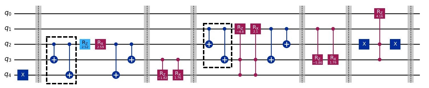
Figure 8: Example circuit generated by the quantum walk state preparation algorithm presented in this work. The leading CX gates in the dashed rectangles can be removed without affecting the final state.

First, we start from the $\ket{00001}$ state by applying an X gate to the last qubit. In the second segment of the circuit, we want to connect with the state $\ket{00110}$. This state is different from the previous state in bits 2, 3, and 4. We arbitrarily choose qubit 2 as the target qubit and make the other bits consistent by applying CX gates to qubits 3 and 4, with control on qubit 2, which transforms the $\ket{00110}$ state to $\ket{00101}$. This enables the quantum walks between the states $\ket{00001}$ and $\ket{00101}$, which consist of the Rz gate that establishes the correct phase of $c_{1}$, and Rx gate, which establishes the correct magnitude of $c_{1}$. No controls are necessary on Rz and Rx gates here since only one state has non-zero amplitude at this point. After that, we apply the same CX gates again to transform the newly populated state back to $\ket{00110}$.

In segment 3, we want to connect the states $\ket{00110}$ and $\ket{00111}$. These states are already adjacent, so no CX conjugation is necessary here. We want to make sure that Rz and Rx gates only affect $\ket{00110}$ and not $\ket{00001}$, so we add the minimally necessary number of controls to make it happen. In this case, it is sufficient to control on qubit 3. After these operations, the correct phase and magnitude of $c_{2}$ are established.

Continuing in the same fashion, we connect the states $\ket{00111}$ and $\ket{01001}$ in segment 4, and states $\ket{01001}$ and $\ket{01011}$ in segment 5. After this, all phases and magnitudes of the target coefficients are correct, except for the phase of $c_{5}$. To fix the phase of $c_{5}$, we choose the closest zero-amplitude state to the last populated state and interact with it via the Rz gate (no Rx gate is needed here). In this case, we chose the state $\ket{11011}$ and control on qubits 2 and 3, where the control on qubit 2 is conjugated with X gates to implement a 0-control.

Note that the leading CX gates, marked with the dashed rectangles in Fig. 8 can be removed, since their control qubits, at the time of the gate application, are guaranteed to be in the 0-state. This optimization can only be done at the beginning of the circuit, before any CRx gates acted on the corresponding qubits, therefore we show these gates here for the purpose of demonstrating a general circuit structure.

V Performance

We tested the validity of our method by preparing 1000 random quantum states for each combination of $n$ and $m$ shown in Fig. 9. Each state was prepared using the quantum walk based techniques presented in this work with control reduction and SHP walk order. Additionally, the same states were also prepared with Qiskit’s built-in prepare_state method (which is based on Ref. [31]), shown here for comparison. All circuits have been transpiled into single-qubit gates and CX basis using Qiskit’s transpiler with optimization level 3.

As can be seen from Fig. 9, Qiskit’s performance scales exponentially and is very similar regardless of the value of $m$. In fact, for $m=n^{2}$ and $m=2^{n-1}$ Qiskit produces circuits with exactly the same number of CX gates regardless of the state being prepared.

In contrast to Qiskit, our method takes advantage of the sparsity of the target state and is expected to outperform Qiskit’s built-in method for any asymptotically sparse state (i.e. $m=\mathcal{O}(poly(n))$) for sufficiently large values of $n$. However, for asymptotically dense states (i.e. $m=\mathcal{O}(2^{n})$) our method is less efficient than Qiskit for sufficiently large values of $n$.

The exact code and data for these numerical experiments can be found in the linked repository (see Data Availability section Code and Data Availability).

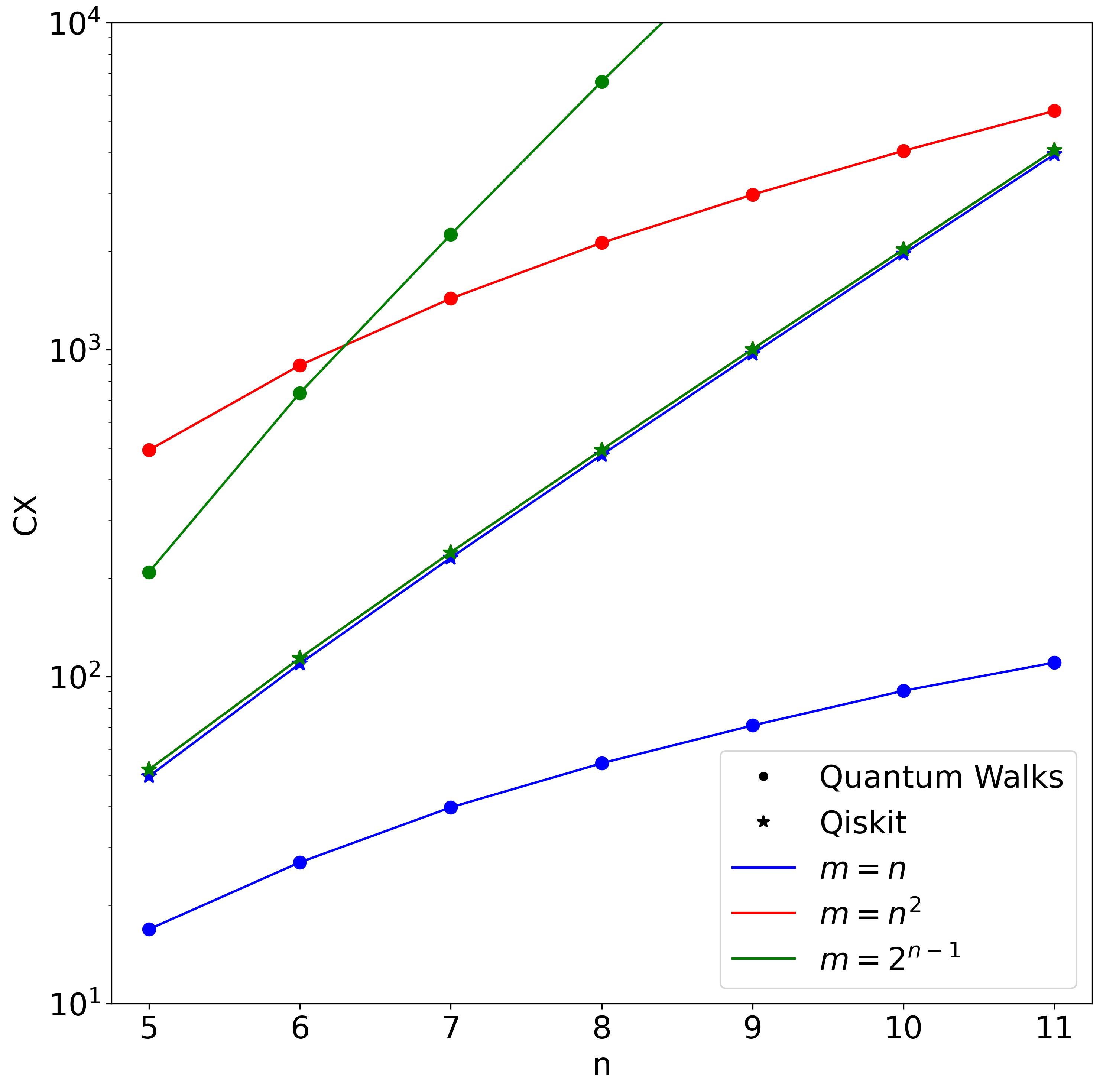
Figure 9: The average number of CX gates necessary to prepare a random state using the uniformly controlled rotation method [31] used by Qiskit’s built-in state preparation algorithm and the quantum-walk based algorithm presented in this paper for different values of $n$ and $m$.

VI Conclusions and Future Directions

In this work, we developed an algorithm that can be used to convert CTQWs on dynamic graphs that consist only of self-loops or single edges to the quantum gate model. This algorithm serves as the basis for a deterministic state preparation routine that has complexity $\mathcal{O}(nm)$ where $n$ is the number of qubits and $m$ is the number of basis states in the target state. Furthermore, we introduce multiple methods that can reduce the CX count of the state preparation algorithm and test these methods against the uniformly controlled rotation method [31] used by the Qiskit transpiler. We find that our state preparation methods require fewer CX gates when the target state has a polynomial number of non-zero amplitudes.

The quantum walks QSP framework we present posts many interesting possible avenues for future investigation. As mentioned in Sections IV.2 and IV.3, the gate count for preparing an arbitrary state can be reduced depending on the order in which the state transfer occurs. Without control reduction, the optimal sequence of walks is given by the minimum spanning tree approach. Determining the optimal sequence of basis state transfers in the presence of control reduction is more complicated and could be an interesting direction for future research. Additionally, if a target state is comprised of basis states with symmetry, it may be possible to cleverly reduce the number of gates required to create the target state by exploiting symmetry. Another interesting avenue for future work is to compare against the methods in Refs. [6, 44].

Author contributions

AG developed the CTQWs to gates conversion, formulated control reduction, wrote code, gathered data, constructed proofs, and calculated complexities. RH developed the algorithm that converts CTQWs on dynamic graphs to the circuit model. CC wrote code, developed state preparation approaches, and tested circuit optimization techniques. IG developed the minimum spanning tree approach, CRz implementation of the self-loop walks, wrote code, collected data and prepared some figures. JL also developed the circuit optimization for reducing control bits. TT helped develop state preparation approaches and evaluation methodology. ZHS had the idea of creating a dictionary between single edge quantum walks and quantum circuits.

All authors wrote, read, edited, and approved the final manuscript.

Competing interests

All authors declare no financial or non-financial competing interests.

Code and Data Availability

The code and data for this research can be found at https://github.com/GaidaiIgor/quantum_walks.

The submitted manuscript has been created by UChicago Argonne, LLC, Operator of Argonne National Laboratory (“Argonne”). Argonne, a U.S. Department of Energy Office of Science laboratory, is operated under Contract No. DE-AC02-06CH11357. The U.S. Government retains for itself, and others acting on its behalf, a paid-up nonexclusive, irrevocable worldwide license in said article to reproduce, prepare derivative works, distribute copies to the public, and perform publicly and display publicly, by or on behalf of the Government. The Department of Energy will provide public access to these results of federally sponsored research in accordance with the DOE Public Access Plan. http://energy.gov/downloads/doe-public-access-plan.

References

- [1] Ashley Montanaro. Quantum speedup of monte carlo methods. Proceedings of the Royal Society A: Mathematical, Physical and Engineering Sciences, 471(2181):20150301, 2015.
- [2] Peter W Shor. Polynomial-time algorithms for prime factorization and discrete logarithms on a quantum computer. SIAM review, 41(2):303–332, 1999.
- [3] Aram W Harrow, Avinatan Hassidim, and Seth Lloyd. Quantum algorithm for linear systems of equations. Physical review letters, 103(15):150502, 2009.
- [4] Ryan LaRose and Brian Coyle. Robust data encodings for quantum classifiers. Physical Review A, 102(3):032420, 2020.
- [5] Mikko Möttönen, Juha J. Vartiainen, Ville Bergholm, and Martti M. Salomaa. Transformation of quantum states using uniformly controlled rotations. Quantum Info. Comput., 5(6):467–473, sep 2005.
- [6] Niels Gleinig and Torsten Hoefler. An efficient algorithm for sparse quantum state preparation. In 2021 58th ACM/IEEE Design Automation Conference (DAC), pages 433–438, 2021.
- [7] Andrew M Childs. Universal computation by quantum walk. Physical review letters, 102(18):180501, 2009.
- [8] Edward Farhi and Sam Gutmann. Quantum computation and decision trees. Physical Review A, 58(2):915, 1998.
- [9] Andrew M Childs and Jeffrey Goldstone. Spatial search by quantum walk. Physical Review A, 70(2):022314, 2004.
- [10] Enrico Scalas. The application of continuous-time random walks in finance and economics. Physica A: Statistical Mechanics and its Applications, 362(2):225–239, 2006.
- [11] Oliver Mülken and Alexander Blumen. Continuous-time quantum walks: Models for coherent transport on complex networks. Physics Reports, 502(2-3):37–87, 2011.
- [12] Brian Berkowitz, Andrea Cortis, Marco Dentz, and Harvey Scher. Modeling non-fickian transport in geological formations as a continuous time random walk. Reviews of Geophysics, 44(2), 2006.
- [13] Xiaogang Qiang, Xuejun Yang, Junjie Wu, and Xuan Zhu. An enhanced classical approach to graph isomorphism using continuous-time quantum walk. Journal of Physics A: Mathematical and Theoretical, 45(4):045305, 2012.
- [14] Robert J Chapman, Matteo Santandrea, Zixin Huang, Giacomo Corrielli, Andrea Crespi, Man-Hong Yung, Roberto Osellame, and Alberto Peruzzo. Experimental perfect state transfer of an entangled photonic qubit. Nature communications, 7(1):11339, 2016.
- [15] Xiaogang Qiang, Thomas Loke, Ashley Montanaro, Kanin Aungskunsiri, Xiaoqi Zhou, Jeremy L O’Brien, Jingbo B Wang, and Jonathan CF Matthews. Efficient quantum walk on a quantum processor. Nature communications, 7(1):11511, 2016.
- [16] Hao Tang, Xiao-Feng Lin, Zhen Feng, Jing-Yuan Chen, Jun Gao, Ke Sun, Chao-Yue Wang, Peng-Cheng Lai, Xiao-Yun Xu, Yao Wang, et al. Experimental two-dimensional quantum walk on a photonic chip. Science advances, 4(5):eaat3174, 2018.
- [17] Rebekah Herrman and Travis S Humble. Continuous-time quantum walks on dynamic graphs. Physical Review A, 100(1):012306, 2019.
- [18] Thomas G Wong. Isolated vertices in continuous-time quantum walks on dynamic graphs. Physical Review A, 100(6):062325, 2019.
- [19] Rebekah Herrman and Thomas G Wong. Simplifying continuous-time quantum walks on dynamic graphs. Quantum Information Processing, 21(2):54, 2022.
- [20] Ibukunoluwa A Adisa and Thomas G Wong. Implementing quantum gates using length-3 dynamic quantum walks. Physical Review A, 104(4):042604, 2021.
- [21] Edward Farhi, Jeffrey Goldstone, and Sam Gutmann. A quantum approximate optimization algorithm. arXiv preprint arXiv:1411.4028, 2014.
- [22] Linghua Zhu, Ho Lun Tang, George S Barron, FA Calderon-Vargas, Nicholas J Mayhall, Edwin Barnes, and Sophia E Economou. Adaptive quantum approximate optimization algorithm for solving combinatorial problems on a quantum computer. Physical Review Research, 4(3):033029, 2022.
- [23] Xiaoyuan Liu, Ruslan Shaydulin, and Ilya Safro. Quantum approximate optimization algorithm with sparsified phase operator. In 2022 IEEE International Conference on Quantum Computing and Engineering (QCE), pages 133–141. IEEE, 2022.
- [24] Anthony Wilkie, Igor Gaidai, James Ostrowski, and Rebekah Herrman. Qaoa with random and subgraph driver hamiltonians. arXiv preprint arXiv:2402.18412, 2024.
- [25] Rebekah Herrman, Phillip C Lotshaw, James Ostrowski, Travis S Humble, and George Siopsis. Multi-angle quantum approximate optimization algorithm. Scientific Reports, 12(1):6781, 2022.
- [26] Igor Gaidai and Rebekah Herrman. Performance analysis of multi-angle qaoa for . arXiv preprint arXiv:2312.00200, 2023.
- [27] Kaiyan Shi, Rebekah Herrman, Ruslan Shaydulin, Shouvanik Chakrabarti, Marco Pistoia, and Jeffrey Larson. Multiangle qaoa does not always need all its angles. In 2022 IEEE/ACM 7th Symposium on Edge Computing (SEC), pages 414–419. IEEE, 2022.
- [28] Alberto Peruzzo, Jarrod McClean, Peter Shadbolt, Man-Hong Yung, Xiao-Qi Zhou, Peter J Love, Alán Aspuru-Guzik, and Jeremy L O’brien. A variational eigenvalue solver on a photonic quantum processor. Nature communications, 5(1):4213, 2014.
- [29] Ho Lun Tang, VO Shkolnikov, George S Barron, Harper R Grimsley, Nicholas J Mayhall, Edwin Barnes, and Sophia E Economou. qubit-adapt-vqe: An adaptive algorithm for constructing hardware-efficient ansätze on a quantum processor. PRX Quantum, 2(2):020310, 2021.
- [30] Xiaoyuan Liu, Anthony Angone, Ruslan Shaydulin, Ilya Safro, Yuri Alexeev, and Lukasz Cincio. Layer vqe: A variational approach for combinatorial optimization on noisy quantum computers. IEEE Transactions on Quantum Engineering, 3:1–20, 2022.
- [31] V.V. Shende, S.S. Bullock, and I.L. Markov. Synthesis of quantum-logic circuits. IEEE Transactions on Computer-Aided Design of Integrated Circuits and Systems, 25(6):1000–1010, 2006.
- [32] Almudena Carrera Vazquez and Stefan Woerner. Efficient state preparation for quantum amplitude estimation. Physical Review Applied, 15(3):034027, 2021.
- [33] Xiao-Ming Zhang, Tongyang Li, and Xiao Yuan. Quantum state preparation with optimal circuit depth: Implementations and applications. Physical Review Letters, 129(23):230504, 2022.
- [34] Bryan T Gard, Linghua Zhu, George S Barron, Nicholas J Mayhall, Sophia E Economou, and Edwin Barnes. Efficient symmetry-preserving state preparation circuits for the variational quantum eigensolver algorithm. npj Quantum Information, 6(1):10, 2020.
- [35] Israel F. Araujo, Daniel K. Park, Francesco Petruccione, and Adenilton J. da Silva. A divide-and-conquer algorithm for quantum state preparation. Scientific Reports, 11(1):6329, Mar 2021.
- [36] Martin Plesch and Časlav Brukner. Quantum-state preparation with universal gate decompositions. Phys. Rev. A, 83:032302, Mar 2011.
- [37] Gene H Golub and Charles F Van Loan. Matrix computations, 1996.
- [38] Diogo Cruz, Romain Fournier, Fabien Gremion, Alix Jeannerot, Kenichi Komagata, Tara Tosic, Jarla Thiesbrummel, Chun Lam Chan, Nicolas Macris, Marc-André Dupertuis, et al. Efficient quantum algorithms for ghz and w states, and implementation on the ibm quantum computer. Advanced Quantum Technologies, 2(5-6):1900015, 2019.
- [39] Andreas Bärtschi and Stephan Eidenbenz. Deterministic Preparation of Dicke States, page 126–139. Springer International Publishing, 2019.
- [40] Andreas Bärtschi and Stephan Eidenbenz. Short-depth circuits for dicke state preparation. In 2022 IEEE International Conference on Quantum Computing and Engineering (QCE), pages 87–96. IEEE, 2022.
- [41] Iordanis Kerenidis, Natansh Mathur, Jonas Landman, Martin Strahm, Yun Yvonna Li, et al. Quantum vision transformers. Quantum, 8:1265, 2024.
- [42] Jianan Zhang, Feng Feng, and Qi-Jun Zhang. Quantum computing method for solving electromagnetic problems based on the finite element method. IEEE Transactions on Microwave Theory and Techniques, 72(2):948–965, 2024.
- [43] Fereshte Mozafari, Giovanni De Micheli, and Yuxiang Yang. Efficient deterministic preparation of quantum states using decision diagrams. Phys. Rev. A, 106:022617, Aug 2022.
- [44] Emanuel Malvetti, Raban Iten, and Roger Colbeck. Quantum Circuits for Sparse Isometries. Quantum, 5:412, March 2021.
- [45] Rafaella Vale, Thiago Melo D. Azevedo, Ismael C. S. Araújo, Israel F. Araujo, and Adenilton J. da Silva. Decomposition of multi-controlled special unitary single-qubit gates, 2023.
- [46] Adenilton J Da Silva and Daniel K Park. Linear-depth quantum circuits for multiqubit controlled gates. Physical Review A, 106(4):042602, 2022.
- [47] Michael A Nielsen and Isaac L Chuang. Quantum Computation and Quantum Information. Cambridge University Press, 2011.
- [48] Staal Vinterbo and Aleksander Øhrn. Minimal approximate hitting sets and rule templates. International Journal of approximate reasoning, 25(2):123–143, 2000.
- [49] Andrew Gainer-Dewar and Paola Vera-Licona. The minimal hitting set generation problem: algorithms and computation. SIAM Journal on Discrete Mathematics, 31(1):63–100, 2017.
- [50] Yuri Gurevich and Saharon Shelah. Expected computation time for hamiltonian path problem. SIAM Journal on Computing, 16(3):486–502, 1987.