Bridging electronic and classical density-functional theory
using universal machine-learned functional approximations

Abstract

The accuracy of density-functional theory (DFT) is determined by the quality of the approximate functionals, such as exchange-correlation in electronic DFT and the excess functional in the classical DFT formalism of fluids. The exact functional is highly nonlocal for both electrons and fluids, yet most approximate functionals are semi-local or nonlocal in a limited weighted-density form. Machine-learned (ML) nonlocal density-functional approximations are promising in both electronic and classical DFT, but have so far employed disparate approaches with limited generality. Here, we formulate a universal approximation framework and training protocol for nonlocal ML functionals, combining features of equivariant convolutional neural networks and the weighted-density approximation. We prototype this approach for several 1D and quasi-1D problems and demonstrate that a functional with exactly the same hyperparameters achieves excellent accuracy for the hard-rod fluid, the inhomogeneous Ising model, the exact exchange functional for electrons, the electron kinetic energy functional for orbital-free DFT, as well as for liquid water with 1D inhomogeneities. These results lay the foundation for a universal ML approach to exact 3D functionals spanning electronic and classical DFT.

I Introduction

Electronic density-functional theory (DFT) has become indispensable in physics, chemistry, and materials science, with its low cost and reasonable accuracy for electronic structure predictions making it a vital component of tens of thousands of scientific publications each year.[1] The accuracy of electronic DFT hinges on the quality of the approximate exchange-correlation functionals, with advances from local, through semi-local to nonlocal functionals gradually improving the reliability and applicability of DFT.[2] Machine learning (ML) has shown promise for accelerating this improvement and more rapidly approaching the in-principle exact DFT functional.[3, 4]

As ubiquitous as electronic DFT has become as an electronic structure method, DFT is a much more general technique that is widely applicable to many-body interacting systems. Classical DFT is a technique in the statistical mechanics of fluids that describes equilibrium properties of inhomogeneous fluids in terms of their density distributions alone, eliminating the need to themrodynamically sample the intractably large configuration space of fluid molecules.[5, 6] This is particularly appealing when combining classical DFT with electronic DFT for capturing the effects of solvents and electrolytes on electronic structure.[7]

However, developing functional approximations for classical DFT is fundamentally more challenging than for the electronic case for two reasons. First, there is one exact exchange-correlation functional that needs approximation, which can then be used for DFT calculations for any material / configuration of atoms. In contrast, classical DFT requires an excess functional approximation to be painstakingly constructed for each liquid or electrolyte of interest. Second, classical DFT functionals are fundamentally more challenging to approximate than exchange-correlation functionals, with semi-local functionals being grossly inadequate. Minimum viable classical DFTs are already nonlocal, starting at the weighted density approximation (WDA) level,[8] extended to the rank-2 decomposition and fundamental measure theory approach,[9, 10] which are then perturbed to develop approximations for real fluids.[11, 12, 13, 14, 15] The complexity of developing the necessary nonlocal functionals has limited the widespread application of classical DFT. ML offers a solution to overcoming this current bottleneck to facilitate the development of such functionals.[16]

ML has had a significant impact in the materials and electronic structure field, ranging from rapid property predictions bypassing DFT, to bypassing solving the KS equations either through the prediction of DFT quantities directly (e.g., electron density),[4, 17] or through predicting the Hamiltonian matrix.[18, 19, 20, 21, 22] Moreover, several ML approaches have been adopted to improve the DFT functionals by developing better semi-local and nonlocal exchange and correlation functionals,[23, 24, 25] as well as for the kinetic energy functional for orbital-free DFT.[3, 26]

Due to fundamental differences in the interactions they approximate, traditional electronic and classical DFT methods adopt distinct approaches. Correspondingly, the applications of ML for functional development have also been disjoint in these two fields, despite a fundamental similarity in the key goal: approximating a functional that maps a density distribution to a scalar, the energy. A unified approach to accelerate functional developments across both fields would therefore be highly desirable.

Here, we show that a single universal approach is promising to develop accurate nonlocal functionals across a wide range of fields, spanning both electronic and classical DFT. Below, we will first briefly describe density functionals in both quantum and classical contexts. Then, we describe our unified framework combining equivariant convolutional neural networks with the weighted-density approximation and establish a general training protocol across different classes of DFTs. Finally, we will apply this universal technique to a diverse set of classical and quantum systems including the 1D hard-rod fluid, the Ising model, Hartree-Fock exchange, the Kohn-Sham kinetic energy and liquid water, and demonstrate excellent accuracy across all of these cases with the same hyperparameters.

II Theoretical Formulation

Density-functional theory is a general theorem that the ground-state energy $E$, or similarly the equilibrium free energies, of a many-body system in an external potential $V(\boldsymbol{\mathbf{r}})$ can be obtained by minimizing a functional of the density $n(\boldsymbol{\mathbf{r}})$ alone, as

$$E=\min_{n(\boldsymbol{\mathbf{r}})}\left[F[n(\boldsymbol{\mathbf{r}})]+\int d\boldsymbol{\mathbf{r}}V(\boldsymbol{\mathbf{r}})n(\boldsymbol{\mathbf{r}})\right],$$ (1)

where $F[n]$ is a universal functional of the density, independent of the potential $V$. Applied to electrons, $F$ is the Hohenberg-Kohn energy functional in the microcanonical ensemble,[27] or the Mermin Helmholtz free-energy functional in the canonical ensemble.[5]

This theorem only requires that the interaction of the many-body system with the external potential takes the form $\int d\boldsymbol{\mathbf{r}}\,V(\boldsymbol{\mathbf{r}})n(\boldsymbol{\mathbf{r}})$, and does not depend on the details of the internal interactions of the system. Applied to a classical fluid with atomic densities $n_{\alpha}(\boldsymbol{\mathbf{r}})$ in external potentials $V_{\alpha}(\boldsymbol{\mathbf{r}})$ and chemical potentials $\mu_{\alpha}$ (in the grand-canonical ensemble), with $\alpha$ indexing species, e.g., O, H for water, the equilibrium grand free energy is

$$\Phi=\min_{n_{\alpha}(\boldsymbol{\mathbf{r}})}\left[F[n_{\alpha}(\boldsymbol{\mathbf{r}})]+\sum_{\alpha}\int d\boldsymbol{\mathbf{r}}(V(\boldsymbol{\mathbf{r}})-\mu_{\alpha})n_{\alpha}(\boldsymbol{\mathbf{r}})\right].$$ (2)

Practical applications of DFT require an approximation of the unknown exact functional $F$. In both electronic and classical DFT, the standard approach is to break out known exact pieces, leaving behind the smallest and hopefully easiest piece to approximate. In electronic DFT in the Kohn-Sham formalism,[28] the exact functional is split as

$$F[n]=T_{S}[\{\psi_{i}[n]\}]+E_{\textrm{H}}[n]+E_{\textrm{xc}}[n],$$ (3)

separating out the exact orbital-dependent kinetic energy of the non-interacting electronic system at the same density $n(\boldsymbol{\mathbf{r}})$ and the mean-field Coulomb interaction $E_{\textrm{H}}$, leaving behind the exchange-correlation functional to approximate. Further, directly approximating $T_{S}[n]$ from the electron density would enable orbital-free DFT, however it is generally very difficult to achieve accuracy comparable to the orbital-dependent version in Kohn-Sham theory. Correspondingly, classical DFT typically partitions the exact functional as

$$F[n_{\alpha}(\boldsymbol{\mathbf{r}})]=F_{\rm id}[n_{\alpha}(\boldsymbol{\mathbf{r}})]+F_{\rm ex}[n_{\alpha}(\boldsymbol{\mathbf{r}})],$$ (4)

separating out the exact ideal gas free energy $F_{\rm id}$ at the same set of densities, leaving behind the excess functional $F_{\rm ex}$ that needs to be approximated.

Conventional approaches to approximate $E_{\textrm{xc}}[n]$, $T_{S}[n]$ and $F_{\rm ex}[n_{\alpha}]$ include semi-local approximations of the form $F[n]=\int d\boldsymbol{\mathbf{r}}\,nf(n,\nabla n)$ and the weighted density approximation (WDA) $F[n]=\int d\boldsymbol{\mathbf{r}}\,nf(w\ast n)$, where the convolution by a weight function $w$ introduces nonlocality. Semi-local approximations are widely applied for $E_{\textrm{xc}}$, but much less successful for $T_{S}[n]$ and grossly inadequate for $F_{\rm ex}$, where at least the WDA is necessary.

II.1 Machine-learning density functionals

Here, we propose universal ML density-functional approximations as a sequence of convolution ($C$) and activation ($A$) layers that ultimately culminates in a readout ($R$) layer,

$$\begin{split}F[n_{\alpha}(\boldsymbol{\mathbf{r}})]=\int d\boldsymbol{\mathbf{r}}\,R(n_{\alpha},\,&C_{\alpha_{m}}[A_{\alpha_{m-1}^{\prime}}(C_{\alpha_{m-1}}[\\ &\cdots A_{\alpha_{1}^{\prime}}(C_{\alpha_{1}}[n_{\alpha}(\boldsymbol{\mathbf{r}})])])]).\end{split}$$ (5)

Here, $\alpha$ label channels in the input and through all the intermediate layers. At the input, these channels are physical indices of the density, such as spin for electrons or atomic site type for a classical fluid (e.g. $O,H$ for water). The intermediate $\alpha_{i}$ label the output channels of each $C$ or $A$ layer, with the number of these layers and the number of $\alpha_{i}$ at each intermediate layer being hyperparameters of the model. Note that the readout $R()$ and activation $A()$ are functions that operate locally in space, while $C[\ ]$ is a functional that is nonlocal in space.

Each input or intermediate $\alpha$ index corresponds to a specific representation of the rotation group of space. In 1D, these indices corresponds to odd or even representations of the $Z_{2}$ group (reflection of the single axis). While in 3D, these indices would correspond to $l$ and $m$ of the spherical harmonics. To rapidly prototype and test the universality of the ML DFT approach across several distinct problems, we focus our applications here on 1D systems, but the overall structure and logic extends straightforwardly to the 3D case, as we will point out briefly for each operator below.

II.1.1 Convolution layers

We define the linear convolution layers as

$$C_{\alpha}[n_{\beta}](\boldsymbol{\mathbf{r}})=\int d\boldsymbol{\mathbf{r}}^{\prime}w_{\alpha\beta}(\boldsymbol{\mathbf{r}}-\boldsymbol{\mathbf{r}}^{\prime})n_{\beta}(\boldsymbol{\mathbf{r}}^{\prime})$$ (6)

with learnable weight functions $w_{\alpha\beta}$. Each input density index $\beta$ corresponds to an even or odd function, and, likewise, each output channel index $\alpha$ also is either even or odd. Correspondingly, each weight function $w_{\alpha\beta}$ is even if $\alpha$ and $\beta$ correspond to the same parity and is odd otherwise. For the 3D case, the mapping from inputs to outputs involves Clebsh-Gordon coefficients to combine the $(l,m)$ and $(l^{\prime},m^{\prime})$ of the inputs and weights into $(L,M)$ of the outputs. The rest of the structure remains unchanged.

To preserve rotational invariance of the energy, the final convolution layer must output only even-weighted densities (or $L=0$ in 3D) for the WDA-style readout function discussed below. See the SI for an alternate readout function motivated from the ‘rank-2 approximation’ form proposed by Percus for classical DFT,[9] which can handle non-scalar weighted densities as inputs. Our numerical tests indicate that the WDA-style readout works more generally, so we focus on this approach here.

The learnable parameters of the convolution layer are within the weight functions, which we define as smooth functions $\tilde{w}(G)$ in reciprocal space. This is in contrast to typical convolution neural networks, where the weights are discrete and correspond to a certain number of nearest neighbors. Instead, the $\tilde{w}(G)$ definition allows for readily porting the functional between variable grid spacings, dimensions, and geometries which is imperative for both training and applying the model.

We implemented and tested several parameterizations of the weight functions, including cubic splines, neural networks and Gaussians multiplied by polynomials (see SI for details). We find the best performance for Gaussians multiplied by a polynomial of degree $d$,

$$\tilde{w}(G)=\exp\left(-\frac{(\sigma G)^{2}}{2}\right)\sum_{n=0}^{d}a_{n}(\sigma G)^{2n},$$ (7)

where $\sigma$ and $\{a_{i}\}$ are learnable parameters. In particular, as we show below, degree $d=1$ appears to provide the best balance between flexibility of the weight function shape and the trainability of the overall functional. We implement learnable even weight functions in reciprocal space and build the corresponding odd weight functions by introducing an extra factor of $iG$.

II.1.2 Activation layers

The activation layers between adjacent convolution layers introduce nonlinearity, which is necessary because otherwise, two adjacent convolution layers would trivially reduce to one convolution layer. We define the activation layer as

$$A_{\alpha}(n_{\beta})=n_{\alpha}\Theta\left[b_{\alpha}+\sum_{\beta|n_{\beta}\ even}W_{\alpha\beta}n_{\beta}\right],$$ (8)

where the learnable parameters are the biases $b_{\alpha}$ and the weights $W_{\alpha\beta}$, denoted capital to distinguish from the weight functions in the convolution layer. Importantly, the nonlinear functions must only use the invariants (scalars) as inputs in order to preserve rotational symmetry. Hence only the $\beta$ corresponding to even weighted-densities (or $l=0$ in 3D) are used as inputs. The activation function $\Theta$ can be any smooth activation function used for neural networks, and we use the SoftPlus form here, $\Theta(x)=\ln(1+e^{x})$. Essentially, each input passes through to the output multiplied by an activation function $\Theta$ applied to a learnable linear combination of only the scalar inputs.

II.1.3 Readout layer

The readout function predicts the energy density from the original input site densities $n_{\alpha}(\boldsymbol{\mathbf{r}})$ and the outputs of the final convolution layer $\bar{n}_{\alpha_{M}}(\boldsymbol{\mathbf{r}})=C_{\alpha_{M}}[\cdots C_{\alpha_{1}}[n_{\alpha}]]$. We use the weighted density notation, $\bar{n}$, for these outputs as the densities are weighted in the style of the weighted-density approximation for the case of one single convolution layer. When there are multiple convolution layers with intervening activation layers, we can interpret these layers as together implementing a nonlinear convolution which adjust the range and shape of the weight functions based on the local environment.

Writing $\bar{n}_{\beta}\equiv\bar{n}_{\alpha_{M}}$ for brevity, the readout function fits the energy-per-particle as

$$R(n_{\alpha},\bar{n}_{\beta})=\sum_{\alpha}n_{\alpha}f_{\alpha}(\bar{n}_{\beta},T,\ldots),$$ (9)

where $f_{\alpha}$ is a multi-layer perceptron (MLP) that takes all the scalar weighted densities and any global attributes, such as the temperature $T$, as a single vector as inputs. The hidden layer sizes and choice of activation function for the MLP are additional hyperparameters to the model. (Here, inputs $\beta$ must only correspond to scalar (even, $l=0$) weighted densities. See SI for an alternate ‘rank-2’ formulation that also admits non-scalar inputs.)

II.1.4 Loss function and training protocol

We train the functional to a set of corresponding densities $n_{i}(r)$, value of the unknown functional $F_{i}$ and functional derivative $\delta F_{i}/\delta n$, evaluated from the exact / reference system in an assortment of external potentials, as described below in Section III. We then minimize the loss function

$$\begin{split}L=\sum_{i}&\Biggr{[}c_{E}\left(F[n_{i}]-F_{i}\right)^{2}\\ &+c_{V}\int\frac{d\boldsymbol{\mathbf{r}}}{\Omega_{i}}\left(\left.\frac{\delta F}{\delta n(\boldsymbol{\mathbf{r}})}\right|_{n_{i}(\boldsymbol{\mathbf{r}})}-\frac{\delta F_{i}}{\delta n}\right)^{2}\Biggr{]},\end{split}$$ (10)

where $\Omega_{i}$ is the volume of the domain for reference calculation / simulation $i$. Above, $c_{E}$ and $c_{V}$ allow balancing the relative influence of the energy and potential on training the functional. In principle, these could be adjusted dynamically during training to accelerate optimization of the parameters, but we find that $c_{E}=c_{V}=1$ leads to adequate training performance for all our test cases.

Our results below use a common set of trial parameters for our universal ML model. For the readout, this model employs three layers with 100 neurons in each layer. There are three convolution layers in the model with 10 odd and 10 even weight functions in the first two layers and 20 even weight functions in the last convolution layer to preserve rotational invariance. We use Gaussian weight functions with learnable $\sigma\leq 4$ (length units, bohrs for the electronic case) and multiplied by polynomials of degree one. In addition, for each application, we test a specialized, often reduced, model based on hyperparameter searches specific to that application, and contrast its performance with the universal hyperparameters mentioned above.

III Data generation

III.1 Hard-rod fluid

For our first test case, we begin with the 1D hard-rod fluid for which an analytic density functional exists.[29] The excess functional for hard-rod fluid of length $a$ at temperature $T$ is exactly

$$F_{\textrm{ex}}[n]=T\int dz\,n(z)\log\left(1-\int_{z-a}^{z}dz^{\prime}n(z^{\prime})\right),$$ (11)

which is a nonlocal WDA form that happens to be exact for this system. This solution can be generalized for hard-rod fluid mixtures[30] and for hard rods with contact nearest neighbor interactions.[31]

We generate training data for the hard-rod fluid by solving the Euler-Lagrange equation using the conjugate-gradients algorithm in several random external potentials. Without loss of generality we set the hard-rod length $a=1$ and the temperature $T=1$, as these parameters just control the overall length and energy scale respectively. We generate random periodic potentials in reciprocal space as

$$\tilde{V}(G)=\frac{\sigma\sqrt{2\pi}}{\Omega}r_{G}e^{-(\sigma G)^{2}/2},$$ (12)

where $r_{G}$ are unit normal random numbers, $\sigma$ sets the length scale of variations (smoothness) of the potential and $\Omega$ is the length of the 1D unit cell. The normalization factor sets the expectation value of $\int dx|V(x)|^{2}$ to 1. We randomly select several bulk densities of the fluid (controlled by chemical potential $\mu$), $\Omega$ and $\sigma$, and for each case apply a sequence of potentials with increasing amplitude of the above random shape. (See the SI for a detailed description of the range of each of these parameters in the training data.)

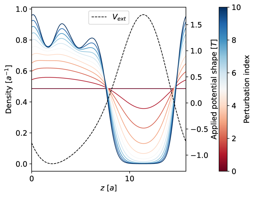
Figure 1: Training data, consisting of the equilibrium densities in a sequence of perturbating potentials with the same shape (dashed line) and increasing amplitude (color scale), shown here for the hard-rod fluid. The densities change from the bulk value at zero potential to a strongly inhomogeneous profile with density approaching zero in the repulsive regions of the potential and saturation with a shell structure in the attractive regions of the potential. We generate 1000 such sets to train and test the ML functional.

Figure 1 shows a sample of the hard-rod fluid training data for one external potential shape. The colored lines show the solutions of the local density profiles over a range of strengths of the external potential, gradually varying from the uniform fluid to a strongly inhomogeneous fluid with different regions approaching zero density and saturation. The minimization of Eq. (11) provides the equilibrium energies $E_{i}$ and densities $n_{i}(r)$, from which we can calculate $F_{i}$ and $\delta F_{i}/\delta n$ for the excess functional. We then use these data to train an ML functional and check how well it can reproduce the results from the known exact functional. (See the SI for an additional exactly-solvable case, the inhomogeneous Ising model in 1D.)

III.2 Hartree-Fock exchange energy

Shifting our attention from classical to electronic DFT, here we consider the much more complex problem of the quantum exchange energy of electrons. Unlike the previous example, there is no analytic density-functional for the exact exchange energy of the Hartree-Fock system. Instead, the exact exchange energy is a non-local functional written in terms of the electronic orbitals $\psi_{i}(\boldsymbol{\mathbf{r}})$,

$$E_{\rm xx}=\frac{-1}{2}\sum_{ij}\iint d\boldsymbol{\mathbf{r}}d\boldsymbol{\mathbf{r}}^{\prime}\psi^{*}_{i}(\boldsymbol{\mathbf{r}})\psi_{j}(\boldsymbol{\mathbf{r}})\psi_{i}(\boldsymbol{\mathbf{r}}^{\prime})\psi^{*}_{j}(\boldsymbol{\mathbf{r}}^{\prime})v_{\rm c}(\boldsymbol{\mathbf{r}}-\boldsymbol{\mathbf{r}}^{\prime}),$$ (13)

where $v_{\rm c}$ is the Coulomb kernel. Note that in 1D, the Coulomb kernel must be regularized at short length scales to avoid a divergence and we use $v_{c}(z)=1/\sqrt{z^{2}+a^{2}}$ as proposed in previous studies of electronic exchange and correlation in 1D.[32]

The total energy of this Hartree-Fock system is calculated in a DFT framework using

$$E=T_{S}[\{\psi_{i}\}]+E_{\rm xx}[\{\psi_{i}\}]+E_{H}[n]+\int d\boldsymbol{\mathbf{r}}V(\boldsymbol{\mathbf{r}})n(\boldsymbol{\mathbf{r}}),$$ (14)

where $T_{S}$ and $E_{\textrm{H}}$ are the kinetic energy and mean-field Coulomb (Hartree) terms as discussed above. While the external and Hartree energies are explicit functionals of the electron density $n(\boldsymbol{\mathbf{r}})$, the kinetic and exchange energies are orbital dependent.

Despite the orbital dependence of the above energy functional, one can still identify an effective local potential for a Kohn-Sham system

$$\left(-\frac{\nabla^{2}}{2}+V_{\textrm{eff}}(\boldsymbol{\mathbf{r}})\right)\psi_{i}(\boldsymbol{\mathbf{r}})=\epsilon_{i}\psi_{i}(\boldsymbol{\mathbf{r}})$$ (15)

that yields the exact solutions for the ground state energy and density $n(\boldsymbol{\mathbf{r}})=\sum_{i}|\psi_{i}(\boldsymbol{\mathbf{r}})|^{2}$ by applying the optimized effective potential (OEP) method.[33] Instead of the usual Kohn-Sham variational equations formulated for explicit density-functionals, the more general OEP method provides an analogous approach for orbital-dependent functionals. We solve for the effective local potential $V_{\textrm{eff}}(\boldsymbol{\mathbf{r}})$ by invoking the variational principle and minimizing the total energy with respect to variations in the potential such that $\delta E/\delta V_{\textrm{eff}}(\boldsymbol{\mathbf{r}})=0$, with the functional derivative of $E[\psi[V]]$ evaluated exactly using automatic differentiation in PyTorch, instead of the conventional perturbation theory approach.[34]

We generate training data for the Hartree-Fock exchange functional in smooth random periodic external potentials, as was done in the case of the hard-rod fluid. In addition, we supplement the training data with random molecules, generated by sampling different numbers of atomic nuclei of various charges to be placed at various separations. Note that the nuclear potentials also use the regularized Coulomb kernel $v_{c}(z)=1/\sqrt{z^{2}+a^{2}}$, consistent with the Hartree and exchange terms, and we set $a=1$ bohr for all our tests. For each case, we use the equilibrium density $n(\boldsymbol{\mathbf{r}})$, the exchange energy $E_{\rm xx}$ and its functional derivative, obtained from the OEP potential as

$$\frac{\delta E_{\rm xx}}{\delta n(\boldsymbol{\mathbf{r}})}=V_{\rm eff}(\boldsymbol{\mathbf{r}})-V(\boldsymbol{\mathbf{r}})-\frac{\delta E_{\textrm{H}}}{\delta n(\boldsymbol{\mathbf{r}})},$$ (16)

for both the training and testing datasets.

III.3 Kohn-Sham kinetic energy

We also test the universal ML density functional for the Kohn-Sham kinetic energy $T_{S}[n]$, which has been attempted previously with specialized approaches.[3, 4] Since the exact kinetic energy of the non-interacting Kohn-Sham system is orbital-dependent,

$$T[\{\psi_{i}\}]=-\frac{1}{2}\sum_{i}\langle\psi_{i}|\nabla^{2}|\psi_{i}\rangle.$$ (17)

we use the OEP approach to construct the density-based training data. Specifically, we solve Eq. (15) in various external potentials $V(\boldsymbol{\mathbf{r}})=V_{\rm eff}(\boldsymbol{\mathbf{r}})$ by directly diagonalizing the Hamiltonian in the plane-wave basis for several $k$-points and compute the corresponding electron density $n(\boldsymbol{\mathbf{r}})$. We then calculate the kinetic energy $T_{s}$ and its functional derivative $\delta T_{s}/\delta n=\mu-V$ from the OEP equation. As above, we produce training data for several smooth random period potentials, spanning a range of box sizes, smoothness and perturbation amplitudes.

III.4 Liquid water

Finally, we target a excess free energy functional for liquid water. A key distinction in this case is that the reference data is not generated from an exact energy functional, but from 3D molecular dynamics (MD) simulations. Here, we restrict to 1D inhomogeneity and consider the planar-averaged density in order to test the universal functional on the same footing as the 1D problems considered above.

We use the mdext extension[35] to LAMMPS[36] to perform MD simulations of water with the SPC/E interatomic potential[37] in the presence of external potentials. We use a $30\times 30\times 40$ Å  box with $\sim 1200$ water molecules in the NVT ensemble at $T=300$ K, equilibrated for 50 ps and collected for 100 ps at each potential strength. In this case, we do not use the random periodic potential because of a challenge in the MD simulations: a potential with multiple minima could lead to trapping of molecules as the strength of the potential increases, with exponential slowdown of the exchange of molecules between the multiple wells formed. To circumvent this MD equilibration issue, we use a potential with shape

$$V(z)=e^{-z^{2}/2\sigma^{2}}(1+Bz^{2})\begin{cases}1,&B<0\\ \pm 1,&0\leq B\leq 0.5\\ -1,&B>0.5\end{cases},$$ (18)

with randomly selected $B$ and $\sigma$. The sign ensures that the potential produces at most one minimum (for $z>0$) and avoids the multiple well problem. (This could lead to two symmetric wells in the MD simulation, but they will end up with nearly the same number of molecules when the trapping occurs, which is the correct equilibrium condition.)

We perform a sequence of simulations with increasing strength of the potential $\lambda V(z)$ applied to the O atoms and collect the density $n_{\lambda}(z)$ of the O atoms of water. This sequence is now a necessity to calculate the free energy of water by thermodynamic integration,

$$A_{\lambda}=\Omega a_{0}+\int_{\lambda^{\prime}=0}^{\lambda}d\lambda\int dzV(z)n_{\lambda}(z),$$ (19)

where $a_{0}$ is the bulk free energy density of the liquid. The corresponding functional derivative $\delta A_{\lambda}/\delta n(z)=-\lambda V(z)$ by the Euler Lagrange equation. Finally, we subtract the total ideal gas free energy in the external potential, $\int dz\,n(T(\log n-1)+\lambda V-\mu)$, and its corresponding functional derivative contribution, to generate the $F$ and $\delta F/\delta n$ required for training the excess functional.

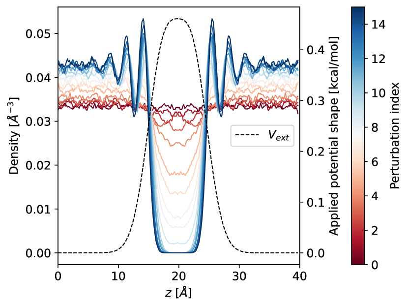
Figure 2: Similar to Figure 1 but for liquid water simulated using SPC/E molecular dynamics simulations instead. The simulations are 3D with a 1D inhomogeneity, and the density shown is planarly-averaged. With increasing potential strength, the water transitions from a uniform density to a strongly inhomogeneous profile ranging from complete exclusion of the density to an oscillating shell structure in the high-density region.

Figure 2 shows the resulting sequence of (planarly-averaged) density profiles of liquid water from the MD simulations for one external potential shape. As the strength of the potential increases, the water is excluded from the repulsive region of the potential and develops an oscillating shell structure with increasing magnitude in the attractive regions of the potential. Note that the density is noisy because the results are derived from histogramming MD trajectories as opposed to evaluating a functional: an additional challenge for the ML functional is to train despite this noise.

IV Results & Discussion

IV.1 Hard-rod fluid

Because an analytic density functional for the hard-rod fluid exists, this example primarily acts as a proof-of-concept to validate our approach. After training the ML models until the test loss in energy and potential stop decreasing, we additionally test the models by solving the Euler-Lagrange equation in several external potentials. This is a more stringent test than the model’s test loss, as the variational optimization can find any instabilities in the functional, such as non-positive-definiteness for specific density profiles, and exploit them to make the energy $\to-\infty$.

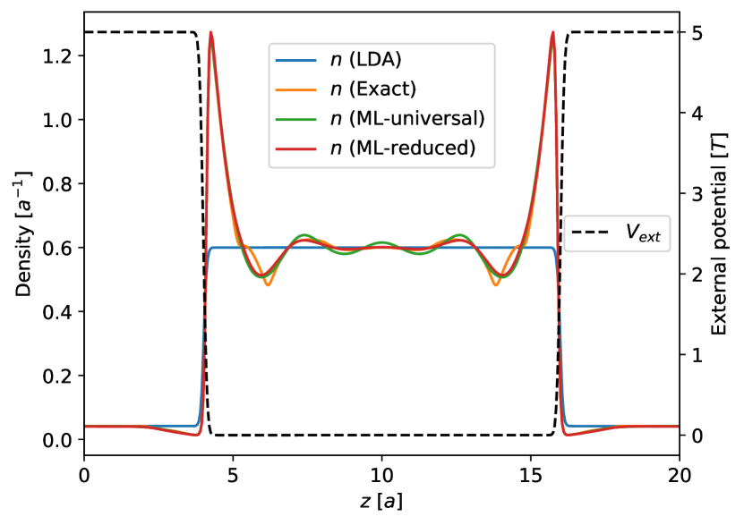
Figure 3: Density profiles for the hard-rod fluid confined to an external potential (dashed line) obtained by solving th Euler-Lagrange equation, compared between the exact functional (Eq. (11)), its local-density approximation and two ML models. The LDA is qualitatively incorrect, while both ML models compare excellently to the exact functional, even with highly reduced model size.

Figure 3 shows the density profiles for the hard-rod fluid in a confining potential compared between the local density approximation (LDA), the exact functional, and two ML models, the universal ML model described in Sec. II.1.4, and a highly reduced ML model with a single convolution layer with 10 even weight functions. (We discuss hyperparameter selection in more detail with our first non-trivial example in the next section for the electronic exchange energy.) Note that the results for the hard-rod fluid are extremely insensitive to the hyperparameters of the ML model. The density profiles from both ML functionals are in excellent agreement with the exact solution, apart from a smoothing out of the density profiles: the exact functional effectively has a sharp step function as a weight function, which cannot be exactly reproduced by the smooth reciprocal space weight functions of our ML models. (The physical cases we care about have smooth interactions anyway, unlike the idealized hard-rod model.) In contrast, the LDA result is qualitatively wrong as it misses the shell structure of the fluid entirely. The performance of the reduced ML model is comparable to our universal ML model, despite having significantly fewer parameters, demonstrating that the even modestly sized ML models suffice for the simple case of the hard-rod fluid.

IV.2 Hartree-Fock exchange energy

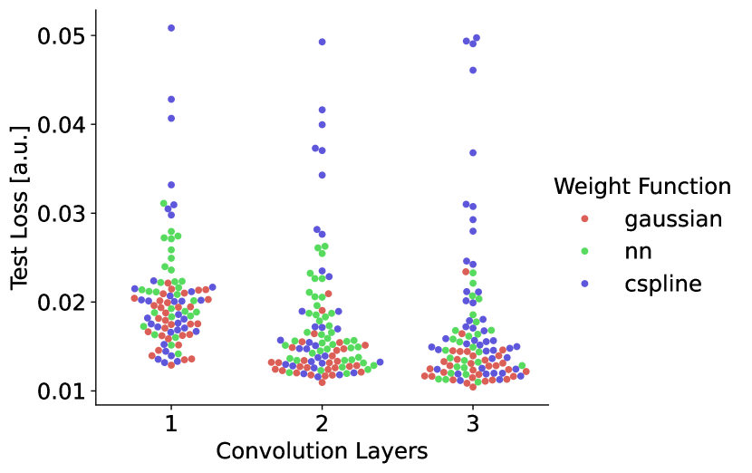
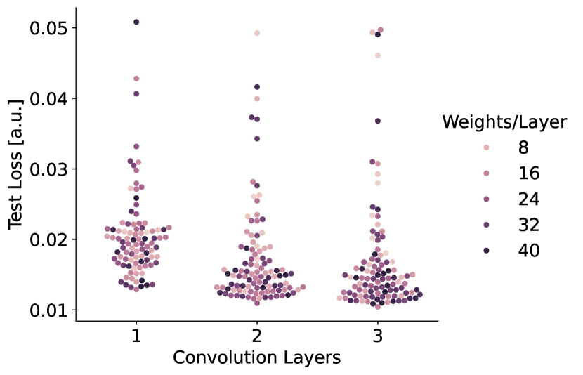
Figure 4: Test loss for Hartree-Fock exchange (energy and potential) as a function of the number of convolution layers colored by (top) type of weight function and (bottom) number of weight functions per layer. Each point corresponds to a randomly selected set of hyperparameters in the ML model.

Our first non-trivial example system examines the exact exchange energy of a Hartree-Fock system of electrons in 1D. We first examined the model performance by varying all hyperparameters of the model, including the number of readout layers, the number of neurons per readout layer, the number of convolution layers, the number of weight functions per convolution layer, weight function type, and the specific hyperparameters within each weight function type (such as $\sigma$ and degree $d$ for the Gaussian weight functions from Eq. (7)). We conducted a random search over all combinations of these parameters and trained 300 separate models to the same data (using the same 80-20 train-test split). Figure 4 shows that the ML model performance is strongly influenced by the number of convolution layers and the type of weight function applied in the ML model. In particular, the accuracy of the model improves a considerable amount increasing from one to two convolution layers and a marginal amount from two to three convolution layers.

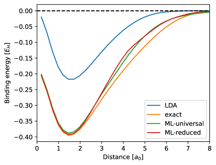
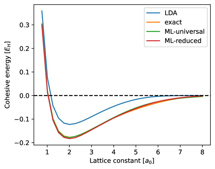
Figure 5: Binding energies of a 1D ‘hydrogen’ molecule (top) and cohesive energies of a infinite hydrogen chain (bottom) as a function of atom separation, predicted by Hartree-Fock theory compared to LDA and two ML models of exchange. LDA underestimates the binding energies, while both ML models, including one with a reduced size, agree remarkably well with the exact results.

Of the three weight function types implemented for this analysis, the Gaussian weight functions perform the best and $\sim 20$ weight functions appear to be sufficient. For hyperparameters specific to Gaussian weights, the best performing models are obtained with polynomials of degree one (see Eq. (7)). Other findings from this hyperparameter search show evidence of 2–3 readout layers with $\sim 30$ neurons per readout layer to be sufficient. We point out the only most noteworthy results of the hyperparameter search here; see the SI for further details and conclusions of this search. Based on this search, we train a ‘reduced’ model consisting of three convolution layers each with only eight Gaussian weight functions of degree 2, and with only two readout layers of 90 neurons each, in addition to the universal hyperparameters from Sec. II.1.4.

To test the functional for its intended application, energy differences and electronic structure of atomic configurations, we investigate the binding energy of an isolated hydrogen molecule and the cohesive energy of a periodic chain of hydrogen atoms, both computed as the difference in energy from an isolated hydrogen atom. Note that this 1D atomic ‘hydrogen’ here refers to a species having a nuclear charge of $Z=1$, with a potential based on the regularized 1D Coulomb interaction, and is fundamentally distinct from the actual element hydrogen. Figure 5 shows that the LDA strongly underestimates the binding and cohesive energies in both cases, which is different from the 3D case as a result of the short-range cutoff in the 1D Coulomb kernel that is not present in the 3D kernel. Both ML functionals agree remarkably well with the exact solution for both the binding and cohesive energies. Furthermore the reduced model performs comparably to the universal model, suggesting that the cost of the ML model may be reduced without sacrificing the accuracy of the calculation.

IV.3 Kohn-Sham kinetic energy

The strongly nonlocal nature of the Kohn-Sham kinetic energy makes this functional challenging to train, which we test in a randomized hyperparameter scan of 300 ML models (see SI). The hyperparameter search reveals the performance of this functional to be highly sensitive to the choice of hyperparameters, especially compared to the Hartree-Fock exchange energy and the hard-rod fluid. In particular, we find lower test errors from the ML models which have more trainable parameters, including both the number of weight functions and convolution layers (see Supplemental Information for a more detailed discussion). Accordingly, we test the (larger) optimal model from this hyperparameter scan along with the universal model. The optimal model from the scan (i.e. lowest test errors) consists of two convolution layers with 62 total weight functions each, three readout layers of 90 neurons each, and Gaussian-polynomial weight functions with $d=2$.

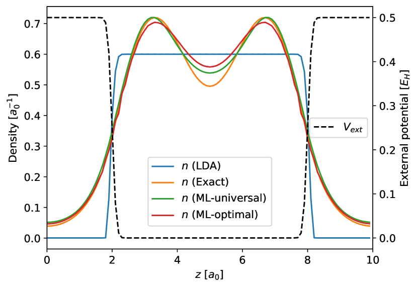
Figure 6: Density profiles for non-interacting electrons confined to an external potential shown by the dashed line, predicted by orbital-free kinetic energy functionals at the LDA level and with two ML models, compared to the exact orbital-dependent calculation. While the LDA result is qualitatively incorrect, the ML models are in reasonable agreement with the exact solution, capturing the tunneling and Friedel oscillations in the high and low regions respectively of the potential (dashed line).

Figure 6 shows the resulting density profiles for the Kohn-Sham system in a periodic rectangular well. The density profiles from both the universal and optimal ML models agree well with the exact solution, while the Thomas-Fermi LDA result yields results that are qualitatively incorrect. Most impressively, the ML models capture the exponential decay of the electron density in the classically-forbidden tunneling region, as well as the Friedel oscillations in the electron density in the allowed region, all from an orbital-free DFT with no Schrödinger equation solution. Also note that this potential well is qualitatively different from the random periodic potentials in the training set, indicating that our universal ML model is able to generalize well to physically-distinct environments.

IV.4 Liquid water

Finally, we test the classical DFT for a real fluid, liquid water, with 1D inhomogeneity. With a hyperparameter scan of 300 random ML models, we determine the optimal set of parameters for water by training to the SPC/E water data described in Sec. III.4. We find the optimal model parameters to have three convolution layers with 18 Gaussian weights each and two readout layers with 80 neurons each, which is notably smaller than our universal model.

We test the reduced and universal ML models as excess functionals for classical DFT and solve the Euler-Lagrange equation with two external potential shapes, a square wave and a sine wave, both distinct from those included within our ML training and testing datasets. Figure 7 shows that both the optimal and universal ML models successfully reproduce the density profiles from the MD simulations, apart from small quantitative differences which are notably comparable to the magnitude of noise in the MD density. The density profiles from the LDA, however, are qualitatively incorrect as they miss the oscillations of the density entirely. These results demonstrate that the universal ML functional is capable of extrapolating very well to potentials with abruptly and slowly-varying shapes that are qualitatively distinct from the the training data. Additionally, the universal ML model predicts the free energy with errors of 0.04 and $<$0.01 kcal/mol/Ų respectively for the square and sine wave cases, compared to 0.1 and 0.2 kcal/mol/Ų respectively for LDA, showing that the ML classical DFTs are capable of achieving chemical accuracy for solvation.

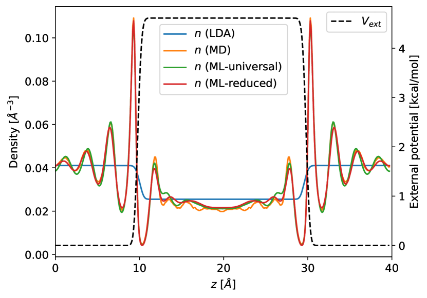
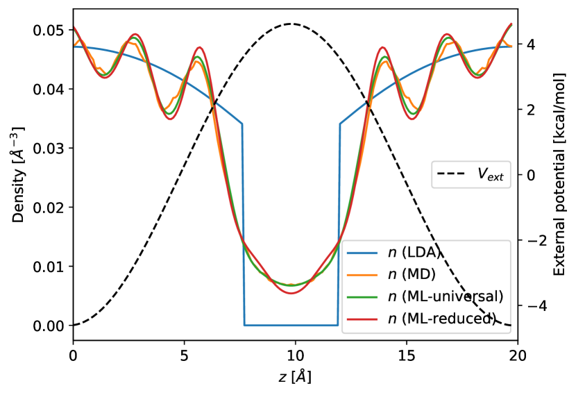
Figure 7: Density profiles of liquid water from SPC/E molecular dynamics compared to LDA and two ML functionals for external potential shapes (dashed lines) completely distinct from those in the training and testing datasets. LDA is qualitatively inadequate as an excess functional, while both ML functionals quantitatively reproduce the non-trivial density profiles with shell structure, in both the square and sine-wave potentials.

IV.5 Summary

Once trained, a single universal ML model performs remarkably well across four physically distinct problems spanning classical and electronic DFT. In comparison to the universal ML model, hyperparameter searches for single-task ML models reveal that significantly smaller ML models are sufficient for all but one case: the Kohn-Sham kinetic energy, which we find to be the most challenging functional to learn. The ML functionals effectively reproduce the exact results in each case, whereas the LDA is qualitative incorrect in all but the exchange energy case, where it is only quantitatively incorrect, as the orbital-dependent kinetic energy regulates the system to produce qualitatively correct behavior.

These results confirm that ML functionals have the potential to substantially improve functional approximations for DFT—for both classical and electronic theories—and expand the scope of DFT to highly non-trivial cases requiring nonlocal functionals. Hence, ML functionals can expand DFT significantly beyond Kohn-Sham electronic DFT, where only the exchange-correlation functional is approximated and where semi-local approximations have been reasonably successful. Moreover, these same ML functionals can considerably accelerate the usability of classical DFT, where semi-local approximations have been shown to be grossly inadequate, to help overcome the bottleneck of developing classical density functionals.

V Conclusions

We have formulated a general ML functional approximation framework that combines the best features from equivariant convolutional neural networks and the weighted-density approximation. Our approach includes a general protocol for generating data and for training such functionals, which we go on to apply to fundamentally distinct systems. We systematically tested hundreds of ML models having random combinations of weight function parameterizations, convolution layers, activation functions and readout functions to identify a set of hyperparameters that work for widely-different density functional theories. We demonstrated that we can build a universal ML model, that is trained to data from these distinct physical systems but uses exactly the same hyperparameters, that performs remarkably well and reproduces highly non-trivial features in the density profiles and energies that are missed completely by semi-local approximations. In particular, we showed that in addition to exactly solvable models, the ML functional performs excellently for the exact exchange energy and kinetic energy of electrons in 1D, as well as for the excess functional of (3D) liquid water with 1D inhomogeneity. Remarkably, these functionals show promise of achieving useful orbital-free electronic DFT as well as classical DFT of liquid water with chemical accuracy for solvation.

Here, we prototyped all models in 1D in order to rapidly generate data for several physically-distinct systems and test the universality of the ML approach. While we lay out the extension to 3D for the ML functional approach already, the cost of generating high quality data to train the functionals can become the bottleneck, e.g., OEP calculations for exchange in 3D are very expensive, and collecting 3D density profiles from MD will require much longer collection times due to increased statistical errors; these extensions may require further methodological developments beyond brute-force large-scale computation. Finally, for the classical DFT case, this framework can eliminate the need for classical interatomic potentials altogether by applying ML interatomic potentials trained to ab initio molecular dynamics (AIMD) of inhomogeneous fluids,[35] directly constraining classical DFT to AIMD for truly ab initio solvation models.

References

References

- Burke [2012] K. Burke, J. Chem. Phys. 136, 150901 (2012).
- Perdew [2013] J. P. Perdew, MRS Bullet. 38, 743–750 (2013).
- Snyder et al. [2012] J. C. Snyder, M. Rupp, K. Hansen, K.-R. Müller, and K. Burke, Phys. Rev. Lett. 108, 253002 (2012).
- Brockherde et al. [2017] F. Brockherde, L. Vogt, L. Li, M. Tuckerman, K. Burke, and K. Müller, Nature Commun. 8 (2017), 10.1038/s41467-017-00839-3.
- Mermin [1965] N. D. Mermin, Phys. Rev. 137, A1441 (1965).
- Capitani et al. [1982] J. F. Capitani, R. F. Nalewajski, and R. G. Parr, J. Chem. Phys. 76, 568 (1982).
- Petrosyan et al. [2007] S. A. Petrosyan, J.-F. Briere, D. Roundy, and T. A. Arias, Phys. Rev. B 75, 205105 (2007).
- Curtin and Ashcroft [1985] W. A. Curtin and N. W. Ashcroft, Phys. Rev. A 32, 2909 (1985).
- Percus [1988] J. K. Percus, J. Stat. Phys. 52, 1157 (1988).
- Roth [2010] R. Roth, J. Phys.: Cond. Matt. 22, 063102 (2010).
- Zhao et al. [2011] S. Zhao, Z. Jin, and J. Wu, J. Phys. Chem. B 115, 6971 (2011).
- Yu and Wu [2002] Y.-X. Yu and J. Wu, J. Chem. Phys. 117, 2368 (2002).
- Sundararaman et al. [2012] R. Sundararaman, K. Letchworth-Weaver, and T. A. Arias, J . Chem. Phys. 137, 044107 (2012).
- Sundararaman and Arias [2014] R. Sundararaman and T. Arias, Comp. Phys. Comm. 185, 818 (2014).
- Sundararaman et al. [2014] R. Sundararaman, K. Letchworth-Weaver, and T. Arias, Journal of Chemical Physics 140, 144504 (2014).
- Wu and Gu [2023] J. Wu and M. Gu, The Journal of Physical Chemistry Letters 14, 10545 (2023).
- Grisafi et al. [2019] A. Grisafi, A. Fabrizio, B. Meyer, D. M. Wilkins, C. Corminboeuf, and M. Ceriotti, ACS Central Science 5, 57 (2019), pMID: 30693325, https://doi.org/10.1021/acscentsci.8b00551 .
- Nigam et al. [2022] J. Nigam, M. J. Willatt, and M. Ceriotti, The Journal of Chemical Physics 156, 014115 (2022), https://pubs.aip.org/aip/jcp/article-pdf/doi/10.1063/5.0072784/16533109/014115_1_online.pdf .
- Unke et al. [2021] O. T. Unke, M. Bogojeski, M. Gastegger, M. Geiger, T. Smidt, and K. R. Muller, in Advances in Neural Information Processing Systems, edited by A. Beygelzimer, Y. Dauphin, P. Liang, and J. W. Vaughan (2021).
- Zhong et al. [2024] Y. Zhong, H. Yu, J. Yang, X. Guo, H. Xiang, and X. Gong, “Universal machine learning kohn-sham hamiltonian for materials,” (2024), arXiv:2402.09251.
- Li et al. [2022] H. Li, Z. Wang, N. Zou, M. Ye, R. Xu, X. Gong, W. Duan, and Y. Xu, Nat Comput Sci 2, 367 (2022).
- Gong et al. [2023] X. Gong, H. Li, N. Zou, R. Xu, W. Duan, and Y. Xu, Nat Commun 14, 2848 (2023).
- Mardirossian and Head-Gordon [2016] N. Mardirossian and M. Head-Gordon, The Journal of Chemical Physics 144, 214110 (2016).
- Dick and Fernandez-Serra [2020] S. Dick and M. Fernandez-Serra, Nature Commun. 11, 3509 (2020).
- Bystrom and Kozinsky [2023] K. Bystrom and B. Kozinsky, “Nonlocal Machine-Learned Exchange Functional for Molecules and Solids,” (2023), arXiv:2303.00682.
- del Mazo-Sevillano and Hermann [2023] P. del Mazo-Sevillano and J. Hermann, “Variational principle to regularize machine-learned density functionals: The non-interacting kinetic-energy functional,” (2023), arXiv:2306.17587.
- Hohenberg and Kohn [1964] P. Hohenberg and W. Kohn, Phys. Rev. 136, B864 (1964).
- Kohn and Sham [1965] W. Kohn and L. Sham, Phys. Rev. 140, A1133 (1965).
- Percus [1976] J. K. Percus, Journal of Statistical Physics 15, 505 (1976).
- Vanderlick et al. [1989] T. K. Vanderlick, H. T. Davis, and J. K. Percus, The Journal of Chemical Physics 91, 7136 (1989), https://pubs.aip.org/aip/jcp/article-pdf/91/11/7136/18984050/7136_1_online.pdf .
- Percus [1982] J. K. Percus, Journal of Statistical Physics 28, 67 (1982).
- Helbig et al. [2011] N. Helbig, J. I. Fuks, M. Casula, M. J. Verstraete, M. A. L. Marques, I. V. Tokatly, and A. Rubio, Phys. Rev. A 83, 032503 (2011).
- Wu and Yang [2003] Q. Wu and W. Yang, The Journal of Chemical Physics 118, 2498 (2003), https://pubs.aip.org/aip/jcp/article-pdf/118/6/2498/19133218/2498_1_online.pdf .
- Krieger et al. [1992] J. B. Krieger, Y. Li, and G. J. Iafrate, Phys. Rev. A 46, 5453 (1992).
- Fazel et al. [2024] K. Fazel, N. Karimitari, T. Shah, C. Sutton, and R. Sundararaman, J. Comput. Chem. , in press (2024), dOI: 10.1002/jcc.27353.
- Plimpton [1995] S. Plimpton, J. Comput. Phys. 117, 1 (1995).
- Berendsen et al. [1987] H. J. C. Berendsen, J. R. Grigera, and T. P. Straatsma, J. Phys. Chem. 91, 6269 (1987).