Beyond spin-charge separation: Helical modes and topological quantum phase transitions in one-dimensional Fermi gases with spin-orbit and Rabi couplings

Abstract

Motivated by the experimental observation of spin-charge separation in one-dimensional interacting Fermi gases, we investigate these systems in the presence of spin-orbit coupling and Rabi fields. We demonstrate that spin-charge-separated modes evolve into helical collective modes due to the special mixing of spin and charge induced by spin-orbit coupling and Rabi fields. We obtain the phase diagram of chemical potential versus Rabi fields for given spin-orbit coupling and interactions, and find several topological quantum phase transitions of the Lifshitz type. We show that the velocities of the collective modes are nonanalytic at the boundaries between different phases. Lastly, we analyze the charge-charge, spin-charge and spin-spin dynamical structure factors to show that the dispersions, spectral weights and helicities of the collective modes can be experimentally extracted in systems such as ${}^{6}{\rm Li}$, ${}^{40}{\rm K}$ and ${}^{173}{\rm Yb}$.

Introduction: While spin and charge are intrinsic properties of elementary particles, in one dimension (1D), interactions are responsible for the separation of spin and charge leading to spin-density (SDW) and charge-density (CDW) waves that propagate with different velocities. Spin-charge separation is theoretically described by the Tomonaga-Luttinger liquid model [1, 2, 3, 4, 5, 6] in condensed matter physics (CMP), but is regarded as a general phenomenon of a large variety of quantum fields: non-Abelian Yang-Mills theory describing knotted strings as stable solitons [7, 8, 9], supersymmetric gauge theory characterizing magnetic superconductors [10], and quark-lepton unification theory suggesting the similarity between spinons and neutrinos [11]. A few experiments in condensed matter have claimed observing spin-charge separation: angle-resolved photoemission in $\text{SrCuO}_{2}$ [12, 13] and tunneling spectroscopy in GaAs/AlGaAs heterostructures [14, 15] at low temperatures. Very recently, spin-charge separation was also observed in ultracold gases (${}^{6}\text{Li}$) as a function of interactions and temperature [16, 17]. A major experimental advantage of ultracold gases over condensed matter and high energy systems is the tunability of interactions, temperature, density and external fields, permitting for a thorough exploration of spin-charge separation and mixing [16, 17]. This tunability allows for investigations of the interplay between spin and charge degrees of freedom in unprecedented ways like, for instance, as a function of synthetic spin-orbit coupling, Rabi (spin-flip) fields, density or chemical potential.

In CMP, spin-orbit coupling (SOC) is a relativistic quantum mechanical effect that entangles the spin of a particle to its spatial degrees of freedom. SOC plays an important role in spin-Hall systems  [18, 19] and topological insulators [20, 21] and superconductors [22, 23, 24]. However, tunability of SOC, spin-flip fields, density or chemical potential is limited. There are two common types of SOC: the Rashba [25] and the Dresselhaus [26] terms, that have been discussed in the context of semiconductors [27, 28, 29, 30, 31, 32]. In ultracold atoms, SOC is synthetically created using two-photon Raman transitions instead of originating from relativistic effects [33, 34]. This makes SOC tunable in bosonic [35, 36, 37] and fermionic [38, 39, 40] quantum gases, where equal mixtures of Rashba and Dresselhaus (ERD) terms have been created [35], as well as, Rashba-only (RO) [41, 42, 43]. Furthermore, Dresselhaus-only (DO) and arbitrary mixtures of Rashba and Dresselhaus terms have also been suggested [44].

Inspired by the observation of spin-charge separation in 1D interacting Fermi gases [16], we explore the effects of SOC and Rabi fields on spin-charge separation and show that spin and charge density modes evolve into spin-charge-mixed helical collective modes. We investigate the phase diagram of chemical potential versus Rabi fields for given SOC and interactions, revealing several topological quantum phase transitions of the Lifshitz type. We demonstrate that the velocities of the helical collective modes are nonanalytic at the boundaries between different phases, and show that the charge-charge, spin-charge and spin-spin dynamical structure factors [16, 17, 45, 46] reveal the dispersions, spectral weights and helicities of the collective modes in experimentally accessible systems such as ${}^{6}{\rm Li}$, ${}^{40}{\rm K}$ and ${}^{173}{\rm Yb}$.

Hamiltonian: To describe the rich SOC physics outlined above, we consider the experimentally realized kinetic energy operator [35]

$${\hat{K}}=\epsilon_{k}I-h_{x}\sigma_{x}-h_{z}(k)\sigma_{z},$$ (1)

where $k$ is the momentum along the $x$ direction, $\epsilon_{k}={(k^{2}+k_{T}^{2})}/{2m}$ is the shifted kinetic energy, $k_{T}$ is the spin-dependent momentum shift, $h_{x}$ is the Rabi field, and $h_{z}(k)={kk_{T}}/{m}$ is the SOC. We diagonalize ${\hat{K}}$ using a momentum-dependent ${\rm SU(2)}$ rotation $U(k)$ to obtain the eigenvalues $E_{A}(k)=\epsilon_{k}-h_{\text{eff}}(k)$ and $E_{B}(k)=\epsilon_{k}+h_{\text{eff}}(k)$, where $h_{\text{eff}}(k)=\sqrt{h_{x}^{2}+h_{z}^{2}(k)}$.

In Fig. 1, $E_{A}(k)$ and $E_{B}(k)$ are shown for various situations. When $h_{x}\neq 0$, $E_{A}(k)$ and $E_{B}(k)$ are non-degenerate with $E_{A}(k)$ having either double minima $(|h_{x}|<2E_{T})$, shown in Fig. 1(a,c,e,g), or a single minimum $(|h_{x}|\geq 2E_{T})$ seen in Fig. 1(b,d,h), where $E_{T}=k_{T}^{2}/2m$. When $h_{x}=0$, we have $h_{\text{eff}}(k)=|h_{z}(k)|$ and the two bands intersect at $k=0$, as shown in Fig. 1(f). The creation operators for the energy basis are $(a_{k,A}^{\dagger}\ a_{k,B}^{\dagger})=(c_{k,\uparrow}^{\dagger}\ c_{k,\downarrow}^{\dagger})U^{\dagger}(k)$, where $c^{\dagger}_{k,s}$ are the creation operators with momentum $k$ and spin $s=\{\uparrow,\downarrow\}$. The operators $a^{\dagger}_{\alpha}$ create helical fermions, because the matrix $U(k)$ has an ${\rm SU(2)}$ momentum-dependent rotation angle $\theta(k_{T},h_{x},k)$, when both $k_{T}$ and $h_{x}$ are non-zero.

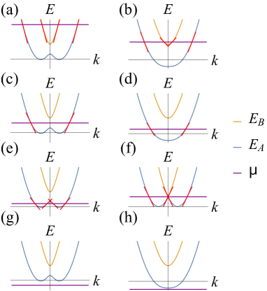
Figure 1: Schematic plots of $E_{A}(k)$ (blue solid line) and $E_{B}(k)$ (orange solid line) showing effects of SOC $(k_{T})$ and Rabi fields $(h_{x})$. The red solid lines are linearizations around Fermi points, and the horizontal purple solid lines indicate $\mu$. In panels (a), (c), (e) and (g), $E_{A}(k)$ has double minima, since $|h_{x}|/E_{T}<2$. In panels (b), (d), and (h), $E_{A}(k)$ has a single minimum, since $|h_{x}|/E_{T}\geq 2$. In panel (f), $h_{x}=0$, and the system is equivalent to no SOC due to the spin-gauge symmetry.

Interactions for two-internal-state ${}^{6}{\rm Li}$, ${}^{40}{\rm K}$ or ${}^{173}{\rm Yb}$ are ${\hat{V}}=V_{0}\int_{0}^{L}\differential x^{\prime}\int_{0}^{L}\differential x{\hat{n}}_{\uparrow}(x){\hat{n}}_{\downarrow}(x^{\prime})f(|x-x^{\prime}|),$ where ${\hat{n}}_{s}(x)=\psi_{s}^{\dagger}(x)\psi_{s}(x)$ is the local density operator with $s=\{\uparrow,\downarrow\}$ and $L$ is the length of system. The parameter $V_{0}$, with dimensions of energy, controls the strength and the dimensionless function $f(|x-x^{\prime}|)$ controls the range $r_{0}$ of the interaction. In momentum space

$${\hat{V}}=\frac{V_{0}}{L}\sum_{q}{\hat{\rho}}_{\uparrow}(q){\hat{\rho}}_{\downarrow}(-q){\tilde{f}}(q),$$ (2)

where ${\hat{\rho}}_{s}(q)=\sum_{k}c^{\dagger}_{k+q,s}c_{k,s}$ is the Fourier transform of the local density operator ${\hat{n}}_{s}(x)$, and ${\tilde{f}}(q)=\int d\eta e^{-{\rm i}q\eta}f(|\eta|)$ is the Fourier transform of $f(|x-x^{\prime}|)$ with dimensions of length. When $h_{x}=0$, the spin-gauge transformation $\psi_{\uparrow}(x)\rightarrow e^{{\rm i}k_{T}x}\psi_{\uparrow}(x),\ \psi_{\downarrow}(x)\rightarrow e^{-{\rm i}k_{T}x}\psi_{\downarrow}(x)$ gauges away $k_{T}$ in the kinetic energy without changing the interaction ${\hat{V}}$ (spin-gauge symmetry).

Bosonization: To describe the low-energy excitations, we use the bosonization technique. We approximate ${\hat{K}}$ in Eq. (1) by linearizing it around the chemical potential $\mu$. There are four general cases shown in Fig. 1: (I) $\mu$ intersects twice $E_{A}(k)$ and twice $E_{B}(k)$, see Figs. 1(a,b); (II) $\mu$ intersects only band $E_{A}(k)$ twice, see Figs. 1(c,d); (III) $\mu$ intersects $E_{A}(k)$ four times, see Fig. 1(e); (IV) $\mu$ does not intersect $E_{A}(k)$ or $E_{B}(k)$, see Fig. 1(g,h). Intersection of $\mu$ to either $E_{A}(k)$ or $E_{B}(k)$ allows for linearization of dispersions, shown as red lines in Fig. 1. We label particles by indices $\{r,\alpha\}$: $r$ describes left ($L$) or right ($R$) moving fermions; $\alpha$ labels $A$ or $B$ indicating linearization of $E_{A}(k)$ or $E_{B}(k)$. In the special case of Fig. 1(e), we set $\alpha=A^{(1)}$ for the outer red lines and $\alpha=A^{(2)}$ for the inner red lines, since only $E_{A}(k)$ is crossed by $\mu$. The linearized kinetic energy operator is

$${\hat{K}}=\sum_{k,r,\alpha}u_{\alpha}\big{[}\operatorname{sgn}(r)k-k_{\mu,\alpha}\big{]}a^{\dagger(r)}_{k,\alpha}a^{(r)}_{k,\alpha},$$ (3)

where $u_{\alpha}$ is the Fermi velocity $dE_{\alpha}(k)/dk$ at $k=k_{\mu,\alpha}$, with $k_{\mu,\alpha}$ being the positive momentum where $\mu$ intersects the relevant band. Both $u_{\alpha}$ and $k_{\mu,\alpha}$ depend on $k_{T}$, $h_{x}$ and $\mu$. The function $\operatorname{sgn}(r)$ refers to the sign of $r$, where $\operatorname{sgn}(R)=+1$ and $\operatorname{sgn}(L)=-1$.

We bosonize ${\hat{K}}$ in Eq. (3) using the transformation

$$b_{q,\alpha}^{\dagger}=\sqrt{\frac{2\pi}{|q|L}}\sum_{r}\Theta\big{(}-\operatorname{sgn}(r)q\big{)}{\hat{\rho}}_{\alpha}^{\dagger(r)}(q),$$ (4)

where ${\hat{\rho}}_{\alpha}^{(r)}(q)$ are the fermion density operators, and $\Theta(x)$ is the step function. This leads to ${\hat{K}}=\sum_{q,\alpha}|qu_{\alpha}|b_{q,\alpha}^{\dagger}b_{q,\alpha}$ for the kinetic energy and to

$${\hat{V}}=\frac{V_{0}}{\pi}\sum_{q>0}q{\boldsymbol{\Phi}}^{\dagger}(q){\bf g}{\boldsymbol{\Phi}}(q)$$ (5)

for the interaction, where ${\boldsymbol{\Phi}}(q)$ is either a two-component vector or a four-component vector, and ${\bf g}$ is either a $2\times 2$ or a $4\times 4$ matrix. In case (I), where bands $A$ and $B$ are crossed, ${\boldsymbol{\Phi}}^{T}(q)=\begin{pmatrix}b_{q,A}^{\dagger}&b_{q,B}^{\dagger}&b_{-q,A}&b_{-q,B}\end{pmatrix}.$ In case (II), where band $A$ is crossed at two Fermi points, ${\boldsymbol{\Phi}}^{T}(q)=\begin{pmatrix}b_{q,A}^{\dagger}&b_{-q,A}\end{pmatrix}.$ In case (III), where band $A$ is crossed at four Fermi points, ${\boldsymbol{\Phi}}^{T}(q)=\begin{pmatrix}b_{q,A^{(1})}^{\dagger}&b_{q,A^{(2)}}^{\dagger}&b_{-q,A^{(1)}}&b_{-q,A^{(2)}}\end{pmatrix}.$ The matrix elements of ${\bf g}$ are $g_{ij}=\eta_{ij}{\tilde{f}}(q\to 0)$, having dimensions of length, while $\eta_{ij}$ is dimensionless and depends on $k_{T}$, $h_{x}$ and $\mu$.

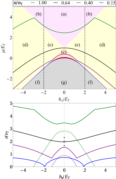
Figure 2: Phase diagram and velocities of collective modes. In panel (a), we show the phase diagram of $\mu/E_{T}$ versus $h_{x}/E_{T}$, where $E_{T}=k_{T}^{2}/2m$ for $V_{0}/E_{T}=2$. The pink, yellow, orange and gray regions represent phases with four (two), two (one), four (two) and zero (zero) Fermi points (collective modes), respectively separated by topological quantum phase (Lifshitz) transitions. In the red region the lower velocity mode is unstable. The vertical black dashed lines at $|h_{x}|/E_{T}=2$ separate regions where $E_{A}(k)$ has single minimum $|h_{x}|/E_{T}<2$ or double minima $|h_{x}|/E_{T}>2$. The letters $a,b,c,e,f,g$ represent the dispersions shown in Fig. 1. The green, black, purple and blue solid lines represent fixed densities $n/n_{T}=\{1.00,0.64,0.40,0.15\}$, respectively. In panel (b), we show the velocities $v/v_{T}$ of collective modes versus $h_{x}/E_{T}$ in green (solid and dashed) for $n_{/}n_{T}=1.00$, in black solid for $n/n_{T}=2/\pi\approx 0.64$, in purple (solid and dashed) for $n_{/}n_{T}=0.40$ and in blue (solid) for $n/n_{T}=0.15$. The velocities are nonanalytic at the boundaries of phases, and the line $h_{x}/E_{T}$ represents the spin-charge separation locus.

Collective modes: The bosonized Hamiltonian ${\hat{H}}={\hat{K}}+{\hat{V}}$ is diagonalized via a Bogoliubov transformation ${\bf B}$ leading to boson operators $\Psi^{T}(q)=\begin{pmatrix}d_{q,1}^{\dagger}&d_{q,2}^{\dagger}&d_{-q,1}&d_{-q,2}\end{pmatrix}$ for cases (I) and (III), where the number of collective modes is $N_{C}=2$ and to $\Psi^{T}(q)=\begin{pmatrix}d_{q,1}^{\dagger}&d_{-q,1}\end{pmatrix}$ for case (II), where $N_{C}=1$. Barring any instabilities, $N_{C}=N_{F}/2$, where $N_{F}$ is the number of Fermi points at $\mu$. The transformation $\Psi(q)={\bf B}\Phi(q)$ leads to the diagonalized Hamiltonian

$${\hat{H}}=\sum_{q,m}|q|v_{m}d_{q,m}^{\dagger}d_{q,m}+\omega_{\Omega},$$ (6)

where $v_{m}\geq 0$ is the velocity of collective mode $m$ that depends on $\{k_{T},h_{x},\mu\}$ for given $V_{0}$. The ground state energy is $\omega_{\Omega}=E_{\Omega}-K_{\Omega}$, where $E_{\Omega}=\sum_{q>0,m}|qv_{m}|$ and $K_{\Omega}=\sum_{q>0,\alpha}|qu_{\alpha}|$.

In Fig. 2(a), we show the phase diagram of $\mu/E_{T}$ versus $h_{x}/k_{T}$, for $V_{0}/E_{T}=2$. In the pink region, $N_{F}=4$ as in Fig. 1(a)-(b) and $N_{C}=2$. In the yellow region, $N_{F}=2$ as in Fig 1(c)-(d) and $N_{C}=1$. In the orange region, $N_{F}=4$ as in Fig. 1(e) and $N_{C}=2$. For the vertex separating the pink, yellow and orange regions ($h_{x}/E_{T}=0$ and $\mu/E_{T}=1$), $N_{F}=4$ as in Fig. 1(f) and $N_{C}=2$; at this location there is perfect spin-charge separation. In fact, along the line $h_{x}/E_{T}=0$, there is spin-charge separation also in the pink and orange regions, due to the spin-gauge symmetry. In the red region, the lower-velocity collective mode becomes unstable. This instability arises from the breakdown of the positive definiteness of the Hamiltonian with respect to the complex symplectic group ${\rm Sp}(4,{\bf C})$ that the Bogoliubov transformation satisfies [47]. In the gray region, $N_{F}=0$ and $N_{C}=0$, since $\mu$ lies below the energy bands as in Fig. 1(g)-(h); this the zero density limit.

Furthermore, in Fig. 2(a), the lines or points separating different phases indicate topological quantum phase transitions of the Lifshitz-type [48], where the Fermi surfaces change from four to two to zero points, depending on $\mu/E_{T}$ and $h_{x}/E_{T}$. The vertical black dashed lines at $h_{x}/E_{T}=\pm 2$ separate regions where the lower band has two minima $(|h_{x}|/E_{T}<2)$ from regions where the lower band has one minimum $(|h_{x}|/E_{T}>2)$ and the line at $h_{x}/E_{T}=0$ represents the locus of spin-charge separation. Since experiments are performed at fixed densities, the solid lines are constant density curves in units of $n_{T}=k_{T}$. The densities are as follows: $n/n_{T}=1.00$ (green line), $n/n_{T}=2/\pi\approx 0.64$ (black line), $n/n_{T}=0.40$ (purple line), $n/n_{T}=0.15$ (red line).

In Fig. 2(b), we show the collective mode velocities $v/v_{T}$ versus $h_{x}/E_{T}$, where $v_{T}=k_{T}/m$, at $V_{0}/E_{T}=2$ for fixed densities $n/n_{T}=1.00$ (green solid and dashes lines), $n/n_{T}=0.64$ (black solid and dashed lines), $n/n_{T}=0.40$ (purple solid and dashed lines), and $n/n_{T}=0.15$ (blue solid line). Notice that $v/v_{T}$ is continuous, but nonanalytic every time a phase boundary is crossed; this behavior is a direct consequence of a topological (Lifshitz) quantum phase transition. There are always two modes in the pink region, one mode in the yellow region, two modes in the orange region, one mode in the red region, and no modes in the gray region. For $h_{x}/E_{T}=0$ there is perfect spin-charge separation, and when two modes exist the higher-velocity mode is associated with charge and the lower-velocity mode is associated with spin. As the density is lowered into the red region of Fig. 2(a), the spin mode becomes unstable, and only the charge mode survives. In the absence of SOC $(k_{T}=0)$ with $h_{x}\neq 0$, the collective modes are generally a mix of charge and spin density waves, but they are nonhelical. However, when both $k_{T}\neq 0$ and $h_{x}\neq 0$, the collective modes are a mix of charge and spin density waves with a helical structure, which is carried over by the momentum-dependent rotation angles $\theta(k_{T},h_{x},k)$ of the ${\rm SU(2)}$ rotation matrices $U(k)$.

To visualize helical modulations, we write $d_{q,m}=\sum_{r}\big{[}A_{m}^{(r)}(q){\hat{\rho}}^{(r)}(q)+{\bf B}_{m}^{(r)}(q)\cdot{\hat{\boldsymbol{\sigma}}}^{(r)}(q)\big{]}$ in terms of the Fourier transforms ${\hat{\rho}}^{(r)}(q)$ and ${\hat{\boldsymbol{\sigma}}}^{(r)}(q)$ of the charge-density ${\hat{n}}^{(r)}(x)=\sum_{s}\psi_{s}^{\dagger(r)}(x)\psi_{s}^{(r)}(x)$ and spin-density ${\hat{\bf S}}^{(r)}(x)=\sum_{ss^{\prime}}\psi_{s}^{\dagger(r)}(x)(\boldsymbol{\sigma})_{ss^{\prime}}\psi_{s^{\prime}}^{(r)}(x)$ operators, respectively. The collective mode operators in real space are ${\cal D}_{m}(x)=\sum_{r}\int\differential x^{\prime}\big{[}a_{m}^{(r)}(x-x^{\prime}){\hat{n}}^{(r)}(x^{\prime})+{\bf b}_{m}^{(r)}(x-x^{\prime})\cdot{\hat{\bf S}}^{(r)}(x^{\prime})\big{]},$ where the spatial modulation and helicity of the vector fields ${\bf b}_{m}^{(r)}(x-x^{\prime})$ are controlled by $k_{T}$ and $h_{x}$. When $k_{T}$ and $h_{x}$ are both non-zero, all the modes present are helical, with $q>0$ $(q<0)$ modes having positive (negative) helicity. The global helicity of the Hamiltonian in Eq. (6) is zero, such that $q>0$ and $q<0$ bosons for each mode are helical pairs.

For ${}^{6}{\rm Li}$, ${}^{40}{\rm K}$, and ${}^{173}\rm{Yb}$ typical SOC and Rabi fields are known [38, 49, 50]. Optical boxes in 1D have typical dimensions from $10\mu{\rm m}$ to $100\mu{\rm m}$ [51], and number of atoms from a few [52] to thousands [53]. As an example, we consider a 1D optical box with $L=50\mu{\rm m}$, a tight transverse confinement frequency $\omega_{r}=2\pi\times 227.5\text{kHz}$  [16], number of atoms $N=400$, interaction $V_{0}/E_{T}=2$ in the zero-range limit $r_{0}\to 0$. For ${}^{6}{\rm Li}$, typical parameters are $k_{T}=2\pi\times(500\text{nm})^{-1}$ for the SOC momentum transfer [16], $n/n_{T}=0.64$ for the density, and $a_{\rm 3D}\approx 917a_{0}$ for the 3D scattering length, where $a_{0}$ is the Bohr radius. For these parameters, the behavior for the collective mode velocities in ${}^{6}{\rm Li}$ corresponds to the $n/n_{T}=0.64$ (black lines) shown in Fig. 2(b). For ${}^{40}{\rm K}$, $k_{T}=2\pi\times(768.86\text{nm})^{-1}$ [49], $n/n_{T}=0.98$, and $a_{\rm 3D}\approx 159a_{0}$, and the behavior of the collective mode velocities is very similar to that of $n/n_{T}=1$ (green lines), shown in Fig. 2(b). For ${}^{173}{\rm Yb}$, typical parameters are $k_{T}=2\pi\times(289\text{nm})^{-1}$ [50], $n/n_{T}=0.37$, and $a_{3D}\approx 91a_{0}$, and the collective mode velocities behavior is just like the $n/n_{T}=0.40$ (purple lines) case, shown in Fig. 2(b).

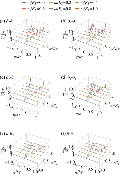
Figure 3: Dimensionless DSF tensor ${\widetilde{S}}_{ij}(q,\omega)=S_{ij}(q.\omega)E_{T}/k_{T}^{2}$, for $h_{x}/E_{T}=1.05$, $\mu/E_{T}=2.85$ $(n/n_{T}=1.00)$, $V_{0}/E_{T}=2$ $(a_{3D}\approx 159a_{0})$ and $k_{T}L=408.60$ corresponding to typical values for ${}^{40}{\rm K}$, with energy broadening $\delta/E_{T}=0.005$. Panels (a) through (d) show the charge-charge and spin-spin responses: (a) ${\hat{\rho}}$-${\hat{\rho}}$; (b) ${\hat{\sigma}}_{x}$-${\hat{\sigma}}_{x}$; (c) ${\hat{\sigma}}_{y}$-${\hat{\sigma}}_{y}$; and (d) ${\hat{\sigma}}_{z}$-${\hat{\sigma}}_{z}$. Panels (e) and (f) display the charge-spin ${\hat{\rho}}$-${\hat{\sigma}}_{+}$ and ${\hat{\rho}}$-${\hat{\sigma}}_{-}$ responses, respectively. The ${\hat{\sigma}}_{y}$-${\hat{\sigma}}_{y}$ response in (c) is weaker, hence it has a different scale. The gray dashed lines show the dispersing helical collective modes.

Response functions: Bragg scattering techniques have been used to measure velocities of charge and spin density collective modes [45, 46], as well as to identify spin-charge separation in ${}^{6}{\rm Li}$ [16, 17]. These experiments traditionally measure either charge or spin dynamical structure factors (DSF). Here, we go beyond that and investigate the spin-spin, charge-charge and spin-charge responses at $T=0$ via the DSF tensor ${S}_{ij}(q,\omega)=2\pi\sum_{m,p}\langle\Omega|{{\hat{\cal O}}_{i}(q)}|{m,p}\rangle\langle{m,p}|{{\hat{\cal O}}_{j}(-q)}|\Omega\rangle\delta(\omega-\varepsilon_{p,m}+\omega_{\Omega}),$ for the ground state $|\Omega\rangle$, in the Källén-Lehmann spectral representation [54, 55]. The operators ${\hat{\cal O}}_{i}(q)$, with $i=\{c,x,y,z\}$, are the charge $\hat{\cal O}_{c}(q)={\hat{\rho}}(q)$ and spin ${\cal O}_{\ell}(q)={\hat{\sigma}}_{\ell}(q)$ operators, where $\ell=\{x,y,z\}$ or $\ell=\{+,-,z\}$, with $+$ $(-)$ labelling the spin raising (lowering) operator ${\hat{\sigma}}_{+}$ $({\hat{\sigma}}_{-})$. The eigenstates of the bosonized Hamiltonian ${\hat{H}}$ given in Eq. (6) are $|m,p\rangle$ with corresponding eigenenergies $\varepsilon_{p,m}=|p|v_{m}$, while $\omega_{\Omega}$ is the ground state energy.

To calculate $S_{ij}(q,\omega)$, we implement the Moore-Penrose inverse [56, 57] and write the operators ${\hat{\cal O}}_{i}^{(r)}(q)$ in terms of the boson operators $d_{q,m}.$ When $q>0$, we obtain ${\hat{\cal O}}_{i}^{(r)}(q)=\sqrt{\frac{|q|L}{2\pi}}\sum_{m=1,2}\left(F_{im}^{(r)}(q)d_{-q,m}^{\dagger}+G_{im}^{(r)}(q)d_{q,m}\right),$ where the expression relating $q>0$ and $q<0$ is ${\hat{\cal O}}_{i}^{(r)}(-q)={\hat{\cal O}}_{i}^{\dagger(r)}(q)$. To obtain the matrix elements $\langle\Omega|{{\hat{\cal O}}_{i}(q)}|{m,p}\rangle$ and $\langle{m,p}|{{\hat{\cal O}}_{j}(-q)}|\Omega\rangle,$ we use ${\hat{\cal O}}_{j}(q)={\hat{\cal O}}_{j}^{(R)}(q)+{\hat{\cal O}}_{j}^{(L)}(q)$ leading to

$$S_{ij}(q,\omega)=\sum_{m}{\cal A}_{ij}^{(m)}(q)\delta(\omega-\varepsilon_{q,m}+\omega_{\Omega}),$$ (7)

where ${\cal A}_{ij}^{(m)}(q)$ plays the role of the spectral weight tensor with dimensions of squared-density (squared-length in 1D), $\varepsilon_{q,m}=|q|v_{m}$ is the collective mode energy, and we set $\omega_{\Omega}=0$ to be our energy reference. The Onsager reciprocal relation [58, 59] for the DSF tensor is $S_{ij}({q,\omega,k_{T},h_{x}})=\epsilon_{i}\epsilon_{j}S_{ji}({-q,\omega,-k_{T},-h_{x}}),$ where $\epsilon_{i}$ is the parity of operators ${\hat{\cal O}}_{i}(x,t)$ under time-reversal. For $i=c$ (charge density), $\epsilon_{i}=+1$, and for $i=\{x,y,z\}$ (spin density), $\epsilon_{i}=-1$.

In Fig. 3, we show matrix elements of ${\widetilde{S}}_{ij}(q,\omega)=S_{ij}(q,\omega)E_{T}/k_{T}^{2}=S_{ij}(q,\omega)/2m$ with energy broadening $\delta/E_{T}=0.05$. The parameters used are $h_{x}/E_{T}=1.50$, $\mu/E_{T}=2.85$ $(n/n_{T}=1.00)$, $V_{0}/E_{T}=2$ $(a_{3D}\approx 159a_{0})$, and $k_{T}L=408.60$ corresponding to typical values for ${}^{40}{\rm K}$. These values correspond to a point in the pink region of Fig. 2(a), where there are two collective modes.

In all panels of Fig. 3, the gray dashed lines represent the two dispersing helical modes. In panels (a) through (d), we show the charge-charge and spin-spin responses: (a) ${\hat{\rho}}$-${\hat{\rho}}$; (b) ${\hat{\sigma}}_{x}$-${\hat{\sigma}}_{x}$; (c) ${\hat{\sigma}}_{y}$-${\hat{\sigma}}_{y}$; and (d) ${\hat{\sigma}}_{z}$-${\hat{\sigma}}_{z}$. The ${\hat{\sigma}}_{y}$-${\hat{\sigma}}_{y}$ response in (c) is weaker, hence it has a different scale. In panels (e) and (f), we show the charge-spin ${\hat{\rho}}$-${\hat{\sigma}}_{+}$ and ${\hat{\rho}}$-${\hat{\sigma}}_{-}$ responses to reveal the helicity of the modes, since the responses are different. We verified that for $h_{x}\neq 0$ and $k_{T}=0$, the modes are non-helical, and that the only non-zero responses are ${\hat{\rho}}$-${\hat{\rho}}$, ${\hat{\sigma}}_{x}$-${\hat{\sigma}}_{x}$; ${\hat{\rho}}$-${\hat{\sigma}}_{x}$. Furthermore, for $h_{x}=0$ and any $k_{T}$, there is spin-charge separation, and the only non-zero responses are ${\hat{\rho}}$-${\hat{\rho}}$, and ${\hat{\sigma}}_{z}$-${\hat{\sigma}}_{z}$.

Conclusions: We studied the phase diagram and collective modes of interacting one-dimensional Fermi systems with spin-orbit coupling and Rabi fields. We indicated that topological quantum phase transitions of the Lifshitz type are induced by spin-orbit coupling and Rabi fields. We found that the phase diagram exhibits regions with two, one or zero helical collective modes, which correlate with the topology of the Fermi surface. We demonstrated that the velocities of the collective modes are nonanalytical as topological phase boundaries are crossed. We also identified the locus of spin-charge separation, and showed that, for non-zero spin-orbit coupling and Rabi fields, the collective modes are helical with mixed charge and spin density components. Lastly, we calculated the dynamical structure factors for the charge-charge, spin-charge and spin-spin responses, revealing the dispersions, spectral weights and helicities of collective modes, paving the way for their experimental detection in systems like ${}^{6}{\rm Li}$, ${}^{40}{\rm K}$ and ${}^{173}{\rm Yb}$.

References

- Tomonaga [1950] S.-I. Tomonaga, Remarks on Bloch’s Method of Sound Waves applied to Many-Fermion Problems, Progress of Theoretical Physics 5, 544 (1950).
- Luttinger [1963] J. M. Luttinger, An Exactly Soluble Model of a Many‐Fermion System, Journal of Mathematical Physics 4, 1154 (1963).
- Haldane [1981] F. D. M. Haldane, ’Luttinger liquid theory’ of one-dimensional quantum fluids. I. Properties of the Luttinger model and their extension to the general 1D interacting spinless Fermi gas, Journal of Physics C: Solid State Physics 14, 2585 (1981).
- Giamarchi [2003] T. Giamarchi, Quantum Physics in One Dimension (Oxford University Press, 2003).
- Altland and Simons [2023] A. Altland and B. Simons, Condensed Matter Field Theory, 3rd ed. (Cambridge University Press, 2023).
- Imambekov et al. [2012] A. Imambekov, T. L. Schmidt, and L. I. Glazman, One-dimensional quantum liquids: Beyond the Luttinger liquid paradigm, Rev. Mod. Phys. 84, 1253 (2012).
- Niemi and Walet [2005] A. J. Niemi and N. R. Walet, Splitting the gluon?, Phys. Rev. D 72, 054007 (2005).
- Faddeev and Niemi [2007] L. Faddeev and A. J. Niemi, Spin-charge separation, conformal covariance and the SU(2) Yang–Mills theory, Nuclear Physics B 776, 38 (2007).
- Chernodub and Niemi [2007] M. N. Chernodub and A. J. Niemi, Spin-charge separation and the Pauli electron, JETP Letters 85, 353 (2007).
- Diamandis et al. [1998] G. A. Diamandis, B. C. Georgalas, and N. E. Mavromatos, N=1 Supersymmetric Spin-charge Separation In Effective Gauge Theories Of Planar Magnetic Superconductors, Modern Physics Letters A 13, 387 (1998).
- Xiong [2015] C. Xiong, From the fourth color to spin-charge separation: Neutrinos and spinons, Modern Physics Letters A 30, 1530021 (2015).
- Kim et al. [1996] C. Kim, A. Y. Matsuura, Z.-X. Shen, N. Motoyama, H. Eisaki, S. Uchida, T. Tohyama, and S. Maekawa, Observation of Spin-Charge Separation in One-Dimensional SrCu, Phys. Rev. Lett. 77, 4054 (1996).
- Kim et al. [2006] B. J. Kim, H. Koh, E. Rotenberg, S. J. Oh, H. Eisaki, N. Motoyama, S. Uchida, T. Tohyama, S. Maekawa, Z. X. Shen, and C. Kim, Distinct spinon and holon dispersions in photoemission spectral functions from one-dimensional SrCuO2, Nature Physics 2, 397 (2006).
- Auslaender et al. [2002] O. M. Auslaender, A. Yacoby, R. de Picciotto, K. W. Baldwin, L. N. Pfeiffer, and K. W. West, Tunneling Spectroscopy of the Elementary Excitations in a One-Dimensional Wire, Science 295, 825 (2002).
- Auslaender et al. [2005] O. M. Auslaender, H. Steinberg, A. Yacoby, Y. Tserkovnyak, B. I. Halperin, K. W. Baldwin, L. N. Pfeiffer, and K. W. West, Spin-Charge Separation and Localization in One Dimension, Science 308, 88 (2005).
- Senaratne et al. [2022] R. Senaratne, D. Cavazos-Cavazos, S. Wang, F. He, Y.-T. Chang, A. Kafle, H. Pu, X.-W. Guan, and R. G. Hulet, Spin-charge separation in a one-dimensional Fermi gas with tunable interactions, Science 376, 1305 (2022).
- Cavazos-Cavazos et al. [2023] D. Cavazos-Cavazos, R. Senaratne, A. Kafle, and R. G. Hulet, Thermal disruption of a Luttinger liquid, Nature Communications 14, 3154 (2023).
- Sinova et al. [2015] J. Sinova, S. O. Valenzuela, J. Wunderlich, C. H. Back, and T. Jungwirth, Spin Hall effects, Rev. Mod. Phys. 87, 1213 (2015).
- Kawada et al. [2021] T. Kawada, M. Kawaguchi, T. Funato, H. Kohno, and M. Hayashi, Acoustic spin Hall effect in strong spin-orbit metals, Science Advances 7, eabd9697 (2021).
- Hasan and Kane [2010] M. Z. Hasan and C. L. Kane, Colloquium: Topological insulators, Rev. Mod. Phys. 82, 3045 (2010).
- Qi and Zhang [2011] X.-L. Qi and S.-C. Zhang, Topological insulators and superconductors, Rev. Mod. Phys. 83, 1057 (2011).
- Sato and Ando [2017] M. Sato and Y. Ando, Topological superconductors: a review, Reports on Progress in Physics 80, 076501 (2017).
- Scammell et al. [2022] H. D. Scammell, J. Ingham, M. Geier, and T. Li, Intrinsic first- and higher-order topological superconductivity in a doped topological insulator, Phys. Rev. B 105, 195149 (2022).
- Zeng et al. [2023] M. Zeng, D.-H. Xu, Z.-M. Wang, and L.-H. Hu, Spin-orbit coupled superconductivity with spin-singlet nonunitary pairing, Phys. Rev. B 107, 094507 (2023).
- Rashba and Sheka [1961] E. Rashba and V. Sheka, Combined resonance in electron InSb, Soviet Physics-Solid State 3, 1357 (1961).
- Dresselhaus [1955] G. Dresselhaus, Spin-Orbit Coupling Effects in Zinc Blende Structures, Phys. Rev. 100, 580 (1955).
- Bychkov and Rashba [1984] Y. A. Bychkov and É. I. Rashba, Properties of a 2D electron gas with lifted spectral degeneracy, JETP lett 39, 78 (1984).
- Sinova and MacDonald [2008] J. Sinova and A. MacDonald, Theory of Spin–Orbit Effects in Semiconductors, Semiconduct. Semimet. 82, 45 (2008).
- Schott et al. [2017] S. Schott, E. R. McNellis, C. B. Nielsen, H.-Y. Chen, S. Watanabe, H. Tanaka, I. McCulloch, K. Takimiya, J. Sinova, and H. Sirringhaus, Tuning the effective spin-orbit coupling in molecular semiconductors, Nature Communications 8, 15200 (2017).
- Chen et al. [2021] J. Chen, K. Wu, W. Hu, and J. Yang, Spin–Orbit Coupling in 2D Semiconductors: A Theoretical Perspective, The Journal of Physical Chemistry Letters 12, 12256 (2021).
- Marcellina et al. [2017] E. Marcellina, A. R. Hamilton, R. Winkler, and D. Culcer, Spin-orbit interactions in inversion-asymmetric two-dimensional hole systems: A variational analysis, Phys. Rev. B 95, 075305 (2017).
- Shcherbakov et al. [2021] D. Shcherbakov, P. Stepanov, S. Memaran, Y. Wang, Y. Xin, J. Yang, K. Wei, R. Baumbach, W. Zheng, K. Watanabe, T. Taniguchi, M. Bockrath, D. Smirnov, T. Siegrist, W. Windl, L. Balicas, and C. N. Lau, Layer- and gate-tunable spin-orbit coupling in a high-mobility few-layer semiconductor, Science Advances 7, eabe2892 (2021).
- Campbell et al. [2011] D. L. Campbell, G. Juzeliūnas, and I. B. Spielman, Realistic Rashba and Dresselhaus spin-orbit coupling for neutral atoms, Phys. Rev. A 84, 025602 (2011).
- Galitski and Spielman [2013] V. Galitski and I. B. Spielman, Spin–orbit coupling in quantum gases, Nature 494, 49 (2013).
- Lin et al. [2011] Y. J. Lin, K. Jiménez-García, and I. B. Spielman, Spin–orbit-coupled Bose–Einstein condensates, Nature 471, 83 (2011).
- Atala et al. [2014] M. Atala, M. Aidelsburger, M. Lohse, J. T. Barreiro, B. Paredes, and I. Bloch, Observation of chiral currents with ultracold atoms in bosonic ladders, Nature Physics 10, 588 (2014).
- Frölian et al. [2022] A. Frölian, C. S. Chisholm, E. Neri, C. R. Cabrera, R. Ramos, A. Celi, and L. Tarruell, Realizing a 1D topological gauge theory in an optically dressed BEC, Nature 608, 293 (2022).
- Cheuk et al. [2012] L. W. Cheuk, A. T. Sommer, Z. Hadzibabic, T. Yefsah, W. S. Bakr, and M. W. Zwierlein, Spin-Injection Spectroscopy of a Spin-Orbit Coupled Fermi Gas, Phys. Rev. Lett. 109, 095302 (2012).
- Mancini et al. [2015] M. Mancini, G. Pagano, G. Cappellini, L. Livi, M. Rider, J. Catani, C. Sias, P. Zoller, M. Inguscio, M. Dalmonte, and L. Fallani, Observation of chiral edge states with neutral fermions in synthetic Hall ribbons, Science 349, 1510 (2015).
- Kolkowitz et al. [2017] S. Kolkowitz, S. L. Bromley, T. Bothwell, M. L. Wall, G. E. Marti, A. P. Koller, X. Zhang, A. M. Rey, and J. Ye, Spin–orbit-coupled fermions in an optical lattice clock, Nature 542, 66 (2017).
- Campbell and Spielman [2016] D. L. Campbell and I. B. Spielman, Rashba realization: Raman with RF, New Journal of Physics 18, 033035 (2016).
- Huang et al. [2016] L. Huang, Z. Meng, P. Wang, P. Peng, S.-L. Zhang, L. Chen, D. Li, Q. Zhou, and J. Zhang, Experimental realization of two-dimensional synthetic spin–orbit coupling in ultracold Fermi gases, Nature Physics 12, 540 (2016).
- Valdés-Curiel et al. [2021] A. Valdés-Curiel, D. Trypogeorgos, Q. Y. Liang, R. P. Anderson, and I. B. Spielman, Topological features without a lattice in Rashba spin-orbit coupled atoms, Nature Communications 12, 593 (2021).
- Seo et al. [2012] K. Seo, L. Han, and C. A. R. Sá de Melo, Topological phase transitions in ultracold Fermi superfluids: The evolution from Bardeen-Cooper-Schrieffer to Bose-Einstein-condensate superfluids under artificial spin-orbit fields, Phys. Rev. A 85, 033601 (2012).
- Biss et al. [2022] H. Biss, L. Sobirey, N. Luick, M. Bohlen, J. J. Kinnunen, G. M. Bruun, T. Lompe, and H. Moritz, Excitation Spectrum and Superfluid Gap of an Ultracold Fermi Gas, Phys. Rev. Lett. 128, 100401 (2022).
- Sobirey et al. [2022] L. Sobirey, H. Biss, N. Luick, M. Bohlen, H. Moritz, and T. Lompe, Observing the influence of reduced dimensionality on fermionic superfluids, Phys. Rev. Lett. 129, 083601 (2022).
- Williamson [1936] J. Williamson, On the Algebraic Problem Concerning the Normal Forms of Linear Dynamical Systems, American Journal of Mathematics 58, 141 (1936).
- Lifshitz [1960] I. Lifshitz, Anomalies of electron characteristics of a metal in the high pressure region, Sov. Phys. JETP 11, 1130 (1960).
- Williams et al. [2013] R. A. Williams, M. C. Beeler, L. J. LeBlanc, K. Jiménez-García, and I. B. Spielman, Raman-Induced Interactions in a Single-Component Fermi Gas Near an -Wave Feshbach Resonance, Phys. Rev. Lett. 111, 095301 (2013).
- Livi et al. [2016] L. F. Livi, G. Cappellini, M. Diem, L. Franchi, C. Clivati, M. Frittelli, F. Levi, D. Calonico, J. Catani, M. Inguscio, and L. Fallani, Synthetic Dimensions and Spin-Orbit Coupling with an Optical Clock Transition, Phys. Rev. Lett. 117, 220401 (2016).
- Navon et al. [2021] N. Navon, R. P. Smith, and Z. Hadzibabic, Quantum gases in optical boxes, Nature Physics 17, 1334 (2021).
- Schymik et al. [2021] K.-N. Schymik, S. Pancaldi, F. Nogrette, D. Barredo, J. Paris, A. Browaeys, and T. Lahaye, Single Atoms with 6000-Second Trapping Lifetimes in Optical-Tweezer Arrays at Cryogenic Temperatures, Phys. Rev. Appl. 16, 034013 (2021).
- Schmidutz et al. [2014] T. F. Schmidutz, I. Gotlibovych, A. L. Gaunt, R. P. Smith, N. Navon, and Z. Hadzibabic, Quantum Joule-Thomson Effect in a Saturated Homogeneous Bose Gas, Phys. Rev. Lett. 112, 040403 (2014).
- Källén [1952] G. Källén, On the Definition of the Renormalization Constants in Quantum Electrodynamics, Helvetica Physica Acta 25, 417 (1952).
- Lehmann [1954] H. Lehmann, Über Eigenschaften von Ausbreitungsfunktionen und Renormierungskonstanten quantisierter Felder, Il Nuovo Cimento (1943-1954) 11, 342 (1954).
- Moore [1920] E. H. Moore, On the reciprocal of the general algebraic matrix, Bulletin of the American Mathematical Society 26, 394 (1920).
- Penrose [1955] R. Penrose, A generalized inverse for matrices, Mathematical Proceedings of the Cambridge Philosophical Society 51, 406–413 (1955).
- Onsager [1931a] L. Onsager, Reciprocal Relations in Irreversible Processes. I., Phys. Rev. 37, 405 (1931a).
- Onsager [1931b] L. Onsager, Reciprocal Relations in Irreversible Processes. II., Phys. Rev. 38, 2265 (1931b).