Collective Coordinate Models for 2-Vortex Shape Mode Dynamics

Abstract

Models are developed for the motion of charge-2 Abelian Higgs vortices through the 2-vortex moduli space ${\cal M}$, with the vortices excited by their shape mode oscillations. The models simplify to the well-known geodesic flow on ${\cal M}$, modified by a potential, when the mode oscillations are fast relative to the moduli space motion and their amplitudes are small. When the lowest-frequency mode is excited with a large amplitude, the geodesic flow is not a correct description. Instead, a chaotic, or even fractal, multi-bounce structure in vortex-vortex collisions is predicted.

1 Introduction

It has been known for some time that a unit-charge, critically coupled Abelian Higgs vortex (a BPS vortex) has a unique shape mode – a discrete, normalizable, radial oscillation mode whose frequency is below that of the continuum of radiation modes [2]. More recently, the shape modes of higher-charge, circularly symmetric (i.e. coincident) vortices have been determined. There are a finite number of these modes, the number increasing somewhat irregularly with the charge [3, 4, 5]. More recently still, the present authors studied how these shape modes and their frequencies vary over the 2-vortex moduli space [6]. We confirmed that the circularly symmetric 2-vortex has three shape modes, of which the upper two are degenerate. We also found that the degeneracy is broken as the vortices separate, and at a modest separation the highest mode disappears into the continuum spectrum. The remaining two modes, as the vortices separate further, are the in-phase and $180^{\circ}$ out-of-phase combinations of the radial shape modes of the two individual vortices. The in-phase combination has the lower frequency, but the frequencies merge at asymptotically large separation.

Over the 2-vortex moduli space, then, there is a non-degenerate lowest-frequency shape mode, and two higher-frequency modes, whose frequencies degenerate at vortex coincidence. Here, we first construct a model for the oscillatory dynamics of the lowest mode coupled to 2-vortex motion through the moduli space, and then a model for the dynamics of the two higher-frequency modes. We do not attempt to model a simultaneous excitation of all three modes.

We will need to use the curved metric on the 2-vortex moduli space. Samols investigated this metric for vortices moving in a plane, and discovered a formula for it just involving field data close to the vortex centres. This could be exploited to calculate the metric numerically [7]. The centre of mass decouples and has a flat metric, so the nontrivial factor is the moduli space ${\cal M}$ for the relative motion of the two vortices, with the centre of mass fixed. ${\cal M}$ is a smooth, two-dimensional manifold with $O(2)$ rotational symmetry – a surface of revolution – and its curvature is such that it can be embedded in $\mathbb{R}^{3}$ as a rounded cone whose apex corresponds to coincident vortices. The mode frequencies vary over ${\cal M}$, respecting this rotational symmetry.

The model for the lowest shape mode is simpler than the model for the upper modes. Its ingredients are the metric and the lowest mode’s frequency over ${\cal M}$. The resulting three-variable dynamics is not integrable, but provided the mode amplitude is small, and the motion through ${\cal M}$ is slow, we can perform an adiabatic analysis, because the mode oscillation is fast compared with the motion through ${\cal M}$. The reduced, two-variable dynamics is then integrable, using the conserved angular momentum and conserved energy. We find that the geodesic dynamics through moduli space that occurs in the absence of the mode excitation is modified by an induced potential energy function proportional to the mode’s frequency. Such a result is standard in the context of adiabatic dynamics.

The second model, for the excited upper pair of modes, is more sophisticated because of the conical structure of the frequencies around the point of vortex coincidence (the apex of ${\cal M}$), but it is only applicable when the two vortices are close together, as the highest mode (the third) disappears into the continuum spectrum when the vortices reach a modest separation. We can therefore approximate the moduli space as being flat, or of constant curvature, because its relevant inner region is a small neighbourhood of the apex. The generic dynamics is still quite complicated, and is best studied numerically.

This model simplifies if the relative vortex motion is restricted to be head-on, and it naturally joins up to a model for head-on motion in the outer region of moduli space, where the third mode is absent. We can therefore study a head-on collision where the vortices approach from infinity with the second mode excited. In the adiabatic approximation, this is similar to a head-on collision with the lowest mode excited, but the induced potential is repulsive rather than attractive.

Both the metric and mode frequencies over the moduli space ${\cal M}$ are only known numerically, but it is helpful to work with analytical formulae. We start in section 2, therefore, by deriving a good analytical approximation to the metric (and a simplified variant of this), and also present simple formulae for the frequencies of the three modes that fit the numerical results.

Section 3 discusses the model for the dynamics with the lowest mode excited, and presents numerical results for a head-on collision. The main change, in comparison with the geodesic flow describing the evolution of unexcited BPS vortices, is the appearance of an attractive mode-induced force. This has a great effect on vortex-vortex collisions. When the amplitude of oscillation is fairly large, the dynamics is complicated and exhibits a chaotic structure of multi-bounce windows reminiscent of what occurs in kink-antikink dynamics in one space dimension [8, 9, 10]. In this regime the geodesic dynamics fails completely. We also perform the small-amplitude adiabatic analysis and derive a reduced dynamics that is integrable. Here a head-on vortex collision always leads to scattering through $90^{\circ}$ (i.e. one bounce) and there are no multi-bounces.

Section 4 discusses the dynamics with the higher-frequency modes excited. Here, the adiabatic dynamics for small-amplitude oscillations is more interesting, because of the degeneracy of the second and third modes when the vortices coincide. Large-amplitude oscillations lead to complicated dynamics that we do not study in any detail. However we do present numerical results for head-on collisions where only the second mode is initially excited, and the excitation transfers to the third mode if the vortices pass through the circularly symmetric configuration at the apex of the moduli space, and scatter through $90^{\circ}$. In this case, the excitation of the mode gives rise to a force which changes sign at the apex. An initially repulsive interaction as the vortices approach changes into an attractive one as they separate at $90^{\circ}$. As a consequence, the vortices can stop and return – there is then 2-bounce (i.e. backwards) scattering. No further bounces are observed to occur.

In an appendix, we present some details of how our finite-dimensional models for the modes, coupled to the moduli space dynamics, emerge from the underlying field theory.

2 Approximate metric and mode frequencies on the 2-vortex moduli space

The lowest-order dynamics of two unit-charge BPS vortices is captured by geodesic motion on the moduli space ${\cal M}$ equipped with a curved metric originally found by Samols [7]. Here, the kinetic degrees of freedom of the vortices are excited but their internal shape modes are not.

In the physical 2-plane we use Cartesian coordinates $(X_{1},X_{2})$. The Higgs field $\phi$ of a centred 2-vortex has zeros at an unconstrained pair of locations $(X_{1},X_{2})=\pm(x_{1},x_{2})$, so we can denote a point in ${\cal M}$ (up to a sign) by Cartesian/polar coordinates $(x_{1},x_{2})=(\rho\cos\theta,\rho\sin\theta)$, and combine these into the complex coordinate $w=x_{1}+ix_{2}=\rho e^{i\theta}$. We refer to the real and imaginary axes in the $w$-plane (and also the $X_{1}$- and $X_{2}$-axis in the physical plane) as horizontal and vertical, respectively. $w$ is a natural complex coordinate on ${\cal M}$, with its magnitude and argument having the ranges $\rho\geq 0$ and $\theta\in[-\frac{1}{2}\pi,\frac{1}{2}\pi]$. The vortex centres (the Higgs field zeros) are precisely at $w$ and $-w$ in the physical 2-plane. Because vortices are indistinguishable, a shift of $\theta$ by $\pi$ maps a 2-vortex configuration into itself, which explains the limited range of $\theta$. A simple geodesic on ${\cal M}$ is where the vortices approach head-on along the horizontal axis, instantaneously coalesce at the origin, and then separate along the vertical axis. Here, $\theta$ jumps by $\frac{1}{2}\pi$.

The exact metric on ${\cal M}$ has the general, circularly symmetric form

$$ds^{2}=f^{2}(\rho)\left(d\rho^{2}+\rho^{2}d\theta^{2}\right).$$ (1)

For small and large $\rho$, the conformal factor is

$$f^{2}(\rho)=\left\{\begin{array}[]{cc}2\pi\gamma\rho^{2}&\rho\to 0\,,\\ 2\pi&\rho\to\infty\,.\end{array}\right.$$ (2)

Here, we have absorbed a factor of $2\pi$ into Samols’ original metric; $\gamma$ is approximately 0.433. For large $\rho$, the metric is asymptotically flat, with an exponentially small correction [11] that we neglect. Because of the range of $\theta$, the moduli space ${\cal M}$ is not asymptotically a plane, but an intrinsically flat cone, whose half-opening angle is $30^{\circ}$ (in the embedding in $\mathbb{R}^{3}$). ${\cal M}$ is globally a rounded cone – a flat cone whose apex is smoothly rounded off. The factor $\rho^{2}$ ensures that the metric is smooth at $\rho=0$. This is verified by changing to a coordinate $z$ proportional to $w^{2}$. $z$, whose argument has range $2\pi$, is a better global coordinate than $w$ on ${\cal M}$, as it ignores the sign of $w$, thereby taking into account the identity of the two vortices. If we write $z=x+iy=re^{i\varphi}$, then $x=r\cos\varphi$ and $y=r\sin\varphi$ are useful Cartesian coordinates on ${\cal M}$, even though ${\cal M}$ is curved. Then,

$$ds^{2}=\Omega(x,y)(dx^{2}+dy^{2})=\Omega(r)(dr^{2}+r^{2}d\varphi^{2})\,,$$ (3)

where the conformal factor $\Omega$ is a function only of $r=\sqrt{x^{2}+y^{2}}$.

A head-on collision, described earlier using the coordinate $w$, becomes simply a smooth motion along the $x$-axis from $+\infty$ to $-\infty$. However, because the geodesics on the asymptotically flat cone are simply straight lines in terms of $w$, we will often work with $w$ as the coordinate on ${\cal M}$, but at other times with $z$.

For our purposes, it is convenient to have good approximations to the metric on ${\cal M}$, enabling us to determine geodesics analytically, and hence vortex scattering in the absence of shape mode oscillations. To test these approximations, we compare the dependence of the scattering angle on impact parameter with the dependence obtained for the exact metric, presented graphically by Samols [7]. We consider two approximate metrics and will use these later when discussing small-amplitude oscillations of the vortex shape modes, and their effects on vortex dynamics and scattering. These approximations to the Samols geometry are novel and could be more broadly useful, e.g. for studying vortex quantum states, or approximating the moduli space metric for more than two vortices.

A striking result of Samols is that the rounded cone has an area deficit of $2\pi^{2}$ relative to the completed flat cone, extrapolated to its pointed apex [7]. We will reproduce this area deficit exactly with our approximate metrics.

2.1 Spherical cap approximation

For our first approximation, we attach a spherical cap to a truncated flat cone of opening angle $30^{\circ}$, maintaining a continuous tangent. The join needs to be at $\rho=\rho_{0}=\sqrt{6}$. The total metric is

$$ds^{2}_{(1)}=f^{2}_{(1)}(\rho)\left(d\rho^{2}+\rho^{2}d\theta^{2}\right)\,,$$ (4)

where

$$f^{2}_{(1)}(\rho)=\left\{\begin{array}[]{cc}\frac{6912\pi\rho^{2}}{(108+\rho^{4})^{2}}&\rho\leq\sqrt{6}\,,\\ &\\ 2\pi&\rho\geq\sqrt{6}\,.\end{array}\right.$$ (5)

$f^{2}_{(1)}(\rho)$ is continuous, and both functions in (5) have zero derivative at $\rho=\sqrt{6}$. To verify that for $\rho\leq\sqrt{6}$ it is a sphere metric, we introduce

$$z=\frac{1}{\sqrt{108}}w^{2}=\frac{1}{\sqrt{108}}\rho^{2}e^{i2\theta}\,.$$ (6)

In terms of $z$ we find that, for $\rho\leq\sqrt{6}$,

$$ds^{2}_{(1)}=\frac{6912\pi\rho^{2}}{(108+\rho^{4})^{2}}\left(d\rho^{2}+\rho^{2}d\theta^{2}\right)=\frac{16\pi\,dzd{\bar{z}}}{(1+z{\bar{z}})^{2}}\,.$$ (7)

The last expression represents the metric on a sphere with squared radius $4\pi$, with $z$ the stereographic coordinate.

Note that the spherical cap is restricted to $\rho\leq\sqrt{6}$ which implies that $|z|\leq\frac{1}{\sqrt{3}}$. Hence, on the cap, the maximal polar angle is $\mu=60^{\circ}$. (Use $|z|=\tan\frac{1}{2}\mu$ to verify this.) The boundary circles of the cap and the truncated cone have equal lengths $\sqrt{12\pi^{3}}$. Also $|z|$ has the correct range for the cap to join the flat cone with a continuous tangent.

Finally, the area deficit of the approximate metric (4) is correct. To see this we compare the area of the missing part of the flat cone,

$$A_{\rm{cone}}=\pi\int_{0}^{\sqrt{6}}2\pi\rho\,d\rho=6\pi^{2}\,,$$ (8)

where the prefactor is the range of $\theta$, with the area of the spherical cap

$$A_{\rm{cap}}=\pi\int_{0}^{\sqrt{6}}\frac{6912\pi\rho^{3}}{(108+\rho^{4})^{2}}\,d\rho=4\pi^{2}\,.$$ (9)

$A_{\rm{cap}}$ is one quarter of the area of a complete sphere of squared radius $4\pi$. The difference of the areas is

$$A_{\rm{cone}}-A_{\rm{cap}}=2\pi^{2}\,,$$ (10)

as required.

In this spherical cap approximation, a geodesic on ${\cal M}$ is formed from a straight line on the flat cone, joined to a segment of a great circle on the spherical cap, joined to another straight line on the cone. It will be convenient to consider the geodesics in the right-hand half $w$-plane that are reflection-symmetric with respect to the real axis. Any geodesic can be rotated to such a position. Some geodesics on the cone are sufficiently far from the vertex that they do not intersect the spherical cap. These geodesics are complete straight lines in the $w$-plane, parallel to the imaginary axis, describing 2-vortex motion without scattering.

For the approximate metric (4), with the conformal factor $f^{2}_{(1)}(\rho)$, a dynamical geodesic trajectory $w(t)=\rho(t)e^{i\theta(t)}$ arises as the solution of the equation of motion for a particle with Lagrangian

$$L=\frac{1}{2}f^{2}_{(1)}(\rho)(\dot{\rho}^{2}+\rho^{2}\dot{\theta}^{2})\,.$$ (11)

There are two constants of motion, the energy $E$ and angular momentum $J$. $E$ is the same expression as $L$, and $J=f^{2}_{(1)}(\rho)\rho^{2}\dot{\theta}$.

Asymptotically, $f^{2}_{(1)}(\rho)=2\pi$, as $\pi$ is the mass of a 1-vortex. The angular momentum of the incoming motion is $J=2\pi v_{\rm in}a$, where $v_{\rm in}$ is the speed of each vortex and $a$ the impact parameter (half the orthogonal separation of the incoming, parallel paths of the two vortices in the physical plane). The initial energy is $E=\pi v_{\rm in}^{2}$, so $J^{2}/E=4\pi a^{2}$. Any geodesic has a point of closest approach of the two vortices, where $\rho$ takes its minimum value $\tilde{\rho}$. Here $\dot{\rho}=0$, so $E=\frac{1}{2}f^{2}_{(1)}(\tilde{\rho})\tilde{\rho}^{2}\dot{\theta}^{2}$ and $J=f^{2}_{(1)}(\tilde{\rho})\tilde{\rho}^{2}\dot{\theta}$. $\dot{\theta}$ cancels in $J^{2}/E$, and conservation of $J^{2}/E$ implies that

$$f^{2}_{(1)}({\tilde{\rho}}){\tilde{\rho}}^{2}=2\pi a^{2}\,.$$ (12)

This relation between the closest approach and the impact parameter will be useful shortly. For a geodesic that does not intersect the spherical cap, $\tilde{\rho}$ is simply $a$.

Geodesics on the spherical cap are segments of great circles on the complete sphere. In terms of the stereographic coordinate $z$ on the cap, these great circles are a family of circles in the $z$-plane, having the algebraic equation

$$z\bar{z}+\beta(z+\bar{z})-1=0\,,$$ (13)

where the parameter $\beta$ is real and positive. This family is algebraically the linear join of the equatorial great circle $z\bar{z}-1=0$ and the line $z+\bar{z}=0$, which describes a great circle through the pole of the cap (the rounded cone’s apex). They are all great circles because they pass through the antipodal points $i$ and $-i$ on the sphere. As $|z|\leq\frac{1}{\sqrt{3}}$ on the spherical cap, the relevant range of $\beta$ is $\frac{1}{\sqrt{3}}\leq\beta\leq\infty$. For $\beta=\frac{1}{\sqrt{3}}$ the geodesic just touches the cap at $z=\frac{1}{\sqrt{3}}$, and for $\beta=\infty$ the geodesic passes through the pole, and represents a head-on collision of vortices.

For the conformal factor on the spherical cap (5), the relation giving the closest approach is

$$\frac{6912\pi{\tilde{\rho}}^{4}}{(108+{\tilde{\rho}}^{4})^{2}}=2\pi a^{2}\,,$$ (14)

so

$$\tilde{\rho}^{2}=\frac{12\sqrt{6}}{a}\left(1-\sqrt{1-\frac{a^{2}}{8}}\right)\,.$$ (15)

From this, we can determine the relation between $\beta$ and the impact parameter $a$. The closest approach of the circle (13) to the origin is where the circle crosses the real axis. This is where $z^{2}+2\beta z-1=0$, so $z=\sqrt{\beta^{2}+1}-\beta$. As $z=\frac{w^{2}}{\sqrt{108}}$, and $w=\tilde{\rho}$ at closest approach, we deduce that

$$\sqrt{\beta^{2}+1}-\beta=\frac{2\sqrt{2}}{a}\left(1-\sqrt{1-\frac{a^{2}}{8}}\right)\,,$$ (16)

which fortunately simplifies to

$$\beta=\sqrt{\frac{8}{a^{2}}-1}\,.$$ (17)

To understand vortex scattering, we focus on the coordinate $w$. The great circle segments in the $z$-plane become segments of quartic curves in the $w$-plane, with reflection symmetry in the real axis, although we do not need to know these curves in detail. Because the flat-cone parts of a geodesic are straight (in the coordinate $w$), scattering only occurs on the curved segment, i.e. on the spherical cap. The scattering angle depends on the change of direction of this segment, between its start and end points. The direction of an infinitesimal part of a segment is the argument of $dw$, and by reflection symmetry, the change of direction along this segment is directly related to the difference between the arguments of $dw$ and $d\bar{w}$, that is, to the argument of $\frac{dw}{d{\bar{w}}}$, evaluated at the endpoint of the segment.

To calculate the argument of $\frac{dw}{d{\bar{w}}}$, we note that $w=(108)^{1/4}\sqrt{z}$ so

$$dw=\frac{(108)^{1/4}dz}{2\sqrt{z}}\quad{\rm and}\quad d{\bar{w}}=\frac{(108)^{1/4}d{\bar{z}}}{2\sqrt{\bar{z}}}\,.$$ (18)

Therefore

$$\frac{dw}{d{\bar{w}}}=\sqrt{\frac{\bar{z}}{z}}\frac{dz}{d{\bar{z}}}\,.$$ (19)

Next, taking the differential of the equation (13) for a great circle segment, we find that

$$\frac{dz}{d{\bar{z}}}=-\frac{\beta+z}{\beta+\bar{z}}$$ (20)

so everywhere along the segment,

$$\frac{dw}{d{\bar{w}}}=-\sqrt{\frac{\bar{z}}{z}}\,\frac{\beta+z}{\beta+\bar{z}}\,.$$ (21)

The endpoints in the $z$-plane are where the circle (13) intersects the boundary circle of the spherical cap, $|z|=\frac{1}{\sqrt{3}}$. The endpoint with positive imaginary part is

$$z=\frac{1}{3\beta}(1+i\sqrt{3\beta^{2}-1})\,.$$ (22)

After some manipulation, we find from (21) the endpoint value

$$\arg\frac{dw}{d\bar{w}}=\pi+\arctan{\sqrt{3\beta^{2}-1}}-2\arctan\left(\frac{1}{2}\sqrt{3\beta^{2}-1}\right)\,,$$ (23)

and simple geometry shows that the scattering angle $\Theta$ along this geodesic is

$$\Theta=\pi-\arg\frac{dw}{d\bar{w}}=2\arctan\left(\frac{1}{2}\sqrt{3\beta^{2}-1}\right)-\arctan{\sqrt{3\beta^{2}-1}}\,.$$ (24)

Expressed in terms of the impact parameter $a$, using (17), this becomes

$$\Theta=2\arctan\sqrt{\frac{6}{a^{2}}-1}-\arctan\left(2\sqrt{\frac{6}{a^{2}}-1}\right)\,.$$ (25)

Finally, using the subtraction and double-angle formulae for the tangent function, we conclude that

$$\tan\Theta=\frac{(6-a^{2})^{3/2}}{a(9-a^{2})}\,.$$ (26)

This is valid for $a\leq\sqrt{6}$, and for larger impact parameters there is no scattering. As $a\to 0$, the scattering angle approaches $90^{\circ}$, the expected result for two vortices in a head-on collision [7]. Fig. 1 shows the scattering angle as a function of impact parameter, using this spherical cap approximation to the 2-vortex moduli space.

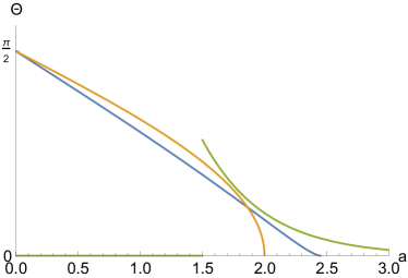
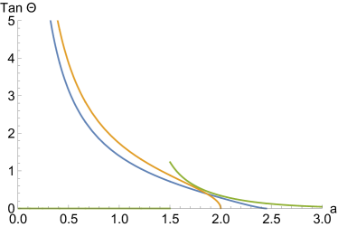
Figure 1: The scattering angle $\Theta$, and $\tan\Theta$, as functions of the impact parameter $a$: the spherical cap approximation (blue); the flat cap approximation (orange); the asymptotic approximation (green) [11].

2.2 Flat cap approximation

For our second, cruder approximation to the metric on ${\cal M}$, we attach a flat cap – a disc – to the top of a truncated flat cone, with the join at $\rho=\rho_{0}=2$. As before, $w=\rho e^{i\theta}$ with $\rho\geq 0$ and $\theta\in[-\frac{1}{2}\pi,\frac{1}{2}\pi]$. The total metric is

$$ds^{2}_{(2)}=f^{2}_{(2)}(\rho)\left(d\rho^{2}+\rho^{2}d\theta^{2}\right)$$ (27)

where

$$f^{2}_{(2)}(\rho)=\left\{\begin{array}[]{cc}\frac{1}{2}\pi\rho^{2}&\rho\leq 2\,,\\ &\\ 2\pi&\rho\geq 2\,.\end{array}\right.$$ (28)

This matches the asymptotic, flat-cone metric for $\rho\geq 2$. For $\rho\leq 2$, the change of coordinate $z=\frac{1}{4}w^{2}=\frac{1}{4}\rho^{2}e^{i2\theta}$ converts the metric to $ds^{2}=2\pi dzd\bar{z}$, with $|z|\leq 1$, a flat-disc metric. The missing part of the cone has area $4\pi^{2}$, whereas the disc has area $2\pi^{2}$. The area deficit is again $2\pi^{2}$, as required.

In this approximation, a geodesic has straight segments on the cone joined to a straight segment on the flat cap. Intrinsically, the tangent to the geodesic is continuous, even though the complete surface has a delta-function curvature at the join. In the $z$-plane, the geodesic segment on the flat cap is

$$z+\bar{z}=2X\,,$$ (29)

where the parameter $X$ is real and non-negative, and in the range $0\leq X\leq 1$. This segment, parallel to the imaginary axis, has the reflection symmetry that we imposed earlier.

In the $w$-plane, this geodesic segment becomes

$$w^{2}+{\bar{w}}^{2}=8X\,,$$ (30)

which is a rectangular hyperbola. Its closest approach to the origin is ${\tilde{\rho}}=2\sqrt{X}$. To find the relation between $X$ and the impact parameter $a$ we again use the conservation of $J^{2}/E$, leading to $f^{2}_{(2)}({\tilde{\rho}}){\tilde{\rho}}^{2}=2\pi a^{2}$, the analogue of (12), which implies that

$$\frac{1}{2}\pi{\tilde{\rho}}^{4}=2\pi a^{2}\,.$$ (31)

Therefore,

$$X=\frac{1}{2}a\,.$$ (32)

The scattering angle of the vortices depends only on the change of direction in the $w$-plane of the flat-cap geodesic segment between its endpoints, again given by $\frac{dw}{d\bar{w}}$. The differential of eq.(30) for this segment implies that

$$\frac{dw}{d\bar{w}}=-\frac{\bar{w}}{w}\,.$$ (33)

The endpoint (with positive imaginary part) in the $z$-plane is where $|z|=1$, so $z=X+i\sqrt{1-X^{2}}$, which converts to $w=\sqrt{2}\,({\sqrt{1+X}+i\sqrt{1-X}})$. Therefore

$$\arg\left(-\frac{\bar{w}}{w}\right)=\pi-2\arctan\left(\frac{\sqrt{1-X}}{\sqrt{1+X}}\right)\,,$$ (34)

so the scattering angle is

$$\Theta=2\arctan\left(\frac{\sqrt{1-X}}{\sqrt{1+X}}\right)\,,$$ (35)

and from the double-angle formula,

$$\tan\Theta=\frac{\sqrt{1-X^{2}}}{X}\,.$$ (36)

As $X=\frac{1}{2}a$, the scattering angle as a function of impact parameter $a$ in the flat cap approximation is

$$\Theta=\arctan\left(\frac{\sqrt{2-a}}{\sqrt{2+a}}\right)\,,\quad{\rm so}\quad\tan\Theta=\frac{\sqrt{4-a^{2}}}{a}\,,$$ (37)

both functions being shown in Fig. 1. This is not such a good approximation for the scattering angle as that obtained using the spherical cap approximation. In particular, the scattering angle (37) has an unwanted square root singularity as $a\to 2$.

2.3 Approximations for the mode frequencies

The squared frequency $\omega_{1}^{2}$ of the lowest mode varies with the vortex separation. It monotonically increases from approximately $\omega_{1}^{2}(0)=0.5378$ to $\omega_{1}^{2}(\infty)=0.7747$ (the squared frequency of the 1-vortex radial shape mode) as $\rho$ increases from $0$ to $\infty$. $\omega_{1}^{2}(\rho)$ can be approximated by the following rather simple function,

$$\omega_{1}^{2}(\rho)=\left\{\begin{array}[]{lc}\omega_{1}^{2}(0)+\frac{1}{R^{3}(R+2)}(\omega_{1}^{2}(\infty)-\omega_{1}^{2}(0))\rho^{4}&\rho\leq R\\ &\\ \omega_{1}^{2}(\infty)-\frac{2}{R+2}(\omega_{1}^{2}(\infty)-\omega_{1}^{2}(0))e^{2(R-\rho)}&\rho\geq R\,,\end{array}\right.$$ (38)

which is continuous and has continuous first derivative. It can be expressed in terms of the coordinate $r=\sqrt{x^{2}+y^{2}}$ using the relation $\rho^{2}=\sqrt{108}\,r$. The form of (38) is motivated by the facts that near the origin the squared frequency grows quadratically with $r$, i.e quartically with $\rho$, and that it approaches $\omega_{1}^{2}(\infty)$ exponentially with the vortex separation $2\rho$. Here, $R$ is a scale parameter, and a good fit is achieved with $R=2$. Because $\omega_{1}^{2}$ increases with the vortex separation, it will generate an attractive interaction.

The squared frequency of the second mode can be approximated as

$$\omega^{2}_{2}(\rho)=\omega^{2}_{2}(0)-(\omega^{2}_{2}(0)-\omega^{2}_{2}(\infty))\left(1-e^{-0.2\rho^{2}}\right),$$ (39)

where $\omega_{2}^{2}(0)=0.9747$ is the degenerate frequency of the second and third modes at coincidence, i.e. at the apex of the moduli space, and $\omega_{2}^{2}(\infty)=\omega_{1}^{2}(\infty)=0.7747$. $\omega_{2}$ depends linearly on $\rho^{2}$ near the apex, and continues smoothly to negative $\rho^{2}$ to give the frequency $\omega_{3}$ of the third mode. (In this context, $r$ is proportional to $|\rho^{2}|$.) Close to $\rho^{2}=-1$, the third mode hits the continuum threshold $\omega=1$, and disappears.

3 Model for the excited, lowest-frequency mode

3.1 Collective coordinate model

Here we consider a collective coordinate model for 2-vortex dynamics with the lowest mode excited. For vortices approaching from a large separation, this mode represents an in-phase superposition of the radial shape modes on each vortex.

This model is quite simple. Over the 2-vortex moduli space ${\cal M}$ with metric $ds^{2}=\Omega(x,y)(dx^{2}+dy^{2})$, we assume there is defined a harmonic oscillator with normal coordinate $\eta$ and position-dependent frequency $\omega_{1}(x,y)$. The following Lagrangian couples the excited oscillator to motion through ${\cal M}$:

$$L=\frac{1}{2}\Omega(x,y)({\dot{x}}^{2}+{\dot{y}}^{2})+\frac{1}{2}{\dot{\eta}}^{2}-\frac{1}{2}\omega_{1}^{2}(x,y)\eta^{2}\,.$$ (40)

There are no cross terms in the kinetic energy, because the moduli space directions are zero modes of the 2-vortex fields, whereas the oscillator direction is a positive-frequency shape mode, and these modes are orthogonal.

The equations of motion derived from $L$ are

$$\frac{d}{dt}(\Omega{\dot{x}})-\frac{1}{2}\partial_{x}\Omega({\dot{x}}^{2}+{\dot{y}}^{2})+\omega_{1}\partial_{x}\omega_{1}\,\eta^{2} = 0\,,$$ (41)

$$\frac{d}{dt}(\Omega{\dot{y}})-\frac{1}{2}\partial_{y}\Omega({\dot{x}}^{2}+{\dot{y}}^{2})+\omega_{1}\partial_{y}\omega_{1}\,\eta^{2} = 0\,,$$ (42)

$$\ddot{\eta}+\omega_{1}^{2}\eta = 0\,.$$ (43)

Equations (41)-(42) can be expanded out, giving

$$\Omega{\ddot{x}}+\frac{1}{2}\partial_{x}\Omega\,{\dot{x}}^{2}+\partial_{y}\Omega\,{\dot{x}}{\dot{y}}-\frac{1}{2}\partial_{x}\Omega\,{\dot{y}}^{2}+\omega_{1}\partial_{x}\omega_{1}\,\eta^{2} = 0\,,$$ (44)

$$\Omega{\ddot{y}}-\frac{1}{2}\partial_{y}\Omega\,{\dot{x}}^{2}+\partial_{x}\Omega\,{\dot{x}}{\dot{y}}+\frac{1}{2}\partial_{y}\Omega\,{\dot{y}}^{2}+\omega_{1}\partial_{y}\omega_{1}\,\eta^{2} = 0\,.$$ (45)

Here, the coefficients of the quadratic terms in velocity (divided by $\Omega$) encode the Levi-Civita connection on ${\cal M}$.

3.2 Numerical results

For the numerical analysis of this model we use the spherical cap approximation to $\Omega$, i.e. to the geometry of ${\cal M}$, and the approximation (38) for $\omega_{1}^{2}$. Both have rotational symmetry. For simplicity, we restrict ourselves to head-on collisions. Thus, it is consistent to put $y\equiv 0$ identically in (44) and identify positive $x$ with motion of the vortex pair along the horizontal axis while negative $x$ corresponds to motion along the vertical axis. Each passage through $x=0$ corresponds to $90^{\circ}$ scattering, and we call this a bounce. For this restricted motion,

$$\Omega{\ddot{x}}+\frac{1}{2}\partial_{x}\Omega\,{\dot{x}}^{2}+\omega_{1}\partial_{x}\omega_{1}\,\eta^{2} = 0\,,$$ (46)

$$\ddot{\eta}+\omega_{1}^{2}\eta = 0\,.$$ (47)

We assume that at $t=0$ the vortices are well separated along the horizontal axis and approaching each other. In our numerics we assumed $x(0)=3$, corresponding to an initial vortex separation $2\rho\approx 11$, and $v_{\rm in}=-{\dot{x}}(0)>0$. Because the mode-mediated force between the vortices is always attractive there is at least one collision, i.e. $x(t)=0$ at least once.

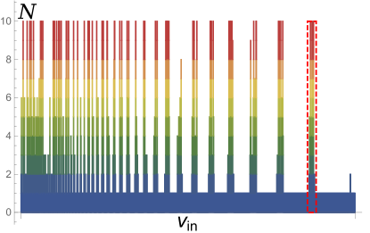
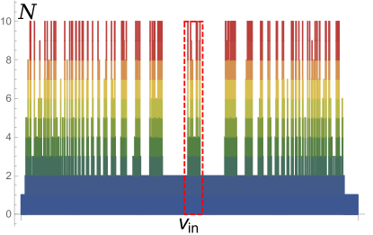
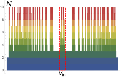
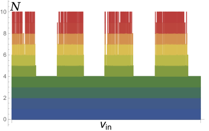
Figure 2: Number of bounces $N$ as a function of initial velocity $v_{\rm in}$. Here $N=10$ denotes 10 or more bounces. Upper left: multi-bounces immersed in 1-bounce windows, $v_{\rm in}\in[0,0.1]$; Upper right: multi-bounces immersed in 2-bounce windows, $v_{\rm in}\in[0.0862,0.088]$; Bottom left: multi-bounces immersed in 3-bounce windows, $v_{\rm in}\in[0.0870892,0.0871576]$; Bottom right: multi-bounces immersed in 4-bounce windows, $v_{\rm in}\in[0.087122032,0.0871248364]$.

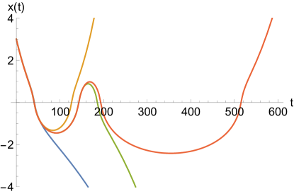
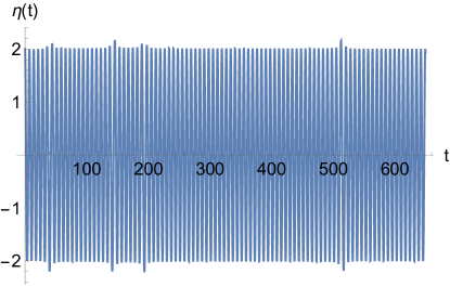
Figure 3: Left: examples of trajectories $x(t)$ of the 2-vortex modulus: 1-bounce, $v_{\rm in}=0.086$; 2-bounce, $v_{\rm in}=0.087$; 3-bounce, $v_{\rm in}=0.08757$ and 4-bounce, $v_{\rm in}=0.087571687055$. Right: evolution of the mode amplitude $\eta(t)$ for the 4-bounce solution.

The lowest mode is excited with initial amplitude $\eta(0)=2$ and $\dot{\eta}(0)=0$. $v_{\rm in}$ is then varied. One should remember that $v_{\rm in}$ is not the initial velocity of vortices in the physical plane, although the difference is rather small. The relation between the variables $\rho$ and $x$ gives

$$v_{\rm in}^{\rm phys}=\left(\frac{27}{4}\right)^{1/4}\frac{v_{\rm in}}{\sqrt{x(0)}}=\left(\frac{3}{4}\right)^{1/4}v_{\rm in}\,.$$ (48)

Our main result is that we find a chaotic structure in the scattering as $v_{\rm in}$ increases. The usual $90^{\circ}$ scattering (1-bounce) arising from the geodesic approximation is, in a rather chaotic way, replaced by multi-bounce windows, where colliding vortices form a quasi-bound state performing $N$ bounces – each being a $90^{\circ}$ scattering. For sufficiently large amplitude, the interchanging sequence of 1-bounce and multi-bounce windows starts from arbitrary small initial velocity and ends when $v_{\rm in}$ exceeds a critical velocity $v_{\rm cr}$. For $\eta(0)=2$ we find that $v_{\rm cr}=0.0988$, and for $v_{\rm in}>v_{\rm cr}$ we observe only single bounces, see Fig. 2, upper left. The figure shows the number of bounces (from 1 to $N\geq 10$) for initial velocities in the range $v_{\rm in}\in[0,0.1]$.

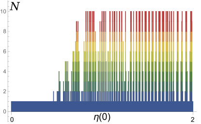
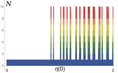
Figure 4: Number of bounces as a function of initial amplitude of the mode in the range $\eta(0)\in[0,2]$. Left: $v_{\rm in}=0.005$; Right: $v_{\rm in}=0.015$.

This chaotic structure has an approximately self-similar pattern. In Fig. 2, upper right, we show the $N\geq 3$ bounces immersed among 2-bounce scatterings, for $v_{\rm in}\in[0.0862,0.088]$. This structure repeats. The lower panels of Fig. 2 show $N\geq 4$ bounces immersed among 3-bounce scatterings, for $v_{\rm in}\in[0.0870892,0.0871576]$ and $N\geq 5$ bounces immersed among 4-bounce scatterings, for $v_{\rm in}\in[0.087122032,0.0871248364]$.

In Fig. 3, left, we show examples of 1-, 2-, 3- and 4-bounce solutions $x(t)$ for $v_{\rm in}=0.086,0.087,0.08757$ and $0.087571687055$ respectively. Clearly, a tiny change in the initial conditions can lead to a dramatic change in the scattering. In Fig. 3, right, we plot the time evolution $\eta(t)$ of the mode amplitude for this 4-bounce solution. The maximum amplitude is almost constant but briefly grows during the collisions.

In Fig. 4 we show how the structure of bounces changes if we vary the initial mode amplitude $\eta(0)$ but fix the initial velocity $v_{\rm in}$. For example, for $v_{\rm in}=0.05$ the first multi-bounce occurs when $\eta(0)=0.504$ whereas for $v_{\rm in}=0.15$ it occurs when $\eta(0)=0.826$. For sufficiently small values of the amplitude there is always a regime with one bounce, i.e. a single $90^{\circ}$ scattering. In this quasi-geodesic regime the geodesic dynamics is only softly modified by the mode excitation, making the vortex-vortex collision faster; see Fig. 5, where we plot the time $T$ at which the trajectory reaches $x=-3$, starting from $x=3$. $T$ decreases as the initial amplitude of the mode grows, a consequence of the attractive force triggered by the non-zero mode amplitude. However, above a critical value of $\eta(0)$ the chaotic multi-bounce behaviour starts. At this point, $T$ jumps and the geodesic approximation breaks down completely. Not surprisingly, the quasi-geodesic regime is larger if $v_{\rm in}$ is larger. In the next subsection we will analyze this regime from an adiabatic point of view.

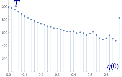
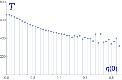
Figure 5: Collision time $T$ as a function of the initial amplitude of the mode $\eta(0)$. $T$ is the time for the trajectory to reach $x=-3$, starting from $x=3$. Left: $v_{\rm in}=0.010$; Right: $v_{\rm in}=0.015$.

We remark that although the positions of the 1-bounce and multi-bounce collisions are quite sensitive to details of our collective model, that is, to changes of $\omega_{1}$ and $\Omega$, the chaotic multi-bounce structure is robust. Therefore we expect that vortex scattering in the full field theory with the lowest mode excited will exhibit the same features. In fact, preliminary results from numerical simulations of the field theory confirm the validity of our collective model [12].

All these results resemble what is observed in kink-antikink scattering in $\phi^{4}$ theory in (1+1) dimensions. There also, there is a chaotic sequence of multi-bounce windows and annihilation regions called bion chimneys [8, 9], with a strong dependence on the initial relative velocity of the kinks, and on the initial shape mode amplitude. In particular, the accumulation of 2-vortex multi-bounces as $v_{\rm in}$ tends to 0 (for fixed initial mode amplitude) possesses its counterpart in scatterings between a wobbling kink and antikink [13]. Such a chaotic pattern is explained in terms of a resonant energy transfer mechanism between the kink kinetic energy and shape mode energy [8, 9], and it has recently been established that a collective model with two degrees of freedom explains the observed dynamics well [10]. The main difference from vortices is that the chaotic behaviour in kink-antikink collisions occurs even without an initial excitation of the shape mode, because there is automatically an attractive force between kink and antikink. For the BPS 2-vortices, an excitation of the lowest shape mode is needed to generate an attraction.

3.3 Adiabatic approximation

We now treat the oscillator as a fast variable, and the motion through ${\cal M}$ as slow. It is also important that the mode amplitude is relatively small. More precisely, we assume that $\omega_{1}$ and $\Omega$, together with their $x$- and $y$-derivatives, are $O(1)$, and that ${\dot{x}}$ and ${\dot{y}}$ are $O(\varepsilon)$, with $\varepsilon$ small. We wish ${\ddot{x}}$ and ${\ddot{y}}$ to be $O(\varepsilon^{2})$, and see from eqs.(44) and (45) that the oscillator amplitude $\eta$ needs to be $O(\varepsilon)$. With these assumptions, the solution of eq.(43) for the oscillator, in the adiabatic approximation, takes the form

$$\eta(t)=A(x(t),y(t))\,\cos\left(\int_{0}^{t}\omega_{1}(x(t^{\prime}),y(t^{\prime}))\,dt^{\prime}\right)\,,$$ (49)

where we have chosen the time origin to coincide with an instantaneous maximal amplitude of $\eta$. The integral is along a path through ${\cal M}$ that is still to be determined using the equations for $x$ and $y$. The amplitude $A$ is also yet to be determined, but only depends on the position in ${\cal M}$ at time $t$, and not on the path through ${\cal M}$. Clearly, $A$ needs to be $O(\varepsilon)$.

Differentiating (49) twice with respect to time, we find that

$$\ddot{\eta}+\omega_{1}^{2}\eta={\ddot{A}}\cos\left(\int_{0}^{t}\omega_{1}(x(t^{\prime}),y(t^{\prime}))\,dt^{\prime}\right)-\left(2\omega_{1}{\dot{A}}+A{\dot{\omega}_{1}}\right)\sin\left(\int_{0}^{t}\omega_{1}(x(t^{\prime}),y(t^{\prime}))\,dt^{\prime}\right)\,,$$ (50)

where $\dot{\omega}_{1}$ is the total time-derivative of $\omega_{1}$ along the path. The first term on the right-hand side is $O(\varepsilon^{3})$, and can be neglected relative to the remaining terms, which are $O(\varepsilon^{2})$. Equation (43) for the oscillator is therefore satisfied provided that

$$2\omega_{1}{\dot{A}}+A{\dot{\omega}_{1}}=0\,.$$ (51)

The solution is

$$A=\frac{C}{\sqrt{\omega_{1}}}$$ (52)

with $C$ a constant, so $A$ is indeed like $\omega_{1}$, being just a function of the instantaneous position $(x(t),y(t))$. $C$ is the adiabatic invariant of the oscillator, remaining constant despite the oscillator having a varying frequency $\omega_{1}$ along the path in ${\cal M}$. For consistency, $C$ is $O(\varepsilon)$.

We now derive the reduced, adiabatic equations of motion for $x$ and $y$, using the approximate solution for the oscillator

$$\eta(t)=\frac{C}{\sqrt{\omega_{1}(x(t),y(t))}}\,\cos\left(\int_{0}^{t}\omega_{1}(x(t^{\prime}),y(t^{\prime}))\,dt^{\prime}\right)\,.$$ (53)

We need to take the time-average of $\eta^{2}$ over one period of the oscillator, to derive the average force that acts. This is $\langle\eta^{2}\rangle=\frac{1}{2}A^{2}=\frac{1}{2}\frac{C^{2}}{\omega_{1}}$. The reduced equations are therefore eqs.(44) and (45) with $\omega_{1}\eta^{2}$ replaced by $\frac{1}{2}C^{2}$. More convenient is to give the reduced Lagrangian, from which these equations follow, namely

$$L_{\rm red}=\frac{1}{2}\Omega(x,y)({\dot{x}}^{2}+{\dot{y}}^{2})-\frac{1}{2}C^{2}\omega_{1}(x,y)\,.$$ (54)

The constant $C^{2}$ is determined by the oscillator’s initial conditions, and implicitly, ${\dot{x}}^{2},{\dot{y}}^{2}$ and $C^{2}$ are all $O(\varepsilon^{2})$.

In summary, the oscillator dynamics generates a potential energy $\frac{1}{2}C^{2}\omega_{1}(x,y)$ that, together with the conformal factor $\Omega$, governs adiabatic motion through ${\cal M}$. This motion has the conserved energy

$$E_{\rm red}=\frac{1}{2}\Omega(x,y)({\dot{x}}^{2}+{\dot{y}}^{2})+\frac{1}{2}C^{2}\omega_{1}(x,y)\,,$$ (55)

which matches the conserved energy for the original Lagrangian (40) if we use the time-averaged oscillator energy. The latter is

$$\langle E_{\rm osc}\rangle=\frac{1}{2}A^{2}\omega_{1}^{2}=\frac{1}{2}C^{2}\omega_{1}\,,$$ (56)

where we have ignored the contribution of $\dot{A}$ relative to that of $A$. Note that the adiabatic invariant $C^{2}$ is $\frac{2}{\omega_{1}}\langle E_{\rm osc}\rangle$.

The discussion so far has needed to assume no symmetry property for $\omega_{1}$ and $\Omega$. However, in the context of the 2-vortex moduli space ${\cal M}$ – the rounded cone – both the frequency $\omega_{1}$ of the lowest shape mode and the metric conformal factor $\Omega$ have $O(2)$ rotational symmetry. It is therefore convenient to use the polar coordinates $x=r\cos\varphi,\,y=r\sin\varphi$ on ${\cal M}$, and the radial functions $\omega_{1}(r)$ and $\Omega(r)$. $r=0$ is the apex of ${\cal M}$, where the vortices are coincident, and $r$ extends to $+\infty$ as the vortices separate. $\omega(r)$ and $\Omega(r)$ are positive and have zero derivative at $r=0$. The angle $\varphi$ has the range $\varphi\in[-\pi,\pi]$.

The Lagrangian (40) for the shape mode dynamics coupled to the moduli space motion simplifies as a result of the rotational symmetry, and in particular, the reduced Lagrangian (54) simplifies to

$$L_{\rm red}=\frac{1}{2}\Omega(r)({\dot{r}}^{2}+r^{2}{\dot{\varphi}}^{2})-\frac{1}{2}C^{2}\omega_{1}(r)\,.$$ (57)

There are two constants of motion for $L_{\rm red}$, the energy and angular momentum

$$E = \frac{1}{2}\Omega(r)({\dot{r}}^{2}+r^{2}{\dot{\varphi}}^{2})+\frac{1}{2}C^{2}\omega_{1}(r)\,,$$ (58)

$$J = \Omega(r)r^{2}{\dot{\varphi}}\,.$$ (59)

After eliminating ${\dot{\varphi}}$ from the energy in favour of the angular momentum, the radial motion can be found by quadrature, provided we know both $\omega_{1}(r)$ and $\Omega(r)$, and all the initial data, including that for the oscillator.

As $\omega_{1}(r)$ is an increasing function of $r$, the potential is attractive, but the effective potential in the reduced dynamics,

$$V_{\rm red}=\frac{1}{2}C^{2}\omega_{1}(r)+\frac{J^{2}}{2\Omega(r)r^{2}}\,,$$ (60)

includes a centrifugal term, so can be can be attractive or repulsive. There can therefore be both bounded and scattering solutions for the adiabatic 2-vortex dynamics when the lowest shape mode is excited. This contrasts with the dynamics in the absence of shape mode oscillations, where the motion on ${\cal M}$ follows geodesics, and consists purely of scattering trajectories [7]. The existence of bound orbits depends on the ratio between the adiabatic invariant and the angular momentum, $C/J$.

The simplest motion, using this adiabatic approximation, is a head-on collision, with the vortices approaching from a large separation at some finite velocity. The timing for this is shown in Fig. 5.

4 Model for higher-frequency shape modes

4.1 Collective coordinate model

Recall that the higher-frequency shape modes (the second and third modes) become degenerate at the apex of the moduli space ${\cal M}$, and that the third mode enters the continuum close to the apex. A model for the higher-frequency modes needs to allow for their interaction, as their frequencies are close together, but it needs to be constructed only in the inner region of ${\cal M}$, around the apex. Here we can approximate the geometry of ${\cal M}$ by a flat cap (the spherical cap approximation would be a refinement), and the mode frequencies can be approximated as having a linear dependence on $|z|$, where $z=x+iy=re^{i\varphi}$ is the suitably normalized complex coordinate centred at the apex of ${\cal M}$.

The coordinate $z$ is a parametrization for the 2-vortex gauge and Higgs fields over ${\cal M}$; similarly the vector space of higher-frequency shape modes and their amplitudes, involving deformations of the gauge and Higgs fields and a background gauge condition, can be parametrized by an abstract pair of amplitudes $\zeta$ and $\chi$. These are initially complex, but we will impose a reality condition below. There is $O(2)$ rotational symmetry about $z=0$, and the modes transform at $z=0$ as a doublet of $O(2)$.

The potential energy for the modes is constructed using the $2\times 2$ hermitian matrix

$$M=\begin{pmatrix}\lambda&\alpha(x-iy)\\ \alpha(x+iy)&\lambda\end{pmatrix}=\begin{pmatrix}\lambda&\alpha z^{*}\\ \alpha z&\lambda\end{pmatrix}\,,$$ (61)

where $\lambda$ and $\alpha$ are real and positive constants; $\lambda$ is the degenerate eigenvalue of $M$ when $z=0$. The eigenvalues of $M$ split for $z\neq 0$, becoming $\lambda\pm\alpha|z|$. The complete Lagrangian of the model, with standard kinetic terms and a quadratic potential obtained using $M$, is

$$L = \frac{1}{2}\left\{{\dot{z}}^{*}{\dot{z}}+{\dot{\zeta}}^{*}{\dot{\zeta}}+{\dot{\chi}}^{*}{\dot{\chi}}-(\zeta^{*}\ \chi^{*})\begin{pmatrix}\lambda&\alpha z^{*}\\ \alpha z&\lambda\end{pmatrix}\begin{pmatrix}\zeta\\ \chi\end{pmatrix}\right\}$$ (62)

$$= \frac{1}{2}\left\{{\dot{r}}^{2}+r^{2}{\dot{\varphi}}^{2}+{\dot{\zeta}}^{*}{\dot{\zeta}}+{\dot{\chi}}^{*}{\dot{\chi}}-(\zeta^{*}\ \chi^{*})\begin{pmatrix}\lambda&\alpha re^{-i\varphi}\\ \alpha re^{i\varphi}&\lambda\end{pmatrix}\begin{pmatrix}\zeta\\ \chi\end{pmatrix}\right\}\,.$$

$\zeta$ and $\chi$ are the (undiagonalised) amplitudes of the modes whose frequencies are controlled by the $z$-dependent matrix $M$. Before looking at the equations of motion it helps to say more about the eigenvectors of $M$.

A generic $2\times 2$ hermitian matrix is of the form $M=\lambda+{\bf a}\cdot{\boldsymbol{\sigma}}=\lambda+a_{1}\sigma_{1}+a_{2}\sigma_{2}+a_{3}\sigma_{3}$, where $\sigma_{1}\,,\sigma_{2}\,,\sigma_{3}$ are the Pauli matrices. This has eigenvalues $\lambda\pm|{\bf a}|$, so the eigenvalues are degenerate only when ${\bf a}=0$. Generally, in a family of $2\times 2$ hermitian matrices, the eigenvalues degenerate on a submanifold of real codimension 3 in the parameter space. But for our problem we have only two real moduli, and degeneracy still occurs. The reason is that $M$ is a family of hermitian matrices with a “real” structure. If $a_{2}$ were zero, then $M$ would be manifestly real, and we could seek real eigenvectors. Degeneracy would then occur when $a_{1}=a_{3}=0$, a codimension-2 condition. It is more convenient in our model to set $a_{3}=0$, as this simplifies the eigenvectors, but there is still a “real” structure, and eigenvalue degeneracy occurs at $z=0$, a single point in the 2-dimensional moduli space. The real structure occurs, because for the vortices in the abelian Higgs model, the shape mode eigenfunctions are derived from eigenfunctions of a scalar Schrödinger operator with a real potential [6].

More concretely, the model Lagrangian (62) is invariant under $\zeta^{*}\leftrightarrow\chi$ and we can impose the “reality” condition $\zeta^{*}=\chi$. This gives a consistent truncation of the equations of motion. Moreover, it is consistent to impose this condition on the Lagrangian. We therefore restart from the Lagrangian (62), with $\zeta^{*}$ replaced by $\chi$ (and $\zeta$ replaced by $\chi^{*}$),

$$L=\frac{1}{2}{\dot{z}}^{*}{\dot{z}}+{\dot{\chi}}^{*}{\dot{\chi}}-\lambda\chi^{*}\chi-\frac{1}{2}\alpha z^{*}\chi^{2}-\frac{1}{2}\alpha z\chi^{*\,2}\,.$$ (63)

The equations of motion now simplify to

$${\ddot{z}}+\alpha\chi^{2} = 0\,,$$ (64)

$${\ddot{\chi}}+\lambda\chi+\alpha z\chi^{*} = 0\,,$$ (65)

and there is a conserved energy

$$E=\frac{1}{2}{\dot{z}}^{*}{\dot{z}}+{\dot{\chi}}^{*}{\dot{\chi}}+\lambda\chi^{*}\chi+\frac{1}{2}\alpha z^{*}\chi^{2}+\frac{1}{2}\alpha z\chi^{*\,2}\,.$$ (66)

Equation (64) implies that the mode oscillations affect the moduli space motion, and eq.(65) implies that the mode oscillation frequencies at each instant depend on the location $z$ in moduli space. These coupled equations can probably not be solved analytically, but only numerically.

4.2 Adiabatic approximation

However, we can treat the dynamics adiabatically, assuming that $z$ varies on a timescale much longer than the inverse of the oscillation frequencies $\sqrt{\lambda\pm\alpha|z|}$. This is just a little more sophisticated than the adiabatic treatment of the lowest-frequency oscillation mode, in section 3. The scaling that makes an adiabatic analysis possible is to suppose that $z$, $\lambda$ and $\alpha$ are $O(1)$, with $\lambda\pm\alpha|z|$ remaining bounded away from zero, and that ${\dot{z}}=O(\varepsilon)$ and ${\ddot{z}}=O(\varepsilon^{2})$, with $\varepsilon$ small. This requires the mode amplitudes $|\zeta|$ and $|\chi|$ to be $O(\varepsilon)$, i.e. small, but their oscillation frequencies are $O(1)$.

To proceed, we need a basis of eigenvectors of the matrix $M$ appearing in eq.(62). The eigenvectors/eigenvalues are given by

$$\begin{pmatrix}\lambda&\alpha re^{-i\varphi}\\ \alpha re^{i\varphi}&\lambda\end{pmatrix}\begin{pmatrix}\zeta\\ \chi\end{pmatrix}=\nu\begin{pmatrix}\zeta\\ \chi\end{pmatrix}\,,$$ (67)

so the eigenvalues are $\nu_{+}=\lambda+\alpha r$ and $\nu_{-}=\lambda-\alpha r$, with respective eigenvectors

$$\begin{pmatrix}\zeta\\ \chi\end{pmatrix}=\begin{pmatrix}1\\ e^{i\varphi}\end{pmatrix}\quad{\rm and}\quad\begin{pmatrix}\zeta\\ \chi\end{pmatrix}=\begin{pmatrix}1\\ -e^{i\varphi}\end{pmatrix}$$ (68)

of squared norm 2. However, these eigenvectors don’t satisfy the reality condition $\zeta^{*}=\chi$ until we multiply by a suitable phase factor (which doesn’t affect their orthonormality). The “real” eigenvectors are

$$V_{+}(\varphi)=\pm\begin{pmatrix}e^{-\frac{1}{2}i\varphi}\\ e^{\frac{1}{2}i\varphi}\end{pmatrix}\quad{\rm and}\quad V_{-}(\varphi)=\pm\begin{pmatrix}ie^{-\frac{1}{2}i\varphi}\\ -ie^{\frac{1}{2}i\varphi}\end{pmatrix}\,,$$ (69)

where the phases are fixed, but there remains an ambiguity in sign. Note that when $\varphi$ increases by $2\pi$, the sign of each of these eigenvectors reverses. For a given $r\neq 0$, the eigenspaces are therefore Möbius bundles over the circle parametrised by $\varphi$. In fact, these bundles extend to the entire punctured plane $r\neq 0$.

It is significant that these Möbius bundles join up smoothly at the origin, where the eigenvalues degenerate. There is continuity of the eigenvectors and eigenvalues along any line in the $z$-plane that passes through the origin. Consider, for example, the line $y=0$ with $x$ running from a positive to a negative value. There is a constant eigenvector $(1,1)^{\rm T}$ along this line with eigenvalue $\lambda+\alpha x$, and another constant eigenvector $(i,-i)^{\rm T}$ with eigenvalue $\lambda-\alpha x$. To check this, one has to identify a point with negative $x$ as having $r=|x|$ and $\varphi=\pi$. Along this line the lower eigenvalue runs smoothly into the upper eigenvalue, and vice versa. Such eigenvalue crossing naturally occurs, because the eigenvalue spectrum exhibits a conical structure over a neighbourhood of the origin.

We next express the dynamical mode amplitudes in terms of the eigenvectors as

$$\begin{pmatrix}\zeta\\ \chi\end{pmatrix}=a_{+}(t)V_{+}(\varphi(t))+a_{-}(t)V_{-}(\varphi(t))\,,$$ (70)

where $a_{+}$ and $a_{-}$ are real. (An arbitrary initial sign choice for the eigenvectors is made.) The time-derivative is

$$\frac{d}{dt}\begin{pmatrix}\zeta\\ \chi\end{pmatrix}={\dot{a}}_{+}V_{+}+a_{+}\partial_{\varphi}V_{+}\,{\dot{\varphi}}+{\dot{a}}_{-}V_{-}+a_{-}\partial_{\varphi}V_{-}\,{\dot{\varphi}}\,.$$ (71)

The eigenvectors have the simple $\varphi$-derivatives

$$\partial_{\varphi}V_{+}=-\frac{1}{2}V_{-}\quad{\rm and}\quad\partial_{\varphi}V_{-}=\frac{1}{2}V_{+}\,,$$ (72)

so

$$\frac{d}{dt}\begin{pmatrix}\zeta\\ \chi\end{pmatrix}=\left({\dot{a}}_{+}+\frac{1}{2}a_{-}{\dot{\varphi}}\right)V_{+}+\left({\dot{a}}_{-}-\frac{1}{2}a_{+}{\dot{\varphi}}\right)V_{-}\,.$$ (73)

The Lagrangian (62) therefore takes the form, in terms of the real amplitudes $a_{+}$ and $a_{-}$,

$$L=\frac{1}{2}\left({\dot{r}}^{2}+r^{2}{\dot{\varphi}}^{2}\right)+\left({\dot{a}}_{+}+\frac{1}{2}a_{-}{\dot{\varphi}}\right)^{2}+\left({\dot{a}}_{-}-\frac{1}{2}a_{+}{\dot{\varphi}}\right)^{2}-(\lambda+\alpha r)a_{+}^{2}-(\lambda-\alpha r)a_{-}^{2}\,,$$ (74)

and the corresponding equations of motion are

$${\ddot{r}}-r{\dot{\varphi}}^{2}+\alpha(a_{+}^{2}-a_{-}^{2})=0\,,$$ (75)

$$r^{2}{\dot{\varphi}}+{\dot{a}}_{+}a_{-}-{\dot{a}}_{-}a_{+}+\frac{1}{2}(a_{+}^{2}+a_{-}^{2}){\dot{\varphi}}=\ell\,,$$ (76)

$$\frac{d}{dt}\left({\dot{a}}_{+}+\frac{1}{2}a_{-}{\dot{\varphi}}\right)+\frac{1}{2}\left({\dot{a}}_{-}-\frac{1}{2}a_{+}{\dot{\varphi}}\right){\dot{\varphi}}+(\lambda+\alpha r)a_{+}=0\,,$$ (77)

$$\frac{d}{dt}\left({\dot{a}}_{-}-\frac{1}{2}a_{+}{\dot{\varphi}}\right)-\frac{1}{2}\left({\dot{a}}_{+}+\frac{1}{2}a_{-}{\dot{\varphi}}\right){\dot{\varphi}}+(\lambda-\alpha r)a_{-}=0\,.$$ (78)

Equation (76), for $\varphi$, has been integrated once, and $\ell$ is the conserved angular momentum.

The equations so far are all exact for the model Lagrangian (62), but now we make the adiabatic approximation. We assume that $r,\varphi$ are $O(1)$, ${\dot{r}},{\dot{\varphi}}$ are $O(\varepsilon)$ and ${\ddot{r}},{\ddot{\varphi}}$ are $O(\varepsilon^{2})$, where $\varepsilon$ is small. For eq.(75) to be consistent, the oscillator amplitudes $a_{+}$ and $a_{-}$ need to be $O(\varepsilon)$ or smaller. The following discussion is rather schematic, as the detailed formulae are not very illuminating.

The basic solution of eqs.(75) and (76), ignoring the oscillator contribution, is a straight-line motion. Let’s orient this line so that $x=b$ and $y=vt$ in Cartesians, where $b$ is a positive $O(1)$ constant and the velocity $v$ is $O(\varepsilon)$. Then $\ell=bv$, so

$$r(t)=\sqrt{b^{2}+v^{2}t^{2}}\quad{\rm and}\quad{\dot{\varphi}}=\frac{bv}{b^{2}+v^{2}t^{2}}\,.$$ (79)

The straight line needs to miss the origin for ${\dot{\varphi}}$ to remain bounded. (We shall consider a head-on collision below, using the Cartesian coordinate $x$.) Using the slowly time-dependent $r(t)$ in the oscillator equations (77) and (78), and ignoring all the subleading terms that depend on ${\dot{\varphi}}$, we deduce that the adiabatic solutions for the oscillator amplitudes are

$$a_{+}(t) = \frac{C_{+}}{(\lambda+\alpha r(t))^{\frac{1}{4}}}\cos\left(\int_{0}^{t}\sqrt{\lambda+\alpha r(t^{\prime})}\,dt^{\prime}+\gamma_{+}\right)\,,$$

$$a_{-}(t) = \frac{C_{-}}{(\lambda-\alpha r(t))^{\frac{1}{4}}}\cos\left(\int_{0}^{t}\sqrt{\lambda-\alpha r(t^{\prime})}\,dt^{\prime}+\gamma_{-}\right)\,.$$ (80)

The constants $C_{+}$ and $C_{-}$, together with the phases $\gamma_{+}$ and $\gamma_{-}$, are adiabatic invariants that depend on the initial data.

We can now deduce the modification, due to the mode oscillations, of the straight-line motion. In eq.(75) we substitute the time-averaged values $\langle a_{+}^{2}\rangle=\frac{C_{+}^{2}}{2\sqrt{\lambda+\alpha r(t)}}$ and $\langle a_{-}^{2}\rangle=\frac{C_{-}^{2}}{2\sqrt{\lambda-\alpha r(t)}}$. This results in a modified radial acceleration that can be attributed to a radial potential

$$V_{\rm rad}=C_{+}^{2}\sqrt{\lambda+\alpha r}+C_{-}^{2}\sqrt{\lambda-\alpha r}+{\rm const.}$$ (81)

This potential is repulsive for the second ($a_{-}$) oscillator, as its frequency increases approaching $r=0$, and attractive for the third oscillator. In eq.(75), the term ${\dot{a}}_{+}a_{-}-{\dot{a}}_{-}a_{+}$ is oscillatory and has zero average, so we ignore it. However, the time-averaged value of $a_{+}^{2}+a_{-}^{2}$ is $\frac{C_{+}^{2}}{2\sqrt{\lambda+\alpha r(t)}}+\frac{C_{-}^{2}}{2\sqrt{\lambda-\alpha r(t)}}$, and from eq.(76) we can find the $O(\varepsilon^{2})$ modification to ${\dot{\varphi}}$ due to the mode oscillations.

The analysis has not yet led to any mixing of the oscillation modes. Mixing occurs if we retain the leading mode-coupling terms in (77) and (78), giving

$${\ddot{a}_{+}}+(\lambda+\alpha r)a_{+} = -{\dot{a}_{-}}{\dot{\varphi}}\,,$$ (82)

$${\ddot{a}_{-}}+(\lambda-\alpha r)a_{-} = {\dot{a}_{+}}{\dot{\varphi}}\,.$$ (83)

Using the $O(\varepsilon)$ solutions for the oscillator amplitudes and for ${\dot{\varphi}}$ on the right-hand side, the particular integrals give $O(\varepsilon^{2})$ corrections to the previously determined $O(\varepsilon)$ homogeneous solutions. In this calculation, it is sufficient to regard the oscillator frequencies as unvarying. There is no resonance, because the frequency of each oscillator differs from the frequency of its forcing term by $\pm 2r$, and we are assuming $r$ remains $O(1)$.

A special case is if the second mode ($a_{-}$) is initially excited, but the third mode is not. This can occur if the vortices approach from a large separation, where the third mode has disappeared into the continuum. The analysis above goes through, and the third mode essentially does not contribute. There is a small excitation of the third mode due to the forcing by the second mode, if the collision is not head-on, but the amplitude generated is $O(\varepsilon^{2})$.

However, the third mode is much more strongly excited in a head-on collision, and this is the most interesting case. Let us suppose the initial motion is along the $x$-axis (the horizontal axis) in the moduli space, approaching from $+\infty$, and that the second mode is excited. By symmetry, the motion remains on the $x$-axis and can pass through $x=0$, leading to $90^{\circ}$ scattering of the vortices, although the repulsive potential generated adiabatically by the mode oscillation may prevent this. Now recall that because of the conical structure of the oscillator spectrum, it is purely the third mode that becomes excited if $x$ becomes negative. The frequency of the excited oscillator, for either sign of $x$, is the smoothly-varying function $\lambda-\alpha x(t)$, provided $|x|$ is not large, rather than $\lambda-\alpha r(t)$ (with $r=|x|$).

The relevant equations of motion along the $x$-axis are

$${\ddot{x}}-\alpha u^{2} = 0\,,$$ (84)

$${\ddot{u}}+(\lambda-\alpha x)u = 0\,,$$ (85)

obtained from eqs.(64) and (65) by setting $z=x$ and $\chi=-iu$, where $x$ and $u$ are real. For this reduced system, there is a conserved energy

$$E=\frac{1}{2}{\dot{x}}^{2}+{\dot{u}}^{2}+(\lambda-\alpha x)u^{2}\,.$$ (86)

Again, this is a consistent truncation, and an adiabatic treatment is feasible if we assume the previous scaling with $\varepsilon$. $u$ oscillates with the slowly-varying frequency $\sqrt{\lambda-\alpha x(t)}$. The adiabatic solution of (85) is then

$$u(t)=\frac{C}{(\lambda-\alpha x(t))^{\frac{1}{4}}}\,\cos\left(\int_{0}^{t}\sqrt{\lambda-\alpha x(t^{\prime})}\,dt^{\prime}\right)\,,$$ (87)

where the constant $C$ is $O(\varepsilon)$. After time-averaging the oscillatory driving force $u^{2}$, eq.(84) becomes

$${\ddot{x}}-\frac{\alpha}{2}\frac{C^{2}}{\sqrt{\lambda-\alpha x}}=0\,,$$ (88)

with first integral

$$\frac{1}{2}{\dot{x}}^{2}+C^{2}\sqrt{\lambda-\alpha x}=E\,.$$ (89)

The constant $E$ can be identified with the total conserved energy. This is $O(\varepsilon^{2})$ and has comparable contributions from the motion in moduli space and from the oscillating mode. The oscillating mode contributes an effective potential proportional to $\sqrt{\lambda-\alpha x}$ to the moduli space dynamics, modifying what would otherwise be geodesic dynamics with ${\dot{x}}$ constant. Recall that $\lambda$ is the degenerate value of the oscillator frequency at vortex coincidence.

Equation (89) can be integrated once more to give

$$t=\int\frac{dx}{\sqrt{2E-2C^{2}\sqrt{\lambda-\alpha x}}}\,.$$ (90)

The integral here is elementary. In terms of the spatial variable

$$q=\sqrt{1-\frac{C^{2}}{E}\sqrt{\lambda-\alpha x}}$$ (91)

we find the implicit solution

$$q-\frac{1}{3}q^{3}=\frac{\alpha C^{4}}{(2E)^{\frac{3}{2}}}\,t\,.$$ (92)

The solution runs between the stationary points of the cubic $q-\frac{1}{3}q^{3}$, i.e. between $q=\pm 1$, which is where $\alpha x=\lambda$. Over a finite time interval, $\alpha x$ decreases from $\lambda$, climbs the potential and stops at $t=0$, then increases back to $\lambda$. The stopping point is where $q=0$, i.e. where $\alpha x=\lambda-\frac{E^{2}}{C^{4}}$. The motion may or may not pass through $x=0$, depending on the energy.

In practice, this model is only valid for $x$ near zero, because it ignores the third mode entering the continuum. Also, the squared frequency is only approximately linear in $x$. The calculated dependence of both squared frequencies on $x$ is shown in Fig. 1 of ref.[6]. This shows the crossover of the mode frequencies at $x=0$.

In summary, to model a 2-vortex collision with the second shape mode excited, in the adiabatic approximation, one should ignore the third shape mode entirely until the separation reduces to $r=\lambda/\alpha$, then for smaller $r$ use the model above, where the two upper modes are coupled. If the collision is considerably away from head-on, then the third mode will be only slightly excited, the vortices will scatter, and when $r$ becomes larger than $\lambda/\alpha$, the third mode can again be ignored. Excitation of the second mode generates a repulsive potential, which increases the scattering angle relative to that for purely geodesic motion. On the other hand, in a head-on collision, the second mode converts entirely into the third mode if the vortices reach coincidence at $r=0$. If they do, and scatter through $90^{\circ}$, then the oscillations of the third mode can hit the spectral wall where that mode enters the continuum, and it is not clear what happens next; the simplified models we have proposed will break down, and a full field-theory simulation of the 2-vortex collision is probably necessary. Finally, in a collision that is near to, but not exactly head-on, it is necessary to solve the equations for the coupled second and third modes numerically, as the coupling becomes strong when the frequencies become close to degenerate. We have not investigated this.

4.3 Numerical results

As we observed in the previous subsection, during a head-on collision of two vortices the second and third modes interchange, but only the second mode (the out-of-phase superposition of the radial mode on each vortex) can be excited if the vortices are initially well separated. Our model for vortex dynamics with the second and third mode excited can be extended to the regime of well separated vortices. There it has a form very similar to the lowest-mode case,

$$L=\frac{1}{2}\Omega(x,y)({\dot{x}}^{2}+{\dot{y}}^{2})+\frac{1}{2}{\dot{\eta}}^{2}-\frac{1}{2}\omega_{2}^{2}(x,y)\eta^{2}\,,$$ (93)

where $\eta$ is now the amplitude of the second mode and the squared frequency $\omega_{2}^{2}$ is a monotonically decreasing function of the vortex separation parameter $\rho$, approximately given by the expression (39).

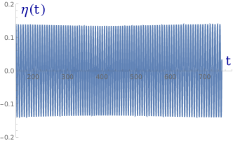
Figure 6: Left: trajectories of the vortex position $x(t)$ for the model with the second mode excited, for various values of the initial mode amplitude, and $v_{\rm in}=0.015$. Right: evolution of the mode amplitude $\eta(t)$ for the motion with the initial amplitude $\eta(0)=0.14$.

For head-on collisions we can consistently put $y=0$. Then the Lagrangian (93) reduces to

$$L=\frac{1}{2}\Omega(x){\dot{x}}^{2}+\frac{1}{2}{\dot{\eta}}^{2}-\frac{1}{2}\omega_{2}^{2}(x)\eta^{2}\,,$$ (94)

with

$$\omega_{2}^{2}(x)=\omega^{2}_{2}(0)-(\omega^{2}_{2}(0)-\omega^{2}_{2}(\infty))\left(1-e^{-0.2\sqrt{108}\,x}\right).$$ (95)

Because $\omega_{2}^{2}$ increases as $x$ decreases from a positive value and becomes negative, the inter-vortex force is always towards positive $x$, which has the following dynamical consequences for vortices approaching from $x=3$. If the initial amplitude of the second mode is sufficiently large, the vortices scatter back before coalescing, i.e. they do not reach $x=0$. With a smaller amplitude, they may pass through $x=0$ and reach a negative $x$ before scattering back, i.e. the vortices scatter from the horizontal to the vertical axis, stop and return to the horizontal axis. This is a 2-bounce solution. These possibilities are plotted in Fig. 6 where $v_{\rm in}=0.015$. If the amplitude is smaller still, the vortices separate sufficiently along the vertical axis that the third mode enters the continuum spectrum, and the so-called spectral wall phenomenon can be expected to occur [14]. This possibility is not taken into account in our collective coordinate model.

To conclude, from this adiabatic modelling we expect to observe at most 2-bounce scatterings of vortices in the full field theory dynamics when the second mode is initially excited, and we do not expect any chaotic multi-bounce pattern.

5 Outlook

In the present paper we proposed collective coordinate models for the dynamics of BPS 2-vortex solutions excited by their shape modes. The models generalize the standard geodesic flow on the 2-vortex moduli space ${\cal M}$ by including the shape mode amplitudes as additional collective coordinates. Importantly, in contrast to the force-free geodesic dynamics of unexcited BPS vortices, excitation of the shape modes introduces inter-vortex forces whose sign depends on how the relevant mode’s frequency varies over ${\cal M}$. This can significantly change the dynamics, leading to a complete breakdown of the original geodesic flow.

The most striking result is the appearance of a chaotic, probably self-similar, fractal-like pattern of multi-bounce windows in vortex-vortex collisions if the lowest shape mode is excited. This is explained in terms of the well-known resonant energy transfer mechanism. During collisions, the kinetic energy of vortex motion may be temporary transferred into shape mode energy. The vortices may then be unable to overcome the attractive interaction triggered by the mode excitation, and instead collide once again. This process repeats until the kinetic energy is again sufficiently large for the vortices to separate. A similar mechanism is very well understood in kink-antikink collisions in (1+1) dimensions, but here, for the first time, we have shown that it can also influence the dynamics of higher-dimensional solitons.

In particular, we have found that an even number of collisions (bounces) changes the famous $90^{\circ}$ scattering of vortices into $180^{\circ}$ backward scattering. Backward scattering can also occur if the higher-frequency (second) mode is excited, because in this case the excitation triggers a repulsive force between the vortices. Additionally, due to level crossing, this force becomes attractive after the vortices pass through the circularly symmetric configuration in a head-on collision (one bounce), which makes a second bounce more likely, resulting in backward scattering. No further bounces are possible in this channel.

Of course, all our predictions need to be verified by simulations of excited 2-vortex scattering in the full field theory [12]. We expect to find qualitative rather than quantitative agreement with the collective coordinate models, because the models make several simplifications which for a chaotic system may not be negligible. For example, we used simplified, analytical expressions for both the metric function and the dependence of the frequencies on the vortex separation. Also, we did not take into account a possible modification of the moduli space metric due to the amplitudes of the modes, even though it is known that vibrational (massive) degrees of freedom can affect the metric of kinetic, zero modes, see e.g. the description of a single, vibrating kink [10]. Such a metric modification is obviously a subleading effect in comparison with the appearance of an inter-vortex force, but nonetheless, it can affect the locations of bounce windows. Also, inclusion of non-quadratic terms in the effective potential may slightly change the dynamics.

Looking from a wider perspective, it is fascinating that effects previously associated only with one-dimensional kinks, find their counterparts in the dynamics of higher-dimensional solitons.

Appendix: Field theory derivation of the effective models

In this appendix, we sketch the derivation of the two effective models, identified in the main sections of this paper, governing the dynamics of BPS 2-vortices when shapes modes are excited. The Abelian Higgs field theory action is [15]

$$S=\int\left\{-\frac{1}{4}F_{\mu\nu}F^{\mu\nu}+\frac{1}{2}\overline{D_{\mu}\phi}\,D^{\mu}\phi-\frac{1}{8}(1-\bar{\phi}\phi)^{2}\right\}\,dx_{1}dx_{2}\,dt=\int\left\{T-V\right\}\,dt\,,$$ (96)

such that the kinetic and potential energy of the system in the temporal gauge $A_{0}=0$ are, respectively,

$$T=\frac{1}{2}\int\left\{\partial_{t}A_{i}\partial_{t}A_{i}+\partial_{t}\bar{\phi}\,\partial_{t}\phi\right\}\,dx_{1}dx_{2}\,,\quad V=\frac{1}{2}\int\left\{F_{ij}F_{ij}+\overline{D_{i}\phi}D_{i}\phi+\frac{1}{8}(1-\bar{\phi}\phi)^{2}\right\}\,dx_{1}dx_{2}\,.$$ (97)

It is well known that BPS 2-vortex solutions satisfy the first-order equations

$$F_{12}=\frac{1}{2}(1-\bar{\phi}\phi)\,,\quad D_{1}\phi+iD_{2}\phi=0\,,$$ (98)

and describe configurations where two unit magnetic flux vortices have an arbitrary separation. In the center of mass frame the 2-vortex solution is denoted as [6]

$$\widetilde{A}_{j}(X_{1},X_{2},x_{1},x_{2})\,,\quad\widetilde{\phi}(X_{1},X_{2},x_{1},x_{2})\,,$$ (99)

where $(X_{1},X_{2})$ are the spatial coordinates of a general point in the space-time. $\pm(x_{1},x_{2})$ specify the locations of the constituent vortices (zeros of the scalar field $\widetilde{\phi}$) and play the role of real coordinates on the centred 2-vortex moduli space ${\cal M}$. They can be combined into the complex coordinate $w=x_{1}+ix_{2}=\rho e^{i\theta}$ introduced in section 2, although as we have seen it is more convenient to work with a complex coordinate $z=x+iy=re^{i\varphi}$ proportional to $w^{2}$, that is, $z=kw^{2}$. Then $r=k\rho^{2}$ and $\varphi=2\theta$. Note that the angle $\theta$ varies only in the range $[-\frac{1}{2}\pi,\frac{1}{2}\pi]$ because adding $\pi$ moves the unit vortex at $(x_{1},x_{2})$ to $(-x_{1},-x_{2})$ and vice versa, but these two configurations are identical. On the other hand, $\varphi=2\theta$ has the normal angular range. In terms of the real moduli space coordinates $(x,y)$, the 2-vortex configurations (99) can be assembled as the column vector

$$\widetilde{\Phi}(X_{1},X_{2},x,y)=\left(\widetilde{A}_{1}(X_{1},X_{2},x,y),\widetilde{A}_{2}(X_{1},X_{2},x,y),\widetilde{\phi}_{1}(X_{1},X_{2},x,y),\widetilde{\phi}_{2}(X_{1},X_{2},x,y)\right)^{\rm T}\,,$$ (100)

where $\widetilde{\phi}_{1}$ and $\widetilde{\phi}_{2}$ are the real and imaginary parts of $\widetilde{\phi}$.

Collective coordinate model for 2-vortex dynamics with the lowest-frequency shape mode excited

The configuration for moving vortices with the lowest-frequency shape mode excited is written as

$$\widetilde{\Psi}(X_{1},X_{2},x(t),y(t))=\widetilde{\Phi}(X_{1},X_{2},x(t),y(t))+\eta(t)\,\xi_{1}(X_{1},X_{2},x(t),y(t))\,,$$ (101)

where $\xi_{1}$ denotes the lowest (normalized) shape mode of the second-order fluctuation operator ${\cal H}$,

$${\cal H}\,\xi_{1}(X_{1},X_{2},x,y)=\omega_{1}^{2}(r)\,\xi_{1}(X_{1},X_{2},x,y)\,,$$ (102)

and $\eta(t)$ is the real shape mode amplitude. Note that the frequency $\omega_{1}$ depends on the point in the moduli space where the spectral problem is studied, but because of rotational symmetry it only depends on $r=\sqrt{x^{2}+y^{2}}$. The flow over the moduli space of both the eigenfunction $\xi_{1}$ and the eigenvalue $\omega_{1}^{2}$ has been numerically described in [6]. $x$, $y$ and $\eta$ are the collective coordinates, whose effective dynamics is implemented by assuming that the temporal dependence of the fields in $\mathbb{R}^{2}$ is only through $\dot{x}$, $\dot{y}$ and $\dot{\eta}$. Under this hypothesis, the effective dynamical system is constructed as follows. Neglecting contributions of the form $\eta\int\dot{\widetilde{\Phi}}^{\rm T}\dot{\xi}_{1}\,dX_{1}dX_{2}$, $\eta\int\dot{\xi}_{1}^{\rm T}\dot{\widetilde{\Phi}}\,dX_{1}dX_{2}$ and $\eta^{2}\int\dot{\xi}_{1}^{\rm T}\dot{\xi}_{1}\,dX_{1}dX_{2}$, the effective kinetic energy reads

$$T_{\rm eff}=\frac{1}{2}g_{xx}(x,y)\dot{x}^{2}+\frac{1}{2}g_{yy}(x,y)\dot{y}^{2}+\frac{1}{2}\dot{\eta}^{2}\,,$$ (103)

where the metric factors are

$$g_{xx}(x,y)=\int\Big{(}\frac{\partial{\widetilde{\Phi}}}{\partial x}\Big{)}^{\rm T}\Big{(}\frac{\partial{\widetilde{\Phi}}}{\partial x}\Big{)}\,dX_{1}dX_{2}=\Omega(r)$$

$$g_{yy}(x,y)=\int\Big{(}\frac{\partial{\widetilde{\Phi}}}{\partial y}\Big{)}^{\rm T}\Big{(}\frac{\partial{\widetilde{\Phi}}}{\partial y}\Big{)}\,dX_{1}dX_{2}=\Omega(r)\,.$$ (104)

These integrals define the conformal factor $\Omega(r)$ of the Samols metric [7]. We finally obtain

$$T_{\rm eff}=\frac{1}{2}\Omega(r)\Big{(}\dot{x}^{2}+\dot{y}^{2}\Big{)}+\frac{1}{2}\dot{\eta}^{2}\,.$$ (105)

The contribution to the Lagrangian which does not depend on time derivatives is evaluated up to second-order in $\eta$, and is

$$\frac{1}{2}\eta^{2}\,\int\xi_{1}^{\rm T}(X_{1},X_{2},x,y)\,{\cal H}\,\xi_{1}(X_{1},X_{2},x,y)\,dX_{1}dX_{2}\,.$$ (106)

Using (102) and taking into account the rotational symmetry, we find the effective potential over the moduli space,

$$V_{\rm eff}(x,y,\eta)=\frac{1}{2}\omega_{1}^{2}(r)\eta^{2}\,.$$ (107)

Because $\omega_{1}^{2}(r)$ has its minimum value $\omega_{1}^{2}(0)$ at the origin and increases to a finite value $\omega_{1}^{2}(\infty)>\omega_{1}^{2}(0)$ at infinity, attractive forces arise between the vortices when the lowest shape mode is excited. Moreover, this potential is proportional to the squared amplitude of the mode, opening the door to transfer of energy from the mode into the kinetic energy of vortices moving through the moduli space. Thus, the effective Lagrangian

$$L_{\rm eff}=T_{\rm eff}-V_{\rm eff}=\frac{1}{2}\Omega(r)\Big{(}\dot{x}^{2}+\dot{y}^{2}\Big{)}+\frac{1}{2}\dot{\eta}^{2}-\frac{1}{2}\omega_{1}^{2}(r)\eta^{2}\,,$$ (108)

the starting point of section 3, is obtained from the field theory as an effective collective coordinate model. We stress finally that incorporating the effect of the shape mode up to second-order generalizes to the quantized theory as a 1-loop/semi-classical correction to moduli space dynamics.

Collective coordinate model for 2-vortex dynamics with the two higher-frequency shape modes excited

Consider the configuration

$$\Sigma(X_{1},X_{2},x(t),y(t))=\widetilde{\Phi}(X_{1},X_{2},x(t),y(t))+\eta_{2}(t)\,\xi_{2}(X_{1},X_{2},x(t),y(t))+\eta_{3}(t)\,\xi_{3}(X_{1},X_{2},x(t),y(t))\,,$$ (109)

which describes a dynamical 2-vortex excited by the shape modes $\xi_{2}$ and $\xi_{3}$ having the higher frequencies $\omega_{2}$ and $\omega_{3}\geq\omega_{2}$, respectively, and amplitudes $\eta_{2}$ and $\eta_{3}$. These modes are mutually orthogonal eigenfunctions of the second-order fluctuation operator ${\cal H}$, see [6],

$${\cal H}\,\xi_{i}(X_{1},X_{2},x,y)=\omega_{i}^{2}(r)\,\xi_{i}(X_{1},X_{2},x,y)\,,\hskip 8.5359pti=2,3\,.$$ (110)

The spectral flow of $\omega_{2}^{2}$ and $\omega_{3}^{2}$ over ${\cal M}$ is summarized as follows:

• The frequencies are rotationally symmetric over ${\cal M}$ and only depend on $r$.

• At the apex of ${\cal M}$, the two frequencies degenerate: $\omega_{2}^{2}(0)=\omega_{3}^{2}(0)$.

• $\omega_{2}^{2}(r)$ decreases linearly with $r$ near $r=0$, and approaches the limit $\omega_{2}^{2}(\infty)=\omega_{1}^{2}(\infty)>0$.

• $\omega_{3}^{2}(r)$ increases linearly with $r$ near $r=0$, reaching 1 at the boundary of a disc in ${\cal M}$ where the mode $\xi_{3}$ disappears into the continuum.

Arguing exactly as in the previous derivation of the effective model for the lower-frequency shape mode we envisage the following effective Lagrangian for the upper-frequency modes:

$$L_{\rm eff}=\frac{1}{2}\Omega(r)(\dot{x}^{2}+\dot{y}^{2})+\frac{1}{2}\dot{\eta}_{2}^{2}+\frac{1}{2}\dot{\eta}_{3}^{2}-\frac{1}{2}\omega_{2}^{2}(r)\eta_{2}^{2}-\frac{1}{2}\omega_{3}^{2}(r)\eta_{3}^{2}\,.$$ (111)

Investigation of the effective dynamics including the higher-frequency modes is particularly worthwhile inside the disc where both modes are present. Here, one can approximate any BPS 2-vortex solution by adding a zero mode of suitable amplitude to the circularly-symmetric, coincident 2-vortex solution. This produces a splitting of the double zero of the Higgs field into two single zeros with a small separation $2\rho$. The collective coordinate procedure prescribes that the motion through ${\cal M}$ is only due to the time-dependence of $\rho(t)$. If the shape modes of frequencies $\omega_{2}$ and $\omega_{3}$ are also excited, we are led to study the effective dynamics of the configurations

$$\Sigma(X_{1},X_{2},x(t),y(t)) = \widetilde{\Phi}(X_{1},X_{2},0,0)+\epsilon(t)\,\xi_{0}(X_{1},X_{2},0,0))$$ (112)

$$\qquad+\eta_{2}(t)\,\xi_{2}(X_{1},X_{2},0,0)+\eta_{3}(t)\,\xi_{3}(X_{1},X_{2},0,0)\,.$$

$\epsilon$, $\eta_{2}$ and $\eta_{3}$ are, respectively, the amplitudes of the zero mode and these two shape modes, the new collective coordinates. Plugging the expression (112) into the second-order action we obtain

$$S^{(2)}=\frac{1}{2}\int\Big{\{}\|\xi_{0}\|^{2}{\dot{\epsilon}}^{2}(t)+\|\xi_{2}\|^{2}{\dot{\eta}}^{2}_{2}(t)+\|\xi_{3}\|^{2}{\dot{\eta}}^{2}_{3}(t)-\omega_{2}^{2}(r)\|\xi_{2}\|^{2}\eta_{2}^{2}(t)-\omega_{3}^{2}(r)\|\xi_{3}\|^{2}\eta_{3}^{2}(t)\Big{\}}\,dt\,,$$ (113)

where the orthogonality of the eigenfunctions $\xi_{i}$ of ${\cal H}$ has been employed. We can assume that the shape modes $\xi_{2}$ and $\xi_{3}$ are normalized, but we shall use the non-normalized zero mode

$$\xi_{0}(X_{1},X_{2},0,0)=R\left(h(R)\sin\Theta\,,h(R)\cos\Theta\,,-\frac{h^{\prime}(R)}{f_{2}(R)}\,,\,0\right)^{\rm T}$$ (114)

described in [5, 6], where $(R,\Theta)$ here denote spatial polar coordinates, i.e. $X_{1}=R\cos\Theta$ and $X_{2}=R\sin\Theta$. This choice of the zero mode involves the splitting of the vortex zeros in the $x_{2}$-direction (vertical direction) away from the apex of the moduli space, such that $x_{2}(t)$ determines the inter-vortex distance. The expression (114) allows us to find a relation between the amplitude $\epsilon$ of the zero mode $\xi_{0}$ and $x_{2}$ as

$$\epsilon(t)=\frac{(\delta_{2})^{2}}{2|c_{2}|}\,(x_{2}(t))^{2}=C_{1}\,(x_{2}(t))^{2}=\frac{C_{1}}{k}\,r(t)$$ (115)

where $\delta_{2}\approx 0.236146$ and $c_{2}\approx-0.277308$. These values come from the local behaviour of the coincident 2-vortex Higgs field profile $f_{2}(R)\approx\delta_{2}R^{2}$ and of the zero mode (114) with $h(R)\approx 1+c_{2}R^{2}$. Additionally,

$$\omega_{2}^{2}(r)=\lambda-\frac{C_{2}}{k}\,r\,,\hskip 14.22636pt\omega_{3}^{2}(r)=\lambda+\frac{C_{2}}{k}\,r$$ (116)

where $\lambda=\omega_{2}^{2}(0)=\omega_{3}^{2}(0)\approx 0.97303$ and $C_{2}\approx 0.025873$. Working with the expressions (115) and (116), the action becomes

$$S^{(2)}=\frac{1}{2}\int\Bigg{\{}\frac{C_{1}^{2}}{k^{2}}\|\xi_{0}\|^{2}\,\dot{r}^{2}(t)+\dot{\eta}_{2}^{2}(t)+\dot{\eta}_{3}^{2}(t)-\left(\lambda-\frac{C_{2}}{k}\,r(t)\right)\,\eta_{2}^{2}(t)-\left(\lambda+\frac{C_{2}}{k}r(t)\right)\,\eta_{3}^{2}(t)\Bigg{\}}\,dt\,,$$ (117)

with $\|\xi_{0}\|^{2}\approx 62.4936$. We now combine the two real shape mode amplitudes into a single complex amplitude $\chi$,

$$\eta_{3}=\frac{1}{\sqrt{2}}\left(e^{\frac{i}{2}\varphi}\chi^{*}+e^{-\frac{i}{2}\varphi}\chi\right)=\eta^{*}_{3}\,,\quad\eta_{2}=\frac{1}{\sqrt{2}\,i}\left(e^{\frac{i}{2}\varphi}\chi^{*}-e^{-\frac{i}{2}\varphi}\chi\right)=\eta^{*}_{2}\,,$$ (118)

which involves the argument $\varphi$ of the coordinate $z=re^{i\varphi}$ on the moduli space. This induces a rotation which generalizes the dynamics. Now the motion can be in any direction through the origin of the moduli space, and the Lagrangian in (117) becomes

$$L_{\rm eff}=\frac{1}{2}\frac{C_{1}^{2}}{k^{2}}\|\xi_{0}\|^{2}\,\dot{z}^{*}\dot{z}+\dot{\chi}^{*}\dot{\chi}-\lambda\chi^{*}\chi-\frac{1}{2}\frac{C_{2}}{k}z^{*}\chi^{2}-\frac{1}{2}\frac{C_{2}}{k}z\chi^{*2}\,.$$ (119)

Finally, if the value of $k$ is set as $k=C_{1}\|\xi_{0}\|$ and we define $\alpha=C_{2}/(C_{1}\|\xi_{0}\|)$ then the effective Lagrangian becomes

$$L_{\rm eff}=\frac{1}{2}\,\dot{z}^{*}\dot{z}+\dot{\chi}^{*}\dot{\chi}-\lambda\chi^{*}\chi-\frac{1}{2}\alpha z^{*}\chi^{2}-\frac{1}{2}\alpha z\chi^{*2}\,,$$ (120)

which reproduces the expression (63) introduced in the main text.

References

- [1]
- [2] H. Arodź, Bound states of the vector field with a vortex in the Abelian Higgs model, Acta Phys. Pol. B22, 511 (1991).
- [3] M. Goodband and M. Hindmarsh, Bound states and instabilities of vortices, Phys. Rev. D52, 4621 (1995).
- [4] A. Alonso-Izquierdo, W. Garcia Fuertes and J. Mateos Guilarte, A note on BPS vortex bound states, Phys. Lett. B753, 29 (2016).
- [5] A. Alonso Izquierdo, W. Garcia Fuertes and J. Mateos Guilarte, Dissecting zero modes and bound states on BPS vortices in Ginzburg–Landau superconductors, J. High Energy Phys. 05 (2016) 074.
- [6] A. Alonso Izquierdo, W. Garcia Fuertes, N. S. Manton and J. Mateos Guilarte, Spectral flow of vortex shape modes over the BPS 2-vortex moduli space, J. High Energy Phys. 01 (2024) 020.
- [7] T. M. Samols, Vortex scattering, Commun. Math. Phys. 145, 149 (1992).
- [8] T. Sugiyama, Kink-antikink collisions in the two-dimensional model, Prog. Theor. Phys. 61, 1550 (1979).
- [9] D. K. Campbell, J. F. Schonfeld and C. A. Wingate, Resonance structure in kink-antikink interactions in theory, Physica D 9, 1 (1983).
- [10] N. S. Manton, K. Oles, T. Romanczukiewicz and A. Wereszczynski, Collective coordinate model of kink-antikink collisions in theory, Phys. Rev. Lett. 127, 071601 (2021).
- [11] N. S. Manton and J. M. Speight, Asymptotic interactions of critically coupled vortices, Commun. Math. Phys. 236, 535 (2003).
- [12] S. Krusch, M. Rees and T. Winyard, work in preparation.
- [13] A. Alonso Izquierdo, L. M. Nieto, J. Queiroga-Nunes, Scattering between wobbling kinks, Phys. Rev. D103, 045003 (2021).
- [14] C. Adam, K. Oles, T. Romanczukiewicz and A. Wereszczynski, Spectral walls in soliton collisions, Phys. Rev. Lett. 122, 241601 (2019).
- [15] N. Manton and P. Sutcliffe, Topological Solitons, Cambridge University Press, Cambridge, 2004.