MANTA: A Negative-Triangularity NASEM-Compliant Fusion Pilot Plant

Abstract

The MANTA (Modular Adjustable Negative Triangularity ARC-class) design study investigated how negative-triangularity (NT) may be leveraged in a compact, fusion pilot plant (FPP) to take a “power-handling first” approach. The result is a pulsed, radiative, ELM-free tokamak that satisfies and exceeds the FPP requirements described in the 2021 National Academies of Sciences, Engineering, and Medicine report “Bringing Fusion to the U.S. Grid”[1]. A self-consistent integrated modeling workflow predicts a fusion power of 450 MW and a plasma gain of 11.5 with only 23.5 MW of power to the scrape-off layer (SOL). This low $P_{\text{SOL}}$ together with impurity seeding and high density at the separatrix results in a peak heat flux of just 2.8 MW/m². MANTA’s high aspect ratio provides space for a large central solenoid (CS), resulting in ${\sim}$15 minute inductive pulses. In spite of the high B fields on the CS and the other REBCO-based magnets, the electromagnetic stresses remain below structural and critical current density limits. Iterative optimization of neutron shielding and tritium breeding blanket yield tritium self-sufficiency with a breeding ratio of 1.15, a blanket power multiplication factor of 1.11, toroidal field coil lifetimes of $3100\pm 400$ MW-yr, and poloidal field coil lifetimes of at least $890\pm 40$ MW-yr. Following balance of plant modeling, MANTA is projected to generate 90 MW of net electricity at an electricity gain factor of ${\sim}2.4$. Systems-level economic analysis estimates an overnight cost of US$3.4 billion, meeting the NASEM FPP requirement that this first-of-a-kind be less than US$5 billion. The toroidal field coil cost and replacement time are the most critical upfront and lifetime cost drivers, respectively.

1 Introduction and Overview

For fusion energy to contribute towards achieving decarbonization targets, a fusion pilot plant (FPP) must begin operation in the 2030s. Scoping an FPP must therefore begin now, [1] and its design must provide cost and operational certainty for fusion energy commercialization. A significant challenge in scaling the tokamak concept, and more generally magnetic fusion, to an FPP is maintaining a high performance core plasma with peak heat fluxes to the plasma facing components (PFCs) within technological limits for heat removal. And this must be achieved simultaneously with the high average power desired for commercial fusion devices. Exceeding this heat removal limit would result in component failure and a maintenance period for replacement. Furthermore, erosion of PFCs occurs even in modern devices[2, 3], where discharges durations and steady-state heat flux fluxes are, respectively, ${\sim}2$ and ${\sim}1$ orders of magnitude below that expected for reactors[4, 5, 6]. FPPs and commercial fusion devices will therefore require a dissipative divertor, where a significant amount of power is radiated between the separatrix and the divertor targets, and overall a reliable and robust strategy to dissipate fusion plasma power to the PFCs.

Typical H-mode operation results in an additional transient heat flux in the form of edge-localized modes (ELMs)[5, 6]. These bursts of particles and energy through the SOL pose a significant risk to PFCs, and their severity increases with the stored energy of the plasma[7]. Proposed devices such as EU-DEMO will be unable to operate without ELM control[8]. While ELM-free regimes do exist, the ability to concurrently achieve high performance, ELM mitigation, and a dissipative divertor is often restricted to subsets parameter space, which may not be compatible with the requirements of a power plant[9, 10].

A potential solution is the use of negative triangularity ($\delta<0$), where the plasma’s D-shaped cross section is inverted relative to the usual positive triangularity. The triangularity $\delta$ is taken to be the average up the upper and lower triangularities $\delta_{u,l}=(R_{\text{geo}}-R_{u,l})/a$, where $R_{\text{geo}}$ is the geometrical major radius, $R_{\text{u,l}}$ is the major radius of the highest/lowest point on the last closed flux surface (LCFS), and $a$ is the minor radius[11]. A comparison between a positive and negative triangularity plasma with otherwise identical shaping parameters is given in Fig 1. With sufficiently negative triangularity (NT), the 2nd stability region for infinite-n ballooning modes is inaccessible[12, 13]. This prevents the plasma from entering H-mode and developing the steep edge gradients that produce ELMs. There is also then no requirement of a minimum SOL power as there is in H-mode. This permits a higher fraction of the total power to be radiated from the core, reducing the power incident on the divertor targets. Additional power-handling benefits are detailed in Section 3. It is important to note that even without H-mode, the use of NT does not preclude high fusion performance, as will be discussed in Section 2.

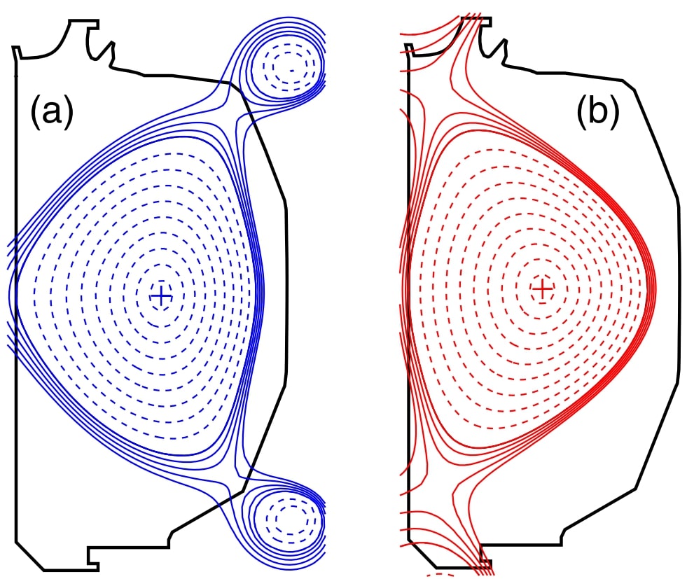
Figure 1: Comparison of the plasma cross sections for negative (a) and positive (b) triangularities on the DIII-D tokamak. Figure reproduced from [14] with the permission of the American Physical Society.

Application of NT to power-plant scale tokamaks has been explored in several previous works[15, 16, 17, 18]. This paper builds on previous studies but differs in two major ways. First, all magnets are assumed to be constructed from Rare-Earth Barium Copper Oxide (REBCO) high-temperature superconductors (HTS), opening portions of parameter space not previously investigated for NT designs. Second, an integrated reactor design is presented, in which core transport, power-handling, magnet systems, neutronics, and economic viability were simultaneously optimized to inform the overall design.

The result of this study is MANTA (Modular Adjustable Negative-Triangularity ARC-class): a pulsed, radiative, ELM-free, negative triangularity ARC-class[19] tokamak FPP. MANTA’s design is shown in Fig 2 and was developed with a focus on maximizing self-consistency. MANTA advances the three scientific and technological readiness drivers outlined in the Fusion Energy Sciences Advisory Committee’s “Powering the Future Fusion & Plasmas” report[20]: sustaining a burning plasma, engineering for extreme conditions, and harnessing fusion energy. MANTA also surpasses the criteria to demonstrate the path to commercial viability of nuclear fusion energy as laid out in the National Academies of Sciences, Engineering, and Medicine (NASEM) “Bringing Fusion to the U.S. Grid” report[1], namely:

1. Electricity gain factor: $Q_{\text{e}}>1$

2. Continuous net electricity $\geq$ 50 MWe for at least 3 hours

3. Tritium Breeding Ratio (TBR) $\gtrsim$ 0.9

4. Overnight cost $<$ US$\$5$B

5. Operation through several environmental cycles

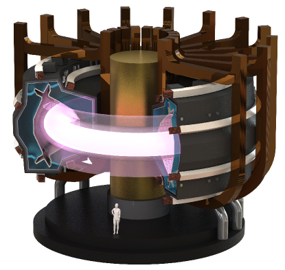
Figure 2: MANTA is a compact, negative triangularity fusion pilot plant. An average sized human adult is present for scale.

It is worth emphasizing that MANTA is not a commercial power plant, but rather a pilot plant. Maximizing absolute performance was therefore not the goal of this study. Instead, a focus was placed on maintainability and flexibility at the conditions relevant to a power plant. Further optimizations may be possible, but MANTA is well-suited to its role as a pilot plant and both fulfills the NASEM requirements and advances the FESAC goals.

Namely, MANTA’s modularity and rapid maintenance permits faster advancement of fusion science and technology. This is achieved through a liquid immersion FLiBe tank that permits modifications to the vacuum vessel (VV) without requiring changes to the blanket system and demountable toroidal field (TF) coils that give ready access to the FLiBe tank and VV. The TF coils may be ramped relatively quickly due to an oversized cryosystem, and replacement of the FLiBe tank and VV as a single assembly reduces radiation hazards and speeds maintenance.

Additionally, while only a single operating point was investigated with integrated modeling, 0D scoping predicts adjustable fusion power with near constant $P_{\text{SOL}}$ through control of the density. This allows for the testing of physics and technology over a range of conditions without worsening the power-handling challenge.

Table 1: MANTA Key Design Parameters

Parameter	Symbol	Value
Fusion power	$P_{\text{fus}}$	450 MW
Total thermal power	$P_{\rm th}$	530 MW
Net electric power	$P_{\rm e,net}$	90 MWe
ICRF coupled power	$P_{\rm ICRH}$	40 MW
Scrape-off layer power	$P_{\text{SOL}}$	23.5 MW
Plasma gain	$Q$	11.5
Electricity gain	$Q_{E}$	2.4
Major radius	$R_{0}$	4.55 m
Plasma minor radius	a	1.2 m
Plasma elongation	$\kappa$	1.4
Plasma triangularity	$\delta$	-0.5
Plasma volume	$V_{p}$	155 $m^{3}$
Plasma surface area	$A_{p}$	258 $m^{2}$
Toroidal magnetic field	$B_{0}$	11 T
Plasma current	$I_{P}$	10 MA
Bootstrap fraction	$f_{\rm BS}$	18%
Tritium breeding ratio	TBR	1.15
Avg. ion temperature	〈$T_{i}$〉	7.3 keV
Avg. electron temperature	〈$T_{e}$〉	7.1 keV
Avg. density	〈n〉	1.95$\cdot 10^{20}$ m-3
On-axis ion temperature	$T_{i,0}$	19 keV
On-axis e- temperature	$T_{e,0}$	18.8 keV
On-axis e- density	$n_{0}$	2.76$\cdot 10^{20}$ m-3
Greenwald fraction	$f_{\rm Gr}$	0.88
Pulse length	$\tau_{\rm pulse}$	15 min
Inter-pulse length	$\tau_{\rm inter}$	2 min
Normalized beta	$\beta_{N}$	1.35
Safety factor at $\Psi_{N}$ = 0.95	$q_{95}$	2.3
Minimum safety factor	$q_{\rm min}$	0.905
Energy confinement time	$\tau_{E}$	0.94 s
H89 confinement factor	H89	1.44
Loop voltage	V${}_{\text{loop}}$	0.206 V

A list of MANTA’s key parameters at its design point is given in Table 1. The remainder of the paper consists of the following sections: Sec. 2 scopes MANTA’s fusion core solution via 0-D power balance before refining the operating point with an integrated modeling workflow; Sec. 3 develops a power-handling solution capable of withstanding the exhausted and radiated power determined by the core modeling; Sec. 4 details the design, mechanical analysis, and maintenance of the toroidal field (TF) coils, central solenoid (CS), and poloidal field (PF) coils; Sec. 5 uses neutronics simulations to calculate magnet lifetimes and analyze the tritium fuel cycle; Sec. 6 discusses MANTA’s balance of plant and determines the steady state net electrical power; Sec. 7 provides an economic analysis of MANTA to investigate its financing; and Sec. 8 gives concluding remarks.

2 Plasma Core

In addition to its advantages in power-handling, negative triangularity also improves core performance with some NT plasmas on DIII-D and TCV achieving H-mode-level confinement (H₉₈ = 1).[14, 21, 22, 23, 24] This is made possible by NT’s weaker power degradation of the energy confinement time and a reduction in the electron heat transport.[22, 25, 23, 26] Importantly, high performance dimensionless parameters of $\beta_{N}>3$, $f_{Gr}>1$, and $q_{95}<3$ have been achieved simultaneously in a diverted configuration with this high confinement of $H_{98}>1$[24], where $f_{Gr}$ is the Greenwald fraction, $\beta_{N}$ is the normalized $\beta$, and $q_{95}$ is the safety factor at $\psi_{N}=0.95$. These promising results warrant the investigation of NT FPP designs, like MANTA, despite NT being far less explored than PT.

2.1 0-D Scoping of the Core Solution

Broad scoping of the space of core solutions capable of meeting the NASEM requirements was completed through the use of POPCONs (Plasma OPerational CONtours), 0-D models of tokamak core performance that solve the global power-balance equation [27]. MANTA’s POPCONs were generated with the open source code CFSpopcon [28]. Key POPCON outputs include fusion power $P_{\mathrm{fus}}$, required auxiliary heating power $P_{\rm aux}$, radiated power $P_{\rm rad}$, and plasma gain $Q_{p}$, all of which were calculated over a range of volume-averaged $T_{e}$ and $n_{e}$ values. The temperature and density profiles were taken as user-inputs. Krypton was chosen as the core radiator to achieve the necessary radiated power, primarily in the outer parts of the core plasma, to maintain low $P_{\mathrm{SOL}}$. The krypton density profile was assumed to be a scaled version of the electron density profile. It was additionally assumed that the radiative power fractions viable in PT L-mode[29] were also acceptable for ELM-free NT. Uncertain parameters, such as the confinement factor or profile shaping parameters were varied over conservative ranges from the literature. Historical PT L-mode data [30] was used as reference for density peaking, while the recent DIII-D NT campaign [24] informed the choice of H98y2 energy confinement scalings [31].

Additional free parameters included the triangularity $\delta$, the elongation $\kappa$, the minor radius $a$, the major radius $R_{0}$, the toroidal magnetic field $B_{T}$, and the plasma current $I_{p}$. To ensure the second stability region for infinite-n ballooning modes and hence H-mode was inaccessible regardless of the choice of other parameters, a highly negative triangularity of $\delta=-0.5$ was selected. $B_{T}$ on axis was assumed to be 11 T as this is broadly consistent with the magnetic field in other high-field tokamak designs, such as SPARC[32], which have completed extensive magnet analyses. $I_{p}$ was chosen to be driven inductively to avoid the cost and complexity of a non-inductive current drive system. This leads to a preference for larger aspect ratios as the wider inner bore fits a larger central solenoid capable of a greater flux swing. An increased magnetic flux extends the duration of flattop operation, aiding MANTA’s ability to meet the fusion power duration requirement.

To satisfy the NASEM requirement of 50 MWe net electric power, the minimum $P_{\mathrm{fus}}$ was initially estimated to be $200$ MW (though this would later prove to be too low), with higher $P_{\mathrm{fus}}$ desirable within the constraints of component lifetimes and economics. $P_{\mathrm{fus}}$ increases with larger $I_{p}$ due to the longer confinement time[31] and with $R_{0}$, $a$, and $\kappa$ due to both increases in the confinement time and also the larger plasma volume: $V_{\text{p}}\approx 2\pi^{2}R_{0}a^{2}\kappa$. $I_{p}$ is constrained by the increased risk of kink instability at large currents. To account for this, $I_{p}$ was removed as a free parameter and replaced by a target kink safety-factor $q_{*}\approx 2.5$, well above the marginal kink safety factor $q_{\star}=2$ reported in [33]. $I_{p}$ was then calculated from $q_{*}$ as per [33]:

$$I_{p}=\frac{2\pi a^{2}B_{0}}{\mu_{0}R_{0}q_{*}}\Bigl{(}\frac{1+\kappa^{2}}{2}\Bigr{)}10^{-6}\text{ [MA]}.$$ (1)

$\kappa$ was constrained by the increased risk of vertical displacements at high $\kappa$[34], an effect exacerbated by NT[35]. To balance plasma volume and stability, $\kappa=1.4$ was selected based on results from the AVSTAB vertical stability model [35, 36]. The use of passive stability plates may allow for access to higher elongations[37], but this was not explored for MANTA’s design and could be an area of future work.

$R_{0}$ and $a$ were constrained by the expense of the toroidal field magnets (which scales with the plasma surface area $\approx 2\pi^{2}R_{0}a(1+\kappa)$) and by component lifetimes. Using the Monte Carlo code OpenMC[38], neutronics simulations of some POPCON solutions were completed. The magnetic equilibria of these cases were computed by the Grad-Shafranov solver CHEASE [39] and were to assumed to be up-down symmetric double nulls. Such an equilibrium both aids in power-handling and simplifies MANTA’s design. From these simulations and economic calculations, $R_{0}=4.55$ and $a=1.2$ were selected to balance performance, component lifetime, and device cost. $I_{p}$ was then set at $10$  MA, resulting in $q_{\star}=2.59$. It is important to note that the avoidance of tearing modes was not factored into parameter selection and could be an area of future work.

The POPCON for this scenario is given in Fig. 3, where MANTA’s operating point is marked by the white circle, and the density and temperature profiles are those calculated by the transport code TGYRO [40], detailed below. Notably, this POPCON features near vertical contours of $P_{\mathrm{SOL}}$ near the chosen operating point. A range of $P_{\mathrm{fus}}$ values can therefore be achieved with near constant $P_{\mathrm{SOL}}$ through controlling the density. This adjustability permits the potential study of multiple operating points without largely affecting the divertor power handling solution. And the choice of an inductive plasma means these changes in density affect the pulse length, rather than the ability to drive the required current, as would be the case in a non-inductive plasma.

An ion cyclotron range of frequencies (ICRF) minority heating [41] system was selected to supply the required 40 MW of auxiliary power for this operating point due the efficient bulk core heating such a system provides. Mirroring SPARC [42], $\rm{}^{3}He$ was chosen as the minority species, which takes advantage of the overlap between the fundamental and second harmonic resonances of $\rm{}^{3}He$ and tritium, respectively. A minority fraction of $f_{\mathrm{He3}}=n_{\mathrm{He3}}/n_{\mathrm{e}}=2.5$% was taken to maintain good wave polarization with dilution away from the optimal 50/50 D-T ratio. The launched parallel refractive index $N_{\parallel}$ was chosen to be similar to SPARC [42], resulting in a toroidal refractive index $N_{\phi}=30$. On-axis damping corresponded to a frequency of 110 MHz, readily achievable by existing high power tetrodes [43]. While a detailed antenna design is outside the scope of this study, it should be noted that NT places the broad side of the plasma on the outboard wall, giving a large, relatively flat area suitable to a variety of antenna configurations.

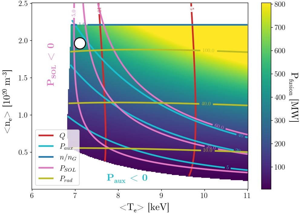
Figure 3: POPCON analysis of the parameter space around MANTA’s operating point. The chosen operating point is marked with a white circle, and the possible operating space is the colored region. At higher densities, the Greenwald density limit is exceeded. Lower temperatures and densities result in non-physical solutions. The profiles and confinement used in this POPCON matched those from the STEP modeling detailed in Sec. 2.2.

2.2 Plasma Core Integrated Workflow

Following selection of MANTA’s 0-D parameters from the POPCON scoping, an integrated workflow was employed to obtain a more realistic and self-consistent core solution. This workflow, illustrated in Fig. 4, linked multiple high-fidelity codes to map plasma parameters from the core to the divertor targets. This was made possible in part by the OMFIT STEP module [44], which allows self-consistent iteration between equilibrium, heating, transport, and stability codes in the OMFIT framework [45]. STEP accomplishes this via the OMAS (Ordered Multidimensional Array Structure) data structure to automatically transfer the outputs of one OMFIT module as inputs of the next.

The codes used in this workflow and their functions are as follows: CHEASE[39] is a fixed-boundary Grad-Shafranov solver that produced MHD magnetic equilibria; PRO-create[46] generated plasma profiles from 0D parameters; BALOO[47] calculated the ballooning stability of the edge pressure gradient; TORIC[48] is a full-wave solver that determined the electromagnetic fields resulting from the ICRF system; CQL3D[49] is a Fokker-Plank code that evolved the distribution functions of the chosen species, in this case due to the RF; CHEF[50] runs multiple heating and current drive codes to predict steady-state power deposition and current density profiles; TGYRO[40] is a transport code that evolved plasma profiles such that collision and transport losses balance the input power; The neoclassical transport code NEO [51] calculated these collisional losses, and the quasilinear turbulent transport code TGLF [52] calculated the transport losses; and UEDGE is a 2D edge transport code that extended plasma profiles to the divertor targets (see Section 3). Throughout this workflow, density profiles were held fixed with a peaking value given by the Angioni scaling[53]. This was done primarily to simplify flux matching performed by TGLF by excluding particle flux, and it is of note that particle sources in a reactor are expected to be localized outside of $\rho=0.95$ and TGLF has shown significant variability in density peaking prediction[54]. Allowing density to also evolve may be investigated in future work.

The difficulty in maintaining self-consistency throughout this workflow is that all of the codes are functions of the plasma profiles, but these profiles are the result of running all of the codes. For this reason, the workflow was completed twice. The first iteration began with passing CHEASE’s magnetic equilibrium (generated for the POPCON scans) to STEP. Density and temperature profiles were then initialized in PRO-create[46] based on the core temperature and density predicted by the POPCON analysis under the constraint of edge conditions (from BALOO [47]) feasible for a ballooning stable NT edge. Using these density and temperature profiles, an updated equilibrium was generated. The new CHEASE equilibrium, PRO-create plasma profiles, and CHEF heating sources were then fed into TGYRO, which evolved the electron and ion temperature profiles. TGYRO and CHEASE were iterated between until convergence was reached. An in-depth description of the TGYRO transport simulations and PRO-create profile generation is given in subsection 2.2.2.

The second iteration passed the TGYRO temperature profiles and the PRO-create density profiles to TORIC/CQL3D (further described in Section 2.2.1) to generate more accurate auxiliary heating profiles for the bulk ions and electrons. These heating profiles were copied into CHEF and updated temperature profiles were calculated by TGYRO. Again TGYRO was iterated with CHEASE until convergence. The profiles resulting from this workflow were then passed to UEDGE to extend the solution from the separatrix to the divertor targets (see Sec. 3). Future work could entail further iterations of this workflow to improve self-consistency.

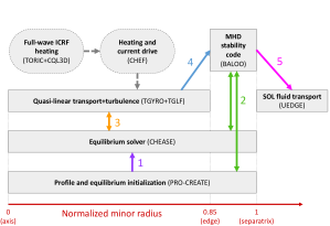
Figure 4: Integrated workflow schematic showing the codes used to simulate the various regions of the plasma and the iteration between these codes.

2.2.1 RF Power Deposition Profiles from TORIC/CQL3D

The full-wave code TORIC [48] solved Maxwell’s equations to calculate the electric fields generated by the ICRF system and obtain the RF power deposition profiles for D, T, $\rm{}^{3}He$, Kr, and electrons. The resulting electric field and power deposition cross sections are shown in Fig. 5. (a) and (b) show the two circularly polarized electric field component magnitudes. The choice of $f_{\mathrm{He3}}=2.5$% resulted in a large value of $E_{+}$ at the fundamental $\rm{}^{3}He$ resonance, producing strong local heating of up to 20 MW/m³, as shown in (c). Being collocated at this region of large $E_{+}$, the next strongest heating is 2nd harmonic tritium, shown in (d). Electron heating due to the fast wave and the ion Bernstein wave (IBW), shown in (e) and (f), are relatively small. Heating of D and Kr were found to be negligible and are not shown.

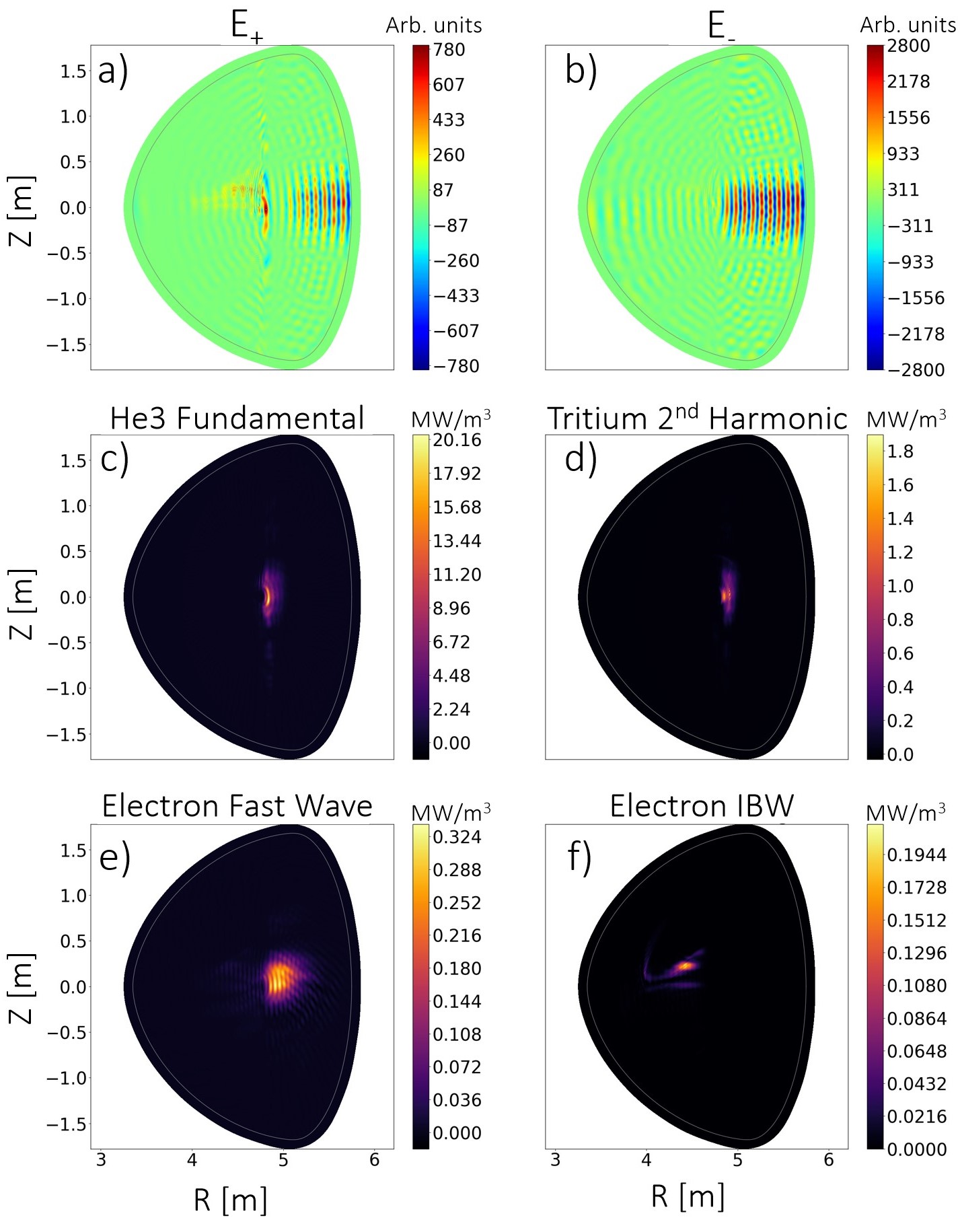
Figure 5: The electric field and RF power deposition calculated by TORIC/CQL3D. There is little direct absorption of the RF power by the electrons. (a) and (b) show the two circularly polarized electric field components ($E_{||}$ is small and is not shown). (c) and (d) show the RF power deposition for the $\rm{}^{3}He$ minority and T, respectively. (e) and (f) show the RF power deposition for the the electrons due the fast wave and the ion Bernstein wave, respectively.

The Fokker-Planck code CQL3D[49] was then coupled[55] to TORIC to determine how the energy deposited on the minority ions was partitioned to the bulk ions and electrons via Coulomb collisions. The two codes were iterated 100 times with good convergence. The resulting 1D power deposition profiles calculated by TORIC/CQL3D (shown in Figure 7 as $Q_{\text{e, aux}}$ and $Q_{\text{i, aux}}$) were then passed to CHEF for easy integration into STEP for the second iteration of TGYRO.

2.2.2 Transport Simulation with TGYRO in STEP

Transport modeling was completed with TGYRO, which modified the temperature profiles such that the collision and transport losses, calculated respectively by the neoclassical transport code NEO [51] and the quasilinear turbulent transport code TGLF [52], balance the input power. TGLF was run with saturation rule SAT-2[56, 57], as this produces profiles that are in good agreement with DIII-D NT experiments [58] and has been used in similar conceptual design studies[29]. Species included in the simulation were electrons, D, T, and Kr. Notably, $2.5\%$ ³He and ${\sim}2\%$ ⁴He were not included and could be an area of future research. Bremsstrahlung and synchotron radiation are included. Temperature profiles with various core and edge values were converged until a solution was found with acceptable scrape-off-layer power $P_{\text{SOL}}$, radiative fraction $f_{\text{rad}}$, fusion power $P_{\text{fus}}$, and Greenwald faction $f_{\text{Gr}}$.

Free variables for STEP profile optimization were electron density at the boundary of TGYRO evolution ($\rho=0.85$) $n_{85}$, Kr concentration $f_{\text{Kr}}$, and temperature at $\rho=0.85$ $T_{85}$. D and T density profiles were generated by PRO-create assuming a 50/50 mix and enforcing quasineutrality given the electron and Kr density profiles. The Kr density profile was assumed to be the same shape as the electron density profile, justified by the L-mode-like particle transport expected in NT. Edge temperature was assumed to be the same for all species. Edge values were defined to be at $\rho_{\text{tor}}=0.85$.

Initial scoping with UEDGE (described in Section 3) found that a separatrix density of $n_{\text{sep}}=0.9\times 10^{20}$ m^-3 allowed for sufficiently low heat flux on the divertor targets, giving a lower bound for $n_{85}$. The on-axis density $n_{0}$ was set such that density peaking followed the Angioni scaling. The upper bound for $n_{85}$ was set by enforcing that the pressure gradient around $\rho_{\rm tor}=0.85$ remained well below the ballooning stability limit (Fig. 6) and that the volume average density did not exceed the Greenwald density limit[59]. Between these bounds, $n_{85}$ was varied in PRO-create and passed through the STEP workflow to find temperature profiles that converged in TGYRO. The scale factor between electron and krypton density was scanned to obtain the required radiated power $P_{\rm rad}$, as calculated by TGYRO, such that scrape-off-layer power $P_{\text{SOL}}$ remained below 40 MW.

While the core temperature was evolved by the transport calculations, $T_{85}$ was fixed during a TGYRO run but could significantly affect performance. The upper limit for $T_{85}$ was also set by maintaining ballooning stability of the edge pressure gradient (Fig. 6). The lower limit for $T_{85}$ is that of a typical PT L-mode, but DIII-D NT plasmas have exhibited a steeper edge than PT L-mode plasmas while remaining ELM-free at sufficiently negative triangularity. The NT edge was therefore expected to lie somewhere between a typical L-mode and H-mode edge[13]. While enforcing H${}_{98y2}<1$ and an edge gradient within ballooning stability limits, $T_{85}$ was increased until TGYRO converged with $P_{\text{fus}}>400$ MW, the estimated minimum value for MANTA to provide reasonable extrapolation to a commercial power plant (see Section 7).

To extrapolate the temperature and density profiles from the edge of TGYRO’s evolution boundary ($\rho_{\rm tor}$ = 0.85) to the separatrix, PRO-create’s modified $\tanh$ H-mode profile model was used to generate short pedestals that match closely those seen in DIII-D NT discharges. The pedestal width was set to be 0.1 units wide in normalized minor radius, consistent with more L-mode-like ELM-free operation. BALOO [47] evaluated the stability of this interpolated edge to verify the pressure gradient remained in the 1${}^{\text{st}}$ ballooning stability region, as expected for a NT edge [12]. This is shown in Fig. 6, where the normalized pressure gradients remain below the 1st stability limit for infinite-n ballooning modes, which is consistent with ELM-free operation.

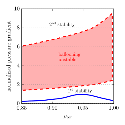
Figure 6: The equilibrium pressure gradient (blue curve, normalized) is prevented from growing steep due to the region of ballooning instability (pink region), calculated by the code BALOO [47].

2.2.3 Transport simulation results

The core scenario resulting from the integrated modeling workflow described above produced a plasma gain $Q_{\text{p}}=11.5$, $P_{\mathrm{fus}}=450\,$MW, $f_{\text{Gr}}=0.88$, $H_{\text{98y2}}$=0.79, and a $P_{\text{SOL}}$ of only 23.5 MW. This value of $P_{\text{SOL}}$ corresponds to a radiated power fraction of 0.82. As discussed in [29], this value is expected to be acceptable for an L-mode-like device. A complete list of MANTA’s parameters is given in Table 1.

The temperature and density profiles are shown in Fig. 7 (a) and (b). The heating sources for electrons and ions are illustrated in Fig. 7 (c). The heat fluxes are well converged from $\rho_{\rm tor}=0.35$ to $\rho_{\rm tor}=0.85$ as seen in Fig. 7 (d). Flux matching between $\rho_{\rm tor}=0.0$ and $\rho_{\rm tor}=0.35$ is known to be difficult, but it has been shown to have a marginal effect on output fusion power due in part to the relatively small plasma volume when compared to the edge [60].

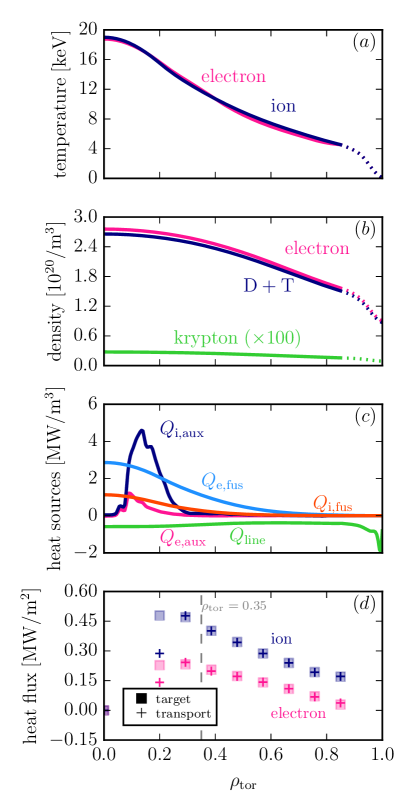
Figure 7: Select TGYRO output profiles versus $\rho_{\text{tor}}$: (a) Electron and ion temperature profiles; (b) Electron, D + T, and krypton (scaled 100$\times$ for visibility) density profiles; (c) Heat deposition profiles for electron auxiliary heating $Q_{\text{e,heat}}$, ion auxiliary heating $Q_{\text{i,heat}}$, line radiation primarily from krypton radiation $Q_{\text{line}}$, electron $\alpha$ heating $Q_{\text{e,fus}}$, and ion $\alpha$ heating $Q_{\text{i,fus}}$; (d) Convergence of electron and ion heat flux profiles.

3 Divertor and Power Handling

For the core scenario to be viable, heat fluxes on the divertor and first wall must be tolerable. These heat fluxes come from two main sources. The first is power transported through the SOL, $P_{\mathrm{SOL}}$, which streams along the open field lines to the divertor targets. The second is power radiated by the plasma via photons, $P_{\text{rad}}$, which more uniformly loads the vacuum vessel. Due to the small plasma-wetted surface area, the divertor targets are at greater risk of failure due to these heat fluxes.

Divertor research has thus focused on methods for mitigating the power fluxes incident on the divertor target plasma facing components (PFCs). This is especially important as parallel heat fluxes in the SOL are expected to increase by an order of magnitude for fusion pilot plants (FPP) compared to current devices [5, 6]. One mitigation method is the use of advanced divertor configurations [61, 62, 63] that feature flux expansion to spread out the heat flux or multiple X-points to distribute the heat flux onto additional targets. However, MANTA’s radiative and NT operation permits a much simpler, conventional divertor to meet the reactor power exhaust challenge.

NT moves the X-points, and hence the entire divertor, to larger major radius. This effect is shown in Fig. 1. The larger circumference increases the area of the divertor targets relative to a PT divertor, spreading out the heat flux. Additionally, ELM-free NT has no lower limit on $P_{\mathrm{SOL}}$, permitting higher levels of impurity seeding than would otherwise be possible. More power may thus be radiated away in the core prior to reaching the SOL, reducing $P_{\mathrm{SOL}}$.

To quantify MANTA’s divertor challenges, the metrics

$$M_{1} =P_{\mathrm{SOL}}B_{T}/{R}$$ (2)

$$M_{2} =(P_{\mathrm{SOL}}B_{T}/R)/n_{\mathrm{sep}}^{2}$$ (3)

are considered for a variety of reactor-class devices. Here, $B_{T}$ is the toroidal magnetic field, $R$ is the major radius, and $n_{\mathrm{sep}}$ is the density at the separatrix. $M_{1}$ is a simple estimate of the relative parallel heat flux density, $q_{||}\propto P_{\mathrm{SOL}}B_{T}/{R}$ (assuming $\lambda_{q}\propto B_{p}$ [64], where $\lambda_{q}$ is the SOL heat flux width, characterized as the e-folding length of $q_{||}$). $M_{2}$ includes the ability of a divertor to dissipate this power flux (since dissipation processes scale according to $\propto n_{\mathrm{sep}}^{2}$, similar to the Lengyel model [65]). The values of these metrics for MANTA, ARC V1 [66], CFETR [67], and EU-DEMO [68] are listed in Table 2. MANTA’s divertor clearly operates in a far less challenging environment than that of other reactor-class tokamaks. This is a direct result of MANTA’s ability to maintain a low $P_{\mathrm{SOL}}$ and high $n_{\mathrm{sep}}$, which is high relative to the core density as a result of smaller edge density gradients in ELM-free NT.

Table 2: Comparison of divertor metrics between MANTA, ARC V1 [66], CFETR [67], and EU-DEMO [68]

Parameter	MANTA	ARC V1	CFETR	EU-DEMO
$P_{\mathrm{fus}}$ (MW)	451	500	558	2000
$R$ (m)	4.55	3.65	7.2	8.8
$B_{T}$ (T)	11.1	11.6	6.5	5.8
$P_{\mathrm{SOL}}$ (MW)	23.5	83	91	150
$n_{\mathrm{sep}}(10^{20}m^{-3})$	0.9	0.61	0.25	0.25
$P_{\mathrm{SOL}}B_{T}/{R}$	57.3	263	82.2	98.9
$(P_{\mathrm{SOL}}B_{T}/R)/n_{\mathrm{sep}}^{2}$	70.7	707	1310	1580

3.1 Optimization of Poloidal Field Coils

Starting from the CHEASE equilibrium, the free-boundary Grad-Shafranov solver FreeGS[69] was used to optimize the poloidal field (PF) coil set and finalize the equilibrium. The goal was to produce the simplest divertor geometry capable of tolerating $P_{\mathrm{SOL}}\approx 25$  MW while maintaining adequate coil lifetimes. This resulted in three pairs of coils with currents similar to other ARC-class designs [5, 29]. Due to the demountability of the toroidal field (TF) coils, the PF coils are placed inside the TFs, reducing their size, current, and cost.

Using the genetic algorithm described in [70], the optimal coil locations were determined by evaluating coil lifetimes (via an approximation of the full neutronics model described in Sec. 5), coil areas, and coil currents for thousands of different possible locations. The coil rotation was also allowed to vary, resulting in the flat face of the coils being presented towards the core as this increased the amount of FLiBe shielding. Additionally, because the solenoid current changes throughout a pulse, this optimization evaluated each coil set at the most positive and most negative solenoid current, resulting in a coil set capable of performing well throughout a pulse. The optimal coil set and resulting equilibrium is presented in Fig. 8 at the time slice of maximum solenoid current. The current, size, locations, and additional details of the PFs are given in Table 5. The engineering considerations of the PFs are detailed in Section 4. The PF lifetimes are given in Section 5.

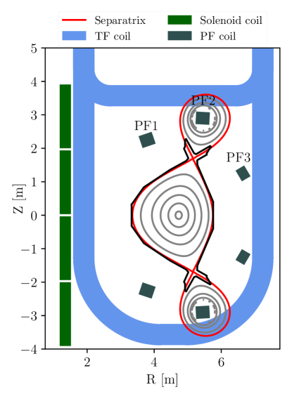
Figure 8: Poloidal cross-section of MANTA showing the full set of REBCO-based superconducting coils and the resulting plasma equilibrium at maximum central solenoid current.

3.2 UEDGE Simulations of Scrape-Off Layer (SOL) Plasma

Using the divertor geometry generated by FreeGS, the heat and particle flux along the open field lines to the divertor target plates were calculated with the 2D edge transport code UEDGE [71]. UEDGE solves the Braginskii fluid equations for magnetized plasmas in the tokamak SOL to determine the steady-state plasma density, temperature, power and particle flows. It also utilises a fluid model to include computation of neutral dynamics and particle sources over the simulation domain. UEDGE has been previously applied to study divertors in high-field reactor-class devices [63, 72] and is here used to refine the point-design and quantitatively assess divertor and power exhaust performance.

The simulation grid was created using the built-in UEDGE mesh generator. The resolution of the grid was increased near the separatrix and near the targets to resolve the steep plasma gradients and neutral recycling physics. At the outer midplane (OMP) separatrix, the grid resolution was chosen to be on the order of the gradient lengths associated with the parallel heat flux. Since MANTA operates in a double-null configuration, only the bottom half of the SOL was simulated to reduce computational cost. A non-orthogonal grid was used to allow fine-tuning of the target geometry relative to that of the field lines as imposed by the FreeGS equilibrium. The field line grazing angle on the divertor targets is ${\sim}3.25\degree$. Smaller angles were prevented by mesh cell distortion.

An input power of $P_{\mathrm{SOL}}=25$ MW was applied at the radially innermost boundary of the UEDGE simulation domain, divided evenly between ions and electrons for simplicity. This is marginally higher than the 23.5 MW obtained from transport simulations in Section 2 due to numerical difficulties related to detachment preventing a smaller $P_{\mathrm{SOL}}$ case from converging. These same numerical difficulties forced a separatrix density $n_{\mathrm{sep}}$ of $0.85\times 10^{20}$ $m^{-3}$, rather than the $0.9\times 10^{20}$ $m^{-3}$ value used in the core modelling. Between the larger tilt angles, higher $P_{\mathrm{SOL}}$, and lower $n_{\mathrm{sep}}$, the results presented here are a conservative estimate for the divertor performance, and the divertor heat flux is likely lower than that calculated here.

Extrinsic impurity seeding [73, 74, 75] in the SOL was required to reduce the power incident on the divertor targets. Neon was selected as the radiator for its low atomic number, ability to radiate effectively at SOL temperatures, and the inertness and recycling benefits of noble gases. Impurity seeding was included in UEDGE via a fixed-fraction impurity model, where the impurity density $n_{\mathrm{imp}}$ was chosen as a fraction of the main ion density, $f_{\mathrm{imp}}=n_{\rm imp}/n$. An additional benefit of not operating in H-mode is the lack of a edge transport barrier; accumulation of impurities in the core is not expected and thus seeding of impurities in the SOL is unlikely to be problematic.[76]

Transport coefficients are chosen to match expected scalings for the heat flux width and in-out power asymmetries. Multi-machine scalings for type-I ELMy H-modes [77] and high-field specific scalings across confinement regimes [78] indicated that for MANTA’s $B_{p}$, $\lambda_{q}$ could be as small as $0.3$ mm. On the other hand, a PT L-mode specific scaling [79] predicted $\lambda_{q}$ of at least a few mm. Recent work on DIII-D and TCV in NT places $\lambda_{q}$ between $\lambda_{q}$ for H-mode and PT L-mode[80, 81]. As a compromise between the different scalings, the transport model was chosen to give $\lambda_{q}=0.9$ mm, as measured using an exponential fit to $q_{||}$ at the divertor throat. In order to reach small enough $\lambda_{q}$ predicted by the $B_{p}$ scaling, the ion and electron heat diffusivity, $\chi_{i,e}$, was reduced to below $10^{-2}$ m²s^-1.

Evidence exists for ballooning-like transport on the LFS [82], implying a larger flow of plasma to the outer than inner divertor. Double-null configurations are known to produce larger in-out asymmetries ($>$80% power exhausted on the LFS) due to the HFS and LFS SOLs being magnetically disconnected [83, 84]. The power split may not be as asymmetric in NT due to the decreased volume on the “bad curvature” side when compared to PT, resulting in reduced interchange-driven turbulence on the LFS [85]. MANTA therefore assumed a 70/30 power split between the outer and inner divertors respectively. This is done by increasing $\chi_{e,i}$ at the outboard side of the simulation grid relative to its value at the inboard side. The particle diffusivity, $D$, was chosen such that density gradient scale length $\lambda_{n}=\frac{n}{\nabla n}\approx 6-10$ mm, as expected at the separatrix in L-mode-like plasmas [86, 87]. Since an H-mode like transport barrier and resulting pedestal is not expected in ELM-free NT operation, flat transport profiles are used in the radial direction.

Though ⁴He is not explicitly modeled in UEDGE, a pumping condition is still applied in the domain to the main ion species to account for ⁴He removal and the impact on divertor neutral gas pressures, plasma flows, etc. Assuming that 2% of the plasma exhausted from the core is ⁴He, and an enrichment of $\sim$0.75 in the divertor (consistent with previous studies[88]), the pumped main ion flux required to be removed in steady-state is found to be $\sim 10^{22}$ particles/s. This condition is applied as a fixed particle flux removed from the simulation domain across the UEDGE private flux region boundary cells in the region identified in Fig. 9 (a), placed close to the outer target where neutral gas densities are highest for efficient pumping. The values for the physics parameters chosen for the UEDGE simulation are tabulated in table 3.

Table 3: Principal control parameters used in UEDGE simulation.

Parameter	Value	Units
$P_{\mathrm{SOL}}$	25	MW
$n_{\mathrm{sep}}$	0.85	$\mathrm{10^{20}m^{-3}}$
$f_{\rm Ne}$	0.315	$\mathrm{\%}$
$\Gamma_{\rm pump}$	5 $\times 10^{21}$	$\mathrm{s^{-1}}$
$\chi_{\rm i/e,out}$	$1.5\times 10^{-2}$	$\mathrm{m^{2}s^{-1}}$
$\chi_{\rm i/e,in}$	$4\times 10^{-3}$	$\mathrm{m^{2}s^{-1}}$
$D$	$2.5\times 10^{-2}$	$\mathrm{m^{2}s^{-1}}$

3.2.1 Edge Modeling Results

The results of the UEDGE simulations are shown in Fig. 9. Plotted in (a) is $T_{e}$ in the lower half of MANTA’s SOL, where the inner leg and more generally the HFS are significantly colder than the outer leg and LFS due to the prescribed 70/30 outer/inner power split. There are no up-down asymmetries present in the simulation as drifts were not included. Fig. 9 (b) shows upstream $n$, $T_{e}$, and $T_{i}$ profiles at the outer midplane.

Figures 10 (a) and (b) illustrate the divertor heat flux and temperature profiles, which ultimately dictate divertor survivability. The inner target is fully detached and the outer target is partially detached. With an impurity fraction of just 0.315%, the more heavily loaded outer target has a peak heat flux of only 2.8 MW/m², well under the usually quoted heat flux limit of 10 MW/m² [89]. However, this target experiences a maximum $T_{e}=6.3$ eV and $T_{i}=6.5$ eV, slightly higher than the desired $5$ eV limit to minimize W sputtering [90]. These maxima occur $15$ mm and $47$ mm from the strike point, much farther into the SOL than the peak of the heat flux profile, ($\sim 2$ mm from the strike point), where the particle flux is much lower and therefore may not present a large concern.

To evaluate the level of W erosion, sputtering dynamics under the present target conditions are analysed for the D, T, He and Ne species. At conditions for $T_{e}<10$ eV, sputtering contribution from D-T ions is negligible[91], such that sputtering is primarily driven by impurities. The impurity ion impact energies (taking $E_{in}=3ZT_{e}+2T_{i}$, where Z is the average charge state[91]) are evaluated and related to the relevant sputtering yield $Y_{W}$ data. At $T_{e}\sim 5$ eV, $E_{in}$ is below the sputtering energy threshold for helium (117 eV)[92], hence no sputtering contribution is anticipated for the He species. Neon sputtering yield is evaluated at $Y_{W}\sim 10^{-4}$ for $E_{in}=40$ eV [93, 94, 94]. Main ion particle fluxes around the target $T_{e}$ peak are at maximum $\Gamma_{D}\sim 1\times 10^{22}$ m^-2s^-1. Combining $Y_{W}$ and $\Gamma_{D}$ with Equation (3) in [94], the W sputtering erosion rate from 0.315% Ne fraction is estimated at 0.0016 mm/year - therefore having no impact on the divertor lifetime.

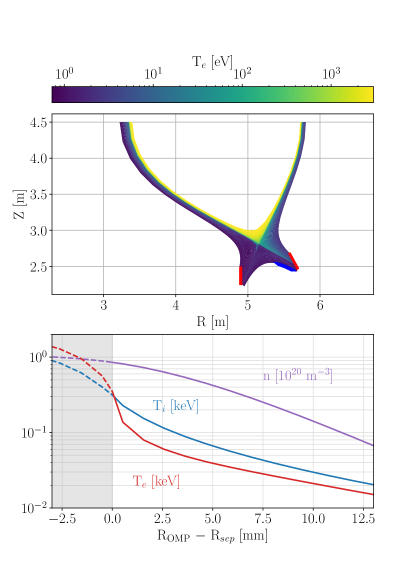
Figure 9: (a) 2D contour of electron temperature ($T_{e}$) for the final UEDGE solution. The outer and inner targets are shown in red and the pumping surface is shown in blue. Note the much larger temperatures in the outer SOL than in the inner SOL. (b) Upstream profiles of $n$ (purple), $T_{i}$ (blue), and $T_{e}$ (red) at the outer midplane (OMP). The gradient scale lengths at the separatrix are smaller for the temperature than the density

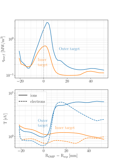
Figure 10: (a) Heat flux density arriving at the inner (orange) and outer (blue) divertor targets. The heat flux density is much larger on the outer target, expected from the in-out power asymmetry modeled. (b) $T_{i}$ (solid line) and $T_{e}$ (dashed line) on inner target (orange) and outer target (blue). Temperatures near the strike point are well below 5 eV on both targets. $T_{e}$ and $T_{i}$ peak above above 5 eV at least $15$ mm from the strike point.

3.3 Divertor and Vacuum Vessel Heat Removal

Active cooling of the first wall components was required, and focus in this study was given to developing a scheme for cooling the divertor targets as they must withstand the highest local heat fluxes. This is achieved via FLiBe channels in direct contact with the backside of the targets, arranged in 18 toroidal segments around the VV. A poloidal cross section of a target is given in Fig. 11.

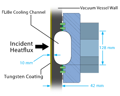
Figure 11: Poloidal cross section of a VV-wall divertor target with a FLiBe cooling channel. The tungsten plasma-facing surface is indicated in gold, the alloy sealing gaskets are highlighted in green, and the external channel block is colored blue.

Ansys Fluent[95] was used to predict the temperature this target design would experience due to the heat flux calculated by UEDGE. The total mass flow rate of the FLiBe was taken to be 20.7 kg/s, resulting in a bulk velocity of 1.5 m/s. In these simulations, the VV wall was considered a single piece of tungsten to avoid simulation artefacts in the thin geometries. This simplified model also neglected toroidal curvature, fasteners, as well as any additional heat removal through the gasket interface. The temperature around the inlet and outlet were not included in the simulation as they were not optimized. The resulting target temperature is shown in Fig. 12, where the maximum temperature is only ${\sim}930\degree C$, well below the recrystalization temperature of tungsten ($1550\degree C$[96]).

A conformal vacuum vessel (VV) design was chosen to maximize the tritium breeding ratio (TBR) and magnet shielding. A gap of 10 $\lambda_{q}$, or about 1 cm between the separatrix and VV was chosen to ensure the vast majority of $P_{\mathrm{SOL}}$ enters the divertor region and does not interact with the VV. Active cooling of the VV was not fully investigated, but one potential solution is a double-walled VV in which FLiBe flows between the two shells and exhausts into blanket tank along with the divertor coolant.

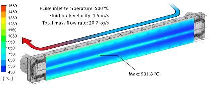
Figure 12: Results of the CFD simulation for the outboard divertor target. Perpendicular inlets and outlets were included to improve fluid fidelity, and the thermal results span between those ports. The bulk temperature increases along the length of the panel. The peak temperature remains far below the Tungsten recrystalization temperature ($1550\degree C$).[96]

4 Magnet Design and Device Maintenance

MANTA’s high magnetic field is produced by 18 non-insulated REBCO HTS toroidal field (TF) coils, a technology pioneered by the SPARC Toroidal Field Model Coil (TFMC) project [97, 98, 99]. The central solenoid (CS) and poloidal field (PF) coils are also made of REBCO tape, though the need for low AC losses and fast response required insulated magnets composed of PIT-VIPER-like cables [100]. All magnets are operated at 20 K with liquid hydrogen (LH2) coolant. Additionally, MANTA was designed around maintaining a reasonable duration for its maintenance cycles, which is primarily a function of the magnet ramp times and cryostat thermal cycling.

4.1 Toroidal Field Coils

The TF magnet design was driven by the need to achieve 11 T on axis while minimizing the required length of REBCO tape, keeping stress within engineering tolerances, and maintaining enough FLiBe between the plasma and the coil for neutron shielding. Additionally, the TFs are designed to be demountable to allow for maintenance and replacement of internal components, namely the vacuum vessel (VV) and PF coils. Several shapes were evaluated for how well they could accommodate all of these requirements, including the traditional “Princeton Dee” [101], a reversed Dee, and “window pane” [102].

The final shape, shown in Fig 13, is a variation of the window pane design. Of the several shapes evaluated with COMSOL [103], this design minimized peak stress while accommodating the joints. At full-field, the maximum von Mises stress is 600 MPa. This is acceptable for the chosen baseplate material, Inconel-718, which has a yield strength above 1000 MPa at cryogenic temperatures [104].

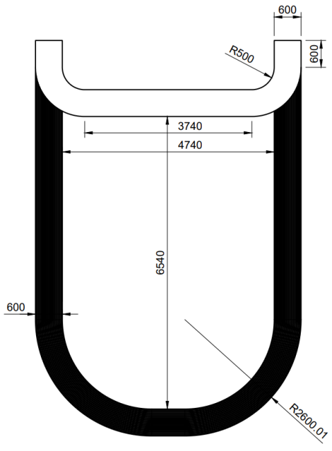
Figure 13: Schematic showing TF 2D planar dimensions in mm. Total TF azimuthal thickness is 544mm. Each of the 18 pancakes is 28mm thick. The magnet casing adds another 40mm to the azimuthal thickness, making the total azimuthal thickness of the TF 544mm.

COMSOL simulations indicated $13.6$ MA-turns were required to produce the necessary 11 T field on axis. To achieve this, each TF is made up of 18 pancakes with 16 turns per pancake, giving an operating current $I_{\rm op}$ of $47.2$ kA. The REBCO tape stack was designed with a height $h$ of $4$ mm and a width $w$ of 21 mm, resulting in an operating current density $J_{\rm op}$ of $570\,\text{A}/\text{mm}^{2}$. This gives a $40\%$ margin below the 25 K and 25 T critical current density of $J_{c}=1000\,\text{A}/\text{mm}^{2}$. This $\rm J_{c}$ is obtained from recent experimental data from commercially available superOx tapes with magnetic fields up to 30 T[105]. The magnetic field in this experiment was aligned perpendicular to the plane of the tapes, a worst case scenario for $J_{c}$.

While a detailed quench resilience analysis is outside the scope of this paper, given the evolving nature of the field, quench resilience needs are anticipated by making room for a $3\times 21$ mm copper cap, a leading approach to improving quench resilience of the magnet [106]. To ensure variations in the radial current between magnets do not cause unacceptable toroidal ripple fields, the approach detailed in [107] is used, where rib thicknesses and nominal joint resistances are designed to be low enough such that the radial current fraction, $I_{r}$/$I_{\rm op}<0.5$%. This is done by setting:

$$d_{\rm rib}\geq\frac{2R_{j}h\cdot\text{max}(l_{\rm up},l_{\rm low})}{\rho_{p}}\left(\frac{I_{\rm op}}{I_{r}}-1\right),$$ (4)

where $d_{\rm rib}$ is the rib thickness, $R_{j}$ is the resistance per joint, $h$ is the height of each tape stack, and $\rho_{p}$ is the baseplate resistivity. Fig. 14 provides a cross-sectional view of the TF showing how key elements fit within the geometrical constraints of the pancake.

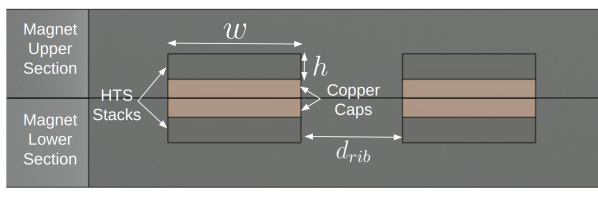
Figure 14: Cross-sectional view of the magnet at the joint, where the upper and lower sections meet.

Table 4: TF Coil Parameters

Symbol	Parameter	Value	Units	Symbol	Parameter	Value	Units
$N_{\rm tf}$	Number of TFs	18	-	$I_{\rm op}$	Operating current	47.2	kA
$N_{\rm pan}$	Pancakes per TF	18	-	$J_{\rm op}$	Operating current density	570	$\text{A/mm}^{2}$
$N_{\rm tpp}$	Turns per pancake	16	-	$J_{\rm crit}$	Critical current density	1000	$\text{A/mm}^{2}$
$L$	Inductance	5.62	H	$R_{\rm rpt}$	Radial resistance per turn	150	n$\Omega$
$W_{\rm TF}$	Stored energy	6.27	GJ	$R_{c}$	Characteristic resistance	40.4	$\mu\Omega$
$d_{\rm rib}$	Rib thickness	0.016	m	$\rho_{p}$	Baseplate resistivity	0.982	$\mu\Omega$-m
$l_{a}$	Azimuthal thickness	0.544	m	$R_{j}$	Resistance per joint	0.5	n$\Omega$
$l_{r}$	Radial thickness	0.6	m	$w$	Width of each REBCO stack	0.021	m
$l_{\rm up}$	Upper mean length	7.455	m	$h$	Height of each REBCO stack	0.004	m
$l_{\rm low}$	Lower mean length	19.2	m	$h_{\rm cu}$	Height of the copper cap	0.003	m

4.2 Maintenance

Maintenance in a reactor-class tokamak is expected to be extremely time-consuming due to the nuclear environment in the vessel, the limitations of remote maintenance, and the time required for the magnets to ramp-up/down and for the cryostat to cool/warm [108]. Past ARC-class concepts have proposed to hasten maintenance cycles by demounting the top of the TF coils and replacing the VV wholesale [19]. This scheme could allow for faster VV replacement than traditional approaches, which instead rely on removing heavy blanket modules through the gaps of the magnet cage [109].

MANTA expands on the demountable magnet philosophy in two ways: 1) replacing the FLiBe tank, PF coils, and VV together (jointly referred to as the “internal assembly”) and 2) oversizing the cryoplant relative to the cooling power requirements of nuclear operations. Removing the internal assembly in one piece eliminates the need to open the FLiBe tank during VV replacement, thereby significantly reducing the dose rate that equipment and workers would be exposed to (see Section 5.3 for more details). This enables safer and quicker FLiBe tank replacement.

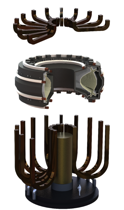
Figure 15: During maintenance, the TFs are demounted, and the VV, FLiBe tank, and PFs are extracted together as a single unit.

The oversized cryoplant is key to reducing the two rate-limiting maintenance steps: TF magnet charging and temperature cycle time. Traditional insulated superconducting magnets can be ramped quickly by driving high voltages, but doing so in non-insulated magnets drives radial currents, which heat the magnet. Current-ramp rates in non-insulated magnets are therefore constrained by the cryogenic cooling capacity, which in practice causes non-insulated coils to take far longer to cycle. For example, KSTAR can fully ramp its insulated TF coils in ${\sim}$30 minutes [110], while the SPARC Toroidal Field Model Coil (TFMC) required ${\sim}$20 hours to charge [97]. Equation 5, derived in A.1, provides the following bound on the maximum magnet ramp-rate:

$$\frac{dI_{\rm op}}{dt}\leq\frac{\sqrt{R_{c}P_{\rm ramp}}}{L},$$ (5)

where $L$ is the magnet inductance, $R_{c}$ is the magnet characteristic resistance, and $P_{\rm ramp}$ is the cooling power available to a single TF to remove heat generated due to magnet ramping. The inverse dependence on inductance exacerbates the current-ramp-rate problem for large non-insulated magnets such as those on MANTA, which have 40x higher inductance than the SPARC TFMC [97]. A simple extrapolation from the SPARC TMFC with constant $R_{c}$ and $P_{\rm ramp}$ would stretch the charging time to over 67 days. $L$ is driven by the on-axis field requirements and system geometry and is thus not significantly adjustable. $R_{c}$ is driven by rib thicknesses which are ultimately limited by the magnet geometry. Thus, the primary adjustable variable to decrease the magnet ramp time is $P_{\rm ramp}$.

To achieve reasonable magnet charging times, $P_{\rm ramp}$ must far exceed the requirement for keeping the magnets at cryogenic temperatures during nuclear operations, $P_{\rm nuc}$. Neutronics calculations (Section 5) indicate that 2.1 kW of heat is deposited in the TFs by neutrons and an additional 0.20 kW in the PFs when MANTA is operating at a typical 450 MW. Owing to the excellent shielding provided by the FLiBe, this is small compared to the 11.5 kW of joint heating. Setting $P_{\rm ramp}=(13.8\text{ kW}/18\text{ TFs})=0.77$ kW/TF would result in a ramp-down time of 42.6 days. Taking into account the equally-time consuming ramp-up time and neglecting any repair time, a single unscheduled maintenance event per year would reduce the plant’s availability by 22.3% [108]. This is clearly unacceptable for a power plant; for comparison, the global nuclear industry averages an Unplanned Capability Loss Factor of 3-6% [111].

MANTA’s cryosystem was therefore designed to provide 200 kW of cooling power during the magnet ramp phase, reducing the magnet cycle time to just 4.6 days. The cost of this oversized cooling power is more than offset by the higher availability factor this implies. Such a large cryoplant is also beneficial for quickening the temperature cycle of the cryostat (i.e. the time to go from cryogenic temperatures to room temperature, and back again). The temperature cycle of the KSTAR cyrostat lasts several weeks[112], and the temperature cycle for ITER will be similar [113]. To emphasize again, weeks-long delays before maintenance can begin will severely affect plant availability.

The energy required to increase the TFs from 20 K to 300 K was estimated by assuming there is approximately 1.1 million kg of Inconel-718 and 0.3 million kg of REBCO. REBCO’s properties were approximated by a 44%/56% mix of copper and Hastelloy. The specific heat of Inconel and Hastelloy were approximated by that of stainless steel, similar to [114]. Numerically integrating over empirical specific heat curves yielded an estimate of 140 GJ of warming/cooling energy required to raise/lower to complete a temperature cycle of the TFs. In order to achieve a week-long warming/cooling cycle time and take advantage of the availability and low-cost of liquid nitrogen (LN2), a two-step temperature ramp process was assumed. When temperatures of are above 77 K, LN2 is used as a precoolant for LH2, increasing the cooling power up to 500 kW. Below 77 K, 200 kW of cooling power is available, the same as during the magnet ramps. While this first step will take 3.0 days, the low specific heat of steel and copper at cyrogenic temperatures enable the second step to be completed in only 0.46 days. This results in a total temperature cycle time slightly less than one week.

A schematic of the entire maintenance cycle is shown in Fig. 16. Cooling channels in the magnets must be designed to handle these non-standard cooling and heating powers over a wide temperature range. While not a trivial problem, these fast magnet and temperature cycle times are essential for a pilot plant (which may face unscheduled maintenance often) and for power plants (which must achieve high availability factors). A traditional ARC-class device with a 42.6 day magnet ramp time and a three-week long temperature ramp time would be offline for at least six months for any maintenance event, but MANTA with “oversized” cooling/heating power can complete both cycles in 16.1 days.

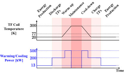
Figure 16: A diagram of the maintenance cycle in terms of temperature of the TFs and cooling/warming power.

4.3 Central Solenoid and Poloidal Field Coils

The mechanical stability of the Central Solenoid (CS) and Poloidal Field coils (PF) was investigated with a 2D-axisymmetric finite element model developed in COMSOL Multiphysics[103]. The CS and PFs are modeled as homogenized multi-turn coils consisting of VIPER cables [100] with four twisted tape stacks. The contribution of the plasma current to the overall magnetic field is approximated by a single-turn elliptical cross section coil with a uniform current profile. The geometry, materials and boundary conditions on this model are detailed in A.2.

To maximize the magnetic flux available to drive the plasma current while respecting engineering stress limits, a maximum operating current density of $J_{\rm op}$ = 80 A/mm² was selected. This choice affords a 25% margin to the VIPER cable critical current at 20 K and 25 T. This current density, together with MANTA’s 3.2 m inner bore diameter, allows the CS to provide 260 Wb of flux with a peak field of 25 T on the CS coils. Using the flux consumption approximations for startup from [115] and the loop voltage calculated from the equilibrium, 260 Wb produced a pulse length of ${\sim}15$ minutes.

The largest stress in the CS occurred at zero solenoid current $I_{\text{CS}}$ due to the TF coil hoop stress, which produced a large unbalanced radial force at the CS-TF boundary. When $I_{\text{CS}}\neq 0$, this force is opposed by the hoop force in the CS. At $I_{\text{CS}}=0$, model predicted a maximum (hoop) stress component of 920 MPa, as shown in Fig. 17. This excludes epoxy as a structural material, but the stress remains below the yield stress of Inconel-718 ($\sim$1000 MPa). While 920 MPa is above the 700 MPa limit at which point $J_{c}$ is diminished[116], the peak field on coil declines simultaneously and the margin between J_op and J_c increases. While the CS is not expected to quench during the current ramp, time-dependent simulation of a realistic geometry is necessary.

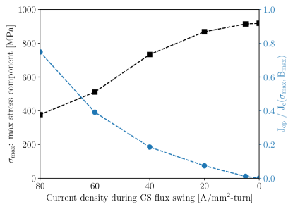
Figure 17: Throughout the current swing of the CS, the maximum stress component remains below the yield stress of Inconel ($\rm{\sim}1000\,MPa$) and the critical current density of SuperOx tapes at 20 K and 25 T under electromagnetic stress loading.

The 8 T peak field on the PF coils permitted a higher $\rm J_{op}=175\,A/mm^{2}$ while retaining more than 30% margin with respect to $\rm J_{c}$[105]. With a larger current density, the coils can be made smaller, reducing their cost and easing the neutron shielding requirements. Details of the PF coils are listed in Table 5. To ensure their ability to generate the desired magnetic geometry is not affected, a PFs were required to be displaced at most 1 cm. This was readily satisfied as the maximum predicted displacement was less than 1.7 mm.

Table 5: Poloidal field coil parameters

Parameter	PF1	PF2	PF3	Units
Max Current$\cdot$turns	7.74	7.51	5.13	[MA$\cdot$turns]
Number of turns	86	84	59	-
Height	0.327	0.29	0.14	m
Width	0.365	0.327	0.215	m
R	3.79	5.45	6.65	m
Z	$\pm$2.25	$\pm$2.9	$\pm$1.25	m
Rotation	108.7	86.8	30.5	degree

5 Nuclear Analysis

MANTA’s blanket system consists of components to extract energy, produce tritium, and shield other systems from the neutrons generated in the core. This section describes the blanket geometry, material selection, blanket power multiplication factor, volumetric heat deposition, magnet lifetimes limited by high energy neutron fluence, and damage to the vacuum vessel. Limits on the tritium breeding ratio derived from a fuel cycle analysis will also be discussed.

The design of the blanket system was driven by four key goals in accordance with the NASEM requirements:

1. Achieve a toroidal field (TF) coil lifetime of at least 1000 megawatt-years and maximize poloidal field (PF) coil lifetimes to increase economic viability

2. Maximize the fraction of energy deposited in the blanket to increase reactor efficiency.

3. Minimize activation of reactor components to reduce health risks and facilitate maintenance;

4. Reach a tritium breeding ratio (TBR) of at least 1.02 (based off modeling discussed in Section 5.4).

5.1 Component Geometry and Materials

A liquid immersion blanket, consisting of molten 2LiF-BeF₂ (FLiBe) flowing down and around the vacuum vessel in a toroidally continuous tank, was selected due to the improved reactor serviceability and enhanced TBR relative to traditional blanket designs that rely on tritium breeding modules inside the vacuum vessel containing significant amounts of non-breeding structural material [117].

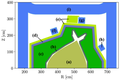
Figure 18: Upper half of a poloidal cross section of the OpenMC model of MANTA. The plasma (a) is surrounded by the vacuum vessel (b). The FLiBe blanket tank (c) is surrounded by layers of WC (d) and B₄C shielding (e). PF coils 1-3 are labeled (f-h) respectively. All components are located within the TF coil cage (i). In order to depict all components in greater detail, the upper portion of the TF joints is cut off.

The Monte Carlo code OpenMC[38] was employed to model the neutron and photon transport throughout the reactor geometry. These simulations were used to guide the choice of material and geometry for the breeding blanket and other shielding components, as well as the location of the magnets. The model employed a fixed neutron source with neutron production profiles based on the transport modeling of MANTA’s fusion core plasma described in Section 2.2. The global variance reduction methodology MAGIC was used to generate weight windows for converging quantities of interest at the magnet locations. The upper half of a poloidal cross section of the model is shown in Fig. 18. Aside from the TF coil (see Fig 14 at a diagram of the TF coil), the geometry is up-down symmetric.

Two 12-cm-thick layers of shielding material surround the blanket tank, with the inner layer made of tungsten carbide (WC) and the outer layer made of boron carbide (B₄C). An additional shield of 42 cm-thick B₄C is located outside these layers above the inner divertor leg to provide further shielding of the TF magnets from neutrons streaming through the divertor. A vanadium-chromium-titanium alloy (V-4Cr-4Ti) was chosen for the vaccum vessel (VV) material, which is predicted to be compatible with the blanket if MoF₆ is dissolved in the FLiBe to generate a self-healing molybdenum barrier at the vessel-blanket interface [118, 119]. Other candidate vessel materials compatible with the FLiBe operating temperature and activation requirements include oxide dispersion strengthened (ODS) ferritic steels and silicon carbide ceramic composites (SiC-SiC). Given MANTA’s modularity, these materials could be explored later in MANTA’s life cycle based on material technological readiness levels [120].

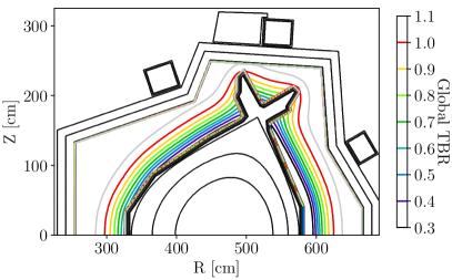
Figure 19: Upper half of a poloidal cross section of MANTA. Overlaid are contours of blanket shapes that achieve a given TBR using the smallest blanket volume possible.

By approximately conforming the blanket tank cross section to contours in local heat deposition and TBR, a design was identified that successfully achieves desired magnet shielding and tritium breeding while making the best use of the space available within the TF coils. Fig. 19 depicts a skeleton of the vessel components within the toroidal field coils overlaid on a contour plot of the global TBR. The contours indicate the smallest blanket shape possible that would achieve the corresponding TBR. This optimization yielded a TBR of 1.15 and a power multiplication factor (as defined in [121] as $M_{f}$) of 1.11, based on heat deposition and lithium reactions occurring in the FLiBe blanket. A summary of the components along with their materials, densities, radial thicknesses, volumes, and volumetric heating is shown in table 6. Heating rates assume energy from secondary electrons is deposited locally. The volumes were calculated stochastically in OpenMC.

Table 6: Neutronics system components along with their materials, densities, radial thicknesses, volumes, and volumetric heating.

Component	Material	Density	Thickness	Volume	Heating
		[g/cm3]	[cm]	[cm3]	[W/cm3/MW${}_{\text{fus}}$]
First wall	Tungsten	19.3	0.3	$(6.8\pm 0.2)\times 10^{4}$	$(4.6\pm 0.3)\times 10^{-2}$
Vacuum vessel	V-4Cr-4Ti	6.05	1.0	$(2.21\pm 0.03)\times 10^{5}$	$(1.75\pm 0.02)\times 10^{-2}$
Cooling channels	FLiBe	1.94	2.0	$(4.55\pm 0.05)\times 10^{5}$	$(1.18\pm 0.02)\times 10^{-2}$
Blanket	FLiBe	1.94	20-100	$(1.367\pm 0.003)\times 10^{7}$	$(2.16\pm 0.01)\times 10^{-3}$
WC shield	WC	15.63	12	$(3.25\pm 0.08)\times 10^{6}$	$(9.6\pm 0.1)\times 10^{-5}$
B4C shield	B4C	2.52	12	$(3.35\pm 0.08)\times 10^{6}$	$(7.0\pm 0.1)\times 10^{-6}$

5.2 Magnet Lifetimes

The blanket and shielding designs were optimized to maximize the TF and PF coil lifetimes, leading to a blanket shape larger than the contours depicted in Fig. 19. Existing studies have predicted the lifetime high energy (above 100 keV) neutron fluence tolerable by REBCO magnets to be $3\times 10^{22}$ neutrons/m² [122, 123]. Because the neutron fluence scales linearly with the fusion power of the core (and to account for potential variable power output from MANTA), magnet lifetimes are reported in units of megawatt-years. Dividing by the device fusion power therefore yields the magnet lifetime at that fusion power. Table 7 summarizes both the lifetime averaged over the cross section as well as the minimum lifetime of each magnet.

The target lifetime of 1000 MW-yr was far surpassed for the TF coils, a major benefit given their high cost (see Section 7). The TF minimum lifetime of ${\sim}3100$ MW-yr corresponds to nearly 7 years of continuous full-power operation at $P_{\text{fus}}=450$ MW. Two of the three PF pairs also surpassed 1000 MW-yr, but PF2 is slightly below due to its proximity to the plasma and thus higher neutron fluence. MANTA’s environmental cycle is therefore set by PF2, which will require replacement every ${\sim}2$ full-power years. Replacement of individual magnets as necessary can be accomplished quickly relative to other reactor designs due to MANTA’s simplified maintenance scheme (Sec. 4.2). In Section 7, these lifetimes are shown to be sufficient for MANTA to meet its economic targets.

Table 7: Mean and minimum lifetimes (in units of MW-yr) for poloidal field (PF) and TF coils based on high energy neutron fluence.

Coil	Mean Lifetime	Min. Lifetime
PF 1	3300 $\pm$ 100	1320 $\pm$ 80
PF 2	3200 $\pm$ 90	890 $\pm$ 40
PF 3	4900 $\pm$ 150	2000 $\pm$ 220
TF	30400 $\pm$ 400	3100 $\pm$ 400

5.3 Vacuum Vessel Activation and Radiation Damage

To estimate the radiological hazard posed by the VV after removal from MANTA, a depletion study was carried out. First, the model was run with the OpenMC transport-coupled operator using tabulated depletion chain data[124] in conjunction with a first-order predictor integrator. The activation analysis used a simplified irradiation schedule, assuming uninterrupted operation at 395MW for 832 days (900MWy). From that point, the integrator was run with no neutron source, allowing materials to decay for 5 years. Photon energy spectra were calculated using material compositions resulting from the activation analysis. The gamma intensity from the vacuum vessel and plasma facing wall are shown in figure 20. V-4Cr-4Ti activation is compared against SS316LN and Inconel 718, two other commonly proposed VV materials. Activation of the V-4Cr-4Ti VV is at least 3 orders of magnitude lower than the other candidate materials at all times, reducing the radiological hazard during maintenance and disposal.

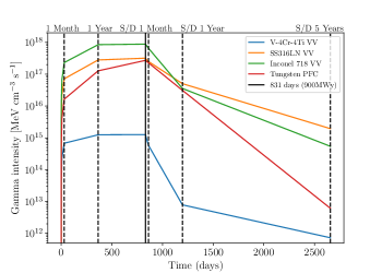
Figure 20: Gamma intensity of the vacuum vessel and plasma facing wall under an irradiation cycle of 900MWy at continuous fusion power of 395MW, followed by 5 years of decay.

The average displacements per atom (DPA) in the vacuum vessel was determined to be 2.24 per 100 MW-yr using the model proposed by Norgett, Robinson, and Torrens [125]. The maximum local DPA rate in the VV was found to be 2.91 per 100 MW-yr. Assuming replacement every 2 full-power years, the resulting average DPA of 19.7 and maximum DPA of 20.5 is expected to be tolerable by the V-4Cr-4Ti[126, 127, 120]. However, this must be verified in situ or with conditions more representative of the first wall.

5.4 Fuel Cycle Analysis

MANTA’s fuel cycle was modeled in the MATLAB Simulink toolbox via an open-source fuel cycle analysis code[128]. This model accounts for (among other factors) tritium startup inventory, fuel burn fraction in the plasma, and tritium losses in the system. Unlike other tokamak systems, a fully functioning tritium fuel cycle has yet to be developed or tested, so the following model employs conservative estimates for model parameters (e.g. tritium losses, system inefficiency, startup inventory, and availability factor).

The fuel system consists of two largely independent cycles: the inner cycle (consisting of the wall, blanket, divertor, etc., responsible for tritium breeding) and the outer cycle (consisting of fuel separation, cleanup, and storage). This design, as well as the estimates for pumping speeds and inherent system losses, were adapted from [129].

Two of the most sensitive parameters of the fuel cycle are the startup and reserve tritium inventories. While the startup inventory can be calculated from other variables, the reserve inventory (i.e. how much extra tritium is stored at the plant) necessitates a balance between radiation safety, cost, and the likelihood of a system failure. Given these constraints, a reserve inventory of 75g was set, resulting in a required startup inventory of 440g was calculated. As tritium fuel systems further mature, these numbers will likely drop, relaxing both economic and safety concerns.

The absolute minimum TBR necessary to sustain plant self-sufficiency with a 440g startup inventory was found to be 1.02. The predicted TBR of 1.15 therefore allows excess tritium production for use to start up future plants. To provide more conservative results, the fuel-cycle simulations assumed a TBR of 1.10. This accounts for unexpected system inefficiencies as well as the future addition of systems that will need to cut through the blanket, thereby reducing its volume and the system’s TBR. This estimate is justified in part by OpenMC simulations that have shown a conservative model of a feedthrough for the RF heating system reduces TBR by about 1%. MANTA’s fuel system will equilibrate within a week (allowing quick return to normal operation following a maintenance cycle) and generate enough tritium to start up another MANTA-class device every six months (see Fig. 21).

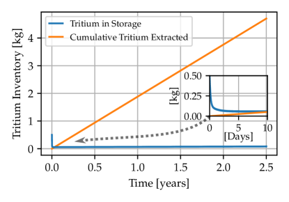
Figure 21: Tritium inventory and production over the plant’s lifetime, assuming a conservative TBR of 1.10. Quickly after beginning operation, the inventory equilibrates to the 75g reserve inventory. Assuming a constant extraction rate, more than 4 kg of tritium are produced in 2.5 years

6 Plant Operation

To ensure that MANTA met the NASEM requirement for minimum electricity production (${\geq 50}$ MWe over $10^{4}$ s) and electricity gain ($Q_{e}\geq 1$), an initial balance of plant and thermal cycle scoping was completed. Multiple thermal cycles were considered, including Brayton, sub-critical Rankine, and super-critical Rankine.

The final design used a steam Rankine cycle fueled by a two-stage molten-salt loop with a thermal storage system to provide constant thermal power to the power cycle for constant electricity production. The plant layout and molten salt storage system are detailed in section 6.2. A steady state net electricity production of at least 90 MWe was achieved at an electrical gain of $Q_{e}=2.4$ for both sub- and super-critical Rankine cycles. The final cycle selection and performance parameters are discussed in Section 6.3.

6.1 Input Constraints and Performance Parameters

Aside from the performance requirements set by the NASEM report, the largest driver of MANTA’s thermal plant design was the input thermal power generated by fusion, $P_{\text{fus}}=450$ MWth, and the additional heat produced by exothermic reactions in the blanket. A finite recirculating power was also required for the auxiliary RF heating ($P_{\text{aux,e}}=57$ MWe) and cryogenics ($P_{\text{cryo,e}}=1$ MWe) subsystems. To generate a steady state power output, the molten-salt storage system must store enough energy during the $15$ minute pulse to provide sufficient power to the turbine during the ${\sim}2$ minute interpulse time. Finally, the maximum operating temperature of the vacuum vessel material, V-4Cr-4Ti, under radiation and thermal load set an upper limit of 600°C on the temperature of the hot (FLiBe) leg of the thermal cycle [120].

The total net electrical power, $P_{\text{e,net}}$, was calculated for a Brayton, sub-critical Rankine, and super-critical Rankine power cycle from

$$P_{\text{e,net}}=P_{\text{turb,e}}-P_{\text{systems,e}},$$ (6)

where $P_{\text{turb,e}}$ is the electrical power generated by the power cycle turbine and $P_{\text{systems,e}}=P_{\text{aux,e}}+P_{\text{cryo,e}}+P_{\rm pumps,e}$ is the electrical power to run the subsystems, namely the auxiliary heating, cryo, and pumps/compressors. The turbine mechanical-electrical power conversion efficiency was assumed to be 1, and the pumps’ electrical-mechanical power conversion efficiency was assumed to 0.75. The electricity gain factor $Q_{e}$ is defined such that $Q_{e}>1$ corresponds to net electricity gain, matching the definition in the NASEM report[1].

$$Q_{e}=P_{\rm turb,e}/P_{\rm systems,e}.$$ (7)

A thermodynamic analysis of the overall MANTA plant design was completed to calculate these quantities.

6.2 Plant Layout and Molten Salt Storage System

MANTA’s thermal plant consists of a primary FLiBe loop in which heat is deposited due to fusion, a secondary molten salt loop to isolate the power cycle working fluid from contamination, and a power cycle that generates electricity via a turbine. The thermal storage system was incorporated into the secondary loop to ensure constant thermal power to the power cycle both during a discharge (${\sim}$15 minutes long) and between pulses (${\sim}$2 minutes long).

A constant thermal power has the additional benefits of keeping the turbine at its maximally efficient, rated power output and keeping the pressures and temperatures in the system close to steady-state. The secondary loop and the storage system employ a molten salt mixture of 60% NaNO₃/40% KNO₃, which is a typically used for thermal storage in solar energy plants. This salt was selected here for its boiling and recrystallization points being above the hot-leg temperature of the primary-secondary loop molten salt heat exchanger and below the cold-leg temperature of the secondary-power cycle heat exchanger, respectively [130].

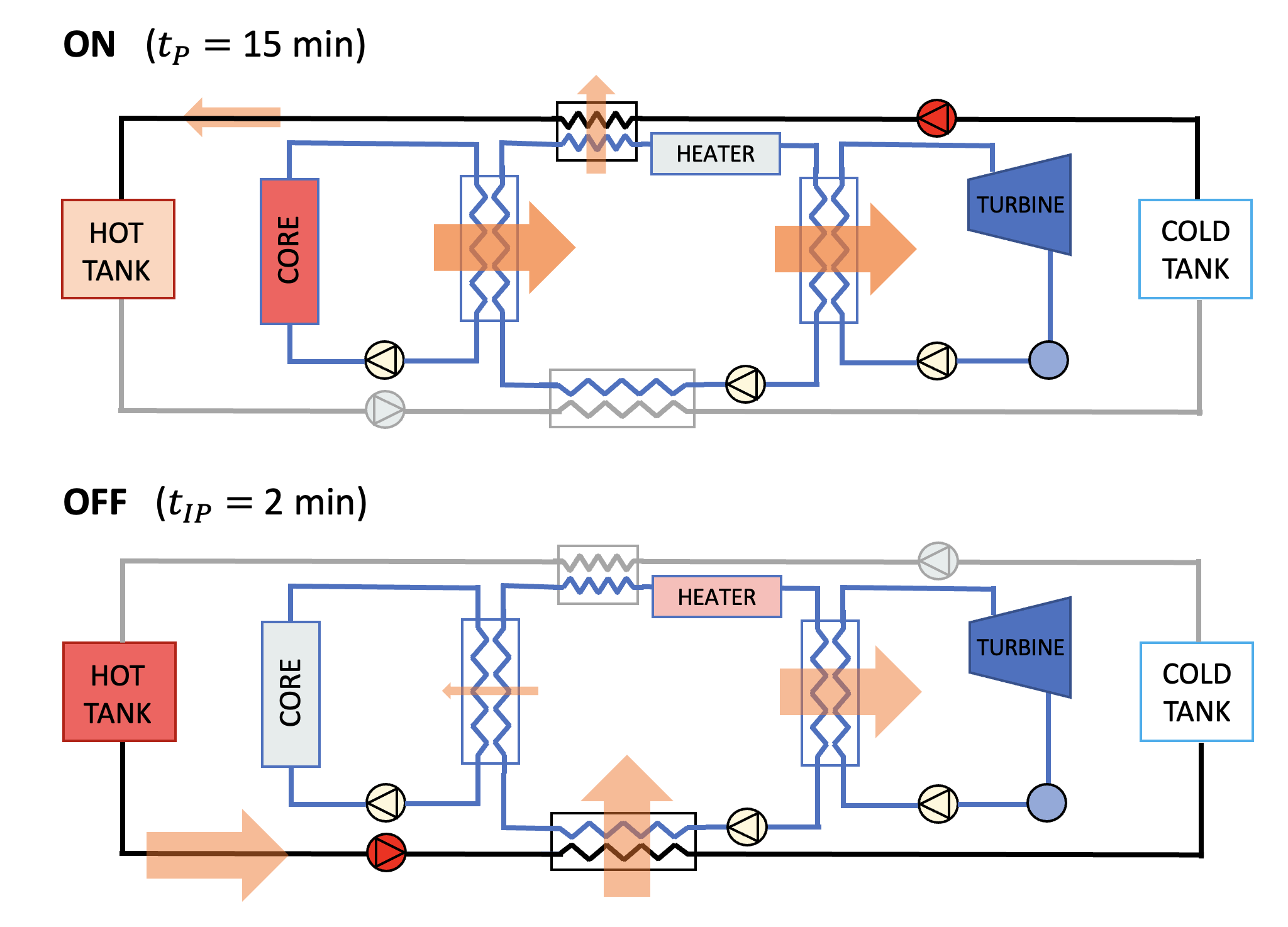
Figure 22: Molten salt loops and power cycle diagram for pulse and interpulse operation. Cycles are connected through heat exchangers between them and to the surrounding storage system. Circumscribed triangles represent pumps: yellow pumps are continuously run, and red/gray pumps are on/off depending on the phase of operation.

A diagram of the complete thermal plant, including the storage system is shown in Fig. 22. The flow of power is highlighted with orange arrows. During a discharge (upper plot), thermal power is captured or generated by the primary cycle and transferred into the secondary cycle. A fraction of this power is tapped from the secondary salt loop and stored in the hot tank via exchange of heat with the cold tank, reducing the thermal power to the power cycle. Between pulses (lower plot), heat is taken from the hot tank to maintain a constant thermal power to the power cycle. In order to maintain the molten salts at constant temperatures between pulses, a small fraction of power is transferred to the FLiBe cycle to balance thermal losses, and a heater is run with some of the power allocated to the auxiliary plasma heating systems, which is not needed during interpulse operation.

To calculate the pulse-averaged thermal power sent to the power cycle, the flow of heat through the various sub-cycles was considered. The gross thermal power from the blanket, including the multiplication factor $M_{f}$ calculated by the OpenMC neutronics simulations is

$$P_{\rm th,gross}=\left[\frac{E_{\alpha}}{E_{DT}}+M_{f}\frac{E_{n}}{E_{DT}}\right]P_{\text{fus}}+P_{\text{aux}},$$ (8)

where $E_{\alpha}=3.5$ MeV, $E_{n}=14.1$ MeV, and $E_{DT}=17.6$ MeV are the energies of fusion-born $\alpha$-particles, fusion-born neutrons, and total released by D-T fusion. $P_{\text{aux}}=40$ MW is the RF power after tetrode electricity-to-RF efficiency. The pulse-averaged thermal power is then

where the heat exchanger efficiencies $\eta_{HX}$ were assumed to be 0.95. The first term represents the thermal power without the storage system contribution, which passes through the primary-secondary loop and secondary-power cycle heat exchangers. The second term is the power tapped stored in the thermal storage system during pulses. The two additional passes through heat exchangers when the core is off result in a temperature drop, which is recovered with the heater.

6.3 Power cycle choice

Three thermal cycles were considered for MANTA: Brayton, sub-critical Rankine, and super-critical Rankine. Brayton cycles typically operate using air or helium as a working fluid, with helium being preferred for its high heat capacity and chemical inertness [131, 132]. Although Brayton cycles are currently used in natural gas power plants and have been proposed for use in high temperature gas cooled nuclear power plants, their effectiveness relies on achieving a high temperature differential across the cycle. Modern Rankine cycles are often supercritical and operate at higher inlet temperatures and pressures to increase efficiency over sub-critical cycles [133]. There are also advantages to using a single-phase, super-critical working fluid, including decreased heat exchanger complexity and reduced degradation of critical turbine components due to water vapor.

A thermodynamic analysis of basic Brayton and Rankine cycles was performed to evaluate performance. The Brayton cycle is closed, has one turbine stage, and uses regeneration to capture heat leaving the turbine, with 80% efficacy [134]. The base pressure is 10 bar, which is relatively high but typical of helium Brayton cycles [132]. At the MANTA design point, the optimized compression ratio was 2.0. The sub- and super-critical Rankine cycles use two turbine stages and include regeneration via an open feedwater heater, which taps some fraction of the heated working fluid from the high-pressure turbine outlet and mixes it with the outlet of the first pump coming after the condenser. The thermodynamic states and regeneration fraction are optimized for maximum thermal efficiency. The maximum pressure is set to 150 and 300 bar for the sub- and super-critical cycles, respectively. The maximum temperature for all cycles is set to 560°C, which considers a 20°C temperature drop across the FLiBe to solar salt and the solar salt to power cycle heat exchangers. This is a conservative temperature drop given the low technological readiness level of molten salt heat exchangers, and is expected to be reduced as these components are further developed. All thermodynamic state analysis and optimization was performed in Python using the pyXSteam[135] and PYroMat[136] libraries. The details of the power cycle models, including thermodynamic properties at the final design point are provided in B.

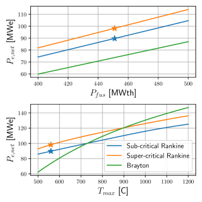
Figure 23: Upper: $P_{\text{e,net}}$ for 3 different power cycles over a range of $P_{\text{fus}}$ at fixed $T_{\text{max}}$=560 °C. Lower: $P_{\text{e,net}}$ for 3 different power cycles over a range of $T_{\text{max}}$ at fixed $P_{\text{fus}}$= 450 MWth. The starred points indicate the final design points for the selected power cycles.

Fig. 23 shows $P_{\text{e,net}}$ for each of the cycles over scans of $P_{\text{fus}}$ (upper plot) and the power cycle maximum temperature, $T_{\text{max}}$ (lower plot). At each value of $T_{\text{max}}$, the Rankine cycle regeneration parameters and Brayton cycle compression ratio are re-optimized for consistency. The $T_{\text{max}}$ scan shows that at the operating $T_{\text{max}}$ of the power loop, both Rankine cycles outperform the Brayton cycle, though Brayton cycles can provide a higher power out at higher temperatures. The $P_{\text{fus}}$ scan at fixed $T_{\text{max}}=560$°C shows both Rankine cycles outperforming a Brayton cycle and that for a wide range of fusion powers around the 450 MWth design point, $P_{\text{e,net}}$ scales nearly linearly with $P_{\text{fus}}$. These scans resulted in the choice of a Rankine cycle for MANTA.

And the large gains in $P_{\text{e,net}}$ at higher $T_{\text{max}}$ demonstrate the benefits of a VV capable of withstanding such temperatures. Alternative VV materials such as oxide dispersion strengthened (ODS) ferritic steels or silicon carbide ceramic composites (SiC-SiC) could be explored later in MANTA’s life to increase electricity production as the technological readiness levels of these materials increase.

Important performance parameters for each cycle are reported in Table 8. The thermal efficiency is calculated for each cycle as the net thermal power out divided by the thermal power in

$$\eta_{th}=(P_{\rm turb,th}-P_{\rm pump/comp,th})/\langle P_{th}\rangle_{\rm pulse}.$$

This definition does not reflect the benefit of coupling the mechanical shaft of the turbine and the compressor in the Brayton cycle, as compared with running electric pumps with a certain efficiency in the Rankine cycles, but this is considered when calculating $P_{\text{e,net}}$. The super-critical Rankine cycle has the best performance, with the highest $\eta_{th}$, $P_{\text{e,net}}$, and $Q_{e}$. The Brayton cycle has a higher $P_{\rm systems,e}$ than either Rankine cycle due to the increased power cost of the gas compressor compared to the water pumps. Notably, all of the considered cycles exceed the NASEM report requirements while conforming to the constraints imposed by MANTA’s various subsystems. Given their superior performance, both Rankine cycles are found to be suitable for MANTA’s electricity generation. The sub-critical cycle was ultimately chosen for the possibility of brownfield siting, which is further discussed in Sec. 7.

	Sub-critical Rankine	Super-critical Rankine	Brayton	Units
$\eta_{th}$	0.36	0.39	0.33	-
$P_{\text{systems,e}}$	63	69	257	MWe
$P_{e}$	90	98	74	MWe
$Q_{e}$	2.4	2.4	1.28	MW${}_{\text{th}}$

Table 8: Performance parameters at the operating point for sub-critical Rankine, supercritical Rankine and Brayton cycles.

7 Economic Analysis

The NASEM report states that a viable pilot plant must achieve an overnight cost of less than US$5 billion, writing “If the private sector, even with government backing …, will not accept a total price past US$5 billion to US$6 billion for generating technology already demonstrated at scale, then it will certainly not accept this for the pilot plant.”[1]. To ensure that MANTA met this requirement, a techno-economic analysis was performed. Critically, a pilot plant must also provide confidence that an $N^{\mathrm{th}}$-of-a-Kind, commercial power plant of a similar design has a path to profitability. With this goal in mind, the levelized cost of electricity (LCOE) for MANTA and a scaled-up power plant version was calculated, accounting for costs across the project lifetime as well as revenue streams.

7.1 Overnight Cost Assessment

Leveraging a bottom-up techno-economic model, an overnight cost of US$3.4B was calculated, more than meeting the NASEM report requirement. As will be detailed below, this value represents the sum of tokamak costs (Table 12), other direct costs (physical infrastructure, Table 13), and indirect costs (service costs, Table 14). A contingency of 10% was added to the total budget, reflecting standard industry practice of building in cost “head room” to increase confidence in a large-scale capital budget[137]. The US$3.4B overnight cost translates to a unit cost of $\simeq$US$38 million / MWe. While MANTA was not designed as a commercial power plant, this is within a factor of two of the Dominion Energy Coastal Virginia Offshore Wind 12 MWe (pilot) plant project built in 2020 [138, 1].

The tokamak itself was predicted to cost US$3.1B, ${\sim}89\%$ of the total overnight cost. The largest cost driver is the toroidal field (TF) coils at US$1.5B, as illustrated by Fig. 24. To cost the tokamak, subsystems were broken into their constituent components wherever possible. Using simplified geometric models of each component, the component mass was then estimated. Total material costs were calculated according to Table 15. To best ensure that the overnight cost stayed within NASEM limits, a conservative model was applied for converting material cost to fabricated component cost. Labor costs (L) were estimated as proportional to the material costs (M), with a fabrication factor of 3x for traditional components and 5x for superconducting magnets:

$$M+L=\text{fabrication factor}*M$$ (10)

This approach is similar to the cost per tonne scaling laws used in [117] and [139]. However, it allowed the impact of materials selection, and their dramatic range in costs, to be explored. Further assessing the techniques necessary for manufacturing each component and using these to refine the labor cost estimates would be a valuable area of future research. The turbine plant cost was estimated from [140], and remaining direct and indirect costs were taken from the ARPA-E report on fusion power plant costs [138].

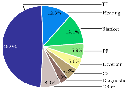
Figure 24: Break down of the major systems contributing to the cost of the tokamak. The tokamak makes up 89% of MANTA’s total cost.

To gain confidence in this costing estimation, a sensitivity study scanning $\pm 50\%$ was performed on the four key cost drivers with most uncertainty: the fabrication factor for traditional components, the fabrication factor for superconducting components, the cost of REBCO, and the cost of FLiBe, the results of which are seen in Figure 25. Throughout this range of values, the overnight cost remained less than the US$5B, increasing the confidence that MANTA meets this requirement.

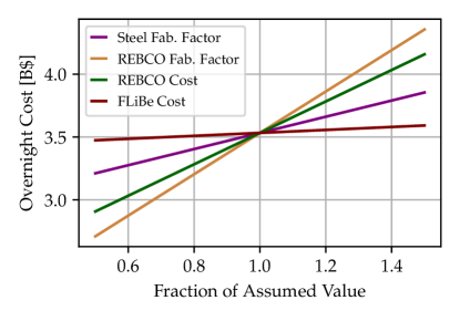
Figure 25: Sensitivity analysis ($\pm 50\%$) of key values assumed in techno-economic modeling. Within this range of values, costs remain under the targeted maximum of US$5B.

It is assumed for this analysis that MANTA is built at a “brownfield” land site (that of an unused fossil fuel plant). This option saves on costs related to the sub-critical Rankine cycle, the electrical plant, and around half of the building construction costs. While legacy plant decommissioning is an additional cost, approximately US$120k/MWe for a coal plant [141], brownfielding saves an estimated US$400 M, or around 5% of the total overnight cost vs a “greenfield” (empty land) site, although this could be a more generalizeable use case.

It is also important to recognize the non-monetizable benefit to brownfielding in the energy justice implications of retaining jobs within communities dependent on fossil fuel plants and putting often marginalized communities at the forefront of cutting edge scientific development. Furthermore, the relatively small contribution to the capital and operations budget of construction and personnel (see Tables 14 and 16 in the Appendix) and extra room in the overall budget indicate that the jobs created to build and run a MANTA-class reactor could provide good pay and benefits (e.g. “Good paying, union jobs”[142] meeting prevailing-wage rates). This is a further component of a just transition to a clean energy economy[143] and one with positive implications in both finance (maintaining eligibility for electricity production tax credits[144]) and policy (maintaining public support for fusion energy[145]).

7.2 Beyond NASEM: MANTA Provides Operational Certainty

While MANTA was not designed to be or directly extrapolate to a commercial powerplant, the design and techno-economic model can help further identify a path to commercially viable fusion energy. Beyond fulfilling the NASEM requirements, this involved an accounting of MANTA’s lifetime costs and revenue streams. The scalings of these factors are succinctly captured by MANTA’s levelized cost of electricity (LCOE), the minimum wholesale price of electricity at which the project becomes profitable:

$$LCOE=\frac{\sum_{t}\frac{C_{t}}{(1+d)^{t}}}{\sum_{t}\frac{P_{e,net}}{(1+d)^{t}}},$$

where $C_{t}$ are the costs at a specific point in time, $P_{e,net}$ is the net electricity generated at that time, and $d$ is the discounting factor (an industry standard 7% [146], necessary to capture the opportunity cost of an investment). The costs included are: financing, personnel, yearly capital degradation, magnet and vacuum vessel replacement, and fueling/selling tritium. See Table 16 for further details, and Section 6 for the derivation of $P_{e,net}$. A conservative “learning” function of

$$L=0.6+0.4\times^{\left[n^{th}~{}unit/5\right]}$$ (11)

is assumed, where $n$ is the total number of a given component produced. This slightly reduces the cost of component fabrication over time[147]. No tax credits or any effective corporate tax rate (even when likely applicable, see Table 16) are assumed as these important factors are too geographically and legislatively dependent. A 3% inflation rate is assumed.

The gross revenue for an 8.5 year project, including selling both tritium and electricity, is estimated to be US$205M, and a gross loss of US$512M (both values include inflation and discounting factors), giving an overall cost of ${\sim}$US$3.7B. This remains under the upper limit of the overnight cost, although without profitability. The cumulative inflow and outflow over time is shown in Fig 26. During periods of magnet replacement the electricity production drops to zero (following Fig. 16).

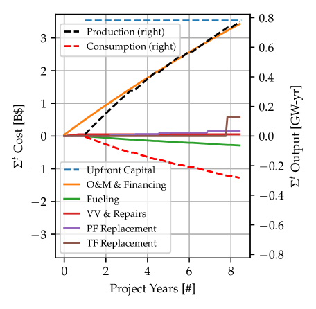
Figure 26: Cumulative cost and electricity inflow/outflows over time for an 8.5 year project, assuming a 1 year construction period. Upfront capital cost shown for reference. Notice the large cost jump at the 1^st TF replacement timepoint and the zero electricity production during magnet replacement (e.g. year #3). See table 16 for further details. Tritium sales represented as a negative cost

The LCOE framework gives a simple intuition as to how model parameters affect the overall economic viability, although without self-consistent physics models. For instance, Fig. 26 shows the sale of tritium and replacement of the TF to be key revenue/cost drivers. Scanning over the market price of tritium and the REBCO fabrication labor multiplier cost (similar to Fig 25) show that a 75% decrease in the former (e.g. due to MANTA’s predicted 1.8kg/yr net tritium production saturating the current 2.7kg/yr global tritium production market[148]), could be balanced by a 30% decrease in the latter by improvements in engineering efficiency. Both of these changes generated a factor of $\times$1.6 change in LCOE.

Finally, the techno-economic model indicated areas of improvement necessary to move from a First-of-a-Kind to a commercially viable $N^{\mathrm{th}}$-of-a-Kind device. The LCOE model was used to investigate a hypothetical device scaled up in power based off of MANTA. Scaling to a 550 MW core (just within the bounds of the POPCON and below the Greenwald limit, see Fig. 3) and a 30 year project gives an LCOE of US$396/MW-hr, assuming current tritium prices. This is significantly too high to be economically competitive, higher even than existing yet novel carbon-neutral technologies, such as offshore wind ($136.5/MW-hr estimated for projects entering into service in 2027[149]).

However, the model suggests a direction for a design point of a future MANTA-based reactor which would move closer to profitability: higher power and longer magnet lifetimes . If the TF & PF lifetimes were extended to exceed the lifetime of the 550 MW project, the LCOE drops by 56%. Similarly, increasing the power cycle efficiency by running the working fluid at 900C (with a vacuum vessel that could handle such a temperature, such as SiC/SiC[120]) decreases the LCOE an additional 10%, making this hypothetical plant comparable to offshore wind’s price point. Thirdly, the POPCON model outlined in Section 2 suggests accessing a higher $P_{\text{fus}}$ regime should be possible without a significant increase in $P_{\text{SOL}}$ or auxiliary heating power (and accompanying RF heating cost), with a similarly dramatic improvement in LCOE (as $P_{\text{fus}}$ approaches e.g. $\sim 1~{}\mathrm{GW}$).

While such operating points have not been self-consistently modeled, it is encouraging that the most detailed economic costing model for a fusion reactor published to date predicted an LCOE even remotely close to profitability. Furthermore, the fact that this is achieved based off extrapolation from a device not optimized for commercial power production and that a path appears to exist towards commercial viability of the high-field NT tokamak concept is highly promising.

8 Conclusion

By leveraging negative triangularity and radiative, ELM-free operation to take a “power-handling first” approach, MANTA (Modular Adjustable Negative Triangularity ARC-class) scales the tokamak concept to a fusion pilot plant (FPP) while maintaining readily survivable heat fluxes on the divertor targets. An extensive integrated modeling workflow confirmed MANTA satisfies the requirements of an FPP for demonstration of the path to commercial viability of nuclear fusion, as detailed in the NASEM report[1]. These criteria are summarized in Table 9, where MANTA is seen to surpass all metrics. Additionally, MANTA’s environmental cycles last ${\sim}$2 full-power-years, making the requirement of operation through several environmental cycles possible in a reasonable amount of time and before the lifetime of the TF coils is reached.

Table 9: Comparison of NASEM criteria and those achieved by MANTA

Parameter	NASEM Requirement	MANTA
$Q_{E}$	1	2.4
$P_{e,net}$ [MWe]	50	90
$TBR$	0.9	1.15
Overnight cost (USD)	$5 Billion	$3.4 Billion

Beyond these criteria, MANTA is designed around its role as a pilot plant, where modifications to both the device itself and the operating point are expected. MANTA’s use of demountable TF coils, a liquid immersion FLiBe blanket, and an oversized cryosystem permit relatively rapid replacement of reactor components, ideal for the prototyping of fusion technology. MANTA’s fusion power can also be adjusted while maintaining constant $P_{\text{SOL}}$ through control of the density, allowing for a flexible operating point. Together, these two features significantly enhance MANTA’s effectiveness as an FPP.

The most essential area of future work will be continuing NT studies on existing devices. Compared to positive triangularity, negative triangularity is far less understood. While MANTA’s success in meeting the NASEM targets together with previous work[15, 16, 17, 18] show the plausibility of NT pilot/power plants, further experimental data, especially with regards to radiative ELM-free plasmas, is required to provide greater confidence that NT can scale to a reactor-class tokamak.

9 Contributions

G.R. led the writing of this work; D.A., S.B., A.R.D., A.D.M., M.C.C., R.C., L.C., J.J., J.v.d.L, M.A.M., A.S., M.T., A.V., A.M.W., and H.S.W. contributed to the writing of this work; G.R and A.S. oversaw project management; J.W. designed the SOLIDWORKS CAD models of MANTA; 0D core solution found by A.S. with contributions from S.B., L.C., R.D., J.D.J, P.L., J.v.d.L, and M.P; CHEASE equilibria generated by R.D., J.v.d.L., and H.S.W.; Initial RF solution identified by J.D.J and S.J.F and finalized by J.v.d.L. and S.J.F.; Initial transport scoping completed by S.B., L.C., and M.P.; Final transport solution scoped and calculated by H.S.W. with contributions by A.S.; L.C., J.D.J., and M.A.M worked on core-edge integration; G.R. generated the FreeGS equilibrium and initial PF coil design; N.d.B optimized the PF coils; D.A. and M.A.M. developed the UEDGE solution with contributions from H.C.; Divertor target FLiBe cooling modeled by J.W. with contributions from C.C.; A.D.M. and A.M.W. developed the maintenance scheme and TF coils; A.R.D and H.S.W modeled the electromechanical properties of the CS and PF coils; J.J. and M.T. analyzed magnet lifetimes with contributions from J.L.B.; J.J. investigated vacuum vessel activation with contributions from J.L.B.; Tritium fuel cycle calculations completed by N.D.; Pulse duration calculated by G.R. with contributions from A.R.D. and S.M.; Balance of plant analyzed by M.C.C. and A.V. with contributions from S.M.; A.S. calculated the overnight capital cost; LCOE analysis completed by R.C.; S.J.F, C.J.H, N.R.M, and P.R.F mentored the core group; A.O.N and M.W mentored the divertor/power-handling group; T.M. mentored the magnets group; S.F., E.P., and S.S. mentored the neutronics group; R.B. mentored the economics and balance of plant groups; and C.P.S. and D.G.W. oversaw this work.

10 Acknowledgements

The authors are grateful to all other course members of MIT 22.63/CU-APPH 9143 and for the expert advice of Matt Reinke, Nicolo Riva, Sergey Kuznetsov, Tony Qian, Adam Kuang, Jacob Schwarz, Rui Vieira, Charles Forsberg, Ted Golfinopoulos, as well as to Sean Ballinger for use of his UEDGE post-processing tools. This work was supported in part by US DOE grants DE-FC02-04ER54698, DE-FG02-86ER53222, DE-FG02-91ER54109, DE-SC0007880, DE-SC0014264, DE-SC0018623, DE-SC0020415, DE-SC0021311, DE-SC0021325, DE-SC0021622, DE-SC0021629, DE-SC0021657, DE-SC0022012, DE-SC0022270, DE-SC0022272, and DE-SC0023289, the Ida M. Green fellowship, NSF GRFP grant 2141064, “la Caixa” Foundation fellowship LCF/BQ/AA20/11820045, Mauricio and Carlota Botton Foundation fellowship, Commonwealth Fusion Systems, and Eni. Disclaimer: This report was prepared as an account of work in part sponsored by an agency of the United States Government. Neither the United States Government nor any agency thereof, nor any of their employees, makes any warranty, express or implied, or assumes any legal liability or responsibility for the accuracy, completeness, or usefulness of any information, apparatus, product, or process disclosed, or represents that its use would not infringe privately owned rights. Reference herein to any specific commercial product, process, or service by trade name, trademark, manufacturer, or otherwise does not necessarily constitute or imply its endorsement, recommendation, or favoring by the United States Government or any agency thereof. The views and opinions of authors expressed herein do not necessarily state or reflect those of the United States Government or any agency thereof.

11 References

Appendix A Magnet Design and Device Maintenance

A.1 Derivation of Equation 5

Beginning with Eq. 6 from [150]:

$$L\frac{dI_{\rm op}}{dt}+V_{c}\left(\frac{I_{\rm op}}{I_{c}}\right)^{n}=R_{c}(I_{\rm ps}-I_{\rm op})$$ (12)

where $L$ is the coil inductance, $I_{\rm op}$ is the current driven through the superconductor, $I_{\rm ps}$ is the current input through the powersupply, $I_{c}$ is the critical current, $V_{c}$ is the voltage criterion for $I_{c}$, $n$ is the number of turns in the coil, and $R_{c}$ is the characteristic resistance of the radial pathway. For a magnet with many turns and operating with a reasonable margin away from the critical current, $(\frac{I_{\rm op}}{I_{c}})^{n}\approx 0$, so the second term on the left hand side can be neglected, giving:

$$L\frac{dI_{\rm op}}{dt}=R_{c}(I_{\rm ps}-I_{\rm op})$$ (13)

From Ohm’s law, the following inequalities must be satisfied to avoid heating the magnet:

$$R_{c}(I_{\rm ps}-I_{\rm op})^{2}\leq P_{\rm cool}$$ (14)

$$I_{\rm ps}-I_{\rm op}\leq\sqrt{\frac{P_{\rm cool}}{R_{c}}}$$ (15)

where $P_{\rm cool}$ is the available cooling power. Plugging inequality 15 into equation 13 gives:

$$\frac{dI_{\rm op}}{dt}\leq\frac{\sqrt{R_{c}P_{\rm cool}}}{L}$$ (16)

A.2 Finite element model of the Central Solenoid and Poloidal Field Coils.

A.2.1 Geometry of the CS/PF model

The physical dimensions and currents of the six poloidal field coils were chosen to produce a suitable magnetic equilibrium. The dimensions of the central solenoid are a trade off between the space available to the solenoid (3.2 m diameter) and the maximum achievable field within structural and electromagnetic limits, as explained in 4. These design parameters resulted in 0.6 m wide by 7.76 m tall CS with 3296 turns.

Both sets of coils are modeled as COMSOL homogenized multi-turn coils. The number of turns is determined by assuming a rectangular arrangement of turns, which have a square area of 1406 mm², accounting for the structural steel jacket supporting the VIPER cable. The VIPER cable is illustrated in Fig 27 and comprises four square twisted REBCO tape stacks (16 mm²) embedded in a copper matrix. The copper enables current sharing between the stacks and thermal stability by exchanging heat with the central coolant duct[100]. The current carrying cross-section of a turn is the area of the VIPER cable, or 603 mm². The choice of current density per turn in the CS and PF coils is explained in section 4.

The COMSOL calculations also include the effect of a 10 MA plasma current, modeled as an elliptical conductor (1.2 x 1.6 m) with uniform current density.

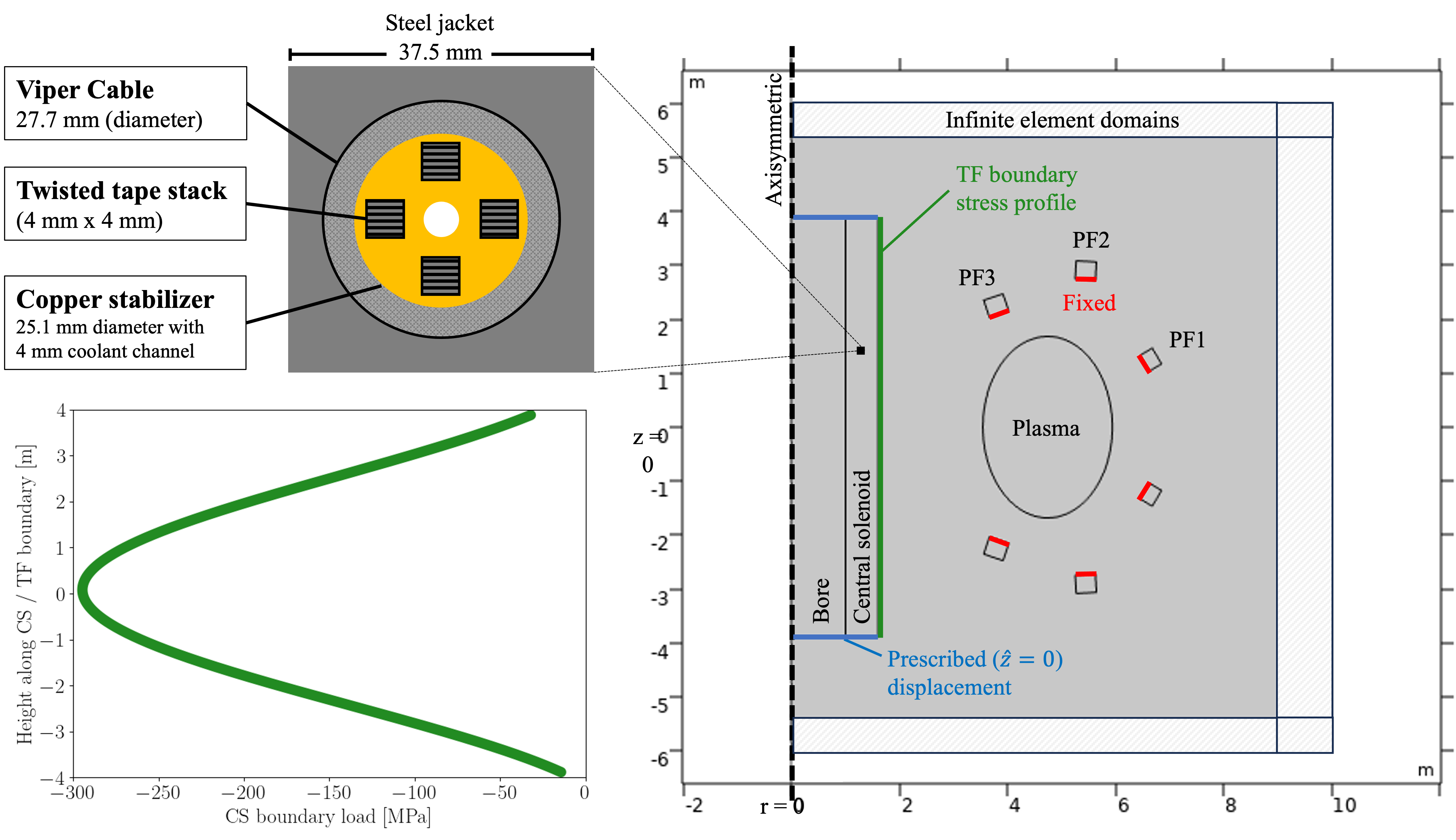
Figure 27: The dimensions and boundary conditions of the Central Solenoid (CS) and Poloidal Field (PF) Coils were set up to produce a full-account of Lorentz stresses and strain, including the effect of a 10 MA plasma and the boundary load on the outer edge of the CS resulting from the hoop stress in the toroidal field (TF) coils.

A.2.2 Materials and boundary conditions

The coils are modeled as a mixed material with 8.5% Cu and 91.5% steel accounting for the fraction of copper in the VIPER cable, and assuming all other parts are made of steel. The bore of the CS is filled with structural steal as a simplest-possible solution to counter the hoop stresses from the TF and CS. A more comprehensive modeling of the CS should nevertheless consider the potential large AC losses incurred by this choice.

The boundary conditions of the model are represented on Fig. 27. Most importantly, the model is axisymmetric about the center of the CS, and the outer boundaries of the air volume surrounding the CS and PF are infinite element domains that extrapolate magnetic field lines to infinity, avoiding a nonphysical closure of the field lines within the simulation volume.

The six PF coils are considered attached to the vacuum vessel on the inner side, and a prescribed ($\hat{z}=0$) displacement is imposed on the bottom and top of the CS and its supporting structure. While the toroidal field does not interact with poloidal coils, a compressive stress profile arises from the hoop force in the TF coils. The resulting radial force is modeled as a stress profile (see Fig. 27) on the outer boundary of the CS.

Appendix B Balance of Plant

B.1 Thermodynamic Analysis of Rankine Cycles

A diagram of the Rankine cycle plant layout is presented in figure 29. A full list of the thermodynamic states used in the final analysis is provided in table 11. During analysis, all components were assumed to have an isentropic efficiency, $\eta_{s}=0.95$. The electrical efficiency of the pumps is assumed to be $\eta_{pumps}=0.75$.

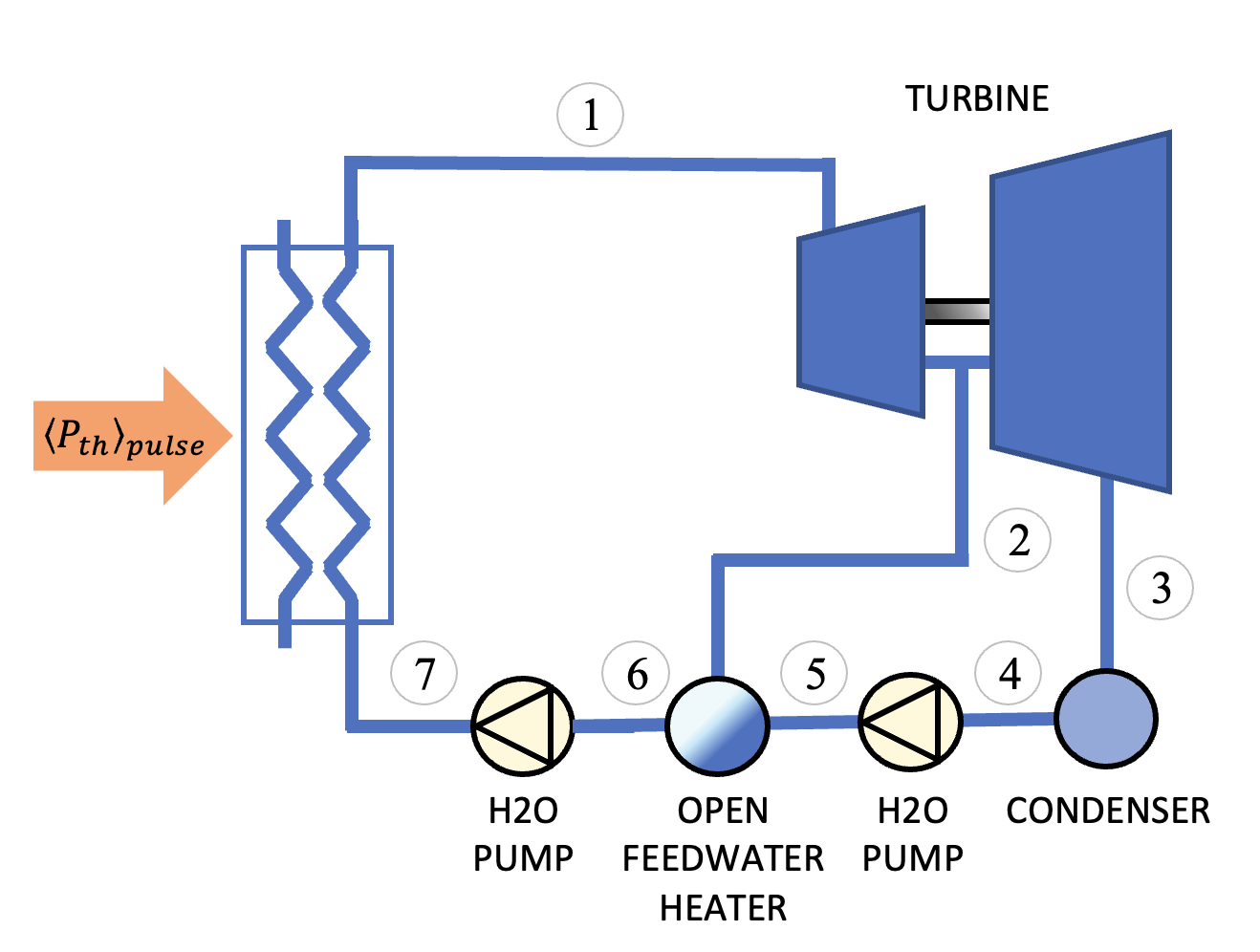
Figure 28: Diagram of Rankine cycle layout for sub and supercritical cycles. Heat from the secondary salt loop enters between states 7 and 1 as $\langle P_{th}\rangle_{pulse}$. A fraction of the working fluid is tapped at state 2, between high and low pressure turbine stages, for injection into the open feedwater heater. This reduces the total required pumping power.

State	Pressure [bar]		Temperature [°C]
	Sub	Super	Sub	Super
1	150	300	560	560
2	23	52	292	297
3	0.6	0.6	86	86
4	0.6	0.6	86	86
5	23	52	86	86
6	23	52	220	266
7	150	300	223	274

Table 10: Thermodynamic states for final subcritical and supercritical H${}_{\text{2}}$O Rankine cycles. State labels correspond to those presented in figure 28. Note that the temperature at state 5 is slightly higher than at state 4, but this has been obscured during rounding.

B.2 Thermodynamic Analysis of Brayton Cycle

A diagram of the Brayton cycle plant layout is presented in figure 29. A full list of the thermodynamic states used in the final analysis is provided in table 11. During analysis, all components were assumed to have an isentropic efficiency, $\eta_{s}=0.95$. The compressor is mounted directly to the turbine output shaft, and thus does not have an associated electrical efficiency. The optimized compression ratio, $p_{4}/p_{3}=2.1$. Finally, the regeneration efficacy is assumed to be $\eta_{regen}=0.8$.

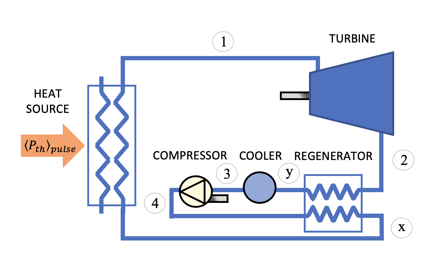
Figure 29: Diagram of Brayton cycle layout. Heat from the secondary salt loop enters between states 7 and x as $\langle P_{th}\rangle_{pulse}$. After exiting the turbine, Helium retains higher temperature than the compressor entrance, so it can be used for regeneration via a heat exchanger with outlet states x and y. For a given compression ratio, $p_{4}/p_{3}$, and maximum temperature, $T_{1}$, this reduces the amount of thermal power required to reach the same output power. Equivalently, this increases thermal efficiency of the cycle. Although not depicted here, the compressor can be mounted on the turbine shaft, so mechanical power can be directly tapped without intermediary losses due to electrical conversion.

State	Pressure [bar]	Temperature [°C]
1	2.1	560
2	1.0	372
3	1.0	27
4	2.1	27
x	2.1	325

Table 11: Thermodynamic states for final helium Brayton cycle. The working fluid is treated as an ideal gas. State labels correspond to those presented in figure 29.

Appendix C Economic Analysis

C.1 Overnight Costing Methods

Table 12: Reactor plant

Component	Cost (US$M)	Costing Method
Toroidal Field Coils	1,500	Broken into tape, support structure, resistive lead, and power supply costs. A fabrication factor of 3x was applied to the support structure, and fabrication factor of 5x was applied to the REBCO tape and resistive leads. Inconel 718 used for structural supports. Necessary tape length and structural support materials were calculated by treating the magnets as a rectangle with rounded corners.
Poloidal Field Coils	180	Broken into tape and support structure cost. A fabrication factor of 3x was applied to the support structure, and fabrication factor of 5x was applied to the REBCO tape. Nitronic 60 was used for structural supports.
Central Solenoid	140	Broken into tape and support structure cost. A fabrication factor of 3x was applied to the support structure, and fabrication factor of 5x was applied to the REBCO tape. Nitronic 60 was used for structural supports.
Cryosystem	110	Cryostat modeled as a 316 stainless steel cylinder containing the toroidal field coils. Its mass is scaled to ITER’s, using the ratio of their surface areas[151, 152]. For the cryocoolers, $ 1M / kW was assumed for a total of $90M [153].
Remote Maintenance	55	Value of contract for ITER’s remote maintenance system  [154]. The design of a such a system for a fusion power plant is very uncertain; this would be a valuable area for future research.
Plasma Heating	370	A cost of $10M / MW was assumed for the ICRH system.
Divertor	150	Estimation based on previous devices.
Vacuum Vessel	23	Vacuum vessel modeled as two concentric rectangles of V-4Cr-4Ti, with rounded corners, and a fabrication factor of 3x.
Diagnostics	100	Extrapolated from existing radiation hardened diagnostics.
Blanket	380	Blanket geometry modeled as shells. Tank is made of Cr-V steel and filled with FLiBe. Thermal shielding and neutron shielding use Boron Carbide and Titanium Carbide respectively. Solid layers have a fabrication factor of 3x.
Tritium	57	Assumed $30M for tritium handling system [138]. For start up inventory of 900g, a cost of $30,000/g was taken[155].

Table 13: Direct costs

Item	Cost (US$M)	Costing Method
Reactor equipment		Sum from table 12.
Turbine plant	200	Inflation-corrected estimate for power generation using a first of a kind, 350MWt, Rankine cycle on a high temperature gas cooled reactor [140]. Assumed interpulse storage costs are $25/kWh [156], resulting in a negligible additional cost. Estimate is conservative w.r.t a small fission reactor[157].
Electric plant	35	CBS 24 in [138].
Misc plant	17	CBS 25 in [138].
Heat rejection	11	CBS 26 in [138].
Land	15	CBS 20 in [138].
Structures	110	CBS 21 in [138].

Table 14: Indirect costs

Item	Cost (US$M)	Costing Method
Construction services	75	CBS 91 in [138].
Home office engineering	18	CBS 92 in [138].
Field office engineering	38	CBS 93 in [138].
Owner’s costs	18	CBS 94 in [138].

C.2 Materials Costs

Table 15: Material costs

Component	Cost	Component	Cost
REBCO	$ 40/kAm [assumed]	Titanium Carbide	$85/kg [158]
TF Power Supply	$0.5M/supply [159]	Stainless steel 316	$6.5 /kg[160]
TF Resistive Lead	$2 M/lead [assumed]	Inconel 718	$65/kg [161]
Deuterium	$21/g [162]	Nitronic 60	$25/kg [163]
Tritium	$30k/g [164]	Cr-V Steel	$43/kg [165]
FLiBe	$169/kg [19]
Boron Carbide	$142/kg [158]

C.3 Operational Costing: LCOE Terms

Table 16: Operational costs

Cost	Quantity and Calculation Method
Financing	A 3% interest rate, 3% inflation, 0% down-payment, and that the entire loan for the capital cost (including plant, facilities, and decommissioning) is payed off by the end of the project was assumed.
Taxes & Tax Credits	Taxes paid or tax credits received vary too much by location to be usefully included. Note that MANTA would likely be eligible for a nontrivial value of production tax credits such as under the Inflation Reduction Act[144], at time of publication.
Personnel Costs	15$M/yr = ($\sim$1 person/MWe)$\times$$150,000/(employee-year) [166]
Yearly Capital Repairs	0.5% of capital cost + 1 vacuum vessel every two years (including fabrication and removal/installation) due to radiation damage.
Magnet Replacement	It was assumed that only the REBCO portion of the magnet requires replacement due to radiation damage, and the replacement times (see table 7) are grouped to the nearest half-year to decrease the number of zero-production maintenance months. A 2 month maintenance downtime was assumed, and a REBCO replacement cost ranging from $853M for the TF magnet to $20.9M-$36.9M for the PFs.
Fueling Costs	After a 900g startup inventory, fueling is defined as a negative cost due to selling tritium at an assumed current price of $30k/g[164].
Electricity Cost	$47.6/MWhr[167] is used as the US east coast wholesale marginal price for selling electricity.
Power Production	An effective duty cycle of 90% was calculated due to recharging the thermal reservoir to maintain constant electrical producing during CS swings, a further 88% for plant availability due to maintenance downtime (2 month per magnet replacement), 36% for turbine efficiency, and 95% for each of the four Heat Exchangers (not always simultaneously in use, see Fig. 22). Disruptivity and uncontrolled shutdowns are not included in the analysis (other works have investigated these effects on plant economic viability[108]). Total thermal power is calculated in Sec. 6.
Power Consumption	Electrical consumption consists of auxiliary heating (40 MW at a wall-plug efficiency of 70%), cryostat (1.5 MW[168]), turbine and FLiBe pump (4.88 MW), and diagnostic systems (0.1 MW).

References

- [1] National Academy of Engineering and National Academies of Sciences, Engineering, and Medicine “Bringing Fusion to the U.S. Grid” Washington, DC: The National Academies Press, 2021 DOI: 10.17226/25991
- [2] M. Diez et al. “In situ observation of tungsten plasma-facing components after the first phase of operation of the WEST tokamak” In Nuclear Fusion 61.10 IOP Publishing, 2021, pp. 106011 DOI: 10.1088/1741-4326/ac1dc6
- [3] A Huber et al. “Understanding tungsten erosion during inter/intra-ELM periods in He-dominated JET-ILW plasmas” In Physica Scripta 96.12 IOP Publishing, 2021, pp. 124046 DOI: 10.1088/1402-4896/ac2d85
- [4] X. Litaudon et al. “Long plasma duration operation analyses with an international multi-machine (tokamaks and stellarators) database” In Nuclear Fusion 64.1 IOP Publishing, 2023, pp. 015001 DOI: 10.1088/1741-4326/ad0606
- [5] A.. Kuang et al. “Divertor heat flux challenge and mitigation in SPARC” In Journal of Plasma Physics 86.5, 2020, pp. 865860505 DOI: 10.1017/S0022377820001117
- [6] J.E. Menard et al. “Fusion pilot plant performance and the role of a sustained high power density tokamak” In Nuclear Fusion 62.3, 2022, pp. 036026 DOI: 10.1088/1741-4326/ac49aa
- [7] D.N. Hill “A review of ELMs in divertor tokamaks” In Journal of Nuclear Materials 241-243, 1997, pp. 182–198 DOI: https://doi.org/10.1016/S0022-3115(97)80039-6
- [8] R.P. Wenninger et al. “DEMO divertor limitations during and in between ELMs” In Nuclear Fusion 54.11 IOP Publishing, 2014, pp. 114003 DOI: 10.1088/0029-5515/54/11/114003
- [9] C Paz-Soldan and DIII-D Team “Plasma performance and operational space without ELMs in DIII-D” In Plasma Physics and Controlled Fusion 63.8 IOP Publishing, 2021, pp. 083001 DOI: 10.1088/1361-6587/ac048b
- [10] E. Viezzer et al. “Prospects of core–edge integrated no-ELM and small-ELM scenarios for future fusion devices” In Nuclear Materials and Energy 34, 2023, pp. 101308 DOI: https://doi.org/10.1016/j.nme.2022.101308
- [11] T C Luce “An analytic functional form for characterization and generation of axisymmetric plasma boundaries” In Plasma Physics and Controlled Fusion 55.9 IOP Publishing, 2013, pp. 095009 DOI: 10.1088/0741-3335/55/9/095009
- [12] A.O. Nelson, C. Paz-Soldan and S. Saarelma “Prospects for H-mode inhibition in negative triangularity tokamak reactor plasmas” In Nuclear Fusion 62.9 IOP Publishing, 2022, pp. 096020 DOI: 10.1088/1741-4326/ac8064
- [13] A.. Nelson et al. “Robust Avoidance of Edge-Localized Modes alongside Gradient Formation in the Negative Triangularity Tokamak Edge” In Phys. Rev. Lett. 131 American Physical Society, 2023, pp. 195101 DOI: 10.1103/PhysRevLett.131.195101
- [14] M.. Austin et al. “Achievement of Reactor-Relevant Performance in Negative Triangularity Shape in the DIII-D Tokamak” In Phys. Rev. Lett. 122 American Physical Society, 2019, pp. 115001 DOI: 10.1103/PhysRevLett.122.115001
- [15] M. Kikuchi, A. Fasoli and T Takizuka “Negative Triangularity Tokamak as Fusion Energy System” In [Proceedings] 1st International e-Conference on Energies, 2014 DOI: 10.3390/ece-1-e002
- [16] S Yu Medvedev et al. “Single null divertor in negative triangularity tokamak” In 26th IAEA Fusion Energy Conference, 2016, pp. 17–22
- [17] M. Kikuchi et al. “L-mode-edge negative triangularity tokamak reactor” In Nuclear Fusion 59.5 IOP Publishing, 2019, pp. 056017 DOI: 10.1088/1741-4326/ab076d
- [18] S.Yu. Medvedev et al. “The negative triangularity tokamak: stability limits and prospects as a fusion energy system” In Nuclear Fusion 55.6 IOP Publishing, 2015, pp. 063013 DOI: 10.1088/0029-5515/55/6/063013
- [19] B.N. Sorbom et al. “ARC: A compact, high-field, fusion nuclear science facility and demonstration power plant with demountable magnets” In Fusion Engineering and Design 100, 2015, pp. 378–405 DOI: https://doi.org/10.1016/j.fusengdes.2015.07.008
- [20] T. Carter et al. “Powering the Future: Fusion and Plasmas”, 2020
- [21] S Coda et al. “Enhanced confinement in diverted negative-triangularity L-mode plasmas in TCV” In Plasma Physics and Controlled Fusion 64.1 IOP Publishing, 2021, pp. 014004 DOI: 10.1088/1361-6587/ac3fec
- [22] A. Marinoni, M.E. Austin and A.W. Hyatt “Diverted negative triangularity plasmas on DIII-D: the benefit of high confinement without the liability of an edge pedestal” In Nuclear Fusion 61.11 IOP Publishing, 2021, pp. 116010 DOI: 10.1088/1741-4326/ac1f60
- [23] A. Marinoni, M.. Austin and A.. Hyatt “H-mode grade confinement in L-mode edge plasmas at negative triangularity on DIII-D” In Physics of Plasmas 26.4, 2019, pp. 042515 DOI: 10.1063/1.5091802
- [24] C. Paz-Soldan et al. “Simultaneous access to high normalized current, pressure, density, and confinement in strongly-shaped diverted negative triangularity plasmas”, 2023 DOI: https://doi.org/10.48550/arXiv.2309.03689
- [25] Y. Camenen et al. “Impact of plasma triangularity and collisionality on electron heat transport in TCV L-mode plasmas” In Nuclear Fusion 47.7, 2007, pp. 510 DOI: 10.1088/0029-5515/47/7/002
- [26] M. Fontana et al. “Effects of collisionality and Te/Ti on fluctuations in positive and negative tokamak plasmas” In Nuclear Fusion 60.1 IOP Publishing, 2019, pp. 016006 DOI: 10.1088/1741-4326/ab4d75
- [27] W.A. Houlberg, S.E. Attenberger and L.M. Hively “Contour analysis of fusion reactor plasma performance” In Nuclear Fusion 22.7, 1982, pp. 935 DOI: 10.1088/0029-5515/22/7/006
- [28] D.J. Battaglia et al. “cfs-energy/cfspopcon: v4.0.0” Zenodo, 2023 DOI: 10.5281/ZENODO.10054879
- [29] S.J. Frank et al. “Radiative pulsed L-mode operation in ARC-class reactors” In Nuclear Fusion 62.12 IOP Publishing, 2022, pp. 126036 DOI: 10.1088/1741-4326/ac95ac
- [30] C. Angioni et al. “Relationship between density peaking, particle thermodiffusion, Ohmic confinement, and microinstabilities in ASDEX Upgrade L-mode plasmas” In Physics of Plasmas 12.4, 2005, pp. 040701 DOI: 10.1063/1.1867492
- [31] ITER Physics Expert Group on Confinement and Transport, ITER Physics Expert Group on Confinement Modelling and Database and ITER Physics Basis Editors “Chapter 2: Plasma confinement and transport” In Nuclear Fusion 39.12, 1999, pp. 2175 DOI: 10.1088/0029-5515/39/12/302
- [32] A.. Creely et al. “Overview of the SPARC tokamak” In Journal of Plasma Physics 86.5, 2020, pp. 865860502 DOI: 10.1017/S0022377820001257
- [33] J.. Menard et al. “Aspect ratio scaling of ideal no-wall stability limits in high bootstrap fraction tokamak plasmas” In Physics of Plasmas 11.2, 2004, pp. 639–646 DOI: 10.1063/1.1640623
- [34] J.. Freidberg, A. Cerfon and J. Lee “Tokamak elongation – how much is too much? Part 1. Theory” In Journal of Plasma Physics 81.6, 2015, pp. 515810607 DOI: 10.1017/S0022377815001270
- [35] Junhyuk Song, Carlos Paz-Soldan and Jungpyo Lee “Impact of negative triangularity plasma shaping on the n = 0 resistive wall mode in a tokamak” In Nuclear Fusion 61.9, 2021, pp. 096033 DOI: 10.1088/1741-4326/ac189a
- [36] A O Nelson et al. “Vertical control of DIII-D discharges with strong negative triangularity” In Plasma Physics and Controlled Fusion 65.4 IOP Publishing, 2023, pp. 044002 DOI: 10.1088/1361-6587/acbe65
- [37] S. Guizzo et al. “Assessment of vertical stability for negative triangularity pilot plants”, 2024 arXiv:2401.15217 [physics.plasm-ph]
- [38] Paul K. Romano et al. “OpenMC: A state-of-the-art Monte Carlo code for research and development” Joint International Conference on Supercomputing in Nuclear Applications and Monte Carlo 2013, SNA + MC 2013. Pluri- and Trans-disciplinarity, Towards New Modeling and Numerical Simulation Paradigms In Annals of Nuclear Energy 82, 2015, pp. 90–97 DOI: https://doi.org/10.1016/j.anucene.2014.07.048
- [39] H. Lütjens, A. Bondeson and O. Sauter “The CHEASE code for toroidal MHD equilibria” In Computer Physics Communications 97.3, 1996, pp. 219–260 URL: https://doi.org/10.1016/0010-4655(96)00046-X
- [40] J. Candy et al. “Tokamak profile prediction using direct gyrokinetic and neoclassical simulation” In Physics of Plasmas 16.6, 2009, pp. 060704 URL: https://doi.org/10.1063/1.3167820
- [41] T.H. Stix “Fast-wave heating of a two-component plasma” In Nuclear Fusion 15.5, 1975, pp. 737 DOI: 10.1088/0029-5515/15/5/003
- [42] Y. Lin, J.. Wright and S. Wukitch “Physics basis for the ICRF system of the SPARC tokamak” In Journal of Plasma Physics 86.5, 2020 DOI: 10.1017/S0022377820001269
- [43] J. Irby et al. “Alcator C-Mod Design, Engineering, and Disruption Research” In Fusion Science and Technology 51.3 Taylor & Francis, 2007, pp. 460–475 DOI: 10.13182/FST07-A1433
- [44] O. Meneghini et al. “Neural-network accelerated coupled core-pedestal simulations with self-consistent transport of impurities and compatible with ITER IMAS” In Nuclear Fusion 61.2 IAEA, 2020 DOI: 10.1088/1741-4326/abb918
- [45] O. Meneghini et al. “Integrated modeling applications for tokamak experiments with OMFIT” In Nuclear Fusion 55.8 IOP Publishing, 2015, pp. 083008 DOI: 10.1088/0029-5515/55/8/083008
- [46] T. Slendebroek et al. “Elevating zero dimensional global scaling predictions to self-consistent theory-based simulations” In Physics of Plasmas 30.7, 2023, pp. 072511 DOI: 10.1063/5.0148886
- [47] R.L. Miller et al. “Stable equilibria for bootstrap-current-driven low aspect ratio tokamaks” In Physics of Plasmas 4, 1997, pp. 1062–1068 DOI: 10.1063/1.872193
- [48] M. Brambilla “Numerical simulation of ion cyclotron waves in tokamak plasmas” In Plasma Physics and Controlled Fusion 41.1, 1999 DOI: 10.1088/0741-3335/41/1/002
- [49] RW Harvey and MG McCoy “The CQL3D fokker-planck code” In Proceedings of the IAEA Technical Committee Meeting on Simulation and Modeling of Thermonuclear Plasmas, 1992, pp. 489–526
- [50] B.. Lyons et al. “Flexible, integrated modeling of tokamak stability, transport, equilibrium, and pedestal physics” In Physics of Plasmas 30.9, 2023, pp. 092510 DOI: 10.1063/5.0156877
- [51] E.A. Belli and J. Candy “An Eulerian method for the solution of the multi-species drift-kinetic equation” In Plasma Physics and Controlled Fusion 51.7, 2009 DOI: 10.1088/0741-3335/51/7/075018
- [52] G. Staebler, J. Kinsey and R. Waltz “A theory-based transport model with comprehensive physics” In Physics of Plasmas 14, 2007, pp. 055909–055909 DOI: 10.1063/1.2436852
- [53] C. Angioni et al. “Scaling of density peaking in H-mode plasmas based on a combined database of AUG and JET observations” In Nuclear Fusion 47.9, 2007, pp. 1326 DOI: 10.1088/0029-5515/47/9/033
- [54] P. Rodriguez-Fernandez, N.T. Howard and J. Candy “Nonlinear gyrokinetic predictions of SPARC burning plasma profiles enabled by surrogate modeling” In Nuclear Fusion 62.7 IOP Publishing, 2022, pp. 076036 DOI: 10.1088/1741-4326/ac64b2
- [55] Sam Frank “Simulating energetic ions and enhanced neutron rates from ion-cyclotron resonance heating with a new fast, self-consistent full-wave + Fokker-Planck model” 65th Annual Meeting of the APS Division of Plasma Physics, 2023 URL: https://meetings.aps.org/Meeting/DPP23/Session/KI02.4
- [56] G M Staebler et al. “Geometry dependence of the fluctuation intensity in gyrokinetic turbulence” In Plasma Physics and Controlled Fusion 63.1 IOP Publishing, 2020, pp. 015013 DOI: 10.1088/1361-6587/abc861
- [57] G.M. Staebler et al. “Verification of a quasi-linear model for gyrokinetic turbulent transport” In Nuclear Fusion 61.11 IOP Publishing, 2021, pp. 116007 DOI: 10.1088/1741-4326/ac243a
- [58] J. McClenaghan In Plasma Physics and Controlled Fusion IOP Publishing, 2024, pp. In this issue
- [59] M. Greenwald “Density limits in toroidal plasmas” In Plasma Physics and Controlled Fusion 44.8, 2002 DOI: 10.1088/0741-3335/44/8/201
- [60] P. Rodriguez-Fernandez et al. “Enhancing predictive capabilities in fusion burning plasmas through surrogate-based optimization in core transport solvers”, 2023 arXiv:2312.12610 [physics.plasm-ph]
- [61] B. LaBombard et al. “ADX: a high field, high power density, advanced divertor and RF tokamak” In Nuclear Fusion 55.5 IOP Publishing, 2015, pp. 053020 DOI: 10.1088/0029-5515/55/5/053020
- [62] R. Kembleton, M. Siccinio, F. Mavigalia and F. Militello “Benefits and Challenges of Advanced Divertor Configurations in DEMO” In Fusion Engineering and Design 179, 2022, pp. 113120 DOI: 10.1016/j.fusengdes.2022.113120
- [63] M.R.K. Wigram et al. “Performance assessment of long-legged tightly-baffled divertor geometries in the ARC reactor concept” In Nuclear Fusion 59.10 IOP Publishing, 2019, pp. 106052 DOI: 10.1088/1741-4326/ab394f
- [64] T. Eich et al. “Scaling of the tokamak near the scrape-off layer H-mode power width and implications for ITER” In Nuclear Fusion 53.9, 2013, pp. 093031 DOI: 10.1088/0029-5515/53/9/093031
- [65] D. Moulton, P.C. Stangeby, X. Bonnin and R.A. Pitts “Comparison between SOLPS-4.3 and the Lengyel Model for ITER baseline neon-seeded plasmas” In Nuclear Fusion 61.4, 2021, pp. 046029 DOI: 10.1088/1741-4326/abe4b2
- [66] B. Sorbom, A. Creely and C. Tse “Recent developments in the design of ARC” In 62nd Annual Meeting of the APS Division of Plasma Physics, 2020
- [67] G. Zhuang et al. “Progress of the CFETR design” In Nuclear Fusion 59.11, 2019, pp. 112010 DOI: 10.1088/1741-4326/ab0e27
- [68] H. Reimerdes et al. “Assessment of alternative divertor configurations as an exhaust solution for DEMO” In Nuclear Fusion 60.6, 2020, pp. 066030 DOI: 10.1088/1741-4326/ab8a6a
- [69] B D Dudson “FreeGS”, 2023 URL: https://github.com/freegs-plasma/freegs
- [70] N. de Boucaud, T. Golfinopoulos and A. Marinoni “Demonstration and evaluation of negative triangularity equilibria in the ARC fusion pilot plant concept” In Fusion Engineering and Design 202, 2024, pp. 114401 DOI: https://doi.org/10.1016/j.fusengdes.2024.114401
- [71] T.D. Rognlien, J.L. Milovich, M.E. Rensink and G.D. Porter “A fully implicit, time dependent 2-D fluid code for modeling tokamak edge plasmas” In Journal of Nuclear Materials 196-198, 1992, pp. 347–351 DOI: 10.1016/S0022-3115(06)80058-9
- [72] S.B. Ballinger et al. “Simulation of the SPARC plasma boundary with the UEDGE code” In Nuclear Fusion 61 IOP Publishing, 2021, pp. 086014 DOI: 10.1088/1741-4326/ac0c2f
- [73] A Loarte et al. “Plasma detachment in JET Mark I divertor experiments” In Nuclear Fusion 38.3, 1998, pp. 331–371 DOI: 10.1088/0029-5515/38/3/303
- [74] A.W. Leonard et al. “Scaling radiative divertor solutions to high power in DIII-D” In Nuclear Fusion 52.6, 2012, pp. 063015 DOI: 10.1088/0029-5515/52/6/063015
- [75] A Kallenbach et al. “Impurity seeding for tokamak power exhaust: from present devices via ITER to DEMO” In Plasma Physics and Controlled Fusion 55.12, 2013, pp. 124041 DOI: 10.1088/0741-3335/55/12/124041
- [76] F Sciortino, N T Howard and T Odstrčil “Investigation of core impurity transport in DIII-D diverted negative triangularity plasmas” In Plasma Physics and Controlled Fusion 64.12 IOP Publishing, 2022, pp. 124002 DOI: 10.1088/1361-6587/ac94f6
- [77] T. Eich et al. “Empiricial scaling of inter-ELM power widths in ASDEX Upgrade and JET” In Journal of Nuclear Materials 438, 2013, pp. S72–S77 DOI: 10.1016/j.jnucmat.2013.01.011
- [78] D. Brunner, B. LaBombard, A.Q. Kuang and J.L. Terry “High-resolution heat flux width measurements at reactor-level magnetic fields and observation of a unified width scaling across confinement regimes in the Alcator C-Mod tokamak” In Nuclear Fusion 58.9, 2018, pp. 094002 DOI: 10.1088/1741-4326/aad0d6
- [79] J. Horacek, J. Adamek and M. Komm “Scaling of L-mode heat flux for ITER and COMPASS-U divertors, based on five tokamaks” In Nuclear Fusion 60.6, 2020, pp. 066016 DOI: 10.1088/1741-4326/ab7e47
- [80] M Faitsch et al. “Dependence of the L-Mode scrape-off layer power fall-off length on the upper triangularity in TCV” In Plasma Physics and Controlled Fusion 60.4, 2018, pp. 045010 DOI: 10.1088/1361-6587/aaaef7
- [81] F. Scotti In Plasma Physics and Controlled Fusion IOP Publishing, 2024, pp. In this issue
- [82] B. LaBombard et al. “Particle transport in the scrape-off layer and its relationship to discharge density limit in Alcator C-Mod” In Physics of Plasmas 8.5, 2001, pp. 2107–2117 DOI: 10.1063/1.1352596
- [83] D. Brunner, A.Q. Kuang, B. LaBombard and J.L. Terry “The dependence of divertor power sharing on magnetic flux balance in near double-null configurations on Alcator C-Mod” In Nuclear Fusion 58.7 IOP Publishing, 2018, pp. 076010 DOI: 10.1088/1741-4326/aac006
- [84] G. Temmerman et al. “Thermographic study of heat load asymmetries during MAST L-mode discharges” In Plasma Physics and Controlled Fusion 52.9 IOP Publishing, 2010, pp. 095005 DOI: 10.1088/0741-3335/52/9/095005
- [85] K. Lim et al. “Effect of triangularity on plasma turbulence and the SOL-width scaling in L-mode diverted tokamak configurations” In Nuclear Fusion 65.8 IOP Publishing, 2023, pp. 085006 DOI: 10.1088/1361-6587/acdc52
- [86] S.B. Ballinger et al. “Dependence of the boundary heat flux width on core and edge profiles in Alcator C-Mod” In Nuclear Fusion 62.7 IOP Publishing, 2022, pp. 076020 DOI: 10.1088/1741-4326/ac637c
- [87] D. Silvagni et al. “Scrape-off layer (SOL) power width scaling and correlation between SOL and pedestal gradients across L, I and H-mode plasmas at ASDEX Upgrade” In Nuclear Fusion 62.4 IOP Publishing, 2020, pp. 045015 DOI: 10.1088/1361-6587/ab74e8
- [88] D.L. Hillis et al. “Noble gas impurity balance and exhaust model for DIII-D and JET” In Journal of Nuclear Materials 266-269 Elsevier, 1999, pp. 1084–1090 DOI: 10.1016/S0022-3115(98)00563-7
- [89] T Hirai et al. “ITER full tungsten divertor qualification program and progress” In Physica Scripta T159, 2014, pp. 014006 DOI: 10.1088/0031-8949/2014/T159/014006
- [90] J.N. Brooks “Analysis of tungsten migration from the C-MOD divertor; prediction of high redeposition rate, and code validation progress” In Nuclear Fusion 53.4, 2013, pp. 042001 DOI: 10.1088/0029-5515/53/4/042001
- [91] S. al Brezinsek “Erosion, screening, and migration of tungsten in the JET divertor” In Nuclear Fusion 59.9, 2019, pp. 096035 DOI: 10.1088/1741-4326/ab2aef
- [92] D. Hwangbo, S. Kawaguchi, S. Kajita and N. Ohno “Erosion of nanostructured tungsten by laser ablation, sputtering and arcing” In Nuclear Materials and Energy 12, 2017, pp. 386–391 DOI: 10.1016/j.nme.2017.03.004
- [93] D.S. Meluzova, P.Yu. Babenko, A.N. Zinoviev and A.P. Shergin “Sputtering of Tungsten by Beryllium and Neon Ions” In Technical Physics Letters 46.12, 2020, pp. 1227–1230 DOI: 10.1134/S1063785020120226
- [94] X. al Zhao “The erosion of tungsten divertor on EAST during neon impurity seeding in different divertor operation regimes” In Plasma Physics and Controlled Fusion 62, 2020, pp. 055015 DOI: 10.1088/1361-6587/ab831b
- [95] Ansys inc. “Ansys Fluent”, 2024 URL: https://www.ansys.com/products/fluids/ansys-fluent
- [96] A. Suslova et al. “Recrystallization and grain growth induced by ELMs-like transient heat loads in deformed tungsten samples” In Sci Rep 4, 2014, pp. 6845 DOI: 10.1038/srep06845
- [97] Zachary S. Hartwig, Rui F. Vieira, Darby Dunn and Theodore Golfinopoulos “The SPARC Toroidal Field Model Coil Program” In IEEE Transactions on Applied Superconductivity 34.2, 2024, pp. 1–16 DOI: 10.1109/TASC.2023.3332613
- [98] Rui F. Vieira et al. “Design, Fabrication, and Assembly of the SPARC Toroidal Field Model Coil” In IEEE Transactions on Applied Superconductivity 34.2, 2024, pp. 1–15 DOI: 10.1109/TASC.2024.3356571
- [99] D.. Whyte et al. “Experimental Assessment and Model Validation of the SPARC Toroidal Field Model Coil” In IEEE Transactions on Applied Superconductivity 34.2, 2024, pp. 1–18 DOI: 10.1109/TASC.2023.3332823
- [100] Zachary S Hartwig et al. “VIPER: an industrially scalable high-current high-temperature superconductor cable” In Superconductor Science and Technology 33.11 IOP Publishing, 2020, pp. 11LT01 DOI: 10.1088/1361-6668/abb8c0
- [101] J. File, R.. Mills and G.. Sheffield “Large Superconducting Magnet Designs for Fusion Reactors” In IEEE Transactions on Nuclear Science 18.4, 1971, pp. 277–282 DOI: 10.1109/TNS.1971.4326354
- [102] W. Beck “Alcator C-MOD toroidal field magnet assembly” In [Proceedings] The 14th IEEE/NPSS Symposium Fusion Engineering, 1991, pp. 292–294 vol.1 DOI: 10.1109/FUSION.1991.218896
- [103] COMSOL AB “COMSOL Multiphysics®”, 2023 URL: www.comsol.com
- [104] R.L. Tobler “Low temperature effects on the fracture behaviour of a nickel base superalloy” In Cryogenics 16.11, 1976, pp. 669–674 DOI: https://doi.org/10.1016/0011-2275(76)90039-4
- [105] A. Molodyk, S. Samoilenkov and A. Markelov “Development and large volume production of extremely high current density YBa2Cu3O7 superconducting wires for fusion” In Scientific Reports 11.1 Nature Publishing Group UK, 2021, pp. 1–11 DOI: 10.1038/s41598-021-81559-z
- [106] Theodore Mouratidis, Dennis G Whyte, Brian LaBombard and William K Beck “Performance of demountable solder joints for no-insulation superconducting coils produced by vacuum pressure impregnation” In Superconductor Science and Technology 37.2 IOP Publishing, 2024, pp. 025006 DOI: 10.1088/1361-6668/ad0b2b
- [107] Theodore Mouratidis “Low Temperature Solder Demountable Joints for Non-Insulated, High Temperature Superconducting Fusion Magnets”, 2022
- [108] Andrew D. Maris et al. “The Impact of Disruptions on the Economics of a Tokamak Power Plant” In Fusion Science and Technology 0.0 Taylor & Francis, 2023, pp. 1–17 DOI: 10.1080/15361055.2023.2229675
- [109] A. Tesini and J. Palmer “The ITER remote maintenance system” Proceedings of the Eight International Symposium of Fusion Nuclear Technology In Fusion Engineering and Design 83.7, 2008, pp. 810–816 DOI: https://doi.org/10.1016/j.fusengdes.2008.08.011
- [110] Y. Chu et al. “Estimation of Operational Stability for the KSTAR TF Magnet” In IEEE Transactions on Applied Superconductivity 21.3, 2011, pp. 2004–2007 DOI: 10.1109/TASC.2011.2107870
- [111] “PRIS - Trend reports - Unplanned Capability Loss” URL: https://pris.iaea.org/PRIS/WorldStatistics/WorldTrendinUnplannedCapabilityLossFactor.aspx
- [112] H.‐S. Chang et al. “OPERATION RESULTS OF THE KSTAR HELIUM REFRIGERATION SYSTEM” In AIP Conference Proceedings 1218.1, 2010, pp. 1476–1483 DOI: 10.1063/1.3422326
- [113] N. Peng, L.Q. Liu and L.Y. Xiong “Thermal–hydraulic analysis of the cool-down for the ITER magnets” In Cryogenics 57, 2013, pp. 45–49 DOI: https://doi.org/10.1016/j.cryogenics.2013.05.002
- [114] Franco Julio Mangiarotti “An experimental device for critical surface characterization of YBCO tape superconductors”, 2013
- [115] Masayoshi SUGIHARA et al. “Plasma Design Considerations of Near Term Tokamak Fusion Experimental Reactor” In Journal of Nuclear Science and Technology 19.8 Taylor & Francis, 1982, pp. 628–637 DOI: 10.1080/18811248.1982.9734193
- [116] C. Barth, G. Mondonico and C. Senatore “Electro-mechanical properties of REBCO coated conductors from various industrial manufacturers at 77 K, self-field and 4.2 K, 19 T” Publisher: IOP Publishing In Superconductor Science and Technology 28.4, 2015, pp. 045011 DOI: 10.1088/0953-2048/28/4/045011
- [117] B. Sorbom et al. “Liquid immersion blanket design for use in a compact modular fusion reactor” In Bulletin of the American Physical Society 57, 2012 URL: https://meetings.aps.org/Meeting/DPP12/Event/176631
- [118] DK SZE “IPFR, INTEGRATED POOL FUSION-REACTOR CONCEPT” In FUSION TECHNOLOGY 10.3, 2A, 1986, pp. 875–880 DOI: 10.13182/FST86-A24847
- [119] Takeo Muroga “Vanadium Alloys for Fusion Blanket Applications” In MATERIALS TRANSACTIONS 46.3, 2005, pp. 405–411 DOI: 10.2320/matertrans.46.405
- [120] Steven J. Zinkle and Jeremy T. Busby “Structural materials for fission & fusion energy” In Materials Today 12.11, 2009, pp. 12–19 DOI: https://doi.org/10.1016/S1369-7021(09)70294-9
- [121] W R Meier “Multivariable optimization of fusion reactor blankets”, 1984 DOI: 10.2172/6745334
- [122] D X Fischer, R Prokopec, J Emhofer and M Eisterer “The effect of fast neutron irradiation on the superconducting properties of REBCO coated conductors with and without artificial pinning centers” In Superconductor Science and Technology 31.4 IOP Publishing, 2018, pp. 044006 DOI: 10.1088/1361-6668/aaadf2
- [123] R Prokopec, D X Fischer, H W Weber and M Eisterer “Suitability of coated conductors for fusion magnets in view of their radiation response” In Superconductor Science and Technology 28.1 IOP Publishing, 2014, pp. 014005 DOI: 10.1088/0953-2048/28/1/014005
- [124] M.B. Chadwick et al. “ENDF/B-VII.1 Nuclear Data for Science and Technology: Cross Sections, Covariances, Fission Product Yields and Decay Data” Special Issue on ENDF/B-VII.1 Library In Nuclear Data Sheets 112.12, 2011, pp. 2887–2996 DOI: 10.1016/j.nds.2011.11.002
- [125] M.J. Norgett, M.T. Robinson and I.M. Torrens “A proposed method of calculating displacement dose rates” In Nuclear Engineering and Design 33.1, 1975, pp. 50–54 DOI: https://doi.org/10.1016/0029-5493(75)90035-7
- [126] D.L. Smith et al. “Development of vanadium-base alloys for fusion first-wall—blanket applications” In Fusion Engineering and Design 29, 1995, pp. 399–410 DOI: https://doi.org/10.1016/0920-3796(95)80046-Z
- [127] D.L Smith, M.C Billone and K Natesan “Vanadium-base alloys for fusion first-wall/blanket applications” Refractory Metals and Alloys, 1999 TMS Fall Meeting In International Journal of Refractory Metals and Hard Materials 18.4, 2000, pp. 213–224 DOI: https://doi.org/10.1016/S0263-4368(00)00037-8
- [128] Samuele Meschini “SamueleMeschini/fuel-cycle: Submitted version” Zenodo, 2023 DOI: 10.5281/zenodo.8019892
- [129] Samuele Meschini, Sara E. Ferry, Rémi Delaporte-Mathurin and Dennis G. Whyte “Modeling and analysis of the tritium fuel cycle for ARC- and STEP-class D-T fusion power plants” In Nuclear Fusion 63.12 IOP Publishing, 2023, pp. 126005 URL: https://dx.doi.org/10.1088/1741-4326/acf3fc
- [130] M. Sohal, M. Ebner, Sabharwall P. and P. Sharpe “Engineering Database of Liquid Salt Thermophysical and Thermochemical Properties”, 2013
- [131] E. Matsuo, M. Tsutsumi and K. Ogata “Conceptual design of helium gas turbine for MHTGR-GT”, 1996
- [132] H.C. No, J.H. Kim and H.M. Kim “A Review of Helium Gas Turbine Technology for High-Temperature Gas-Cooled Reactors” In Nuclear Engineering and Technology 39.1, 2007, pp. 21–30 DOI: https://doi.org/10.5516/NET.2007.39.1.021
- [133] Black and Vetach “Power Plant Engineering” Kluwer Academic Publishers, 1996
- [134] M.J. Moran, H.N. Shapiro, D.D. Boettner and M.B. Bailey “Fundamentals of Engineering Thermodynamics 8th Edition” Wiley, 2014
- [135] drunsinn “pyXSteam” In GitHub repository GitHub, https://github.com/drunsinn/pyXSteam, 2023
- [136] C.. Martin “PYroMat” In GitHub repository GitHub, https://github.com/chmarti1/PYroMat, 2022
- [137] Federal Railroad Administration “Capital Costing Estimating”, 2016
- [138] Simon Woodruff et al. “Conceptual Cost Study for a Fusion Power Plant Based on Four Technologies from the DOE ARPA-E ALPHA Program” Publisher: Unpublished, 2017 DOI: 10.13140/RG.2.2.24116.55688
- [139] Dale M. Meade “A Comparison of Unit Costs for FIRE and ITER” 2002 Fusion Summer Study, 2002
- [140] “Assessment of High Temperature Gas-Cooled Reactor (HTGR) Capital and Operating Costs”, 2012
- [141] William Riggins “Think closing power plants is less risky than opening them? That’s a mistake — Utility Dive”, https://www.utilitydive.com/news/think-closing-power-plants-is-less-risky-than-opening-them-thats-a-mistak/559915/
- [142] White House “FACT SHEET: President Biden Sets 2030 Greenhouse Gas Pollution Reduction Target Aimed at Creating Good-Paying Union Jobs and Securing U.S. Leadership on Clean Energy Technologies”, https://www.whitehouse.gov/briefing-room/statements-releases/2021/04/22/fact-sheet-president-biden-sets-2030-greenhouse-gas-pollution-reduction-target-aimed-at-creating-good-paying-union-jobs-and-securing-u-s-leadership-on-clean-energy-technologies/, 2021
- [143] Joseph R. Biden ““Catalyzing Clean Energy Industries and Jobs Through Federal Sustainability””, Executive Order (EO) 14057, 2021
- [144] 117$^st$ Congress “H.R.5376 - Inflation Reduction Act of 2022”, 2022
- [145] Seth A. Hoedl “Achieving a social license for fusion energy” In Physics of Plasmas 29.9, 2022, pp. 092506 DOI: 10.1063/5.0091054
- [146] Office of Long-Term Energy Modeling “Electricity Market Module of the National Energy Modeling System: Model Documentation”, 2022
- [147] E. Rubin et al. “Towards improved cost guidelines for advance low-carbon technologies” In 15th International Conference of Greenhouse Gas Control TEchnologies, 2021
- [148] Richard J. Pearson, Armando B. Antoniazzi and William J. Nuttall “Tritium supply and use: a key issue for the development of nuclear fusion energy” Special Issue: Proceedings of the 13th International Symposium on Fusion Nuclear Technology (ISFNT-13) In Fusion Engineering and Design 136, 2018, pp. 1140–1148 DOI: https://doi.org/10.1016/j.fusengdes.2018.04.090
- [149] “Levelized Costs of New Generation Resources in the Annual Energy Outlook”, 2022
- [150] Young-Gyun Kim et al. “Numerical analysis on bifurcated current flow in no-insulation magnet” In IEEE transactions on applied superconductivity 24.3 IEEE, 2013, pp. 1–4
- [151] ITER Organization “Cryostat”, http://www.iter.org/mach/cryostat
- [152] ITER Organization “Magnets”, https://www.iter.org/mach/Magnets
- [153] T. Golfinopolous, private communication, 2022
- [154] World Nuclear News “Contract for Iter remote handling system”, https://www.world-nuclear-news.org/Articles/Contract-for-Iter-remote-handling-system
- [155] M. Coleman and M. Kovari “Global supply of tritium for fusion R&D” In 27th IAEA Fusion Energy Conference, 2018
- [156] Charles Forsberg, private communication, 2022
- [157] Sargent & Lundy, L.L.C. “Capital Costs and Performance Characteristics for Utility Scale Power Generating Technologies”, 2013
- [158] ChemicalBook “Boron carbide”, https://www.chemicalbook.com/Price/Boron-carbide.htm
- [159] Theodore Mouratidis, private communication, 2023
- [160] CostOwl “Metal Fabrication Price Guide: Costs for Materials, Labor & Projects”, https://www.costowl.com/home-improvement/other/other-metal-fabrication-cost
- [161] Fastwell Engineering Pvt Ltd “Inconel 718 Supplier ,Nickel Alloy 718 Price Per Kg in India”, https://www.fastwell.in/inconel-718.html
- [162] Cambridge Isotope Laboratories, Inc. “Item No.DLM-408-850 Deuterium (D, 99.8%) (D2,99.6%+HD,0.4%)”, https://isotope.com/en-us/gases/deuterium-d-d2-dlm-408-850
- [163] Triton Alloys Inc “Nitronic 60 Plate Supplier, Alloy 60 Sheet, AMS 5848 Plates Stockist”, https://www.tritonalloysinc.com/nitronic-60-plate.html
- [164] Daniel Clery “Fusion power may run out of fuel before it even gets started”, https://www.science.org/content/article/fusion-power-may-run-fuel-even-gets-started DOI: 10.1126/science.add5489
- [165] Layla Arainejad, private communication, 2023
- [166] “Staffing Requirements for Future Small and Medium Reactors (SMRs) Based on Operating Experience and Projections”, TECDOC Series 1193 Vienna: INTERNATIONAL ATOMIC ENERGY AGENCY, 2001 URL: https://www.iaea.org/publications/6067/staffing-requirements-for-future-small-and-medium-reactors-smrs-based-on-operating-experience-and-projections
- [167] “Electricity Monthly Update: Regional Wholesale Markets”, 2023
- [168] Peter Kittel “Cryocooler performance estimator”, 2007 International Cryocooler Conference