Training-efficient density quantum machine learning

Abstract

Quantum machine learning requires powerful, flexible and efficiently trainable models to be successful in solving challenging problems. In this work, we present density quantum neural networks, a learning model incorporating randomisation over a set of trainable unitaries. These models generalise quantum neural networks using parameterised quantum circuits, and allow a trade-off between expressibility and efficient trainability, particularly on quantum hardware. We demonstrate the flexibility of the formalism by applying it to two recently proposed model families. The first are commuting-block quantum neural networks (QNNs) which are efficiently trainable but may be limited in expressibility. The second are orthogonal (Hamming-weight preserving) quantum neural networks which provide well-defined and interpretable transformations on data but are challenging to train at scale on quantum devices. Density commuting QNNs improve capacity with minimal gradient complexity overhead, and density orthogonal neural networks admit a quadratic-to-constant gradient query advantage with minimal to no performance loss. We conduct numerical experiments on synthetic translationally invariant data and MNIST image data with hyperparameter optimisation to support our findings. Finally, we discuss the connection to post-variational quantum neural networks, measurement-based quantum machine learning and the dropout mechanism.

1   Introduction

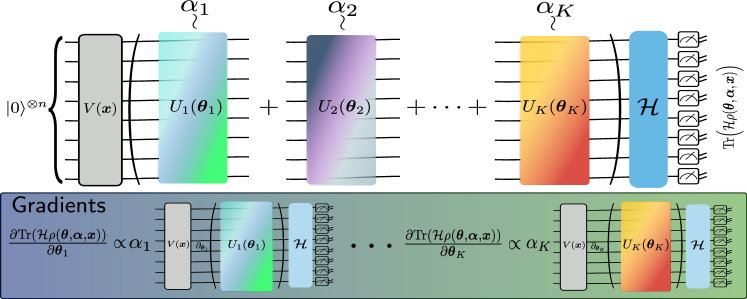
Figure 1: Density quantum neural networks.
The density quantum neural network with $K$ sub-unitaries, $\mathcal{U}=\{U(\boldsymbol{\theta}_{1}),U(\boldsymbol{\theta}_{2}),\dots,U(\boldsymbol{\theta}_{K})\}$. In each instantiation of $\rho$, an index $k\in[1,\dots,K]$ is sampled according to the distribution $\boldsymbol{\alpha}=\{\alpha_{k}\}_{k=1}^{K},\sum_{k}\alpha_{k}=1$. This sub-unitary is applied to the initial state $\ket{\psi(\boldsymbol{x})}=V(\boldsymbol{x})\ket{0}^{\otimes n}$ and measured with the observable $\mathcal{H}$. As a result, the average output from the network is $\text{Tr}\Big{(}\mathcal{H}\rho(\boldsymbol{x},\boldsymbol{\theta})\Big{)}$. In the case where no parameters are shared across the sub-unitaries, the gradients of the full state simply involves computing gradients for each sub-unitary individually.

Modern deep learning owes much of its success to the existence of efficient gradient-based methods to train large and deep neural networks. The backpropagation algorithm [1], and its variants, enable the computation of gradients throughout the entirety of the network, with an overhead not much larger than the evaluation of the network itself. In order to build and train successful models for quantum neural networks in quantum machine learning (QML) problems, we must have training protocols which scale in a similarly efficient fashion to their classical counterparts. Current approaches for evaluating gradients of trainable quantum models such as parameterised quantum circuits (PQCs) [2, 3, 4, 5] (commonly referred to as quantum neural networks (QNNs)) unfortunately do not generally possess such an efficient scaling. If the evaluation of gradients of a QNN requires computation which even scales linearly in the number of parameters, this renders the model effectively untrainable at scale. Unfortunately, such a linear scaling does appear in, for example, the parameter-shift rule for QNNs [6, 7, 8, 9, 10, 11], a popular method which enables the computation of exact (i.e., not relying on approximate finite differences) gradients. For example, applying the parameter-shift rule to a QNN with trainable parameters only located in fixed-axis single-qubit Pauli rotations, requires two individual circuits to run per parameter, leading to a $\mathcal{O}(M)$ gradient scaling for $M$ parameters. As a second example, recent proposals for orthogonal quantum neural networks [12] (OrthoQNNs) contain $\mathcal{O}(n^{2})$ parameters to fully parameterise an orthogonal transformation (i.e. an $n\times n$ orthogonal matrix) on an input vector of size $n$. Using a generalisation of the parameter-shift rule, training such an orthogonal ‘layer’ would require the evaluation of $\sim 40,000$ separate circuits to operate on vectors of length $n=100$. Scaling this to the size of billion or trillion-parameter deep neural networks clearly will not be feasible. Furthermore, in the current NISQ era, access to quantum processing units (QPU) is limited due to the scarcity of devices and the monetary expense of running circuits. Therefore, to properly test proposals for large-scale quantum models, the models need to be as efficient as possible to train.

QNN ansatz	$N_{\textsf{params}}$	$N_{\textsf{grad}}$	$N_{\textsf{params}}$	$N_{\textsf{grad}}$
	Original	Original	This work	This work
$D$ layer hardware efficient  [14]	$\mathcal{O}(nD)$	$\mathcal{O}(nD)$	$\mathcal{O}(nD)$	$\mathcal{O}(D)$
Equivariant XX [15]	$\mathcal{O}(G)$	$\mathcal{O}(1)$	$\mathcal{O}(KG)$	$\mathcal{O}(K)$
HW pres. [12] - pyramid	$\mathcal{O}(n^{2})$	$\mathcal{O}(n^{2})$	$\mathcal{O}(n)$	$\mathcal{O}(1)$
HW pres. [16] - butterfly	$\mathcal{O}(n\log(n))$	$\mathcal{O}(n\log(n))$	$\mathcal{O}(n\log(n))$	$\mathcal{O}(\log(n))$
HW pres. [17] - round-robin	$\mathcal{O}(n^{2})$	$\mathcal{O}(n^{2})$	$\mathcal{O}(n^{2})$	$\mathcal{O}(n)$

Table 1: Summary of gradient scalings for training density quantum neural networks.
Number of gradient circuits ($N_{\textsf{grad}}$) required to estimate full gradient vector for original quantum neural networks versus their density QNN counterparts each with $N_{\textsf{params}}$ parameters acting on $n$ qubits. The equivariant XX ansatz [15], an example of a commuting-generator circuit contains $G$ commuting unitaries ($G$ depends on the maximum locality chosen), $K$ versions of which can be combined to give a density version. We suppress precision factors of $\mathcal{O}(\varepsilon^{-2})$ and $\mathcal{O}(\log(\delta^{-1}))$ which are the same in all cases, assuming a direct sampling method to evaluate gradients.

1.1   The search for quantum backpropagation

To tackle this, some recent works have proposed methods to study whether QML models are even capable of backpropagation-like scaling. To this end, Ref. [13] proved that in general, the answer is, unfortunately, no - there are cases where a backpropagation scaling is impossible based on computational assumptions for quantum models, with certain data input formats. In light of this, one could ask - is a favourable scaling possible when specific structures are introduced to the model or learning algorithm? Indeed, Ref. [13] proved that a backpropagation scaling (in terms of the number of queries) was possible by using multiple copies of the unknown input quantum states. Furthermore, Ref. [15] proposed specific circuit architectures (QNN “ansätze”) which enable efficient gradient computation. These circuits enforce precise commutativity relations between their components, which enables parallel estimation of gradients. The authors found families of circuits whose gradients could be estimated with $\mathcal{O}(1)$ gradient circuit queries - either using a single circuit or with the number of circuits scaling at most with the number of such commuting blocks within a circuit. If it were possible to decompose the OrthoQNNs into $n$ of these blocks, the number of circuits would reduce from $\sim 40,000$ to $\sim 400$ - a significant practical saving. However, such QNN ansätze come with two caveats. First, at the expense of reducing query complexity - the diagonalisation technique necessarily requires the circuit depth to increase (as a diagonalising operation must be appended before the measurement), and hence the physical runtime per circuit is increased. In at least one case, this increased depth does not theoretically cancel the query complexity speedup in gradient estimation, but it is nevertheless an important consideration. The second caveat (noted by the authors) is the potentially limited expressibility of such models, on account of their commuting features.

Here, we attempt to tackle the expressibility/ trainability question by proposing a family of QNN models which include randomisation. Specifically, by attaching a probability distribution to a set of ‘sub-unitaries’, and applying the sub-unitaries to an input state according to said distribution, we can represent the output as a classical mixture of the components in the density matrix formalism of quantum mechanics. We call the resulting model density quantum neural networks (DenQNNs) for brevity. The randomisation means that a single forward pass through the model does not require more time than the more common pure-state QNN model. Furthermore, the resultant model linearity ensures the gradient evaluation and trainability depends on the specific choice of sub-unitaries. If they are chosen to be a commuting-block family, we inherit efficient trainability in the DenQNN framework from the parent family of models, but with increased expressivity. If we tackle the un-trainability of orthogonal quantum neural networks using the density formalism, we can extract a family of efficiently trainable sub-unitaries which have minimal performance loss despite reduced parameter counts, and in some cases even perform better.

The generality of the density framework is very similar to, and in some cases falls under the umbrella of recently proposed post-variational quantum neural networks [18] and also the framework of variational measurement-based quantum computation (MBQC) [19]. We discuss the subtleties of these connections later. Finally, we also discuss the relationship of the DenQNN model to the notion of dropout, a powerful and common ingredient in classical machine learning models. We argue that there are caveats to this comparison, which is usually made offhand in the literature, but we propose at least one method to align the dropout method to the DenQNN framework more closely.

Article structure

This article is structured as follows. In Section 2, we elaborate on some previous work and introduce the concept of backpropagation, the parameter-shift rule and commuting-block and orthogonal circuits. Next, in Section 3, we describe the proposal for adding randomisation and prove the gradient evaluation statements - defining density quantum neural networks. Then, in Section 4, we demonstrate the viability of the density QNN model by testing the model on three example QNN ansätze, the hardware efficient ansatz from Ref. [14], equivariant commuting QNNs from Ref. [15] and Hamming-weight preserving orthogonal neural networks of Ref. [12]. For the latter two examples, we give numerical results on synthetic translationally-invariant data and MNIST digit classification respectively. Finally, we conclude and discuss potential future work in Section 5.

In Table 1 we give a summary of gradient query complexity for the ‘pure state’ QNN models we study in this work, and their counterparts when converted into the density QNN formalism.

Appendix structure

In the appendices, we provide proofs of the parameter-shift rule for orthogonal quantum neural networks (specifically using RBS (App. A.1) and FBS (App. A.2) gates). We give explicit proof of the gradient evaluation for density QNNs in  App. B and some subtleties relating to the measurement and gradient observables required for a backpropagation scaling with orthogonal-inspired density quantum neural networks in App. C. The latter discussion also applies to the original pure state OrthoQNNs. Then, in App. D we discuss the connection between density QNNs and dropout, an important primitive in classical machine learning, and which such density models have been compared to in the quantum literature. Finally, in App. E we discuss the generalisation of density QNNs incorporating data re-uploading and give details of experimental hyperparameter optimisation in F.1.

2   Background

2.1   Backpropagation

There are many methods to compute derivatives in computer programming, some of which have been adopted in the quantum programming world. These include 1) manual calculation, 2) numerical differentiation, 3) symbolic differentiation and 4) automatic or algorithmic differentiation (AD). The two primary operation modes of AD are the forward and reverse modes. The forward mode computes Jacobian-vector products, $\boldsymbol{J}_{\boldsymbol{f}}\boldsymbol{v}$ while reverse computes vector-Jacobian product, $\boldsymbol{v}^{\top}\boldsymbol{J}_{\boldsymbol{f}}$, where $[\boldsymbol{J}_{\boldsymbol{f}}]_{ij}:=\partial\boldsymbol{f}_{i}/\partial\boldsymbol{x}_{j}$ is the Jacobian - the matrix of partial derivatives of $f$ with respect to inputs, $\boldsymbol{x}$. With suitable choices of $\boldsymbol{v}$ (i.e. unit vectors) the forward/reverse modes compute a single column/row of the Jacobian. This apparently subtle difference is actual crucial in practice, as it depends on the input and output dimensions of the function $\boldsymbol{f}:\mathbb{R}^{n}\rightarrow\mathbb{R}^{m}$. Many problems in machine learning where the backpropagation algorithm [1, 21, 22] is applied (reverse mode AD) will have $n\gg m$ (billions of parameters mapping to a small number of classes for example - the Jacobian is extremely wide), which is significantly more efficient than forward mode as we can compute $\partial\boldsymbol{f}_{i}/\partial\boldsymbol{x}_{j}$ for all parameters $j$ simultaneously. However, it does come with the caveat of increased memory to store intermediate gradient computations and is inherently sequential.

In terms of complexity, we can define a ‘backpropagation’ scaling, i.e. the resource scaling which the backpropagation algorithm obeys, and which we ideally would strive for in quantum models. Specifically:

Definition 1 (Backpropagation scaling [13, 15]).

Given a parameterised function, $f(\boldsymbol{\theta}),\boldsymbol{\theta}\in\mathbb{R}^{D}$, with $f^{\prime}(\boldsymbol{\theta})$ being an estimate of the gradient of $f$ with respect to $\boldsymbol{\theta}$ up to some accuracy $\varepsilon$. The total computational cost to estimate $f^{\prime}(\boldsymbol{\theta})$ with backpropagation is bounded with:

$$\mathcal{T}(f^{\prime}(\boldsymbol{\theta}))\leq c_{t}\mathcal{T}(f(\boldsymbol{\theta}))$$ (1)

and

$$\mathcal{M}(f^{\prime}(\boldsymbol{\theta}))\leq c_{m}\mathcal{M}(f(\boldsymbol{\theta}))$$ (2)

where $c_{t},c_{m}=\mathcal{O}(\log(D))$ and $\mathcal{T}(g)/\mathcal{M}(g)$ is the time/amount of memory required to compute $g$.

In plain terms, a model which achieves a backpropagation scaling according to Definition 1, particularly for quantum models, implies that it does not take significantly more effort, (in terms of number of qubits, circuit size, or number of circuits) to compute gradients of the model with respect to all parameters, than it does to evaluate the model itself.

2.2   Quantum neural networks and the parameter-shift rule

Due to the black box nature of quantum circuits, we do not have access easily to intermediate information in the computation, and so we cannot build directly a computational graph as used by AD frameworks. This means, to compute gradients for PQCs, we must rely on other techniques, or clever manipulation of quantum information [13]. Currently, the most well established method (we discuss others later in the text) to compute (analytic) PQC gradients on quantum hardware is via the so-called parameter-shift rule. First hinted at by Ref. [23], and explicitly derived by [6], the rule has been extensively studied and generalised [24]. Starting with a QNN ansatz as follows:

$$\ket{\psi(\boldsymbol{\theta},\boldsymbol{x})}=\mathcal{U}(\boldsymbol{\theta})V(\boldsymbol{x})\ket{0}^{\otimes n}\\ \mathcal{U}(\boldsymbol{\theta})=\prod_{j=1}^{N}U_{j}(\theta_{j})=\prod_{j=1}^{N}e^{i\theta_{j}G_{j}}$$ (3)

Where $\boldsymbol{\theta}:=\{\theta_{1},\dots,\theta_{N}\}$ are trainable parameters, $V(\boldsymbol{x})$ is some initial state preparation unitary acting on an initial state, and $\mathcal{G}=\{G_{j}\}_{j=1}^{N}$ are a set of Hermitian generators. The output of this state is measured to extract expectation values a Hamiltonian, $\mathcal{H}$ (more generally expectations of a set of Hermitian observables, $\{\mathcal{O}_{k}\}$) :

$$\mathcal{L}(\boldsymbol{\theta},\boldsymbol{x})=\bra{\psi(\boldsymbol{\theta},\boldsymbol{x})}\mathcal{H}\ket{\psi(\boldsymbol{\theta},\boldsymbol{x})}\\ =\Tr\left(\mathcal{H}\rho(\boldsymbol{\theta},\boldsymbol{x})\right),\\ \rho(\boldsymbol{\theta},\boldsymbol{x}):=\outerproduct{\psi(\boldsymbol{\theta},\boldsymbol{x})}{\psi(\boldsymbol{\theta},\boldsymbol{x})}$$ (4)

The parameter-shift rule evaluates the gradients of $\mathcal{L}$ with respect to each parameter, $\theta$, by evaluating expectations with respect to some number of ‘shifted’ states/circuits, $\ket{\psi(\boldsymbol{\theta}+\boldsymbol{\beta}_{j},\boldsymbol{x})}$, with $\boldsymbol{\beta}_{j}:=[0,\dots,\underbrace{\beta}_{j},\dots,0]^{\top}=\beta\boldsymbol{e}_{j}\in\mathbb{R}^{N}$. The gradient of $\mathcal{L}$ with respect to a single $\theta_{j}$ is then:

$$\frac{\partial\mathcal{L}}{\partial\theta_{j}}=\sum_{i}^{D}\gamma_{i}\mathcal{L}(\boldsymbol{\theta}+\boldsymbol{\beta}_{j},\boldsymbol{x})$$ (5)

The coefficients $\boldsymbol{\gamma}=\{\gamma_{i}\}_{i=1}^{D}$ depend on the unitary, $U_{j}(\theta_{j})$. If $G_{j}$ has two unique eigenvalues, e.g. $G_{j}\in\{\textsf{X},\textsf{Y},\textsf{Z}\}$ we have $D=2$ and $\boldsymbol{\beta}_{\pm}=\pm\frac{\pi}{2},\boldsymbol{\gamma}_{\pm}=\frac{1}{2}$ for every parameter. Hence, for a QNN with $N$ trainable parameters, we assume a forward pass (single loss evaluation) as a constant time operation, $\mathcal{T}(\textsf{QNN}(\boldsymbol{\theta}))=\mathcal{O}(1)$. However, the gradient requires $\mathcal{O}(N)$ extra ‘shifted’ circuit evaluations so $\mathcal{T}(\textsf{QNN}^{\prime}(\boldsymbol{\theta}))=\mathcal{O}(N)$ (ignoring other parameters). This is similar to the forward AD gradient scaling, but far removed from the efficiency of backpropagation.

There are two notes to make on this point. The first is that the above applies to computing gradients of QNNs/VQAs/PQCs on quantum hardware. When simulating the execution of quantum circuits, we of course can manipulate the computational graph, and hence evaluate gradients. Such schemes are implemented for training quantum circuits in, e.g. Pennylane [25], TensorFlow Quantum [26] or Yao [27] via either naïve or adjoint [28] gradient calculation. Specifically, direct/naïve computation of gradients in circuit simulations is essentially a forward gradient mode, with a corresponding time overhead (as in the parameter-shift rule) while plugging circuit simulation directly into AD frameworks in reverse mode results in a memory overhead. In contrast, the adjoint method achieves a ‘true’ backpropagation scaling on statevector simulators, and in exploiting the reversible nature of quantum operations can also achieve a constant memory overhead. Obviously, though there is the initial exponential memory overhead of simulating statevectors (a forward pass is not efficient).

2.3   Commuting-block quantum neural networks

A proposal to avoid the linear parameter-shift scaling overhead is to design specific circuit structures which admit efficient gradient extraction. To this end, Ref. [15] defined several families of QNNs which achieve this goal. The first family is commuting-generator circuits, for which all the generators in eq. (3) commute with each other, $[G_{i},G_{j}]=0\leavevmode\nobreak\ \forall i,j$. At a high level, given a measurement observable, $\mathcal{H}$, each generator (assuming they mutually commute) defines a gradient observable, $\mathcal{O}_{k}:=[G_{k},\mathcal{H}]$:

$$\frac{\partial\mathcal{L}}{\partial\theta_{k}}=i\bra{\psi(\boldsymbol{\theta},\boldsymbol{x})}[G_{k},\mathcal{H}]\ket{\psi(\boldsymbol{\theta},\boldsymbol{x})}$$ (6)

Further, if all generators commute or anticommute with $\mathcal{H}$, i.e. $[G_{k},\mathcal{H}]=0$ or $\{G_{k},\mathcal{H}\}=0$ for all $k$, one can show that the gradient operators, $\mathcal{O}_{k}$, all mutually commute [15]. As a result, $\mathcal{O}_{k}$ are simultaneously diagonalizable and their statistics can be extracted in parallel, using a single circuit query. In practice, the operators are diagonalized by appending a ‘diagonalizing’ unitary to the end of the original circuit, rotating the gradient measurements into the (for example) computational basis. Measuring this circuit $M$ times and postprocessing gives us the estimates (up to measurement shot noise) of all gradients. One can also extract higher order gradient information (second derivatives etc.) but with a decreasing precision [15].

When specialising these circuits to only generators of tensor product of Pauli operators (‘commuting-Pauli-generator circuits’), the overall gradient circuit has depth $T(n)+\mathcal{O}\big{(}\frac{n}{\log(n)}\big{)}$ where $T(n)$ is the depth of the original QNN on $n$ qubits. For certain families of commuting-Pauli-generator circuits (e.g. those whose generators are supported on a constant number of qubits), the overall depth will be $T(n)$, in line with backpropagation scaling.

These commuting circuits may be limited in expressivity, and may also be efficiently classically simulatabl depeding on the data encoding. To address this, Ref. [15] generalises the above to include blocks of commuting circuits. Here, a single circuit eq. (3) is decomposed into $B$ blocks or layers, so the ansatz has the following form:

$$\mathcal{U}(\boldsymbol{\theta})=\prod_{b=1}^{B}\prod_{j=1}^{N_{b}}U_{b}(\boldsymbol{\theta}^{b}_{j})=\prod_{b=1}^{B}\prod_{j=1}^{N_{b}}e^{i\theta^{b}_{j}G^{b}_{j}}$$ (7)

The blocks are such that the generators of unitaries in different blocks must obey a fixed (but not necessarily commuting) commutation relation. Specifically, they consider the case where generators between different blocks either mutually commute ($[G^{b}_{j},G^{b^{\prime}}_{k}]=0,\forall j,k,b\neq b^{\prime}$), or anti-commute ($\{G^{b}_{j},G^{b^{\prime}}_{k}\}=0$). These commuting-block circuits were shown to have a gradient computation scaling in the number of blocks, $B$, rather than the number of parameters (via Theorem $5$ in Ref. [15]). Since, in many cases $B$ can either be user specified (i.e. a constant), or growing logarithmically in the number of qubits $n$, this renders the number of gradient queries tractable.

2.4   Hamming-weight preserving quantum neural networks

Motivated by the gradient scaling achievable by commuting block circuits, we seek to apply these results to known families of quantum neural networks which admit favourable properties beside gradient scaling, such as interpretability. Specifically, we target orthogonal quantum neural networks defined in several recent works [12, 16, 29]. These QNNs are special cases of Hamming-weight preserving unitaries, or $U(1)$ equivariant circuits [30]. Such circuits can act on states which have a fixed ($k$) Hamming-weight input or on superpositions of different Hamming-weight states. In the former case, the dimension of the Hamming-weight $k$ subspace and its dynamical Lie algebra [31], a concept useful in probing barren plateaus and expressibility in quantum neural networks, is $\binom{n}{k}$ and $\mathcal{O}\left(\binom{n}{k}^{2}\right)$ respectively. As such, these models lack barren plateaus and admit efficient classical simulation if $k$ is small. In the latter, such unitaries can be written in a block diagonal form which each block, $k$, acting independently on the Hamming-weight $k$ subspace [16, 29, 32].

For concreteness in the rest of this work, we focus on the restriction to the Hamming weight $k=1$ subspace. We note however, that this restriction to $k=1$ does not limit the idea or techniques of this work - the methods are equally applicable to generic Hamming-weight preserving quantum neural networks.

Choosing $k=1$ gives so-called orthogonal quantum neural networks (OrthoQNN), which efficiently parameterise orthogonal transformations on input data (encoded in a Hamming-weight $k=1$ initial state). Orthogonality of weight matrices is desirable in classical machine learning, as it directly combats negative features of training such as vanishing or exploding gradients in, for example, temporal or sequential models, such as recurrant neural networks (RNNs). However, orthogonality is an expensive property to enforce - it is not natively guaranteed to propagate using optimisation methods like gradient descent.

The engine of an OrthoQNNs [12] (also see Ref. [33, 17]) are so-called reconfigurable beam splitter (RBS) gates, or Givens’ rotations, which have the following form:

$$\textsf{RBS}(\theta)=e^{-i\frac{\theta}{2}\left(\textsf{Y}\otimes\textsf{X}-\textsf{X}\otimes\textsf{Y}\right)}\\ =\left(\begin{array}[]{cccc}1&0&0&0\\ 0&\cos(\theta)&-\sin(\theta)&0\\ 0&\sin(\theta)&\cos(\theta)&0\\ 0&0&0&1\end{array}\right)$$ (8)

Several ansätze with these operations can be defined, each aimed primarily at differentiating between quantum hardware connectivies, which can be seen in Fig. 2. We have the ‘pyramid’, ‘X’ and ‘butterfly’ ansätze in  Fig. 2 a), b) and c) respectively. These have (in the same order) $n(n-1)/2$, $2n-3$ and $\frac{n}{2}\log(n)$ gates with circuit depths $2n-3$, $n-1$ and $\log(n)$, for an $n$ qubit input. Each of these RBS circuits represents an efficient quantum parameterisation of a (potentially restricted) orthogonal matrix. Specifically, the pyramid layout (Fig. 2a) contains exactly the same number of free parameters as an arbitrary orthogonal matrix with determinant $=1$ ($\mathsf{SO}(n)$) and so one can directly construct a mapping from the RBS parameters in the circuit to the matrix elements. Matrices with determinant $=-1$ can be achieved with an extra Pauli Z operation [12]. One can also generalise OrthoQNNs into compound QNNs, which use fermionic beam splitter (FBS), a generalisation of RBS which we discuss in A.2. These compound QNNs can be represented by compound matrices acting on higher Hamming-weight ($k>1$) or superpositions thereof.

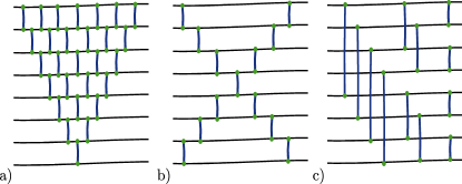
Figure 2: Ansätze for orthogonal quantum neural networks [12, 16]. a) Pyramid circuit, b) X circuit, c) Butterfly circuit. Each gate corresponds to an RBS gate with (potentially different) parameter $\theta$. With respect to the number of qubits, $n$, the depths of each of these layers is $2n-1,n-1$ and $\log(n)$ respectively.

2.5   Post-variational quantum neural networks

The above discussions and models have assumed, as is standard, that the proposed quantum neural network model consists of a single trainable ansatz unitary. In other words, a single component of the loss function (with respect to a particular input), $\Tr\left(\mathcal{O}_{k}\rho(\boldsymbol{\theta},\boldsymbol{x})\right)$ is induced by a single, and fixed, unitary creating the parameterised model $\rho(\boldsymbol{\theta},\boldsymbol{x})$. However, the recent work of Huang and Rebentrost [18] proposed post-variational QNNs (PVQNNs). PVQNNs originated from a proposal to use classical combinations of quantum states to solve, e.g. systems of linear equations [34] and gives more flexibility to single-ansatz QNN models.

The most general proposal of Ref. [18] involves predefining a collection of $K$ sub-unitaries, $\{U_{i}\}_{i=1}^{K}$ and $Q$ observables, $\{\mathcal{O}_{j}\}_{j=1}^{Q}$. Then, in analogue to eq. (4), a single function evaluation is given by:

$$\Tr\left(\mathcal{O}\rho(\boldsymbol{\theta},\boldsymbol{x})\right)\underbrace{\longrightarrow}_{\textsf{PVQNN}}\Tr\left(\mathcal{O}_{k}\rho_{j}(\boldsymbol{x})\right)=:\mathcal{Q}_{kj}\\ \rho_{j}(\boldsymbol{x}):=U_{j}\rho(\boldsymbol{x})U^{\dagger}_{j}$$ (9)

where $\rho(\boldsymbol{x})$ is some (fixed) data-encoded state for the input $\boldsymbol{x}$. The components $\mathcal{Q}_{kj}$ are computed on a quantum computer, and are then linearly combined with parameters $\alpha_{k,j}$ to give the ultimate output of the model: $\mathcal{E}(\boldsymbol{\alpha}):=\sum_{kj}\alpha_{kj}\mathcal{Q}_{kj}$.

In an extreme case, all the unitaries, $U_{j}$, may be absorbed into the observables without losing generality, we can define $\mathcal{O}_{kj}(\boldsymbol{\theta})\leftarrow U_{k}(\boldsymbol{\theta}_{k})\mathcal{O}_{j}U^{\dagger}_{k}(\boldsymbol{\theta}_{k})$. Notice in this formalism that the elements $\mathcal{Q}_{kj}$ are parameter independent, in contrast to the standard model of QNNs where the trainable parameters reside in the unitaries, $U_{k}$. As discussed by [18], the combination of $\mathcal{Q}_{kj}$ with $\alpha_{ij}$ allow the generation of arbitrary quantum transformations on the input state, in which case, $R=K\times Q$ (overall number of $\mathcal{O}_{kj}$’s) should be exponential in the number of qubits in $\rho(\boldsymbol{x})$, $R\leq 4^{n}$. To avoid evaluating an exponential number of quantum circuits, it is clearly necessary to employ heuristic strategies or impose symmetries to choose a sufficiently large or complex pool of operators $\mathcal{O}_{ij}$ and achieve a sufficiently expressive model for $\mathcal{E}(\boldsymbol{\alpha})$. In light of this, Ref [18] proposes an ansatz expansion strategy via ansatz trees [34] or gradient heuristics and an observable construction strategy, the latter proposal having similarities to classical shadows [35, 36] in that a general observable can be constructed via combinations of sufficiently many Pauli strings.

3   Density quantum neural networks

In the previous sections, we introduced the post-variational QNNs of Ref. [18], the orthogonal family of QNNs [12, 37], and the commuting-block QNNs of Ref. [15]. Each of these has their own advantages (which we summarise in Fig. 3):

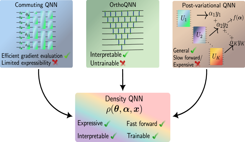
Figure 3: Proposed advantages of density quantum neural networks.
Distilling ingredients from QNN families. The commuting QNNs have efficient gradients but may be of limited expressibility. The OrthoQNNs are interpretable in their data transformations but are difficult to train on quantum hardware. The post-variational QNNs are very general, but a single forward pass requires many circuit evaluations. The DenQNN can increase the expressibility of a trainable circuit, can make an interpretable circuit trainable, and requires no extra overhead than a usual single unitary QNN on a forward pass. We elaborate on this in the main text.

• Post-variational QNNs are arguably one of the most expressive models possible, given their generality.

• Hamming-weight preserving QNNs (OrthoQNNs) have desirable data transformation features.

• Commuting-block QNNs have efficiently extractable gradients.

Let us define density quantum neural networks (DenQNNs) as follows:

We argue that the DenQNN model allows one to take their preferred model, and keep the positive features but yet remove some of its limitations. Specifically, we do this for OrthoQNNs, commuting-block QNNs and PVQNNs as examples.

For this work, we assume data is ‘classical’ and must be explicitly encoded in the quantum system. Most generally, we can measure the state $\rho(\boldsymbol{\theta},\boldsymbol{\alpha},\boldsymbol{x})$ with a collection of observables, $\{\mathcal{O}_{j}\}_{j=1}^{Q}$ as in the PVQNN to produce a vector of outputs given by $[\Tr(\mathcal{O}_{1}\rho(\boldsymbol{\theta},\boldsymbol{\alpha},\boldsymbol{x})),\dots,\Tr(\mathcal{O}_{Q}\rho(\boldsymbol{\theta},\boldsymbol{\alpha},\boldsymbol{x}))]^{\top}$.

In the PVQNN framework, the parameters $\alpha_{k}$ are arbitrary, but here we enforce that they are a (discrete) distribution, hence we have the constraint $\sum_{k}\alpha_{k}=1$. Taking $\boldsymbol{\alpha}:=\{\alpha_{k}\}_{k}$ to be a distribution means that the state eq. (10) can be prepared relatively straightforwardly on a quantum computer via randomisation, but only in a statistical manner. This is in contrast to arbitrary mixed states which in general are difficult to prepare on quantum computers. Specifically, each time we need a realisation of the state eq. (10), we simply sample an index $k$ according to $\alpha_{k}$ and apply the corresponding sub-unitary $U_{k}(\boldsymbol{\theta}_{k})$ to the input state. The DenQNN has then the interpretation of the expected state from the network.

Introducing randomisation to the unitaries in the model is reminiscent of a quantum version of dropout [38, 39] in classical neural networks, as has been remarked in recent works [40]. We argue that, at least in the naïve viewpoint, this is not a correct interpretation for the density QNN framework. We can however make an adaption of the model which more closely aligns to the classical dropout mechanism. We discuss in App. D.1.

Finally, we note that outside of the post-variational framework, using trainable mixed states in variational quantum algorithms is not a new concept in and of itself [41, 42]. in particular, the

However, here we focus on defining density-based models which are compatible with fast gradient estimation and are also very implementable in near-term quantum computers.

3.1   Gradient Scaling

A DenQNN eq. (10) has a set of unitaries $\mathcal{U}:=\{U_{k}(\boldsymbol{\theta}_{k})\}_{k=1}^{K}$. These unitaries could be OrthoQNN unitaries or an entire commuting block unitary of [15]. In the latter case, each unitary, $U(\boldsymbol{\theta}_{i})$, contains $B_{i}$ blocks, each of which could have its own set of parameters. Then, a single parameter in the model is indexed as $\theta^{bj}_{k}$, where $k$ indexes the unitary in the mixture (eq. (10)), $b$ indexes the block, $b\in\{1,\dots B_{k}\}$, and $j$ indexes the parameters within each block, $j\in\{1,\dots N_{B_{k}}\}$.

If the component sub-unitaries in the density model are each efficiently trainable, then the model will be also. ‘Efficiency’ here refers to a backpropagation-like scaling if the sub-unitaries are backpropagation trainable, and a parameter-shift scaling otherwise, which we formalise as follows:

Proposition 1 (Gradient scaling for density quantum neural networks).

Given a density QNN as in eq. (10) composed of $K$ sub-unitaries, $\mathcal{U}=\{U_{k}(\boldsymbol{\theta}_{k})\}$, implemented with distribution, $\boldsymbol{\alpha}=\{\alpha_{k}\}$, an unbiased estimator of the gradients of a loss function, $\mathcal{L}$, defined by a Hermitian observable, $\mathcal{H}$:

$$\mathcal{L}(\boldsymbol{\theta},\boldsymbol{\alpha},\boldsymbol{x})=\Tr\Big(\mathcal{H}\rho(\boldsymbol{\theta},\boldsymbol{\alpha},\boldsymbol{x})\Big{missing})$$ (11)

can be computed by classically post-processing $\sum_{l=1}^{K}\sum_{k=1}^{K}T_{\ell k}$ circuits, where $T_{\ell k}$ is the number of circuits required to compute the gradient of sub-unitary $k$, $U(\boldsymbol{\theta}_{k})$ with respect to the parameters in sub-unitary $\ell$, $\boldsymbol{\theta}_{\ell}$. Furthermore, these parameters can also be shared across the unitaries, $\boldsymbol{\theta}_{k}=\boldsymbol{\theta}_{k^{\prime}}$ for some $k,k^{\prime}$.

The proof is given in App. B.1, but it follows simply from the linearity of the model. Now, there are two sub-cases one can consider. First, if all parameters between sub-unitaries are independent, $\boldsymbol{\theta}_{k}\neq\boldsymbol{\theta}_{\ell},\leavevmode\nobreak\ \forall k,\ell$. This gives the following corollary, also in App. B.1.

Corollary 1.

Given a density QNN as in eq. (10) composed of $K$ sub-unitaries, $\mathcal{U}=\{U_{k}(\boldsymbol{\theta}_{k})\}$ where the parameters of sub-unitaries are independent, $\boldsymbol{\theta}_{k}\neq\boldsymbol{\theta}_{\ell},\forall k,\ell$ an unbiased estimator of the gradients of a loss function, $\mathcal{L}$, eq. (11) can be computed by classically post-processing $\sum_{k=1}^{K}T_{k}$ circuits, where $T_{k}$ is the number of circuits required to compute the gradient of sub-unitary $k$, $U(\boldsymbol{\theta}_{k})$ with respect to the parameters, $\boldsymbol{\theta}_{k}$.

The second case is where some (or all) parameters are shared across the sub-unitaries. Taking the extreme example, $\theta_{l}^{j}=\theta_{k}^{j}=:\theta^{j}\leavevmode\nobreak\ \forall k,l$ - i.e. all sub-unitaries from eq. (10) have the same number of parameters, which are all identical. In this case, for each sub-unitary, $l$, we must evaluate all $K$ terms in the sum so at most the number of circuits will increase by a factor of $K^{2}$ - we need to compute every term in eq. (24).

In the case of independent parameters per sub-unitary in eq. (10), one might ask - what are the training dynamics of a model whose gradient for subsections of parameters are completely independent? The first comment is that the model clearly reduces to the usual unitary QNN model for $K=1$, where we have $\alpha_{1}=1$ and

$$\mathcal{L}(\boldsymbol{\theta},\boldsymbol{x})=\Tr\Big(\mathcal{H}\rho(\boldsymbol{\theta},\boldsymbol{x})\Big{missing})\\ =\Tr\Big(\mathcal{H}U_{1}(\boldsymbol{\theta}_{1})\outerproduct{\boldsymbol{x}}{\boldsymbol{x}}U^{\dagger}_{1}(\boldsymbol{\theta}_{1})\Big{missing})\\ =\Tr\Big(\bra{\boldsymbol{x}}U^{\dagger}_{1}(\boldsymbol{\theta}_{1})\mathcal{H}U_{1}(\boldsymbol{\theta}_{1})\ket{\boldsymbol{x}}\Big{missing})\\ =\bra{\psi(\boldsymbol{\theta},\boldsymbol{x})}\mathcal{H}\ket{\psi(\boldsymbol{\theta},\boldsymbol{x})}$$ (12)

so it is at least as expressive as each underlying sub-unitary individually.

Secondly, we have an (potentially) analogous situation classically. Taking a very simple linear layer in a neural network without the activation, $f(W,\boldsymbol{b})=W\boldsymbol{x}+\boldsymbol{b}$. The gradients with respect to the parameters, $W,\boldsymbol{b}$, are independent of each other, $\partial_{W}f=\boldsymbol{x},\partial_{\boldsymbol{b}}f=\mathds{1}$, as in the above. However, this no longer is the case when adding an activation: $f(W,\boldsymbol{b})=\sigma(W\boldsymbol{x}+\boldsymbol{b})$: $\partial_{W}f=\partial_{W\boldsymbol{x}+\boldsymbol{b}}(\sigma(W\boldsymbol{x}+\boldsymbol{b}))\times\boldsymbol{x}$ and $\partial_{\boldsymbol{b}}f=\partial_{W\boldsymbol{x}+\boldsymbol{b}}(\sigma(W\boldsymbol{x}+\boldsymbol{b}))\times\mathds{1}$, where (depending on the activation) the non-differentiated parameters still propagate into the gradients of the differentiated ones.

A final comment to make is that the loss function in eq. (11) assumes only a single datapoint, $\ket{\boldsymbol{x}}$ is evaluated. We can also take expectations of this loss with respect to the training data,

$$\mathcal{L}(\boldsymbol{\theta},\boldsymbol{\alpha})=\underset{\boldsymbol{x}}{\mathbb{E}}\Big{[}\Tr\Big(\mathcal{H}\rho(\boldsymbol{\theta},\boldsymbol{\alpha},\boldsymbol{x})\Big{missing})\Big{]}\\ \approx\sum_{i=1}^{M}\delta_{i}\Tr\Big(\mathcal{H}\rho(\boldsymbol{\theta},\boldsymbol{\alpha},\boldsymbol{x}_{i})\Big{missing})\\ =\sum_{k=1}^{K}\sum_{i=1}^{M}\alpha_{k}\delta_{i}\Tr\Big(\mathcal{H}U_{k}(\boldsymbol{\theta}_{k})\outerproduct{\boldsymbol{x}_{i}}{\boldsymbol{x}_{i}}U^{\dagger}_{k}(\boldsymbol{\theta}_{k})\Big{missing})$$ (13)

for $M$ data samples. Therefore, we increase the number of circuits we must run by a factor of $M$, each of which will have a gradient cost of $\sum_{l=1}^{K}\sum_{k=1}^{K}T_{\ell k}$. One can view eq. (13) as creating an ‘average’ data state $\sum_{i=1}^{M}\delta_{i}\outerproduct{\boldsymbol{x}_{i}}{\boldsymbol{x}_{i}}$, where $\{\delta_{i}\}$ is the empirical distribution over the data and then applying the density sub-unitaries with their corresponding distribution, $\{\alpha_{k}\}_{k}$, or by estimating the elements of the stochastic $K\times M$ matrix with elements $\Tr\Big(\mathcal{H}U_{k}(\boldsymbol{\theta}_{k})\outerproduct{\boldsymbol{x}_{i}}{\boldsymbol{x}_{i}}U^{\dagger}_{k}(\boldsymbol{\theta}_{k})\Big{missing})$. In reality, we also will estimate the trace term in eq. (13) with $S$ measurements shots from the circuit. Incorporating this with the above density model and its gradients, one could also define an extreme gradient descent optimiser in the spirit of [10], sampling over datapoints, measurement shots, measurement observable terms, parameter-shift terms and in our case, sub-unitaries to estimate the loss function and its gradients in a single circuit run.

Now, using the above we can generalise the results of Ref. [15] as follows:

Corollary 2 (Gradient scaling for density commuting-block quantum neural networks).

Given a density QNN on $n$ qubits with a commuting-block structure for each sub-unitary, $k$, where each $k$ has $B_{k}$ blocks within. Assume each sub-unitary has different parameters, $\boldsymbol{\theta}_{k}\neq\boldsymbol{\theta}_{\ell}\leavevmode\nobreak\ ,\forall k,\ell$. Then an unbiased estimate of the gradient can be estimated by classical post-processing $\mathcal{O}(2\sum_{k}B_{k}-K)$ circuits on $n+1$ qubits.

Proof.

This follows immediately from Theorem 1 and Theorem 5. from Ref. [15]. Here, the gradients of a single $B$-block commuting block circuit can be computed by post-processing $2B-1$ circuits, where $2$ circuits are required per block, with the exception of the final block, which can be treated as a commuting generator circuit and evaluated with a single circuit. ∎

Note that this is the number of circuits required, not the overall sample complexity of the estimate. For example, take the single layer commuting-block circuit (just a commuting-generator circuit) with $M$ mutually commuting generators, and a suitable measurement observable, $\mathcal{H}$, such that the resulting gradient observables, $\{\mathcal{O}_{k}|\mathcal{O}_{k}:=[G_{k},\mathcal{H}]\}_{k=1}^{M}$, can be simultaneously diagonalized. To estimate these $M$ gradient observables each to a precision $\varepsilon$ (meaning outputting an estimate $\tilde{o}_{k}$ such that $|\tilde{o}_{k}-\bra{\psi}\mathcal{O}_{k}\ket{\psi}|\leq\varepsilon$ with confidence $1-\delta$) requires $\mathcal{O}\left(\varepsilon^{-2}\log\left(\frac{M}{\delta}\right)\right)$ copies of $\psi$ (or equivalently calls to a unitary preparing $\psi$). It is also possible to incorporate strategies such as shadow tomography [36], amplitude estimation [43] or quantum gradient algorithms [44] to improve the $M$, $\delta$ or $\varepsilon$ parameter scalings for more general scenarios, though inevitably at the cost of scaling in the others.

Now, we began this section by claiming that DenQNN’s inherit favourable properties of their parent models. We begin this with a comparison between density QNNs and post-variational QNNs, and we discuss the other two models in the following sections. PVQNN’s consider the parameters, $\boldsymbol{\alpha}$ to be arbitrary (predicted by a neural network or found as the optimal solution to a convex optimisation problem). This means there is no easy mapping between the data encoded states and the output ‘channel’ $\mathcal{E}(\boldsymbol{\alpha})$ directly on a quantum computer.

By enforcing the distributional requirement on $\boldsymbol{\alpha}$, over the sub-unitaries, $\{U_{k}(\boldsymbol{\theta}_{k})\}$, in the DenQNN model, a single forward pass does not require all $R=P\times Q$ observables $\mathcal{O}_{kj}$ to be evaluated as in the PVQNN framework. Instead given $Q$ observables $\{\mathcal{O}_{j}\}_{j=1}^{Q}$, we only need $R=Q$ circuits to run a forward pass. The effective state, $\rho$, will only exist on average via probabilistic application of the $K$ sub-unitaries. If the observables commute we only require $R=1$ circuit. As such, for the large number of circuits and observables which may need to be implemented to gain sufficiently expressive models, we could gain a significant practical cost saving.

4   Examples

4.1   Hardware efficient quantum neural networks

Let us begin with a toy example (shown in Fig. 4) - the common but much maligned hardware efficient  [14] quantum neural network. These ‘problem-independent’ ansätze were proposed to keep quantum learning models as close as possible to the restrictions of physical quantum computers, by enforcing specific qubit connectivities and avoiding injecting trainable parameters into complex transformations. These circuits are extremely flexible, but this comes at the cost of being vulnerable to barren plateaus [45] and generally difficult to train.

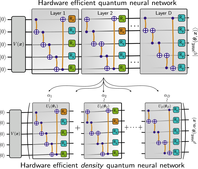
Figure 4: Decomposing a hardware efficient ansatz for a density QNN.
$D$ layers of a hardware efficient (HWE) ansatz with entanglement generated by CNOT ladders and trainable parameters in single qubits $\textsf{R}_{x},\textsf{R}_{y},\textsf{R}_{z}$ gates. $D$ layers extracted into $D$ sub-unitaries with probabilities, $\{\alpha_{d}\}_{d=1}^{D}$ for a density QNN version. Applying the commuting-generator framework to the density version, $\rho^{\mathsf{HWE}}(\boldsymbol{\theta},\boldsymbol{\alpha},\boldsymbol{x})$, enables parallel gradient evaluation in $2D$ circuits versus $2nD$ as required by the pure state version, $\ket{\psi^{\mathsf{HWE}}(\boldsymbol{\theta},\boldsymbol{\alpha},\boldsymbol{x})}$. CNOT direction reversed in subsequent layers to increase sub-circuit differentiation and partially accounting for low circuit depth.

A $D$ layer hardware efficient ansatz on $n$ qubits is usually defined to have $1$ parameter per qubit (located in a single qubit Pauli rotation) per layer. The parameter shift rule with such a model would require $2nD$ individual circuits to run, each for $M$ measurements shots. Given such a circuit, we can construct a density version with $D$ sub-unitaries and reduce the gradient requirements from $2nD$ to $2D$ as the gradients for the single qubit unitaries in each sub-unitary can be evaluated in parallel, using the commuting-generator toolkit. This example is relatively trivial as the resulting unitaries are shallow depth and training each corresponds only to learning a restricted single qubit measurement basis, though it does demonstrate the flexibility of the density framework. In the  Fig. 4, we take a variation of the common CNOT-ladder layout - entanglement is generated in each layer by nearest-neighbour CNOT gates. An initial data encoding unitary, $V(\boldsymbol{x})$, is used to prepare the initial state. Typically, an identical structure is used in each layer, however in the figure we allow each sub-unitary extracted from each layer to have a varying CNOT control-target directionality and different single qubit rotations in each layer. This is to reduce the triviality when moving to a density version - otherwise each sub-unitary would be identical.

4.2   Equivariant quantum neural networks

The above example showed how the density/post-variational formalism allows one to take a circuit which is difficult to train at scale into a variation which is efficiently trainable. In this section, we take the other extreme for a second example. Starting from a circuit which is trainable with backpropagation scaling, we show that the density formalism gives a more expressive model, with minimal loss in training speed.

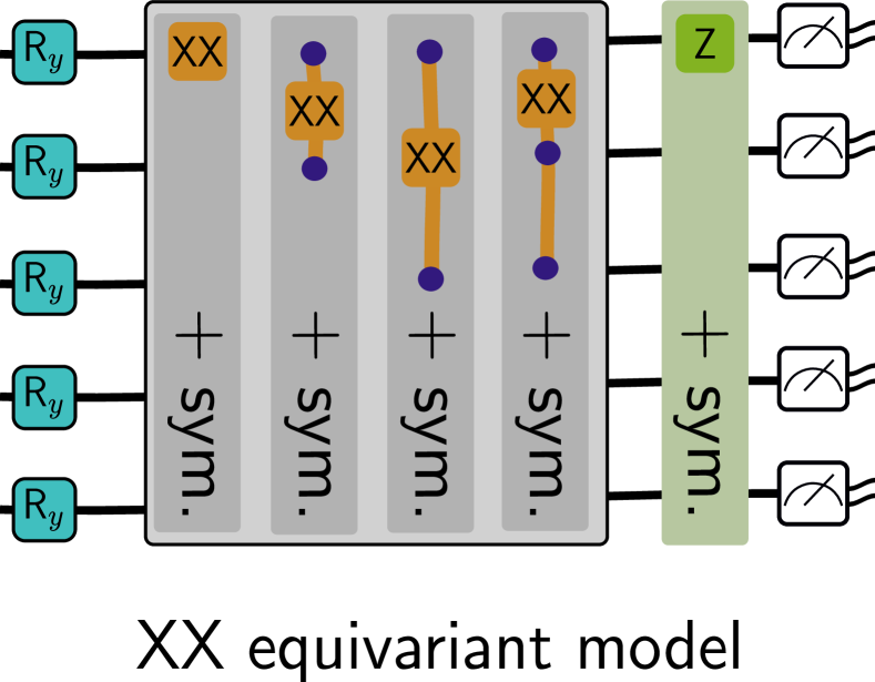
i

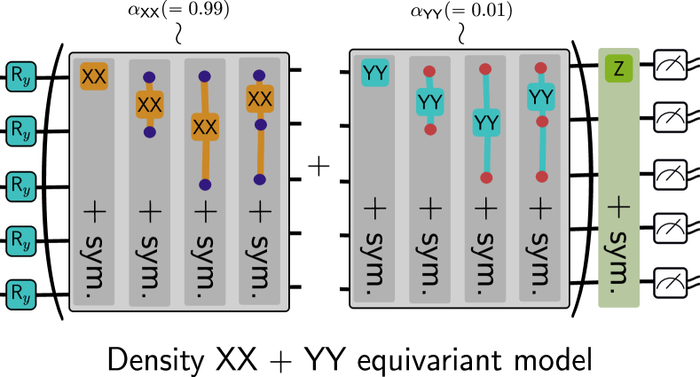
ii

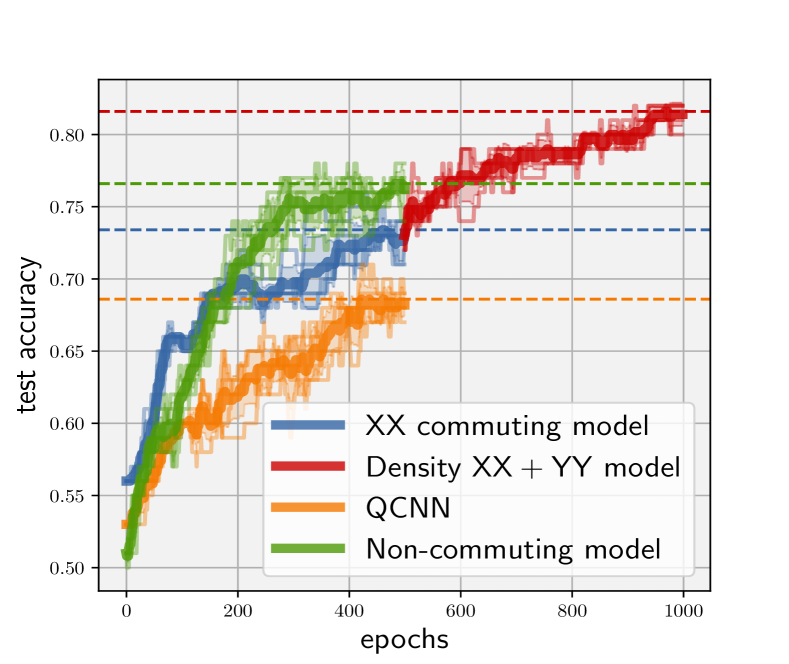
iii

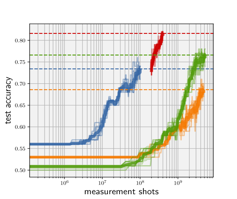
iv

Figure 5: Equivariant density QNN & numerics on noisy bars and dots dataset.
Comparing the performance of the i) commuting-generator XX model with the ii) density QNN with XX + YY sub-unitaries. The former contains up to three-body Pauli-X generated operations with twirling applied to enforce equivariance. The latter contains the same operations as i), but applied with probability $\alpha_{\textsf{XX}}$, along with a second circuit generated by twirled Pauli-Y operations with probability $\alpha_{\textsf{YY}}$. Individually, both sub-circuits in ii) are commuting-generator circuits, so each has efficiently extractable gradients. We also compare against the two other models considered in Ref. [15], the ‘non-commuting’ QNN and the quantum convolutional neural network [46], all on $10$ qubits. The DenQNN is initialised from (separately) pretrained XX and YY commuting models for $500$ epochs, and training continues for another $500$. The lighter lines are $5$ individual training trials, starting from the same initial parameters, with the mean and standard deviation shown in thick lines and the shaded region respectively. We compare test accuracy vs. iii) training epochs and iv) number of overall shots. The performance of all base models saturates by $500$ epochs, but the DenQNN continues improving in performance when initialised by the trained XX model. The gap between the XX model and DenQNN $\textsf{XX}+\textsf{YY}$ in Fig. 5iv is to account for the extra measurement overhead to initialise the YY part of the model, which is trained in parallel with the XX model for $500$ epochs. The DenQNN outperforms all other models, with fewer shots than the QCNN and non-commuting model.

Specifically, we reuse the example from Ref. [15], which is a simplified classification problem. Here, the challenge is classifying bars vs. dots, in a noisy setting. Each datapoint is a $d$-dimensional vector (bar or dot) with either alternating $+1$ and $-1$ values (dot) or sequential periods of $+1$ or $-1$ of length $\lfloor\frac{d}{2}\rfloor$ (bar). Gaussian noise with mean $=0$ and variance $\sigma^{2}$ is added to each vector. In Ref. [15], the translation invariance of the data enables the application of a commuting-generator equivariant ansatz, where each generator consists of a symmetrised Pauli-X string containing up to $K$-body terms. The measurement observable is also a symmeterised Pauli Z string with $K=1$, meaning $\mathcal{H}=\sum_{i=1}^{d}\textsf{Z}_{i}$. Each bar/dot, $\boldsymbol{x}:=[x_{1},\dots,x_{d}]^{\top}\in\mathbb{R}^{d}$, is encode as a Pauli Y rotation per qubit, $x_{i}\mapsto\textsf{R}_{y}(\frac{\pi x_{i}}{2})\ket{0}=\cos(\frac{\pi x_{i}}{4})\ket{0}+\sin(\frac{\pi x_{i}}{4})\ket{1}=:\ket{\boldsymbol{x}}^{ry}_{i}$. This angle-encoding uses the same number of qubits as the unary amplitude encoding in the OrthoQNN above.

Here, we take the original XX ansatz (denoted $U_{\textsf{XX}}(\boldsymbol{\theta})$, see Fig. 5i) and compare against the density model with two sub-unitaries, $\{U_{1},U_{2}\}$. Specifically, we define two sub-unitaries $U_{1}:=U_{\textsf{XX}}(\boldsymbol{\theta})$, weighted by $\alpha_{1}$, and $U_{2}:=U_{\textsf{YY}}(\boldsymbol{\theta})$, weighted by $\alpha_{2}$. The second sub-unitary, $U_{\textsf{YY}}(\boldsymbol{\theta})$, has the exact same structure as $U_{\textsf{XX}}(\boldsymbol{\theta})$, but with the XX generators replaced by Pauli Y generators. The output state is then:

$$f(\boldsymbol{\theta},\boldsymbol{\alpha},\boldsymbol{x},\boldsymbol{\alpha}):=\sum_{i=1}^{d}\sum_{k=1}^{K}\Tr(\textsf{Z}_{i}\rho(\boldsymbol{\theta},\boldsymbol{\alpha},\boldsymbol{x}))\\ \rho(\boldsymbol{\theta},\boldsymbol{\alpha},\boldsymbol{x})=\alpha_{1}U_{\textsf{XX}}(\boldsymbol{\theta})\Big{[}\bigotimes_{j=1}^{d}\ket{\boldsymbol{x}}\bra{\boldsymbol{x}}^{ry}_{j}\Big{]}U^{\dagger}_{\textsf{XX}}(\boldsymbol{\theta})+\\ \alpha_{2}U_{\textsf{YY}}(\boldsymbol{\theta})\Big{[}\bigotimes_{j=1}^{d}\ket{\boldsymbol{x}}\bra{\boldsymbol{x}}^{ry}_{j}\Big{]}U^{\dagger}_{\textsf{YY}}(\boldsymbol{\theta})$$ (14)

Each generator that appears in $U_{\textsf{XX}/\textsf{YY}}(\boldsymbol{\theta})$ is of the form $\textsf{sym}(\textsf{X}_{1})$ or $\textsf{sym}(\textsf{X}_{1}\dots\textsf{X}_{k})$ for some $k\leq K$. The operation sym is the twirling operation used to generate equivariant quantum circuits (in this case, equivariance with respect to translation symmetry). Explicitly:

$$\textsf{sym}(\textsf{X}_{1}) =\textsf{X}_{1}+\textsf{sym}=\sum\nolimits_{i=1}^{d}\textsf{X}_{i}$$

$$\textsf{sym}(\textsf{X}_{1}\textsf{X}_{2}) =\textsf{X}_{1}\textsf{X}_{2}+\textsf{X}_{2}\textsf{X}_{3}+\textsf{X}_{3}\textsf{X}_{4}+\dots+\textsf{X}_{d}\textsf{X}_{1}$$

$$\textsf{sym}(\textsf{X}_{1}\textsf{X}_{3}) =\textsf{X}_{1}\textsf{X}_{3}+\textsf{X}_{2}\textsf{X}_{4}+\dots+\textsf{X}_{d-1}\textsf{X}_{1}$$

$$\textsf{sym}(\textsf{X}_{1}\textsf{X}_{2}\textsf{X}_{3}) =\textsf{X}_{1}\textsf{X}_{2}\textsf{X}_{3}+\dots+\textsf{X}_{d-1}\textsf{X}_{d}\textsf{X}_{1}+\textsf{X}_{d}\textsf{X}_{1}\textsf{X}_{2}$$

In other words, $\textsf{sym}(\textsf{X}_{1}\textsf{X}_{2})$ is a sum of all pairs of X operators on the state with no intermediate trivial qubit, $\textsf{sym}(\textsf{X}_{1}\textsf{X}_{3})$ is a sum of all pairs on the state separated by exactly one trivial qubit (in either direction, visualising the qubits as a $1\textnormal{D}$ chain with close boundary conditions) and so on. We have the exact same pattern in $U_{\textsf{YY}}(\boldsymbol{\theta})$ but replacing every Pauli X generator with a Pauli Y. However, note that in this case since the YY ansatz is in the same basis as the data encoding ($\textsf{R}_{y}$), we have classical simulatability for computing expectation values since the initial circuit is effectively Clifford [15]. The density circuits are visualised in Fig. 5ii which we adapt from [15].

The results of the experiment can be seen in Fig. 5iii and Fig. 5iv. We use the noisy bars and dots dataset as in Ref. [15], for $10$ qubits. We increase the noise to $\sigma=1.8$ to increase the problem difficult. We train the model with train and test data of sizes of $1000,100$ respectively and a batch size of $20$. We use the Adam optimiser with a learning rate of $0.001$ in all cases. We initialise the weighting parameters, $\{\alpha_{1},\alpha_{2}\}=\{\alpha_{\textsf{XX}},\alpha_{\textsf{YY}}\}=\{0.99,0.01\}$ to bias the model towards the (pre-trained) equivariant XX model, and $\boldsymbol{\alpha}$ are also trainable. The formulae to compute the number of shots required by each model (commuting XX, non-commuting, QCNN) is given in Ref. [15]. The number of shots for the DenQNN $\textsf{XX}+\textsf{YY}$ model being $2N_{\textsf{XX}}+2N_{\textsf{YY}}$ where $N_{\textsf{XX}/\textsf{YY}}$ is the number of shots to train the XX, YY models separately (over $500$ epochs for each model). We adapt the code of [47] to generate the results for the commuting, non-commuting and QCNN models.

4.3   Orthogonal quantum neural networks

In the above, we have constructed density QNNs from the hardware efficient ansatz and a translationally equivariant ansatz. For the former, we could reduce the required number of circuits needed to train the model, and for the latter we could improve the performance of the model without a substantial increase the number of gradient circuits.

For our final example(s), we turn to the Hamming-weight preserving quantum neural network ($U(1)$ equivariant), and specifially the orthogonal quantum neural networks (OrthoQNN). As discussed in Section 2.4, these models have desirable properties from a machine learning point of view - they are interpretable and can stabilise training. Again, we stress the below is applicable to compound QNNs A.2 and general Hamming-weight preserving unitaries).

This final example will highlight some features and limitations of the density QNN framework. We begin with a simple density model using only two sub-unitaries $\{U_{1},U_{2}\}$ which are vivisected from a pyramid circuit 2a). However, these sub-unitaries will turn out to be relatively limited, but the constant number of sub-unitaries gives the greatest gradient scaling advantage. To increase the expressive power of the orthogonal density model, we then decompose the butterfly 2c) ansatz, which can decompose into $K=\mathcal{O}(\log(n))$ non-trivial sub-unitaries. This version admits a quadratic to logarithmic reduction in the number of gradient scaling. Finally, in the most complex version, a round-robin ansatz which decomposes into $K=\mathcal{O}(n)$ sub-unitaries, and admits the most modest gradient circuit reduction - only from quadratic to linear. Finally, we allow the model to have data-dependent weightings, $\boldsymbol{\alpha}\rightarrow\boldsymbol{\alpha}(\boldsymbol{x})$, where the distribution is predicted by a (classical) neural network. We show that a round-robin density QNN can outperform the standard pyramid ansatz, while being asymptotically faster to train.

Finally, we discuss the measurement protocol required for the above models to achieve these scalings.

4.3.1   Odd-even pyramid decomposition

We begin with the simplest example which has the greatest gradient query speedup. Given the pyramid circuit Fig. 2a), we create a density QNN, by decomposing the layer into two sub-unitaries, $U_{1}:=U^{\textsf{even}}$ and $U_{2}:=U^{\textsf{odd}}$ which we define as $U_{1},U_{2}$ in eq. (10) respectively.

Now, $U^{\textsf{even}}$ contains the circuit moments where each gate within has an even-numbered qubit as its first qubit (the ‘control’) and $U^{\textsf{odd}}$ contains odd qubit-controlled gates only. The resulting DenQNN state is then (initialised with a uniform distribution weighting, $\boldsymbol{\alpha}$ - but these are also trainable parameters):

$$\rho(\boldsymbol{\theta},\boldsymbol{\alpha}=\left\{\frac{1}{2},\frac{1}{2}\right\},\boldsymbol{x})=\\ \frac{1}{2}\left(U^{\textsf{even}}(\boldsymbol{\theta})\outerproduct{\boldsymbol{x}}{\boldsymbol{x}}U^{\textsf{even}}(\boldsymbol{\theta})^{\dagger}\right)\\ +\frac{1}{2}\left(U^{\textsf{odd}}(\boldsymbol{\theta})\outerproduct{\boldsymbol{x}}{\boldsymbol{x}}U^{\textsf{odd}}(\boldsymbol{\theta})^{\dagger}\right)$$ (15)

All gates in $U_{1}$ and $U_{2}$ mutually commute with each other. and the input state, $\ket{\boldsymbol{x}}=\sum_{j}x_{j}\ket{\boldsymbol{e}_{j}}$, is a unary amplitude encoding of the vector $\boldsymbol{x}$. since the OrthoQNN unitaries are Hamming-weight preserving, the output states, $\ket{\boldsymbol{y}^{\textsf{odd}}},\ket{\boldsymbol{y}^{\textsf{even}}}$ from each sub-unitary are of the form $\ket{\boldsymbol{y}}=\sum_{j}y_{j}\ket{\boldsymbol{e}_{j}}$ for some vector $\boldsymbol{y}$. The typical output of such an OrthoQNN layer is the vector $\boldsymbol{y}$ itself, for further processing in a deep learning pipeline. For our purposes in gradient-based training, due to the linearity and the purity of the individual output states, $\ket{\boldsymbol{y}^{\textsf{even}/\textsf{odd}}}$, we can deal with both individually and classically combine the results.

Now, let us compare the density pyramid QNN to the vanilla pyramid OrthoQNN using the common machine learning benchmark: handwritten MNIST digits. First, we note that density model is no longer strictly an ‘orthogonal quantum neural network’, as orthogonality is no longer preserved by the density layer.

The output of a (pyramid) OrthoQNN is a vector, $\boldsymbol{y}$, which is simply a rotated version of the input feature vector, $\boldsymbol{x}$:

$$\boldsymbol{y}=O^{U}\boldsymbol{x}$$ (16)

for some orthogonal matrix $O^{U}$, generated by the angles of an RBS gates in a Hamming weight preserving unitary, $U$. On the other hand the density output (for two sub-unitaries) is:

$$\boldsymbol{y}=\alpha_{1}\boldsymbol{y}_{1}+\alpha_{2}\boldsymbol{y}_{2}=\alpha_{1}O^{U_{1}}_{1}\boldsymbol{x}+\alpha_{2}O^{U_{2}}_{2}\boldsymbol{x}$$ (17)

where each $\boldsymbol{y}_{k}$ is simply $\boldsymbol{x}$ with a subset of elements rotated by a restricted orthogonal matrix, $O^{U_{k}}_{k}$. The density version therefore outputs a probabilistic linear combination of partially rotated feature vectors. Nevertheless, let us test the two models on real data.

To begin, in order to mitigate biases from unsuitable data encodings or post-processing for either model, we attach a single linear classical neural layer to both the input and output of the model. This allows both models to learn suitable feature vectors and final ‘activation’ functions, which will not necessarily be the same. This enables a more fair comparison with the true capacity of the density QNN which could otherwise be negatively impacted by poor classical processing choices. For completeness, we also remove this (potentially powerful) classical processing layers later. To test the models, we classically simulate them using pytorch and incorporate them into the automatic differentiation framework therein. We stress that in reality, one would require the gradient rules above to train these models on quantum hardware.

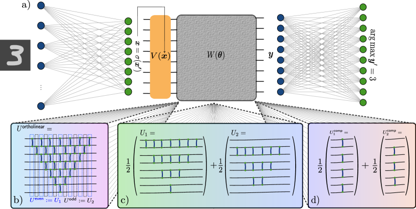
i

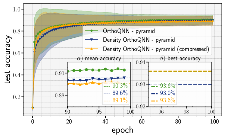
ii

Figure 6: Pure state Hamming-weight preserving (orthogonal) QNN with a pyramid ansatz, and the density QNNs derived from it. 6i) The full models used for numerical results. MNIST data is flattened with a $784\times 8$ linear layer outputting, $\boldsymbol{x^{\prime}}$. A ReLU activation gives $\boldsymbol{x}:=\sigma(\boldsymbol{x^{\prime}}):=\mathsf{ReLU}(\boldsymbol{x^{\prime}})$. A parallel vector loader, $V(\boldsymbol{x})$, is used to encode $\boldsymbol{x}$ in a unary amplitude encoding (suitably normalised), $\ket{\boldsymbol{x}}\propto\sum_{j}x_{j}\ket{\boldsymbol{e}_{j}},\boldsymbol{e}_{j}:=0\cdots 1_{j}\cdots 0$. This is then processed by the quantum operation $W$ with parameters $\boldsymbol{\theta}$, and an outcome vector, $\boldsymbol{y}$, is extracted, and postprocessed into $10$ label classes (digits $\ell\in\{0,1,\dots,9\}$) via a $8\times 10$ linear layer and a softmax function. 6ii) shows the comparison between three models, ‘OrthoQNN - pyramid’, ‘Density OrthoQNN - pyramid’ and ‘Density OrthoQNN - pyramid (compressed)’ which correspond to replacing the $W$ operation by Fig. 6i a), b) or c) respectively. The y-axis shows the test accuracy over all the $10,000$ MNIST test images. The main plot shows the mean (solid line) and standard deviation (shaded region) over the best fraction out of $32$ overall hyperparameter optimisation runs for all three models using optuna. We define ‘best’ to be those runs which achieve $>70\%$ test accuracy, and we give more details in F.1. Insets show the mean ($\alpha$), and best ($\beta$) test accuracies over all hyperparameters in the last $10$ epochs.

We take $60,000$ train and $10,000$ test images from the MNIST dataset. The first linear layer is of size $784\times 8$ to process the $28\times 28$ images to an $8$-qubit feature vector, with a ReLU activation function to produce the circuit input $\boldsymbol{x}$ (Fig. 6i) We then either apply the ortholinear layer $U^{\textsf{ortholinear}}$, or construct the density matrix $\rho(\boldsymbol{\theta},\boldsymbol{\alpha},\boldsymbol{x})=\frac{1}{2}U_{1}(\boldsymbol{\theta}_{1})\outerproduct{\boldsymbol{x}}{\boldsymbol{x}}U_{1}(\boldsymbol{\theta}_{1})+\frac{1}{2}U_{2}(\boldsymbol{\theta}_{2})\outerproduct{\boldsymbol{x}}{\boldsymbol{x}}U_{2}(\boldsymbol{\theta}_{2})$ classically, where $\ket{\boldsymbol{x}}$ is the data-loaded feature vector using the unitary $V(\boldsymbol{x})$. There are various choices one could make to create the unary state, $\ket{\boldsymbol{x}}$, for all the following we assume a parallel vector loader [48, 16] but the choice of loader will depend on the available quanutm hardware.

Again we reiterate that, on quantum hardware, one would not physically prepare the mixed state $\rho(\boldsymbol{\theta},\boldsymbol{\alpha},\boldsymbol{x})$, instead it would only exist on average, by probabilistically applying $U_{1}$ and $U_{2}$ (unless using the dropout interpretation in inference mode as discussed in App. D).

Now, examining Fig. 6ib), one can observe that since many of the gates in both $U_{1}$ and $U_{2}$ are commuting RBS gates acting on the same qubits, we circuit compression is possible into circuits with only a single moment (depth $=1$), as illustrated in Fig. 6ic). Indeed, this is the case - however, we find that even though the two states $\rho(\boldsymbol{\theta},\boldsymbol{\alpha},\boldsymbol{x})$ and $\rho^{\textsf{compressed}}(\boldsymbol{\theta},\boldsymbol{\alpha},\boldsymbol{x})$ are formally equivalent (and actually have identical gradients as will be discussed below), the performance of both variations can be different. From Fig. 6ii, we see the uncompressed version performs better on average over different hyperparameter regimes. However, the compressed version is capable of matching the vanilla pyramid OrthoQNN, when finding the best performing model (the highest test accuracy achieved over all hyperparameters. Nevertheless, both compressed and uncompressed versions benefit from a $\mathcal{O}(n^{2})$ (pyramid OrthoQNN) to $\mathcal{O}(1)$ (density even-odd extraction) gradient scaling advantage since we only have $K=2$ sub-unitaries, each of which is a commuting generator QNN and so can be simultaneously diagonalised (modulo the caveats we will discuss in App. C).

4.3.2   Attention mechanism for density quantum neural networks

Before moving to more complex decompositions for a orthogonal-inspired density model, we first discuss an interpretation of the DenQNN framework as an Attention [49] mechanism, a crucial ingredient in the success of modern deep learning architectures such as transformers.

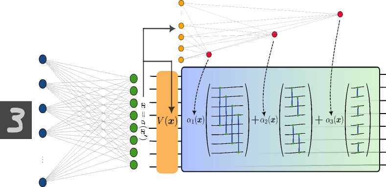
i

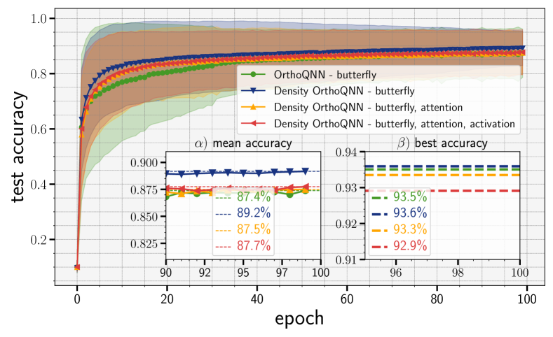
ii

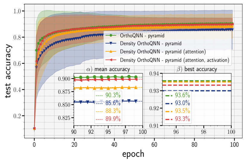
iii

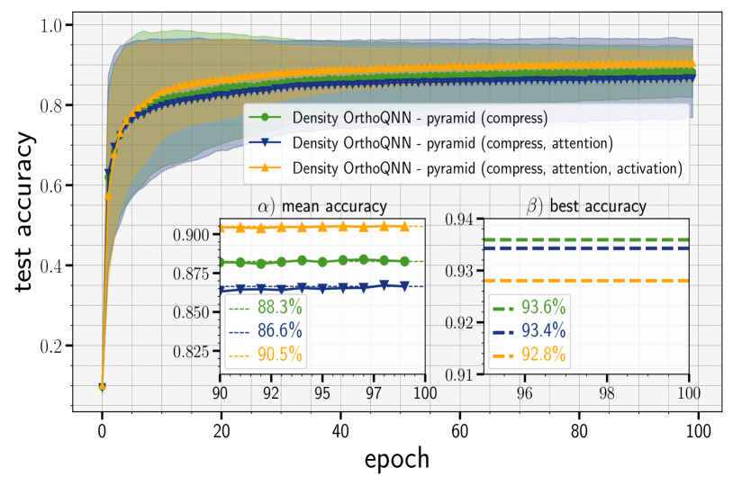
iv

Figure 7: Density QNN with data dependent sub-unitary weighting parameters.
i) "Attention"-like mechanism to learn distribution of sub-unitaries in a data dependent manner, for the decomposed butterfly OrthoQNN. A simple linear layer takes as input $\boldsymbol{x}:=\sigma(\boldsymbol{x}^{\prime})$, and outputs $\boldsymbol{\alpha}(\boldsymbol{x})=\{\boldsymbol{\alpha}_{k}(\boldsymbol{x})\}$, again with $\sum_{k}\boldsymbol{\alpha}_{k}(\boldsymbol{x})=1\leavevmode\nobreak\ \forall\boldsymbol{x}$. We omit the final (classical) post-processing layer. We test this for the ii) butterfly decomposition, iii) pyramid decomposition (compressed) and iv) pyramid decomposition. Again, we perform hyperparameter optimisation over $32$ trails. We notice, for those models which are very ‘shallow’, or have few parameters - namely the butterfly and the compressed pyramid extraction, data dependence in the trainable distribution does not seem to help performance. However, if we have a larger number of parameters as in the even-odd extraction of the pyramid circuit (see Fig. 6i in the main text), ‘attention’ (data-dependent learnable weighted distribution) does appear to help the model learn, achieving both a higher absolute test accuracy over all hyperparameters, and a better average accuracy, with a smaller standard deviation.

The attention mechanism is, at its core, a method to focus on specific parts of the input data that are most relevant to the task at hand. In the case of sequence to sequence models [50] this is parameterised as a weighted average of relationships between input and output sequences, by learning correlations between them. Each element in the output sequence learns to “attend" to the part(s) of the input sequence which most impacts it. In a simple case, a distribution over possible relationships is created, which the most likely correlations having the highest weighting.

Here, we can view the DenQNN as an attention mechanism in the following form. The distribution of sub-unitaries, $\alpha_{j}$, act as a weighting over sub-unitaries. If the method of parameterising the distribution is efficient and (efficiently) trainable, the model will select the sub-unitary which is most effective at extracting information from the data.

For example, in quantum data applications, one could imagine classifying directly states corresponding to fixed $k$-body Hamiltonians, as in the quantum phase recognition problem [46]. A sequence of sub-unitaries could be defined with specific entangling characteristics: $U_{1}$ contains only $1$-body terms (single qubit rotations), $U_{2}$ contains $2$-body terms (two qubit gates), $U_{3}$ contains $3$-body terms and so on. We create a DenQNN with probabilities $\{\alpha_{1},\alpha_{2},\alpha_{3},\dots\}$. It is clear that if the state to be classified is a product state, then the model is sufficient to learn the weighting $\alpha_{1}=1,\alpha_{j}=0\leavevmode\nobreak\ \forall j\neq 1$, which conversely will not be sufficient for more strongly entangled inputs.

In reality, what we aim to do is inject a data dependence into the trainable distribution of sub-unitaries, $\boldsymbol{\alpha}\rightarrow\boldsymbol{\alpha}(\boldsymbol{x})$. Any true analogue to any particular classical attention procedure is superficial. This is because, classically, a given attention mechanism will be a problem dependent operation. Though, this is even true between two types of purely classical attention mechanisms - the only commonality between attention used in language processing [51] versus those used in certain time series applications (e.g. [52]) is the use of a softmax function to create a distribution over possibilities, which we similarly do here.

4.3.3   Logarithmic butterfly decomposition

Now, we move to the butterfly decomposition for a density QNN, and test the effectiveness of the attention mechanism for this model, along with the even-odd decomposition from Section 4.3.1.

It is clear that from the butterfly Fig. 2c) on $8$ qubits, we can decompose into $\log_{2}(8)=3$ sub-unitaries. We show this in Fig. 7i. For a general butterfly layer on $n$ qubits, we can construct a density model with $\log_{2}(n)$ sub-unitaries. This gives a gradient scaling advantage from $\mathcal{O}(n\log(n))$ (butterfly OrthoQNN) to $\mathcal{O}(\log(n))$(density butterfly extraction) for the same reason as the even-odd extraction.

For the attention weighting, $\{\alpha_{1}(\boldsymbol{x}),\alpha_{2}(\boldsymbol{x}),\alpha_{3}(\boldsymbol{x})\}$ we use a simple linear layer to map from the output of the feature extractor, $\sigma(\boldsymbol{x}^{\prime})$ to the distribution $\boldsymbol{\alpha}(\boldsymbol{x})$ via a softmax (denoted “attention” in Fig. 7) along with a version including a non-linear activation (denoted “attention, activation”) before the softmax. We again test using MNIST data for the butterfly (Fig. 7ii), odd-even (Fig. 7iii) and compressed odd-even (Fig. 7iv) respectively, again plotting the accuracy averaged over hyperparameter runs (insets $\alpha$) and best accuracy (insets $\beta$) over all hyperparameters.

“attention”

$$\implies\alpha_{k}(\boldsymbol{x})=\texttt{softmax}_{k}(\texttt{Linear}(\sigma(\boldsymbol{x}^{\prime})),$$

“attention, activation”

$$\implies\alpha_{k}(\boldsymbol{x})=\texttt{softmax}_{k}(\mathsf{GELU}(\texttt{Linear}(\sigma(\boldsymbol{x}^{\prime})))$$

We make some observations for these results. First, in some cases, the vanilla density model can outperform it’s pure version, e.g. comparing best accuracy achieved by the DenQNN-butterfly versus the OrthoQNN-butterfly in Fig. 7ii$\beta)$. Second, for models with larger parameter counts per sub-unitary, e.g. the uncompressed even-odd decomposition, the data-dependent attention does appear to help (with/without activation) - and can boost performance to the level of the original model. Third, an explicit activation function does not have a conclusive impact in performance - it can make the model perform better on average over hyperparameter optimisation as in Figs. 7iii$\alpha)$, 7iv$\alpha)$, but ultimately the best accuracies are found either by the original model or the density model without activation ($\beta)$). The final observation is that making $\boldsymbol{\alpha}(\boldsymbol{x})$ data dependent, and predictable by a neural network, reduces the variance of the training over hyperparameter runs, which can be observed in all scenarios. This is perhaps not surprising as the classical model is able to act as a more effective teacher for the student (density) model.

4.3.4   Linear round-robin decomposition

To make the model even more expressive past the butterfly extraction, we can decompose into a so-called round-robin decomposition [17] which brings the number of quantum trainable parameters in line with that of a full orthogonal transformation (as in the pyramid decomposition), see Fig. 8ii. Specifically, to construct this decomposition using RBS gates, we iterate over distances, $k\in\{1,\dots,\frac{n}{2}\}$, and choose all pairs of qubits for each $k$. The round-robin decomposition reflects an all-to-all graph connectivity since the (weighted) sum of all these unitaries can establish a connection from any qubit $i$ to any other $j,\forall i,j\in[1,n]$. As a result, the density round-robin consists of $n-1$ commuting generator circuits, each containing $\frac{n}{2}$ parameters, giving $\frac{n(n-1)}{2}$ parameters overall, matching the number in a pyramid circuit. Of course, this reflects only in a mapping from the input encoded vectors, $\boldsymbol{x}$, to the output vectors, $\boldsymbol{y}$, not a mapping between any input state $\ket{\psi}$ and any other $\ket{\phi}$. We compare the density round-robin model to the pyramid ortholinear layer in 8ii. We remove the linear layers before and after both quantum models to test directly the expressive power of each. After optimising over the hyperparameters described in App. F.1, the best performing density QNN model with a round-robin decomposition outperforms the pyramid orthogonal quantum neural network, by a substantial margin of $\sim 4\%$, and also converges in significantly fewer epochs. We use the full MNIST dataset with $60,000$ train and $10,000$ test images and downscale each image to $16$ qubits using principal component analysis.

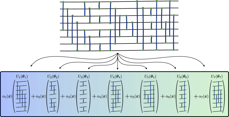
i

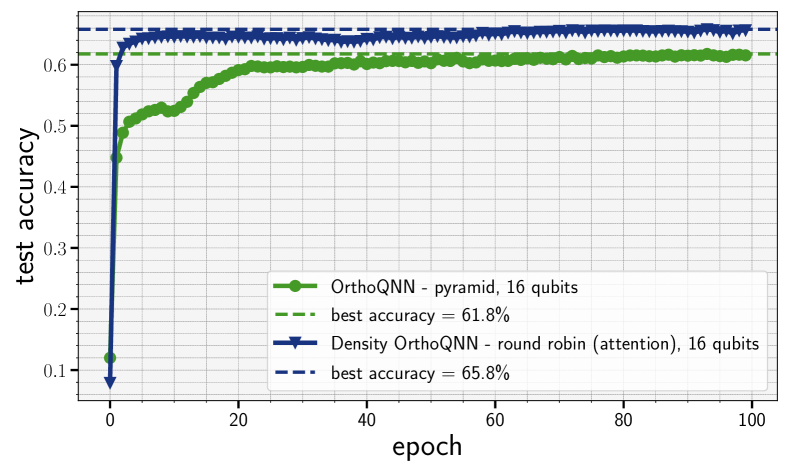
ii

Figure 8: Round-robin OrthoQNN and decomposition into a round-robin density QNN.
8i) An example of the ‘round-robin’ decomposition of an orthogonal quantum neural network with $n=8$ qubits, requiring $7$ ($=n-1$) sub-unitaries to form the density version (bottom) using RBS gates. The round-robin decomposition requires $n(n-1)/2$ parameters and creates an effective all-to-all connectivity relating input vectors $\boldsymbol{x}$ to output vectors $\boldsymbol{y}$. A corresponding single-unitary round-robin OrthoQNN can be created by applying $U_{1},\dots U_{7}$ sequentially on the input state (top). 8ii) Comparison on MNIST of the round-robin density QNN to a pyramid decomposition 2a). Here we do not use pre- and post– processing linear layers, but simply input raw data into both models and take the outputs directly as the classification vector. We downsize the MNIST images to $16$ dimensional vectors to unary-amplitude-encode into $16$ qubits. Again, for the Density QNN, we train data dependent ‘attention’ coefficients, $\{\alpha_{k}(\boldsymbol{x})\}_{k=1}^{15}$, for the $15$ round robin unitaries. Plots show the best result for both models over $16$ independent hyperparameter runs.

5   Discussion

The search for quantum machine learning models which are efficiently trainable, especially on quantum hardware, is key to the success of the field. Expressivity, non-vanishing gradients and inductive biases are important aspects of quantum models which have been relatively well studied in the literature, however, gradient scaling has received comparatively less attention. In this work, we proposed density quantum neural networks - a particular generalisation of the commonly used ‘pure’ parameterised quantum circuit learning models. We showed that the gradients of this model depend on the complexity of the gradient evaluation of the model’s component sub-unitaries. Choosing these sub-unitaries to be commuting-block circuits leads to a constant number of gradient circuits required but the overall density model is potentially more expressive. On the other hand, inspired by an interpretable and well defined model such as the orthogonal quantum neural network, we can define a density counterpart which in some cases can outperform the original, with a significant (theoretical) reduction in overall training time. In this latter case, we demonstrated numerically that this scaling advantage does not lead to a substantial drop in model quality. There are a number of avenues which could be explored in future work. The primary two are: the study of the expressivity of the density QNN model when different families of sub-unitaries are used, and searching for other sub-unitary families which are trainable efficiently. If such examples are found, they can immediately be uplifted to the density model as a consequence of the results in this paper (as in the hardware efficient QNN example). A third interesting direction is the efficient classical simulability of the density quantum neural networks in specific cases.

Appendix A Training orthogonal quantum neural networks

As mentioned in the main text, orthogonality of weight matrices is a desirable feature in classical machine learning, but is difficult to maintain while training via gradient descent. To combat this, orthogonality preserving methods include: 1) projecting to the Stiefel manifold (the manifold of orthogonal matrices) via, e.g. singular value decompositions (SVDs), 2) performing gradient descent directly in the space of orthogonal matrices, 3) exponentiation and optimisation of an anti-symmetric generator matrix or 4) adding orthogonality regularisation terms to the loss function to be optimised. The first three techniques are theoretically expensive, typically using $\mathcal{O}(n^{3})$ complexity to orthogonalise an $n\times n$ weight matrix, while the latter regularisation technique will only enforce approximate orthogonality.

Orthogonal quantum neural networks (OrthoQNNs) were proposed by Ref. [12] as an alleviation to this, and have two possible ‘modes’ of operation for machine learning purposes. The first mode is in a quantum-inspired (classical) mode where they can be used as completely classical models for orthogonal neural networks. This is due to the special nature of the gates used within the circuits - specifically all operations within an OrthoQNN are Hamming weight (HW) preserving, inheriting the property from the underlying RBS or FBS gates. Applied on a unary data encoding, $\ket{\psi}_{\mathsf{unary}}=\sum_{i=1}^{n}x_{i}\ket{e_{i}},e_{j}:=00\cdots 1_{j}\cdots 00$), an OrthoQNN, $\ket{\phi}_{\mathsf{unary}}=U_{\mathsf{pyr}}(\boldsymbol{\theta})\ket{\psi}_{\mathsf{unary}}$, will preserve the unary nature of the input so $\ket{\phi}_{\mathsf{unary}}$ will also be exclusively supported on the $n$ unary basis elements. This restriction to an $n$ dimensional subspace enables efficient classically simulability, depending on the input state. Therefore, they can also be trained in a purely classical mode without an exponential overhead. A method for performing layerwise (on those subsets of gates which can be applied in a single timestep, or moment, in parallel - see 6ia) for an example of such a decomposition) training classically was proposed also in [12] which enables the incorporation of such layers in backpropagation pipelines, with an overhead scaling with the number of layers ($\mathcal{O}(n)$ for the pyramid/round-robin circuits or $\mathcal{O}(\log(n))$ for the butterfly circuit).

The second mode is the fully ‘quantum’ mode - where the orthogonal layers are evaluated and trained on quantum hardware. Here, automatic differentiation through layers is not possible as in the classical scenario, and one must resort to the $\mathcal{O}(n^{2})$ parameter-shift rule. Is it possible to have a method scaling as the classical $\mathcal{O}(n)$ layerwise training? If we could apply the commuting-block argument of Ref. [15], this would be achievable.

However, this is not straightforward - the gates within a layer obviously commute (since they act on different qubits), but RBS gates between layers do not obey the required fixed commutation relation. This is because the generators of two RBS which share a single qubit neither completely commute nor anticommute, which can be seen as follows with two RBS gates, acting on qubits $0,1$ ($G_{a}$) and $1,2$ ($G_{b}$):

$$G_{a} :=\textsf{Y}_{0}\otimes\textsf{X}_{1}\otimes\mathds{1}_{2}-\textsf{X}_{0}\otimes\textsf{Y}_{1}\otimes\mathds{1}_{2},\qquad G_{b}:=\mathds{1}_{0}\otimes\textsf{Y}_{1}\otimes\textsf{X}_{2}-\mathds{1}_{0}\otimes\textsf{X}_{1}\otimes\textsf{Y}_{2}$$

$$G_{a}\times G_{b} =\textsf{Y}_{0}\otimes\textsf{X}_{1}\textsf{Y}_{1}\otimes\textsf{X}_{2}-\textsf{X}_{0}\otimes\textsf{Y}_{1}\textsf{Y}_{1}\otimes\textsf{X}_{2}-\textsf{Y}_{0}\otimes\textsf{X}_{1}\textsf{X}_{1}\otimes\textsf{Y}_{2}+\textsf{X}_{0}\otimes\textsf{Y}_{1}\textsf{X}_{1}\otimes\textsf{Y}_{2}$$

$$=G_{\text{comm}}+G_{\text{anti-comm}}$$

So we have a commuting part ($\textsf{X}_{1}\textsf{X}_{1}$ or $\textsf{Y}_{1}\textsf{Y}_{1}$) and an anti-commuting part ($\textsf{X}_{1}\textsf{Y}_{1}$ or $\textsf{Y}_{1}\textsf{X}_{1}$) on the shared qubit. As a result, $[G_{a},G_{b}]=2G_{\text{anti-comm}}\neq 0$ and similarly $\{G_{a},G_{b}\}$ does not vanish. We leave a search for an efficient OrthoQNN specific training protocol to future research, and in the next sections focus on the parameter-shift rule.

A.1   Parameter-shift rule for OrthoQNNs

Here, we show the circuits required for computing gradients of the OrthoQNN ansätze in Fig. 2 in the main text. Since all gates in these circuits are simply RBS gates, we need only to compute the parameter-shift for the RBS gate.

This result has been derived before [55] in the context of fermionic quantum simulation, but we include it here for completeness, and to explicitly keep track of constant factors due to our slightly different parameterisation of the RBS gate. Specifically the general gate in Ref. [55] is defined as $\exp\left(-i\theta/2Q\right)$ whereas we define the RBS gate in the form $\exp\left(-i\theta Q\right)$. This factor does not matter in practice for training such models, as the optimiser can adapt the parameters accordingly, but it is important for debugging purposes to generate the correct formulae for the appropriate gates. We also assume the output of the model is the expectation values of Hermitian observables, $\mathcal{B}_{0}$ relative to a single pure state created by a sequence of unitaries, We can also assume a data encoding with unitary $V(\boldsymbol{x}),\ket{\boldsymbol{x}}:=V(\boldsymbol{x})\ket{0}^{\otimes n}$:

$$f(\boldsymbol{\theta}) =\bra{\psi(\theta,\boldsymbol{x})}\mathcal{B}_{0}\ket{\psi(\theta,\boldsymbol{x})}=\bra{\boldsymbol{x}}U^{\theta_{1}\dagger}\cdots U^{\theta_{j}\dagger}\cdots U^{\theta_{J-1}\dagger}U^{\theta_{J}\dagger}\mathcal{B}_{0}U^{\theta_{J}}U^{\theta_{J-1}}\cdots U^{\theta_{i}}\cdots U^{\theta_{1}}\ket{\boldsymbol{x}}$$ (18)

$$=\bra{\boldsymbol{x}}\mathcal{U}^{\dagger}_{[1:j]}(\theta)\mathcal{B}_{[j+1:J]}\mathcal{U}_{[1:j]}(\theta)\ket{\boldsymbol{x}}$$

$$\mathcal{B}_{[j+1:J]} :=U^{\theta_{j+1}\dagger}\cdots U^{\theta_{J-1}\dagger}U^{\theta_{J}\dagger}\mathcal{B}_{0}U^{\theta_{J}}U^{\theta_{J-1}}\cdots U^{\theta_{j+1}}$$

Each RBS gate is of the form $\textsf{RBS}(\theta)=U(\theta)=\exp\left(-i\theta Q\right)$ with $Q:=1/2\left(\textsf{Y}\otimes\textsf{X}-\textsf{X}\otimes\textsf{Y}\right)$. This generator has the property that $Q^{3}=Q$ and has eigenvalues $\{0,\pm 1\}$. Therefore, according to [9, 55] we can write $U(\theta)$ as:

$$U(\theta)=\mathds{1}+\left(\cos(\theta)-1\right)Q^{2}-i\sin\left(\theta\right)Q$$

Following the logic of Ref. [55], the expression for the gradient with respect to $\theta$ will involve the commutator, $[\mathcal{B},Q]$ (suppressing the indices on $\mathcal{B})$:

$$\frac{\partial f(\boldsymbol{\theta})}{\partial\theta}=\bra{\boldsymbol{x}}\mathcal{U}^{\dagger}_{[1:j]}(\theta)\left(-i[\mathcal{B}_{[j+1:J]},Q]\right)\mathcal{U}_{[1:j]}(\theta)\ket{\boldsymbol{x}}$$ (19)

Defining, $U(\theta)(\mathcal{B}):=U^{\dagger}(\theta)\mathcal{B}U(\theta)$ so:

$$U(\pm\theta)(\mathcal{B}) =\left[\mathcal{B}+\left(\cos(\theta)-1\right)Q^{2}\mathcal{B}\pm i\sin\left(\theta\right)Q\mathcal{B}\right]\left[\mathds{1}+\left(\cos(\theta)-1\right)Q^{2}\mp i\sin\left(\theta\right)Q\right]$$

$$:=\left[\mathcal{B}+\delta Q^{2}\mathcal{B}\pm\gamma QB\right]\left[\mathds{1}+\delta Q^{2}\mp\gamma Q\right]$$

$$=\mathcal{B}+\delta\mathcal{B}Q^{2}\mp\gamma\mathcal{B}Q+\left[\delta Q^{2}\mathcal{B}+\delta^{2}Q^{2}\mathcal{B}Q^{2}\mp\gamma\delta Q^{2}\mathcal{B}Q\right]+\left[\pm\gamma Q\mathcal{B}\pm\delta\gamma Q\mathcal{B}Q^{2}-\gamma^{2}Q\mathcal{B}Q\right]$$

It turns out that we can extract the commutator above by taking linear combinations of the following $U(\theta)(\mathcal{B})-U(-\theta)(\mathcal{B})$ for different values of the angles. Computing this term gives:

$$U(\theta)(\mathcal{B})-U(-\theta)(\mathcal{B}) =-2\gamma\mathcal{B}Q-2\gamma\delta Q^{2}BQ+2\gamma QB+2\delta\gamma QBQ^{2}$$

$$=-2\gamma[\mathcal{B},Q]-2\delta\gamma[Q,Q\mathcal{B}Q]$$

$$=-2i\sin\left(\theta\right)[\mathcal{B},Q]-2i\sin\left(\theta\right)\left(\cos\left(\theta\right)-1\right)[Q,Q\mathcal{B}Q]$$

Evaluating the commutator by taking a linear combination of the above expression with two different angles, $\pm\alpha,\pm\beta$ gives:

$$-i[\mathcal{B},Q]= d_{1}\left[U(\alpha)(\mathcal{B})-U(-\alpha)(\mathcal{B})\right]-d_{2}\left[U(\beta)(\mathcal{B})-U(-\beta)(\mathcal{B})\right]$$

$$= d_{1}(-2i\sin\left(\alpha\right)[\mathcal{B},Q]-2i\sin\left(\alpha\right)\left(\cos\left(\alpha\right)-1\right)[Q,Q\mathcal{B}Q])$$

$$+d_{2}(2i\sin\left(\beta\right)[\mathcal{B},Q]+2i\sin\left(\beta\right)\left(\cos\left(\beta\right)-1\right)[Q,Q\mathcal{B}Q])$$

$$= -i[\mathcal{B},Q]\left(2d_{1}\sin\left(\alpha\right)-2d_{2}\sin\left(\beta\right)\right)-2i[Q,Q\mathcal{B}Q]\left[d_{1}\sin\left(\alpha\right)\left(\cos\left(\alpha\right)-1\right)-d_{2}\sin\left(\beta\right)\left(\cos\left(\beta\right)-1\right)\right]$$

The coefficient of $[\mathcal{B},Q]$ should $=1$, while the coeffecient of $[Q,Q\mathcal{B}Q]$ should $=0$. Therefore, we get the conditions:

$$2d_{1}\sin\left(\alpha\right)-2d_{2}\sin\left(\beta\right)=1 \implies d_{1}\sin\left(\alpha\right)-d_{2}\sin\left(\beta\right)=\frac{1}{2}$$

$$d_{1}\sin\left(\alpha\right)\left(\cos\left(\alpha\right)-1\right)-d_{2}\sin\left(\beta\right)\left(\cos\left(\beta\right)-1\right)=0 \implies d_{1}\sin\left(2\alpha\right)-d_{2}\sin\left(2\beta\right)=1$$

To solve these, we can take $d_{1}=1,d_{2}=\frac{(\sqrt{2}-1)}{2},\alpha=\frac{\pi}{4}$ and $\beta=\frac{\pi}{2}$ Then we arrive at a four term gradient rule for RBS gates:

$$\frac{\partial f(\boldsymbol{\theta})}{\partial\theta_{i}}=\left[f\left(\theta_{i}+\frac{\pi}{4}\right)-f\left(\theta_{i}-\frac{\pi}{4}\right)\right]-\frac{\sqrt{2}-1}{2}\left[f\left(\theta_{i}+\frac{\pi}{2}\right)-f\left(\theta_{i}-\frac{\pi}{2}\right)\right]$$ (20)

A.2   Parameter-shift rule for FBS gates

A useful generalisation of the RBS gates defined in the main text is to so-called Fermionic beam splitter [37] (FBS) gates, which are defined as follows:

$$\textsf{FBS}(\theta)_{ij}\ket{\boldsymbol{s}}=\\ \left(\begin{array}[]{cccc}1&0&0&0\\ 0&\cos(\theta)&(-1)^{f_{i,j,\boldsymbol{s}}}\sin(\theta)&0\\ 0&(-1)^{f_{i,j,\boldsymbol{s}}+1}\sin(\theta)&\cos(\theta)&0\\ 0&0&0&1\end{array}\right)$$ (21)

The FBS gate acts on two qubits, $i,j$, and is defined along with the overall $n$ computational basis state $\boldsymbol{s}\in\{0,1\}^{n}$ it acts on. Here, $f_{i,j,\boldsymbol{s}}:=f(i,j,\boldsymbol{s}):=\sum_{i<k<j}s_{k}$. If the parity, $\bigoplus_{i<k<j}s_{k}$ between qubits $i,j$ is odd, we have $\textsf{FBS}(\theta)=\textsf{RBS}(\theta)$ gate, and equal to $\textsf{RBS}(-\theta)$ otherwise. FBS gates, in contrast to the strictly two-local RBS gates may generally be maximally non-local acting on all qubits at once, due to need to compute the parity term $f_{i,j,\boldsymbol{s}}$ quantumly. The FBS gates in particular are useful in creating subspace states [37], a useful primitive that can, for example, accelerate determinant sampling machine learning methods [56, 57]. Finally, as mentioned in the main text, applying such FBS gates on higher order Hamming-weight initial states, or superpositions of different Hamming-weight states results in compound matrices of order $k$ acting on the $\binom{n}{k}$ dimensional Hamming-weight $k$ subspace.

How does one then train these FBS gates with a version of the parameter shift rule? This is perhaps not obvious at a first glance as from eq. (21) as it is not trivial to write as a single operation of the form $e^{i\theta G}$ for some Hermitian generator $G$, and if we did so, $G$ would be a multi-qubit operation.

However, using the correspondence between the FBS and the RBS gate from Ref. [37], it becomes clear that one can simply derive the parameter-shift rule for an FBS gate from that of an RBS gate, and it turns out to have the same functional form as eq. (20). This fact means that if, on quantum hardware, one has a native way to implement FBS gates (which are generally non-local), evaluating the gradients of these gates does not require any extra circuit resources over simply evaluating the function itself. One may simply compute gradients using the same FBS gates but with shifted parameters, even though the FBS gate itself is not in an obvious form for the parameter-shift requirements. If the FBS gate instead decomposed into a primitive with perhaps multiple RBS gates (but each with some fraction of the total angle), this fact may not materialise.

The correspondence is the following (Proposition 2.6 in Ref. [37]):

$$\textsf{FBS}(\theta)_{ij}=\mathcal{P}(i+1,j)\textsf{CZ}_{i+1,j}\textsf{RBS}(\theta)_{ij}\textsf{CZ}_{i+1,j}\mathcal{P}^{\dagger}(i+1,j)$$ (22)

where $\mathcal{P}(i+1,j)$ is a circuit which computes the parity of the qubits $k$ qubits between $i$ and $j$ into qubit $i+1$, such that $|i-j|=k+1$.

Then let $f_{\textsf{FBS}}(\boldsymbol{\theta})$ be the function implemented by a quantum circuit with trainable parameters in FBS gates. We have

$$\frac{\partial f_{\textsf{FBS}}(\boldsymbol{\theta})}{\partial\theta_{i}} =\left[f^{\prime}_{\textsf{RBS}}\left(\theta_{i}+\frac{\pi}{4}\right)-f^{\prime}_{\textsf{RBS}}\left(\theta_{i}-\frac{\pi}{4}\right)\right]-\frac{\sqrt{2}-1}{2}\left[f^{\prime}_{\textsf{RBS}}\left(\theta_{i}+\frac{\pi}{2}\right)-f^{\prime}_{\textsf{RBS}}\left(\theta_{i}-\frac{\pi}{2}\right)\right]$$

$$=\left[f_{\textsf{FBS}}\left(\theta_{i}+\frac{\pi}{4}\right)-f_{\textsf{FBS}}\left(\theta_{i}-\frac{\pi}{4}\right)\right]-\frac{\sqrt{2}-1}{2}\left[f_{\textsf{FBS}}\left(\theta_{i}+\frac{\pi}{2}\right)-f_{\textsf{FBS}}\left(\theta_{i}-\frac{\pi}{2}\right)\right]$$

where $f^{\prime}_{\textsf{RBS}}$ is the formally-equivalent circuit to $f_{\textsf{FBS}}(\boldsymbol{\theta}$, but replacing all $\textsf{FBS}(\theta)_{ij}$ with the expressions using RBS gates eq. (22). In other words, we take the FBS circuit, write all FBS in terms of corresponding RBS gates and gates with no parameters, evaluate the gradients with respect to the RBS parameters - which end up as circuits with identical form, but with simply shifted parameters - then rewrite the RBS circuits back in the form of FBS gates (shifted by the same amount), again using the relation above.

Appendix B Proofs

B.1   Proof of Proposition 1

Proposition (Gradient scaling for density quantum neural networks (Proposition 1 repeated) ).

Given a density QNN as in eq. (10) composed of $K$ sub-unitaries, $\mathcal{U}=\{U_{k}(\boldsymbol{\theta}_{k})\}$, implemented with distribution, $\boldsymbol{\alpha}=\{\alpha_{k}\}$, an unbiased estimator of the gradients of a loss function, $\mathcal{L}$, defined by a Hermitian observable, $\mathcal{H}$:

$$\mathcal{L}(\boldsymbol{\theta},\boldsymbol{\alpha},\boldsymbol{x})=\Tr\Big(\mathcal{H}\rho(\boldsymbol{\theta},\boldsymbol{\alpha},\boldsymbol{x})\Big{missing})$$ (23)

can be computed by classically post-processing $\sum_{l=1}^{K}\sum_{k=1}^{K}T_{\ell k}$ circuits, where $T_{\ell k}$ is the number of circuits required to compute the gradient of sub-unitary $k$, $U(\boldsymbol{\theta}_{k})$ with respect to the parameters in sub-unitary $\ell$, $\boldsymbol{\theta}_{\ell}$. Furthermore, these parameters can also be shared across the unitaries, $\boldsymbol{\theta}_{k}=\boldsymbol{\theta}_{k^{\prime}}$ for some $k,k^{\prime}$.

Proof.

Assume for simplicity that the number of parameters in each sub-unitary is the same, $B_{k}=B\leavevmode\nobreak\ \forall k$ and $N_{B_{k}}=N_{B}=N$. Furthermore assume the number of blocks is $B=1$. Then for notational purposes we can write the following $K\times K\times N$ tensor, with the $j^{th}$ ‘slice’ across the last dimension being:

$$[\Delta\mathcal{L}(\boldsymbol{\theta},\boldsymbol{\alpha},\boldsymbol{x})]_{j}:=\left(\begin{array}[]{ccc}\partial_{j1}\mathcal{L}^{\prime}(\boldsymbol{\theta}_{1},\boldsymbol{x})&\cdots&\partial_{jK}\mathcal{L}^{\prime}(\boldsymbol{\theta}_{1},\boldsymbol{x})\\ \vdots&\ddots&\vdots\\ \partial_{j1}\mathcal{L}^{\prime}(\boldsymbol{\theta}_{K},\boldsymbol{x})&\cdots&\partial_{jK}\mathcal{L}^{\prime}(\boldsymbol{\theta}_{K},\boldsymbol{x})\end{array}\right)$$ (24)

where $\mathcal{L}^{\prime}$ is the loss function evaluated using only a single term of the density sum:

$$\mathcal{L}^{\prime}(\boldsymbol{\theta}_{k},\boldsymbol{x}) :=\Tr\Big(\mathcal{H}U_{k}(\boldsymbol{\theta}_{k})\outerproduct{\boldsymbol{x}}{\boldsymbol{x}}U^{\dagger}_{k}(\boldsymbol{\theta}_{k})\Big{missing})$$

$$\implies\partial_{\ell}\mathcal{L}^{\prime}(\boldsymbol{\theta}_{k},\boldsymbol{x}) :=\frac{\partial\mathcal{L}^{\prime}(\boldsymbol{\theta}_{k},\boldsymbol{x})}{\partial\boldsymbol{\theta}_{\ell}},\partial_{j\ell}\mathcal{L}^{\prime}(\boldsymbol{\theta}_{k},\boldsymbol{x}):=\frac{\partial\mathcal{L}^{\prime}(\boldsymbol{\theta}_{k},\boldsymbol{x})}{\partial\theta^{j}_{\ell}}$$

In other words, the $j^{th}$ slice of $\Delta\mathcal{L}(\boldsymbol{\theta},\boldsymbol{\alpha},\boldsymbol{x})$ is a matrix, where the rows and columns are indexed by the terms in the model eq. (10) - the diagonal terms are the gradients of the $k^{th}$ sub-unitary with respect to the $k^{th}$ set of parameters, while the off-diagonal terms are the gradients of the $k^{th}$ term with respect to the $\ell^{th}$ ($\ell\neq k$) set of parameters.

Now, we can plug in the definition of the model (eq. (10)), taking the gradient w.r.t the $k^{th}$ sub-unitaries parameters (a vector of size $N$):

$$\left[\frac{\partial\mathcal{L}(\boldsymbol{\theta},\boldsymbol{\alpha},\boldsymbol{x})}{\partial\boldsymbol{\theta}_{\ell}}\right]_{j}=\frac{\partial\Tr\Big(\mathcal{H}\rho(\boldsymbol{\theta},\boldsymbol{\alpha},\boldsymbol{x})\Big{missing})}{\partial\theta^{j}_{\ell}}=\sum_{k=1}^{K}\alpha_{k}\frac{\partial\Tr\Big(\mathcal{H}U_{k}(\boldsymbol{\theta}_{k})\outerproduct{\boldsymbol{x}}{\boldsymbol{x}}U^{\dagger}_{k}(\boldsymbol{\theta}_{k})\Big{missing})}{\partial\theta^{j}_{\ell}}\\ =\sum_{k=1}^{K}\alpha_{k}\partial_{j\ell}\mathcal{L}^{\prime}(\boldsymbol{\theta}_{k},\boldsymbol{x})=\sum_{k=1}^{K}\alpha_{k}[[\Delta\mathcal{L}(\boldsymbol{\theta},\boldsymbol{\alpha},\boldsymbol{x})]_{j}]_{\ell,k}$$ (25)

where $[[\Delta\mathcal{L}(\boldsymbol{\theta},\boldsymbol{\alpha},\boldsymbol{x})]_{j}]_{\ell,k}$ is the $\ell,k$ element of eq. (24). Hence, assuming we can compute the $k^{th}$ column of $\Delta\mathcal{L}(\boldsymbol{\theta},\boldsymbol{\alpha},\boldsymbol{x})$ with $T_{k}$ circuits, we can estimate eq. (25) by computing the gradient with respect to each sub-unitary $U_{k}$ and summing the resulting (weighted by $\alpha_{k}$) vectors. ∎

As discussed in the main text, there are two sub-cases one can consider. First, if all parameters between sub-unitaries are independent, $\boldsymbol{\theta}_{k}\neq\boldsymbol{\theta}_{\ell},\leavevmode\nobreak\ \forall k,\ell$. Here, the computation is simpler as taking a gradient with respect to the parameters of sub-unitary, $U_{k}$, results in all other columns of eq. (24) vanishing, i.e. $[[\Delta\mathcal{L}(\boldsymbol{\theta},\boldsymbol{\alpha},\boldsymbol{x})]_{j}]_{\ell,k}=0,\leavevmode\nobreak\ \forall\ell\neq k$. Hence, we only need to extract the diagonal terms from eq. (24), $\partial_{jk}\mathcal{L}^{\prime}(\boldsymbol{\theta}_{k},\boldsymbol{x})$ for each $j$. This observation then gives 1 in the main text.

Appendix C Measurement protocol & gradients for orthogonal QNNs

In the main text, it was stated that the gradients of all orthogonal-inspired density QNNs could be evaluated more quickly than their OrthoQNN counterparts. However, to adapt Theorem 1 of Ref. [15] fully, we require the generators commute and the measurement operator obeys the commutation relation specified therein. We will see how this raises a subtlety not addressed in previous works.

Since $\boldsymbol{y}$ is also a unary encoding, to fully extract the state we only need $n$ amplitudes - those corresponding to the unary bitstrings, $\boldsymbol{e}_{j}:=0\cdots 1_{j}\cdots 0$. This can be done using an $\ell_{\infty}$-norm tomography procedure [58, 12] as follows. Firstly, the probabilities of the unary states are extracted, $p(\boldsymbol{e}_{j}):=y_{j}^{2}$ via direct measurement of the circuit. Then two auxiliary circuits are evaluated to extract the signs of the amplitudes. These first/second appends a layer of $\textsf{RBS}(\frac{\pi}{4})$ gates onto the odd/even-controlled qubits after the OrthoQNN, (see Figure 18 in [12] for details). The three circuits are measured in the Pauli Z basis to extract the final amplitudes $y_{j}$. While stated in previous works that it is sufficient to measure all simultaneously in the Z basis to extract the unary amplitudes, we show in the following section this is not true if one is also interested in hardware trainability. We must be more careful in the measurement protocol.

Focusing on probability extraction, $p(\boldsymbol{e}_{j}):=y_{j}^{2}$ (the sign evaluation follows similar logic) we have three choices, which impact practicality and trainability. We can $1)$ measure $\mathds{1}^{\otimes(j-1)}\otimes\textsf{Z}_{j}\otimes\mathds{1}^{\otimes(n-j)}$ on each qubit individually, $2)$ perform a global measurement, $\textsf{Z}^{\otimes(j-1)}\otimes\textsf{Z}_{j}\otimes\textsf{Z}^{\otimes(n-j)}$ over all qubits at once or $3)$ measure non-overlapping qubit pairs $\mathds{1}_{1}\otimes\textsf{Z}_{2}\otimes\mathds{1}_{3}\otimes\textsf{Z}_{4}\dots\mathds{1}_{n-1}\otimes\textsf{Z}_{n}$ (or equivalently swapping $\mathds{1}\leftrightarrow\textsf{Z}$ for each pair). In terms of forward passes, option $(1)$ adds an $\mathcal{O}(n)$ complexity, while options $2/3)$ add an $\mathcal{O}(1)$ complexity (option $(2)$ requires only a single circuit to run, while option $(3)$ requires $2$ circuits, one to characterise $\mathds{1}_{j}\otimes\textsf{Z}_{j+1}$ and the other for $\textsf{Z}_{j}\otimes\mathds{1}_{j+1}$ for each pair, $\{j,j+1\}$. In all cases, the probabilities are estimated by counting the number of ‘$1$’s on each qubit, $j$. However, while each technically resolves the same information (the probabilities of the unary states), there is a fundamental difference with respect to trainability.

The commuting nature of the generators, $G_{j}\propto\textsf{Y}_{j_{1}}\otimes\textsf{X}_{j_{2}}-\textsf{X}_{j_{1}}\otimes\textsf{Y}_{j_{2}}$ enables us to apply the results of Ref. [15] if the measurement Hamiltonian, $\mathcal{H}$ either commutes or anticommutes with $G_{j}$. If $\mathcal{H}$ commutes, $[\mathcal{H},G_{j}]=0$ and therefore the gradient expression in eq. (6) is zero. This will be the case if we measure the global version of the observable, $\textsf{Z}^{\otimes n}$ since $[\textsf{Z}_{j}^{\otimes 2},\textsf{Y}_{j_{1}}\otimes\textsf{X}_{j_{1}}-\textsf{X}_{j_{2}}\otimes\textsf{Y}_{j_{2}}]=0$. However, if we measure each qubit individually, we will have either $\textsf{Z}_{j_{1}}\otimes\mathds{1}_{j_{2}}$ or $\mathds{1}_{j_{1}}\otimes\textsf{Z}_{j_{2}}$, both of which anticommute with $G_{j}$ and we will have a non-zero gradient.

In the latter case, we have two observables, $\mathcal{O}_{j_{1}}:=2i(\mathds{1}_{j_{1}}\otimes\textsf{Z}_{j_{2}})\frac{1}{2}(\textsf{Y}_{j_{1}}\otimes\textsf{X}_{j_{2}}\textsf{X}_{j_{1}}\otimes\textsf{Y}_{j_{2}})=\textsf{Y}_{j_{1}}\otimes\textsf{Y}_{j_{2}}+\textsf{X}_{j_{1}}\otimes\textsf{X}_{j_{2}}$ and $\mathcal{O}_{j_{2}}:=2i(\textsf{Z}_{j_{1}}\otimes\mathds{1})\frac{1}{2}(\textsf{Y}_{j_{1}}\otimes\textsf{X}_{j_{2}}-\textsf{X}_{j_{1}}\otimes\textsf{Y}_{j_{2}})=-\textsf{X}_{j_{1}}\otimes\textsf{X}_{j_{2}}-\textsf{Y}_{j_{1}}\otimes\textsf{Y}_{j_{2}}=-\mathcal{O}_{j_{1}}$. So, by evaluating the gradient with respect to the $j^{th}$ element $y_{j}$ of the output vector $\boldsymbol{y}$, the gradient with respect to $y_{j+1}$ simply points in the opposite direction ($\partial y_{j}/\partial\theta_{j}=-\partial y_{j+1}/\partial\theta_{j}$). As a result, we only need to measure gradient observables for one of the qubits upon which the RBS gate is supported. Therefore, an optimal choice is to use measurement scheme $(3)$, measuring Z on only a single qubit out of each pair. A forward pass then requires $2$ extra circuits (over the $\textsf{Z}^{\otimes n}$ measurement protocol), but a full gradient evaluation requires only a single extra circuit (since we only need to extract gradients for $\frac{n}{2}$ qubits, one from each pair).

It is also in fact sufficient to compute gradients for only a single layer (specifically the widest) of the even-odd (uncompressed) decomposition. This is due to 1) the commuting nature of the generators, and 2) the fact the generators are all the same for each gate. The sub-circuit $U_{1}$ in  Fig. 6ib) contains $n$ RBS gates on the first two qubits in series. Each of these are generated by the same operator $G^{1}_{12}=G^{2}_{12}=\cdots=G^{n}_{12}:=G_{12}$. Since the generators commute, each gradient observable is of the form: $i\bra{\boldsymbol{x}}\mathcal{U}_{1}(\boldsymbol{\theta})[G_{12},\mathcal{H}]\mathcal{U}_{1}^{\dagger}(\boldsymbol{\theta})\ket{\boldsymbol{x}}$ (eq. (6)), and are therefore identical. The same applies for the other generators $G_{j,j+1}$ in $U_{1}$ and $U_{2}$ and so the density QNN in 6ib) has gradients which all be computed using two different circuits (and classical post-processing), assuming no parameter sharing.

Finally, we need to compute the diagonalization unitary needed to extract parallel gradient information. Fortunately, for orthogonal inspired density QNNs, this is simple. As mentioned above, we measure gradient observables, $\mathcal{O}:=\textsf{X}\otimes\textsf{X}+\textsf{Y}\otimes\textsf{Y}$ where the forward measurement is (for example) $\mathds{1}\otimes\textsf{Z}$. Diagonalization then results in a matrix $P$ such that $P\mathcal{O}P^{-1}=D$ for a diagonal matrix, $D$:

$$\mathcal{O}={\left(\begin{array}[]{cccc}0&0&0&0\\ 0&0&2&0\\ 0&2&0&0\\ 0&0&0&0\end{array}\right)}\implies P={\left(\begin{array}[]{cccc}1&0&0&0\\ 0&\frac{1}{\sqrt{2}}&\frac{1}{\sqrt{2}}&0\\ 0&-\frac{1}{\sqrt{2}}&\frac{1}{\sqrt{2}}&0\\ 0&0&0&1\end{array}\right)}$$

which is simply an $\textsf{RBS}(\frac{\pi}{4})$ gate appended to each RBS gate in each orthogonal sub-unitary. An efficient implementation could use the fact that these diagonalization circuits are the same as those required for $\ell_{\infty}$ tomography above.

Appendix D Dropout in quantum machine learning

Dropout is a technique in classical machine learning to effectively and efficiently combine the predictions of an exponentially large number of networks, avoiding the overhead of needing to train many networks individually and combine their results ex post facto. It also regularises the output model and prevents overfitting by avoiding the network learning very complex and specific relationships between all neurons. With dropout, each neuron learns to solve the problem with only a random, small, collection of partner neurons at any time - leading to information being shared across the entire network.

At each training forward pass, dropout randomly removes every neuron in the (classical) network with probability $p$ by sampling a $\mathsf{Bernoulli}(p)$ $0/1$ random variable for each neuron. This effectively severs all input and output weight connections to this neuron so they do not contribute to the output. This effectively samples sub-networks from the parent network on each forward pass.

The closest analogue to this behaviour in quantum neural networks (specifically parameterised quantum circuits (PQCs) is to randomly drop gates in a trainable circuit (equivalently randomly set their parameters to zero) [59, 60] which has variations known as entangling or rotation dropout. As noted by [59], even this notion of ‘quantum’ dropout is not completely analogous to its classical counterpart, since it only removing single qubit gates make not sever temporal connections between qubits (as in the classical case) due to entanglement.

D.1   Dropout interpretation of Density QNNs

Nevertheless, as mentioned in the main text, the DenQNN framework is also sometimes referred to a quantum version of dropout, since it bears some surface similarities. Given some ‘dropout’ probabilities (the probabilities of the sub-unitaries, $\{\alpha_{k}\}_{k=1}^{K}$), each forward pass involves $K-1$ sub-unitaries $\{U_{k^{\prime}}(\theta_{k^{\prime}})\}_{k^{\prime}\neq k}$ being ‘dropped out’, and avoids the model relying too heavily on any specific trainable operation (or subset of parameters).

We argue that this model, as it is presented in the naïve form, is not sufficiently close to mimic dropout for (at least) one crucial reason. A key feature of dropout is the different training and inference behaviour. Common deep learning packages such as pytorch have specific methods for models, .train() and .eval() which, when activated, imply different behaviour for layers such as dropout. More specifically, in the training phase, a dropout layer randomly drops neurons with probability $p$, However in the the evaluation/inference phase, dropout has the behaviour that the full network is applied, but with the adaptation that the weight matrix is scaled by the probability $p$. As a result, the actual output of inference through the network at test time, is the same as the expectation of inference through the network in training.

In the DenQNN framework, this presents a problem. In order to more correctly mimic the behaviour of dropout, we need the DenQNN to have a .eval() mode where a single forward pass is equivalent to the on average evaluation of the DenQNN in an .eval() mode.

For evaluation, this means we literally need to prepare the density state,

$$\rho(\boldsymbol{\theta},\boldsymbol{\alpha},\boldsymbol{x})=\sum_{k=1}^{K}\alpha_{k}U_{k}(\boldsymbol{\theta}_{k})\outerproduct{\boldsymbol{x}}{\boldsymbol{x}}U^{\dagger}_{k}(\boldsymbol{\theta}_{k})$$ (26)

on a quantum computer, which may be highly non-trivial in general (and in general exponential), particularly in the case of quantum data. In the following section, we give an .eval() mode to do this in a specific case, so the model more closely resembles a dropout network, but taking such an interpretation will come with limitations, as we discuss in the next section.

D.2   Dropout implementation for density orthogonal quantum neural networks

As before, we have the following state we wish to create for the DenQNN.

$$\rho(\boldsymbol{\theta},\boldsymbol{\alpha},\boldsymbol{x})=\sum_{k=1}^{K}\alpha_{k}(\boldsymbol{x})U_{k}(\boldsymbol{\theta}_{k})\outerproduct{\boldsymbol{x}}{\boldsymbol{x}}U^{\dagger}_{k}(\boldsymbol{\theta}_{k})$$ (27)

The two implementation modes for this are as follows:

• Train: For each datapoint $\boldsymbol{x}$, create the state $\ket{\boldsymbol{x}}$ by applying the loading unitary, $V(\boldsymbol{x})$ to the initial state, $\ket{0}^{\otimes n}$. Then sample and index, $k\sim\alpha_{k}$, and apply sub-unitary $U_{k}(\boldsymbol{\theta}_{k})$ with probability $\alpha_{k}$ to the state $\ket{\boldsymbol{x}}$. Measuring the output observable $\mathcal{H}$ will, on expectation, evaluate $\Tr(\mathcal{H}\rho(\boldsymbol{\theta},\boldsymbol{\alpha},\boldsymbol{x}))$. Each sub-unitary is trained individually, as described in the main text. However, including parameter sharing between the sub-unitaries may be more reminiscent of dropout.

• Test: In evaluation mode, we must directly create the state $\rho(\boldsymbol{\theta},\boldsymbol{\alpha},\boldsymbol{x})$ and then measure the observable $\mathcal{H}$. This can be achieved using a version of a so-called matrix-loader [16] which can be seen in Fig. 9. We show two examples, Fig. 9i shows a generic case of a density QNN which may have large depth and Fig. 9ii specialises to a generative application and Hamming-weight preserving unitaries, which can have a much more conservative depth scaling. This uses a mixed unary/binary representation on the qubits to create the state $\rho(\boldsymbol{\theta},\boldsymbol{\alpha},\boldsymbol{x})$ on the bottom register, $\mathcal{B}$. Clearly, such an implementation sacrifices the efficient and shallow implementation from the training phase, but it also provides a relatively general method to implement density quantum neural networks in a less NISQ-friendly manner. We describe the details of the circuit operation in the caption of Fig. 9 and App. D.3, App. D.4.

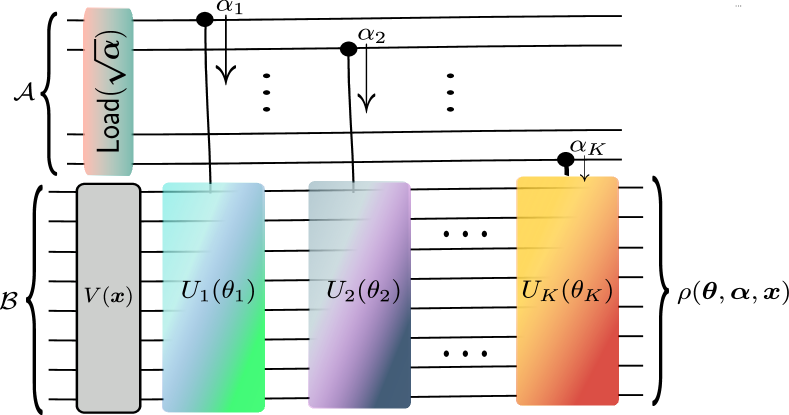
i

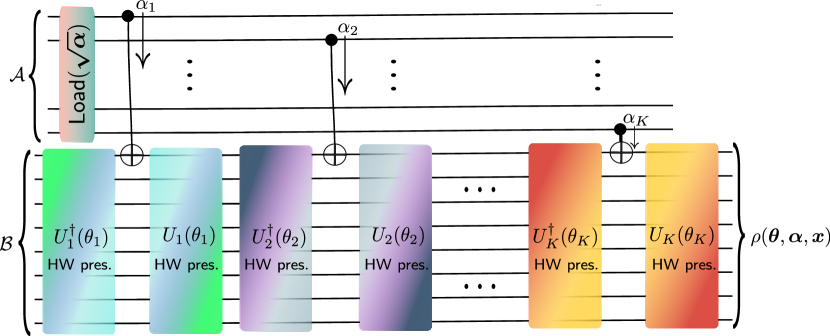
ii

Figure 9: Circuits for preparing density QNN state. 9i) for generic sub-unitaries $U_{k}$ with a data encoding unitary $V(\mathbf{x})$. 9ii) for Hamming-weight preserving unitaries, $U_{k}$, with a trivial input state. In both cases, we load the distribution $\alpha$ to register $\mathcal{A}$ using a state preparation or loader circuit, for example a vector loader [48, 12, 16] if $\boldsymbol{\alpha}$ is known. In general, this distribution may also be prepared and learned by a quantum circuit, or may also be data-dependent (an ‘attention’ mechanism) as we discuss in the main text. The unary nature of the state in $\mathcal{A}$ means each qubit, $k$, is exactly associated with a probability, $\alpha_{k}$. We can directly access this probability by controlling on the activated qubit, $k$ in the unary basis. For each $k$ we have a control to register $B$. In the generic case (9i) the sub-unitaries are directly controlled and only applied to the data register, $\mathcal{B}$, if the corresponding probability in $\mathcal{A}$ is non-zero. In the Hamming-weight or unary case (9ii) the density state can be prepared for generative purposes and we only interact the registers $\mathcal{A}$ and $\mathcal{B}$ using two qubit CNOT gates. In both cases, the circuit depth will be linear in $K$ since $\mathsf{Load}\left(\sqrt{\boldsymbol{\alpha}}\right)$ can be implemented in depth $\log(K)$ with a parallel vector loader [48]. However, the depth in $n$ depends on the sub-unitaries $\{U_{k}(\theta_{k})\}_{k}$, and the ease of controlling them. In (9ii) however the depth can be provably logarithmic in $n$ if, for example, trainable ‘loader’ circuits are used for the ansatz, $\{U_{k}(\theta_{k})\}_{k}$. This case corresponds exactly to loading a particular matrix and the circuit behaves as a matrix loader [16].

D.3   Evaluation circuit for Density QNNs

Here we describe how the matrix loader in Fig. 9 prepares the state eq. (27). The matrix loader was originally intended to load an $n\times d$ matrix, $\mathbf{X}$, into an overall Hamming-weight $2$ state using two unary qubit registers; one to index the matrix rows and the other to index the columns as follows: $\ket{\mathbf{X}}=\frac{1}{||\mathbf{X}||}\sum_{i=1}^{n}\sum_{j=1}^{d}\mathbf{X}_{i,j}\ket{\boldsymbol{e}_{i}}\ket{\boldsymbol{e}_{j}}$. Intuitively, this works by loading first the column indices to the top register. Controlled on these ‘row’ indices, ‘row’ loaders are applied (Figure 5 in [16]) to the qubits in the bottom register ($\mathcal{B}$) in the figure. Due to the unary encoding on the top register, each control will be only activated corresponding to the row that qubit is indexing.

We adapt this idea here to prepare the state $\rho(\boldsymbol{\theta},\boldsymbol{\alpha},\boldsymbol{x}))$. First, we load the distribution of sub-unitaries, $\{\alpha_{k}\}$ onto the top $K$ qubits. This produces the Hamming weight $1$ state in the register $\mathcal{A}$. We can simultaneously prepare the initial data state $\ket{\boldsymbol{x}}$ by applying $V(\boldsymbol{x})$ on the register $\mathcal{B}$:

$$\mathsf{Load}\left(\sqrt{\boldsymbol{\alpha}}\right)\ket{0}_{\mathcal{A}}^{\otimes n}V(\boldsymbol{x})\ket{0}_{\mathcal{B}}^{\otimes n}=\sum_{k=1}^{K}\sqrt{\alpha_{k}}\ket{\boldsymbol{e}_{k}}_{\mathcal{A}}\ket{\boldsymbol{x}}_{\mathcal{B}}$$ (28)

Now, iterating through the top $K$ qubits and applying $U_{k}(\theta_{k})$ on the register $\mathcal{B}$ controlled on qubit $k$ in register $\mathcal{A}$ results in:

$$\sum_{k=1}^{K}\sqrt{\alpha_{k}}\ket{\boldsymbol{e_{k}}}_{\mathcal{A}}\ket{\boldsymbol{x}}_{\mathcal{B}}\rightarrow \sum_{k=1}^{K}\sqrt{\alpha_{k}}\ket{\boldsymbol{e}_{k}}_{\mathcal{A}}U_{k}(\boldsymbol{\theta})\ket{\boldsymbol{x}}_{\mathcal{B}},$$ (29)

$$\implies \rho_{\mathcal{A}\mathcal{B}}=\sum_{k=1}^{K}\sum_{j=1}^{K}\sqrt{\alpha_{k}}\sqrt{\alpha_{j}}\outerproduct{\boldsymbol{e_{k}}}{\boldsymbol{e_{j}}}_{\mathcal{A}}\left[U_{k}(\boldsymbol{\theta})\outerproduct{\boldsymbol{x}}{\boldsymbol{x}}U^{\dagger}_{k}(\boldsymbol{\theta})\right]_{\mathcal{B}}$$ (30)

Finally, $\rho(\boldsymbol{\theta},\boldsymbol{\alpha},\boldsymbol{x})=\tr_{\mathcal{A}}\left(\rho_{\mathcal{A}\mathcal{B}}\right)$ in eq. (27) is prepared by tracing out register $\mathcal{A}$, leaving only the trace-full diagonal elements $\outerproduct{\boldsymbol{e}_{k}}{\boldsymbol{e}_{k}}$ with trace $=1$.

There are some final notes on this point:

1. This technique of applying controlled unitaries a circuit is well-known as the linear combination of unitaries (LCU) method, which is a primary method of performing quantum simulation on a quantum computer. The LCU method emulates the effect of a non-unitary matrix $A$ on a state which can be decomposed as a linear combination of unitary operations, $A=\sum_{i}\alpha_{i}U_{i}$. While this work was in preparation, we became aware of [61] which proposes exactly the LCU method for quantum machine learning. However, this differs from the proposal in this work as we are interested in trading off efficiency and trainability for already defined models.

2. Dealing with the density state as here means we do not require post selection on the top register, $\mathcal{A}$. Post-selecting on a particular outcome, e.g. $\ket{0}^{\otimes n}$ adds an addition overhead to the overall model, but is necessary for correctly applying the desired matrix, $A$, to the input.

3. If we need to reuse the ancillary qubits in register $\mathcal{A}$ for another purpose after the creation of the density state, we will need to uncompute the qubits with the operation $\mathsf{Load}^{\dagger}\left(\sqrt{\boldsymbol{\alpha}}\right)$.

D.4   Sampling from Density QNNs

If we have a case where there is no data to be encoded into the circuit, i.e. $V(\boldsymbol{x})=\mathds{1}$ and the sub-unitaries $\mathcal{U}=\{U_{k}\}_{k=1}^{K}$ are all Hamming-weight preserving, we can use a closer analogue to the matrix loader of [16] to prepare the state $\rho(\boldsymbol{\theta},\boldsymbol{\alpha})$ (notice $\boldsymbol{x}$ independence) as in Fig. 9ii. Instead of directly controlling on the unitaries $U_{k}$, we instead interleave a CNOT gate between the unitary and its inverse. Since $U_{k}$ is Hamming-weight preserving, it will be activated with probability $\alpha_{k}$ as before, but since the initial state is Hamming weight $0$, the inverses, $U^{\dagger}_{k}(\theta_{k})$, will not apply for that particular $k$, only the CNOT which activates an initial unary state followed by the unitary $U_{k}(\theta_{k})$, which preserves the Hamming-weight $1$ state on the $\mathcal{B}$ register. If these Hamming-weight preserving unitaries are vector loaders [16], the output state $\rho(\boldsymbol{\theta},\boldsymbol{\alpha})$ will correspond exactly the reduced state of some, unknown, matrix loader state $\ket{\mathbf{X}^{*}}$ generated by the angles $\boldsymbol{\theta}$:

$$\ket{\mathbf{X}^{*}} =\sum_{i=1}^{n}\sum_{k=1}^{d}\sqrt{\alpha_{k}}\mathbf{X}^{*}_{i,k}\ket{\boldsymbol{e}_{k}}_{\mathcal{A}}\ket{\boldsymbol{e}_{i}}_{\mathcal{B}}$$

$$\rho_{\mathcal{A}\mathcal{B}} =\sum_{i=1}^{n}\sum_{i^{\prime}=1}^{n}\sum_{k=1}^{d}\sum_{k^{\prime}=1}^{d}\sqrt{\alpha_{k}\alpha_{k^{\prime}}}\mathbf{X}^{*}_{i,k}\mathbf{X}^{*}_{i^{\prime},k^{\prime}}\outerproduct{\boldsymbol{e}_{k}}{\boldsymbol{e}_{k^{\prime}}}_{\mathcal{A}}\outerproduct{\boldsymbol{e}_{i}}{\boldsymbol{e}_{i}}_{\mathcal{B}}$$

$$\implies\rho(\boldsymbol{\theta},\boldsymbol{\alpha}) =\sum_{i=1}^{n}\sum_{i^{\prime}=1}^{n}\sum_{k=1}^{d}\alpha_{k}\mathbf{X}^{*}_{i,k}\mathbf{X}^{*}_{i^{\prime},k}\outerproduct{\boldsymbol{e}_{i}}{\boldsymbol{e}_{i^{\prime}}}_{\mathcal{B}}$$

Here, we can view the DenQNN as preparing a generative state (akin to a Born machine [62, 63, 64, 65]) and sampling the state in the computational basis can correspond to sampling an index $i\in[n]$ with probability weighted by $\sum_{k}\alpha_{k}^{2}\left(\mathbf{X}^{*}_{i,k}\right)^{2}$, where $\mathbf{X}^{*}_{*,k}$ is a vector (suitably normalised) derived from the angles $\boldsymbol{\theta}$. One could also generate a more efficient circuit in the unary space which includes an initial state preparation unitary using recent techniques from quantum fourier networks [66].

Here, we note the connection to the recently proposed variational measurement-based quantum computing (MBQC), which was applied to generative modelling [19]. There, a distribution over “sub-unitaries” appears naturally due the the nature of measurement-driven quantum computation. Specifically, each time a qubit is measured in the MBQC model, its output result is used to fork the next level of computation. In order to deterministically implement a single (yet arbitrary) unitary, MBQC corrects the ‘wrong’ path in the fork by applying corrective rotations on subsequent qubits. Rather than being motivated by implementing a single (known) unitary via deterministic correction, Ref. [19] proposes to use this inherent MBQC measurement randomness for generative modelling purposes, as the effect of not correcting outcomes results exactly in a mixed-unitary (density) channel as we have above. Similarly to our proposal, the authors demonstrated superior learning capabilities of the mixed channel over a single unitary ansatz. We hope that the parallel tracks traversed in our work, along with variational MBQC, and post-variational quantum machine learning can be unified to ultimately advance the field.

Appendix E Density reuploading quantum neural networks

A generalisation one can make for density quantum neural networks eq. (10) is when building classifiers or regressors, for classical data. Here, we can incorporate data reuploading [67, 68] in a natural way:

Definition 2 (Density QNNs with data reuploading).

Given a classical data point (vector or otherwise), $\boldsymbol{x}$, we can define a density QNN incorporating data reuploading as:

$$\rho^{R}(\boldsymbol{\theta},\boldsymbol{\alpha},\boldsymbol{x}) =\sum_{k=1}^{K}\alpha_{k}\mathcal{E}_{\boldsymbol{\theta},\boldsymbol{x}}^{R}(\outerproduct{0}{0}^{\otimes n})$$ (31)

$$\mathcal{E}^{R}_{\boldsymbol{\theta},\boldsymbol{x}}(\rho):=\underbrace{\mathcal{E}^{R}_{\boldsymbol{\theta}^{R},\boldsymbol{x}}\left(\cdots\mathcal{E}^{2}_{\boldsymbol{\theta}^{2},\boldsymbol{x}}\left(\mathcal{E}^{1}_{\boldsymbol{\theta}^{1},\boldsymbol{x}}(\rho)\right)\right)}_{R\ \textsf{times}}, \qquad\mathcal{E}^{r}_{\boldsymbol{\theta}^{r},\boldsymbol{x}}(\rho):=U_{k}(\boldsymbol{\theta}^{r}_{k})V(\boldsymbol{x})\rho V^{\dagger}(\boldsymbol{x})U^{\dagger}_{k}(\boldsymbol{\theta}^{r}_{k})$$ (32)

For two reuploads the density state is:

$$\rho^{2}(\boldsymbol{\theta},\boldsymbol{\alpha},\boldsymbol{x})=\sum_{k=1}^{K}\alpha_{k}U(\boldsymbol{\theta}^{2}_{k})V_{\boldsymbol{x}}U(\boldsymbol{\theta}^{1}_{k})\outerproduct{\boldsymbol{x}}{\boldsymbol{x}}U^{\dagger}(\boldsymbol{\theta}^{1}_{k})V_{\boldsymbol{x}}U^{\dagger}(\boldsymbol{\theta}^{2}_{k})$$ (33)

Where we drop the subscript $k$ on the sub-unitaries for compactness, and $V_{\boldsymbol{x}}:=V({\boldsymbol{x}})$. Now, in the case of sub-unitaries which are decomposed into (commuting-)blocks, somewhat confusingly, $\boldsymbol{\theta}$ is a rank $4$ tensor, $\boldsymbol{\theta}:=\{\theta^{r,b}_{k,j}\}$ where $r,b,k,j$ indexes the upload, block, sub-unitary and parameter respectively. Now unfortunately it is not clear in general how to efficiently train the above models in Definition 2 even if each unitary is of a commuting-block form of Ref. [15]. This is because the arbitrary nature of the data encoding unitary, $V(\boldsymbol{x})$ prohibits a fixed commutation relation between unitaries in subsequent uploads. However, there is one potential solution to this, which is to train in a layerwise fashion. For example, one first trains the first uploaded unitaries, $U(\boldsymbol{\theta}_{k}^{1})$. Then, defining $V^{\prime}_{\boldsymbol{x}}:=V_{\boldsymbol{x}}U(\boldsymbol{\theta}_{k}^{1})V_{\boldsymbol{x}}$ as the new (fixed) ‘encoding’ unitary, we train the next upload $U(\boldsymbol{\theta}_{k}^{2})$, and so in. So a scheme would allow gradient scaling with an additional factor of $\mathcal{O}(R)$ overhead to that of the single reuploading model,  Theorem 1. In the above, we assume that the unitaries applied are the same in successive reuploads - i.e. if the random variable we employ chooses sub-unitary, $U_{k}$, to apply to the initial state for the first upload, the subsequent sub-unitaries applied are also $U_{k}$, although with potentially different parameters, $\boldsymbol{\theta}_{k}^{1}\neq\boldsymbol{\theta}_{k}^{2}$. In this case the distribution $\{\alpha_{k}\}$ represents the distribution of reuploading ‘sequences’. One could also account for different distributions over each reupload. For example, we apply one upload to the state and get $U(\boldsymbol{\theta}^{1}_{k})\outerproduct{\boldsymbol{x}}{\boldsymbol{x}}U^{\dagger}(\boldsymbol{\theta}^{1}_{k})$ with probability $\alpha_{k}$. If we choose a different (but independent) distribution, $\{\beta_{k^{\prime}}\}$, to select $U(\boldsymbol{\theta}^{2}_{k^{\prime}})$, the resulting state would be $U(\boldsymbol{\theta}^{2}_{k^{\prime}})V_{\boldsymbol{x}}U(\boldsymbol{\theta}^{1}_{k})\outerproduct{\boldsymbol{x}}{\boldsymbol{x}}U^{\dagger}(\boldsymbol{\theta}^{1}_{k})V_{\boldsymbol{x}}U^{\dagger}(\boldsymbol{\theta}^{2}_{k^{\prime}})$ with probability $\alpha_{k}\beta_{k^{\prime}}$, and so on.

Appendix F Experiment details

F.1   Hyperparameter optimisation

For hyperparameter optimisation, we use the hyperparameter tuning package optuna [69].

For the experiments in the main text relating to OrthoQNNs and their density counterparts, we use the following choice of hyperparameters:

• $\texttt{batch\_size}\in\{32,48,64,80,\dots,256\}$

• $\texttt{learning\_rate}\in[1\times 10^{-4},1\times 10^{-2}]$

• $\texttt{optimiser}\in\{\texttt{Adam},\texttt{SGD},\texttt{RMSProp}\}$

• $\texttt{regularisation}\in\{\ell_{2},\texttt{None}\}$

The (initial) learning rate is sampled uniformly on a logarithmic scale, and the regularisation (either $\ell_{2}$ norm regularisation or no regularisation) is added to the loss function, which in all cases is the cross entropy loss between model outputs and the true labels. The specific plot (6ii) shows the average over the best $\frac{x}{32}$ hyperparameter runs, those which achieve at least $70\%$ accuracy during training. For each model we have 6ii i a) (OrthoQNN): $\frac{32}{32}$, 6ii i b) (Density OrthoQNN): $\frac{29}{32}$, 6ii i c) (Density OrthoQNN (compressed): $\frac{31}{32}$. Increasing the criterion to $90\%$ accuracy, the relative success drops to OrthoQNN: $\frac{26}{32}$, Density OrthoQNN: $\frac{20}{32}$, Density OrthoQNN (compressed): $\frac{22}{32}$ respectively.

References

- [1] D. E. Rumelhart, G. E. Hinton, and R. J. Williams, “Learning representations by back-propagating errors,” Nature, vol. 323, no. 6088, pp. 533–536, Oct. 1986. [Online]. Available: https://www.nature.com/articles/323533a0
- [2] M. Benedetti, E. Lloyd, S. Sack, and M. Fiorentini, “Parameterized quantum circuits as machine learning models,” Quantum Sci. Technol., vol. 4, no. 4, p. 043001, Nov. 2019. [Online]. Available: https://dx.doi.org/10.1088/2058-9565/ab4eb5
- [3] K. Bharti, A. Cervera-Lierta, T. H. Kyaw, T. Haug, S. Alperin-Lea, A. Anand, M. Degroote, H. Heimonen, J. S. Kottmann, T. Menke, W.-K. Mok, S. Sim, L.-C. Kwek, and A. Aspuru-Guzik, “Noisy intermediate-scale quantum algorithms,” Rev. Mod. Phys., vol. 94, no. 1, p. 015004, Feb. 2022. [Online]. Available: https://link.aps.org/doi/10.1103/RevModPhys.94.015004
- [4] M. Cerezo, A. Arrasmith, R. Babbush, S. C. Benjamin, S. Endo, K. Fujii, J. R. McClean, K. Mitarai, X. Yuan, L. Cincio, and P. J. Coles, “Variational quantum algorithms,” Nat Rev Phys, vol. 3, no. 9, pp. 625–644, Sep. 2021. [Online]. Available: https://www.nature.com/articles/s42254-021-00348-9
- [5] M. Cerezo, G. Verdon, H.-Y. Huang, L. Cincio, and P. J. Coles, “Challenges and opportunities in quantum machine learning,” Nat Comput Sci, vol. 2, no. 9, pp. 567–576, Sep. 2022. [Online]. Available: https://www.nature.com/articles/s43588-022-00311-3
- [6] K. Mitarai, M. Negoro, M. Kitagawa, and K. Fujii, “Quantum circuit learning,” Phys. Rev. A, vol. 98, no. 3, p. 032309, Sep. 2018. [Online]. Available: https://link.aps.org/doi/10.1103/PhysRevA.98.032309
- [7] G. E. Crooks, “Gradients of parameterized quantum gates using the parameter-shift rule and gate decomposition,” May 2019. [Online]. Available: http://arxiv.org/abs/1905.13311
- [8] J. G. Vidal and D. O. Theis, “Calculus on parameterized quantum circuits,” Dec. 2018. [Online]. Available: http://arxiv.org/abs/1812.06323
- [9] M. Schuld, V. Bergholm, C. Gogolin, J. Izaac, and N. Killoran, “Evaluating analytic gradients on quantum hardware,” Phys. Rev. A, vol. 99, no. 3, p. 032331, Mar. 2019. [Online]. Available: https://link.aps.org/doi/10.1103/PhysRevA.99.032331
- [10] R. Sweke, F. Wilde, J. Meyer, M. Schuld, P. K. Faehrmann, B. Meynard-Piganeau, and J. Eisert, “Stochastic gradient descent for hybrid quantum-classical optimization,” Quantum, vol. 4, p. 314, Aug. 2020. [Online]. Available: https://quantum-journal.org/papers/q-2020-08-31-314/
- [11] O. Kyriienko and V. E. Elfving, “Generalized quantum circuit differentiation rules,” Phys. Rev. A, vol. 104, no. 5, p. 052417, Nov. 2021. [Online]. Available: https://link.aps.org/doi/10.1103/PhysRevA.104.052417
- [12] J. Landman, N. Mathur, Y. Y. Li, M. Strahm, S. Kazdaghli, A. Prakash, and I. Kerenidis, “Quantum Methods for Neural Networks and Application to Medical Image Classification,” Quantum, vol. 6, p. 881, Dec. 2022. [Online]. Available: https://quantum-journal.org/papers/q-2022-12-22-881/
- [13] A. Abbas, R. King, H.-Y. Huang, W. J. Huggins, R. Movassagh, D. Gilboa, and J. R. McClean, “On quantum backpropagation, information reuse, and cheating measurement collapse,” arXiv.org, May 2023. [Online]. Available: https://arxiv.org/abs/2305.13362v1
- [14] A. Kandala, A. Mezzacapo, K. Temme, M. Takita, M. Brink, J. M. Chow, and J. M. Gambetta, “Hardware-efficient variational quantum eigensolver for small molecules and quantum magnets,” Nature, vol. 549, no. 7671, pp. 242–246, Sep. 2017. [Online]. Available: https://www.nature.com/articles/nature23879
- [15] J. Bowles, D. Wierichs, and C.-Y. Park, “Backpropagation scaling in parameterised quantum circuits,” Jun. 2023. [Online]. Available: http://arxiv.org/abs/2306.14962
- [16] E. A. Cherrat, I. Kerenidis, N. Mathur, J. Landman, M. Strahm, and Y. Y. Li, “Quantum Vision Transformers,” Sep. 2022. [Online]. Available: http://arxiv.org/abs/2209.08167
- [17] F. Hamze, “Parallelized Computation and Backpropagation Under Angle-Parametrized Orthogonal Matrices,” May 2021. [Online]. Available: http://arxiv.org/abs/2106.00003
- [18] P.-W. Huang and P. Rebentrost, “Post-variational quantum neural networks,” Jul. 2023. [Online]. Available: http://arxiv.org/abs/2307.10560
- [19] A. Majumder, M. Krumm, T. Radkohl, H. P. Nautrup, S. Jerbi, and H. J. Briegel, “Variational measurement-based quantum computation for generative modeling,” Oct. 2023. [Online]. Available: http://arxiv.org/abs/2310.13524
- [20] J. Bradbury, R. Frostig, P. Hawkins, M. J. Johnson, C. Leary, D. Maclaurin, G. Necula, A. Paszke, J. VanderPlas, S. Wanderman-Milne, and Q. Zhang, “JAX: composable transformations of Python+NumPy programs,” 2018. [Online]. Available: http://github.com/google/jax
- [21] A. Griewank, K. Kulshreshtha, and A. Walther, “On the numerical stability of algorithmic differentiation,” Computing, vol. 94, no. 2, pp. 125–149, Mar. 2012. [Online]. Available: https://doi.org/10.1007/s00607-011-0162-z
- [22] J. Schmidhuber, “Deep learning in neural networks: An overview,” Neural Networks, vol. 61, pp. 85–117, Jan. 2015. [Online]. Available: https://www.sciencedirect.com/science/article/pii/S0893608014002135
- [23] J. Li, X. Yang, X. Peng, and C.-P. Sun, “Hybrid Quantum-Classical Approach to Quantum Optimal Control,” Phys. Rev. Lett., vol. 118, no. 15, p. 150503, Apr. 2017. [Online]. Available: https://link.aps.org/doi/10.1103/PhysRevLett.118.150503
- [24] D. Wierichs, J. Izaac, C. Wang, and C. Y.-Y. Lin, “General parameter-shift rules for quantum gradients,” Quantum, vol. 6, p. 677, Mar. 2022. [Online]. Available: https://quantum-journal.org/papers/q-2022-03-30-677/
- [25] V. Bergholm, J. Izaac, M. Schuld, C. Gogolin, S. Ahmed, V. Ajith, M. S. Alam, G. Alonso-Linaje, B. AkashNarayanan, A. Asadi, J. M. Arrazola, U. Azad, S. Banning, C. Blank, T. R. Bromley, B. A. Cordier, J. Ceroni, A. Delgado, O. Di Matteo, A. Dusko, T. Garg, D. Guala, A. Hayes, R. Hill, A. Ijaz, T. Isacsson, D. Ittah, S. Jahangiri, P. Jain, E. Jiang, A. Khandelwal, K. Kottmann, R. A. Lang, C. Lee, T. Loke, A. Lowe, K. McKiernan, J. J. Meyer, J. A. Montañez-Barrera, R. Moyard, Z. Niu, L. J. O’Riordan, S. Oud, A. Panigrahi, C.-Y. Park, D. Polatajko, N. Quesada, C. Roberts, N. Sá, I. Schoch, B. Shi, S. Shu, S. Sim, A. Singh, I. Strandberg, J. Soni, A. Száva, S. Thabet, R. A. Vargas-Hernández, T. Vincent, N. Vitucci, M. Weber, D. Wierichs, R. Wiersema, M. Willmann, V. Wong, S. Zhang, and N. Killoran, “PennyLane: Automatic differentiation of hybrid quantum-classical computations,” Jul. 2022. [Online]. Available: http://arxiv.org/abs/1811.04968
- [26] M. Broughton, G. Verdon, T. McCourt, A. J. Martinez, J. H. Yoo, S. V. Isakov, P. Massey, R. Halavati, M. Y. Niu, A. Zlokapa, E. Peters, O. Lockwood, A. Skolik, S. Jerbi, V. Dunjko, M. Leib, M. Streif, D. Von Dollen, H. Chen, S. Cao, R. Wiersema, H.-Y. Huang, J. R. McClean, R. Babbush, S. Boixo, D. Bacon, A. K. Ho, H. Neven, and M. Mohseni, “TensorFlow Quantum: A Software Framework for Quantum Machine Learning,” Aug. 2021. [Online]. Available: http://arxiv.org/abs/2003.02989
- [27] X.-Z. Luo, J.-G. Liu, P. Zhang, and L. Wang, “Yao.jl: Extensible, Efficient Framework for Quantum Algorithm Design,” Quantum, vol. 4, p. 341, Oct. 2020. [Online]. Available: https://quantum-journal.org/papers/q-2020-10-11-341/
- [28] T. Jones and J. Gacon, “Efficient calculation of gradients in classical simulations of variational quantum algorithms,” Sep. 2020. [Online]. Available: http://arxiv.org/abs/2009.02823
- [29] E. A. Cherrat, S. Raj, I. Kerenidis, A. Shekhar, B. Wood, J. Dee, S. Chakrabarti, R. Chen, D. Herman, S. Hu, P. Minssen, R. Shaydulin, Y. Sun, R. Yalovetzky, and M. Pistoia, “Quantum Deep Hedging,” Quantum, vol. 7, p. 1191, Nov. 2023. [Online]. Available: https://quantum-journal.org/papers/q-2023-11-29-1191/
- [30] M. Cerezo, M. Larocca, D. García-Martín, N. L. Diaz, P. Braccia, E. Fontana, M. S. Rudolph, P. Bermejo, A. Ijaz, S. Thanasilp, E. R. Anschuetz, and Z. Holmes, “Does provable absence of barren plateaus imply classical simulability? Or, why we need to rethink variational quantum computing,” Mar. 2024. [Online]. Available: http://arxiv.org/abs/2312.09121
- [31] M. Larocca, P. Czarnik, K. Sharma, G. Muraleedharan, P. J. Coles, and M. Cerezo, “Diagnosing Barren Plateaus with Tools from Quantum Optimal Control,” Quantum, vol. 6, p. 824, Sep. 2022. [Online]. Available: https://quantum-journal.org/papers/q-2022-09-29-824/
- [32] L. Monbroussou, J. Landman, A. B. Grilo, R. Kukla, and E. Kashefi, “Trainability and Expressivity of Hamming-Weight Preserving Quantum Circuits for Machine Learning,” Sep. 2023. [Online]. Available: http://arxiv.org/abs/2309.15547
- [33] B. Kiani, R. Balestriero, Y. LeCun, and S. Lloyd, “projUNN: efficient method for training deep networks with unitary matrices,” Oct. 2022. [Online]. Available: http://arxiv.org/abs/2203.05483
- [34] H.-Y. Huang, K. Bharti, and P. Rebentrost, “Near-term quantum algorithms for linear systems of equations with regression loss functions,” New J. Phys., vol. 23, no. 11, p. 113021, Nov. 2021. [Online]. Available: https://dx.doi.org/10.1088/1367-2630/ac325f
- [35] S. Aaronson, “Shadow Tomography of Quantum States,” Nov. 2018. [Online]. Available: http://arxiv.org/abs/1711.01053
- [36] H.-Y. Huang, R. Kueng, and J. Preskill, “Predicting many properties of a quantum system from very few measurements,” Nat. Phys., vol. 16, no. 10, pp. 1050–1057, Oct. 2020. [Online]. Available: https://www.nature.com/articles/s41567-020-0932-7
- [37] I. Kerenidis and A. Prakash, “Quantum machine learning with subspace states,” Feb. 2022. [Online]. Available: http://arxiv.org/abs/2202.00054
- [38] N. Srivastava, G. Hinton, A. Krizhevsky, I. Sutskever, and R. Salakhutdinov, “Dropout: a simple way to prevent neural networks from overfitting,” J. Mach. Learn. Res., vol. 15, no. 1, pp. 1929–1958, Jan. 2014.
- [39] P. Baldi and P. J. Sadowski, “Understanding Dropout,” in Advances in Neural Information Processing Systems, C. J. Burges, L. Bottou, M. Welling, Z. Ghahramani, and K. Q. Weinberger, Eds., vol. 26. Curran Associates, Inc., 2013. [Online]. Available: https://proceedings.neurips.cc/paper_files/paper/2013/file/71f6278d140af599e06ad9bf1ba03cb0-Paper.pdf
- [40] Q. T. Nguyen, L. Schatzki, P. Braccia, M. Ragone, P. J. Coles, F. Sauvage, M. Larocca, and M. Cerezo, “Theory for Equivariant Quantum Neural Networks,” Oct. 2022. [Online]. Available: http://arxiv.org/abs/2210.08566
- [41] G. Verdon, J. Marks, S. Nanda, S. Leichenauer, and J. Hidary, “Quantum Hamiltonian-Based Models and the Variational Quantum Thermalizer Algorithm,” Oct. 2019. [Online]. Available: http://arxiv.org/abs/1910.02071
- [42] N. Ezzell, E. M. Ball, A. U. Siddiqui, M. M. Wilde, A. T. Sornborger, P. J. Coles, and Z. Holmes, “Quantum mixed state compiling,” Quantum Sci. Technol., vol. 8, no. 3, p. 035001, Apr. 2023. [Online]. Available: https://dx.doi.org/10.1088/2058-9565/acc4e3
- [43] G. Brassard, P. Hoyer, M. Mosca, and A. Tapp, “Quantum Amplitude Amplification and Estimation,” in Quantum Computation and Information, 2002, vol. 305, pp. 53–74. [Online]. Available: http://arxiv.org/abs/quant-ph/0005055
- [44] W. J. Huggins, K. Wan, J. McClean, T. E. O’Brien, N. Wiebe, and R. Babbush, “Nearly Optimal Quantum Algorithm for Estimating Multiple Expectation Values,” Phys. Rev. Lett., vol. 129, no. 24, p. 240501, Dec. 2022. [Online]. Available: https://link.aps.org/doi/10.1103/PhysRevLett.129.240501
- [45] J. R. McClean, S. Boixo, V. N. Smelyanskiy, R. Babbush, and H. Neven, “Barren plateaus in quantum neural network training landscapes,” Nat Commun, vol. 9, no. 1, p. 4812, Nov. 2018. [Online]. Available: https://www.nature.com/articles/s41467-018-07090-4
- [46] I. Cong, S. Choi, and M. D. Lukin, “Quantum convolutional neural networks,” Nat. Phys., vol. 15, no. 12, pp. 1273–1278, Dec. 2019. [Online]. Available: https://www.nature.com/articles/s41567-019-0648-8
- [47] J. Bowles, “josephbowles/backprop_scaling,” Jun. 2023. [Online]. Available: https://github.com/josephbowles/backprop_scaling
- [48] S. Johri, S. Debnath, A. Mocherla, A. Singk, A. Prakash, J. Kim, and I. Kerenidis, “Nearest centroid classification on a trapped ion quantum computer,” npj Quantum Inf, vol. 7, no. 1, pp. 1–11, Aug. 2021. [Online]. Available: https://www.nature.com/articles/s41534-021-00456-5
- [49] D. Bahdanau, K. Cho, and Y. Bengio, “Neural Machine Translation by Jointly Learning to Align and Translate,” May 2016. [Online]. Available: http://arxiv.org/abs/1409.0473
- [50] I. Sutskever, O. Vinyals, and Q. V. Le, “Sequence to Sequence Learning with Neural Networks,” in Advances in Neural Information Processing Systems, Z. Ghahramani, M. Welling, C. Cortes, N. Lawrence, and K. Q. Weinberger, Eds., vol. 27. Curran Associates, Inc., 2014. [Online]. Available: https://proceedings.neurips.cc/paper_files/paper/2014/file/a14ac55a4f27472c5d894ec1c3c743d2-Paper.pdf
- [51] A. Vaswani, N. Shazeer, N. Parmar, J. Uszkoreit, L. Jones, A. N. Gomez, L. Kaiser, and I. Polosukhin, “Attention is All you Need,” in Advances in Neural Information Processing Systems, I. Guyon, U. V. Luxburg, S. Bengio, H. Wallach, R. Fergus, S. Vishwanathan, and R. Garnett, Eds., vol. 30. Curran Associates, Inc., 2017. [Online]. Available: https://proceedings.neurips.cc/paper_files/paper/2017/file/3f5ee243547dee91fbd053c1c4a845aa-Paper.pdf
- [52] D. T. Tran, J. Kanniainen, M. Gabbouj, and A. Iosifidis, “Data Normalization for Bilinear Structures in High-Frequency Financial Time-series,” in 2020 25th International Conference on Pattern Recognition (ICPR). Milan, Italy: IEEE, Jan. 2021, pp. 7287–7292. [Online]. Available: https://ieeexplore.ieee.org/document/9412547/
- [53] G. Verdon, M. Broughton, J. R. McClean, K. J. Sung, R. Babbush, Z. Jiang, H. Neven, and M. Mohseni, “Learning to learn with quantum neural networks via classical neural networks,” Jul. 2019. [Online]. Available: http://arxiv.org/abs/1907.05415
- [54] M. Wilson, R. Stromswold, F. Wudarski, S. Hadfield, N. M. Tubman, and E. G. Rieffel, “Optimizing quantum heuristics with meta-learning,” Quantum Mach. Intell., vol. 3, no. 1, p. 13, Apr. 2021. [Online]. Available: https://doi.org/10.1007/s42484-020-00022-w
- [55] G.-L. R. Anselmetti, D. Wierichs, C. Gogolin, and R. M. Parrish, “Local, expressive, quantum-number-preserving VQE ansätze for fermionic systems,” New J. Phys., vol. 23, no. 11, p. 113010, Nov. 2021. [Online]. Available: https://dx.doi.org/10.1088/1367-2630/ac2cb3
- [56] S. Kazdaghli, I. Kerenidis, J. Kieckbusch, and P. Teare, “Improved clinical data imputation via classical and quantum determinantal point processes,” Dec. 2023. [Online]. Available: http://arxiv.org/abs/2303.17893
- [57] S. Thakkar, S. Kazdaghli, N. Mathur, I. Kerenidis, A. J. Ferreira-Martins, and S. Brito, “Improved Financial Forecasting via Quantum Machine Learning,” Apr. 2024. [Online]. Available: http://arxiv.org/abs/2306.12965
- [58] I. Kerenidis, J. Landman, and A. Prakash, “Quantum Algorithms for Deep Convolutional Neural Networks,” in International Conference on Learning Representations, 2020. [Online]. Available: http://arxiv.org/abs/1911.01117
- [59] F. Scala, A. Ceschini, M. Panella, and D. Gerace, “A General Approach to Dropout in Quantum Neural Networks,” Adv Quantum Tech, p. 2300220, Dec. 2023. [Online]. Available: http://arxiv.org/abs/2310.04120
- [60] M. Kobayashi, K. Nakaji, and N. Yamamoto, “Overfitting in quantum machine learning and entangling dropout,” Quantum Mach. Intell., vol. 4, no. 2, p. 30, Nov. 2022. [Online]. Available: https://doi.org/10.1007/s42484-022-00087-9
- [61] J. Heredge, M. West, L. Hollenberg, and M. Sevior, “Non-Unitary Quantum Machine Learning,” May 2024. [Online]. Available: http://arxiv.org/abs/2405.17388
- [62] S. Cheng, J. Chen, and L. Wang, “Information Perspective to Probabilistic Modeling: Boltzmann Machines versus Born Machines,” Entropy, vol. 20, no. 8, p. 583, Aug. 2018. [Online]. Available: https://www.mdpi.com/1099-4300/20/8/583
- [63] J.-G. Liu and L. Wang, “Differentiable learning of quantum circuit Born machines,” Phys. Rev. A, vol. 98, no. 6, p. 062324, Dec. 2018. [Online]. Available: https://link.aps.org/doi/10.1103/PhysRevA.98.062324
- [64] M. Benedetti, D. Garcia-Pintos, O. Perdomo, V. Leyton-Ortega, Y. Nam, and A. Perdomo-Ortiz, “A generative modeling approach for benchmarking and training shallow quantum circuits,” npj Quantum Inf, vol. 5, no. 1, pp. 1–9, May 2019. [Online]. Available: https://www.nature.com/articles/s41534-019-0157-8
- [65] B. Coyle, D. Mills, V. Danos, and E. Kashefi, “The Born supremacy: quantum advantage and training of an Ising Born machine,” npj Quantum Inf, vol. 6, no. 1, pp. 1–11, Jul. 2020, publisher: Nature Publishing Group. [Online]. Available: https://www.nature.com/articles/s41534-020-00288-9
- [66] N. Jain, J. Landman, N. Mathur, and I. Kerenidis, “Quantum Fourier networks for solving parametric PDEs,” Quantum Sci. Technol., vol. 9, no. 3, p. 035026, May 2024, publisher: IOP Publishing. [Online]. Available: https://dx.doi.org/10.1088/2058-9565/ad42ce
- [67] A. Pérez-Salinas, A. Cervera-Lierta, E. Gil-Fuster, and J. I. Latorre, “Data re-uploading for a universal quantum classifier,” Quantum, vol. 4, p. 226, Feb. 2020. [Online]. Available: https://quantum-journal.org/papers/q-2020-02-06-226/
- [68] M. Schuld, R. Sweke, and J. J. Meyer, “Effect of data encoding on the expressive power of variational quantum-machine-learning models,” Phys. Rev. A, vol. 103, no. 3, p. 032430, Mar. 2021. [Online]. Available: https://link.aps.org/doi/10.1103/PhysRevA.103.032430
- [69] T. Akiba, S. Sano, T. Yanase, T. Ohta, and M. Koyama, “Optuna: A Next-Generation Hyperparameter Optimization Framework,” in The 25th ACM SIGKDD International Conference on Knowledge Discovery & Data Mining, 2019, pp. 2623–2631.