The Empirical Impact of Neural Parameter Symmetries, or Lack Thereof

Abstract

Many algorithms and observed phenomena in deep learning appear to be affected by parameter symmetries — transformations of neural network parameters that do not change the underlying neural network function. These include linear mode connectivity, model merging, Bayesian neural network inference, metanetworks, and several other characteristics of optimization or loss-landscapes. However, theoretical analysis of the relationship between parameter space symmetries and these phenomena is difficult. In this work, we empirically investigate the impact of neural parameter symmetries by introducing new neural network architectures that have reduced parameter space symmetries. We develop two methods, with some provable guarantees, of modifying standard neural networks to reduce parameter space symmetries. With these new methods, we conduct a comprehensive experimental study consisting of multiple tasks aimed at assessing the effect of removing parameter symmetries. Our experiments reveal several interesting observations on the empirical impact of parameter symmetries; for instance, we observe linear mode connectivity between our networks without alignment of weight spaces, and we find that our networks allow for faster and more effective Bayesian neural network training.

1 Introduction

Neural networks have found profound empirical success, but have many associated behaviors and phenomena that are difficult to understand. One important property of neural networks is that they generally have many parameter space symmetries — for any set of parameters, there are typically many other choices of parameters that correspond to the same exact neural network function [23]. For instance, permutations of hidden neurons in a multi-layer perceptron (MLP) induce permutations of weights that leave the overall input-output relationship unchanged. These parameter symmetries are a type of (not-necessarily detrimental) redundancy in the parameterization of neural networks, that adds much non-Euclidean structure to parameter space.

Parameter space symmetries appear to influence several phenomena observed in neural networks. For example, when linearly interpolating between the parameters of two independently trained networks with the same architecture, the intermediate networks typically perform poorly [57, 12]. However, if we first align the two networks via a permutation of parameters that does not affect the network function, then the intermediate networks can perform just as well as the unmerged networks [57, 1]. In some sense, this suggests that neural network loss landscapes are more convex or well-behaved after removing permutation symmetries. Other areas that parameter symmetries play a role in include interpretability of neurons [19], optimization [46, 80, 76], model merging [58], learned equivariance [6], Bayesian deep learning [33], loss landscape geometry [52], processing neural network weights as input data using metanetworks [38], and generalization measures [47, 10].

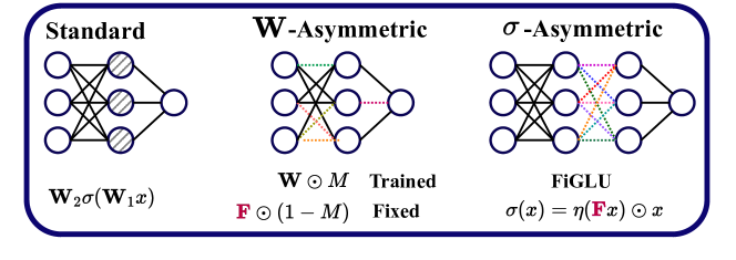
Figure 1: (Left) Standard MLP. The hidden nodes (grey hatches) can be freely permuted, which induces permutation parameter symmetries. Black edges denote trainable parameters. (Middle) Our $\mathbf{W}$-Asymmetric MLP, which fixes certain weights to be constant and untrainable (colored dashed lines) to break parameter symmetries. (Right) Our $\sigma$-Asymmetric MLP, which uses our FiGLU nonlinearity involving a fixed matrix $\mathbf{{\color[rgb]{.75,0,.25}F}}$ (colored dashed lines) to break parameter symmetries.

To rigorously study the effect of parameter symmetries, we study the effect of removing them. In particular, we introduce two ways of modifying neural network architectures to remove parameter space symmetries (see Figure 1):

• $\mathbf{W}$-Asymmetric networks fix certain elements of each linear map to break symmetries in the computation graph.

• $\sigma$-Asymmetric networks use a new nonlinearity (FiGLU) that does not act elementwise, and hence does not induce symmetries such as permutations.

These two approaches are inspired by previous work, which shows that both symmetries of computation graphs [38] and equivariances of nonlinearities [19] induce parameter symmetries in standard neural networks. We theoretically prove that both of our approaches remove parameter symmetries under certain conditions. Our Asymmetric networks are similar structurally to standard networks and can be trained with standard backpropagation and first-order optimization algorithms like Adam. Thus, they are a reasonable “counterfactual” system for studying neural networks without parameter symmetries.

With our Asymmetric networks, we run a suite of experiments to study the effects of removing parameter symmetries on several base architectures, including MLPs, ResNets, and graph neural networks. We investigate linear mode connectivity, Bayesian deep learning, metanetworks, and monotonic linear interpolation. Through the lenses of linear mode connectivity and monotonic linear interpolation, we see that the loss landscapes of our Asymmetric networks are remarkably more well-behaved and closer to convex than the loss landscapes of standard neural networks. When using our Asymmetric networks as the base model in a Bayesian neural network, we find faster training and better performance than using standard neural networks that have many parameter symmetries. When using metanetworks to predict properties such as test accuracy of an input neural network, we see that all tested metanetworks more accurately predict the accuracy of Asymmetric networks than standard networks. Overall, our Asymmetric networks provide valuable insights for empirical study and hold promise for advancing our understanding of the impact of neural parameter symmetries.

2 Background and Definitions

Let $\Theta$ be the space of parameters of a fixed neural network architecture. For any choice of parameters $\theta\in\Theta$, we have a neural network function $f_{\theta}\mathrel{\mathop{\mathchar 58\relax}}\mathcal{X}\to\mathcal{Y}$ from an input space $\mathcal{X}$ to an output space $\mathcal{Y}$. We call a function $\phi\mathrel{\mathop{\mathchar 58\relax}}\Theta\to\Theta$ a parameter space symmetry if $f_{\theta}(x)=f_{\phi(\theta)}(x)$ for all inputs $x$ and parameters $\theta\in\Theta$ (i.e. if $f_{\theta}$ and $f_{\phi(\theta)}$ are always the same function).

For instance, consider a two-layer MLP with no biases, parameterized by matrices $\theta=(\mathbf{W}_{2},\mathbf{W}_{1})$ with an elementwise nonlinearity $\sigma$. Then $f_{\theta}(x)=\mathbf{W}_{2}\sigma(\mathbf{W}_{1}x)$. Let $P$ be a permutation matrix, and let $\phi(\theta)=(\mathbf{W}_{2}P^{\top},P\mathbf{W}_{1})$. Then for any input $x$,

$$f_{\phi(\theta)}(x)=\mathbf{W}_{2}P^{\top}\sigma(P\mathbf{W}_{1}x)=\mathbf{W}_{2}P^{\top}P\sigma(\mathbf{W}_{1}x)=\mathbf{W}_{2}\sigma(\mathbf{W}_{1}x)=f_{\theta}(x),$$ (1)

so $\phi$ is a parameter space symmetry. A key step is the second equality, which holds because $P\sigma(x)=\sigma(Px)$: any elementwise nonlinearity $\sigma$ is permutation equivariant. Any other equivariance of $\sigma$ also induces a parameter symmetry; for instance, if $\sigma(x)=\max(0,x)$ is the ReLU function, then $\alpha\sigma(x)=\sigma(\alpha x)$ for any $\alpha>0$, so there is a positive-scaling-based parameter symmetry [47, 10, 19].

3 Related Work

Characterizing parameter space symmetries. While many works spanning several decades have noted specific parameter space symmetries in neural networks [23, 59], some works take a more systematic approach to deriving parameter space symmetries. Godfrey et al. [19] characterize all global linear symmetries induced by the nonlinearity for two-layer multi-layer perceptrons with pointwise nonlinearities. Zhao et al. [74] study several types of symmetries, and derive nonlinear, data-dependent parameter space symmetries. Lim et al. [38] show that graph automorphisms of the computation graph of a neural network induce permutation parameter symmetries, which captures hidden neuron permutations in MLPs and hidden channel permutations in CNNs.

Constraints and post-processing to break parameter space symmetries. Several works develop methods for constraining or post-processing the weights of a single neural network to remove ambiguities from parameter space symmetries. This includes methods to remove scaling symmetries induced by normalization layers or positively-homogeneous nonlinearities such as $\mathrm{ReLU}$ [5, 53, 52, 35], methods to remove permutation symmetries [53, 52, 69, 35], and methods to remove sign symmetries induced by odd activation functions [69]. Unlike these previous works, we develop neural network architectures that have reduced parameter space symmetries. Our models are optimized using standard unconstrained gradient-descent based methods like Adam. Hence, our networks do not require any non-standard optimization algorithms such as manifold optimization or projected gradient descent [5, 53], nor do they require post-training-processing to remove symmetries or special care during analysis of parameters (such as geodesic interpolation in a Riemannian weight space [52]).

Aligning multiple networks for relative invariance to parameter symmetries. One way to reduce the impact of parameter symmetries in certain settings, especially for model merging, is to align the parameters of one network to another. Several methods have been proposed for choosing permutations that align the parameters of two neural networks of the same architecture, via efficient heuristics or learned methods [3, 67, 61, 12, 1, 51, 45, 65]. Other approaches relax the exact permutation-parameter-symmetry constraint or do additional postprocessing to achieve effective merging of models in parameter space [57, 27, 28, 58, 54]. As our Asymmetric networks have removed parameter symmetries, they can often be successfully merged and linearly interpolated between without any alignment.

4 Asymmetric Networks

We develop two methods of parameterizing neural network architectures without parameter symmetries, both of which are justified by theoretical results. We first focus on the case of fully-connected MLPs with no biases, which take the form $f_{\theta}(x)=\mathbf{W}_{L}\sigma(\mathbf{W}_{L-1}\cdots\sigma(\mathbf{W}_{1}x))$ for weights $\theta=(\mathbf{W}_{L},\ldots,\mathbf{W}_{1})$ and nonlinearity $\sigma$. Then in Section 4.3, we discuss how we use these approaches to remove parameter symmetries in other architectures as well.

4.1 Computation Graph Approach ($\mathbf{W}$-Asymmetric Networks)

Our first approach to developing neural networks with greatly reduced parameter space symmetries relies on their computation graph. In particular, we can write a feedforward neural network architecture as a DAG $G=(V,E)$ with neurons as nodes $V$ and connections between them as edges $E$. For a choice of parameters $\theta\in\mathbb{R}^{|E|}$, we get a function $f_{\theta}$ from input neuron space to output neuron space [18, 47, 38]

Lim et al. [38] showed that neural DAG automorphisms $\phi$, which are graph automorphisms of the DAG $G$ that preserve types of nodes and weight-sharing constraints, induce permutation parameter symmetries $\phi$ that leave the function unchanged: $f_{\theta}=f_{\phi(\theta)}$. Thus, any feedforward neural network architecture that has no permutation parameter symmetries must necessarily have a computation graph with no nontrivial neural DAG automorphisms.

To modify MLPs so they have no nontrivial neural DAG automorphisms, we mask edges in the computation graph, by setting certain edge weights to constant values that are not updated during training. For an MLP, we can do this by enforcing that every linear layer $T\mathrel{\mathop{\mathchar 58\relax}}\mathbb{R}^{d_{1}}\to\mathbb{R}^{d_{2}}$ takes the form of a matrix $\mathbf{W}\in\mathbb{R}^{d_{2}\times d_{1}}$, where each row has a unique pattern of untrained weights. To achieve this, define a mask $M\in\{0,1\}^{d_{2}\times d_{1}}$ such that $\mathbf{W}_{ij}$ is a trainable parameter if and only if $M_{ij}=1$, and the rows of $M$ are pairwise distinct binary vectors in $\{0,1\}^{d_{1}}$. We call any neural network with linear maps masked as such a $\mathbf{W}$-Asymmetric neural network. In Appendix B.1, we show that masking these entries so that they are not trained is sufficient to remove all nontrivial neural DAG automorphisms.

Theorem 1.

If each mask matrix $M$ has unique nonzero rows, then $\mathbf{W}$-Asymmetric MLPs with fixed entries set to zero have no nontrivial neural DAG automorphisms.

In practice, we generate a binary mask $M$ by randomly selecting a subset of $n_{\mathrm{fix}}$ fixed elements for each row. For the fixed entries, we sample them from a normal distribution $\mathcal{N}(0,\kappa I)$ with standard deviation $\kappa>0$ that we tune. Our asymmetric linear layer can be written as

$$\mathbf{W}^{\prime}=M\odot\mathbf{W}+(1-M)\odot\mathbf{{\color[rgb]{.75,0,.25}F}},$$ (2)

where $\mathbf{W}\in\mathbb{R}^{d_{2}\times d_{1}}$ is a matrix of trainable parameters, and $\mathbf{{\color[rgb]{.75,0,.25}F}}\in\mathbb{R}^{d_{2}\times d_{1}}$ is a matrix of fixed elements, sampled from $\mathcal{N}(0,\kappa I)$. The only trainable parameters are the unmasked entries of $M\odot\mathbf{W}$, of which there are $d_{2}\cdot(d_{1}-n_{\mathrm{fix}})$. We empirically find that having $\kappa$ be significantly larger than the standard deviation of typical initializations for weight matrices (e.g. $\kappa=1$ while the trained coefficients have standard deviation about $1/\sqrt{1000}$) is important for breaking parameter symmetries.

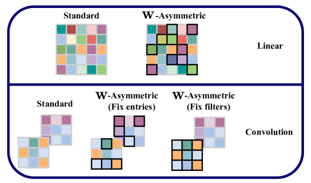
Figure 2: Depiction of our $\mathbf{W}$-Asymmetric approach to removing parameter symmetries. Entries with a black outline are untrained. Note that the $\mathbf{W}$-Asym linear map has 2 nonzeros per row, the $\mathbf{W}$-Asym convolution with fixed entries has 8 fixed entries for its single output channel, and the $\mathbf{W}$-Asym convolution with fixed filters has a single input filter fixed. We often use a constant number of fixed entries per row or output channel in our experiments.

4.2 Nonlinearity Approach ($\sigma$-Asymmetric Networks)

Another approach for removing parameter symmetries is to change the nonlinearity. As studied by Godfrey et al. [19], equivariances of the nonlinearity induce parameter symmetries in MLPs with elementwise nonlinearities. Recall that an elementwise nonlinearity acts by using the same function on each coordinate of the input; $\sigma\mathrel{\mathop{\mathchar 58\relax}}\mathbb{R}^{d}\to\mathbb{R}^{d}$ is elementwise if it takes the form $\sigma(x)=(\sigma_{1}(x_{1}),\ldots,\sigma_{1}(x_{d}))$ for some real function $\sigma_{1}\mathrel{\mathop{\mathchar 58\relax}}\mathbb{R}\to\mathbb{R}$. Any elementwise nonlinearity is permutation equivariant, and hence induces a permutation parameter symmetry.

Thus, in contrast to most neural network architectures, for Asymmetric networks we must use a nonlinearity that does not act elementwise. Likewise, the nonlinearity cannot have any linear symmetry itself, since if $\sigma\circ A=B\circ\sigma$ for $A,B\in GL(d)$, then for a two-layer network:

$$\mathbf{W}_{2}\circ\sigma\circ\mathbf{W}_{1}=\mathbf{W}_{2}B^{-1}B\circ\sigma\circ\mathbf{W}_{1}=\mathbf{W}_{2}B^{-1}\circ\sigma\circ A\mathbf{W}_{1}.$$ (3)

So $(\mathbf{W}_{2},\mathbf{W}_{1})$ and $(\mathbf{W}_{2}B^{-1},A\mathbf{W}_{1})$ give the same neural network function. Thus, in order to define a model class without parameter symmetries, it is necessary for $\sigma$ to have no linear equivariances, i.e. we desire that if $\sigma\circ A=B\circ\sigma$ for $A,B\in GL(d)$, then $A=B=I$. For two-layer MLPs with square invertible weights, this is in fact sufficient to remove all parameter symmetries: we prove this in Appendix B.2.

Proposition 1.

Let the parameter space $\Theta$ be all pairs of square invertible matrices $\theta=(\mathbf{W}_{2},\mathbf{W}_{1})$ for $\mathbf{W}_{2},\mathbf{W}_{1}\in GL(d)$, and let $f_{\theta}(x)=\mathbf{W}_{2}\sigma(\mathbf{W}_{1}x)$. If $\sigma$ has no linear equivariances, then $f_{\theta_{1}}=f_{\theta_{2}}$ if and only if $\theta_{1}=\theta_{2}$. In other words, there are no nontrivial parameter space symmetries.

4.2.1 FiGLU: the Fixed Gated Linear Unit Nonlinearity

Motivated by Proposition 1, we define a non-elementwise nonlinearity that does not have the equivariances of standard nonlinearities. Letting $\eta$ be the sigmoid function $\eta(x)=\frac{1}{1+e^{-x}}$, we define our nonlinearity as

$$\sigma(x)=\eta(\mathbf{{\color[rgb]{.75,0,.25}F}}x)\odot x,$$ (4)

for a randomly sampled, untrained matrix $\mathbf{{\color[rgb]{.75,0,.25}F}}$. In this work, we sample $\mathbf{{\color[rgb]{.75,0,.25}F}}$ as an i.i.d Gaussian matrix with variance that we tune. This nonlinearity is similar to Swish / SiLU [55, 25] with an additional matrix $\mathbf{{\color[rgb]{.75,0,.25}F}}$ to mix feature dimensions (to break permutation equivariance), and it is also similar to a gated linear unit (GLU) with no trainable parameters [8]. Thus, we call our nonlinearity FiGLU: the Fixed Gated Linear Unit.

In Appendix B.2.1, we prove that FiGLU does not have permutation equivariances or diagonal equivariances, which are the only equivariances for most elementwise nonlinearities [19].

Proposition 2.

With probability $1$ over the sampling of $\mathbf{{\color[rgb]{.75,0,.25}F}}$, FiGLU has no permutation equivariances or diagonal equivariances.

We call any network with our symmetry-breaking FiGLU nonlinearity a $\sigma$-Asymmetric Network.

4.3 Extension to Other Architectures

The graph-based approach ($\mathbf{W}$-Asymmetric Networks) works naturally for neural network architectures with “channel” dimensions, such as convolutional neural networks (CNNs), graph neural networks (GNNs) [21], Transformers [64], and equivariant neural networks based on equivariant linear maps [15]. In these types of networks, permutations of entire channels induce permutation parameter symmetries [38]. For such networks, we thus mask entire connections between channels, e.g. entire filters in CNNs. For CNNs, we also experiment with randomly masking some number of entries in each filter (instead of masking entire filters), and find that this also works well in removing parameter symmetries. For neural networks with linear layers that include bias terms, we do not modify the biases in any way, as they do not introduce new computation graph automorphisms [38].

The nonlinearity-based approach ($\sigma$-Asymmetric Networks) can be straightforwardly applied to many general architectures as well. Though, the fixed matrix $\mathbf{{\color[rgb]{.75,0,.25}F}}$ may have to be changed to a structured linear map; for instance, in CNNs we take $\mathbf{{\color[rgb]{.75,0,.25}F}}$ to be a 1D convolution.

4.4 Universal Approximation

Our two approaches remove parameter symmetries from standard neural networks, but still intuitively retain much of the structure of standard networks. One important property of widely-used neural network architectures is universal approximation — for any target function of a certain type, there exists a neural network of the given architecture that approximates the target to an arbitrary accuracy [7, 24, 41, 72]. In Appendix B.3, we show that $\mathbf{W}$-Asymmetric MLPs retain this property:

Theorem 2 (Informal).

For $n_{\mathrm{fix}}\in o(n^{\frac{1}{4}})$, where $n$ is the hidden dimension, $\mathbf{W}$-Asymmetric MLPs are Universal Approximators with probability $1$ over the choice of hardwired entries.

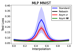
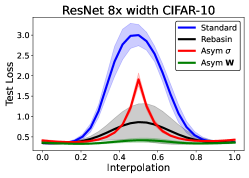
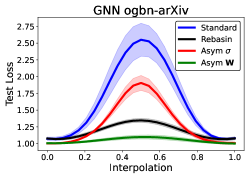
Figure 3: Linear mode connectivity: test loss curves along linear interpolations between trained networks. (Left) MLP on MNIST. (Middle) ResNet with $8\times$ width on CIFAR-10. (Right) GNN on ogbn-arXiv. $\mathbf{W}$-Asymmetric networks interpolate the best, followed by networks aligned with Git-Rebasin, then $\sigma$-Asymmetric networks, and finally standard networks.

5 Experiments

5.1 Linear Mode Connectivity without Permutation Alignment

Background. Many works have studied linear mode connectivity, which is when all networks on the line segment in parameter space between two well-performing trained networks are also well-performing [17, 42, 12]. When the two networks are randomly initialized and trained independently, linear mode connectivity generally does not hold [12, 1]. However, if one of the two networks is permuted with a parameter symmetry that does not change its function, but that aligns its parameters with the other network, then linear mode connectivity empirically and theoretically holds for many more model / task combinations [12, 1, 75, 13]. In fact, Entezari et al. [12] conjectures that if all permutation symmetries are accounted for, then linear mode connectivity generally holds. Since our Asymmetric networks remove parameter space symmetries, we may expect linear mode connectivity to hold, without any post-processing or alignment step.

Hypothesis. Asymmetric networks are more linearly mode connected than standard networks, and do not require post-processing or alignment of pairs of networks before merging.

Experimental Setup. We consider several networks and tasks: MLPs on MNIST, ResNets [22] on CIFAR-10, and Graph Neural Networks [71] on ogbn-arXiv [26]. For each architecture and task, we compute the midpoint test loss barrier: $L(\frac{1}{2}\theta_{1}+\frac{1}{2}\theta_{2})-\frac{1}{2}(L(\theta_{1})+L(\theta_{2}))$. This measures how much worse the interpolated network with parameters $\frac{1}{2}\theta_{1}+\frac{1}{2}\theta_{2}$ is than the original networks with parameters $\theta_{1}$ and $\theta_{2}$. We measure this barrier for standard networks, pairs of networks aligned with Git-Rebasin [1], and networks with our two approaches ($\sigma$-Asym and $\mathbf{W}$-Asym) applied.

Results. Figure 3 plots interpolation curves and Table 1 displays midpoint test loss barriers of various methods. Our $\sigma$-Asymmetric approach lowers the test loss barrier compared to standard networks, but falls short of the alignment approach of Git-Rebasin. On the other hand, our $\mathbf{W}$-Asymmetric approach achieves strong (and sometimes perfect) interpolation, and interpolates better than standard networks aligned via Git-ReBasin. This may be caused by failure of the Git-ReBasin approaches to find the optimal permutations, importance of other parameter symmetries besides layer-wise permutations, or other properties of $\mathbf{W}$-Asymmetric networks.

Table 1: Test loss interpolation barriers at midpoint: $L(\frac{1}{2}\theta_{1}+\frac{1}{2}\theta_{2})-\frac{1}{2}(L(\theta_{1})+L(\theta_{2}))$ . We use different methods of breaking symmetries in each column; from left to right: no symmetry breaking, Git-Rebasin [1], our $\sigma$-Asym approach, and our $\mathbf{W}$-Asym approach. We report mean and standard deviation of the barrier across at least 5 pairs of networks, and bold lowest barriers.

	Standard	Git-ReBasin	$\sigma$-Asym (ours)	$\mathbf{W}$-Asym (ours)
MLP (MNIST)	$0.188\pm.12$	$-.006\pm.00$	$0.117\pm.01$	$\mathbf{-0.012}\pm.00$
ResNet (CIFAR-10)	$3.287\pm.32$	$2.041\pm.21$	$2.521\pm.46$	$\mathbf{0.934}\pm.72$
ResNet 8x width (CIFAR-10)	$2.640\pm.24$	$0.509\pm.45$	$1.492\pm.15$	$\mathbf{0.031}\pm.05$
GNN (ogbn-arXiv)	$1.475\pm.24$	$0.269\pm.02$	$0.901\pm.11$	$\mathbf{0.095}\pm.03$

5.2 Bayesian Neural Networks

Background. Bayesian deep learning is a promising approach to improve several deficits of mainstream deep learning methods, such as uncertainty quantification and integration of priors [29, 49]. However, parameter symmetries are problematic in Bayesian neural networks, as they are a major source of statistical nonidentifiability [29]. Parameter symmetries introduce modes in the posterior $p(\theta|\mathcal{D})$ that make the posterior harder to approximate [2, 33, 70], sample from [48, 69], and otherwise analyze [35]. For instance, one common technique for training Bayesian neural networks is variational inference via fitting a Gaussian distribution to the true posterior $p(\theta|\mathcal{D})$. This approach suffers because the Gaussian distribution has only one mode, whereas the true posterior has at least one mode for every parameter symmetry.

Table 2: Bayesian neural network results. All results (except for last column) are after 50 epochs of training. $\mathbf{W}$-Asymmetric networks tend to improve over their standard counterparts, especially early in training. 16-layer MLPs fail to train, but 16-layer $\mathbf{W}$-Asymmetric MLPs successfully train. Standard or Asymmetric networks better than their counterpart by a standard deviation are bolded.

	Model	Train Loss $\downarrow$	Test Loss $\downarrow$	ECE $\downarrow$	Test Acc $\uparrow$	Test Acc (25 Epochs) $\uparrow$
CIFAR-10	MLP-8	$1.34\pm.00$	$1.24\pm.01$	$.039\pm.009$	$56.37\pm.31$	$52.87\pm 0.2$
	$\mathbf{W}$-Asym MLP-8	$\mathbf{1.31}\pm.01$	$\mathbf{1.22}\pm.01$	$.042\pm.009$	$\mathbf{57.08}\pm.50$	$\mathbf{54.15}\pm 0.2$
	MLP-16	$2.29\pm.02$	$2.28\pm.03$	$.026\pm.017$	$13.54\pm 2.0$	$13.34\pm 2.7$
	$\mathbf{W}$-Asym MLP-16	$\mathbf{1.39}\pm.01$	$\mathbf{1.27}\pm.01$	$.045\pm.009$	$\mathbf{55.16}\pm.44$	$\mathbf{51.42}\pm 0.3$
CIFAR-10	ResNet20	$\mathbf{.596}\pm.01$	$.535\pm.03$	$.045\pm.007$	$81.98\pm 1.2$	$72.37\pm 1.0$
	$\mathbf{W}$-Asym ResNet20	$.600\pm.02$	$.535\pm.01$	$.044\pm.004$	$81.94\pm 0.6$	$73.64\pm 1.5$
	ResNet110	$.803\pm.08$	$.706\pm.08$	$.052\pm.007$	$75.71\pm 2.8$	$59.85\pm 3.9$
	$\mathbf{W}$-Asym ResNet110	$\mathbf{.745}\pm.07$	$\mathbf{.658}\pm.06$	$.049\pm.004$	$77.40\pm 2.4$	$\mathbf{63.20}\pm 3.0$
CIFAR-100	ResNet20 (BN)	$1.68\pm.03$	$1.57\pm.02$	$.078\pm.004$	$56.83\pm.62$	$46.80\pm 0.9$
	$\mathbf{W}$-Asym ResNet20 (BN)	$\mathbf{1.62}\pm.02$	$\mathbf{1.50}\pm.03$	$.076\pm.006$	$\mathbf{58.40}\pm.62$	$\mathbf{49.29}\pm 0.4$
	ResNet20 (LN)	$1.97\pm.02$	$1.88\pm.02$	$.090\pm.007$	$50.02\pm.54$	$37.24\pm 1.1$
	$\mathbf{W}$-Asym ResNet20 (LN)	$\mathbf{1.91}\pm.03$	$\mathbf{1.82}\pm.02$	$.086\pm.006$	$\mathbf{51.20}\pm.47$	$\mathbf{39.03}\pm 1.0$

Hypothesis. Using Asymmetric networks as the base model improves Bayesian neural networks, as the posterior will have less modes.

Experimental setup. We train Standard Bayesian and Asymmetric Bayesian Networks for image classification using variational inference. We use the method of [62] for variational inference, which fits a Gaussian approximate posterior with a diagonal plus low-rank covariance. We train 10 instances of each model and then report train loss, test loss, test accuracy, and Expected Calibration Error (ECE) [43], which is a measure of calibration.

Results. See training curves in Figure 4, and quantiative results in Table 2. Using $\mathbf{W}$-Asymmetric networks as a base for Bayesian deep learning improves training speed and convergence. Most strikingly, Bayesian MLPs of depth 16 cannot train at all, while $\mathbf{W}$-Asymmetric Bayesian MLPs train well. In general, the $\mathbf{W}$-Asymmetric approach improves training and test accuracy across the several models (MLPs, ResNets of varying sizes, and ResNets with either batch norm or layer norm).

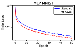
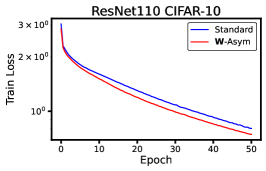
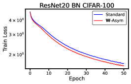
Figure 4: Bayesian neural network training loss over time for depth 8 MLPs on MNIST (left), ResNet110 on CIFAR-10 (middle), and ResNet20 with BatchNorm on CIFAR-100 (right). $\mathbf{W}$-Asymmetric networks train more quickly, and achieve lower training loss.

5.3 Metanetworks

Table 3: Metanetwork performance for predicting the test accuracy of small ResNets and our $\mathbf{W}$-Asym ResNets. Each row is a different metanetwork. Reported are $R^{2}$ and Kendall $\tau$ on the test set — higher is better.

	ResNet			$\mathbf{W}$-Asym ResNet
	$R^{2}$	$\tau$		$R^{2}$	$\tau$
MLP	$-.171\pm.11$	$.311\pm.02$		$\mathbf{.594}\pm.12$	$\mathbf{.864}\pm.01$
DMC [11]	$.950\pm.01$	$.787\pm.02$		$\mathbf{.967}\pm.01$	$\mathbf{.911}\pm.01$
DeepSets [73]	$.855\pm.01$	$.617\pm.03$		$\mathbf{.936}\pm.00$	$\mathbf{.858}\pm.00$
StatNN [63]	$.976\pm.00$	$.866\pm.00$		$\mathbf{.978}\pm.00$	$\mathbf{.935}\pm.01$

Background. Metanetworks [38] — also referred to as deep weight-space networks [44, 56], meta-models [34], or neural functionals [77, 78, 79] — are neural networks that take as inputs the parameters of other neural networks. Recent work has found that making metanetworks invariant or equivariant to parameter-space symmetries of the input neural networks can substantially improve metanetwork performance [44, 77, 38, 31].

Hypothesis. Asymmetric networks are easier to train metanetworks on because they do not have to explicitly account for symmetries.

Experimental setup. We experiment with metanetworks on the task of predicting the CIFAR-10 test accuracy of an input image classifier, which many metanetworks have been tested on [63, 11, 77, 38]. We use metanetworks based on simple MLPs, 1D-CNN metanetworks [11], and metanetworks that are exactly invariant to permutation parameter symmetries: DeepSets [73] and StatNN [63]. We train two separate datasets of 10,000 image classifiers: one dataset of small ResNet models, and one dataset of $\mathbf{W}$-Asymmetric ResNet models. More information on the data, metanetworks, and training details are in Appendix E.3.

Results. In Table 3, we see that metanetworks are signficantly better at predicting the performance of our $\mathbf{W}$-Asymmetric ResNets than standard ResNets. Interestingly, simple MLP metanetworks, which view the input parameters as a flattened vector, can predict the test accuracy of Asymmetric Networks quite well, but fail on standard networks. Also, the permutation equivariant metanetworks (DeepSets and StatNN) both improve on $\mathbf{W}$-Asym ResNets compared to on ResNets, even though the permutation symmetries of standard ResNets do not affect these metanetworks; thus, it may be possible that other symmetries in standard ResNets (but not Asym-ResNets) harm metanetwork performance, or they may be other factors besides symmetries that improve metanetwork performance for Asym-ResNets.

5.4 Monotonic Linear Interpolation

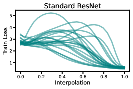
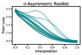
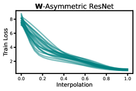
Figure 5: Train loss against interpolation coefficient $\alpha$ for the interpolation $(1-\alpha)\theta_{0}+\alpha\theta_{T}$ between initial parameters $\theta_{0}$ and trained parameters $\theta_{T}$. Trajectories for the 20 $(\theta_{0},\theta_{T})$ pairs of lowest train loss for each architecture are plotted. The trajectories for Asymmetric ResNets appear significantly more monotonic and convex.

Table 4: Monotonic linear interpolation: properties of linear interpolations between 300 pairs of initialization and trained parameters. Arrows denote behavior that is more similar to convex optimization, e.g. there is a downarrow $(\downarrow)$ next to $\Delta$ because convex objectives have nonpositive $\Delta$, while nonconvex can have positive $\Delta$. For both types of Asymmetric networks, all differences from Standard ResNets are statistically significant ($p<.001$) under a two-sided T-test: Asymmetric networks have significantly more monotonic and convex linear interpolations from initialization.

	$\Delta\downarrow$	Percent Monotonic $\uparrow$	Local Convexity $\uparrow$	Global Convexity $\uparrow$
Standard ResNet	$.079\pm.109$	$26.3\%$	$.548\pm.139$	$.823\pm.229$
$\sigma$-Asym ResNet	$.004\pm.047$	$87.3\%$	$.675\pm.143$	$.976\pm.098$
$\mathbf{W}$-Asym ResNet	$\mathbf{-.027}\pm.026$	$\mathbf{100\%}$	$\mathbf{.769}\pm.165$	$\mathbf{1.00}\pm.000$

Background. One common method of studying the loss landscapes of neural networks is by studying the one-dimensional line segment of parameters attained by linear interpolation between parameters at initialization and parameters after training. Many works have observed monotonic linear interpolation (MLI), which is when the training loss monotonically decreases along this line segment [20, 16, 40, 66]. Loss landscapes of convex problems have this property as well, so presence of the monotonic linear interpolation property has been used as a rough measure of how well-behaved the loss landscape is. However, with many types of models, tasks, or hyperparameter settings, monotonic linear interpolation does not hold [40, 66], or there is a large plateau where the loss barely changes for much of the line segment [16, 68]; neither of these properties can happen for convex objectives trained to completion. To the best of our knowledge, there has been little work on the role of parameter symmetries — or lack thereof — in monotonic linear interpolation (besides one minor experiment in [40] Appendix C.9). Nonetheless, since removing parameter symmetries substantially improves linear interpolation between trained networks (Section 5.1), one may expect removing parameter symmetries to improve monotonic linear interpolation.

Hypothesis. The training loss along the line segment between initialization and trained parameters is more monotonic and convex for Asymmetric networks.

Experimental setup. For the learning task, we follow the setup used for creating the dataset of image classifiers in Section 5.3. In particular, we train 300 standard ResNets and 300 $\mathbf{W}$-Asymmetric ResNets with varying hyperparameters sampled from the same distributions as used for the dataset of image classifiers (see Appendix Table 8). For each of these networks, we linearly interpolate between its initial parameters $\theta_{0}$ and its final trained parameters $\theta_{T}$: $(1-\alpha)\theta_{0}+\alpha\theta_{T}$ for 25 uniformly spaced values $0=\alpha_{1}<\alpha_{2}<\ldots<\alpha_{25}=1$. To measure monotonicity, we record the maximum increase between adjacent networks $\Delta=\max(L(\alpha_{i+1})-L(\alpha_{i}))$, and the percentage of networks that have $\Delta\leq 0$ i.e. the percentage of networks that satisfy monotonic linear interpolation. To measure convexity, we consider a local convexity measure (the proportion of $\alpha_{i}$ where the centered difference second derivative approximation is nonnegative) and a global convexity measure (the proportion of $\alpha_{i}$ such that $L(\alpha_{i})$ lies below the line segment between the endpoints, i.e. $L(\alpha_{i})\leq(1-\alpha_{i})L(0)+\alpha_{i}L(1)$).

Results. Table 4 shows the measures of monotonicity and convexity for standard, $\sigma$-Asymmetric, and $\mathbf{W}$-Asymmetric ResNets. Remarkably, every single one of the 300 $\mathbf{W}$-Asymmetric ResNets satisfies monotonic linear interpolation and has a trajectory that lies underneath the line segment between the endpoints. Qualitatively, we can see in Figure 5 that $\mathbf{W}$-Asymmetric ResNets do not have any clear loss barriers from initialization, nor any loss plateaus that indicate nonconvexity. In contrast, the majority of standard ResNets have non-monotonic trajectories, and the monotonic trajectories seem to be more nonconvex. $\sigma$-Asymmetric network trajectories are signficantly more convex and monotonic than standard network trajectories, but there are some non-monotonic or nonconvex trajectories still.

5.5 Other Optimization and Loss Landscape Properties

In Appendix A, we note other interesting differences in optimization and loss landscape properties of Asymmetric and standard neural networks. These can be summarized as:

1. Even though Asymmetric networks interpolate much better than standard networks, the parameters of trained Asymmetric networks are often basically the same distance away from each other in weight space as standard networks.

2. Asymmetric networks do not tend to overfit as much: the difference in train performance and test performance can be substantially lower than that of standard networks.

3. Asymmetric networks can take longer to train, especially when choosing hyperparameters that make them more dissimilar to standard networks.

6 Discussion

While many properties of Asymmetric networks are in line with our hypotheses and intuition about the impact of removing parameter symmetries, there are many unexpected effects and unanswered questions that are promising to further investigate. For instance, we did not extensively explore Asymmetric networks in the context of model interpretability, generalization measures in weight spaces, or optimization improvements, all of which are known to be influenced to some extent by parameter symmetries. Further studying the properties in Section 5.5, the dependence of behavior on the choices of Asymmetry-inducing hyperparameters, and other design choices in making networks asymmetric could also bring more insights into parameter space symmetries. We believe that future theoretical and empirical study of Asymmetric networks could garner many insights into the role of parameter symmetries in deep learning.

Acknowledgements

We would like to thank Kwangjun Ahn, Benjamin Banks, Nima Dehmamy, Nikos Karalias, Jinwoo Kim, Marc Law, Hannah Lawrence, Thien Le, Jonathan Lorraine, James Lucas, Behrooz Tahmasebi, and Logan Weber for discussions at various points of this project. DL is supported by an NSF Graduate Fellowship. RW is supported in part by NSF award 2134178. HM is the Robert J. Shillman Fellow, and is supported by the Israel Science Foundation through a personal grant (ISF 264/23) and an equipment grant (ISF 532/23). This research was supported in part by Office of Naval Research grant N00014-20-1-2023 (MURI ML-SCOPE), NSF AI Institute TILOS (NSF CCF-2112665), NSF award 2134108, and the Alexander von Humboldt Foundation.

Appendix A Additional Observations on Asymmetric Networks

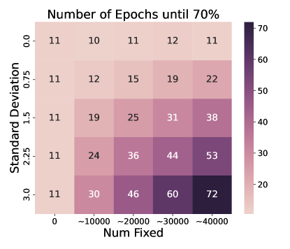
Figure 6: Epochs until reaching $70\%$ training accuracy on CIFAR-10 when varying the hyperparameters of $\mathbf{W}$-Asymmetric ResNets; we vary number of fixed entries $n_{\mathrm{fix}}$ and standard deviation $\kappa$ of the fixed entries $\mathbf{{\color[rgb]{.75,0,.25}F}}$. Entries further to the bottom and right are more asymmetric, while the entries further to the top and left are more like standard networks (the leftmost column are all standard networks). We see that more-asymmetric networks need more time to train.

There are several other interesting differences in the optimization and loss landscape properties of Asymmetric and standard neural networks. For one, even though Asymmetric networks generally interpolate significantly better than standard networks, this cannot be seen by measuring distances in parameter space. For instance, in GNN experiments following the setup of Section 5.1, pairs of standard GNNs have a distance per parameter of .000174 on average, whereas $\mathbf{W}$-Asymmetric GNNs have .000159, which is only slightly lower. However, the average test loss barrier is 1.448 for standard GNNs while it is only 0.069 for $\mathbf{W}$-Asymmetric GNNs. Likewise, in our datasets of 10,000 standard and $\mathbf{W}$-Asymmetric ResNets, the average distance per parameter between the weights of trained standard classifiers is .0034, which is actually lower than the distance per parameter of .0051 for $\mathbf{W}$-Asymmetric ResNets (estimated on 20,000 pairs of networks). Thus, although we sometimes imagine well-interpolating pairs of networks to lie in the same local basin of parameter space, $\mathbf{W}$-Asymmetric networks are actually rather far apart in parameter space, but nonetheless have linear segments of low loss between them.

We also find that Asymmetric networks often do not overfit as much as standard networks. For instance, in the GNN setup of Section 5.1, standard GNNs have a max training accuracy of $84.6\%$ on average, with a validation accuracy of $71.6\%$. On the other hand, $\sigma$-Asym GNNs have $70.8\%/70.1\%$ train/validation accuracy, while $\mathbf{W}$-Asym GNNs have $70.7\%/70.06\%$ train/validation accuracy. This difference does not show as much in our datasets of 10,000 standard ResNets and $\mathbf{W}$-Asym ResNets, possibly because of the substantial regularization (data augmentation, weight decay, and label smoothing) used for training (standard gets $74.8\%/73.8\%$ train/test accuracy while $\mathbf{W}$-Asymmetric gets $64.0\%/64.0\%$).

Further, in Figure 6, we see that training speed is slower for $\mathbf{W}$-Asymmetric ResNets when we increase the amount of asymmetry (by increasing the number of fixed entries and the standard deviation of the fixed entries). While standard ResNets take on average $11$ epochs to reach $70\%$ training accuracy on CIFAR-10, $\mathbf{W}$-Asymmetric ResNets with the most extreme hyperparameters take up to $72$ epochs.

Appendix B Proofs of Theoretical Results

B.1 Graph-based approach

Here, we prove that as long as each mask matrix $M$ in our $\mathbf{W}$-Asymmetric MLPs with fixed entries set to zero has unique nonzero rows, then our architecture has no nontrivial neural DAG automorphisms. In practice, we find that setting the standard deviation $\kappa$ of the fixed entries $\mathbf{{\color[rgb]{.75,0,.25}F}}$ to be positive (and in fact orders of magnitude larger than the standard deviation that we typically initialize trainable weights with) is important to achieve properties such as linear mode connectivity that Asymmetric networks have but standard networks do not have. When $\kappa=0$ (i.e. when fixed entries are set to zero), we can directly work in the framework of Lim et al. [38] that connects parameter symmetries to computation graph automorphisms. To work towards generalizing our result to $\kappa>0$, we would have to modify the definitions and results of Lim et al. [38]; for instance, we would need to add edges associated to untrainable parameters in the computation graph, and redefine the concept of neural DAG automorphisms. We leave such exploration to future work.

Theorem 3.

If each mask matrix $M$ has unique nonzero rows, then $\mathbf{W}$-Asymmetric MLPs with $\kappa=0$ have no nontrivial neural DAG automorphisms.

Proof.

Consider an $L$-layer $\mathbf{W}$-Asymmetric MLP with fixed entries set to zero. Denote its weights as $\mathbf{W}_{L},\ldots,\mathbf{W}_{1}$ and the corresponding binary masks as $M_{L},\ldots,M_{1}$. The forward pass of such a network on an input $x$ is then

$$[\mathbf{W}_{L}\odot M_{L}]\sigma(\cdots\sigma([\mathbf{W}_{1}\odot M_{1}]x)\cdots),$$ (5)

for some elementwise nonlinearity $\sigma$. The dimension of $\mathbf{W}_{i}$ is $d_{i}\times d_{i-1}$. In the framework of Lim et al. [38], this is a feedforward neural network with a computation graph defined as follows.

The node set is $V_{0}\times V_{1}\times\ldots\times V_{L}$, where $V_{i}$ has $d_{i}$ nodes, and no nodes are shared between different $V_{i}$. If a node $v$ is in $V_{i}$, then we say that $\mathrm{layer}(v)=i$. $V_{0}$ contains the input nodes and $V_{L}$ contains the output nodes. The adjacency matrix can be written as

$$A=\begin{bmatrix}0&\\ M_{1}&0\\ &M_{2}&\\ &&\ddots&0\\ &&&M_{L}&0\end{bmatrix}.$$ (6)

Every block besides the ones containing masks is zero. There are $L+1\times L+1$ blocks, and the $(i,j)$ block is of size $d_{i}\times d_{j}$.

Recall that a neural DAG automorphism is a relabelling of nodes $\tau\mathrel{\mathop{\mathchar 58\relax}}V\to V$ such that $\tau$ is bijective, $(i,j)\in E$ if and only if $(\tau(i),\tau(j))\in E$, and every input node and output node is a fixed point of $\tau$.

Now, let $\tau\mathrel{\mathop{\mathchar 58\relax}}V\to V$ be a neural DAG automorphism. Further, let $P$ be the corresponding permutation matrix. We will show that $\tau$ is the identity, i.e. that $P=I$. By Lemma 1, we know that $\tau$ preserves layer number of nodes, meaning $\mathrm{layer}(\tau(i))=\mathrm{layer}(i)$. Thus, $P$ is a block diagonal permutation matrix:

$$P=\begin{bmatrix}P_{0}\\ &P_{1}\\ &&\ddots\\ &&&P_{L}\\ \end{bmatrix},$$ (7)

where $P_{i}$ is $d_{i}\times d_{i}$. Morever, $P_{0}=I$ and $P_{L}=I$ because input nodes and output nodes are fixed points. Applying this to the adjacency matrix, we see that

$$\tau(A)=PAP^{\top}=\begin{bmatrix}0&\\ P_{1}M_{1}P_{0}^{\top}&0\\ &&&\ddots\\ &&&P_{L}M_{L}P_{L-1}^{\top}&0\end{bmatrix}.$$ (8)

Since $\tau$ is a neural DAG automorphism, we have that $\tau(A)=A$. Equating blocks, this means that $P_{1}M_{1}P_{0}^{\top}=M_{1}$. As $P_{0}=I$, we have $P_{1}M_{1}=M_{1}$. But $M_{1}$ has unique rows, so $P_{1}=I$ as well.

For the inductive step, assume $P_{i}=I$ for some $i$. Then $P_{i+1}M_{i+1}P_{i}^{\top}=P_{i+1}M_{i+1}=M_{i+1}$, so since $M_{i+1}$ has unique rows, we have that $P_{i+1}=I$. As this holds for any $i$ by induction, this means that $P=I$, so $\tau$ is a trivial neural DAG automorphism and we are done. ∎

Lemma 1.

Neural DAG automorphisms preserve layer number in $\mathbf{W}$-Asymmetric MLPs that have masks with nonzero rows.

Proof.

Let $\tau$ be a neural DAG automorphism. This means that $PAP^{\top}=A$, where $P$ is the permutation matrix associated to $\tau$. Then, using $PAP^{\top}=A$ for the first equality and the definition of $P$ in the second, we have that

$$A_{\tau(i),\tau(j)}=(PAP^{\top})_{\tau(i),\tau(j)}=A_{i,j}.$$ (9)

We proceed by induction on layer number $l$. For any input node $i$ we know that $\tau(i)=i$, so of course $\mathrm{layer}(\tau(i))=\mathrm{layer}(i)$.

Now, suppose that $\mathrm{layer}(\tau(i))=\mathrm{layer}(i)$ for any $i$ in layer $l\geq 1$. If node $j$ is in layer $l+1$, then there is some $i$ in layer $l$ such that $(i,j)\in E$ because $M_{l+1}$ has no nonzero rows. We have that $A_{\tau(i),\tau(j)}=A_{i,j}$, so $\tau(i)$ is connected to $\tau(j)$. As we know that $\tau(i)$ is in layer $l$, we have that $\tau(j)$ is in layer $l+1$. ∎

B.2 Symmetry Breaking via Nonlinearities

Proposition 3.

Let the parameter space $\Theta$ be all pairs of square invertible matrices $\theta=(\mathbf{W}_{2},\mathbf{W}_{1})$ for $\mathbf{W}_{2},\mathbf{W}_{1}\in GL(d)$, and let $f_{\theta}(x)=\mathbf{W}_{2}\sigma(\mathbf{W}_{1}x)$. If $\sigma$ has no linear equivariances, then $f_{\theta_{1}}=f_{\theta_{2}}$ if and only if $\theta_{1}=\theta_{2}$. In other words, there are no nontrivial parameter space symmetries.

Proof.

If $\theta_{1}=\theta_{2}$, then clearly $f_{\theta_{1}}=f_{\theta_{2}}$. For the other direction, suppose $f_{\theta_{1}}=f_{\theta_{2}}$, and denote $\theta_{1}=(\mathbf{W}_{2},\mathbf{W}_{1})$ and $\theta_{2}=(\widetilde{\mathbf{W}}_{2},\widetilde{\mathbf{W}}_{1})$. Then for any input $z\in\mathbb{R}^{n}$, we have

$$\mathbf{W}_{2}\sigma(\mathbf{W}_{1}z) =\widetilde{\mathbf{W}}_{2}\sigma(\widetilde{\mathbf{W}}_{1}z)$$ (10)

$$\widetilde{\mathbf{W}}_{2}^{-1}\mathbf{W}_{2}\sigma(\mathbf{W}_{1}z) =\sigma(\widetilde{\mathbf{W}}_{1}z).$$ (11)

Now, choose an arbitrary $x\in\mathbb{R}^{n}$. We let $z$ in the above equation (11) be $\mathbf{W}_{1}^{-1}x$, so we have

$$\widetilde{\mathbf{W}}_{2}^{-1}\mathbf{W}_{2}\sigma(x) =\sigma(\widetilde{\mathbf{W}}_{1}\mathbf{W}_{1}^{-1}x).$$ (12)

This holds for any $x$, so $\widetilde{\mathbf{W}}_{2}^{-1}\mathbf{W}_{2}\circ\sigma=\sigma\circ\widetilde{\mathbf{W}}_{1}\mathbf{W}_{1}^{-1}$, i.e. we have found a linear equivariance of $\sigma$. Since $\sigma$ has no linear equivariances,

$$\widetilde{\mathbf{W}}_{2}^{-1}\mathbf{W}_{2}=I=\widetilde{\mathbf{W}}_{1}\mathbf{W}_{1}^{-1},$$ (13)

meaning that $\widetilde{\mathbf{W}}_{2}=\mathbf{W}_{2}$ and $\widetilde{\mathbf{W}}_{1}=\mathbf{W}_{1}$, i.e. $\theta_{1}=\theta_{2}$, so we are done. ∎

B.2.1 FiGLU nonlinearity proofs (Proposition 2)

Now, we study the properties of our FiGLU nonlinearity $\sigma(x)=\eta(\mathbf{{\color[rgb]{.75,0,.25}F}}x)\odot x$, where $\eta$ is the sigmoid function $\eta(x)=\frac{1}{1+e^{-x}}$. For proving Proposition 2, we want to prove that with probability 1 over samples of $\mathbf{{\color[rgb]{.75,0,.25}F}}$, $\sigma$ has no permutation or diagonal equivariances.

We say that $\sigma$ has no permutation equivariances if whenever $P_{2}\circ\sigma=\sigma\circ P_{1}$ for permutation matrices $P_{1}$ and $P_{2}$, then $P_{1}=P_{2}=I$. Likewise, we say that $\sigma$ has no diagonal equivariances if whenever $B\circ\sigma=\sigma\circ A$ for invertible diagonal matrices $A$ and $B$, then $A=B=I$.

We will show that these two properties hold for any $\mathbf{{\color[rgb]{.75,0,.25}F}}$ that has no permutation symmetries and no zero entries. We say that $\mathbf{{\color[rgb]{.75,0,.25}F}}$ has no permutation symmetries if $P_{2}\mathbf{{\color[rgb]{.75,0,.25}F}}P_{1}=\mathbf{{\color[rgb]{.75,0,.25}F}}$ for permutation matrices $P_{1}$ and $P_{2}$ implies that $P_{1}=P_{2}=I$. Note that if $\mathbf{{\color[rgb]{.75,0,.25}F}}$ has distinct entries, then it has no permutation symmetries. Thus, $\mathbf{{\color[rgb]{.75,0,.25}F}}$ satisfies both of these conditions with probability 1, since the set of matrices with nondistinct entries or with at least one zero entry are of Lebesgue measure zero, so they have zero probability under the Gaussian distribution. We now proceed to show that $\sigma$ has no permutation or diagonal equivariances under these conditions on $\mathbf{{\color[rgb]{.75,0,.25}F}}$.

Proposition 4.

If $\mathbf{{\color[rgb]{.75,0,.25}F}}$ is a square matrix with no permutation symmetries, then $\sigma(x)=\eta(\mathbf{{\color[rgb]{.75,0,.25}F}}x)\odot x$ has no permutation equivariances.

Proof.

Suppose $\sigma\circ P_{1}=P_{2}\circ\sigma$ for permutation matrices $P_{1},P_{2}$. We will show that $P_{1}=P_{2}=I$. For any input $x$, we have

$$\eta(\mathbf{{\color[rgb]{.75,0,.25}F}}P_{1}x)\odot P_{1}x =P_{2}\left[\eta(\mathbf{{\color[rgb]{.75,0,.25}F}}x)\odot x\right]$$ (14)

$$P_{2}^{\top}\left[\eta(\mathbf{{\color[rgb]{.75,0,.25}F}}P_{1}x)\odot P_{1}x\right] =\eta(\mathbf{{\color[rgb]{.75,0,.25}F}}x)\odot x$$ (15)

$$\eta(P_{2}^{\top}\mathbf{{\color[rgb]{.75,0,.25}F}}P_{1}x)\odot P_{2}^{\top}P_{1}x =\eta(\mathbf{{\color[rgb]{.75,0,.25}F}}x)\odot x,$$ (16)

where we used permutation equivariance of $\eta$, which acts elementwise. Let $x=e_{i}$, the standard basis vector that is $1$ in the $i$th coordinate and $0$ elsewhere. If $i$ is not a fixed point of the permutation $P_{2}^{\top}P_{1}$, then let $j$ be the index that it is mapped to. Then equation (16) gives that

$$\eta(P_{2}^{\top}\mathbf{{\color[rgb]{.75,0,.25}F}}P_{1}e_{i})\odot P_{2}^{\top}P_{1}e_{i} =\eta(\mathbf{{\color[rgb]{.75,0,.25}F}}e_{i})\odot e_{i}$$ (17)

$$\eta(P_{2}^{\top}\mathbf{{\color[rgb]{.75,0,.25}F}}P_{1}e_{i})\odot e_{j} =\eta(\mathbf{{\color[rgb]{.75,0,.25}F}}e_{i})\odot e_{i}.$$ (18)

In the $i$th coordinate of this equality of vectors, we see that $\eta(\mathbf{{\color[rgb]{.75,0,.25}F}}e_{i})=0$, which is impossible, since $\eta$ is the sigmoid function. Thus, $i$ cannot be a fixed point of $P_{2}^{\top}P_{1}$, so $P_{2}^{\top}P_{1}=I$ is the identity permutation. Now, let $x$ be an arbitrary vector with no zero entries. Equation (16) gives that

$$\eta(P_{2}^{\top}\mathbf{{\color[rgb]{.75,0,.25}F}}P_{1}x)\odot x =\eta(\mathbf{{\color[rgb]{.75,0,.25}F}}x)\odot x.$$ (19)

Since $x$ is nonzero, we can divide by $x_{i}$ in the $i$th coordinate of this vector equality for each $i$ to get that

$$\eta(P_{2}^{\top}\mathbf{{\color[rgb]{.75,0,.25}F}}P_{1}x)=\eta(\mathbf{{\color[rgb]{.75,0,.25}F}}x).$$ (20)

As $\eta$ is bijective,

$$P_{2}^{\top}\mathbf{{\color[rgb]{.75,0,.25}F}}P_{1}x=\mathbf{{\color[rgb]{.75,0,.25}F}}x.$$ (21)

Because this holds for all $x$ with no zero entries (and in particular for a basis of the input space), we know that

$$P_{2}^{\top}\mathbf{{\color[rgb]{.75,0,.25}F}}P_{1}=\mathbf{{\color[rgb]{.75,0,.25}F}}$$ (22)

as matrices. But since $\mathbf{{\color[rgb]{.75,0,.25}F}}$ has no permutation symmetries, we have that $P_{1}=P_{2}=I$, so we are done. ∎

Proposition 5.

If $\mathbf{{\color[rgb]{.75,0,.25}F}}$ is a square matrix with no zero entries, then $\sigma(x)=\eta(\mathbf{{\color[rgb]{.75,0,.25}F}}x)\odot x$ has no diagonal equivariances.

Proof.

Let $A=\mathrm{Diag}(\alpha)$ and $B=\mathrm{Diag}(\beta)$ be invertible diagonal matrices, and suppose that $\sigma\circ A=B\circ\sigma$. We will show that $A=B=I$. For any input $x$, we have

$$\eta(\mathbf{{\color[rgb]{.75,0,.25}F}}[\alpha\odot x])\odot(\alpha\odot x) =\beta\odot\left[\eta(\mathbf{{\color[rgb]{.75,0,.25}F}}x)\odot x\right].$$ (23)

Let $x=ce_{i}$, where $e_{i}$ is the $i$th standard basis vector and $c\neq 0$ is any nonzero number. Then

$$\eta(\mathbf{{\color[rgb]{.75,0,.25}F}}c\alpha_{i}e_{i})\odot c\alpha_{i}e_{i} =\beta\odot\left[\eta(c\mathbf{{\color[rgb]{.75,0,.25}F}}e_{i})\odot ce_{i}\right].$$ (24)

At the $i$th coordinate of this equality, we have

$$\eta(\mathbf{{\color[rgb]{.75,0,.25}F}}c\alpha_{i}e_{i})_{i}c\alpha_{i} =\beta_{i}\eta(c\mathbf{{\color[rgb]{.75,0,.25}F}}e_{i})_{i}c$$ (25)

$$\frac{\alpha_{i}}{\beta_{i}} =\frac{\eta(c\mathbf{{\color[rgb]{.75,0,.25}F}}e_{i})_{i}}{\eta(\alpha_{i}c\mathbf{{\color[rgb]{.75,0,.25}F}}e_{i})_{i}}$$ (26)

Thus, the right hand side is constant in $c$. We must have that $\alpha_{i}>0$, because if not, then increasing $c$ would increase either the numerator or denominator and decrease the other, hence contradicting the equality (here we use that $\mathbf{{\color[rgb]{.75,0,.25}F}}$ has no zero entries, so $c\mathbf{{\color[rgb]{.75,0,.25}F}}e_{i}$ is nonzero in every entry). Thus, letting $c\to\infty$, we see that $\frac{\alpha_{i}}{\beta_{i}}=1$, so $\alpha_{i}=\beta_{i}$. Plugging this back into Equation (26), we have

$$1 =\frac{\eta(c\mathbf{{\color[rgb]{.75,0,.25}F}}e_{i})_{i}}{\eta(\alpha_{i}c\mathbf{{\color[rgb]{.75,0,.25}F}}e_{i})_{i}}$$ (27)

$$\eta(\alpha_{i}c\mathbf{{\color[rgb]{.75,0,.25}F}}e_{i})_{i} =\eta(c\mathbf{{\color[rgb]{.75,0,.25}F}}e_{i})_{i}$$ (28)

$$\alpha_{i}c(\mathbf{{\color[rgb]{.75,0,.25}F}}e_{i})_{i} =c(\mathbf{{\color[rgb]{.75,0,.25}F}}e_{i})_{i}$$ (29)

$$\alpha_{i} =1,$$ (30)

where in the third line we used the fact that $\eta$ is invertible. We have shown that $\alpha_{i}=\beta_{i}=1$ for each $i$, so $A=B=I$ and we are done. ∎

We note that the proofs of these two results about FiGLU are reminiscent of some proof techniques from Godfrey et al. [19], such as those used in their analysis of $\mathrm{GELU}$ nonlinearities.

B.3 Proofs for Universal Approximation

Here, we prove the universal approximation result for our $\mathbf{W}$-Asymmetric MLPs.

Theorem 4.

Let $\eta$ be any nonpolynomial elementwise nonlinearity with $\eta(x)-\eta(-x)=x$ (e.g. $\mathrm{ReLU},\mathrm{GELU},\mathrm{swish}$), let $\Omega\subseteq\mathbb{R}^{D}$ be a compact domain, and let $f_{\mathrm{target}}\mathrel{\mathop{\mathchar 58\relax}}\Omega\to\mathbb{R}$ be a continuous target function. Fix $\varepsilon>0$ and $\delta>0$.

There exists a width $n^{\prime}$ such that for all $n>n^{\prime}$, with probability $1-\delta$, for a randomly sampled 4-layer $\mathbf{W}$-Asymmetric MLP $f$ with $\eta$ nonlinearity, hidden dimensions $24n\rightarrow n\rightarrow 24n$, and $n_{\mathrm{fix}}\in o(n^{1/4})$ hardwired entries per neuron, there will exist $\theta\in\Theta$ such that the $\mathbf{W}$-Asymmetric MLP $f\mathrel{\mathop{\mathchar 58\relax}}\mathbb{R}^{n}\to\mathbb{R}$ approximates $f_{\mathrm{target}}$ to $\varepsilon$:

$$\mathinner{\!\left\lVert f_{\theta}([x;0])-f_{\mathrm{target}}(x)\right\rVert}<\varepsilon\text{ for all }x\in\Omega.$$ (31)

Importantly, we require that the input to $f_{\theta}$ be padded with $n-D$ zeroes, so $[x;0]\in\mathbb{R}^{n}$.

B.3.1 Proof sketch

To approximate $f_{\mathrm{target}}$ to $\varepsilon>0$, we will leverage the universal approximation for standard MLPs with nonlinearity $\eta$ to first obtain a standard 2-layer MLP that approximates $f_{\mathrm{target}}$ to within $\varepsilon$, meaning $\mathinner{\!\left\lVert f_{\mathrm{target}}(x)-f_{\mathrm{MLP}}(x)\right\rVert}<\varepsilon$ for all $x\in\Omega$. Then we will exactly represent $f_{\mathrm{MLP}}$ using an Asymmetric Network $f$.

This will be done by approximating each linear map $W$ of $f_{\mathrm{MLP}}$ by two layers of an Asymmetric network: $W^{\prime}_{2}\circ\eta\circ W^{\prime}_{1}=W$ for Asymmetric linear maps $W^{\prime}_{2}$ and $W^{\prime}_{1}$. For the sake of exposition, we will show how to do this first when both $W^{\prime}_{2}$ and $W^{\prime}_{1}$ have no Asymmetric mask (i.e. fitting a linear map $W$ using a standard two-layer $\eta$-MLP), then when only $W^{\prime}_{2}$ has an Asymmetric mask, and finally when both $W^{\prime}_{2}$ and $W^{\prime}_{1}$ have an Asymmetric mask.

B.3.2 Fitting a Linear Map with a Two-Layer Standard MLP

Let $W\in\mathbb{R}^{n\times n}$ be the target linear map, and let $B\in\mathbb{R}^{2n\times n}$ and $A\in\mathbb{R}^{n\times 2n}$ be parameters of a two-layer MLP, defined by $f_{A,B}(x)=A\eta(Bx)$. We will choose $A$ and $B$ such that $f_{A,B}(x)=Wx$ for all $x\in\mathbb{R}^{n}$.

Denote the $i$th row of $W$ by $W_{i}$, so that

$$W=\begin{bmatrix}W_{0}\\ \vdots\\ W_{n-1}\end{bmatrix},\qquad Wx=\begin{bmatrix}W_{0}\cdot x\\ \vdots\\ W_{n-1}\cdot x\\ \end{bmatrix}$$ (32)

We set $A$ and $B$ as follows, where $I_{n}$ is the $n\times n$ identity matrix:

$$A=I_{n}\otimes\begin{bmatrix}1&-1\end{bmatrix}=\begin{bmatrix}1&-1\\ &&1&-1\\ &&&\ddots&\ddots\\ &&&&1&-1\end{bmatrix}\qquad B=\begin{bmatrix}W_{0}\\ -W_{0}\\ W_{1}\\ -W_{1}\\ \vdots\\ W_{n-1}\\ -W_{n-1}\end{bmatrix}.$$ (33)

Then we can see that $f_{A,B}$ exactly computes the linear transformation $Wx$.

$$A\eta(Bx)=\begin{bmatrix}\eta(W_{0}\cdot x)-\eta(-W_{0}\cdot x)\\ \vdots\\ \eta(W_{n-1}\cdot x)-\eta(-W_{n-1}\cdot x)\\ \end{bmatrix}=\begin{bmatrix}W_{0}\cdot x\\ \vdots\\ W_{n-1}\cdot x\\ \end{bmatrix}=Wx.$$ (34)

B.3.3 Fitting a Linear Map with One Asymmetric and One Standard Linear Map

Let $n_{\mathrm{fix}}>0$ and let each row of $\mathbf{{\color[rgb]{.75,0,.25}N}}\in\{0,1\}^{n\times 6n}$ have $n_{\mathrm{fix}}$ entries equal to 0, selected at random. Let $B\in\mathbb{R}^{6n\times n}$ and $A\in\mathbb{R}^{n\times 6n}$. Define $A^{\prime}$ to be an Asymmetric linear map: $A^{\prime}=A\odot\mathbf{{\color[rgb]{.75,0,.25}N}}+(1-\mathbf{{\color[rgb]{.75,0,.25}N}})\odot\mathbf{{\color[rgb]{.75,0,.25}P}}$, where $\mathbf{{\color[rgb]{.75,0,.25}N}}$ is a randomly sampled binary mask, and $\mathbf{{\color[rgb]{.75,0,.25}P}}$ a randomly sampled Gaussian matrix. We consider a two-layer network with one Asymmetric and one standard linear map: $f_{A,B}(x)=A^{\prime}\eta(Bx)$. We want $f_{A,B}(x)=Wx$ for all x. For the remainder of this proof, we will assume that $\mathbf{{\color[rgb]{.75,0,.25}N}}$ never has three consecutive entries in a row set to zero; we will later show that this holds with high probability over the sampling of $\mathbf{{\color[rgb]{.75,0,.25}N}}$.

First, we define $B$ in a similar way to the purely linear setting, but with additional copies of entries to allow for error correction of the random noisy entries fixed in $A^{\prime}$.

$$B=\begin{bmatrix}W_{0}\\ W_{0}\\ W_{0}\\ -W_{0}\\ -W_{0}\\ -W_{0}\\ \vdots\\ W_{n-1}\\ W_{n-1}\\ W_{n-1}\\ -W_{n-1}\\ -W_{n-1}\\ -W_{n-1}\\ \end{bmatrix}.$$ (35)

Recall that each row $A_{i}^{\prime}$ of $A^{\prime}$ has $n_{\mathrm{fix}}$ entries that are randomly hardwired to constants. Ideally, we would want $A_{i}^{\prime}$ to pick out $\eta(W_{i}\cdot x)-\eta(-W_{i}\cdot x)=W_{i}\cdot x$, but because of the hardwired constants, $A_{i}^{\prime}$ might randomly add $c*\eta(W_{j}\cdot x)$. However, since there are three copies of $\eta(W_{j}\cdot x)$ in $\eta(Bx)$, as long as not all three corresponding entries in $A_{i}^{\prime}$ are fixed, one of the un-fixed copies can be changed such that the coefficients sum to $0$. Since by our assumption $\mathbf{{\color[rgb]{.75,0,.25}N}}$ never has three consecutive entries all set to 0, the coefficients of $A$ can be picked such that $A^{\prime}\eta(Bx)=Wx$. For example, a possible $A^{\prime}$ matrix would be

$$A^{\prime}=\setcounter{MaxMatrixCols}{21}\begin{bmatrix}1&0&0&-1&0&0&|&\mathbf{{\color[rgb]{.75,0,.25}1.1}}&\mathbf{{\color[rgb]{.75,0,.25}.37}}&-1.47&0&0&0&|\dots&|&0&0&0&0&0&0\\ .89&\mathbf{{\color[rgb]{.75,0,.25}-.89}}&0&0&0&0&|&\mathbf{{\color[rgb]{.75,0,.25}.37}}&.63&0&-1&0&0&|\dots&|&0&0&0&0&0&0\\ 0&0&0&0&0&0&|&0&0&0&0&0&0&|\dots&|&1&0&0&-1&0&0\\ \end{bmatrix}$$

Thus we have shown that under the assumption that $\mathbf{{\color[rgb]{.75,0,.25}N}}$ never has three consecutive entries equal to 0, $A$ can be picked such that $A^{\prime}\eta(Bx)=Wx$. We will now show that $\mathbb{P}(\mathbf{{\color[rgb]{.75,0,.25}N}}\text{ never has three consecutive entries equal to 0})$ can be made arbitrarily small by increasing the width $n$ while keeping $n_{\mathrm{fix}}$ to be $o(n^{1/3})$.

The probability there are three consecutive entries in a given row of $\mathbf{{\color[rgb]{.75,0,.25}N}}$ that are zero is $O(\frac{n_{\mathrm{fix}}^{3}}{n^{2}})$. By the union bound, the probability that any row has 3 consecutive hardwired entries is $O(\frac{n_{\mathrm{fix}}^{3}}{n})$. For any $n_{\mathrm{fix}}\in o(n^{1/3})$, this tends towards $0$. Thus, with probability $\geq 1-O(\frac{n_{\mathrm{fix}}^{3}}{n})$, $A$ can be picked such that $A^{\prime}\eta(Bx)=Wx$.

B.3.4 Fitting a Linear Map with Two Asymmetric Linear Maps

Once again let $n_{\mathrm{fix}}>0$, and let each row of $\mathbf{{\color[rgb]{.75,0,.25}M}}$ have $n_{\mathrm{fix}}$ entries equal to 0, selected at random. Let $B\in\mathbb{R}^{24n\times n}$ and $A\in\mathbb{R}^{n\times 24n}$. Further, define Asymmetric maps

$$A^{\prime}=A\odot\mathbf{{\color[rgb]{.75,0,.25}N}}+(1-\mathbf{{\color[rgb]{.75,0,.25}N}})\odot\mathbf{{\color[rgb]{.75,0,.25}P}},\qquad B^{\prime}=B\odot\mathbf{{\color[rgb]{.75,0,.25}M}}+(1-\mathbf{{\color[rgb]{.75,0,.25}M}})\odot\mathbf{{\color[rgb]{.75,0,.25}Q}},$$ (36)

where $\mathbf{{\color[rgb]{.75,0,.25}N}},\mathbf{{\color[rgb]{.75,0,.25}M}}$ are randomly sampled masks, and $\mathbf{{\color[rgb]{.75,0,.25}P}},\mathbf{{\color[rgb]{.75,0,.25}Q}}$ are normal matrices. Then we let $f_{A,B}(x)=A^{\prime}\eta(B^{\prime}(x))$, and we once again desire choices of parameters $A$ and $B$ such that $f_{A,B}(x)=Wx$.

Constructing $B$

Consider the randomly drawn mask $\mathbf{{\color[rgb]{.75,0,.25}M}}\in\{0,1\}^{24n\times n}$, and denote the $i$th row by $M_{i}$.

$$\mathbf{{\color[rgb]{.75,0,.25}M}}=\begin{bmatrix}M_{0}\\ M_{1}\\ \vdots\\ M_{24n-1}\end{bmatrix}$$ (37)

where $M_{i}\in\{0,1\}^{n}$. We partition $\mathbf{{\color[rgb]{.75,0,.25}M}}$’s rows into $n$ blocks of $24$ rows. $\beta_{1}=\{M_{0}\dots M_{23}\},\ldots\beta_{i}=\{M_{24i}\dots M_{24i+23}\}$. Now, consider $\beta_{1}$, the first $24$ rows of $\mathbf{{\color[rgb]{.75,0,.25}M}}$.

Definition B.1.

We say two rows $M_{j},\ M_{k}$ are intersecting if there is some column index $\alpha$ such that $M_{j,\alpha}=M_{k,\alpha}=0$. That is, two rows of are intersecting if they share a 0 at the same index.

Note that for any two given rows of $M$, the probability that they share a $0$ in the same location is $\leq\frac{n_{\mathrm{fix}}^{2}}{n}$.

We assume that $\beta_{i}$ contains no more than one pair of intersecting rows; later, we show this to hold with high probability. Then, every $\beta_{i}$ can be broken into two disjoint sets of 12 rows, $\beta_{i,0}$ and $\beta_{i,1}$, such that neither set of 12 contains a single pair of intersecting rows. Intuitively, this means that each row in $B$ corresponding to $\beta_{i,0}$ will have unique fixed indices.

Our goal will be for the rows in $\beta_{i}$ to mimic the row $W_{i}$. We will show how to do this for each $i$. Fix an arbitrary index $i\in\{0,\ldots,n-1\}$.

Without loss of generality, assume $\beta_{i,0}$ and $\beta_{i,1}$ are continguous, so $\beta_{i,0}=M_{24i\mathrel{\mathop{\mathchar 58\relax}}24i+11}$ and $\beta_{i,1}=M_{24i+11\mathrel{\mathop{\mathchar 58\relax}}24i+23}$. By our assumption, for $j,k\in\beta_{i,0}$ (i.e. $j,k\in\{0,\ldots,11\}$), the mask rows $M_{24i+j}$ and $M_{24i+k}$ are never $0$ in the same two column indices. Similarly, for $j,k\in\beta_{i,1}$ (i.e. $j,k\in\{12,\ldots,23\}$), the mask rows $M_{24i+j}$ and $M_{24i+k}$ are never $0$ in the same two column indices.

Next, we define $c_{i,j}$ as the difference between $B^{\prime}$ and $B$ in the $(24i+j)$th row:

$$c_{i,j}=B^{\prime}_{24i+j}-B_{24i+j}.$$ (38)

In particular, we have that

$$c_{i,j}=-B_{24i+j}\odot(1-M_{24i+j})+(1-M_{24i+j})\odot Q_{24i+j}.$$ (39)

Lemma 2.

For any indices $j\neq k$ such that $j,k\in\beta_{i,0}$ or $j,k\in\beta_{i,1}$, we have that

$$c_{i,j}\odot M_{24i+k}=c_{i,j}.$$ (40)

Proof.

By the definition of $c_{i,j}$, we know that $c_{i,j}$ is only nonzero at indices where $M_{24i+j}$ is equal to zero. Since $j,k$ are either both in $\beta_{i,0}$ or $\beta_{i,1}$, we know that $M_{24i+k}$ cannot also be zero at indices where $M_{24i+j}$ is zero. Thus, $M_{24i+k}$ is equal to $1$ at every index where $c_{i,j}$ is nonzero, so $c_{i,j}\odot M_{24i+k}=c_{i,j}$ as desired. ∎

Next, we construct $B$, by constructing this block of 24 rows. Let $[\mathbf{c}_{i,0},\mathbf{c}_{i,1},\mathbf{c}_{i,2},\mathbf{c}_{i,3}]$ be continguous sums of length-3 segments of $c_{i,\mathrel{\mathop{\mathchar 58\relax}}}$:

$$\mathbf{c}_{i,0} =c_{i,0}+c_{i,1}+c_{i,2}$$ (41)

$$\mathbf{c}_{i,1} =c_{i,3}+c_{i,4}+c_{i,5}$$ (42)

$$\mathbf{c}_{i,2} =c_{i,6}+c_{i,7}+c_{i,8}$$ (43)

$$\mathbf{c}_{i,3} =c_{i,9}+c_{i,10}+c_{i,11}$$ (44)

We assign the first 12 rows of $B$ as follows.

$$(0\leq j<3) \rightarrow B_{24i+j}=W_{i}+\mathbf{c}_{i,0}-\mathbf{c}_{i,1}+\mathbf{c}_{i,2}-\mathbf{c}_{i,3}-c_{ij}$$ (45)

$$(3\leq j<6) \rightarrow B_{24i+j}=-W_{i}-\mathbf{c}_{i,0}+\mathbf{c}_{i,1}-\mathbf{c}_{i,2}+\mathbf{c}_{i,3}-c_{ij}$$ (46)

$$(6\leq j<9) \rightarrow B_{24i+j}=+\mathbf{c}_{i,0}-\mathbf{c}_{i,1}+\mathbf{c}_{i,2}-\mathbf{c}_{i,3}-c_{ij}$$ (47)

$$(9\leq j<12) \rightarrow B_{24i+j}=-\mathbf{c}_{i,0}+\mathbf{c}_{i,1}-\mathbf{c}_{i,2}+\mathbf{c}_{i,3}-c_{ij}$$ (48)

Defining $\mathbf{c}=\mathbf{c}_{i,0}-\mathbf{c}_{i,1}+\mathbf{c}_{i,2}-\mathbf{c}_{i,3}$, we have the nice property:

$$(0\leq j<3) \rightarrow B^{\prime}_{24i+j}=W_{i}+\mathbf{c}$$ (49)

$$(3\leq j<6) \rightarrow B^{\prime}_{24i+j}=-W_{i}-\mathbf{c}$$ (50)

$$(6\leq j<9) \rightarrow B^{\prime}_{24i+j}=+\mathbf{c}$$ (51)

$$(9\leq j<12) \rightarrow B^{\prime}_{24i+j}=-\mathbf{c}$$ (52)

By the construction above, $B_{24i}^{\prime}=-B_{24i+3}^{\prime}$, and $B_{24i+6}^{\prime}=-B_{24i+9}^{\prime}$. This means that

$$\eta(B_{24i}^{\prime}\cdot x)-\eta(B_{24i+3}^{\prime}\cdot x)=B_{24i}^{\prime}\cdot x=(W_{i}+\mathbf{c})\cdot x$$ (53)

and likewise that

$$\eta(B_{24i+6}^{\prime}\cdot x)-\eta(B_{24i+9}^{\prime}\cdot x)=\mathbf{c}\cdot x$$ (54)

So that a simple linear map gives our desired output:

$$\eta(B_{24i}^{\prime}\cdot x)-\eta(B_{24i+3}^{\prime}\cdot x)-[\eta(B_{24i+6}^{\prime}\cdot x)-\eta(B_{24i+9}^{\prime}\cdot x)] =(W_{i}+\mathbf{c}-\mathbf{c})\cdot x$$ (55)

$$=W_{i}\cdot x.$$ (56)

In the next part, we will construct $A^{\prime}$ to compute this linear map, which will follow the method of Appendix B.3.3 (because $A^{\prime}$ has certain fixed entries).

What remains is to define the rows of $B$ corresponding to $\beta_{i,1}$ in an error correctible manner. This can be done easily by defining

$$\mathbf{d}=\sum_{j=12}^{23}c_{ij}$$ (57)

and then defining

$$(12\leq j<24)\rightarrow B_{24i+j}=\mathbf{d}-c_{ij}$$ (58)

By similar reasoning to before, this means that

$$(12\leq j<24)\rightarrow B^{\prime}_{24i+j}=\mathbf{d}.$$ (59)

Recall that we constructed $B^{\prime}$ under the assumption that no $\beta_{i}$ has at most one pair of intersecting rows. We now show that the $\beta_{i}$ each have at most one pair of intersecting rows with high probability. Within the $24$ rows of any given $\beta_{i}$, the probability that more than one pair of rows are intersecting is $\leq C\frac{n_{\mathrm{fix}}^{4}}{n^{2}}$ for some constant $C$. So, by the union bound, the probability over $M$ that any of the $\beta_{i}$ have more than one pair of intersecting rows is $\leq C\frac{n_{\mathrm{fix}}^{4}}{n}$. Thus, we can construct $B$ in this manner with probability $\geq 1-C\frac{n_{\mathrm{fix}}^{4}}{n}$. For sufficiently large $n$ and $n_{\mathrm{fix}}\in o(n^{1/4})$, this probability approaches $1$.

Construction of $A$

With our above construction, each block of the 24 rows in $\beta_{i}$ of $\eta(B^{\prime}x)$ is of the form

$$\begin{bmatrix}\eta((W_{i}+\mathbf{c})\cdot x)\\ \eta((W_{i}+\mathbf{c})\cdot x)\\ \eta((W_{i}+\mathbf{c})\cdot x)\\ \eta((-W_{i}-\mathbf{c})\cdot x)\\ \eta((-W_{i}-\mathbf{c})\cdot x)\\ \eta((-W_{i}-\mathbf{c})\cdot x)\\ \eta(\mathbf{c}\cdot x)\\ \eta(\mathbf{c}\cdot x)\\ \eta(\mathbf{c}\cdot x)\\ \eta(-\mathbf{c}\cdot x)\\ \eta(-\mathbf{c}\cdot x)\\ \eta(-\mathbf{c}\cdot x)\\ \eta(\mathbf{d}\cdot x)\\ \eta(\mathbf{d}\cdot x)\\ \eta(\mathbf{d}\cdot x)\\ \eta(\mathbf{d}\cdot x)\\ \eta(\mathbf{d}\cdot x)\\ \eta(\mathbf{d}\cdot x)\\ \eta(\mathbf{d}\cdot x)\\ \eta(\mathbf{d}\cdot x)\\ \eta(\mathbf{d}\cdot x)\\ \eta(\mathbf{d}\cdot x)\\ \eta(\mathbf{d}\cdot x)\\ \eta(\mathbf{d}\cdot x)\\ \end{bmatrix}$$ (60)

Importantly, each row here is $n$ wide. Recall that $A^{\prime}\in\mathbb{R}^{n\times 24n}.$ Denote the $i$th row of $A^{\prime}$ by $A_{i}^{\prime}\in\mathbb{R}^{24n}$ with $A_{i}^{\prime}\in\mathbb{R}^{24n}$. If $A^{\prime}$ had 0 hardwired entries, then setting $A_{i}=\mathbbm{1}_{24i}-\mathbbm{1}_{24i+3}-(\mathbbm{1}_{24i+6}-\mathbbm{1}_{24i+9})$ would give $A_{i}\eta(B^{\prime}\cdot x)=W_{i}\cdot x$, by the same argument as in Appendix B.3.2.

Unfortunately this is not the case, so we have to use the construction in Appendix B.3.3. Recall, that $A^{\prime}$ has $n_{\mathrm{fix}}$ fixed entries in each row. This means that $N_{i}$ has $n_{\mathrm{fix}}$ entries equal to $0$. Since every entry of $B^{\prime}x$ has three copies, as long as $N_{i}$ does not have three elements set to $0$ in a row, $A_{i}^{\prime}$ can be made equivalent to $A_{i}=\mathbbm{1}_{24i}-\mathbbm{1}_{24i+3}-(\mathbbm{1}_{24i+6}-\mathbbm{1}_{24i+9})$. This is because, as in Appendix B.3.3, if at most $2$ elements out of any $3$ three copies are hardwired, then the third can be changed arbitrarily to offset the hardwiring.

Further, just as in Appendix B.3.3, the probability that a given row of $A^{\prime}$ has three items hardwired in a row is $O(\frac{n_{\mathrm{fix}}^{3}}{n^{2}})$. Thus, by the union bound, the probability that some row of $A^{\prime}$ has three items hardwired in a row is $O(\frac{n_{\mathrm{fix}}^{3}}{n})$. So, with large enough width $n$, $A$ can be chosen such that $A^{\prime}\eta(B^{\prime}x)=Wx$.

Similarly, any linear map in $\mathbb{R}^{\tilde{n}\times n}$ for $\tilde{n}<n$ can also be fit using this method.

Conclusion

We have shown that a $\mathbf{W}$-Asymmetric MLP with hidden dimension $24n$ can exactly fit an $n\times n$ linear map with high probability over the choice of Asymmetric masks $M$. It is known by [7] that for any continuous function $f_{\mathrm{target}}\mathrel{\mathop{\mathchar 58\relax}}\Omega\subseteq\mathbb{R}^{D}\rightarrow\mathbb{R}$ and any $\varepsilon>0$, there exists a width $k^{\prime}$ such that 2-layer MLPs of width $k^{\prime}$ can approximate $f$ to within $\varepsilon$.

Let $k$ be sufficiently big so that the probability that the masks do not satisfy the conditions of Appendix B.3.4 is less than $\delta$. Such a $k$ exists as long as $n_{\mathrm{fix}}\in o(k^{\frac{1}{4}})$. Let $m\geq\max(k,k^{\prime},D)$.

Importantly, if a 2-layer MLP of width $k^{\prime}$ can approximate $f_{\mathrm{target}}$ to within $\varepsilon$, a 2-layer MLP of width $m$ with $m\geq k^{\prime}$ can also approximate $f$ to within $\varepsilon$. Let $f_{\mathrm{MLP}}$ be a width $m$ MLP that approximates $f_{\mathrm{target}}$ to within $\varepsilon$.

We now pad the input $x$ to $f_{\mathrm{target}}$, with $m-D$ zeros. This allows us to define a new function $f_{\mathrm{target}}^{0}\mathrel{\mathop{\mathchar 58\relax}}\mathbb{R}^{m}\rightarrow\mathbb{R}$ by $f_{\mathrm{target}}^{0}([x;0])=f(x)$. Clearly $f_{\mathrm{target}}^{0}$ can also be approximated by a width $m$ MLP.

Let $f_{\mathrm{MLP}}^{0}$ denote the width $m$ MLP that approximates $f_{0}$ to within $\varepsilon$. Now, $f_{\mathrm{MLP}}^{0}$ has dimensions $m\rightarrow m\rightarrow 1$, with corresponding linear maps $W_{1}\in\mathbb{R}^{m\times m},\ W_{2}\in\mathbb{R}^{1\times m}$. Each of these maps can be exactly fit using a 2-layer $\mathbf{W}$-Asymmetric MLP, since their corresponding matrices have at least as many columns as rows. Concatenating these two exact fits yields an asymmetric MLP whose output exactly matches $f_{\mathrm{MLP}}^{0}$ and thus approximates $f_{0}$ to within $\varepsilon$.

Thus, setting $n^{\prime}=m$, there exists a width $n^{\prime}$ such that for all $n>n^{\prime}$, with probability $1-\delta$, for a randomly sampled 4-layer $\mathbf{W}$-Asymmetric MLP $f$ with $\eta$ nonlinearity, hidden dimensions $24n\rightarrow n\rightarrow 24n$, and $n_{\mathrm{fix}}\in o(n^{1/4})$ hardwired entries per neuron, there will exist $\theta\in\Theta$ such that the $\mathbf{W}$-Asymmetric MLP $f\mathrel{\mathop{\mathchar 58\relax}}\mathbb{R}^{n}\to\mathbb{R}$ approximates $f_{\mathrm{target}}$ to $\varepsilon$.

On parameter symmetries of the 4-layer $\mathbf{W}$-Asymmetric Network

As an aside, this procedure of mapping 2-layer standard MLPs to 4-layer $\mathbf{W}$-Asymmetric MLPs implies that these 4-layer $\mathbf{W}$-Asymmetric MLPs have at least as many symmetries as 2 layer standard MLPs. To fix this, we may want to consider a nonlinearity $\eta$ such that $\eta(x)-\eta(-x)\neq x$.

Appendix C Limitations

Although our $\mathbf{W}$-Asymmetric and $\sigma$-Asymmetric networks are motivated by removing parameter space symmetries, their distinct empirical behavior may be caused by other factors besides just parameter space symmetries. For instance, the fixed entries $\mathbf{{\color[rgb]{.75,0,.25}F}}$ for the $\mathbf{W}$-Asymmetric approach are taken to be much larger than the standard initialization of linear maps, which could cause several changes to optimization and loss landscapes besides just parameter symmetry breaking.

Also, our theoretical results could be strengthened by future work in several ways. For instance, for the $\sigma$-Asymmetric approach, Proposition 1 only gives a guarantee of no parameter symmetries in the two-layer network case with square invertible weights. Future work could also give tighter analysis of the required width and depth for universal approximation using our $\mathbf{W}$-Asymmetric architecture.

Appendix D Broader Impacts

This work does not focus on any particular application area. Instead, we study fundamental phenomena and theory of deep learning in general. Our work has potential to improve known deficits of neural networks: by making neural network loss landscapes more similar to convex landscapes, we can improve our understanding of them, and by improving Bayesian neural networks we advance one paradigm for bettering uncertainty quantification in neural networks. However, unlike standard neural networks, which have millions of papers studying them, we have only scratched the surface of Asymmetric networks. Important properties such as generalization, robustness to distribution shifts, and adversarial robustness have not been extensively studied for Asymmetric networks, and the interaction of parameter symmetries with these properties is not clear. Future research should further explore these important properties.

Appendix E Experimental Details

E.1 Linear Mode Connectivity Experimental Details

E.1.1 Image Classifier Interpolation

For the image classification experiments, we use two types of models.

1. ResNet We train ResNet20s with LayerNorm of width $64$ and $8\cdot 64$. We use a batch size of 128 and a learning rate that warms up from $.0001$ to $.01$ over $20$ epochs. In the width $8\times$ multiplier case we train for 50 epochs, and in the width $1\times$ multiplier case we train for 100. For $\sigma$-Asymmetric ResNets, we warm up to a learning rate of $.001$ instead of $.01$ due to training instability.

2. MLP We train MLPs with 4 layers, LayerNorm, and width 512. For MNIST we tuned the hyperparameters (epochs, learning rate, weight decay) of both the Asymmetric and Standard models to minimize loss barrier. We use a batch size of 64.

For MNIST we use no data augmentation, and for CIFAR-10 we use random cropping and horizontal flipping. For the Git-ReBasin tests, we use the weight matching algorithm from [1]. For MLPs on MNIST, we used the Asymmetry hyperparameters in Table 5. Table 6 gives the Asymmetric hyperparameters for ResNet20 on CIFAR-10, and Table 7 lists the same for ResNet20 with $8$x larger width.

Table 5: $\mathbf{W}$-Asymmetric network hyperparameters for depth 4 MLPs. $n_{\mathrm{fix}}$ refers to the number of weights we randomly fix per neuron. $\kappa$ refers to the standard deviation of the normal distribution that the fixed entries $\mathbf{{\color[rgb]{.75,0,.25}F}}$ are drawn from.

Layer	$n_{\mathrm{fix}}$	$\kappa$
Linear-1	64	1
Linear-2	64	1
Linear-3	64	$\frac{1}{2}$
Linear-4	256	$\frac{1}{4}$

Table 6: $\mathbf{W}$-Asymmetric network hyperparameters for ResNet20s with width multiplier 1. $n_{\mathrm{fix}}$ refers to the number of weights we randomly fix per output channel (for convolutional layers) or neuron (for linear layers). $\kappa$ refers to the standard deviation of the normal distribution that the fixed entries $\mathbf{{\color[rgb]{.75,0,.25}F}}$ are drawn from.

Block	$n_{\mathrm{fix}}$	$\kappa$
First Conv	12	2
Block 1 - Conv	36	2
Block 1 - Skip	4	2
Block 2 - Conv	54	2
Block 2 - Skip	6	2
Block 3 - Conv	72	2
Block 3 - Skip	8	2
Linear	8	2

Table 7: $\mathbf{W}$-Asymmetric network hyperparameters for ResNet20s with width multiplier 8 on CIFAR-10. We use 3 times more fixed entries per output channel or neuron than for Table 6.

Block	$n_{\mathrm{fix}}$	$\kappa$
First Conv	27	2
Block 1 - Conv	108	2
Block 1 - Skip	12	2
Block 2 - Conv	162	2
Block 2 - Skip	18	2
Block 3 - Conv	216	2
Block 3 - Skip	24	2
Linear	24	2

E.1.2 Graph Neural Network Interpolation

For the GNN experiments, we use a GNN architecture similar to GIN [71] with mean aggregation. The base GNN has three message passing layers and a hidden dimension of 256, which gives 176,424 trainable parameters. The dataset is ogbn-arXiv [26], which is a citation network of computer science arXiv papers with 169,343 nodes and 1,166,243 edges. The task is transductive node classification, where the label of each paper node is the primary subject area of the paper.

As is common in transductive node classification on modestly sized graphs, we train each network with full-batch gradient on the whole graph. Thus, the randomness in training is purely from the initialization — there is no noise from minibatch selection in SGD. We use the Adam optimizer [30] with a peak learning rate of .001. The learning rate is linearly warmed up for 25 epochs to the peak, and then is held constant. Each network is trained for 500 epochs.

For the Git-ReBasin alignment, we implement the activation matching approach. For the $\sigma$-Asymmetric GNN, we take $\sigma$ to be FiGLU, in which we randomly initialize each fixed matrix $\mathbf{{\color[rgb]{.75,0,.25}F}}$ as a standard normal matrix with standard deviation $.01/\sqrt{d}$ where $d$ is the number of hidden channels; we found that having small standard deviation helped with training and interpolation. For the $\mathbf{W}$-Asymmetric GNN, we fix 6 constants in each row of each linear map, and randomly initialize these constants from a normal distribution with standard deviation $.5$.

E.2 Bayesian Neural Network Experimental Details

For training Bayesian neural networks, we use the variational inference approach of Tomczak et al. [62], which fits an approximate posterior that is Gaussian with a diagonal plus rank-4 covariance matrix structure. For the $\mathbf{W}$-Asym ResNet tests, we train ResNet20s with the same Asymmetric hyperparameters as in Table 6, though with $\kappa=.5$. For the CIFAR-100 experiments, we use a standard linear layer instead of hardwiring weights for the last fully-connected linear layer. On CIFAR-100 we also use a width multiplier of 2 for our ResNets. For the ResNet experiments, we use a learning rate of $.001$. We train with a batch size of 250 for 50 epochs.

For the MLP experiments, we use $\kappa=.5$, $8$ hardwired entries per neuron, and a learning rate of .0005. A batch size of 250 is used for 50 epochs again.

We use standard data augmentation (horizontal flips and random crops) on CIFAR-10 and CIFAR-100, and no data augmentations for MNIST. All training is done with the Adam optimizer [30].

E.3 Metanetwork Experimental Details

E.3.1 Dataset Details

We trained two datasets of image classifiers on CIFAR-10: one consisting of 10,000 small ResNet-like convolutional neural networks, and one consisting of 10,000 networks with a similar architecture, that use our graph-based approach to removing parameter symmetries. For fast training of many image classifiers, we use the FFCV package [36]. In particular, we use their CIFAR-10 sample script https://github.com/libffcv/ffcv/tree/main/examples/cifar, which includes data augmentation (random horizontal flips, random translations, and Cutout [9]), label smoothing [60], and a linear learning rate warmup and decay. In total, training all 20,000 classifiers takes just under 400 GPU hours (about 2 GPU-weeks) on NVIDIA RTX 2080 Ti GPUs.

See Table 8 for the hyperparameters and ranges that we varied across the networks in our datasets. In each dataset, the trained networks all have the same architecture.

Each ResNet has 78,042 trainable parameters, and each $\mathbf{W}$-Asym ResNet has 60,634 trainable parameters. Both have the same architecture, except the $\mathbf{W}$-Asym ResNet has certain filters that are fixed to constants to break the parameter symmetries. The ResNets each have $8$ convolution layers, LayerNorm [4], and a final fully-connected linear classification layer after average pooling across spatial dimensions.

Table 8: Hyperparameters and distributions we sampled from for the datasets of image classifiers that we trained on CIFAR-10. $\mathrm{Unif}(a,b)$ is the uniform distribution over $[a,b]$, and $\mathrm{RandInt}(a,b)$ is the uniform distribution over integers in $[a,b]$ (inclusive of endpoints).

Hyperparameter	Distribution
Learning rate	$.5\cdot 10^{-\mathrm{Unif}(0,2)}$
Weight decay	$10^{-\mathrm{Unif}(1,5)}$
Label smoothing	$\mathrm{Unif}(0,.2)$
Epochs	$\mathrm{RandInt}(10,40)$

E.3.2 Metanetwork Details

Table 9: Learning rate and number of parameters for each type of metanetwork trained in Table 3.

	ResNet			$\mathbf{W}$-Asym ResNet
	LR	# Params		LR	# Params
MLP	$10^{-4}$	$4{,}994{,}945$		$10^{-4}$	$3{,}880{,}833$
DMC [11]	$10^{-3}$	$105{,}357$		$5\cdot 10^{-3}$	$105{,}357$
DeepSets [73]	$10^{-2}$	$8{,}897$		$5\cdot 10^{-3}$	$8{,}897$
StatNN [63]	$10^{-3}$	$119{,}297$		$10^{-2}$	$119{,}297$

We trained several types of metanetworks for our experiments. All of these metanetworks are trained for 50 epochs using the AdamW optimizer [39]. For each metanetwork, on each dataset, we choose the learning rate in $\{10^{-5},10^{-4},5\cdot 10^{-4},10^{-3},5\cdot 10^{-3},10^{-2}\}$ that gives the best validation $R^{2}$ performance on one training run. Then we run train each type of metanetwork 5 times on each dataset, and report the mean and standard deviation for each metric in Table 3.

E.4 Monotonic Linear Interpolation Experimental Details

For the monotonic linear interpolation experiments, we used the same setup as in the training of the datasets of CIFAR-10 image classifiers in Section 5.3. For each architecture, we sample 300 sets of hyperparameters from the distributions in Table 8, and train one network for each set of these sampled hyperparameters. When evaluating training loss, we include the labeling smoothing term.

For the $\sigma$-Asymmetric networks, we initialize the FiGLU $\mathbf{{\color[rgb]{.75,0,.25}F}}$ with a standard deviation of $1/\sqrt{d}$, where $d$ is the number of channels in the layer. Note that this is considerably larger than the standard deviation of $.01/\sqrt{d}$ used in the GNN experiments of Section 5.1; we found this setting to train better (note that this initialization is in line with standard initializations of trainable parameters). Further, for the $\sigma$-Asymmetric networks, $24$ out of the $300$ networks diverged during training (giving NaNs), so we exclude them from the computation of statistics in Table 4. From manual inspection, this divergence seems to happen when the learning rate is high (greater than $.1$). In contrast, none of the standard or $\mathbf{W}$-Asymmetric networks diverged.

E.5 Miscellaneous Experimental Details

The datasets we use are MNIST [37], CIFAR-10 [32], CIFAR-100 [32], and ogbn-arXiv [26], which are all widely used in machine learning research. The first three appear to not have licenses and are open to use, while the last dataset is from the Open Graph Benchmark, which has an MIT License in the Github repository.

We use software packages including PyTorch [50] (for all neural network experiments), FFCV [36] (for building our dataset in Section 5.3), and PyTorch Geometric [14] (for GNN experiments).

We ran our experiments on several types of NVIDIA GPUs and compute systems, including 2080 Ti, 3090 Ti, 4090 Ti, and V100 GPUs. Every training run was conducted on at most one GPU.

References

- Ainsworth et al. [2023] Samuel Ainsworth, Jonathan Hayase, and Siddhartha Srinivasa. Git re-basin: Merging models modulo permutation symmetries. In The Eleventh International Conference on Learning Representations, 2023. URL https://openreview.net/forum?id=CQsmMYmlP5T.
- Aitchison et al. [2021] Laurence Aitchison, Adam Yang, and Sebastian W Ober. Deep kernel processes. In International Conference on Machine Learning, pages 130–140. PMLR, 2021.
- Ashmore and Gashler [2015] Stephen Ashmore and Michael Gashler. A method for finding similarity between multi-layer perceptrons by forward bipartite alignment. In 2015 International Joint Conference on Neural Networks (IJCNN), pages 1–7. IEEE, 2015.
- Ba et al. [2016] Jimmy Lei Ba, Jamie Ryan Kiros, and Geoffrey E Hinton. Layer normalization. arXiv preprint arXiv:1607.06450, 2016.
- Badrinarayanan et al. [2015] Vijay Badrinarayanan, Bamdev Mishra, and Roberto Cipolla. Understanding symmetries in deep networks. arXiv preprint arXiv:1511.01029, 2015.
- Bökman and Kahl [2023] Georg Bökman and Fredrik Kahl. Investigating how reLU-networks encode symmetries. In Thirty-seventh Conference on Neural Information Processing Systems, 2023. URL https://openreview.net/forum?id=8lbFwpebeu.
- Cybenko [1989] George Cybenko. Approximation by superpositions of a sigmoidal function. Mathematics of control, signals and systems, 2(4):303–314, 1989.
- Dauphin et al. [2017] Yann N Dauphin, Angela Fan, Michael Auli, and David Grangier. Language modeling with gated convolutional networks. In International conference on machine learning, pages 933–941. PMLR, 2017.
- DeVries and Taylor [2017] Terrance DeVries and Graham W Taylor. Improved regularization of convolutional neural networks with cutout. arXiv preprint arXiv:1708.04552, 2017.
- Dinh et al. [2017] Laurent Dinh, Razvan Pascanu, Samy Bengio, and Yoshua Bengio. Sharp minima can generalize for deep nets. In International Conference on Machine Learning, pages 1019–1028. PMLR, 2017.
- Eilertsen et al. [2020] Gabriel Eilertsen, Daniel Jönsson, Timo Ropinski, Jonas Unger, and Anders Ynnerman. Classifying the classifier: dissecting the weight space of neural networks. arXiv preprint arXiv:2002.05688, 2020.
- Entezari et al. [2022] Rahim Entezari, Hanie Sedghi, Olga Saukh, and Behnam Neyshabur. The role of permutation invariance in linear mode connectivity of neural networks. In International Conference on Learning Representations, 2022. URL https://openreview.net/forum?id=dNigytemkL.
- Ferbach et al. [2024] Damien Ferbach, Baptiste Goujaud, Gauthier Gidel, and Aymeric Dieuleveut. Proving linear mode connectivity of neural networks via optimal transport. In International Conference on Artificial Intelligence and Statistics, pages 3853–3861. PMLR, 2024.
- Fey and Lenssen [2019] Matthias Fey and Jan Eric Lenssen. Fast graph representation learning with pytorch geometric. arXiv preprint arXiv:1903.02428, 2019.
- Finzi et al. [2021] Marc Finzi, Max Welling, and Andrew Gordon Wilson. A practical method for constructing equivariant multilayer perceptrons for arbitrary matrix groups. In International conference on machine learning, pages 3318–3328. PMLR, 2021.
- Frankle [2020] Jonathan Frankle. Revisiting "qualitatively characterizing neural network optimization problems", 2020.
- Frankle et al. [2020] Jonathan Frankle, Gintare Karolina Dziugaite, Daniel Roy, and Michael Carbin. Linear mode connectivity and the lottery ticket hypothesis. In International Conference on Machine Learning, pages 3259–3269. PMLR, 2020.
- Gegout et al. [1995] Cedric Gegout, Bernard Girau, and Fabrice Rossi. A mathematical model for feed-forward neural networks: theoretical description and parallel applications. PhD thesis, Laboratoire de l’informatique du parallélisme, 1995.
- Godfrey et al. [2022] Charles Godfrey, Davis Brown, Tegan Emerson, and Henry Kvinge. On the symmetries of deep learning models and their internal representations. Advances in Neural Information Processing Systems, 35:11893–11905, 2022.
- Goodfellow et al. [2015] Ian J Goodfellow, Oriol Vinyals, and Andrew M Saxe. Qualitatively characterizing neural network optimization problems. ICLR, 2015.
- Hamilton [2020] William L Hamilton. Graph representation learning. Morgan & Claypool Publishers, 2020.
- He et al. [2016] Kaiming He, Xiangyu Zhang, Shaoqing Ren, and Jian Sun. Deep residual learning for image recognition. In Proceedings of the IEEE conference on computer vision and pattern recognition, pages 770–778, 2016.
- Hecht-Nielsen [1990] Robert Hecht-Nielsen. On the algebraic structure of feedforward network weight spaces. In Advanced Neural Computers, pages 129–135. Elsevier, 1990.
- Hecht-Nielsen [1992] Robert Hecht-Nielsen. Theory of the backpropagation neural network. In Neural networks for perception, pages 65–93. Elsevier, 1992.
- Hendrycks and Gimpel [2016] Dan Hendrycks and Kevin Gimpel. Gaussian error linear units (gelus). arXiv preprint arXiv:1606.08415, 2016.
- Hu et al. [2020] Weihua Hu, Matthias Fey, Marinka Zitnik, Yuxiao Dong, Hongyu Ren, Bowen Liu, Michele Catasta, and Jure Leskovec. Open graph benchmark: Datasets for machine learning on graphs. Advances in neural information processing systems, 33:22118–22133, 2020.
- Imfeld et al. [2023] Moritz Imfeld, Jacopo Graldi, Marco Giordano, Thomas Hofmann, Sotiris Anagnostidis, and Sidak Pal Singh. Transformer fusion with optimal transport. arXiv preprint arXiv:2310.05719, 2023.
- Jordan et al. [2023] Keller Jordan, Hanie Sedghi, Olga Saukh, Rahim Entezari, and Behnam Neyshabur. REPAIR: REnormalizing permuted activations for interpolation repair. In The Eleventh International Conference on Learning Representations, 2023. URL https://openreview.net/forum?id=gU5sJ6ZggcX.
- Jospin et al. [2022] Laurent Valentin Jospin, Hamid Laga, Farid Boussaid, Wray Buntine, and Mohammed Bennamoun. Hands-on bayesian neural networks—a tutorial for deep learning users. IEEE Computational Intelligence Magazine, 17(2):29–48, 2022.
- Kingma and Ba [2014] Diederik P Kingma and Jimmy Ba. Adam: A method for stochastic optimization. arXiv preprint arXiv:1412.6980, 2014.
- Kofinas et al. [2024] Miltiadis Kofinas, Boris Knyazev, Yan Zhang, Yunlu Chen, Gertjan J Burghouts, Efstratios Gavves, Cees GM Snoek, and David W Zhang. Graph neural networks for learning equivariant representations of neural networks. arXiv preprint arXiv:2403.12143, 2024.
- Krizhevsky et al. [2009] Alex Krizhevsky, Geoffrey Hinton, et al. Learning multiple layers of features from tiny images, 2009.
- Kurle et al. [2022] Richard Kurle, Ralf Herbrich, Tim Januschowski, Yuyang Bernie Wang, and Jan Gasthaus. On the detrimental effect of invariances in the likelihood for variational inference. Advances in Neural Information Processing Systems, 35:4531–4542, 2022.
- Langosco et al. [2024] Lauro Langosco, Neel Alex, William Baker, David John Quarel, Herbie Bradley, and David Krueger. Towards meta-models for automated interpretability, 2024. URL https://openreview.net/forum?id=fM1ETm3ssl.
- Laurent et al. [2024] Olivier Laurent, Emanuel Aldea, and Gianni Franchi. A symmetry-aware exploration of bayesian neural network posteriors. In The Twelfth International Conference on Learning Representations, 2024. URL https://openreview.net/forum?id=FOSBQuXgAq.
- Leclerc et al. [2023] Guillaume Leclerc, Andrew Ilyas, Logan Engstrom, Sung Min Park, Hadi Salman, and Aleksander Mądry. Ffcv: Accelerating training by removing data bottlenecks. In Proceedings of the IEEE/CVF Conference on Computer Vision and Pattern Recognition, pages 12011–12020, 2023.
- LeCun et al. [1998] Yann LeCun, Léon Bottou, Yoshua Bengio, and Patrick Haffner. Gradient-based learning applied to document recognition. Proceedings of the IEEE, 86(11):2278–2324, 1998.
- Lim et al. [2024] Derek Lim, Haggai Maron, Marc T. Law, Jonathan Lorraine, and James Lucas. Graph metanetworks for processing diverse neural architectures. In The Twelfth International Conference on Learning Representations, 2024. URL https://openreview.net/forum?id=ijK5hyxs0n.
- Loshchilov and Hutter [2018] Ilya Loshchilov and Frank Hutter. Decoupled weight decay regularization. In International Conference on Learning Representations, 2018.
- Lucas et al. [2021] James Lucas, Juhan Bae, Michael R Zhang, Stanislav Fort, Richard Zemel, and Roger Grosse. Analyzing monotonic linear interpolation in neural network loss landscapes. arXiv preprint arXiv:2104.11044, 2021.
- Maron et al. [2019] Haggai Maron, Ethan Fetaya, Nimrod Segol, and Yaron Lipman. On the universality of invariant networks. In International conference on machine learning, pages 4363–4371. PMLR, 2019.
- Mirzadeh et al. [2021] Seyed Iman Mirzadeh, Mehrdad Farajtabar, Dilan Gorur, Razvan Pascanu, and Hassan Ghasemzadeh. Linear mode connectivity in multitask and continual learning. In International Conference on Learning Representations, 2021. URL https://openreview.net/forum?id=Fmg_fQYUejf.
- Naeini et al. [2015] Mahdi Pakdaman Naeini, Gregory Cooper, and Milos Hauskrecht. Obtaining well calibrated probabilities using bayesian binning. In Proceedings of the AAAI conference on artificial intelligence, volume 29, 2015.
- Navon et al. [2023a] Aviv Navon, Aviv Shamsian, Idan Achituve, Ethan Fetaya, Gal Chechik, and Haggai Maron. Equivariant architectures for learning in deep weight spaces. In International Conference on Machine Learning, pages 25790–25816. PMLR, 2023a.
- Navon et al. [2023b] Aviv Navon, Aviv Shamsian, Ethan Fetaya, Gal Chechik, Nadav Dym, and Haggai Maron. Equivariant deep weight space alignment. arXiv preprint arXiv:2310.13397, 2023b.
- Neyshabur et al. [2015a] Behnam Neyshabur, Russ R Salakhutdinov, and Nati Srebro. Path-sgd: Path-normalized optimization in deep neural networks. Advances in neural information processing systems, 28, 2015a.
- Neyshabur et al. [2015b] Behnam Neyshabur, Ryota Tomioka, and Nathan Srebro. Norm-based capacity control in neural networks. In Conference on learning theory, pages 1376–1401. PMLR, 2015b.
- Papamarkou et al. [2022] Theodore Papamarkou, Jacob Hinkle, M Todd Young, and David Womble. Challenges in markov chain monte carlo for bayesian neural networks. Statistical Science, 37(3):425–442, 2022.
- Papamarkou et al. [2024] Theodore Papamarkou, Maria Skoularidou, Konstantina Palla, Laurence Aitchison, Julyan Arbel, David Dunson, Maurizio Filippone, Vincent Fortuin, Philipp Hennig, Aliaksandr Hubin, et al. Position paper: Bayesian deep learning in the age of large-scale ai. arXiv preprint arXiv:2402.00809, 2024.
- Paszke et al. [2019] Adam Paszke, Sam Gross, Francisco Massa, Adam Lerer, James Bradbury, Gregory Chanan, Trevor Killeen, Zeming Lin, Natalia Gimelshein, Luca Antiga, et al. Pytorch: An imperative style, high-performance deep learning library. Advances in neural information processing systems, 32, 2019.
- Peña et al. [2023] Fidel A Guerrero Peña, Heitor Rapela Medeiros, Thomas Dubail, Masih Aminbeidokhti, Eric Granger, and Marco Pedersoli. Re-basin via implicit sinkhorn differentiation. In Proceedings of the IEEE/CVF Conference on Computer Vision and Pattern Recognition, pages 20237–20246, 2023.
- Pittorino et al. [2022] Fabrizio Pittorino, Antonio Ferraro, Gabriele Perugini, Christoph Feinauer, Carlo Baldassi, and Riccardo Zecchina. Deep networks on toroids: removing symmetries reveals the structure of flat regions in the landscape geometry. In International Conference on Machine Learning, pages 17759–17781. PMLR, 2022.
- Pourzanjani et al. [2017] Arya A Pourzanjani, Richard M Jiang, and Linda R Petzold. Improving the identifiability of neural networks for bayesian inference. In NIPS workshop on bayesian deep learning, volume 4, page 31, 2017.
- Qu and Horvath [2024] Xingyu Qu and Samuel Horvath. Rethink model re-basin and the linear mode connectivity. arXiv preprint arXiv:2402.05966, 2024.
- Ramachandran et al. [2017] Prajit Ramachandran, Barret Zoph, and Quoc V. Le. Searching for activation functions, 2017.
- Shamsian et al. [2024] Aviv Shamsian, Aviv Navon, David W Zhang, Yan Zhang, Ethan Fetaya, Gal Chechik, and Haggai Maron. Improved generalization of weight space networks via augmentations. arXiv preprint arXiv:2402.04081, 2024.
- Singh and Jaggi [2020] Sidak Pal Singh and Martin Jaggi. Model fusion via optimal transport. Advances in Neural Information Processing Systems, 33:22045–22055, 2020.
- Stoica et al. [2024] George Stoica, Daniel Bolya, Jakob Brandt Bjorner, Pratik Ramesh, Taylor Hearn, and Judy Hoffman. Zipit! merging models from different tasks without training. In The Twelfth International Conference on Learning Representations, 2024. URL https://openreview.net/forum?id=LEYUkvdUhq.
- Sussmann [1992] Héctor J Sussmann. Uniqueness of the weights for minimal feedforward nets with a given input-output map. Neural networks, 5(4):589–593, 1992.
- Szegedy et al. [2016] Christian Szegedy, Vincent Vanhoucke, Sergey Ioffe, Jon Shlens, and Zbigniew Wojna. Rethinking the inception architecture for computer vision. In Proceedings of the IEEE conference on computer vision and pattern recognition, pages 2818–2826, 2016.
- Tatro et al. [2020] Norman Tatro, Pin-Yu Chen, Payel Das, Igor Melnyk, Prasanna Sattigeri, and Rongjie Lai. Optimizing mode connectivity via neuron alignment. Advances in Neural Information Processing Systems, 33:15300–15311, 2020.
- Tomczak et al. [2020] Marcin Tomczak, Siddharth Swaroop, and Richard Turner. Efficient low rank gaussian variational inference for neural networks. In H. Larochelle, M. Ranzato, R. Hadsell, M.F. Balcan, and H. Lin, editors, Advances in Neural Information Processing Systems, volume 33, pages 4610–4622. Curran Associates, Inc., 2020. URL https://proceedings.neurips.cc/paper_files/paper/2020/file/310cc7ca5a76a446f85c1a0d641ba96d-Paper.pdf.
- Unterthiner et al. [2020] Thomas Unterthiner, Daniel Keysers, Sylvain Gelly, Olivier Bousquet, and Ilya Tolstikhin. Predicting neural network accuracy from weights. arXiv preprint arXiv:2002.11448, 2020.
- Vaswani et al. [2017] Ashish Vaswani, Noam Shazeer, Niki Parmar, Jakob Uszkoreit, Llion Jones, Aidan N Gomez, Łukasz Kaiser, and Illia Polosukhin. Attention is all you need. Advances in neural information processing systems, 30, 2017.
- Verma and Elbayad [2024] Neha Verma and Maha Elbayad. Merging text transformer models from different initializations. arXiv preprint arXiv:2403.00986, 2024.
- Vlaar and Frankle [2022] Tiffany J. Vlaar and Jonathan Frankle. What can linear interpolation of neural network loss landscapes tell us? ICML, 2022.
- Wang et al. [2020] Hongyi Wang, Mikhail Yurochkin, Yuekai Sun, Dimitris Papailiopoulos, and Yasaman Khazaeni. Federated learning with matched averaging. arXiv preprint arXiv:2002.06440, 2020.
- Wang et al. [2023] Xiang Wang, Annie N. Wang, Mo Zhou, and Rong Ge. Plateau in monotonic linear interpolation — a ”biased” view of loss landscape for deep networks. In The Eleventh International Conference on Learning Representations, 2023. URL https://openreview.net/forum?id=z289SIQOQna.
- Wiese et al. [2023] Jonas Gregor Wiese, Lisa Wimmer, Theodore Papamarkou, Bernd Bischl, Stephan Günnemann, and David Rügamer. Towards efficient mcmc sampling in bayesian neural networks by exploiting symmetry. In Joint European Conference on Machine Learning and Knowledge Discovery in Databases, pages 459–474. Springer, 2023.
- Xiao et al. [2023] Tim Z Xiao, Weiyang Liu, and Robert Bamler. A compact representation for bayesian neural networks by removing permutation symmetry. arXiv preprint arXiv:2401.00611, 2023.
- Xu et al. [2019] Keyulu Xu, Weihua Hu, Jure Leskovec, and Stefanie Jegelka. How powerful are graph neural networks? In International Conference on Learning Representations, 2019. URL https://openreview.net/forum?id=ryGs6iA5Km.
- Yun et al. [2020] Chulhee Yun, Srinadh Bhojanapalli, Ankit Singh Rawat, Sashank Reddi, and Sanjiv Kumar. Are transformers universal approximators of sequence-to-sequence functions? In International Conference on Learning Representations, 2020. URL https://openreview.net/forum?id=ByxRM0Ntvr.
- Zaheer et al. [2017] Manzil Zaheer, Satwik Kottur, Siamak Ravanbakhsh, Barnabas Poczos, Russ R Salakhutdinov, and Alexander J Smola. Deep sets. Advances in neural information processing systems, 30, 2017.
- Zhao et al. [2022] Bo Zhao, Iordan Ganev, Robin Walters, Rose Yu, and Nima Dehmamy. Symmetries, flat minima, and the conserved quantities of gradient flow. arXiv preprint arXiv:2210.17216, 2022.
- Zhao et al. [2023] Bo Zhao, Nima Dehmamy, Robin Walters, and Rose Yu. Understanding mode connectivity via parameter space symmetry. In UniReps: the First Workshop on Unifying Representations in Neural Models, 2023.
- Zhao et al. [2024] Bo Zhao, Robert M. Gower, Robin Walters, and Rose Yu. Improving convergence and generalization using parameter symmetries. In The Twelfth International Conference on Learning Representations, 2024. URL https://openreview.net/forum?id=L0r0GphlIL.
- Zhou et al. [2023a] Allan Zhou, Kaien Yang, Kaylee Burns, Adriano Cardace, Yiding Jiang, Samuel Sokota, J Zico Kolter, and Chelsea Finn. Permutation equivariant neural functionals. Advances in Neural Information Processing Systems, 36, 2023a.
- Zhou et al. [2023b] Allan Zhou, Kaien Yang, Yiding Jiang, Kaylee Burns, Winnie Xu, Samuel Sokota, J Zico Kolter, and Chelsea Finn. Neural functional transformers. Advances in Neural Information Processing Systems, 36, 2023b.
- Zhou et al. [2024] Allan Zhou, Chelsea Finn, and James Harrison. Universal neural functionals. arXiv preprint arXiv:2402.05232, 2024.
- Ziyin [2023] Liu Ziyin. Symmetry leads to structured constraint of learning. arXiv preprint arXiv:2309.16932, 2023.