EvaGaussians: Event Stream Assisted Gaussian Splatting from Blurry Images

Abstract

3D Gaussian Splatting (3D-GS) has demonstrated exceptional capabilities in 3D scene reconstruction and novel view synthesis. However, its training heavily depends on high-quality, sharp images and accurate camera poses. Fulfilling these requirements can be challenging in non-ideal real-world scenarios, where motion-blurred images are commonly encountered in high-speed moving cameras or low-light environments that require long exposure times. To address these challenges, we introduce Event Stream Assisted Gaussian Splatting (EvaGaussians), a novel approach that integrates event streams captured by an event camera to assist in reconstructing high-quality 3D-GS from blurry images. Capitalizing on the high temporal resolution and dynamic range offered by the event camera, we leverage the event streams to explicitly model the formation process of motion-blurred images and guide the deblurring reconstruction of 3D-GS. By jointly optimizing the 3D-GS parameters and recovering camera motion trajectories during the exposure time, our method can robustly facilitate the acquisition of high-fidelity novel views with intricate texture details. We comprehensively evaluated our method and compared it with previous state-of-the-art deblurring rendering methods. Both qualitative and quantitative comparisons demonstrate that our method surpasses existing techniques in restoring fine details from blurry images and producing high-fidelity novel views. Code will be released at project page.

1 Introduction

Reconstructing accurate scene-level 3D representations from 2D image collections has presented a persistent challenge within the field of computer vision and computer graphics. This task stands as a fundamental component in various vision applications, such as virtual reality [43; 11], robotics navigation [33; 51; 44], scene understanding [10; 16; 17], and many others, thereby prompting significant research efforts over the last decades. Amid pioneering works, Neural Radiance Fields (NeRFs) [23] achieves notable success in generating high-fidelity novel views by utilizing deep neural networks with a differentiable volume rendering technique [13; 21]. Despite their ability in novel view synthesis, NeRFs often suffer from poor training and rendering efficiency, limiting their applications in real-time scenarios.

Recently, 3D Gaussian Splatting (3D-GS) [9] has revolutionized the field of 3D reconstruction. It extends the implicit neural representation of NeRFs to explicit 3D Gaussians with lightweight learnable parameters, and leverages a tile-based rasterization technique to render novel views, thereby surpassing NeRFs in both training and rendering efficiency as well as novel view synthesis quality. However, the optimization of 3D-GS heavily relies on accurate camera poses and point cloud initialization produced by COLMAP [35], which necessitates high-quality training images without blurring and with adequate lighting. Nevertheless, fulfilling such conditions can be challenging in real-world situations. For example, in UAVs and robotics, rapid camera movement is common when capturing images or recording videos, which often result in significant motion blur, especially in low-light conditions that require longer exposure times. The mismatched features between blurred images can lead to inaccurate pose calibrations and point clouds in COLMAP [35], or even cause it to fail in recovering camera poses, thereby hindering the training of 3D-GS.

Recent studies have demonstrated the significant potential of event-based cameras in mitigating motion blur in images captured by traditional frame-based cameras [28; 8; 15]. Serving as an innovative bio-inspired visual sensor, event cameras asynchronously report the logarithmic intensity changes of each pixel captured, and can record higher temporal resolution and dynamic range data in contrast to conventional cameras. Motivated by this, prior works [30; 2], have attempted to leverage the event streams captured by event cameras to supervise the training of NeRFs. However, achieving real-time rendering and synthesizing high-fidelity novel views with intricate details poses substantial challenges for these implicit methods.

To tackle these challenges, we propose Event Stream Assisted Gaussian Splatting (EvaGaussians), which integrates the event stream recorded by event cameras into the optimization process of 3D-GS, addresses the issues stemming from motion-blurred images captured in challenging real-world scenarios. As shown in Figure. 1, capitalizing on the high temporal resolution and dynamic range offered by the event camera, we use the recorded event streams to explicitly model the formation process of motion-blurred images, and leverage a blur reconstruction loss to facilitate the initial deblurring reconstruction of 3D-GS. In addition to image-level supervision, we also employ an event reconstruction loss, which converts the rendered images into event streams using a differentiable event simulator [31; 7], and uses the real-captured high-frequency event streams as supervision, further aiding in fine detailed deblurring. By jointly optimizing the 3D-GS parameters and the camera motion trajectory of each blurry image, our method is capable of recovering a high-quality 3D-GS representation, thereby enabling generating high-fidelity novel views in real time. We comprehensively evaluate EvaGaussians on a novel synthetic dataset containing diverse scenes with various scales, and a newly collected real-world dataset recorded using a Color DAVIS346 event camera [14]. Extensive experiments demonstrate the effectiveness of our approach in both scenarios. To summarize, our contributions can be delineated as follows:

• We propose Event Stream Assisted Gaussian Splatting (EvaGaussians), the first framework tailored for reconstructing a high-quality 3D-GS from motion-blurred images with the assistance of event camera. Once trained, our method is capable of recovering intricate details of the input blurry images and allows high-fidelity real-time novel view synthesis.

• We comprehensively evaluate the proposed method and compare it with several strong baselines, both qualitative and quantitative results demonstrate that our method achieves superior quality and outperforms previous state-of-the-art deblurring rendering methods.

• We contribute two novel datasets, including a novel synthetic dataset containing diverse scenes with various scales, and a real-world dataset captured using the Color DAVIS346 event camera [14]. We will publicly release our code and dataset for future research.

2 Related Works

2.1 Event Camera

Event-based cameras, a type of bio-inspired camera, have recently gained popularity in the field of computer vision [29; 32; 22] due to their high dynamic range and exceptional temporal resolution. It has been incorporated in the field of frame interpolation [47; 39; 26], object detection and tracking [6; 45], optical flow estimation [1; 27; 49] and so on. Several methods have been proposed to leverage the outstanding properties of event cameras to image deblurring task. To name a few, Event-based double integral (EDI) model [28] achieves model-based image deblurring by explicitly modeling the relationship between events triggered during the exposure time and the captured blurry frames. Following EDI, [8] designs a learning-based hybrid neural network that integrates both visual and temporal event information to more robustly dealing with real-world motion blur. [36] further utilizes cross-model attention to improve the deblurring quality. We recommend referring to [5] for a comprehensive understanding of event camera and its applications.

2.2 Reconstructing 3D Scene from Blurry Images

Reconstructing a high quality 3D Scene typically requires high-fidelity, sharp images as supervision. However, motion-blurred images are often occurred in real world scenarios, thus hindering accurate reconstruction of 3D scenes. Several works have been proposed to address this problem. For example, Deblur-NeRF [19] and DP-NeRF [12] attempt to learn a blur formation kernel to model the image blurring process. BAD-NeRF [41] further physically models the blurry images formation process, and adopts a bundle-adjustment strategy to jointly optimize NeRF parameters and the camera poses during the exposure time. Recently, ${\textnormal{E}^{2}}$NeRF [30] and EvDeblurNeRF[3] propose to utilize event streams captured by event camera to supervise NeRF training, achieving better deblurring rendering results. However, these NeRF-based methods lack real-time rendering capabilities and suffer from extended training times. With the rapid advancement of 3D-GS, a concurrent work, BAD-Gaussians [48], proposes to utilize 3D-GS as representation and follow the blur modeling and bundle-adjustment strategy adopted in BAD-NeRF to achieve deblurring reconstruction. Although it achieves real-time rendering and faster convergence compared with prior works, it still struggles to handle severely blurred images in which COLMAP [35] will fail to produce the initial point clouds. Furthermore, it employs linear interpolation between the start and end camera poses to model the camera trajectory during exposure time, necessitating careful selection of these poses for more stable optimization.

3 Method

3.1 Preliminaries

3D Gaussian Splatting. 3D-GS [9] represents the scene with a series of sparse 3D Gaussian distributions. Each Gaussian is parameterized by an anisotropic covariance $\mathbf{\Sigma}\in\mathbb{R}^{3\times 3}$ and a mean value $\mu\in\mathbb{R}^{3}$:

$$\mathbf{G}(\mathbf{x})=e^{-\frac{1}{2}(\mathbf{x}-\mu)^{\top}\mathbf{\Sigma}^{-1}(\mathbf{x}-\mu)},$$ (1)

where the covariance matrix $\mathbf{\Sigma}$ can be further factorized into a scaling matrix $\mathbf{S}\in\mathbb{R}^{3}$ and a rotation matrix $\mathbf{R}\in\mathrm{SO}(3)$, represented as $\mathbf{\Sigma}=\mathbf{R}\mathbf{S}\mathbf{S}^{\top}\mathbf{R}^{\top}.$ This factorization guarantees the covariance matrix’s positive semi-definiteness and simultaneously mitigates the learning complexity of 3D Gaussians. To render an image given a specific camera pose, the covariance matrix in camera coordinates, denoted as $\mathbf{\Sigma}^{\prime}$, can be calculated by applying a viewing transformation $\mathbf{W}$ [52], computed as $\mathbf{\Sigma}^{\prime}=\mathbf{J}\mathbf{W}\mathbf{\Sigma}\mathbf{W}^{\top}\mathbf{J}^{\top},$ where $\mathbf{J}$ represents the Jacobian of the affine approximation of the projective transformation, while $\mathbf{W}$ denotes the world to camera transformation matrix. Subsequently, the color of each pixel on the image plane is determined by blending Gaussians arranged in accordance with their respective depths, calculated as $\mathbf{C}=\sum_{i=1}^{N}\mathbf{T}_{i}\alpha_{i}\mathbf{c}_{i},$ where $\alpha_{i}$ symbolizes the density of the Gaussian point, which is computed by multiplying a Gaussian with covariance $\mathbf{\Sigma}$ by its corresponding opacity. Despite the exceptional capabilities of 3D-GS in 3D scene reconstruction and novel view synthesis, its training depends on high-quality sharp images and accurate camera poses, which poses substantial challenges in non-ideal real-world situations where motion-blurred images are prone to be captured.

Event Camera Model. Event camera is a type of bio-inspired sensor that can asynchronously record intensity changes. In contrast to conventional cameras that are restricted to sequentially produce frames at a fixed frame rate, event cameras asynchronously trigger events in each pixel when their intensity change exceeds a constant threshold, featuring properties such as low latency and high dynamic range. Formally, let $\mathbf{I}_{xy}(t)$ denote the instantaneous intensity at pixel coordinate $(x,y)$ at time $t$, and $\mathbf{L}_{xy}(t)$ denotes its logarithm. An event $p=\pm 1$ will be triggered whenever the change of $\mathbf{L}_{xy}(t)$ surpasses the threshold $c$, where the polarity represents the direction (increase or decrease) of changes. Let $\delta_{t_{0}}(t)$ be the impulse function at time $t_{0}$ with a unit integral, the event can therefore be expressed as a continuous-time signal $\mathbf{e}_{xy}(t)=p\,\delta_{t_{0}}(t)$, where $t_{0}$ signifies the time at which the event occurs. Then, the proportional intensity change during a time interval $[f,t]$ can be computed as the integral of events that occurred between times $f$ and $t$, expressed as $\mathbf{E}_{xy}(t)=\int_{f}^{t}\mathbf{e}_{xy}(h)dh$. Given that each pixel can be treated separately in the event camera, the subscripts can be omitted:

$$\begin{split}\mathbf{E}(t)&=\int_{f}^{t}\mathbf{e}(h)dh.\\ \end{split}$$ (2)

We can then represent the logarithmic intensity change as: $\mathbf{L}(t)-\mathbf{L}(f)=c\,\mathbf{E}(t)$, rewrite as $\mathbf{L}(t)=\mathbf{L}(f)+c\,\mathbf{E}(t)$, and subsequently obtain the actual intensity change:

$$\mathbf{I}(t)=\mathbf{I}(f)\cdot\exp(c\,\mathbf{E}(t)).$$ (3)

Therefore, when a captured image $\mathbf{I}(f)$ is given at time $f$ and the event stream is recorded during the time interval $[f,t]$, the image $\mathbf{I}(t)$ can be obtained through Eq. 3.

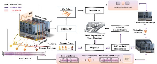
Figure 1: Overview of EvaGaussians. Our method seamlessly integrates the event streams captured by an event camera into the training of 3D-GS to robustly handle motion-blurred images. We adopt Event-based Double Integral (EDI) [28] for blur modeling and preprocessing, yielding initial camera trajectories and a sparse point cloud for 3D-GS training. By jointly optimizing the 3D-GS parameters and the camera motion trajectories using a blur reconstruction loss and an event reconstruction loss, our method facilitates high-quality 3D-GS reconstruction and novel view synthesis.

3.2 Modeling Motion-blurred Images Using Event Streams

The image formation process of digital cameras entails the accumulation of photons during the exposure time, which is then converted into electric charges. The motion-blurred images are resulted from camera movements during the exposure time. As introduced in [28], this phenomenon can be mathematically represented as follows:

$$\mathbf{B}=\frac{1}{\tau}\int_{f-\tau/2}^{f+\tau/2}\mathbf{I}(t)dt,$$ (4)

where $\mathbf{B}$ is the captured blurry image, which is equivalent to averaging the instantaneous latent images $\mathbf{I}(t)$ during the exposure time $[f-\tau/2,f+\tau/2]$. The optimization of 3D-GS requires camera calibration and point cloud initialization using COLMAP [35], which can fail when handling images with severe motion blur. To preliminarily obtain the camera poses and point clouds, we preprocess the motion-blurred images using the Event-based Double Integral (EDI) [28] model. Specifically, the EDI model is derived by substituting Eq. 3 into Eq. 4:

$$\mathbf{B}=\mathbf{I}(f)\cdot\frac{1}{\tau}\int_{f-\tau/2}^{f+\tau/2}\exp(c\,\mathbf{E}(t))dt.$$ (5)

Given the predefined threshold $c$, the captured blurry image $\mathbf{B}$, and the recorded event stream $\mathbf{E}(t)$, the EDI model (Eq. 5) allows the derivation of $\mathbf{I}(f)$, following which the latent image $\mathbf{I}(t)$ at any instance within the exposure time can be derived through Eq. 3. Then, as shown in Figure. 1, we uniformly sample $n$ time stamps during the exposure time and obtain a set of latent images that contains rich edge features, denoted as $\{\mathbf{I}_{i}\}_{i=0}^{n-1}$, and estimate their poses as well as obtain the initial point cloud of the scene using COLMAP [35]. Following this, a straightforward approach to optimize the 3D-GS is utilizing the preprocessed latent images as supervision. However, we found that this approach leads to poor reconstruction results, as the latent images, although providing more features than the original blurry image, still exhibits relatively low visual quality and also introduces inaccuracies into the estimated poses.

To more robustly recover a sharp 3D-GS from the motion-blurred images, we model the blurry image formation process using the EDI-produced camera poses and jointly optimize them with the 3D-GS parameters in a bundle adjustment manner [41]. Specifically, denote the estimated poses of each blurry view as $\{\mathbf{P}_{i}\}_{i=0}^{n-1}$, which roughly depicts the camera motion trajectory during the exposure time, we add each of them a learnable offset $\{\mathbf{d}_{i}\}_{i=0}^{n-1}$ as correction parameters. The resulting camera poses are defined as $\{\mathbf{\widetilde{P}}_{i}\}_{i=0}^{n-1}$, where $\mathbf{\widetilde{P}}_{i}=\mathbf{P}_{i}+\mathbf{d}_{i}$. During the optimization process, for each blurry view, we can simultaneously render $n$ images $\{\mathbf{\widetilde{I}}_{i}\}_{i=0}^{n-1}$ from the 3D-GS along the approximated camera trajectory, and simulate the formation of motion-blurred images using a discrete approximation of Eq 4, expressed as:

$$\mathbf{\widetilde{B}}=\frac{1}{n}\sum_{i=0}^{n-1}\mathbf{\widetilde{I}}_{i}.$$ (6)

For the total $K$ real captured blurry images $\{\mathbf{B}^{j}\}_{j=0}^{K-1}$, we can thus obtain their simulated versions $\{\mathbf{\widetilde{B}}^{j}\}_{j=0}^{K-1}$ through each learnable camera motion trajectory.

3.3 Loss Functions

Blur Reconstruction Loss. With the simulated blurry images, we use the real captured blurry images $\{\mathbf{B}^{j}\}_{j=0}^{K-1}$ to serve as image level supervision. Specifically, for each blurry image $\mathbf{B}^{j}$ and its simulated version $\mathbf{\widetilde{B}}^{j}$, we employ a blur reconstruction loss to minimize their photometric error, expressed as

$$\mathcal{L}_{blur}=(1-\lambda_{1})\cdot\|\mathbf{B}^{j}-\mathbf{\widetilde{B}}^{j}\|_{1}+\lambda_{1}\cdot\text{D-SSIM}(\mathbf{B}^{j},\mathbf{\widetilde{B}}^{j}).$$ (7)

The formation of blur reconstruction loss is the same as in the original 3D-GS [9], it differs in utilizing blurry images as supervision and jointly optimizing the 3D-GS parameters and the camera trajectories, thus facilitating an initial deblurring reconstruction of 3D-GS.

Event Reconstruction Loss. Leveraging the microsecond-level temporal resolution provided by the event streams, we further adopt an event reconstruction loss to aid in fine-grained deblurring. Specifically, we uniformly divide the exposure time into $m=n-1$ intervals, each with a length of $\frac{\tau}{m}$. Subsequently, we integrate the recorded event stream along these time intervals using Eq. 2, resulting in $m$ event maps $\{\mathbf{E}_{i}\}_{i=0}^{m-1}$ to serve as the event supervision. During training, for the $j$-th blurry view, we convert the rendered image sequence $\{\mathbf{\widetilde{I}}_{i}\}_{i=0}^{n-1}$ on the camera motion trajectory into event maps $\{\mathbf{\widetilde{E}}_{i}\}_{i=0}^{m-1}$, using a differentiable event simulator [31; 7], and constrain the discrepancies between the simulated event maps and the ground truth event maps, expressed as:

$$\mathcal{L}_{event}=\frac{1}{m}\sum_{i=0}^{m-1}\|\mathbf{E}_{i}-\mathbf{\widetilde{E}}_{i}\|_{1}.$$ (8)

The final loss function is the combination of the blur reconstruction loss and the event reconstruction loss, defined as:

$$\mathcal{L}=\lambda_{blur}\mathcal{L}_{blur}+\lambda_{event}\mathcal{L}_{event}.$$ (9)

During training, we jointly optimize the 3D-GS parameters and the camera motion trajectories using the defined loss function, ultimately achieving high-quality 3D-GS reconstruction from the captured blurry images and event streams.

3.4 Implementation Details.

We implemented EvaGaussians based on the official code of 3D-GS [9]. Throughout the training process, we set $\lambda_{1}=0.2$, $\lambda_{blur}=1$ and $\lambda_{event}=5\times{10}^{-3}$ for the loss function, and used $n=9$ for the number of poses to be optimized during the exposure time. In implementing the event reconstruction loss, we configured the positive threshold as ${c}_{pos}=0.25$ and the negative threshold as ${c}_{neg}=0.25$ for synthetic scenes, and set ${c}_{pos}=0.197$ and ${c}_{neg}=0.241$ for real scenes. The training process spans 50,000 iterations, with an event reconstruction loss introduced after a 3,000-iteration warmup. We execute 1,000 iterations to initialize the 3D-GS, after which we omit the densification process to streamline and simplify the subsequent optimization. All experiments were conducted using a single NVIDIA RTX 4090 GPU.

4 Experiments

4.1 Datasets.

Referring to [30; 3], we evaluate our method on both synthetic and real-world data. To ensure a comprehensive evaluation, we have contributed two novel datasets:

EvaGaussians-Blender Dataset. To evaluate the model’s ability to handle different scales of scenes, we construct a synthetic dataset covering a variety of scene scales, coupling with camera trajectories and event data. For large-scale scenes, we use Blender to design five diverse scenes, including city blocks and natural sceneries. For medium-scale scenes, we design three additional scenes using Blender, including classrooms, bedrooms, and cafes; we also redesign the camera trajectories of four scenes from DeblurNeRF [20]. For object-level scenes, we create six scenes based on the dataset from NeRF[23] and ${\textnormal{E}^{2}}$NeRF[30]. We simulate motion blur by manually placing multi-view cameras, randomly adjusting camera poses, and performing linear interpolation between the original and perturbed positions for each view. The images are rendered from these interpolated poses and blended in linear RGB space to produce the final blurred images. The corresponding event streams are generated using ESIM[31] and V2E[7]. The finally produced large-scale and medium-scale scenes include 35 views of blurred images and the corresponding event data, while the object-level scenes include 100 views of blurred images.

Table 1: Quantitative comparisons of novel view synthesis on large-scale scenes. The results are the average of 5 scenes, each with 100 views. We highlight the best-performing results in red and the second-best results in orange.

Novel View	B-NeRF	B-3DGS	UFP-GS	EDI-GS	EFN-GS	$\mathbf{E}^{2}$NeRF	BAD-NeRF	BAD-GS	EDNeRF	Ours
PSNR$\uparrow$	21.33	21.48	21.36	22.31	22.69	22.96	23.85	23.86	24.63	25.71
SSIM$\uparrow$	.6781	.6876	.6600	.6855	.6826	.7066	.7323	.7325	.7525	.7950
LPIPS$\downarrow$	.4249	.3971	.3736	.3823	.3631	.3751	.3480	.3473	.3279	.2745

Table 2: Quantitative comparisons of novel view synthesis on medium-scale scenes. The results are the average of 7 scenes, each with 100 views.

Novel View	B-NeRF	B-3DGS	UFP-GS	EDI-GS	EFN-GS	$\mathbf{E}^{2}$NeRF	BAD-NeRF	BAD-GS	EDNeRF	Ours
PSNR$\uparrow$	24.08	24.80	26.38	26.44	26.13	27.78	28.46	28.46	28.91	29.94
SSIM$\uparrow$	.7173	.7512	.8022	.8012	.7981	.8656	.8791	.8789	.8854	.9099
LPIPS$\downarrow$	.3617	.3187	.2639	.2581	.2726	.1985	.1823	.1816	.1692	.1551

Table 3: Quantitative comparisons of novel view synthesis for object-level Scenes. The results are the average of 6 objects, each with 100 views.

Novel View	B-NeRF	B-3DGS	UFP-GS	EDI-GS	EFN-GS	$\mathbf{E}^{2}$NeRF	BAD-NeRF	BAD-GS	EDNeRF	Ours
PSNR$\uparrow$	22.28	22.34	25.16	24.94	25.45	29.61	27.33	27.86	29.83	29.75
SSIM$\uparrow$	.9041	.9049	.9275	.9248	.9289	.9638	.9476	.9501	.9655	.9679
LPIPS$\downarrow$	.1479	.1471	.1174	.1208	.1103	.0735	.0928	.0911	.0722	.0714

EvaGaussians-DAVIS Dataset. The real-world experiments are performed on scenes captured by the Color DAVIS346 event camera [38]. It has a resolution of 346×260 pixels and we configured the exposure time for RGB frames at 100 milliseconds. We manually recorded five scenes, including three at the object level and two indoor scenes. The finally produced dataset consists of 30 images per scene coupled with the recorded event streams, each displaying various blur and lighting conditions. Please refer to Appendix. A for more details.

4.2 Experiment Settings

Baselines. We firstly compare our method with NeRF[23] and 3D-GS[9] directly trained on the blurry images, referring to them as Blurry-NeRF (B-NeRF) and Blurry-3DGS (B-3DGS). Then, we compare our method against several deblurring rendering methods, including ${\textnormal{E}^{2}}$NeRF[30], BAD-NeRF[41], BAD-Gaussians[48] (BAD-GS), and EvDeblurNeRF[3] (EDNeRF). Among these, the first two methods simulate motion blur and optimize camera trajectories without relying on event data, whereas the latter two are event-assisted methods. Additionally, we employ three image deblurring methods, namely UFP (a single-image deblurring method), EDI[28] (an event-based deblurring method) and EFNet[37] (a learnable event-based deblurring method), to process the input blurry images. Subsequently, we train vanilla 3D-GS using the deblurred images and name the resulting baselines UFP-GS, EDI-GS, EFN-GS.

Evaluation Metrics. We utilize a set of metrics to assess the performance of our model. For synthetic datasets, we employ three standard metrics: Peak Signal-to-Noise Ratio (PSNR), Structural Similarity Index Measure (SSIM) [42], and VGG-based Learned Perceptual Image Patch Similarity (LPIPS) [46]. These metrics serve to quantify the similarity between predicted novel views and provided target novel views. For real-world datasets, since the sharp ground-truth images are unavailable, we utilize a series of No-Reference Image Quality Assessment (NR-IQA) metrics to to evaluate our method. The adopted metrics include BRISQUE [24], NIQE [25], PIQE [40], RankIQA [18], and MetaIQA [50], which allow for effective evaluation when lacking ground truth images.

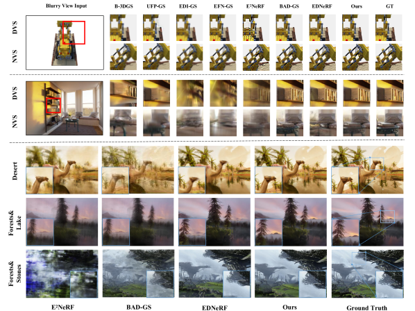
Figure 2: Qualitative comparision on the synthetic dataset. We show both novel view synthesis (NVS) results and input view deblurring (DVS) results on the top two rows. It shows that our method achieves better performance in recovering the training blurry views as well as rendering novel views. More results are presented in Appendix. B.

4.3 Synthetic Data Experiments

We evaluate our approach across a variety of scenes, including large-scale scenes, medium-scale scenes, and object-level scenes. Quantitative assessments of novel view synthesis are shown in Table. 1, Table. 2, and Table. 3, respectively. The deblurring results of input views are detailed in the Appendix. B. It can be found that our method achieves substantial improvements in most of the metrics, especially in challenging large scenes. Specifically, both B-NeRF and B-3DGS produce blurry novel views since they are directly trained on blurred images. The image deblurring-based baselines, UFP-GS, EDI-GS and EFN-GS, also produced inferior results, because the image deblurring process potentially corrupts the 3D consistency of the training images. Notably, our approach outperforms BAD-Gaussians[48] and BAD-NeRF[41], due to their limited capability in modeling complex textures. In addition, our method also surpasses the event-assisted methods ${\textnormal{E}^{2}}$NeRF[30] and EvDeblurNeRF[3] in producing high-quality novel views with intricate details, with better training and rendering efficiency. An extended analysis of all the baselines is provided in the Appendix. B.

The qualitative results are illustrated in Figure. 2. It is found that that although ${\textnormal{E}^{2}}$NeRF[30] performs well in object-level scenes, it struggles in medium and large-scale scene modeling, producing significant blurring results. Additionally, BAD-Gaussians[48] falls short in regions with pronounced color and depth variations, and produces overly smooth background textures. Although EvDeblurNeRF[3] exhibits overall satisfactory performance, its complex network architecture prolongs the training time (about 7 hours per scene) and precludes real-time rendering. In comparison, our method overcomes the baselines in producing high-fidelity novel views, and significantly reducing training time as well as demonstrating substantial advantages in real-time application scenarios. More visualization results are provided in Appendix. B.

Table 4: Quantitative comparisons of novel view synthesis on the real-world dataset. The table reports the average performance across five scenes. The results demonstrate that our method surpasses previous state-of-the-art approaches and achieves better performance across all metrics.

Novel View	B-NeRF	B-3DGS	UFP-GS	EDI-GS	EFN-GS	$\mathbf{E}^{2}$NeRF	BAD-NeRF	BAD-GS	EDNeRF	Ours
BRISQUE$\downarrow$	92.25	73.80	62.94	62.75	62.93	61.52	61.50	60.89	58.63	56.15
NIQE$\downarrow$	15.00	12.01	10.17	10.20	10.21	9.440	10.00	9.902	9.011	8.58
PIQE$\downarrow$	65.92	52.74	45.03	44.83	44.84	46.76	43.95	43.51	44.63	42.51
RankIQA$\downarrow$	9.428	7.542	6.439	6.411	6.411	5.573	6.285	6.223	5.320	5.067
MetaIQA$\uparrow$	.1241	.1418	.1732	.1737	.1737	.1809	.1773	.1790	.1909	.2009

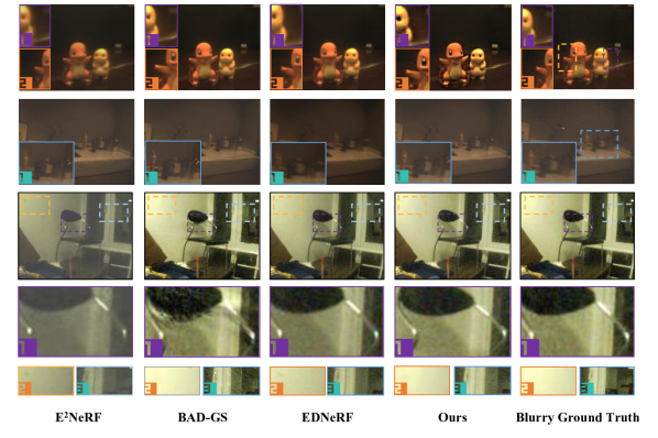
Figure 3: Qualitative results on the real-world dataset. It can be found that our method outperforms the baselines in synthesizing sharper novel views. More results are presented in Appendix. B.

4.4 Real-world Data Experiments

We present the quantitative results on the captured real-world data in Table. 4. It can be found that our method achieves superior performance compared to other approaches. Specifically, for NR-IQA metrics, we achieve improvements in BRISQUE, NIQE, PIQE, and RankIQA by 15.38%, 19.50%, 11.49%, and 22.83% respectively. We also achieve an increase in 19.38% in MetaIQA. The qualitative comparisons are illustrated in Figure. 3, which further demonstrate that our method is capable of reconstructing detailed textures, ultimately achieving higher-quality novel view synthesis. More results are presented in Appendix. B.

4.5 Ablation study

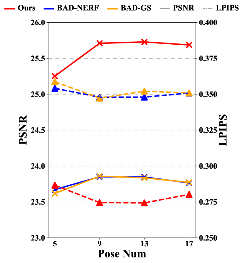
Figure 4: Ablation on number of poses in the camera trajectory.

Table 5: Quantitative ablation on $\mathcal{L}_{\text{event}}$ and $\mathcal{L}_{\text{blur}}$.

	w/o $\mathcal{L}_{\text{event}}\&\mathcal{L}_{\text{blur}}$	w/ $\mathcal{L}_{\text{blur}}$	w/ $\mathcal{L}_{\text{event}}\&\mathcal{L}_{\text{blur}}$
PSNR$\uparrow$	21.48	24.98	25.71
SSIM$\uparrow$	.6876	.7865	.7949
LPIPS$\downarrow$	.1222	.2986	.2745

Figure 5: Qualitative ablation on $\mathcal{L}_{\text{event}}$ and $\mathcal{L}_{\text{blur}}$.

Numbers of Camera Poses. We conduct ablations to investigate the effect of the number of camera poses optimized in the exposure time. We select five large scenes from our synthetic dataset for evaluation. In the experiments, we vary the number of camera poses, denoted as $n$, from 5, 9, 13, and 17. The quantitative results of the novel view rendering are displayed in Figure. 5. It indicates that the results reach a bottleneck at 9 poses. Beyond this point, the improvements are limited and may potentially lead to local convergence issues. Based on these experiments, we choose $n=9$ camera poses to achieve a balance between rendering performance and training efficiency. Here, we also provide comparison with BAD-NeRF [41] and BAD-Gaussians [48]. The two methods typically use linear interpolation to obtain camera trajectory, while our camera trajectories are estimated from the decomposed latent images, which provides more accurate initialization and helps our method achieves better performance.

Blur Reconstruction Loss and Event Reconstruction Loss. We conduct novel view synthesis experiments on five large-scale scenes from our synthetic dataset to validate the training losses. The quantitative results are reported in Table. 5, which indicate that the blurry reconstruction loss and event reconstruction loss significantly enhance novel view rendering quality. The qualitative ablation are shown in Figure. 5, where without the supervision of the proposed loss functions, the reconstruction results tends to produce oversmoothed results. With only the blur reconstruction loss, the produced results also lack high-frequency details. With the full losses, our method can produce high-fidelity novel views with intricate details.

5 Conclusions

This paper introduces Event Stream Assisted Gaussian Splatting (EvaGaussians), a novel framework that seamlessly integrates the event streams captured by an event camera into the training of 3D-GS, effectively addressing the challenges of reconstructing high-quality 3D-GS from motion-blurred images. We conducted comprehensive experiments on two novel datasets, and the results demonstrate that our method outperforms previous state-of-the-art deblurring rendering techniques. Despite its promising performance, our method may still face challenges when reconstructing scenes with extremely intricate textures from severely blurred images. We will release our code and dataset for future research.

Appendix A Datasets

A.1 Synthetic Data Generation

We created 9 medium-scale and large-scale raw scenes using Blender[4], utilizing these scenes in our experiments. Additionally, we remade and redesigned the camera trajectories for the cozyroom, factory, pool, and tanabata scenes from DeblurNeRF[19].

A.1.1 Introduction of the Synthetic Scenes

In this work, we utilized Blender to create a comprehensive dataset featuring a variety of indoor and outdoor scenes. These scenes are depicted in Figure. 6, and Figure. 7. The scenes created are meticulously crafted to provide a realistic and challenging environment for testing and training.

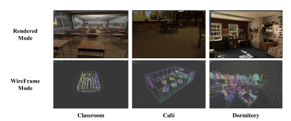
Figure 6: Visualization of EvaGaussians-Blender Indoor Scenes. The sizes of the Cafe and Classroom scenes are approximately ${15\times 7\times 4}$ meters, while the Dormitory scene is approximately ${5\times 5\times 4}$ meters (with an additional outdoor garden, making the overall scene size ${20\times 20\times 6}$ meters).

Indoor Scenes

• Classroom: A typical classroom setting featuring desks, chairs, a blackboard, and educational posters. This scene is designed to simulate an academic environment, ideal for educational and surveillance applications.

• Café: A cozy café with tables, chairs, a counter, and various decorations. This scene mimics a social setting, providing a dynamic backdrop for testing social interaction algorithms and retail analytics.

• Dormitory: A student dormitory room equipped with beds, study desks, personal belongings, and typical dorm furniture. This scene represents a personal living space, useful for smart home and security applications.

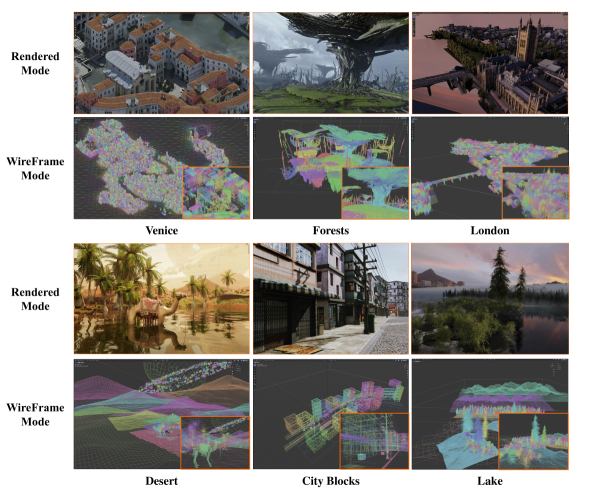
Figure 7: Visualization of EvaGaussians-Blender Outdoor Scenes. These scenes include rich details including skies, lakes, rivers, deserts, forests, stones, cities, roads, etc. All scenes cover an area of more than 1 square kilometer (relatively).

Outdoor Scenes

• Desert: A vast, arid landscape with sand dunes and sparse vegetation. This scene is perfect for testing navigation and object detection in harsh, unstructured environments.

• City Blocks: Urban scenes featuring streets, buildings, vehicles, and pedestrians. This environment is essential for autonomous driving, urban planning, and smart city applications.

• Lake: A serene natural setting with dense forests surrounding a tranquil lake. This scene provides a complex environment for testing outdoor navigation, environmental monitoring, and wildlife tracking.

• Forests: A rugged terrain with forested areas and scattered boulders. This scene is useful for off-road navigation and geological survey applications.

• Venice: A picturesque representation of Venice with canals, bridges, and historic architecture. This scene offers a unique setting for cultural heritage preservation, tourism, and urban analytics.

• London: A bustling cityscape of London with iconic landmarks, streets, and a dynamic urban environment. This scene supports applications in tourism, traffic management, and city modeling.

Our dataset aims to provide a wide range of realistic and diverse environments to facilitate the development and testing of advanced algorithms in various fields. Each scene is carefully crafted to ensure high-quality and detailed representations, making this dataset a valuable resource for researchers and developers.

A.1.2 Camera Trajectory in Blender

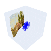
(a) Desert

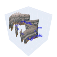
(b) Classroom

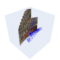
(c) Café

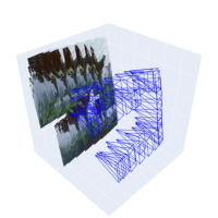
(d) Forests

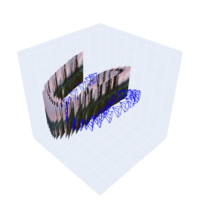
(e) Lake

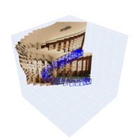
(f) Dormitory

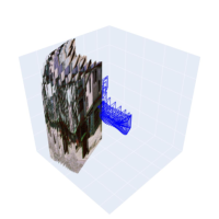
(g) City Blocks

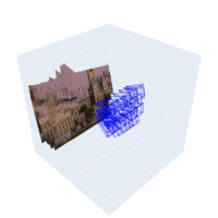
(h) London

Figure 8: Visualization of Camera Trajectory. The trajectories depicted were manually configured within Blender to ensure precise control over the camera paths. For the purpose of visualization and clarity, these trajectories have been normalized. This normalization process helps maintain consistent visibility and comparative analysis across different trajectory visualizations. Additionally, the normalization ensures that the visual representation accurately reflects the relative movements and orientations within the scene, providing a clear and comprehensive understanding of the camera dynamics throughout the depicted sequences.

A.1.3 Camera Settings

In our experiments conducted in Blender[4], we configured the virtual camera with a resolution of $400\times 600$ pixels for width and height, respectively, and set the scaling factor to 1.0. The virtual camera utilized a perspective model with a shutter speed of 1/180 seconds. Different focal lengths were employed for various scenes, and these parameters are documented in the corresponding data files.

A.1.4 Dataset Settings

We developed a dedicated script to generate motion blur and partition the dataset. Along a predefined virtual camera trajectory, we uniformly sampled 35 camera poses, adding a certain level of jitter to create the training set. We recorded the start and end times of the camera exposure, the positions, and the 20 intermediate frames during the exposure (obtained through linear interpolation between the start and end positions). We then uniformly sampled 100 camera poses along the same trajectory to form the test set. Using the event camera simulator from vid2e[7], we simulated the event data stream for the entire camera motion and synthesized the event bins from the events at the start and end of the exposure.

A.2 Real Data Capture

We use the Color DAVIS 346 event camera to record our real-time sequences and utilize the default camera settings provided in the DV software that comes with the camera.

A.2.1 Camera Calibration

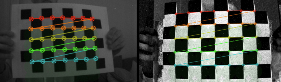
Figure 9: Visualization of Camera Calibration. Referencing [34], this figure illustrates the process and results of camera calibration using a checkerboard pattern. The left panel shows the checkerboard pattern captured from various positions and angles, with detected corner points utilized for calibration. The right panel presents the calibrated checkerboard pattern, demonstrating the corresponding points and lines between two cameras, which reflect the geometric relationship and accuracy achieved after calibration. Different colored lines indicate the correspondences between points during the calibration process.

We calibrated the event camera using the DV software provided by DAVIS. During the calibration process, we used a $6\times 9$ checkerboard pattern with a square size of 30 mm. In the software configuration, we set the width to 9, height to 6, and square size to 30 mm. We then ran the calibration module and moved the calibration pattern in front of the camera. The software detected the pattern and collected images, highlighting the detected area in green, as shown in Figure. 9. We set the minimum detections parameter to 50 to ensure a sufficient number of samples and used the consecutive detections parameter to ensure consistent pattern detection. Additionally, we enabled the image verification option to check the collected images in real-time, discarding inaccurately detected images and replacing them with new ones. We evaluate the calibration accuracy using the reprojection error $e_{r}$ as Eq. 10 and the epipolar error $e_{\text{epipolar}}$ as Eq. 11 in stereo calibration. The reprojection error is calculated as follows:

$$e_{r}=\frac{1}{n}\sum_{i=1}^{n}\|x_{i}-\hat{x}_{i}\|$$ (10)

where $x_{i}$ represents the observed points and $\hat{x}_{i}$ represents the projected points. The epipolar error is calculated as the average epipolar error for each point in all collected images. For each pair of images, the error is calculated as the sum of the distances between the points in one camera and the epipolar lines calculated from the other camera ($m$ is the number of acquired images, $n$ is the number of points). The formula is as follows:

$$e_{\text{epipolar}}=\frac{1}{m\times n}\sum_{i=1}^{m}\sum_{j=1}^{n}\left[d(P1_{i,j},l_{2,i,j})+d(P2_{i,j},l_{1,i,j})\right]$$ (11)

where $P1_{i,j}$ and $P2_{i,j}$ are the projection points of the $j$th point in the $i$th image in two cameras, and $l_{1,i,j}$ and $l_{2,i,j}$ are the epipolar lines corresponding to the $j$th point in the $i$th image calculated from the other camera. The maximum allowable error can be set under Max Reprojection Error. The stereo calibration also calculates the error caused by the epipolar constraint, which can be set under Max Epipolar Error. Once the calibration is successful, the results are saved and the undistorted output is displayed. The visualization results of the two types of errors are shown in Figure. 10. This process ensures the accuracy of the calibration, thereby improving the measurement accuracy and stability in subsequent applications.

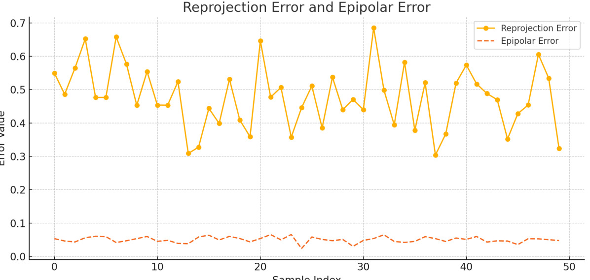
Figure 10: Visualization of Reprojection Errors and Epipolar Errors. The figure illustrates the 50 sets of reprojection errors and epipolar errors generated during the calibration process. The reprojection error $e_{r}$ represents the average discrepancy between the observed points and the projected points, calculated as shown in Equation equation 10. The epipolar error $e_{\text{epipolar}}$ represents the average distance between points in one camera and the epipolar lines calculated from the other camera for each pair of images, calculated as shown in Equation equation 11. As shown in the figure, the average reprojection error is approximately 0.5, and the average epipolar error is approximately 0.05, indicating a high level of accuracy in the calibration process.

A.2.2 Camera Settings

We recorded the five real scenes using the calibration parameters obtained during the calibration process. By adjusting the indoor lighting and shooting angles, we ensured the richness of the recorded scene details. The event camera thresholds were set according to its official documentation, with a contrast positive threshold $C_{p}=0.143$ and a contrast negative threshold $C_{n}=0.225$. Additionally, the camera has a spatial resolution of 346 × 260 pixels, a temporal resolution of 1 $\mu$s, a typical latency of less than 1 ms, a maximum throughput of 12 MEps, and a dynamic range of approximately 120 dB (with 50% of the pixels responding to 80% contrast changes under 0.1-100k lux conditions). The contrast sensitivity is 14.3% (ON) and 22.5% (OFF) (with 50% of the pixels responding). These parameters ensure that the event camera can stably and efficiently record scene information under various lighting conditions and dynamic ranges.

Appendix B Additional Experiment Results

To further validate the performance of our proposed model, we provide supplementary experimental results in this section. The following subsections offer a detailed analysis of the deblurring performance on the object-level scenes from the EvaGaussians-Blender dataset and present visualization results of novel views and deblurring views for each scene (Section. B.1). Additionally, we quantitatively analyze the deblurring performance and visualize the deblurring view and novel synthesis results in the medium-scale scenes (Section. B.2), and present quantitative comparisons for deblurring view synthesis (DVS) in the large-scale scenes (Section. B.3). Furthermore, in Section. B.4, we provide detailed evaluation metrics for each scene in the EvaGaussians-Blender dataset and visualize novel view synthesis (NVS) renderings of custom scenes in Section. B.5. Finally, we present evaluation metrics for each scene in the EvaGaussians-DAVIS dataset in Section. B.6.

B.1 Results of DVS in Object-level Scenes of EvaGaussians-Blender

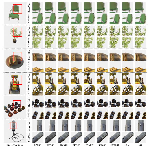
Figure 11: Visualization of DVS and NVS of Object-level Scenes in the EvaGaussian-Blender Dataset. It illustrates the performance of various methods in DVS and NVS tasks across multiple synthetic scenes. The results demonstrate that our method consistently excels in reconstructing fine details and maintaining high color accuracy compared to other methods. Notably, although our method performs less well in scenes with sparse elements such as $ficus,mic$, it shows superior performance in terms of visual fidelity and artifact reduction, closely matching the ground truth (GT) images.

In this section, we analyze the performance of our method in object-level scenes. Table. 6 and Figure. 11 present the quantitative and qualitative results of various methods across six synthetic scene sequences under default settings, which are optimal for all methods, as described in Section. 4.3. From the qualitative results, it is evident that our method excels in reconstructing fine details and maintaining high color accuracy in both deblurring view synthesis and novel view synthesis, as previously observed in Section. 4.3. In terms of quantitative results, our method outperforms baseline methods in most scenes and performs comparably in the remaining scenes. This is shown in the novel view synthesis results in Table 3 and the deblurring view synthesis results in Table 6.

Table 6: Quantitative comparisons of blur view synthesis for object-level scenes. The results presented in the table are the averages derived from six synthetic scenes from NeRF, utilizing 100 views in accordance with the ${\textnormal{E}^{2}}$NeRF[30] training process, and evaluate our method with sharp images of the same 100 views. We highlight the best-performing results in red and the second-best results in orange.

Novel View	B-NeRF	B-3DGS	UFP-GS	EDI-GS	EFN-GS	$\mathbf{E}^{2}$NeRF	BAD-NeRF	BAD-GS	EDNeRF	Ours
PSNR$\uparrow$	22.87	23.01	27.99	27.92	28.12	29.70	28.33	28.61	29.95	30.02
SSIM$\uparrow$	.9068	.9092	.9501	.9495	.9508	.9589	.9576	.9582	.9599	.9605
LPIPS$\downarrow$	.1450	.1437	.0743	.0747	.0739	.0722	.0734	.0732	.0720	.0719

B.2 Results of DVS in Medium-scale Scenes of EvaGaussians-Blender

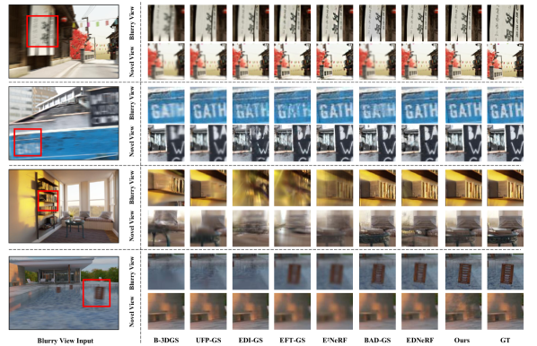
Figure 12: Visualization of DVS and NVS of Redesigned DeblurNeRF Scenes in the EvaGaussian-Blender Dataset. This figure showcases the performance of various methods in DVS and NVS tasks across multiple synthetic scenes. The results demonstrate that our method consistently excels in reconstructing fine details and maintaining high color accuracy compared to other methods. Notably, similar to object-level scenes, our method performs less effectively in highly reflective scenes such as pool. However, it still exhibits superior performance in terms of visual fidelity and artifact reduction, closely matching the ground truth (GT) images.

In this section, we present the quantitative deblurring results for medium-scale scenes, along with the visualization results of all models on the restructured DeblurNeRF dataset [19]. These experiments were conducted using the default parameters of each model. As shown in Table. 7, our method outperforms all others across all scenes. Additionally, Figure. 12 provides a detailed analysis of the deblurring and novel view synthesis results in the cozyroom, pool, factory, tanabata scenes which are medium scenes in the EvaGaussian-Blender Dataset. It can be observed that our model performs slightly worse than the NeRF baseline method in sky and water pool scenes. As noted in [48], the generalization performance of our model for transparent materials and sky scenes is inferior to the NeRF baseline method. However, our model excels in texture detail compared to other methods. These results demonstrate the superior learning capacity and generalization performance of our model.

Table 7: Quantitative comparisons of deblurring view synthesis on the medium-scale scenes of our EvaGaussians-Blender dataset. The table reports the average performance across four synthetic scenes, each trained utilizing 35 views and evaluate our method with sharp images of the same views. The results unequivocally demonstrate that our method surpasses previous state-of-the-art(SOTA) approaches, achieving superior performance consistently across all metrics.

Blur View	B-NeRF	B-3DGS	UFP-GS	EDI-GS	EFN-GS	$\mathbf{E}^{2}$NeRF	BAD-NeRF	BAD-GS	EDNeRF	Ours
PSNR$\uparrow$	24.27	25.05	26.60	26.65	26.30	27.95	28.62	28.70	29.12	30.26
SSIM$\uparrow$	.7254	.7631	.8135	.8100	.8068	.8743	.8883	.8890	.8951	.9241
LPIPS$\downarrow$	.3513	.3101	.2547	.2486	.2628	.1874	.1735	.1715	.1588	.1419

B.3 Results of DVS in Large-scale Scenes of EvaGaussians-Blender

As a supplement to the synthetic experiments detailed in Section. 4.3, we also performed experiments on deblurring view synthesis using the same experimental setup. The results are presented in Table. 8. Consistent with the findings in Section. B.1, these results further confirm the effectiveness of our model. Additionally, the per-scene breakdown of the EvaGaussians-Blender Dataset results is shown in Table. 9, Table. 10, and Table. 11. Similar to the deblurring view synthesis results, our method consistently achieves the best performance across all scenes.

Table 8: Quantitative comparison of deblurring view synthesis on the large-scale scenes in our EvaGaussians-Blender dataset. The table reports the average performance across four synthetic scenes, each trained utilizing 35 views and evaluate our method with sharp images of the same views. The results unequivocally demonstrate that our method surpasses previous SOTA approaches, achieving superior performance consistently across all metrics.

Novel View	B-NeRF	B-3DGS	UFP-GS	EDI-GS	EFN-GS	$\mathbf{E}^{2}$NeRF	BAD-NeRF	BAD-GS	EDNeRF	Ours
PSNR$\uparrow$	21.42	21.58	21.43	22.36	22.75	23.02	23.92	23.98	24.79	25.85
SSIM$\uparrow$	.6795	.6914	.6690	.6943	.6915	.7155	.7412	.7425	.7614	.8039
LPIPS$\downarrow$	.4185	.3860	.3672	.3710	.3520	.3689	.3468	.3459	.3168	.2635

B.4 Per-scene Breakdown for Novel View Synthesis in Medium and Large Scale Scenes

In this subsection, we present a detailed analysis of the novel view synthesis performance in medium and large scale scenes from the EvaGaussians-Blender dataset. Table. 9 summarizes the Peak Signal-to-Noise Ratio results and the NVS results demonstrate that our proposed method consistently outperforms other approaches across various scenes. Specifically, our model achieves superior PSNR values, indicating higher reconstruction quality and better visual fidelity. The detailed metrics for Structural Similarity Index and Learned Perceptual Image Patch Similarity further corroborate these findings in Table. 10 and Table. 11, showing that our model excels in maintaining structural integrity and perceptual quality in synthesized views.

In medium-scale scenes, our method exhibits robust performance, particularly in complex environments where maintaining detail and minimizing artifacts are challenging. This robustness is evident in scenes such as cozyroom and factory, where our method achieves significant improvements in both PSNR and SSIM, reflecting enhanced clarity and texture detail. For large-scale scenes, our model continues to demonstrate its efficacy, especially in handling large areas and diverse visual features. Scenes like desert and city blocks highlight the model’s capability to generalize across different scales, providing high-quality novel view synthesis with minimal perceptual discrepancies. These comprehensive results underscore the advanced learning and generalization capabilities of our model, setting a new benchmark for novel view synthesis in medium- and large-scale scenes.

Table 9: The Novel View Synthesis Results of PSNR $\uparrow$ in the EvaGaussians-Blender Dataset. The highest values in each category are highlighted in bold to indicate the best results.

Models	Medium							Large
	Classroom	Dormitory	Café	Pool	Cozyroom	Factory	Tanabata	Desert	City Blocks	London	Forests	Lake
Blurry-NeRF	25.42	26.72	21.23	26.66	15.42	26.76	26.38	19.04	19.34	20.00	23.60	24.67
Blurry-GS	25.59	26.83	21.34	26.17	20.76	26.48	26.46	19.67	19.48	20.18	23.75	24.34
UFP-GS	28.64	29.68	21.54	26.79	21.62	27.60	28.77	20.78	20.85	16.61	22.96	25.60
EDI-GS	28.49	29.90	22.62	26.36	21.17	29.06	27.46	20.66	20.68	20.27	23.97	25.99
EFNET-GS	28.59	29.48	22.04	26.36	21.42	27.57	27.43	20.62	21.70	20.36	25.57	25.18
$\textnormal{E}^{2}$NeRF	28.87	30.77	26.16	28.92	21.23	29.85	28.65	20.02	21.78	21.30	25.90	25.78
BAD-NeRF	30.28	31.23	27.18	28.71	21.68	30.28	29.85	21.09	21.91	22.91	26.35	26.99
BAD-Gaussians	30.28	31.23	27.18	28.72	21.68	30.28	29.85	21.10	21.93	22.93	26.35	26.98
EvDeblurNeRF	31.83	28.95	28.66	29.69	22.01	31.20	30.02	21.62	22.23	23.88	27.10	28.29
Ours	33.62	32.19	29.71	30.05	22.52	31.38	30.14	24.65	23.56	23.58	27.41	29.35

Table 10: The Novel View Synthesis of SSIM $\uparrow$ in the EvaGaussians-Blender Dataset. The highest values in each category are highlighted in bold to indicate the best results.

Models	Medium							Large
	Classroom	Dormitory	Café	Pool	Cozyroom	Factory	Tanabata	Desert	City Blocks	London	Forests	Lake
Blurry-NeRF	0.7086	0.8281	0.5682	0.7442	0.5098	0.8567	0.8057	0.6023	0.6325	0.6732	0.7002	0.7823
Blurry-GS	0.7154	0.8312	0.5638	0.7265	0.7632	0.8519	0.8064	0.6386	0.6341	0.6819	0.7026	0.7807
UFP-GS	0.8701	0.9281	0.5706	0.7527	0.7729	0.8640	0.8569	0.6172	0.6144	0.5807	0.6911	0.7968
EDI-GS	0.8456	0.9291	0.5977	0.7288	0.7703	0.8963	0.8408	0.6567	0.5655	0.6882	0.7158	0.8012
EFNET-GS	0.8692	0.9259	0.5841	0.7288	0.7797	0.8643	0.8345	0.6164	0.6366	0.6069	0.7628	0.7901
$\textnormal{E}^{2}$NeRF	0.8723	0.9319	0.7869	0.8795	0.7724	0.9245	0.8915	0.6169	0.6822	0.6734	0.7467	0.8139
BAD-NeRF	0.8978	0.9337	0.8041	0.8794	0.7764	0.9353	0.9271	0.6314	0.6867	0.6932	0.7583	0.8919
BAD-Gaussians	0.8992	0.9351	0.8031	0.8781	0.7755	0.9345	0.9266	0.6346	0.6851	0.6944	0.7578	0.8908
EvDeblurNeRF	0.9023	0.8935	0.8513	0.8885	0.7854	0.9454	0.9311	0.6589	0.7023	0.7159	0.7726	0.9129
Ours	0.9334	0.9545	0.8981	0.8973	0.8015	0.9494	0.9348	0.8093	0.7347	0.7015	0.7988	0.9306

Table 11: The Novel View Synthesis of LPIPS $\downarrow$ in the EvaGaussians-Blender Dataset. The highest values in each category are highlighted in bold to indicate the best results.

Models	Medium							Large
	Classroom	Dormitory	Café	Pool	Cozyroom	Factory	Tanabata	Desert	City Blocks	London	Forests	Lake
Blurry-NeRF	0.3987	0.2998	0.4528	0.3848	0.5545	0.2063	0.2348	0.4447	0.5273	0.3971	0.3425	0.4127
Blurry-GS	0.3824	0.2873	0.4554	0.4198	0.2432	0.2091	0.2335	0.4231	0.4116	0.3925	0.3379	0.4206
UFP-GS	0.2838	0.1361	0.4511	0.3646	0.2331	0.1928	0.1856	0.3816	0.3342	0.4069	0.3383	0.4069
EDI-GS	0.2914	0.1267	0.4038	0.4102	0.2388	0.1446	0.1911	0.4062	0.3857	0.3901	0.3295	0.4001
EFNET-GS	0.2846	0.1373	0.4529	0.4102	0.2345	0.1926	0.1958	0.3912	0.3222	0.3932	0.2962	0.4128
$\textnormal{E}^{2}$NeRF	0.2821	0.1165	0.2871	0.2048	0.2369	0.1073	0.1546	0.3938	0.3713	0.3928	0.3589	0.3588
BAD-NeRF	0.2365	0.1083	0.2715	0.2103	0.2278	0.0992	0.1224	0.3947	0.3618	0.3224	0.3467	0.3142
BAD-Gaussians	0.2384	0.1078	0.2695	0.2094	0.2262	0.0985	0.1215	0.3965	0.3604	0.3215	0.3452	0.3129
EvDeblurNeRF	0.2217	0.1455	0.2447	0.1926	0.1942	0.0768	0.1086	0.3823	0.3497	0.2972	0.3163	0.2941
Ours	0.1981	0.0948	0.2328	0.1889	0.1920	0.0756	0.1037	0.2156	0.2862	0.3092	0.2924	0.2691

B.5 Visualization of Qualitative Results for NVS in EvaGaussians-Blender Datasets

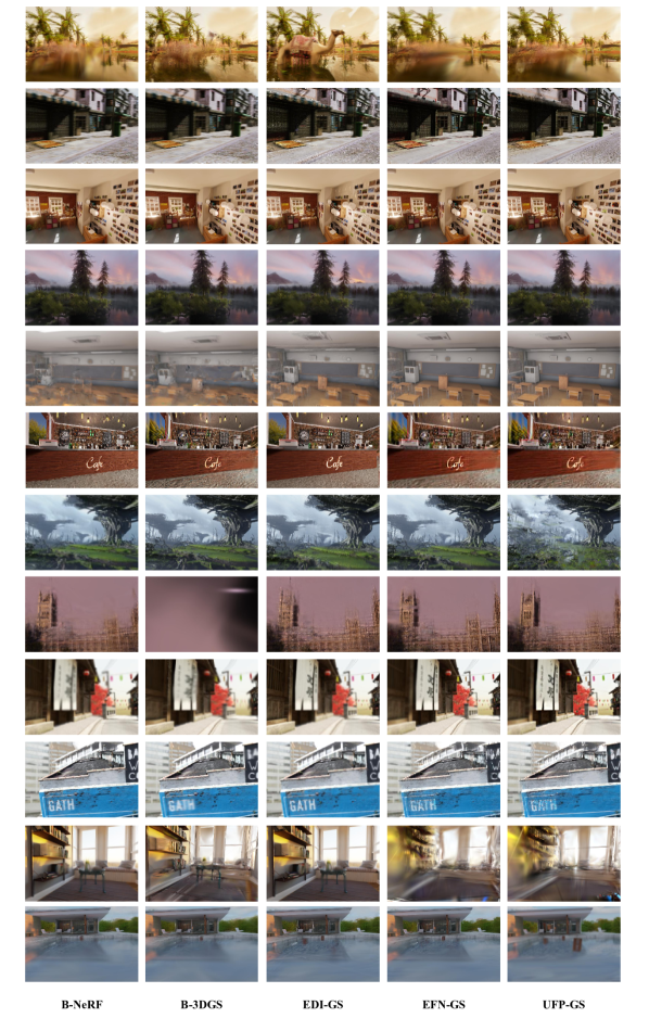
Figure 13: Visualization of Novel View Synthesis of All-redesigned Scenes with B-NeRF, B-3DGS, EDI-GS, EFN-GS and UFP-GS in the EvaGaussian-Blender Dataset.

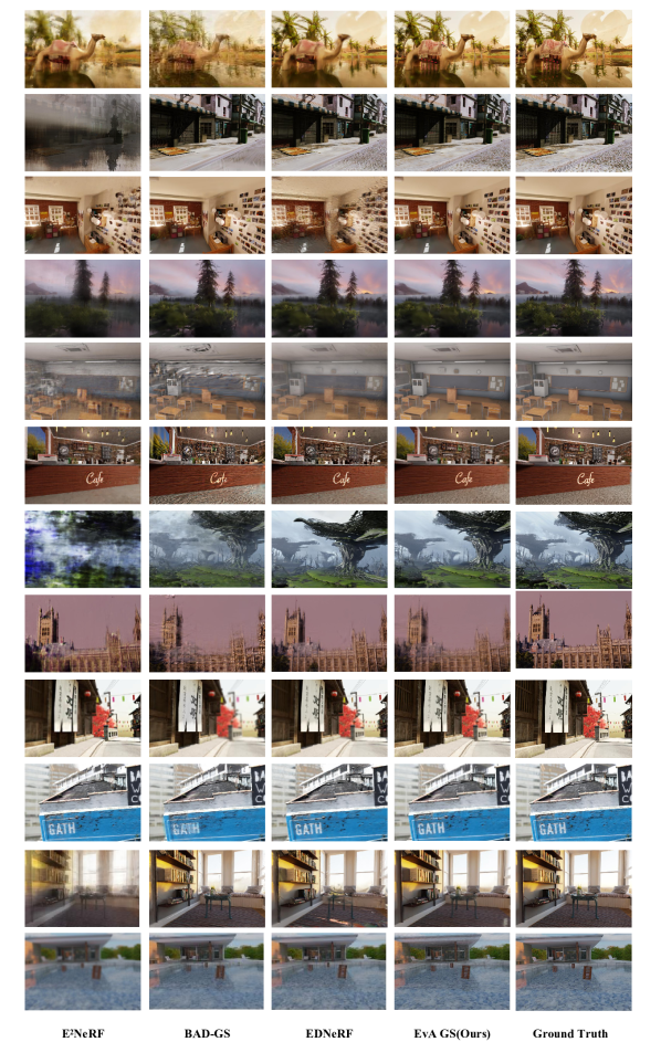
Figure 14: Visualization of Novel View Synthesis of All-redesigned Scenes with ${\textnormal{E}^{2}}$NeRF, BAD-GS, EDNeRF and EvAGS in the EvaGaussian-Blender Dataset.

In this section, we present the qualitative results of novel view synthesis for custom scenes in the EvaGaussians-Blender dataset, such as desert and city blocks. These visualizations highlight our model’s ability to reconstruct fine details and maintain high color accuracy. By comparing our method with baseline approaches, we demonstrate the visual fidelity and robustness of our model across different scenes under the same experimental settings. The synthesized views shown in Figure. 13 and Figure.  14 further exemplify the superior performance of our method in terms of detail preservation and color consistency.

B.6 Results of Deblurring and Novel View Synthesis in EvaGaussians-DAVIS Datasets

In this section, we present a comprehensive analysis of the deblurring and novel view synthesis results on the EvaGaussians-DAVIS dataset. The evaluation metrics include BRISQUE, NIQE, PIQE, MetaIQA, and RankIQA, which quantitatively assess the quality of synthesized views across different scenes such as desk & chair, washroom, pokémon, pillow, and bag.

Our method consistently achieves the lowest BRISQUE, NIQE, and PIQE scores, indicating superior perceptual quality in the synthesized views. Specifically, as shown in Table. 12, our model achieves the best BRISQUE scores across all scenes, highlighting its ability to produce visually appealing and less distorted images.

For NIQE, as presented in Table. 13, our approach significantly outperforms the baselines, achieving the lowest average NIQE score. This demonstrates our method’s robustness in generating high-quality images with minimal perceptual artifacts, further confirmed by its performance across individual scenes.

In terms of PIQE, Table. 14 shows that our model again leads in performance, achieving the lowest PIQE scores, which correlates with higher perceived image quality. This underscores the effectiveness of our model in preserving image details and reducing noise.

Furthermore, our method excels in MetaIQA and RankIQA evaluations, as detailed in Tables. 15 and Table. 16, respectively. The highest MetaIQA scores and lowest RankIQA scores across most scenes affirm the overall superior visual quality and fidelity of our synthesized views compared to baseline models.

Overall, these results demonstrate the advanced learning capabilities and generalization performance of our model, particularly in handling complex scenes and maintaining high visual quality across diverse scenarios. The consistent performance across multiple evaluation metrics solidifies our approach as a leading solution for novel view synthesis in realistic environments.

Table 12: The Novel View Synthesis of BRISQUE in the EvaGaussians-DAVIS Dataset. The highest values in each category are highlighted in bold to indicate the best results.

Models	BRISQUE $\downarrow$
	Desk & Chair	Washroom	Pokémon	Pillow	Bag	Average
B-NeRF	63.9428	102.7828	109.2711	97.4778	87.7699	92.2489
B-3DGS	51.1542	82.2262	87.4169	77.9823	70.2159	73.7991
UFP-GS	43.6932	69.7354	74.6684	66.6098	59.9711	62.9356
EDI-GS	43.4811	69.9923	74.3044	66.2849	59.6835	62.7492
EFN-GS	43.5235	69.8473	74.2875	66.3158	59.6523	62.7253
${\textnormal{E}^{2}}$NeRF	36.2148	64.4332	77.0112	67.1324	62.8063	61.5196
BAD-NeRF	42.6285	68.5219	72.8474	64.9852	58.5133	61.4993
BAD-GS	42.2065	67.8434	72.1261	64.3418	57.9339	60.8903
EDNeRF	34.5687	61.5044	73.5012	64.0809	59.4969	58.6304
Ours	32.9225	58.5756	70.0211	61.0294	58.1876	56.1472

Table 13: The Novel View Synthesis of NIQE in the EvaGaussians-DAVIS Dataset.

Models	NIQE $\downarrow$
	Desk & Chair	Washroom	Pokémon	Pillow	Bag	Average
B-NeRF	11.4380	15.5386	16.9153	16.2316	14.8844	15.0016
B-3DGS	9.1504	12.4309	13.5323	12.9853	11.9075	12.0113
UFP-GS	7.7736	10.6170	11.3827	10.9266	10.1715	10.1743
EDI-GS	7.7778	10.5662	11.5024	11.0375	10.1214	10.2011
EFN-GS	7.8235	10.5412	11.4868	11.0743	10.1288	10.2109
${\textnormal{E}^{2}}$NeRF	6.8907	9.0924	11.6383	10.1830	9.3954	9.4400
BAD-NeRF	7.6253	10.3590	11.2769	10.8211	9.9229	10.0011
BAD-GS	7.5498	10.2565	11.1652	10.7139	9.8247	9.9020
EDNeRF	6.5775	8.6791	11.1092	9.7201	8.9684	9.0109
Ours	6.2643	8.2658	10.5802	9.2573	8.5413	8.5818

Table 14: The Novel View Synthesis of PIQE in the EvaGaussians-DAVIS Dataset.

Models	PIQE $\downarrow$
	Desk & Chair	Washroom	Pokémon	Pillow	Bag	Average
B-NeRF	58.4566	68.8701	73.4701	54.0862	74.7257	65.9217
B-3DGS	46.7653	55.0961	58.7761	43.2689	59.7806	52.7374
UFP-GS	39.9453	47.0612	50.2026	36.9659	50.9631	45.0276
EDI-GS	39.7505	46.8317	49.9597	36.7786	50.8135	44.8268
EFN-GS	39.7748	46.7951	49.9346	36.7891	50.8275	44.8242
${\textnormal{E}^{2}}$NeRF	40.9825	49.2988	50.4868	39.7896	53.2203	46.7556
BAD-NeRF	38.9711	45.9134	48.9801	36.0574	49.8171	43.9478
BAD-GS	38.5852	45.4588	48.4951	35.7004	49.3239	43.5127
EDNeRF	39.1197	47.0580	48.1919	37.9810	50.8012	44.6304
Ours	37.2568	44.8171	45.8971	36.1724	48.3821	42.5051

Table 15: The Novel View Synthesis of MetaIQA in the EvaGaussians-DAVIS Dataset.

Models	MetaIQA $\uparrow$
	Desk & Chair	Washroom	Pokémon	Pillow	Bag	Average
B-NeRF	0.1419	0.1272	0.1085	0.1122	0.1307	0.1241
B-3DGS	0.1621	0.1454	0.1240	0.1283	0.1494	0.1418
UFP-GS	0.1976	0.1774	0.1521	0.1564	0.1823	0.1732
EDI-GS	0.1986	0.1780	0.1518	0.1571	0.1830	0.1737
EFN-GS	0.1928	0.1835	0.1579	0.1643	0.1799	0.1757
${\textnormal{E}^{2}}$NeRF	0.1959	0.2020	0.1619	0.1723	0.1722	0.1809
BAD-NeRF	0.2027	0.1817	0.1549	0.1603	0.1867	0.1773
BAD-GS	0.2047	0.1835	0.1565	0.1620	0.1886	0.1790
EDNeRF	0.2067	0.2132	0.1709	0.1819	0.1817	0.1909
Ours	0.2176	0.2245	0.1799	0.1915	0.1913	0.2009

Table 16: The Novel View Synthesis of RankIQA in the EvaGaussians-DAVIS Dataset.

Models	RankIQA $\downarrow$
	Desk & Chair	Washroom	Pokémon	Pillow	Bag	Average
B-NeRF	7.4896	10.4454	10.7921	9.6578	8.7541	9.4278
B-3DGS	5.9917	8.3563	8.6337	7.7262	7.0032	7.5422
UFP-GS	5.1153	7.1215	7.3741	6.6005	5.9829	6.4389
EDI-GS	5.0929	7.1029	7.3386	6.5673	5.9528	6.4109
EFN-GS	5.1046	7.0893	7.3158	6.5789	5.9682	6.4114
${\textnormal{E}^{2}}$NeRF	4.5141	6.4997	5.7764	5.7600	5.3166	5.5733
BAD-NeRF	4.9931	6.9636	7.1948	6.4385	5.8360	6.2852
BAD-GS	4.9436	6.8947	7.1235	6.3748	5.7783	6.2230
EDNeRF	4.3089	6.2043	5.5138	5.4981	5.0749	5.3200
Ours	4.1037	5.9088	5.2513	5.2363	4.8332	5.0667

Appendix C Broader Impact

Our proposed EvaGaussians utilizes event cameras to perform 3D-reconstruction from low-quality, blurred images. It has the potential to bring about both positive and negative societal impacts.

On the positive side, our method can improve the efficiency of surveillance systems by reconstructing clear 3D images from low-quality footage, enabling better identification of individuals and objects in challenging conditions. This can bolster public safety and aid in criminal investigations. Additionally, the ability to reconstruct scenes from blurred inputs can enhance the performance of autonomous vehicles, drones, and robots, enabling them to navigate more accurately in poor visibility conditions, leading to safer and more efficient transportation and logistics. In situations where traditional cameras may struggle to capture clear images under extreme conditions, our method can provide valuable information for first responders and rescue teams, helping them make informed decisions and potentially saving lives. Furthermore, our technique can be applied to medical imaging, allowing for better visualization of internal structures and more accurate diagnoses, ultimately leading to improved patient outcomes.

On the negative side, the enhanced surveillance capabilities enabled by our method may raise privacy concerns. For example, our method could be used for malicious purposes, such as stalking or spying on individuals without their consent. It is important to establish regulations and guidelines to prevent such misuse.

References

- [1] Patrick Bardow, Andrew J Davison, and Stefan Leutenegger. Simultaneous optical flow and intensity estimation from an event camera. In Computer Vision and Pattern Recognition (CVPR), 2016.
- [2] Marco Cannici and Davide Scaramuzza. Mitigating motion blur in neural radiance fields with events and frames. In Computer Vision and Pattern Recognition (CVPR), 2024.
- [3] Marco Cannici and Davide Scaramuzza. Mitigating motion blur in neural radiance fields with events and frames. In Proceedings of the IEEE/CVF Conference on Computer Vision and Pattern Recognition (CVPR), 2024.
- [4] Blender Online Community. Blender - a 3D modelling and rendering package. Blender Foundation, Stichting Blender Foundation, Amsterdam, 2018.
- [5] Guillermo Gallego, Tobi Delbrück, Garrick Orchard, Chiara Bartolozzi, Brian Taba, Andrea Censi, Stefan Leutenegger, Andrew J Davison, Jörg Conradt, Kostas Daniilidis, et al. Event-based vision: A survey. IEEE Trans. Pattern Analysis and Machine Intelligence (PAMI), 2020.
- [6] Mathias Gehrig and Davide Scaramuzza. Recurrent vision transformers for object detection with event cameras. In Computer Vision and Pattern Recognition (CVPR), 2023.
- [7] Yuhuang Hu, Shih-Chii Liu, and Tobi Delbruck. v2e: From video frames to realistic dvs events. In Proceedings of the IEEE/CVF Conference on Computer Vision and Pattern Recognition, pages 1312–1321, 2021.
- [8] Zhe Jiang, Yu Zhang, Dongqing Zou, Jimmy Ren, Jiancheng Lv, and Yebin Liu. Learning event-based motion deblurring. In Computer Vision and Pattern Recognition (CVPR), 2020.
- [9] Bernhard Kerbl, Georgios Kopanas, Thomas Leimkühler, and George Drettakis. 3d gaussian splatting for real-time radiance field rendering. ACM Transactions on Graphics (TOG), 2023.
- [10] Justin Kerr, Chung Min Kim, Ken Goldberg, Angjoo Kanazawa, and Matthew Tancik. Lerf: Language embedded radiance fields. In Computer Vision and Pattern Recognition (CVPR), 2023.
- [11] Joseph J LaViola Jr. Bringing vr and spatial 3d interaction to the masses through video games. IEEE Computer Graphics and Applications, 2008.
- [12] Dogyoon Lee, Minhyeok Lee, Chajin Shin, and Sangyoun Lee. Dp-nerf: Deblurred neural radiance field with physical scene priors. In Computer Vision and Pattern Recognition (CVPR), 2023.
- [13] Marc Levoy. Efficient ray tracing of volume data. ACM Transactions on Graphics (TOG), 1990.
- [14] Chenghan Li, Christian Brandli, Raphael Berner, Hongjie Liu, Minhao Yang, Shih-Chii Liu, and Tobi Delbruck. Design of an rgbw color vga rolling and global shutter dynamic and active-pixel vision sensor. In IEEE International Symposium on Circuits and Systems (ISCAS), 2015.
- [15] Songnan Lin, Jiawei Zhang, Jinshan Pan, Zhe Jiang, Dongqing Zou, Yongtian Wang, Jing Chen, and Jimmy Ren. Learning event-driven video deblurring and interpolation. In European Conference on Computer Vision (ECCV), 2020.
- [16] Kunhao Liu, Fangneng Zhan, Jiahui Zhang, Muyu Xu, Yingchen Yu, Abdulmotaleb El Saddik, Christian Theobalt, Eric Xing, and Shijian Lu. Weakly supervised 3d open-vocabulary segmentation. In Neural Information Processing Systems (NIPS), 2023.
- [17] Minghua Liu, Ruoxi Shi, Kaiming Kuang, Yinhao Zhu, Xuanlin Li, Shizhong Han, Hong Cai, Fatih Porikli, and Hao Su. Openshape: Scaling up 3d shape representation towards open-world understanding. In Neural Information Processing Systems (NIPS), 2024.
- [18] Xialei Liu, Joost Van De Weijer, and Andrew D Bagdanov. Rankiqa: Learning from rankings for no-reference image quality assessment. In Proceedings of the IEEE international conference on computer vision, pages 1040–1049, 2017.
- [19] Li Ma, Xiaoyu Li, Jing Liao, Qi Zhang, Xuan Wang, Jue Wang, and Pedro V Sander. Deblur-NeRF: Neural Radiance Fields from Blurry Images. In Computer Vision and Pattern Recognition (CVPR), 2022.
- [20] Li Ma, Xiaoyu Li, Jing Liao, Qi Zhang, Xuan Wang, Jue Wang, and Pedro V Sander. Deblur-nerf: Neural radiance fields from blurry images. In Proceedings of the IEEE/CVF Conference on Computer Vision and Pattern Recognition, pages 12861–12870, 2022.
- [21] Nelson Max. Optical models for direct volume rendering. ACM Transactions on Graphics (TOG), 1995.
- [22] Nico Messikommer, Carter Fang, Mathias Gehrig, and Davide Scaramuzza. Data-driven feature tracking for event cameras. In Computer Vision and Pattern Recognition (CVPR), 2023.
- [23] Ben Mildenhall, Pratul P Srinivasan, Matthew Tancik, Jonathan T Barron, Ravi Ramamoorthi, and Ren Ng. NeRF: Representing Scenes as Neural Radiance Fields for View Synthesis. In European Conference on Computer Vision (ECCV), 2020.
- [24] Anish Mittal, Anush Krishna Moorthy, and Alan Conrad Bovik. No-reference image quality assessment in the spatial domain. IEEE Trans. on Image Processing (TIP), 21(12):4695–4708, 2012.
- [25] Anish Mittal, Rajiv Soundararajan, and Alan C Bovik. Making a “completely blind” image quality analyzer. IEEE Signal processing letters, 20(3):209–212, 2012.
- [26] Genady Paikin, Yotam Ater, Roy Shaul, and Evgeny Soloveichik. Efi-net: Video frame interpolation from fusion of events and frames. In Computer Vision and Pattern Recognition (CVPR), 2021.
- [27] Liyuan Pan, Miaomiao Liu, and Richard Hartley. Single image optical flow estimation with an event camera. In Computer Vision and Pattern Recognition (CVPR), 2020.
- [28] Liyuan Pan, Cedric Scheerlinck, Xin Yu, Richard Hartley, Miaomiao Liu, and Yuchao Dai. Bringing a blurry frame alive at high frame-rate with an event camera. In Computer Vision and Pattern Recognition (CVPR), 2019.
- [29] Etienne Perot, Pierre De Tournemire, Davide Nitti, Jonathan Masci, and Amos Sironi. Learning to detect objects with a 1 megapixel event camera. In Neural Information Processing Systems (NIPS), 2020.
- [30] Yunshan Qi, Lin Zhu, Yu Zhang, and Jia Li. E2nerf: Event enhanced neural radiance fields from blurry images. In International Conference on Computer Vision (ICCV), 2023.
- [31] Henri Rebecq, Daniel Gehrig, and Davide Scaramuzza. Esim: an open event camera simulator. In Conference on robot learning, pages 969–982. PMLR, 2018.
- [32] Henri Rebecq, René Ranftl, Vladlen Koltun, and Davide Scaramuzza. High speed and high dynamic range video with an event camera. IEEE Trans. Pattern Analysis and Machine Intelligence (PAMI), 2019.
- [33] Antoni Rosinol, John J Leonard, and Luca Carlone. Nerf-slam: Real-time dense monocular slam with neural radiance fields. In International Conference on Intelligent Robots and Systems (IROS), 2023.
- [34] Viktor Rudnev, Mohamed Elgharib, Christian Theobalt, and Vladislav Golyanik. Eventnerf: Neural radiance fields from a single colour event camera. In Computer Vision and Pattern Recognition (CVPR), 2023.
- [35] Johannes L Schonberger and Jan-Michael Frahm. Structure-from-motion Revisited. In Computer Vision and Pattern Recognition (CVPR), 2016.
- [36] Lei Sun, Christos Sakaridis, Jingyun Liang, Qi Jiang, Kailun Yang, Peng Sun, Yaozu Ye, Kaiwei Wang, and Luc Van Gool. Event-based fusion for motion deblurring with cross-modal attention. In European Conference on Computer Vision (ECCV).
- [37] Lei Sun, Christos Sakaridis, Jingyun Liang, Qi Jiang, Kailun Yang, Peng Sun, Yaozu Ye, Kaiwei Wang, and Luc Van Gool. Event-based fusion for motion deblurring with cross-modal attention. In European Conference on Computer Vision, pages 412–428. Springer, 2022.
- [38] Gemma Taverni. Applications of Silicon Retinas: From Neuroscience to Computer Vision. PhD thesis, Universität Zürich, 2020.
- [39] Stepan Tulyakov, Daniel Gehrig, Stamatios Georgoulis, Julius Erbach, Mathias Gehrig, Yuanyou Li, and Davide Scaramuzza. Time lens: Event-based video frame interpolation. In Computer Vision and Pattern Recognition (CVPR), pages 16155–16164, 2021.
- [40] N Venkatanath, D Praneeth, Maruthi Chandrasekhar Bh, Sumohana S Channappayya, and Swarup S Medasani. Blind image quality evaluation using perception based features. In 2015 twenty first national conference on communications (NCC), pages 1–6. IEEE, 2015.
- [41] Peng Wang, Lingzhe Zhao, Ruijie Ma, and Peidong Liu. BAD-NeRF: Bundle Adjusted Deblur Neural Radiance Fields. In Computer Vision and Pattern Recognition (CVPR), 2023.
- [42] Zhou Wang, Alan C Bovik, Hamid R Sheikh, and Eero P Simoncelli. Image quality assessment: from error visibility to structural similarity. IEEE transactions on image processing, 13(4):600–612, 2004.
- [43] Linning Xu, Vasu Agrawal, William Laney, Tony Garcia, Aayush Bansal, Changil Kim, Samuel Rota Bulò, Lorenzo Porzi, Peter Kontschieder, Aljaž Božič, et al. Vr-nerf: High-fidelity virtualized walkable spaces. In SIGGRAPH Asia, 2023.
- [44] Lin Yen-Chen, Pete Florence, Jonathan T Barron, Alberto Rodriguez, Phillip Isola, and Tsung-Yi Lin. inerf: Inverting neural radiance fields for pose estimation. In International Conference on Intelligent Robots and Systems (IROS), 2021.
- [45] Jiqing Zhang, Xin Yang, Yingkai Fu, Xiaopeng Wei, Baocai Yin, and Bo Dong. Object tracking by jointly exploiting frame and event domain. In Computer Vision and Pattern Recognition (CVPR), 2021.
- [46] Richard Zhang, Phillip Isola, Alexei A Efros, Eli Shechtman, and Oliver Wang. The unreasonable effectiveness of deep features as a perceptual metric. In Proceedings of the IEEE conference on computer vision and pattern recognition, pages 586–595, 2018.
- [47] Xiang Zhang and Lei Yu. Unifying motion deblurring and frame interpolation with events. In Computer Vision and Pattern Recognition (CVPR), 2022.
- [48] Lingzhe Zhao, Peng Wang, and Peidong Liu. Bad-gaussians: Bundle adjusted deblur gaussian splatting. arXiv preprint arXiv:2403.11831, 2024.
- [49] Alex Zihao Zhu, Liangzhe Yuan, Kenneth Chaney, and Kostas Daniilidis. Unsupervised event-based learning of optical flow, depth, and egomotion. In Computer Vision and Pattern Recognition (CVPR), 2019.
- [50] Hancheng Zhu, Leida Li, Jinjian Wu, Weisheng Dong, and Guangming Shi. Metaiqa: Deep meta-learning for no-reference image quality assessment. In Proceedings of the IEEE/CVF conference on computer vision and pattern recognition, pages 14143–14152, 2020.
- [51] Zihan Zhu, Songyou Peng, Viktor Larsson, Weiwei Xu, Hujun Bao, Zhaopeng Cui, Martin R Oswald, and Marc Pollefeys. Nice-slam: Neural implicit scalable encoding for slam. In Computer Vision and Pattern Recognition (CVPR), 2022.
- [52] Matthias Zwicker, Hanspeter Pfister, Jeroen Van Baar, and Markus Gross. EWA Volume Splatting. In Proceedings Visualization, 2001. VIS’01., pages 29–538. IEEE, 2001.