Time-delay interferometry with onboard optical delays

Abstract

Time-delay interferometry (TDI) is a data processing technique for space-based gravitational-wave detectors to create laser-noise-free equal-optical-path-length interferometers virtually on the ground. It relies on the interspacecraft signal propagation delays, which are delivered by intersatellite ranging monitors. Also delays due to onboard signal propagation and processing have a nonnegligible impact on the TDI combinations. However, these onboard delays were only partially considered in previous TDI-related research; onboard optical path lengths have been neglected so far. In this paper, we study onboard optical path lengths in TDI. We derive analytical models for their coupling to the second-generation TDI Michelson combinations and verify these models numerically. Furthermore, we derive a compensation scheme for onboard optical path lengths in TDI and validate its performance via numerical simulations.

I Introduction

The laser interferometer space antenna (LISA) is a future space-based gravitational-wave detector with a sensitive detection bandwidth between $0.1\text{\,}\mathrm{mHz}$ and $1\text{\,}\mathrm{Hz}$ [1]. It consists of three spacecraft (SC) on heliocentric orbits spanning a triangular configuration with an arm length of about 2.5 $\mathrm{Gm}$. Gravitational waves cause picometer arm-length variations in the LISA constellation, which are detected via laser interferometry in interspacecraft interferometers (ISIs).

Each SC contains two lasers with a nominal wavelength of $1064\text{\,}\mathrm{nm}$. They are sent to the other two SC to set up six laser links between the three LISA satellites. The Doppler shifts due to the relative SC motion necessitate heterodyne interferometry between received and local lasers in the ISI. The corresponding beat notes are detected with quadrant photoreceivers (QPRs). Their phases are extracted with phasemeters [3]. The picometer arm length variations due to gravitational waves manifest as microcycle phase fluctuations in the ISI beat notes, which defines the target sensitivity.

However, laser frequency noise exceeds this target sensitivity by more than eight orders of magnitude. This led to the development of time-delay interferometry (TDI), which is an on-ground data processing technique to mitigate laser frequency noise [4, 5, 6]. TDI relies on measurements of the interspacecraft signal propagation delays (interspacecraft ranging) [7, 8] to compose equal-optical-path-length interferometers from the LISA interferometric measurements. These TDI combinations naturally cancel laser frequency noise.

Each SC houses two free-falling test masses [9, 10]. They are decoupled from the optical benches (OBs) and, thus, from the ISIs, which measure distance variations between local and distant OBs. From the perspective of TDI, the test masses can be considered as the start and end points of the intersatellite laser links. The above-mentioned TDI combinations are defined between the test masses, which act as free-falling mirrors in the virtual interferometers. Hence, TDI requires measurements of the interspacecraft-test-mass-to-test-mass separations as building blocks for the virtual equal-optical-path-length interferometers. This necessitates further interferometers to measure the OB motion with respect to the free-falling test masses: The test-mass interferometer (TMI) and the reference interferometer (RFI). Within the framework of TDI, we combine ISI, TMI, and RFI beat notes to set up the measurements of the interspacecraft-test-mass-to-test-mass separations [11]. Usually, this step is referred to as the removal of the optical bench jitter.

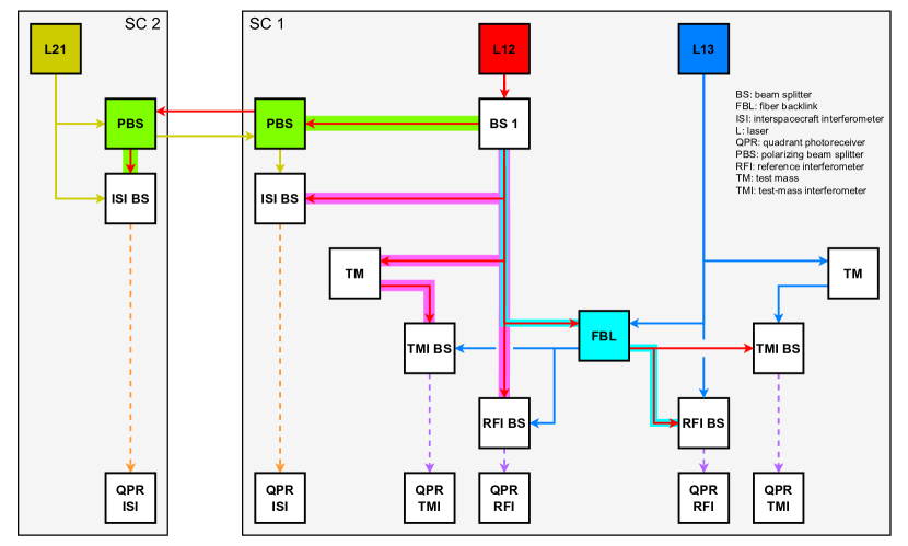
Figure 1: We trace laser 12 (red arrows) to the local and to the distant ISI, where it interferes with the distant laser 21 (yellow arrows) to form beat notes (orange dashed arrows). We further trace laser 12 to the local TMI and RFI and to the adjacent TMI and RFI, where it interferes with the adjacent laser 13 (blue arrows) to form beat notes (purple dashed arrows). The reference point is the BS dividing outgoing and local beams (BS 1 according to the notation in [12]). The OOPLs from BS 1 to the recombining BSs at the local, adjacent, and distant interferometers are highlighted pink, light blue, and green, respectively.

Apart from interspacecraft signal propagation delays, also delays due to onboard signal propagation and processing emerge in the TDI combinations. However, these onboard delays were mostly neglected or only partially considered in previous TDI-related research. Onboard delays can be grouped into two categories: (1) Onboard delays that occur after the recombining beam splitters (BSs) at the different interferometers are common to both interfering beams, e.g., electronic delays in the QPRs and signal processing delays in the phasemeter. A detailed investigation of common onboard delays can be found in [13]. (2) Onboard delays before the recombining BSs differ between both interfering beams. These are onboard optical path lengths (OOPLs) between the laser sources and the recombining BSs (see fig. 1). [14] studied OOPLs in the ISI but neglected TMI and RFI. However, also OOPLs in TMI and RFI cause residual laser noise in the TDI combinations if uncompensated. While previous research established models for the coupling of ISI OOPLs in TDI, where they act as ranging biases [15, 16], we lack such models for the coupling of TMI and RFI OOPLs.

This paper studies the TDI coupling of OOPLs in all interferometers. In section II, we introduce delay and advancement operators for OOPLs. This allows us to express the LISA beat notes, including OOPLs. In section III, we derive a compensation scheme for OOPLs, which includes the OOPL delay and advancement operators in the TDI processing steps. We numerically implement this OOPL compensation scheme and demonstrate its performance in section V. In section IV, we derive analytical models for the coupling of OOPLs in TDI and compare these models with our numerical results in section V. We conclude in section VI.

II LISA beat notes with onboard optical path lengths

II.1 Brief summary of the LISA payload

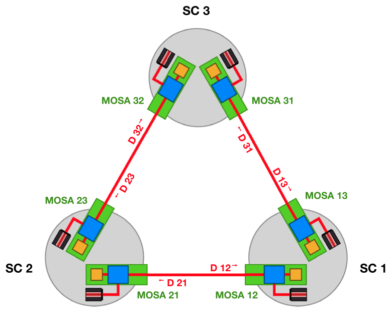
Figure 2: LISA labeling conventions (from [17]). The SC are labeled clockwise. The MOSAs and associated building blocks (lasers, interferometers, etc.) are labeled with 2 indices: The first one denotes the SC they are located on, the second one the SC they are facing. Left-handed MOSAs are labeled 12, 23, 31. Right-handed MOSAs are labeled 13, 32, 21.

Each SC contains two movable optical subassemblies (MOSAs), which are oriented toward the other two SC of the constellation (the labeling conventions are summarized in fig. 2). Each MOSA has a laser, which is fiber-fed to an optical bench (OB) made of Zerodur. From there, the laser is transmitted to the distant SC via a telescope and to the adjacent MOSA via an optical fiber (the backlink). On the OB itself, the laser serves as a local oscillator in three heterodyne interferometers: The interspacecraft interferometer (ISI) interferes the local beam with the beam received from the distant SC; the test-mass interferometer (TMI) and the reference interferometer (RFI) interfere the local beam with the beam received from the adjacent MOSA. Before interference in the TMI, the local beam is reflected off a free-falling cubic gold-platinum test mass along the intersatellite axis.

II.2 Delay operators

We neglect clock effects and express all quantities in terms of a virtual LISA constellation time $\tau$. Following the notation of [18], we write the frequency of laser $ij$ in terms of its offset $O_{ij}$ from the nominal laser frequency $\nu_{0}$ and laser frequency noise $\dot{p}_{ij}$:

$$\nu_{ij}(\tau)=\nu_{0}+O_{ij}(\tau)+\dot{p}_{ij}(\tau).$$ (1)

This frequency is defined at the laser source. To model the LISA beat notes, we must compare the beam frequencies at the recombining beam splitters (BSs) of the different interferometers. This requires the concept of delay operators.

The interspacecraft delay operator $\textbf{D}_{ij}$ delays the time argument of the beam phase $\Phi_{ji}$ by the intersatellite signal propagation time to SC $i$ from SC $j$, denoted $d_{ij}$:

$$\textbf{D}_{ij}\>\Phi_{ji}(\tau) =\Phi_{ji}\left(\tau-d_{ij}(\tau)\right).$$ (2)

Here, we express the LISA beat notes in frequency, i.e., we must take the time derivative of eq. 2:

$$\dot{\textbf{D}}_{ij}\>\nu_{ji}(\tau)\vcentcolon=\left(1-\dot{d}_{ij}(\tau)\right)\>\nu_{ji}\left(\tau-d_{ij}(\tau)\right),$$ (3)

where $\dot{\textbf{D}}_{ij}$ denotes the Doppler-delay operator [17].

In addition to interspacecraft signal propagation delays, we must consider delays due to onboard signal propagation and processing. We briefly revisit our categorization of onboard delays from section I: (1) Onboard delays occurring after the recombining BSs are common to both interfering beams. We here neglect common onboard delays. They can be compensated by time-shifting the beatnotes in an initial data treatment [13]. (2) Onboard delays occurring before the recombining BSs differ between both interfering beams. These are delays due to onboard optical path lengths (OOPLs) between the laser sources and the recombining BSs (see fig. 1). They are the subject of this paper. Below, we neglect the conversion between optical path lengths and the associated optical delays and use these terms interchangeable.

To express the LISA beat notes, including OOPLs, we introduce the onboard delay operator for OOPLs:

$$\dot{\textbf{D}}_{\text{ifo}}^{\text{beam}}\>\nu_{ij}(\tau) =\left(1-\dot{d}_{\text{ifo}}^{\text{beam}}\right)\nu_{ij}\left(\tau-d_{\text{ifo}}^{\text{beam}}\right)$$

$$\approx\nu_{ij}\left(\tau-d_{\text{ifo}}^{\text{beam}}\right)=\vcentcolon\textbf{D}_{\text{ifo}}^{\text{beam}}\>\nu_{ij}(\tau).$$ (4)

ifo is a placeholder for the target interferometer. Thus, it takes on the symbols isi, tmi, and rfi. beam is a placeholder for the particular beam. It distinguishes between local, adjacent, and distant beams denoted by loc, adj, and dist. We consider OOPLs constant at the scales applicable for laser noise suppression and neglect the associated Doppler terms.

For a constant delay operator $\textbf{D}_{x}$ we define the associated advancement operator $\textbf{A}_{x}$, which acts as its inverse:

$$\textbf{A}_{x}\>\nu_{ij}(\tau)\vcentcolon= \>\nu_{ij}\left(\tau+x\right),$$ (5)

$$\textbf{A}_{x}\>\textbf{D}_{x}\>\nu_{ij}(\tau)= \>\nu_{ij}\left(\tau-x+x\right)=\nu_{ij}(\tau),$$ (6)

where $x$ is a placeholder for the concrete delay.

II.3 LISA beat notes with onboard optical delays

Each laser enters six interferometers: the ISI, TMI, and RFI on the local MOSA, the TMI and RFI on the adjacent MOSA, and the ISI on the distant MOSA. The OOPL delay operator (see section II.2) allows us to write the LISA beat notes including the OOPLs between the laser sources and the recombining BSs at these interferometers (see fig. 1):

$$\text{isi}_{ij} =\textbf{D}_{\text{isi}}^{\text{rec}}\>\dot{\textbf{D}}_{ij}\>\textbf{D}_{\text{isi}}^{\text{out}}\>\nu_{ji}-\textbf{D}_{\text{isi}}^{\text{loc}}\>\nu_{ij}+\dot{N}_{ij}^{\text{isi}},$$ (7)

$$\text{tmi}_{ij} =\textbf{D}_{\text{tmi}}^{\text{adj}}\>\nu_{ik}-\textbf{D}_{\text{tmi}}^{\text{loc}}\>\nu_{ij}+\dot{N}_{ij}^{\text{tmi}},$$ (8)

$$\text{rfi}_{ij} =\textbf{D}_{\text{rfi}}^{\text{adj}}\>\nu_{ik}-\textbf{D}_{\text{rfi}}^{\text{loc}}\>\nu_{ij}+\dot{N}_{ij}^{\text{rfi}},$$ (9)

$\textbf{D}_{\text{isi}}^{\text{out}}$ and $\textbf{D}_{\text{isi}}^{\text{rec}}$ denote the OOPLs of the distant beam on the distant and local SC, respectively. Laser frequency noise $\dot{p}_{ij}$ is included in the laser frequency (see eq. 1). All other noises are summarized in $\dot{N}^{\text{ifo}}_{ij}$.

Like the individual laser frequencies, the LISA beat notes can be decomposed into large offsets and small fluctuations. We want to study laser frequency noise cancellation in the presence of OOPLs, so we focus on the latter and write eqs. 7, 8 and 9 as

$$\text{isi}_{ij} =\textbf{D}_{\text{isi}}^{\text{rec}}\>\dot{\textbf{D}}_{ij}\>\textbf{D}_{\text{isi}}^{\text{out}}\>\dot{p}_{ji}-\textbf{D}_{\text{isi}}^{\text{loc}}\>\dot{p}_{ij},$$ (10)

$$\text{tmi}_{ij} =\textbf{D}_{\text{tmi}}^{\text{adj}}\>\dot{p}_{ik}-\textbf{D}_{\text{tmi}}^{\text{loc}}\>\dot{p}_{ij},$$ (11)

$$\text{rfi}_{ij} =\textbf{D}_{\text{rfi}}^{\text{adj}}\>\dot{p}_{ik}-\textbf{D}_{\text{rfi}}^{\text{loc}}\>\dot{p}_{ij},$$ (12)

where we dropped the noise terms $\dot{N}^{\text{ifo}}_{ij}$ for the ease of notation. We can commute $\dot{\textbf{D}}_{ij}$ and $\textbf{D}_{\text{isi}}^{\text{rec}}$, since

$$\>\textbf{D}_{\text{isi}}^{\text{rec}}\>\dot{\textbf{D}}_{ij}\>\dot{p}(\tau)$$

$$= \>\left(1-\dot{d}_{ij}(\tau-d_{\text{isi}}^{\text{rec}})\right)\dot{p}\left(\tau-d_{\text{isi}}^{\text{rec}}-d_{ij}\left(\tau-d_{\text{isi}}^{\text{rec}}\right)\right)$$

$$\approx \>\left(1-\dot{d}_{ij}+\ddot{d}_{ij}\cdot d_{\text{isi}}^{\text{rec}}\right)\dot{p}\left(\tau-d_{\text{isi}}^{\text{rec}}-d_{ij}+\dot{d}_{ij}\cdot d_{\text{isi}}^{\text{rec}}\right)$$

$$\approx \>\left(1-\dot{d}_{ij}(\tau)\right)\dot{p}\left(\tau-d_{\text{isi}}^{\text{rec}}-d_{ij}(\tau)\right)$$

$$= \>\dot{\textbf{D}}_{ij}\>\textbf{D}_{\text{isi}}^{\text{rec}}\>\dot{p}(\tau),$$ (13)

where we applied the following approximations (considering ESA orbits [19]):

$$c\cdot\dot{d}_{ij}\cdot d_{\text{isi}}^{\text{rec}} \lessapprox$10\text{\,}\mathrm{m}\text{\,}{\mathrm{s}}^{-1}$\cdot$10\text{\,}\mathrm{ns}$=$0.1\text{\,}\mathrm{\SIUnitSymbolMicro m}$,$$ (14)

$$c\cdot\ddot{d}_{ij}\cdot d_{\text{isi}}^{\text{rec}} \lessapprox$10\text{\,}\mathrm{\SIUnitSymbolMicro m}\text{\,}{\mathrm{s}}^{-2}$\cdot$10\text{\,}\mathrm{ns}$=$0.1\text{\,}\mathrm{pm}\text{\,}{\mathrm{s}}^{-1}$.$$ (15)

These terms are negligible considering the achievable accuracy for intersatelite ranging. Hence, we can write

$$\text{isi}_{ij}= \>\dot{\textbf{D}}_{ij}\>\textbf{D}_{\text{isi}}^{\text{dist}}\>\dot{p}_{ji}-\textbf{D}_{\text{isi}}^{\text{loc}}\>\dot{p}_{ij},$$ (16)

$$\textbf{D}_{\text{isi}}^{\text{dist}}\vcentcolon= \>\textbf{D}_{\text{isi}}^{\text{rec}}\>\textbf{D}_{\text{isi}}^{\text{out}}.$$ (17)

In summary, we need to consider six OOPLs: $\textbf{D}_{\text{isi}}^{\text{loc}}$, $\textbf{D}_{\text{isi}}^{\text{dist}}$, $\textbf{D}_{\text{tmi}}^{\text{loc}}$, $\textbf{D}_{\text{tmi}}^{\text{adj}}$, $\textbf{D}_{\text{rfi}}^{\text{loc}}$, and $\textbf{D}_{\text{rfi}}^{\text{adj}}$. Their current design values can be estimated from [12]; we list them in the first column of table 1. We expect manufacturing asymmetries in the order of $10100\text{\,}\mathrm{\SIUnitSymbolMicro m}$. We assess their impact in appendix A. We neglect manufacturing asymmetries in the notation, i.e., we do not specify MOSA indices for OOPL delay and advancement operators.

	Current OB Design	Matched OB Design
$d_{\text{isi}}^{\text{loc}}$	$0.31\text{\,}\mathrm{m}$	$0.31\text{\,}\mathrm{m}$
$d_{\text{isi}}^{\text{dist}}$	$0.59\text{\,}\mathrm{m}$	$0.59\text{\,}\mathrm{m}$
$d_{\text{tmi}}^{\text{loc}}$	$0.41\text{\,}\mathrm{m}$	$0.41\text{\,}\mathrm{m}$
$d_{\text{tmi}}^{\text{adj}}$	$10.71\text{\,}\mathrm{m}$	$10.71\text{\,}\mathrm{m}$
$d_{\text{rfi}}^{\text{loc}}$	$0.36\text{\,}\mathrm{m}$	$0.36\text{\,}\mathrm{m}$
$d_{\text{rfi}}^{\text{adj}}$	$10.64\text{\,}\mathrm{m}$	$10.66\text{\,}\mathrm{m}$

Table 1: First column: OOPLs as estimated from [12] under the assumption of a $10\text{\,}\mathrm{m}$ fiber length. Second column: a set of OOPLs fulfilling the OB design guideline eq. 28.

III Time-delay interferometry with onboard optical delays

III.1 Brief review of time-delay interferometry

Time-delay interferometry (TDI) is an on-ground data processing technique for LISA. It time shifts and linearly combines the various interferometric measurements to construct virtual equal-optical-path-length interferometers between the six free-falling test masses. Thus, it mitigates laser frequency noise and optical bench jitter. TDI can be divided into three steps [11]:

(1) ISI, TMI, and RFI beat notes are combined to set up measurements for the interspacecraft-test-mass-to-test-mass separations according to the split interferometry concept. These measurements are called the intermediary TDI $\xi$ variables and are given by

$$\xi_{ij}=\text{isi}_{ij}+\frac{\text{rfi}_{ij}-\text{tmi}_{ij}}{2}+\dot{\textbf{D}}_{ij}\frac{\text{rfi}_{ji}-\text{tmi}_{ji}}{2}.$$ (18)

The ISI measures distance variations between local and distant OBs. The differences between RFI and TMI beat notes constitute measurements of the OB versus test mass motion on the local and distant SC, respectively.

(2) The RFI beat notes are applied to remove three of six laser noise sources from the intermediary $\xi$ variables. We take the differences between both RFI beat notes on the same SC to cancel the reciprocal part of the fiber backlink noise. These differences are combined with the intermediary $\xi$ variables (see eq. 18) to form the intermediary TDI $\eta$ variables, where laser noise contributions of right-handed lasers (those associated with the MOSAs 13, 32, and 21) cancel:

$$\eta_{13} =\xi_{13}+\frac{\text{rfi}_{12}-\text{rfi}_{13}}{2},$$ (19)

$$\eta_{12} =\xi_{12}+\dot{\textbf{D}}_{12}\>\frac{\text{rfi}_{21}-\text{rfi}_{23}}{2}.$$ (20)

The remaining $\eta$ variables result from cyclic permutation of the SC indices.

(3) The $\eta$ variables are combined to form virtual equal-optical-path-length interferometers, in which laser frequency noise naturally cancels. For example, the second-generation TDI Michelson variable $X_{2}$ denotes [17]

$$X_{2}=\left(1-\dot{\textbf{D}}_{121}-\dot{\textbf{D}}_{12131}+\dot{\textbf{D}}_{1312121}\right)\left(\eta_{13}+\dot{\textbf{D}}_{13}\>\eta_{31}\right)$$

$$-\left(1-\dot{\textbf{D}}_{131}-\dot{\textbf{D}}_{13121}+\dot{\textbf{D}}_{1213131}\right)\left(\eta_{12}+\dot{\textbf{D}}_{12}\>\eta_{21}\right),$$ (21)

$Y_{2}$ and $Z_{2}$ can be obtained via cyclic permutation of the SC indices.

Previous research neglected the coupling of OOPLs in these three steps. Without proper treatment, they cause laser noise residuals. We present analytical models for these residuals in section IV. In this section, we derive a compensation scheme for OOPLs in TDI: We compensate for the corresponding delays by including OOPL delay and advancement operators in the three TDI steps. Below, we refer to the thus updated TDI algorithm as the OOPL compensation scheme (OOPL-CS).

III.2 Removal of optical bench jitter with OOPLs

Without compensation, mismatches in the OOPLs between TMI and RFI cause laser noise residuals in the intermediary TDI $\xi$ variables. To compensate for this, we include OOPL delay/advancement operators $\textbf{D}_{\text{a}}$ and $\textbf{D}_{\text{b}}$ in the $\xi$ variables:

$$\xi_{ij}=\text{isi}_{ij}+\frac{\textbf{D}_{\text{a}}\text{rfi}_{ij}-\textbf{D}_{\text{b}}\text{tmi}_{ij}}{2}+\dot{\textbf{D}}_{ij}\frac{\textbf{D}_{\text{a}}\text{rfi}_{ji}-\textbf{D}_{\text{b}}\text{tmi}_{ji}}{2}.$$ (22)

To derive the required operators $\textbf{D}_{\text{a}}$ and $\textbf{D}_{\text{b}}$ we expand the laser noise terms in the numerators of eq. 22:

$$\>\textbf{D}_{\text{a}}\>\text{rfi}_{ij}-\textbf{D}_{\text{b}}\>\text{tmi}_{ij}$$ (23)

$$= \left(\textbf{D}_{\text{a}}\textbf{D}_{\text{rfi}}^{\text{adj}}-\textbf{D}_{\text{b}}\textbf{D}_{\text{tmi}}^{\text{adj}}\right)\dot{p}_{ik}-\left(\textbf{D}_{\text{a}}\textbf{D}_{\text{rfi}}^{\text{loc}}-\textbf{D}_{\text{b}}\textbf{D}_{\text{tmi}}^{\text{loc}}\right)\dot{p}_{ij}$$

$$= \>\dot{p}_{ik}(\tau-d_{\text{a}}-d_{\text{rfi}}^{\text{adj}})-\dot{p}_{ik}(\tau-d_{\text{b}}-d_{\text{tmi}}^{\text{adj}})$$

$$- \>\dot{p}_{ij}(\tau-d_{\text{a}}-d_{\text{rfi}}^{\text{loc}})+\dot{p}_{ij}(\tau-d_{\text{b}}-\>d_{\text{tmi}}^{\text{loc}})$$ (24)

$$\approx \left(d_{\text{a}}-d_{\text{b}}+d_{\text{rfi}}^{\text{loc}}-d_{\text{tmi}}^{\text{loc}}\right)\ddot{p}_{ij}$$

$$- \>(d_{\text{a}}-d_{\text{b}}+d_{\text{rfi}}^{\text{adj}}-d_{\text{tmi}}^{\text{adj}})\>\ddot{p}_{ik}.$$ (25)

We do not consider the contribution of the the $\dddot{p}$ terms: The two extra time derivatives with respect to $\dot{p}$ give a factor of $(2\pi f)^{2}$ in terms of amplitude spectral density (ASD); the OOPLs can be approximated with $10\text{\,}\mathrm{ns}$; consequently, the laser noise contribution of the $\dddot{p}$ terms is suppressed by a factor of $10^{-16}${\mathrm{s}}^{2}$\times(2\pi f)^{2}$, which is completely negligible across the LISA band.

The $\ddot{p}$ terms cannot be dropped so easily. We need to choose the operators $\textbf{D}_{\text{a}}$ and $\textbf{D}_{\text{b}}$ such that the $\ddot{p}$ terms in eq. 25 cancel. This yields two conditions:

$$d_{a}-d_{b} =d_{\text{tmi}}^{\text{loc}}-d_{\text{rfi}}^{\text{loc}},$$ (26)

$$d_{a}-d_{b} =d_{\text{tmi}}^{\text{adj}}-d_{\text{rfi}}^{\text{adj}}.$$ (27)

They can be combined to form a guideline for the optical bench design:

$$d_{\text{rfi}}^{\text{loc}}-d_{\text{tmi}}^{\text{loc}}=d_{\text{rfi}}^{\text{adj}}-d_{\text{tmi}}^{\text{adj}},$$ (28)

i.e., the difference between the local OOPLs in TMI and RFI has to match the difference between the adjacent OOPLs in these interferometers. This should not be understood as a strict requirement but rather as a design guideline. In fact, the current design values (see the first column in table 1) involve a mismatch of about $2\text{\,}\mathrm{cm}$. We assess the impact of this mismatch analytically in section IV and numerically in section V.

If the OB design guideline is fulfilled exactly, we can cancel the $\ddot{p}$ laser noise terms entirely by choosing the delay operators $\textbf{D}_{\text{a}}$ and $\textbf{D}_{\text{b}}$ according to

$$\textbf{D}_{\text{a}}\>\textbf{D}_{\text{b}} =\textbf{D}_{\text{tmi}}^{\text{loc}}\>\textbf{A}_{\text{rfi}}^{\text{loc}},$$ (29)

which is fulfilled by, e.g.,

$$\textbf{D}_{\text{a}} =\textbf{D}_{\text{tmi}}^{\text{loc}}\>\textbf{A}_{\text{rfi}}^{\text{loc}},$$ (30)

$$\textbf{D}_{\text{b}} =\textbf{D}_{\text{id}}.$$ (31)

$\textbf{D}_{\text{id}}$ denotes the identity element, which does not change the time argument of the function it is acting on. Thus, we can cancel laser noise terms in the difference between RFI and TMI up to and including the $\ddot{p}$ terms. The intermediary TDI variables $\xi$ can now be written as

$$\xi_{ij}=\text{isi}_{ij}+\dot{N}^{\xi}_{ij},$$ (32)

where $\dot{N}^{\xi}_{ij}$ summarizes backlink, test-mass-acceleration, and readout noise of all constituent beat notes.

III.3 Reduction to three lasers with OOPLs

Due to the fiber backlink, local and adjacent OOPLs in the RFI differ by about $10\text{\,}\mathrm{m}$ (see table 1). If uncompensated, this causes residual laser noise in the intermediary TDI $\eta$ variables. Similarly, OOPL mismatches between ISI and RFI lead to residual laser noise. To compensate for this, we include OOPL delay/advancement operators $\textbf{D}_{\text{c}}$, $\textbf{D}_{\text{d}}$, $\textbf{D}_{\text{e}}$, and $\textbf{D}_{\text{f}}$ in the $\eta$ variables:

$$\eta_{13} =\xi_{13}+\textbf{D}_{\text{e}}\>\frac{\textbf{D}_{\text{c}}\>\text{rfi}_{12}-\textbf{D}_{\text{d}}\>\text{rfi}_{13}}{2},$$ (33)

$$\eta_{12} =\xi_{12}+\dot{\textbf{D}}_{12}\>\textbf{D}_{\text{f}}\>\frac{\textbf{D}_{\text{d}}\>\text{rfi}_{21}-\textbf{D}_{\text{c}}\>\text{rfi}_{23}}{2}.$$ (34)

We apply $\textbf{D}_{\text{c}}$ to the left-handed RFI beat notes and $\textbf{D}_{\text{d}}$ to the right-handed ones. $\textbf{D}_{\text{e}}$ and $\textbf{D}_{\text{f}}$ are applied to match the OOPLs between the ISIs and RFIs.

To derive the operators $\textbf{D}_{\text{c}}$ and $\textbf{D}_{\text{d}}$ we expand the numerator of eq. 33 up to the first order, i.e., up to $\ddot{p}$:

$$\>\textbf{D}_{\text{c}}\>\text{rfi}_{12}-\textbf{D}_{\text{d}}\>\text{rfi}_{13}$$ (35)

$$= \left(\textbf{D}_{\text{c}}\textbf{D}_{\text{rfi}}^{\text{adj}}+\textbf{D}_{\text{d}}\textbf{D}_{\text{rfi}}^{\text{loc}}\right)\dot{p}_{13}-\left(\textbf{D}_{\text{c}}\textbf{D}_{\text{rfi}}^{\text{loc}}+\textbf{D}_{\text{d}}\textbf{D}_{\text{rfi}}^{\text{adj}}\right)\dot{p}_{12}$$

$$= \>\dot{p}_{13}(\tau-d_{\text{c}}-d_{\text{rfi}}^{\text{adj}})+\dot{p}_{13}(\tau-d_{\text{d}}-d_{\text{rfi}}^{\text{loc}})$$

$$- \>\dot{p}_{12}(\tau-d_{\text{c}}-d_{\text{rfi}}^{\text{loc}})-\dot{p}_{12}(\tau-d_{\text{d}}-d_{\text{rfi}}^{\text{adj}})$$ (36)

$$\approx \>2\>\dot{p}_{13}-\ddot{p}_{13}\cdot\left(d_{\text{c}}+d_{\text{d}}+d_{\text{rfi}}^{\text{loc}}+d_{\text{rfi}}^{\text{adj}}\right)$$

$$- \>2\>\dot{p}_{12}+\ddot{p}_{12}\cdot\left(d_{\text{c}}+d_{\text{d}}+d_{\text{rfi}}^{\text{loc}}+d_{\text{rfi}}^{\text{adj}}\right).$$ (37)

The $\dddot{p}$ can be neglected as explained in section III.2. We want to choose the operators $\textbf{D}_{\text{c}}$ and $\textbf{D}_{\text{d}}$ such that the $\ddot{p}$ terms in this expansion cancel. The computation above yields one condition:

$$d_{\text{c}}+d_{\text{d}}+d_{\text{rfi}}^{\text{loc}}+d_{\text{rfi}}^{\text{adj}}=0,$$ (38)

or in terms of operators

$$\textbf{D}_{\text{c}}\>\textbf{D}_{\text{d}}\>\textbf{D}_{\text{rfi}}^{\text{loc}}\>\textbf{D}_{\text{rfi}}^{\text{adj}}=\textbf{D}_{\text{id}},$$ (39)

where the operators commute as the delays are constant. One solution to eq. 39 is given by

$$\textbf{D}_{\text{c}} =\textbf{A}_{\text{rfi}}^{\text{loc}},$$ (40)

$$\textbf{D}_{\text{d}} =\textbf{A}_{\text{rfi}}^{\text{adj}}.$$ (41)

We then obtain

$$\>\textbf{A}_{\text{rfi}}^{\text{loc}}\text{rfi}_{12}-\textbf{A}_{\text{rfi}}^{\text{adj}}\text{rfi}_{13}$$ (42)

$$= \>-2\>\dot{p}_{12}-\left(\textbf{A}_{\text{rfi}}^{\text{loc}}\>\textbf{D}_{\text{rfi}}^{\text{adj}}+\textbf{A}_{\text{rfi}}^{\text{adj}}\>\textbf{D}_{\text{rfi}}^{\text{loc}}\right)\dot{p}_{13}$$ (43)

$$\approx \>2\>\dot{p}_{13}-2\>\dot{p}_{12},$$ (44)

to first order. The same result can be derived by considering the numerator of eq. 34.

Now we derive the operators $\textbf{D}_{\text{e}}$ and $\textbf{D}_{\text{f}}$ to match the OOPLs between ISI and RFI. Choosing $\textbf{D}_{\text{c}}$ and $\textbf{D}_{\text{d}}$ according to eqs. 40 and 41 allows us to write the right-handed $\eta$ variable as:

$$\eta_{13}= \>\text{isi}_{13}+\textbf{D}_{\text{e}}\left(\dot{p}_{13}-\>\dot{p}_{12}\right)$$ (45)

$$= \>\dot{\textbf{D}}_{13}\>\textbf{D}_{\text{isi}}^{\text{dist}}\>\dot{p}_{31}-\textbf{D}_{\text{e}}\>\dot{p}_{12}$$

$$- \>\textbf{D}_{\text{isi}}^{\text{loc}}\>\dot{p}_{13}+\textbf{D}_{\text{e}}\>\dot{p}_{13}.$$ (46)

To cancel the laser frequency noise of the right-handed laser $13$, we set

$$\textbf{D}_{\text{e}}=\textbf{D}_{\text{isi}}^{\text{loc}},$$ (47)

so that the right-handed $\eta$ variable becomes

$$\eta_{13}=\dot{\textbf{D}}_{13}\>\textbf{D}_{\text{isi}}^{\text{dist}}\>\dot{p}_{31}-\textbf{D}_{\text{isi}}^{\text{loc}}\>\dot{p}_{12}.$$ (48)

With eqs. 40 and 41 the left-handed intermediary $\eta$ variable can be written as

$$\eta_{12}= \>\text{isi}_{12}+\dot{\textbf{D}}_{12}\>\textbf{D}_{\text{f}}\>\left(\dot{p}_{23}-\dot{p}_{21}\right)$$ (49)

$$= \>\dot{\textbf{D}}_{12}\>\textbf{D}_{\text{f}}\>\dot{p}_{23}-\textbf{D}_{\text{isi}}^{\text{loc}}\>\dot{p}_{12}$$

$$+ \>\dot{\textbf{D}}_{12}\>\textbf{D}_{\text{isi}}^{\text{dist}}\>\dot{p}_{21}-\dot{\textbf{D}}_{12}\>\textbf{D}_{\text{f}}\>\dot{p}_{21}.$$ (50)

We want to cancel the right-handed laser 21, so we set

$$\textbf{D}_{\text{f}}=\textbf{D}_{\text{isi}}^{\text{dist}},$$ (51)

and the left-handed $\eta$ variable becomes

$$\eta_{12} =\dot{\textbf{D}}_{12}\>\textbf{D}_{\text{isi}}^{\text{dist}}\>\dot{p}_{23}-\textbf{D}_{\text{isi}}^{\text{loc}}\>\dot{p}_{12}.$$ (52)

Thus, we cancel the laser frequency noise contributions of right-handed lasers (up to and including second order $\ddot{p}$) by including the OOPL delay/advancement operators $\textbf{D}_{\text{c}}$, $\textbf{D}_{\text{d}}$, $\textbf{D}_{\text{e}}$, and $\textbf{D}_{\text{f}}$ as defined in eqs. 40, 41, 47 and 51 in the $\eta$ variables eqs. 33 and 34.

III.4 Laser-noise-free TDI combinations with OOPLs

Laser-noise-free TDI combinations like the second-generation TDI Michelson variable $X_{2}$ (see section III.1) are linear combinations of the $\eta$ variables delayed by interspacecraft delay operators $\dot{\textbf{D}}_{ij}$. While $\dot{\textbf{D}}_{ij}$ just accounts for the interspacecraft signal propagation time (defined between the PBSs on receiving and emitting SC), the $\eta$ variables are defined at the recombining BS of the ISI (we neglect subsequent common delays due to analog and digital signal processing). Hence, the OOPLs in the ISI cause residual laser frequency noise if uncompensated.

[14] considers a TDI toy model to derive an operator $\dot{\mathcal{D}}_{ij}$ that accounts for onboard delays. This TDI delay operator then replaces $\dot{\textbf{D}}_{ij}$ in the TDI combinations. However, the TDI steps 1 and 2 are neglected there, and the TDI delay operator is directly computed from the ISI beat notes. We, therefore, revisit that toy model here and rebuild it upon the intermediary TDI $\eta$ variables as derived in section III.3.

We combine $\eta_{12}$ and $\eta_{21}$ and focus on canceling the noise of laser $12$:

$$\dot{\mathcal{D}}_{21}\>\eta_{12}+\eta_{21}= \>\dot{\mathcal{D}}_{21}\left(\dot{\textbf{D}}_{12}\>\textbf{D}_{\text{isi}}^{\text{dist}}\>\dot{p}_{23}-\textbf{D}_{\text{isi}}^{\text{loc}}\>\dot{p}_{12}\right)$$

$$+ \>\dot{\textbf{D}}_{21}\>\textbf{D}_{\text{isi}}^{\text{dist}}\>\dot{p}_{12}-\textbf{D}_{\text{isi}}^{\text{loc}}\>\dot{p}_{23},$$ (53)

$$=\>\Big{(}\dot{\textbf{D}}_{21}\>\textbf{D}_{\text{isi}}^{\text{dist}}-\dot{\mathcal{D}}_{21} \>\textbf{D}_{\text{isi}}^{\text{loc}}\Big{)}\dot{p}_{12}+(...)\>\dot{p}_{23}.$$ (54)

To cancel $\dot{p}_{12}$, we need to choose $\dot{\mathcal{D}}_{21}$ such that the first bracket vanishes, i.e.,

$$\dot{\textbf{D}}_{21}\>\textbf{D}_{\text{isi}}^{\text{dist}}=\dot{\mathcal{D}}_{21} \>\textbf{D}_{\text{isi}}^{\text{loc}}.$$ (55)

Multiplying this expression with $\textbf{A}_{\text{isi}}^{\text{loc}}$ from the right yields the TDI delay operator

$$\dot{\mathcal{D}}_{21}=\dot{\textbf{D}}_{21}\>\textbf{D}_{\text{isi}}^{\text{dist}}\>\textbf{A}_{\text{isi}}^{\text{loc}},$$ (56)

which accounts for OOPLs in the ISI. It replaces $\dot{\textbf{D}}$ in the laser-noise-free TDI combinations, e.g., section III.1 becomes

$$X_{2}=\left(1-\dot{\mathcal{D}}_{121}-\dot{\mathcal{D}}_{12131}+\dot{\mathcal{D}}_{1312121}\right)\left(\eta_{13}+\dot{\mathcal{D}}_{13}\>\eta_{31}\right)$$

$$-\left(1-\dot{\mathcal{D}}_{131}-\dot{\mathcal{D}}_{13121}+\dot{\mathcal{D}}_{1213131}\right)\left(\eta_{12}+\dot{\mathcal{D}}_{12}\>\eta_{21}\right).$$ (57)

Other TDI combinations can be updated analogously by replacing the $\dot{\textbf{D}}$ operators with $\dot{\mathcal{D}}$ operators.

IV Impact of onboard optical Delays

In the previous section, we derived an OOPL compensation scheme for TDI, which includes OOPL delay and advancement operators in the TDI equations. In this section, we derive analytical models for the coupling of OOPLs in TDI if uncompensated. We focus on the first two steps (computation of the intermediary TDI variables $\xi$ and $\eta$). In the third TDI step, OOPLs act as biases; their effect has been studied in [15, 16].

We start with the intermediary TDI $\xi$ variables (see eq. 18). Now we do not compensate OOPLs with the operators $\textbf{D}_{\text{a}}$ and $\textbf{D}_{\text{b}}$ as in eq. 22. Expanding the difference between RFI and TMI beat notes to first order gives:

$$\text{rfi}_{ij}-\text{tmi}_{ij}= \>\dot{p}_{ik}(\tau-d_{\text{rfi}}^{\text{adj}})-\dot{p}_{ij}(\tau-d_{\text{rfi}}^{\text{loc}})$$

$$- \left(\dot{p}_{ik}(\tau-d_{\text{tmi}}^{\text{adj}})-\dot{p}_{ij}(\tau-d_{\text{tmi}}^{\text{loc}})\right)$$ (58)

$$\approx \>\dot{p}_{ik}-d_{\text{rfi}}^{\text{adj}}\>\ddot{p}_{ik}-\dot{p}_{ij}+d_{\text{rfi}}^{\text{loc}}\>\ddot{p}_{ij}$$

$$- \>\dot{p}_{ik}+d_{\text{tmi}}^{\text{adj}}\>\ddot{p}_{ik}+\dot{p}_{ij}-d_{\text{tmi}}^{\text{loc}}\>\ddot{p}_{ij}$$ (59)

$$= \>d_{\Delta}^{\text{loc}}\>\ddot{p}_{ij}-d_{\Delta}^{\text{adj}}\>\ddot{p}_{ik},$$ (60)

where we introduce the abbreviations

$$d_{\Delta}^{\text{loc}} =d_{\text{rfi}}^{\text{loc}}-d_{\text{tmi}}^{\text{loc}},$$ (61)

$$d_{\Delta}^{\text{adj}} =d_{\text{rfi}}^{\text{adj}}-d_{\text{tmi}}^{\text{adj}}$$ (62)

for mismatches between OOPLs in TMI and RFI. Inserting eq. 60 into the $\xi$ variables yields:

$$\xi_{ij}= \>\text{isi}_{ij}+\frac{d_{\Delta}^{\text{loc}}\ddot{p}_{ij}-d_{\Delta}^{\text{adj}}\ddot{p}_{ik}}{2}+\dot{\textbf{D}}_{ij}\frac{d_{\Delta}^{\text{loc}}\ddot{p}_{ji}-d_{\Delta}^{\text{adj}}\ddot{p}_{jk}}{2}$$ (63)

$$= \>\text{isi}_{ij}+C^{\xi}_{ij},$$ (64)

$$C^{\xi}_{ij}\vcentcolon= \>\frac{d_{\Delta}^{\text{loc}}\>\ddot{p}_{ij}-d_{\Delta}^{\text{adj}}\>\ddot{p}_{ik}}{2}+\dot{\textbf{D}}_{ij}\frac{d_{\Delta}^{\text{loc}}\>\ddot{p}_{ji}-d_{\Delta}^{\text{adj}}\>\ddot{p}_{jk}}{2},$$ (65)

where $C^{\xi}_{ij}$ is the correction term due to OOPLs.

We proceed with the intermediary TDI $\eta$ variables (see eqs. 19 and 20). Now we do not compensate OOPLs with the operators $\textbf{D}_{\text{c}}$ to $\textbf{D}_{\text{f}}$ as in eqs. 33 and 34. We expand the ISI and RFI beat notes to first order:

$$\text{rfi}_{ij} \approx\dot{p}_{ik}-d_{\text{rfi}}^{\text{adj}}\>\ddot{p}_{ik}-\left(\dot{p}_{ij}-d_{\text{rfi}}^{\text{loc}}\>\ddot{p}_{ij}\right),$$ (66)

$$\text{isi}_{ij} \approx\dot{\textbf{D}}_{ij}\left(\dot{p}_{ji}-d_{\text{isi}}^{\text{dist}}\>\ddot{p}_{ji}\right)-\left(\dot{p}_{ij}-d_{\text{isi}}^{\text{loc}}\>\ddot{p}_{ij}\right).$$ (67)

Inserting eqs. 66 and 67 into eq. 20 for the right-handed $\eta$ variables yields:

$$\eta_{12}= \>\text{isi}_{12}+\dot{\textbf{D}}_{12}\frac{\text{rfi}_{21}-\text{rfi}_{23}}{2}+C^{\xi}_{12}$$ (68)

$$= \>\bar{\eta}_{12}+C^{\xi}_{12}+C^{\eta}_{12},$$ (69)

$$\bar{\eta}_{12}\vcentcolon= \>\dot{\textbf{D}}_{12}\>\dot{p}_{23}-\dot{p}_{12},$$ (70)

$$C^{\eta}_{12}\vcentcolon= \>\frac{d_{\text{rfi}}^{\text{adj}}+d_{\text{rfi}}^{\text{loc}}}{2}\>\dot{\textbf{D}}_{12}\>\left(\ddot{p}_{21}-\ddot{p}_{23}\right)$$

$$+ \>d_{\text{isi}}^{\text{loc}}\>\ddot{p}_{12}-d_{\text{isi}}^{\text{dist}}\>\dot{\textbf{D}}_{12}\>\ddot{p}_{21}$$ (71)

$$\approx \>\frac{d_{\text{rfi}}^{\text{adj}}}{2}\dot{\textbf{D}}_{12}\left(\ddot{p}_{21}-\ddot{p}_{23}\right),$$ (72)

where $\bar{\eta}$ denotes the common $\eta$ variable without OOPLs. $C^{\eta}$ is the correction term due to OOPLs in TDI step 2. In eq. 72, we neglect the contribution of local and distant OOPLs and focus on the adjacent ones, which dominate due to the $10\text{\,}\mathrm{m}$ backlink fiber. For the right-handed intermediary $\eta$ variables, we analogously obtain

$$\eta_{13}= \>\text{isi}_{13}+\frac{\text{rfi}_{12}-\text{rfi}_{13}}{2}+C^{\xi}_{13}$$ (73)

$$= \>\bar{\eta}_{13}+C^{\xi}_{13}+C^{\eta}_{13},$$ (74)

$$\bar{\eta}_{13}\vcentcolon= \>\dot{\textbf{D}}_{13}\>\dot{p}_{31}-\dot{p}_{12},$$ (75)

$$C^{\eta}_{13}\vcentcolon= \>\frac{d_{\text{rfi}}^{\text{adj}}+d_{\text{rfi}}^{\text{loc}}}{2}\left(\ddot{p}_{12}-\ddot{p}_{13}\right)$$

$$+ \>d_{\text{isi}}^{\text{loc}}\>\ddot{p}_{13}-d_{\text{isi}}^{\text{dist}}\>\dot{\textbf{D}}_{13}\>\ddot{p}_{31}$$ (76)

$$\approx \>\frac{d_{\text{rfi}}^{\text{adj}}}{2}\left(\ddot{p}_{12}-\ddot{p}_{13}\right).$$ (77)

Again, we drop local and distant OOPLs and focus on the adjacent ones, which are 1 order of magnitude higher.

We plug the above computed $\eta$ variables (see eqs. 69 and 74) into the second-generation TDI Michelson variable $X_{2}$ (see section III.1) and compute the laser noise residuals associated with the correction terms $C^{\xi}$ and $C^{\eta}$. We consider the equal arm approximation so that we can drop the indices of interspacecraft delay operators. We further assume constant arms taking $\dot{\textbf{D}}=\textbf{D}$. For chained delay operators in the equal arm approximation, we introduce the shorthand notation

$$\underbrace{\>\textbf{D}\>\textbf{D}\>...\>\textbf{D}\>}_{n}=\vcentcolon\textbf{D}^{n}.$$ (78)

The correction terms $C^{\xi}$ and $C^{\eta}$ are additive. Consequently, we can write $X_{2}$ as

$$X_{2}=\bar{X}_{2}+X^{\xi}+X^{\eta}.$$ (79)

$\bar{X}_{2}$ is the common laser noise canceling TDI variable.

$X^{\xi}$ is the laser noise residual associated with the correction term $C^{\xi}$, which can be computed to be

$$X^{\xi} =(1-\textbf{D}^{2}-\textbf{D}^{4}+\textbf{D}^{6})\left(C^{\xi}_{13}+\textbf{D}\>C^{\xi}_{31}-C^{\xi}_{12}-\textbf{D}\>C^{\xi}_{21}\right)$$ (80)

$$=(1-\textbf{D}^{2}-\textbf{D}^{4}+\textbf{D}^{6})\left(\frac{d_{\Delta}^{\text{loc}}+d_{\Delta}^{\text{adj}}}{2}\left(1+\textbf{D}^{2}\right)\left(\ddot{p}_{13}-\ddot{p}_{12}\right)+d_{\Delta}^{\text{loc}}\>\textbf{D}\left(\ddot{p}_{31}-\ddot{p}_{21}\right)+d_{\Delta}^{\text{adj}}\>\textbf{D}\left(\ddot{p}_{23}-\ddot{p}_{32}\right)\right).$$ (81)

It scales with $d_{\Delta}^{\text{loc}}$ and $d_{\Delta}^{\text{adj}}$, which amount to $5\text{\,}\mathrm{cm}$ and $7\text{\,}\mathrm{cm}$ according to the current OB design (see table 1). The first term in eq. 81 vanishes for laser-locking configurations that lock the lasers 12 and 13 directly onto each other, assuming sufficient gain of the locking control loop. We discuss the effect of different laser locking configurations in appendix B.

If the OB fulfills the OB design guideline (see eq. 28), $X^{\xi}$ can be canceled completely by including OOPL delay operators into the intermediary $\xi$ variables (see section III.2). In the case of mismatches between $d_{\Delta}^{\text{loc}}$ and $d_{\Delta}^{\text{adj}}$, $X^{\xi}$ can not be canceled completely. The laser noise residual due to such mismatches can be computed from eq. 81: We choose the operators $\textbf{D}_{\text{a}}$ and $\textbf{D}_{\text{b}}$ according to eqs. 30 and 31, i.e., we match them with $d_{\Delta}^{\text{loc}}$. This cancels the terms in eq. 81 that are proportional to $d_{\Delta}^{\text{loc}}$. However, for the $d_{\Delta}^{\text{adj}}$ terms, we then obtain laser noise residuals that scale with the OB mismatch

$$\Delta_{\text{ob}}=d_{\text{rfi}}^{\text{loc}}-d_{\text{tmi}}^{\text{loc}}-\left(d_{\text{rfi}}^{\text{adj}}-d_{\text{tmi}}^{\text{adj}}\right),$$ (82)

which amounts to $2\text{\,}\mathrm{cm}$ according to the current OB design. The associated laser noise residual is given by

$$X^{\xi}_{\Delta_{\text{ob}}}= \>\frac{\Delta_{\text{ob}}}{2}\>(1-2\textbf{D}^{4}+\textbf{D}^{8})\left(\ddot{p}_{13}-\ddot{p}_{12}\right)$$ (83)

$$+ \>\Delta_{\text{ob}}\>(\textbf{D}-\textbf{D}^{3}-\textbf{D}^{5}+\textbf{D}^{7})\left(\ddot{p}_{23}-\ddot{p}_{32}\right),$$ (84)

it scales with the OB mismatch $\Delta_{\text{ob}}$.

$X^{\eta}$ is the laser noise residual associated with the correction term $C^{\eta}$, which can be computed to be

$$X^{\eta} =(1-\textbf{D}^{2}-\textbf{D}^{4}+\textbf{D}^{6})$$

$$\hskip 28.45274pt\left(C^{\eta}_{13}+\textbf{D}\>C^{\eta}_{31}-C^{\eta}_{12}-\textbf{D}\>C^{\eta}_{21}\right)$$ (85)

$$=\frac{d_{\text{rfi}}^{\text{adj}}}{2}\left(1-2\textbf{D}^{2}+2\textbf{D}^{6}-\textbf{D}^{8}\right)\left(\ddot{p}_{12}-\ddot{p}_{13}\right).$$ (86)

The laser noise residual $X^{\eta}$ scales with $d_{\text{rfi}}^{\text{adj}}\approx$10\text{\,}\mathrm{m}$$. This laser noise residual vanishes for laser-locking configurations that lock the lasers 12 and 13 directly onto each other, assuming sufficient gain of the locking control loop. We discuss the effect of different laser locking configurations in appendix B.

We now derive the ASDs associated with the laser noise residuals $X^{\xi}_{\Delta_{\text{ob}}}$ and $X^{\eta}$. The ASD is the square root of the power spectral density (PSD). The PSD can be computed according to [20]

$$S_{X}(\omega)=\int\text{d}\omega^{\prime}\>\langle\tilde{X}(\omega)\>\tilde{X}^{\star}(\omega^{\prime})\rangle.$$ (87)

The tilde denotes the Fourier transform, and the bracket indicates that we must take the expectation value. With the time delay property of the Fourier transform

$$\textbf{D}\tilde{X}(\omega)=e^{-i\omega d}\tilde{X}(\omega),$$ (88)

we can compute $\tilde{X}^{\xi}_{\Delta_{\text{ob}}}$ and $\tilde{X}^{\eta}$ to be:

$$\tilde{X}^{\xi}_{\Delta_{\text{ob}}}(\omega) =\frac{\Delta_{\text{ob}}}{2}(1-2e^{-4i\omega d}+e^{-8i\omega d})(\ddot{\tilde{p}}_{13}-\ddot{\tilde{p}}_{12})(\omega)+\>\Delta_{\text{ob}}(e^{-i\omega d}-e^{-3i\omega d}-e^{-5i\omega d}+e^{-7i\omega d})(\ddot{\tilde{p}}_{23}-\ddot{\tilde{p}}_{32})(\omega),$$ (89)

$$\tilde{X}^{\eta}(\omega) =\frac{d_{\text{rfi}}^{\text{adj}}}{2}(1-2e^{-2i\omega d}+2e^{-6i\omega d}-e^{-8i\omega d})(\ddot{\tilde{p}}_{12}-\ddot{\tilde{p}}_{13})(\omega).$$ (90)

Plugging $\tilde{X}^{\eta}$ into eq. 87 yields:

$$S_{X^{\eta}}(\omega) =(4\>\omega\>d_{\text{rfi}}^{\text{adj}})^{2}\sin\left(\omega d\right)^{4}\sin\left(2\omega d\right)^{2}$$

$$\hskip 19.91684pt\Big{(}S_{\dot{p}_{12}}(\omega)+S_{\dot{p}_{13}}(\omega)-2S_{\dot{p}_{12}\>\dot{p}_{13}}(\omega)\Big{)},$$ (91)

where $S_{\dot{p}_{12}\>\dot{p}_{13}}$ denotes the laser frequency noise cross-spectral density of the lasers 12 and 13. We now assume that all lasers are uncorrelated, i.e., $S_{\dot{p}_{12}\>\dot{p}_{13}}(\omega)=0$, and that they have the same ASD, which we denote by $\sqrt{S_{\dot{p}}}$. This leads to the following expression for the ASD of $X^{\eta}$:

$$\sqrt{\text{S}_{X^{\eta}}(\omega)}=\sqrt{32}\>\omega\>d_{\text{rfi}}^{\text{adj}}\>\sqrt{S_{\dot{p}}(\omega)}\sin\left(\frac{\omega L}{c}\right)^{2}\sin\left(\frac{2\omega L}{c}\right),$$ (92)

where we expressed the delay in terms of the LISA arm length $L\approx$2.5\text{\,}\mathrm{Gm}$$. This ASD depends on the laser noise ASD $\sqrt{S_{\dot{p}}(\omega)}$ and on the adjacent OOPL in the RFI $d_{\text{rfi}}^{\text{adj}}$. Analogously, we plug $\tilde{X}^{\xi}_{\Delta_{\text{ob}}}$ into eq. 87, which yields an expression for the ASD of $X^{\xi}_{\Delta_{\text{ob}}}$:

$$\sqrt{\text{S}_{X^{\xi}}(\omega)}=\>\omega\>\Delta_{\text{ob}}\>\sqrt{S_{\dot{p}}(\omega)}$$

$$\hskip 11.38092pt\sqrt{8\sin\left(\frac{2\omega L}{c}\right)^{4}+32\sin\left(\frac{\omega L}{c}\right)^{2}\>\sin\left(\frac{2\omega L}{c}\right)^{2}}.$$ (93)

Again, we assumed uncorrelated lasers, i.e., pairwise vanishing laser noise cross-spectral densities. This ASD depends on the laser noise ASD $\sqrt{S_{\dot{p}}(\omega)}$ and on the OB mismatch $\Delta_{\text{ob}}$.

V Results

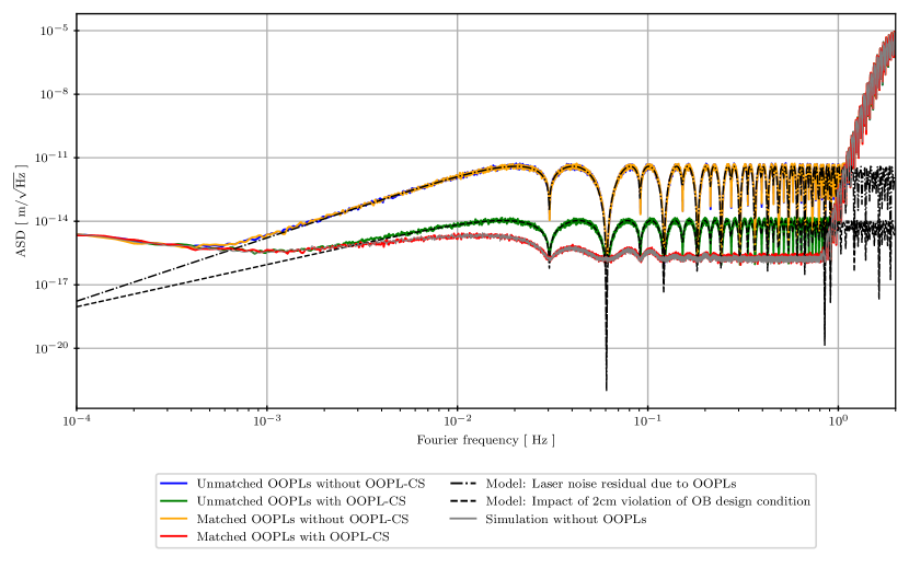
Figure 3: Residual laser noise in $X_{2}$ for three simulations with different OOPLs. Grey: Simulation without OOPLs. Blue and green: Simulation with the current design values. Orange and red: Simulation with matched OOPLs. Blue and orange: Without application of the OOPL-CS. Red and green: With the application of the OOPL-CS. Black dash-dotted: Analytical model for the laser noise residual due to OOPLs in $\mathrm{m}\text{\,}{\mathrm{Hz}}^{-0.5}$ (see eq. 92). Black dashed: Analytical model for the impact of the $2\text{\,}\mathrm{cm}$ violation of the OB design guideline in $\mathrm{m}\text{\,}{\mathrm{Hz}}^{-0.5}$ (see section IV).

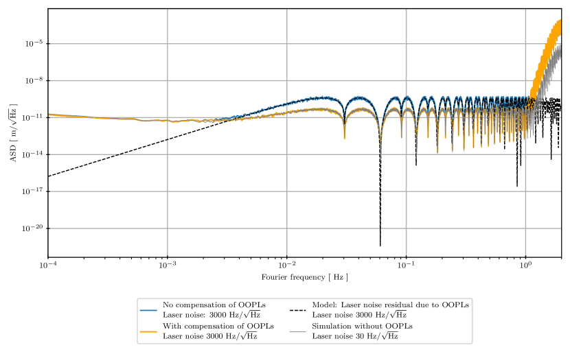
Figure 4: Simulation including secondary noises. Blue: Residual noise in $X_{2}$ for increased laser noise of $3000\text{\,}\mathrm{Hz}\text{\,}{\mathrm{Hz}}^{-0.5}$ without OOPL-CS. Orange: Residual noise in $X_{2}$ for increased laser noise of $3000\text{\,}\mathrm{Hz}\text{\,}{\mathrm{Hz}}^{-0.5}$ with OOPL-CS. Grey: Residual noise in $X_{2}$ for a simulation without OOPLs and laser noise of $30\text{\,}\mathrm{Hz}\text{\,}{\mathrm{Hz}}^{-0.5}$. Black dashed: Analytical model for the laser noise residual due to OOPLs with increased laser noise of $3000\text{\,}\mathrm{Hz}\text{\,}{\mathrm{Hz}}^{-0.5}$.

In this section, we verify and demonstrate the performance improvement due to the OOPL-CS (see section III) via numerical simulations using PyTDI [21]. We numerically assess the laser noise residuals associated with OOPLs and the impact of the $2\text{\,}\mathrm{cm}$ violation of the OB design guideline (see eq. 28). Finally, we compare the results with the analytical models derived in section IV.

We conduct two studies: In the first one (section V.1), we just consider white laser frequency noise with the ASD

$$\sqrt{S_{\dot{p}}(f)}=$30\text{\,}\mathrm{Hz}\text{\,}{\mathrm{Hz}}^{-0.5}$.$$ (94)

In the second one (section V.2), we add secondary noises and investigate the impact of increased laser frequency noise with the ASD $3000\text{\,}\mathrm{Hz}\text{\,}{\mathrm{Hz}}^{-0.5}$. In both studies, we consider telemetry data simulated with LISA Instrument [22] using an orbit file provided by ESA [19]. We do not apply laser locking. Its impact is discussed in appendix B. We neglect clock noise and clock desynchronizations. Furthermore, we assume the intersatellite ranges to be perfectly known and neglect ranging noise. A framework to obtain accurate and precise estimates for the intersatellite ranges is provided in [14].

V.1 Simulation with just laser frequency noise

We perform two simulations: In the first one, we apply the current OOPL design values (first column in table 1). In the second simulation, we consider matched OOPLs (second column in table 1), i.e., we add $2\text{\,}\mathrm{cm}$ to $d_{\text{rfi}}^{\text{adj}}$ so that eq. 28 is fulfilled exactly. In both simulations, we add manufacturing asymmetries in the order of $100\text{\,}\mathrm{\SIUnitSymbolMicro m}$ as described in appendix A. We compute the second-generation TDI X Michelson variables with and without the OOPL-CS for both simulations. For comparison, we consider a third simulation without any OOPLs.

Fig. 3 shows the corresponding ASDs as displacement noise in $\mathrm{m}\text{\,}{\mathrm{Hz}}^{-0.5}$. The steep slopes above $1\text{\,}\mathrm{Hz}$ are caused by aliasing and interpolation errors [15]. In the case of matched OOPLs, the results with and without the OOPL-CS are plotted in red and orange, respectively. The grey line shows the results of the simulation without OOPLs. For matched OOPLs, the OOPL-CS suppresses laser frequency noise by about 4 orders of magnitude (red versus orange). It reaches the performance of the simulation without OOPLs (red versus grey). The black dash-dotted line shows the analytical model for the impact of OOPLs (see eq. 92). Above $1\text{\,}\mathrm{mHz}$, it agrees with the plots for simulations without the OOPL-CS (black dash-dotted versus blue and orange), which is expected since, here, the performance is limited by exactly these OOPLs. In the low frequencies, the numerical results deviate from the model. This is due to the approximation of constant equal arms, which is violated by ESA orbits but used in modeling. Moreover, while the model only covers adjacent OOPLs in the RFI, we include the full set of OOPLs in the numerical simulations.

In the case of the current OOPL design values, the results with and without the OOPL-CS are plotted in green and blue, respectively. For these unmatched OOPLs, the OOPL-CS reduces the laser frequency noise by more than 2 orders of magnitude (green versus blue). Here, its performance is limited by the laser noise residual associated with the $2\text{\,}\mathrm{cm}$ violation of the OB design guideline. The analytical model of this $2\text{\,}\mathrm{cm}$ mismatch (see section IV) is represented by the black dashed line and agrees with the numerical result (black dashed versus green). The deviations from this model in the low frequencies are due to our usage of ESA orbits and interpolation errors in TDI (the delays are not integer multiples of the $0.25\text{\,}\mathrm{s}$ sampling time).

V.2 Simulation including secondary noises

We consider a more realistic scenario and add readout, test-mass acceleration, and backlink noise as specified in [18]. We study the impact of lasers that perform below expectations, i.e., we consider increased laser frequency noise with an ASD of $3000\text{\,}\mathrm{Hz}\text{\,}{\mathrm{Hz}}^{-0.5}$. We apply the current OOPL design values. For comparison, we perform a simulation without OOPLs and $30\text{\,}\mathrm{Hz}\text{\,}{\mathrm{Hz}}^{-0.5}$ laser noise.

Fig. 4 shows the performance of the OOPL-CS in this scenario. For the increased laser frequency noise level, we plot the results with and without the OOPL-CS in orange and blue, respectively. The grey plot shows the residual noise in $X_{2}$ for the simulation without OOPLs and the common laser noise level. It can be seen that the orange curve matches the grey one. This validates the performance of the OOPL-CS with secondary noises and for increased laser frequency noise.

The black dashed line shows the model for the impact of OOPLs with increased laser frequency noise of $3000\text{\,}\mathrm{Hz}\text{\,}{\mathrm{Hz}}^{-0.5}$. Above $4\text{\,}\mathrm{mHz}$, the laser noise residuals due to OOPLs exceed the secondary noises. Here, the model matches the simulation without OOPL-CS (blue versus black dashed). Hence, in the case of increased laser noise of $3000\text{\,}\mathrm{Hz}\text{\,}{\mathrm{Hz}}^{-0.5}$, OOPL-related laser noise residuals become the primary noise source above $4\text{\,}\mathrm{mHz}$.

VI Conclusion

TDI applies estimates for the interspacecraft distances to construct equal-optical-path-length interferometers from the LISA interferometric measurements. In a realistic LISA simulation, which does not simplify the LISA satellites as point masses, OOPLs become part of these equal-optical-path-length interferometers.

We derive an analytical model for the coupling of OOPLs in TDI (see eq. 92) depending on the laser frequency noise level and the adjacent OOPL in the RFI. This model can be of further importance for the study of underperforming lasers in LISA and for the assessment of laser requirements in next-generation space-based gravitational-wave missions. We validate this model numerically by including OOPLs in the LISA simulation [22] and compute the associated laser noise residual in the second-generation TDI Michelson variable $X_{2}$ using PyTDI [21].

We derive a compensation scheme for OOPLs (OOPL-CS), which includes OOPL delay and advancement operators in the TDI combinations. As a byproduct of the OOPL-CS, we derive a guideline for the OB design (see eq. 28): To facilitate the complete cancellation of the OOPL-related laser noise residuals in TDI, the difference between local OOPLs in the RFI and TMI has to match the difference between adjacent OOPLs in these interferometers. This should not be understood as a strict condition but rather as a guideline. The current OB design values [12] involve a mismatch of about $2\text{\,}\mathrm{cm}$. We derive an analytical model for the impact of this mismatch and verify it numerically. It is in the order of $10\text{\,}\mathrm{fm}\text{\,}{\mathrm{Hz}}^{-0.5}$ and thus negligible across the LISA band. This model can be of further importance for the OB design in next-generation space-based gravitational-wave missions.

We assess the performance of the OOPL-CS numerically. In a simulation with just laser frequency noise, we show that the OOPL-CS can completely remove the OOPL-related laser noise residuals. Furthermore, we validate the performance of the OOPL-CS in the presence of secondary noise sources and for increased laser frequency noise of $3000\text{\,}\mathrm{Hz}\text{\,}{\mathrm{Hz}}^{-0.5}$. For laser frequency noise of $30\text{\,}\mathrm{Hz}\text{\,}{\mathrm{Hz}}^{-0.5}$, the laser noise residual due to OOPLs reaches the order of $1\text{\,}\mathrm{pm}\text{\,}{\mathrm{Hz}}^{-0.5}$ but remains below the secondary noise sources. However, in the scenario of underperforming lasers, the OOPL-related laser noise residuals can compete with the secondary noises, and the OOPL-CS becomes a necessary processing step.

In our simulations, we consider six free-running lasers. In reality, the lasers are locked to each other. We discuss the impact of different laser-locking configurations considering our analytical models. From the perspective of OOPL-related laser noise residuals, we identify suitable and unsuitable locking configurations. It would be interesting to numerically assess the impact of OOPLs with locked lasers in a follow-up investigation.

Appendix A Manufacturing asymmetries

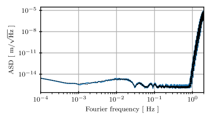
Figure 5: Impact of manufacturing asymmetries: The blue and black plots show the ASDs of $X_{2}$ for simulations with and without manufacturing asymmetries in the order of $100\text{\,}\mathrm{\SIUnitSymbolMicro m}$.

This section investigates the laser noise residuals caused by manufacturing asymmetries between the OBs. We perform two simulations according to the setup with just laser frequency noise (see section V.1). In the first simulation, we set all OOPLs to zero. In the second one, we consider manufacturing asymmetries between the OBs: We draw all OOPLs from a zero-mean Gaussian distribution with $100\text{\,}\mathrm{\SIUnitSymbolMicro m}$ as standard deviation. For both simulations, we compute the second-generation TDI X Michelson combinations. Fig. 5 shows the corresponding ASDs in $\mathrm{m}\text{\,}{\mathrm{Hz}}^{-0.5}$. The impact of manufacturing asymmetries is in the order of $1\text{\,}\mathrm{fm}\text{\,}{\mathrm{Hz}}^{-0.5}$. It is completely negligible across the LISA band.

Appendix B Laser Locking

The six LISA lasers are not independently free-running but offset frequency locked to each other according to a frequency plan [2]. [18] lists the six laser-locking configurations from the perspective of laser 12 as the primary laser. Our analytical models for the coupling of OOPLs in TDI suggest that certain laser-locking configurations naturally reduce the OOPL-related laser noise residuals.

We revisit the laser noise residuals in $X_{2}$ associated with uncompensated OOPLs in TDI step 2 (see eq. 86):

$$X^{\eta} =\frac{d_{\text{rfi}}^{\text{adj}}}{2}\left(1-2\textbf{D}^{2}+2\textbf{D}^{6}-\textbf{D}^{8}\right)\left(\ddot{p}_{12}-\ddot{p}_{13}\right),$$ (95)

$Y^{\eta}$ and $Z^{\eta}$ can be obtained via cyclic permutation of the SC indices. In these laser noise residuals, local and adjacent lasers appear with opposite signs. They, therefore, cancel each other in laser-locking configurations that lock local and adjacent lasers onto each other, assuming sufficient gain of the locking control loop. Thus, the laser-locking configurations N1-12, N3-12, and N5-12 naturally reduce the OOPL-related laser noise residuals $X^{\eta}$, $Y^{\eta}$, and $Z^{\eta}$ in the second-generation TDI Michelson variables. The locking schemes (N2-12, N4-12, N6-12), on the other hand, involve one pair of not directly locked local and adjacent lasers. Here, the OOPL-related laser noise residuals do not cancel in all three TDI channels.

We also revisit the laser noise residuals in $X_{2}$ associated with uncompensated OOPLs in TDI step 1 (see eq. 81):

$$X^{\xi}=(1-\textbf{D}^{2}-\textbf{D}^{4}+\textbf{D}^{6})$$

$$\Bigg{\{}\frac{d_{\Delta}^{\text{loc}}+d_{\Delta}^{\text{adj}}}{2}\left(1+\textbf{D}^{2}\right)\left(\ddot{p}_{13}-\ddot{p}_{12}\right)$$

$$+d_{\Delta}^{\text{loc}}\>\textbf{D}\left(\ddot{p}_{31}-\ddot{p}_{21}\right)$$

$$+d_{\Delta}^{\text{adj}}\>\textbf{D}\left(\ddot{p}_{23}-\ddot{p}_{32}\right)\Bigg{\}},$$ (96)

$Y^{\xi}$ and $Z^{\xi}$ can be obtained via cyclic permutation of the SC indices. In the first term, local and adjacent lasers appear with opposite signs. Hence, the laser-locking configurations N1-12, N3-12, and N5-12 naturally suppress its contribution. The remaining terms involve a pair of lasers on different spacecraft, which can only be locked onto each other with an inter-satellite delay. These terms, therefore, cannot be meaningfully suppressed and contribute to laser noise residuals in each laser-locking configuration.

References

• Amaro-Seoane et al. [2017] P. Amaro-Seoane, H. Audley, S. Babak, J. Baker, E. Barausse, P. Bender, E. Berti, P. Binetruy, M. Born, D. Bortoluzzi, et al., Laser interferometer space antenna, arXiv preprint arXiv:1702.00786  (2017).
• Heinzel [2018] G. Heinzel, LISA frequency planning, Tech. Rep. (LISA-AEI-INST-TN-002, 2018).
• Gerberding et al. [2013] O. Gerberding, B. Sheard, I. Bykov, J. Kullmann, J. J. E. Delgado, K. Danzmann, and G. Heinzel, Phasemeter core for intersatellite laser heterodyne interferometry: modelling, simulations and experiments, Classical and Quantum Gravity 30, 235029 (2013).
• Armstrong et al. [1999] J. Armstrong, F. Estabrook, and M. Tinto, Time-delay interferometry for space-based gravitational wave searches, The Astrophysical Journal 527, 814 (1999).
• Tinto et al. [2002] M. Tinto, F. B. Estabrook, and J. Armstrong, Time-delay interferometry for LISA, Physical Review D 65, 082003 (2002).
• Hartwig et al. [2022] O. Hartwig, J.-B. Bayle, M. Staab, A. Hees, M. Lilley, and P. Wolf, Time-delay interferometry without clock synchronization, Phys. Rev. D 105, 122008 (2022).
• Heinzel et al. [2011] G. Heinzel, J. J. Esteban, S. Barke, M. Otto, Y. Wang, A. F. Garcia, and K. Danzmann, Auxiliary functions of the LISA laser link: ranging, clock noise transfer and data communication, Classical and Quantum Gravity 28, 094008 (2011).
• Sutton et al. [2010] A. Sutton, K. McKenzie, B. Ware, and D. A. Shaddock, Laser ranging and communications for lisa, Opt. Express 18, 20759 (2010).
• Armano et al. [2016] M. Armano, H. Audley, G. Auger, J. T. Baird, M. Bassan, P. Binetruy, M. Born, D. Bortoluzzi, N. Brandt, M. Caleno, et al., Sub-femto-g free fall for space-based gravitational wave observatories: LISA pathfinder results, Physical review letters 116, 231101 (2016).
• Armano et al. [2018] M. Armano, H. Audley, J. Baird, P. Binetruy, M. Born, D. Bortoluzzi, E. Castelli, A. Cavalleri, A. Cesarini, A. Cruise, et al., Beyond the required LISA free-fall performance: new LISA pathfinder results down to 20 $\mu$ hz, Physical review letters 120, 061101 (2018).
• Otto [2015] M. Otto, Time-delay interferometry simulations for the laser interferometer space antenna,  (2015).
• Brzozowski et al. [2022] W. Brzozowski, D. Robertson, E. Fitzsimons, H. Ward, J. Keogh, A. Taylor, M. Milanova, M. Perreur-Lloyd, Z. Ali, A. Earle, et al., The LISA optical bench: an overview and engineering challenges, Space Telescopes and Instrumentation 2022: Optical, Infrared, and Millimeter Wave 12180, 211 (2022).
• Euringer et al. [2024] P. Euringer, N. Houba, G. Hechenblaikner, O. Mandel, F. Soualle, and W. Fichter, Compensation of front-end and modulation delays in phase and ranging measurements for time-delay interferometry, Physical Review D 109, 083024 (2024).
• Reinhardt et al. [2024] J. N. Reinhardt, M. Staab, K. Yamamoto, J.-B. Bayle, A. Hees, O. Hartwig, K. Wiesner, S. Shah, and G. Heinzel, Ranging sensor fusion in LISA data processing: Treatment of ambiguities, noise, and onboard delays in LISA ranging observables, Phys. Rev. D 109, 022004 (2024).
• Staab et al. [2024] M. Staab, M. Lilley, J.-B. Bayle, and O. Hartwig, Laser noise residuals in LISA from on-board processing and time-delay interferometry, Physical Review D 109, 043040 (2024).
• Staab [2023] M. B. Staab, Time-delay interferometric ranging for LISA: Statistical analysis of bias-free ranging using laser noise minimization,   (2023).
• Bayle et al. [2021] J.-B. Bayle, O. Hartwig, and M. Staab, Adapting time-delay interferometry for LISA data in frequency, Physical Review D 104, 023006 (2021).
• Bayle and Hartwig [2023] J.-B. Bayle and O. Hartwig, Unified model for the LISA measurements and instrument simulations, Physical Review D 107, 083019 (2023).
• Bayle et al. [2022a] J.-B. Bayle, A. Hees, M. Lilley, C. Le Poncin-Lafitte, W. Martens, and E. Joffre, LISA Orbits (2022a).
• Risken [1996] H. Risken, Fokker-planck equation (Springer, 1996).
• Staab et al. [2023] M. Staab, J.-B. Bayle, and O. Hartwig, PyTDI (2023).
• Bayle et al. [2022b] J.-B. Bayle, O. Hartwig, and M. Staab, LISA Instrument (2022b).