SPARE: Symmetrized Point-to-Plane Distance for Robust Non-Rigid Registration
Abstract
Existing optimization-based methods for non-rigid registration typically minimize an alignment error metric based on the point-to-point or point-to-plane distance between corresponding point pairs on the source surface and target surface. However, these metrics can result in slow convergence or a loss of detail. In this paper, we propose SPARE, a novel formulation that utilizes a symmetrized point-to-plane distance for robust non-rigid registration. The symmetrized point-to-plane distance relies on both the positions and normals of the corresponding points, resulting in a more accurate approximation of the underlying geometry and can achieve higher accuracy than existing methods. To solve this optimization problem efficiently, we propose an alternating minimization solver using a majorization-minimization strategy. Moreover, for effective initialization of the solver, we incorporate a deformation graph-based coarse alignment that improves registration quality and efficiency. Extensive experiments show that the proposed method greatly improves the accuracy of non-rigid registration problems and maintains relatively high solution efficiency. The code is publicly available at https://github.com/yaoyx689/spare.
Index Terms:
non-rigid registration, symmetrized point-to-plane distance, numerical optimization, surrogate function.1 Introduction
Given a source surface and a target surface, non-rigid registration aims to compute a deformation field that aligns the source surface with the target surface. This problem is fundamental in computer vision, with various applications such as 3D shape acquisition and tracking.
In non-rigid registration, the challenge lies in aligning two surfaces without knowing their correspondence in advance. Motivated by the ICP algorithm [1] for rigid registration, many non-rigid registration methods iteratively update the correspondence using closest point queries from the source points to the target surface, and then update the deformation by minimizing an alignment error metric between the corresponding points along with some regularization terms for the deformation field [2, 3, 4]. The quality and speed of the registration are heavily influenced by the alignment error metric. A commonly used metric is the “point-to-point” distance, measured between points on the source surface and their corresponding closest points on the target surface [5, 2, 6, 7, 3, 8, 4]. However, due to the unreliability of such correspondence, the registration may converge to a local minimum and produce unsatisfactory results. Another frequently used metric is the ”point-to-plane” distance, which measures the distance between source surface points and the tangent planes at their closest points on the target surface [9, 10, 11, 12, 13]. As the point-to-plane distance is a first-order approximation of the target surface shape around the closest point, it provides a more accurate proxy of the target shape than the point-to-point distance and enables faster alignment of the two surfaces. Despite these efforts, non-rigid registration can still be challenging and time-consuming. In the rigid registration literature, alignment error metrics that incorporate higher-order geometric properties have been utilized to achieve faster convergence than the point-to-plane distance [14, 15], but such higher-order properties are expensive to compute. Recently, a symmetrized point-to-plane metric was proposed in [16] for rigid registration. It measures the consistency between the positions and normals of each source point and its corresponding closest point, and achieves the minimal value when the pair of points lies on a second-order patch of surface [16]. When used for rigid registration, this gains similar benefits of fast convergence as registration methods that exploit second-order surface properties, but without the need for explicit computation of such properties.
In this paper, we propose SPARE, a novel method that utilizes the Symmetrized Point-to-plAne distance for Robust non-rigid rEgistration. Although the symmetrized point-to-plane distance works well on rigid-rigid registration, deploying it for non-rigid registration is a non-trivial task. First, there is a large space of point pair positions and normals that can minimize the symmetrized point-to-plane distance. While this is beneficial for rigid registration problems with a limited degree of freedom, it can be problematic for non-rigid registration: due to the excessive degrees of freedom, the symmetrized point-to-plane distance may be minimized without actually aligning the two surfaces. Secondly, in real-world applications, non-rigid registration is often carried out between surface data with noise, outliers or partial overlaps, which may lead to erroneous correspondence for closest-point queries and impact the effectiveness of the symmetrized point-to-plane distance. To address the issue of excessive degrees of freedom, we incorporate an as-rigid-as-possible regulation for the deformation into our formulation in conjunction with the symmetrized point-to-plane metric for the alignment. This not only helps the deformation field to maintain local structures of the source shape, but also reduces the degrees of freedom and restores the effectiveness of the symmetrized point-to-plane distance for non-rigid registration. In addition, to address the issue of erroneous correspondence due to noise, outliers and partial overlaps, we incorporate an adaptive weight into the symmetrized point-to-plane metric, which is computed according to the positions and normals of each point pair and automatically reduces the influence of unreliable correspondence.
As the resulting optimization problem is non-convex and highly non-linear, we devise an iterative solver that alternately updates the subsets of the variables, decomposing the optimization into simple sub-problems that are easy to solve. In particular, in each iteration we adopt a majorization-minimization strategy [17] and construct a proxy problem that minimizes a simple surrogate function that bounds the target function from above, enabling us to derive closed-form update steps that can effectively reduce the original target function. Moreover, to effectively initialize the solver and avoid undesirable local minima, we propose a strategy that uses a deformation graph [18] to roughly align the two surfaces while maintaining the structure of the source shape.
We perform extensive experiments to evaluate our method on both synthetic and real datasets. Our method outperforms state-of-the-art optimization-based and learning-based methods in terms of accuracy and efficiency. To summarize, our contributions include:
-
•
We formulate a novel optimization-based approach for non-rigid registration problem. Our formulation adopts a robustified symmetrized point-to-plane distance in conjunction with an as-rigid-as-possible regularization term, significantly enhancing the robustness and accuracy of the registration solution.
-
•
We propose an efficient alternating minimization solver for the resulting non-convex optimization problem, using a majorization-minimization strategy to derive simple sub-problems that effectively reduce the target function.
-
•
We devise an effective initialization strategy for the solver, by using a deformation graph-based coarse alignment that maintains the overall structure of the source shape.
2 Related work
In the following, we review existing works closely related to our approach. More complete overviews of non-rigid registration can be found in recent surveys such as [19, 20].
For optimization-based non-rigid registration, the alignment error metric is an important component in the formulation. Many existing methods adopt the simple point-to-point distance from the classical ICP algorithm [2, 6, 21, 22, 8]. Others use the point-to-plane distance instead [11, 23, 24, 25, 12, 26, 13], which benefits from faster convergence than the point-to-point distance albeit being more complicated to solve. Some methods utilize both metrics to complement each other [9, 7, 27, 28, 29, 30, 31]. Another class of methods, such as the coherent point drift (CPD) [32], models the sample points using Gaussian mixtures and formulates the alignment error from a probabilistic perspective [32, 33, 34, 35]. Recently, a Bayesian formulation of CPD has been proposed in [36], with further work in [37, 38] to improve its performance and accuracy. In [39], CPD is also generalized to non-Euclidean domains to improve its robustness on data with large deformations.
The performance of non-rigid registration also depends on the representation of the deformation field. A simple approach is to introduce a variable for the new position or transformation of each source point [21, 40, 3]. Such a representation provides abundant degrees of freedom to represent complex deformations, but the resulting problem is often expensive to solve due to the large number of variables. Other methods address this problem using an embedded deformation graph [18], where each source point is deformed according to the transformations associated with the nearby nodes of a small graph on the surface [6, 9, 41, 8]. This reduces the number of variables and improves computational efficiency, at the cost of less expressiveness due to the fewer degrees of freedom.
Partial overlaps can be challenging for registration methods, as the point correspondence is not well defined everywhere. Some methods address this problem by assigning individual weights to each point pair in the alignment metric to reduce the impact of erroneous correspondence [2, 6, 7]. Others apply a robust norm (such as the -norm or the Welsch’s function) to the alignment metric, which automatically reduces the contribution of point pairs that are less reliable [42, 12, 43, 30, 8].
In recent years, deep learning techniques have also been adopted to deal with challenging non-rigid registration problems. Many methods rely on supervised learning to improve the quality of the alignment. Some methods learn the correspondences between source and target surfaces from ground-truth correspondences, which helps to handle data with large deformations [44, 45, 46, 47, 48]. Others use the ground-truth positions of the deformed model as the supervision to train the network to learn the correspondences or the deformation fields [49, 45, 50]. Despite their strong capabilities, these methods rely on training data with ground-truth correspondence or deformation, which is not always easy to obtain. Some unsupervised methods that do not require ground-truth correspondence have also been proposed to address this problem [51, 52, 53]. Such methods still rely on a properly designed loss function that is minimized during training to help the network learn the registration. Recently, with the rise of neural implicit representations, some implicit representation-based models are also utilized to accomplish non-rigid registration [54, 55]. Despite the rapid progress in learning-based methods, research into optimization approaches still advances the field in a complementary way: such approaches do not rely on data and are more versatile and convenient. On the data with relatively small deformation, they can usually achieve higher accuracy. They may be used to compute the required ground-truth information for supervised learning, and they can also contribute to the knowledge of loss function design for unsupervised methods.
3 Proposed Method
Consider a source surface represented by sample points equipped with normals , and a target surface represented by sample points with normals . We assume that the neighboring relation between the source sample points in is represented by a set of edges . This representation is applicable to both meshes and point clouds: the sample points are either mesh vertices or points within a point cloud, while the edges are either mesh edges or derived from the -nearest neighbors in the point cloud. The normals can come directly from the input data, be estimated from nearby points using PCA, or calculated by averaging the normals of adjacent faces in a mesh
We aim to compute a deformation field for the source surface to align it with the target surface. In practical applications, the non-rigid registration problem is inherently challenging due to partial overlap, lack of corresponding relationships, and the presence of noise and outliers in both the source and target surfaces. To this end, we propose a novel optimization formulation for non-rigid registration, utilizing a robust symmetrized point-to-plane (SP2P) distance metric and an as-rigid-as-possible (ARAP) regularization term in the target function (Secs. 3.1 & 3.2). To efficiently solve the resulting non-convex optimization, we derive a majorization-minimization (MM) solver that decomposes it into simple sub-problems with closed-form solutions (Sec. 3.3). Furthermore, to avoid local minima and improve the solution accuracy and speed, we introduce a deformation graph-based coarse alignment to initialize our MM solver (Sec. 3.4).
3.1 Preliminary: Symmetrized Point-To-Plane Distance
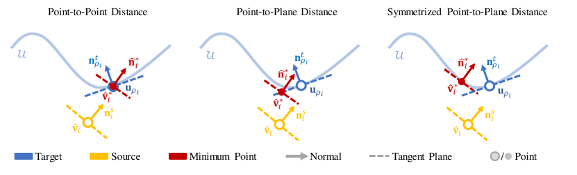
A central component for optimization-based registration is the alignment error metric that penalizes the deviation between the source surface and the target surface. Many existing non-rigid registration methods adopt a simple point-to-point metric that originates from rigid registration [1]:
| (1) |
where is the new position of after the deformation, and is the closest target point to . This allows for a simple solver that iteratively updates the closest point correspondence and re-computes the deformation according to the correspondence [2], similar to the classical ICP algorithm for rigid registration [1]. However, this metric may not accurately measure the alignment error: as the source and target point clouds may be sampled from different locations of the underlying surface, they may not fully align under the ground-truth deformation, and the point-to-point metric may not reach its minimum in this case. Moreover, the fixed closest points in each iteration fail to account for the change of correspondence for the moving source points, which can lead to slow convergence, especially when the alignment requires tangential movement along the target surface [15]. To address such issues, other methods adopt a point-to-plane metric from the rigid registration literature [56]:
| (2) |
where is the normal vector at . The metric penalizes the deviation from the tangent planes at the closest target points. Since the tangent plane is a first-order approximation of the target surface around the closest point, this metric helps to account for the target surface shape away from the sample points and leads to faster convergence than the point-to-point metric [15]. In the rigid registration literature, alignment error metrics that encode higher-order geometric properties (such as local curvatures) have also been adopted for even faster convergence than the point-to-plane metric [14, 15]. However, such higher-order properties can be expensive to compute.
To achieve faster convergence than the point-to-plane distance without evaluating higher-order properties, a symmetrized point-to-plane (SP2P) metric has been proposed recently in [16] for rigid registration:
| (3) |
where is the normal at the point on the deformed surface. Here, the term vanishes when the corresponding point pair and their normals are consistent with a locally quadratic surface centered between them [16]. In other words, the metric can be considered as penalizing the deviation between the deformed source point and a family of quadratic approximations of the target surface that are consistent with the corresponding target point and its normal . It has been observed in [16] that the symmetrized point-to-plane metric (3) leads to faster convergence of ICP than the point-to-plane metric (2).
3.2 Non-rigid Registration with Robust SP2P Distance
In this paper, we adopt the SP2P distance in Eq. (3) to propose a new optimization formulation for non-rigid registration, to benefit from its fast convergence. However, in real-world applications, the closest-point correspondence can become unreliable due to partial overlap, noise, outliers, and large initial position differences in the input surfaces. In such cases, the error metric on unreliable point pairs may steer the optimization toward an erroneous alignment. One common solution is to use dynamically adjusted weights for individual source points to control their contribution to the alignment energy based on the reliability of their correspondence [57]. Following this idea, we introduce a weighted alignment term for the source point as
| (4) |
where the weight is computed based on the deformed position , the corresponding point , and their normals in the previous iteration:
| (5) |
where is a user-specified parameter. We set to the median Euclidean distance from the initial source points to their closest target points. The weight has a large value only if both the positions and normals of the point pair are close to each other, thus reducing the influence of unreliable correspondence.
Another challenge in using the SP2P metric for non-rigid registration is that although it works well for rigid registration, using it alone for non-rigid registration is usually insufficient to achieve good results. This is because compared to the point-to-point and point-to-plane metrics, the SP2P metric has a much larger space of position and normal values with a zero metric value: on the zero level set, the positions and normals of the point pair are only required to be consistent with a certain quadratic surface patch, but the quadratic patch is not necessarily consistent with the target surface. This is not an issue for rigid registration: since all the source points must undergo the same rigid transformation, this induces an implicit regulation for the deformed source points and their normals, forcing them to align with the target surface eventually. In non-rigid registration, however, different source points may be subject to different deformations, and additional regularization terms are needed to ensure the resulting deformation field is well-behaved. In many non-rigid registration problems such as human body tracking, the surface exhibits local rigidity during deformation. Therefore, we introduce for each source point an as-rigid-as-possible (ARAP) term similar to [58], to require the deformation in its local neighborhood to be close to a rigid transformation:
| (6) |
Here is the index set of neighboring points for , and is an auxiliary rotation matrix variable for a rigid transformation associated with the source point (i.e., it needs to satisfy and ). Using the auxiliary rotation matrix , we also determine the normal of after the deformation as
| (7) |
so that the alignment term in Eq. (4) becomes
| (8) |
We will see later that the auxiliary rotation matrix enables us to devise efficient numerical solvers for the optimization problems.
3.3 Numerical Solver
The optimization problem (10) is challenging due to the non-linearity, non-convexity, and constraints of rotation matrices. To solve it efficiently and effectively, we devise an iterative solver that alternately updates the closest points , the position variables , and the rotation matrix variables while fixing the remaining variables. We denote their values after the -th iteration as , , and , respectively. In the following, we explain how to update their values in the (+1)-th iteration.
Update of . Following the solver in [16], we fix the source point positions and update closest points via
| (11) |
Afterward, we also compute the updated robust weights according to Eq. (5).
Update of . After updating , we fix the closest points , rotations , and robust weights , and minimize the target function in Eq. (10) with respect to . This problem can be written in a matrix form:
| (12) |
where concatenate and respectively. The specific forms of other variables can be found in Appx. A.1. Then the problem in Eq. (12) can be solved via a linear system
| (13) | ||||
As the system matrix is sparse, symmetric, and positive definite, we solve it using Cholesky factorization. Moreover, the sparsity pattern of the matrix remains the same in each iteration. Thus, to improve efficiency, we perform symbolic factorization once before the first iteration, and only carry out numerical factorization in each iteration.
Update of . Finally, we update the rotation matrices by fixing and and minimizing the target function with respect to . This is reduced to an independent sub-problem for each :
| s.t. | (14) |
where . As far as we are aware, there is no closed-form solution to this problem. For an efficient update, we adopt the idea of majorization-minimization (MM) [17] and minimize a convex surrogate function that is constructed based on the current variable value . The surrogate function should bound the original target function from above and have the same value as at , i.e.,
| (15) | ||||
As a result, the minimizer of is guaranteed to decrease the original target function compared to , unless is already a local minimum of (in which case the minimizer of will be exactly ) [17]. In the following, we will derive a simple surrogate function that allows for a closed-form solution, enabling fast and effective update of .
Proposition 1.
If , then in Eq. (16) satisfies
| (17) |
where is a plane containing all vectors that satisfy
| (18) |
i.e., is the squared distance from to the plane , scaled by a factor .
Proof.
Based on Eq. (17), we can construct a surrogate function for at the variable value as:
| (22) |
where is the closest projection of onto the plane , i.e., (see Appx. A.2 for a proof that satisfies the conditions of a surrogate function). It is easy to show that can be computed as
| (23) |
By replacing with its surrogate function in Eq. (22), we replace the optimization problem (14) with the following proxy problem:
| s.t. |
This problem has a closed-form solution [59]:
| (24) |
where the matrices , are from the SVD
for the matrix
| (25) | ||||
where . Note that although the above derivation is based on Proposition 1 which requires , the solution in Eq. (24) remains effective when : in this case, the target function in (14) reduces to
and the matrix in Eq. (25) becomes
Then the matrix in Eq. (24) is exactly the solution to the reduced optimization problem [59]. Later in Sec. 4.3, we will showcase the benefits of this solution for updating .
Termination criteria. We stop the iteration if at least one of the following conditions is satisfied: (1) the norm of the point position changes in an iteration is less than a threshold, i.e., , where is a user-specified parameter (we set in our experiments; (2) the number of iterations reaches an upper bound (we set ). Algorithm 1 summarizes our solver for the optimization problemin Eq. (10).
3.4 Coarse Alignment Using a Deformation Graph
Our numerical solver presented in Sec. 3.3 is a local solver that searches for a stationary point near the initial solution. Therefore, proper initialization is crucial for achieving desirable results. To this end, we initialize the solver with a coarse alignment computed using a deformation graph [18]. The deformation graph controls the source surface shape with a reduced number of variables, allowing us to efficiently determine a deformation that roughly aligns the two surfaces while preserving the structure of the source shape.
Specifically, to construct a deformation graph, we follow [4] and first uniformly sample a subset from as the deformation graph nodes, so that the number of nodes is much smaller than the number of source points. Next, we establish an edge set by connecting the neighboring nodes, thereby deriving a deformation graph . We then assign to each node an affine transformation, represented by a matrix and a vector . The transformations at the nodes determine the deformation of each source point as
| (26) |
where is the node set that affects , with denoting the geodesic distance and being the sampling radius. We set by default, where is the average edge length of the source surface. The weight for the influence of on is defined as [4]:
The target function is a combination of the following terms:
-
•
Alignment and ARAP terms. We use an alignment term and an ARAP term similar to the ones presented in Sec. 3.2 but with two main differences: (1) the deformed source point position is computed from the deformation graph according to Eq. (26); (2) as only a rough alignment is needed, we apply the alignment term only to a sampled subset of the source points to reduce computation, i.e.,
(27) where is defined in the same way as Eq. (4). By default, we set the number of sampling points to 3000.
-
•
Other regularization terms. To ensure the deformation graph induces a smooth deformation that preserves the structure of the source shape, we introduce two additional regularization terms from [4]. First, we use the following term to enforce the smoothness of the transformations across the deformation graph:
(28) where is the difference of the graph node deformed by the affine transformations and and calculated by
and is a normalization weight. In addition, we use the following term to require the affine transformation associated with each node to be close to a rigid transformation:
(29) where is the projection operator and is the rotation matrix group. Compared to the ARAP term, enforces local rigidity at a larger scale and helps to maintain the structure of the source shape. Further details of these two terms can be found in [4].
Using these terms, our optimization problem for coarse alignment can be written as
| (30) |
where are auxiliary rotation matrix variables for the alignment and ARAP terms. Similar to Sec. 3.3, we solve this problem by alternating updates of the variables using an MM strategy. Details of the solver can be found in Appx. A.3.
4 Results
We conducted comprehensive performance comparisons of the proposed method with the state-of-the-art non-rigid registration methods. In addition, we evaluated the effectiveness of the components in our formulation. This section provides details of our experiment settings and results.
4.1 Experiment settings
To assess the effectiveness and accuracy of our method, we conducted comparisons with several existing methods: the non-rigid ICP method (N-ICP) from [2]; the Welsch function-based formulation from [4] (AMM); the Bayesian Coherent Point Drift method (BCPD) [36] and its variants BCPD++ [37] and GBCPD/GBCPD++ [38]. Additionally, we compared our method with state-of-the-art learning-based methods, including LNDP [61], SyNoRiM [62], and GraphSCNet [48]. The comparisons were performed using the open-source implementations of these methods111https://github.com/Juyong/Fast_RNRR,222https://github.com/yaoyx689/AMM_NRR,333https://github.com/ohirose/bcpd,444https://github.com/rabbityl/DeformationPyramid,555https://github.com/huangjh-pub/synorim,666https://github.com/qinzheng93/GraphSCNet. All methods were evaluated using a synthetic dataset, the DeformingThings4D (DT4D) dataset [63], and real datasets including the articulated mesh animation (AMA) dataset [60] and the SHREC’20 Track dataset [64]. Additionally, we assessed all optimization-based methods using real datasets including DFAUST [65], DeepDeform [45] and the face sequence from [27], to test their effectiveness for non-rigidly tracking. For each dataset, we tuned the parameters of each optimization-based method to achieve the best overall performance. For learning-based methods, we used the pre-trained models provided by the authors for testing. Detailed parameter settings can be found in Appx. B.
The experiments were conducted using a PC equipped with 32GB of RAM, a 6-core Intel Core i7-8700K CPU at 3.70GHz, and an NVIDIA GeForce RTX 2080Ti GPU. They were all running on Ubuntu 20.04 LTS system built with Docker. All optimization-based methods leveraged multi-thread acceleration on the CPU, while learning-based methods utilized CUDA acceleration on the GPU. For all problem instances, we scaled the source surface and target surface with the same scaling factor, such that the two surfaces are contained in a bounding box with a unit diagonal length to test all comparison methods. To have a clear error scale, we rescale the model to its original size and calculate the error in meters. In the subsequent presentation of numerical results in tables, we highlight the best results using bold fonts, while underlining the second-best results for clarity and emphasis. In all result figures, we render the target surface in yellow, while the source surface and the deformed surface are rendered in blue.
4.2 Comparison with State-of-the-Art Methods
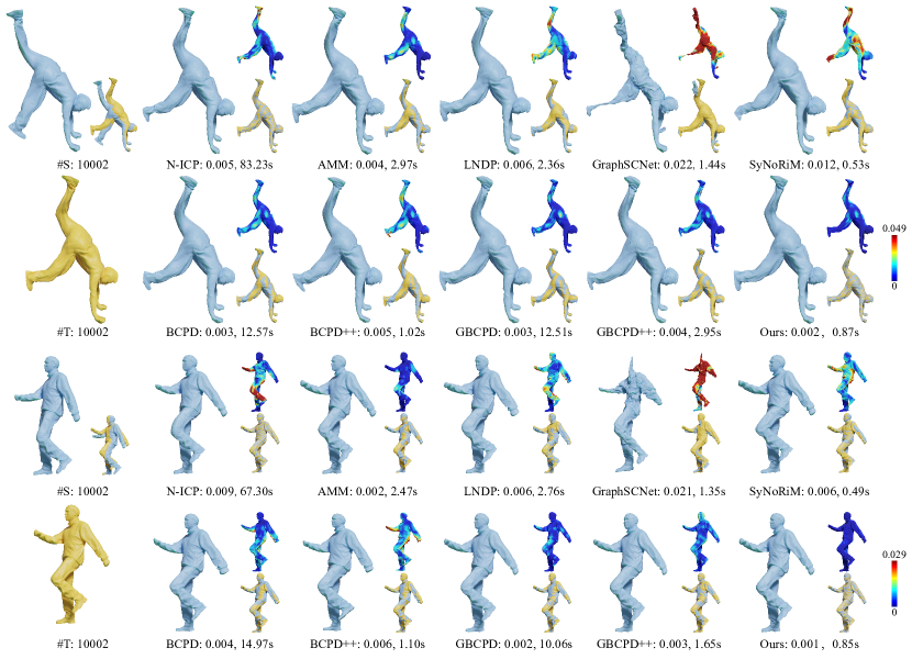
Clean data. We evaluated different registration methods using the AMA dataset [60] to assess their performance in continuous sequence scenarios. The dataset consists of 10 sequences of human continuous motion captured from real-world scenarios, and data have been processed into triangular meshes with the same connectivity structure in each sequence. Following [4], we focused on the “handstand” and “march1” sequences from [60]. For each sequence, we selected 50 pairs of models to test, considering the -th mesh as the source model and the (+2)-th mesh as the target model, where . Since the AMA dataset provides the ground-truth position for each point, we utilize the root-mean-square error to measure the registration error:
| (31) |
where is the ground-truth positions for . Since the registered surface may match the target model surface very well, but is not aligned with each target point, RMSE cannot fully reflect the quality of registration. Therefore, we also measure the point-to-plane distances between each deformed point and its corresponding ground truth position. That is
| (32) |
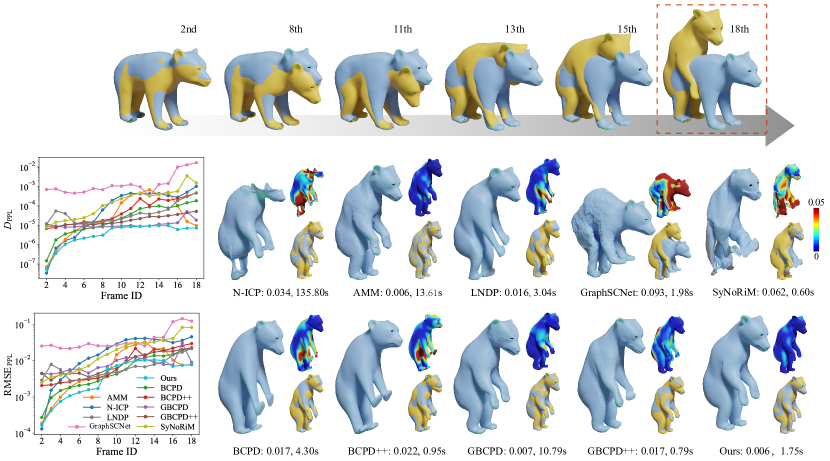
where denotes the normal of . In Tab. I, we present the average values of RMSE, RMSE and average computation time for each sequence. Additionally, we provide visualizations of two specific cases in Fig. 2. From the results, it can be observed that our method achieves the smallest values for both RMSE and RMSE among all compared methods. Furthermore, the average computation time of our method is the second shortest and only longer than SyNoRiM, which is a learning-based method with GPU acceleration.
| Method | handstand | march1 | ||
| RMSE | Time | RMSE | Time | |
| N-ICP [2] | 3.03 / 1.47 | 66.58 | 1.67 / 0.82 | 39.84 |
| AMM [4] | 1.19 / 0.67 | 2.35 | 0.70 / 0.39 | 1.51 |
| BCPD [36] | 1.29 / 0.69 | 4.97 | 1.18 / 0.58 | 5.40 |
| BCPD++ [37] | 1.71 / 0.88 | 3.21 | 1.74 / 0.86 | 3.33 |
| GBCPD [38] | 1.14 / 0.62 | 10.07 | 0.55 / 0.31 | 9.53 |
| GBCPD++ [38] | 1.46 / 0.73 | 2.68 | 1.08 / 0.51 | 2.38 |
| GraphSCNet [48] | 9.44 / 5.62 | 1.95 | 7.23 / 4.46 | 1.85 |
| LNDP [61] | 2.23 / 1.20 | 1.90 | 1.85 / 1.02 | 1.43 |
| SyNoRiM [62] | 3.20 / 1.63 | 0.54 | 2.20 / 1.10 | 0.48 |
| Ours | 0.86 / 0.40 | 0.96 | 0.26 / 0.11 | 0.80 |
| Method | 1 (76.30) | 2 (73.55) | 3 (70.94) | 4 (67.98) | 5 (64.43) | 6 (60.71) | 7 (56.60) | 8 (52.50) | 9 (48.61) |
| N-ICP [2] | 0.27 / 0.11 | 0.30 / 0.12 | 0.34 / 0.14 | 0.33 / 0.13 | 0.31 / 0.12 | 0.31 / 0.13 | 0.32 / 0.14 | 0.36 / 0.16 | 0.37 / 0.17 |
| AMM [4] | 0.10 / 0.05 | 0.11 / 0.05 | 0.13 / 0.06 | 0.12 / 0.05 | 0.13 / 0.06 | 0.11 / 0.05 | 0.14 / 0.06 | 0.16 / 0.08 | 0.20 / 0.10 |
| BCPD [36] | 0.84 / 0.41 | 0.97 / 0.49 | 1.17 / 0.57 | 1.34 / 0.69 | 1.30 / 0.66 | 1.28 / 0.67 | 1.49 / 0.80 | 1.52 / 0.83 | 1.59 / 0.89 |
| BCPD++ [37] | 0.47 / 0.27 | 0.57 / 0.33 | 0.64 / 0.35 | 0.67 / 0.36 | 0.64 / 0.36 | 0.62 / 0.36 | 0.83 / 0.49 | 0.91 / 0.55 | 1.02 / 0.60 |
| GBCPD [38] | 0.99 / 0.48 | 1.23 / 0.61 | 1.48 / 0.73 | 1.42 / 0.68 | 1.38 / 0.69 | 1.30 / 0.65 | 1.41 / 0.71 | 1.54 / 0.79 | 1.55 / 0.82 |
| GBCPD++ [38] | 0.90 / 0.44 | 1.07 / 0.53 | 1.27 / 0.63 | 1.21 / 0.61 | 1.19 / 0.60 | 1.14 / 0.59 | 1.26 / 0.64 | 1.38 / 0.73 | 1.43 / 0.78 |
| GraphSCNet [48] | 1.34 / 0.67 | 1.40 / 0.71 | 1.58 / 0.78 | 1.55 / 0.75 | 1.54 / 0.73 | 1.32 / 0.64 | 1.44 / 0.68 | 1.44 / 0.70 | 1.32 / 0.68 |
| LNDP [61] | 1.31 / 0.63 | 1.55 / 0.74 | 1.89 / 1.04 | 2.18 / 1.05 | 2.13 / 1.17 | 1.54 / 0.87 | 2.21 / 1.28 | 2.56 / 1.43 | 1.72 / 1.06 |
| SyNoRiM [62] | 0.51 / 0.25 | 0.61 / 0.30 | 0.84 / 0.45 | 0.77 / 0.41 | 1.01 / 0.62 | 1.06 / 0.64 | 0.97 / 0.55 | 1.10 / 0.64 | 1.36 / 0.71 |
| Ours | 0.08 / 0.04 | 0.09 / 0.04 | 0.11 / 0.05 | 0.09 / 0.04 | 0.08 / 0.03 | 0.08 / 0.03 | 0.08 / 0.03 | 0.10 / 0.05 | 0.09 / 0.04 |
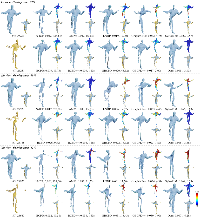
Partial overlaps. In practice, many non-rigid registration problems involve surface pairs with partial overlaps that increase the difficulty of registration. To evaluate the methods on such data, we used the “crane” sequence from the AMA dataset [60] as test cases. We first selected ten pairs of meshes from the crane sequence, each consisting of two adjacent frames in the sequence. For each mesh pair, we derived nine pairs of point clouds by simulating depth cameras from a fixed view angle for the source mesh , and from nine different view angles for angle for the target mesh with increasing deviation from the source view angle. This results in nine pairs of point clouds for each mesh pair, with decreasing overlap ratios. we report the average values of the following overlap ratio for all pairs using the same view angles:
| (33) |
where is ’s position under the ground-truth deformation, is the closest target point to , and is the average distance between neighboring points on the target shape. That is, represents the proportion of source points whose distance to the target shape, under the ground-truth deformation, is smaller than a threshold related to the sampling density.
Next, we applied non-rigid registration methods to all point cloud pairs, and calculated the average values among all point clouds for two metrics, RMSE and RMSE, which measure the root-mean-square errors with the point-to-point and point-to-plane distance respectively for the ground-truth correspondences between the source and target models:
| (34) | ||||
where is the set of ground-truth correspondence pairs, including all in the overlapping area defined by Eq. (33). Tab. II and Fig. 3 present the comparison results for the registration performance. Due to the small deformation differences in these data, with almost no detail deformation and low overlap, we only employed coarse alignment to better preserve the shape of the source surface in the deformed model. Based on the results shown in Tab. II and Fig. 3, it is evident that the proposed method achieved the highest matching accuracy among all the compared methods.
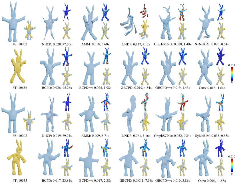
In addition, we utilized the models from the SHREC’20 dataset [64] to evaluate the performance of the registration methods. The dataset consists of a complete mesh and 11 partial meshes of a real-world object, where the partial meshes exhibit diverse shapes with fine details, resulting from different deformations (stretch, indent, twist and inflate) and different filling materials. We considered the full mesh as the source surface, and the partial meshes as the target surfaces. This dataset provides sparse ground-truth correspondences, we treat them as the elements of to calculate RMSE and RMSE according to Eq. (34) To further evaluate the errors of dense points, we calculate the point-to-point distance and the point-to-plane distance from the partial meshes to the deformed source surfaces:
where and are the position and normal of the closest point to . Tab. III shows the numerical results, and Fig. 4 visualizes two specific cases. We can see that our proposed method achieves notably higher accuracy compared to other methods in the evaluation. This superior performance can be attributed to the high degrees of freedom provided by our dense deformation field, as well as the reweighting scheme that can effectively handle partial overlaps. Moreover, our method achieves the best speed among optimization-based methods, and only falls behind the GPU-accelerated learning-based methods SyNoRiM and GraphSCNet.
| Method | Time | ||||
| N-ICP [2] | 66.43 | 37.12 | 3.60 | 1.89 | 79.59 |
| AMM [4] | 16.81 | 13.05 | 2.11 | 1.16 | 5.95 |
| BCPD [36] | 6.81 | 4.56 | 3.42 | 1.65 | 16.80 |
| BCPD++ [37] | 10.11 | 6.70 | 2.88 | 1.43 | 2.05 |
| GBCPD [38] | 1.07 | 0.58 | 2.01 | 1.04 | 7.17 |
| GBCPD++ [38] | 1.12 | 0.56 | 2.15 | 1.07 | 1.84 |
| GraphSCNet [48] | 37.10 | 23.99 | 4.48 | 2.36 | 1.59 |
| LNDP [61] | 203.71 | 114.46 | 15.48 | 7.53 | 3.06 |
| SyNoRiM [62] | 47.03 | 28.27 | 9.15 | 4.68 | 0.54 |
| Ours | 0.41 | 0.10 | 1.48 | 0.84 | 1.69 |
| Method | hips | jiggle-on-toes | jumping-jacks | chicken-wings | ||||||||
| RMSE | RMSE | Time | RMSE | RMSE | Time | RMSE | RMSE | Time | RMSE | RMSE | Time | |
| N-ICP [2] | 3.70 | 1.93 | 8.54 | 1.73 | 0.84 | 12.21 | 10.16 | 4.87 | 14.18 | 4.74 | 2.45 | 14.29 |
| AMM [4] | 0.97 | 0.47 | 2.18 | 0.93 | 0.49 | 2.60 | 4.50 | 2.11 | 4.51 | 2.49 | 1.27 | 4.32 |
| BCPD [36] | 73.11 | 39.88 | 34.31 | 77.24 | 37.97 | 22.11 | 84.56 | 42.03 | 34.27 | 74.53 | 41.89 | 46.46 |
| BCPD++ [37] | 57.98 | 33.07 | 3.63 | 77.23 | 38.45 | 2.86 | 80.28 | 40.20 | 3.77 | 51.77 | 27.37 | 5.84 |
| GBCPD [38] | 59.75 | 33.17 | 13.71 | 79.39 | 38.56 | 12.32 | 83.90 | 42.01 | 13.66 | 55.22 | 32.58 | 14.10 |
| GBCPD++ [38] | 53.08 | 26.66 | 1.45 | 44.95 | 18.62 | 1.45 | 35.56 | 16.83 | 1.38 | 36.85 | 18.34 | 1.62 |
| Ours | 0.55 | 0.28 | 0.53 | 0.92 | 0.46 | 0.58 | 3.51 | 1.81 | 0.64 | 2.11 | 1.13 | 0.63 |
Large deformation. To verify the robustness of our method to the magnitude of deformation, we conducted evaluations using data with gradually increasing deformation differences. Specifically, we selected a sequence (bear3EP_Agression) from the DT4D dataset [63] to test our method. This is a synthetic dataset that includes continuous motion sequences of various animals and humanoids. The shapes in each sequence are represented as triangular meshes with the same connectivity structure. We set the first mesh as the source model and the -th mesh as the target model (=2,…,18) for this sequence. We calculate the according to Eq. (32) and the bidirectional point-to-plane distance
between the deformed model and the target model and show them in Fig. 5. From the figure, we can observe that our method obtains the best accuracy from the 3rd frame to the 8th frame, while the RMSE in other frames is slightly worse than some methods. This is because our method can make the deformed model slide on the surface, resulting in offsets between the deformed points and the ground-truth corresponding points. From bidirectional point-to-plane distances and rendered figures, we can also see that our method is more accurate or similar in matching geometric surfaces.
Non-rigid tracking. To evaluate the practicality of the proposed method, we conducted non-rigid tracking experiments on real-world data, including the DFAUST dataset [65], the DeepDeform dataset [45] and the face sequence from [27]. For a real scan sequence , we choose a template model , and register it to and obtain the deformed model . Then we deform to align with () and obtain a mesh sequence aligned with . Due to the accumulation of errors in the registration process, this setting increases the difficulty of the problem and makes it easier to demonstrate the performance of different methods. Since there is usually a small difference between two adjacent frames, it is generally solved using optimization-based methods. We ignore the comparisons with learning-based methods in these examples.
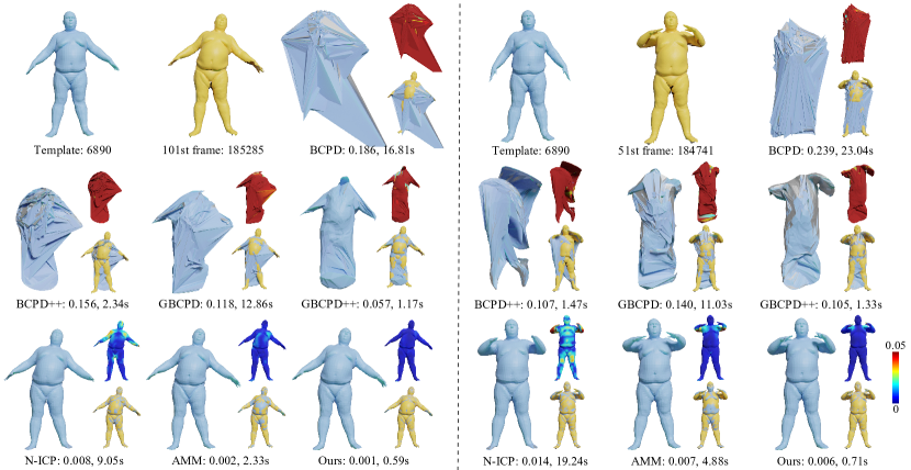
The DFAUST dataset contains multiple continuously moving human scans and the corresponding template mesh obtained by the skinned multi-person linear model (SMPL) [66]. We utilized the template mesh from the SMPL model matching the first frame as , and deformed it to align the following -th human scan, where . We also used the template meshes of SMPL model matched to these scans as the ground-truth meshes. We chose four sequences: “hips”, “jiggle-on-toes”, “jumping-jacks” and “chicken-wings” of the identity labeled as 50002 to test, where the deformations of the latter two sequences are much larger than those of the first two sequences. We compute RMSE and RMSE between the registered results with the ground-truth meshes, and show their average values and the average running time in Tab. IV. We also provide visualizations of two cases in Fig. 6.
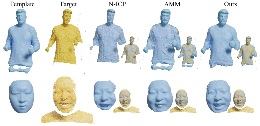
The face sequence from [27] is represented as depth maps and captures facial expressions and muscle movements, which were acquired using a single depth sensor. We utilized the provided template model from [27] as the template model , and deformed it to align with the continuous point clouds, which were obtained by converting depth maps.
The DeepDeform dataset [45] is a real RGB-D video dataset, including various scenes such as humans, clothes, animals, etc. Since it does not provide well-defined template meshes, we selected a motion sequence of a human, adopted the reconstructed mesh from [55] as the template mesh and deformed it to align the point clouds converted from the depth maps. Due to the significant difference in pose between the template model and the first scan , we manually align rigidly to before the non-rigid registration. Since these two datasets have no ground-truth information, and the data tested for non-rigid registration are partially overlapping and contain noises or outliers. We show the 2 cases of registration results in Fig. 7. Since the BCPD-class methods are too ineffective, we omit its results. We can observe that the proposed method is significantly better than other methods. It shows that our method can perform non-rigid registration more stably and reliably. To more intuitively show the performance, we also render the frame-by-frame rendering results of different methods for these three datasets in the Supplementary Video.
4.3 Effectiveness of Components
To measure the effectiveness of different components in our method, we conducted experiments by either removing a specific term or replacing it with an existing method. We compared these variants on the AMA dataset [60] with small differences (“handstand” and “march1” sequence in Tab. I) and partial overlaps (“crane” sequence in Tab. II). For the “crane” sequence, we present representative perspectives (3rd and 7th views). We also performed comparisons on the SHREC’20 non-rigid correspondence dataset [64] and the DT4D dataset [63]. We show all numerical comparisons in Tab. V and visualized results in Figs. 8,9,10,11.
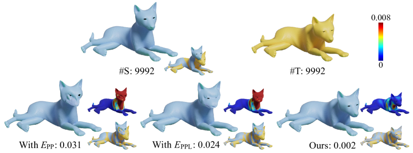
Effectiveness of symmetrized point-to-plane distance. We replaced the symmetrized point-to-plane distance metric in our target function by the point-to-point distance metric (With ) and the point-to-plane distance metric (With ) respectively while keeping other components and the reliable weights the same. From Tab. V, we observe that the symmetrized point-to-plane distance achieves better results than the variants based on and . We also show a test case on the DT4D dataset [63], which has more obvious visual differences due to its relatively large deformation.
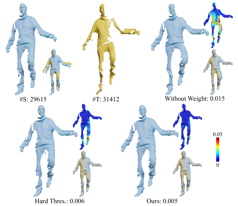
Effectiveness of the robust weights. Moreover, to test the effectiveness of the adaptive robust weights, we compared with the following strategies:
-
•
Without Weight: setting for all and (i.e., no weight);
-
•
Hard Thres.: setting
(35) i.e., a hard thresholding of the weight based on the distance between the corresponding points.
From Tab. V and Fig. 10, we can observe that our method with robust weights achieves the highest accuracy. Especially on partially overlapping data (the last two columns in the table), our method obtains obvious advantages.
| Variants | Coarse stage | Fine stage | Robust Weights | AMA dataset [60] | SHREC’20 [64] | Partial data from [60] | ||||||
| handstand | march1 | 3 | 7 | |||||||||
| Without ARAP | ✓ | ✓ | ✓ | ✓ | 2.89 / 1.50 | 2.27 / 1.18 | 2.69 / 1.42 | 1.72 / 0.79 | 1.62 / 0.71 | |||
| Without Smo. | ✓ | ✓ | ✓ | ✓ | 1.43 / 0.75 | 0.41 / 0.20 | 1.63 / 0.91 | 1.14 / 0.52 | 0.80 / 0.35 | |||
| Without Rot.Mat. | ✓ | ✓ | ✓ | ✓ | 1.36 / 0.71 | 0.40 / 0.19 | 1.65 / 0.92 | 0.99 / 0.49 | 0.93 / 0.42 | |||
| Coarse | ✓ | ✓ | ✓ | ✓ | ✓ | 1.41 / 0.74 | 0.41 / 0.20 | 1.63 / 0.91 | 1.13 / 0.51 | 0.78 / 0.35 | ||
| Fine | ✓ | ✓ | ✓ | 1.84 / 0.97 | 1.05 / 0.54 | 1.74 / 0.96 | 1.70 / 0.83 | 1.21 / 0.57 | ||||
| With | ✓ | ✓ | ✓ | ✓ | ✓ | 5.42 / 2.91 | 2.26 / 1.14 | 2.67 / 1.34 | 2.90 / 1.40 | 2.71 / 1.27 | ||
| With | ✓ | ✓ | ✓ | ✓ | ✓ | 1.18 / 0.58 | 0.44 / 0.20 | 1.77 / 0.97 | 1.34 / 0.63 | 1.60 / 0.66 | ||
| Without Weight | ✓ | ✓ | ✓ | ✓ | ✓ | ✓ | 1.94 / 0.96 | 0.97 / 0.52 | 1.96 / 1.09 | 36.26 / 28.71 | 9.06 / 3.92 | |
| Hard Thres. | ✓ | ✓ | ✓ | ✓ | ✓ | ✓ | Eq. (35) | 1.03 / 0.51 | 0.66 / 0.34 | 1.82 / 1.01 | 4.58 / 1.51 | 1.50 / 0.65 |
| Ours | ✓ | ✓ | ✓ | ✓ | ✓ | ✓ | ✓ | 0.86 / 0.40 | 0.26 / 0.11 | 1.48 / 0.84 | 1.33 / 0.70 | 0.87 / 0.39 |
Effectiveness of different terms and coarse alignment. Furthermore, we conducted experiments to evaluate the performance of the proposed method when only the initial alignment is used (i.e. Coarse) or when no coarse alignment is used (i.e. Fine). For the coarse stage, we also examined the impact of omitting each regularization term:
-
•
Without ARAP: we utilized only the coarse stage deformation and did not incorporate the term. In this case, the calculation of the normal after deformation in Eq. (7) was replaced by being estimated from the current iteration points .
-
•
Without Smo.: we utilized only the coarse stage deformation and did not incorporate the term;
-
•
Without Rot.Mat.: we utilized only the coarse stage deformation and did not incorporate the term.
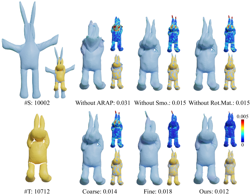
We observe that the ARAP constraint played the most crucial role. It ensured the stability of the deformation, while the smoothness term and the rotation matrix term also contributed to maintaining a coherent and well-behaved deformation. Although there was some loss in accuracy, the overall effect was more reliable. For the fine stage, when the ARAP term was not used, the absence of regularization led to deformations concentrating on specific points, resulting in poor registration results. So we omitted its results. Overall, the coarse stage focuses on matching the basic shape, while the fine stage aims to capture local details. The combination of both stages yields superior results. However, we also observe that for the constructed partially overlapping data (the last two columns in Tab. V), utilizing only the coarse stage with the deformation graph maintained the local shape more effectively. When using detailed alignment, the lack of global constraints may cause small offsets in points without correspondences. Therefore, when the overlap rate is low and the differences in detail are minimal, registration with only the coarse alignment is sufficient. Fig. 9 presents the rendering results for one of these cases.
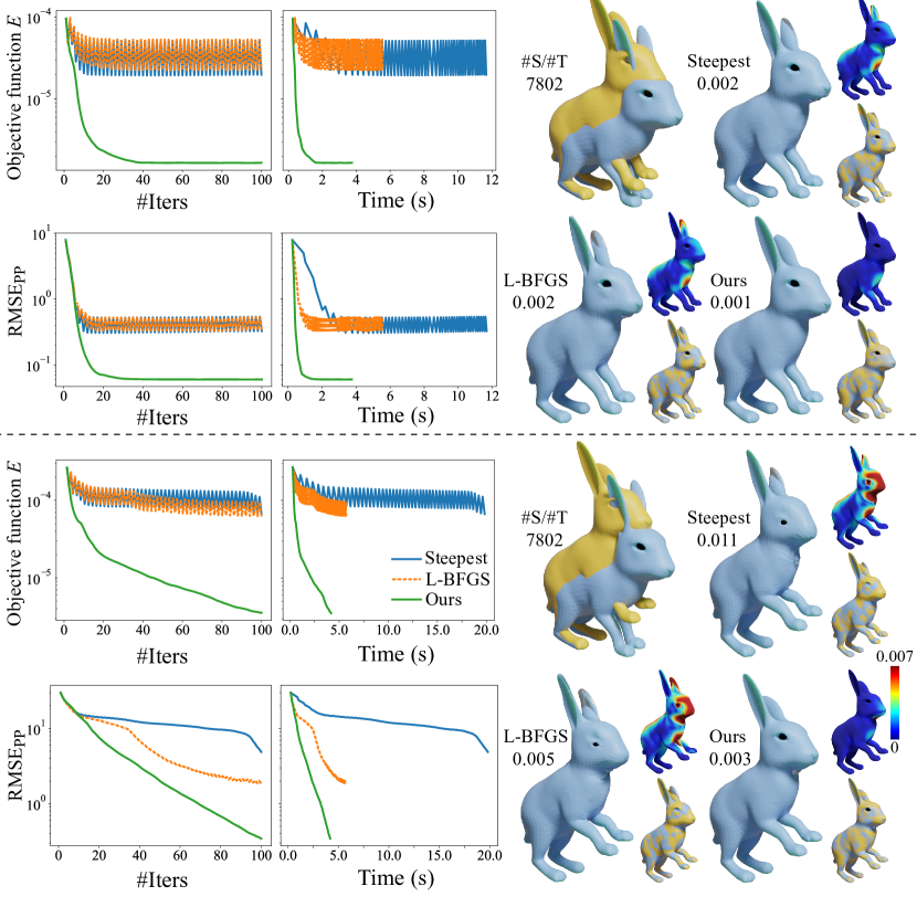
Efficiency of solving algorithms. To validate the effectiveness of our proposed solution for updating in the optimization problem (14), we compared it with gradient-based solvers that directly optimize the problem in (14) by the iterative gradient-based optimization method: the steepest descent method and the L-BFGS algorithm. Since needs to be in the rotation space, we transformed them in Lie algebra space and solved them accordingly. Specifically, we replaced with via Rodrigues’ rotation formula
| (36) |
where
and . By utilizing the transformed variables as independent variables and removing the equality constraint in problem (14), we can convert it into an unconstrained optimization problem. This allows us to employ optimization algorithms such as the steepest descent method or the L-BFGS algorithm to solve it. To ensure optimal convergence of the algorithm, we set a maximum limit of iterations for solving each sub-problem of . Additionally, the algorithm is terminated prematurely if the difference in objective function values between two consecutive iterations falls below a threshold of . To eliminate potential discrepancies caused by adaptive weights, we set for any and in this part. Fig. 11 displays the curves depicting the changes in the objective function values in Eq. (10) and RMSE over the iterations or time. Due to the high degree of nonlinearity of the problem, gradient-based optimization methods are susceptible to getting trapped in local optima. It is important to note that the curve may exhibit fluctuations since using the closest point as the corresponding point does not necessarily result in a reduction of the symmetrized point-to-plane distance. From Fig. 11, it is evident that our proposed method achieves stable and rapid convergence toward the optimal solution.
5 Limitations and Future Work
Although our method has achieved good performance in many cases, it is important to note that our method primarily focuses on local non-rigid registration. By relying on the nearest point in Euclidean space for establishing correspondences, our method is limited by the initial spatial position. As a result, when significant differences exist between the source and target shapes, the incorporation of global information becomes crucial. This can be achieved through the integration of semantic clues, overall shape analysis, and other global features. By incorporating global information, our method can potentially enhance its performance, robustness, and ability to handle larger deformations. Exploring the integration of global information represents a valuable direction for future improvements to our approach.
6 Conclusion
We developed a novel optimization-based method for non-rigid surface registration, which offers several key advantages over existing approaches. Our method leveraged a symmetrized point-to-plane distance metric, resulting in a more precise alignment of geometric surfaces. By incorporating adaptive robust weights, our method effectively handles data with defects such as noise, outliers, or partial overlaps. To address the complexity of the objective function, we employed an alternating optimization scheme and designed a surrogate function that is easy to solve. Additionally, we introduced a graph-based deformation technique for coarse alignment to improve both the accuracy and solution speed. Experimental results demonstrated the superiority of our proposed method compared to state-of-the-art techniques in most examples. Our method achieved the best performance while maintaining a relatively fast solution speed.
References
- [1] P. Besl and N. D. McKay, “A method for registration of 3-D shapes,” IEEE TPAMI, vol. 14, no. 2, pp. 239–256, 1992.
- [2] B. Amberg, S. Romdhani, and T. Vetter, “Optimal step nonrigid ICP algorithms for surface registration,” in CVPR, 2007.
- [3] K. Li, J. Yang, Y.-K. Lai, and D. Guo, “Robust non-rigid registration with reweighted position and transformation sparsity,” IEEE TVCG, vol. 25, no. 6, pp. 2255–2269, 2019.
- [4] Y. Yao, B. Deng, W. Xu, and J. Zhang, “Fast and robust non-rigid registration using accelerated majorization-minimization,” IEEE Transactions on Pattern Analysis & Machine Intelligence, vol. 45, no. 08, pp. 9681–9698, 2023.
- [5] B. Allen, B. Curless, and Z. Popović, “The space of human body shapes: reconstruction and parameterization from range scans,” ACM TOG, vol. 22, no. 3, pp. 587–594, 2003.
- [6] H. Li, R. W. Sumner, and M. Pauly, “Global correspondence optimization for non-rigid registration of depth scans,” Comput. Graph. Forum, vol. 27, pp. 1421–1430, 2008.
- [7] W. Chang and M. Zwicker, “Global registration of dynamic range scans for articulated model reconstruction,” ACM TOG, vol. 30, no. 3, pp. 26:1–26:15, 2011.
- [8] Y. Yao, B. Deng, W. Xu, and J. Zhang, “Quasi-newton solver for robust non-rigid registration,” in CVPR, 2020, pp. 7597–7606.
- [9] H. Li, B. Adams, L. J. Guibas, and M. Pauly, “Robust single-view geometry and motion reconstruction,” ACM TOG, vol. 28, no. 5, pp. 175:1–175:10, 2009.
- [10] L. Xu, Y. Liu, W. Cheng, K. Guo, G. Zhou, Q. Dai, and L. Fang, “FlyCap: Markerless motion capture using multiple autonomous flying cameras,” IEEE TVCG, vol. 24, no. 8, pp. 2284–2297, 2018.
- [11] M. Dou, S. Khamis, Y. Degtyarev, P. Davidson, S. R. Fanello, A. Kowdle, S. O. Escolano, C. Rhemann, D. Kim, J. Taylor, P. Kohli, V. Tankovich, and S. Izadi, “Fusion4D: Real-time performance capture of challenging scenes,” ACM TOG, vol. 35, no. 4, pp. 114:1–114:13, 2016.
- [12] T. Yu, Z. Zheng, K. Guo, J. Zhao, Q. Dai, H. Li, G. Pons-Moll, and Y. Liu, “DoubleFusion: Real-time capture of human performances with inner body shapes from a single depth sensor,” in CVPR, 2018, pp. 7287–7296.
- [13] Z. Li, T. Yu, C. Pan, Z. Zheng, and Y. Liu, “Robust 3D self-portraits in seconds,” in CVPR, 2020, pp. 1344–1353.
- [14] N. J. Mitra, N. Gelfand, H. Pottmann, and L. Guibas, “Registration of point cloud data from a geometric optimization perspective,” in Proceedings of the 2004 Eurographics/ACM SIGGRAPH Symposium on Geometry Processing, 2004, p. 22–31.
- [15] H. Pottmann, Q.-X. Huang, Y.-L. Yang, and S.-M. Hu, “Geometry and convergence analysis of algorithms for registration of 3D shapes,” IJCV, vol. 67, no. 3, pp. 277–296, 2006.
- [16] S. Rusinkiewicz, “A symmetric objective function for ICP,” ACM TOG, vol. 38, no. 4, jul 2019.
- [17] K. Lange, MM Optimization Algorithms. SIAM, 2016.
- [18] R. W. Sumner, J. Schmid, and M. Pauly, “Embedded deformation for shape manipulation,” TOG, vol. 26, no. 3, pp. 80:1–80:7, 2007.
- [19] Y. Sahillioğlu, “Recent advances in shape correspondence,” The Vis. Comput., vol. 36, no. 8, p. 1705–1721, 2020.
- [20] B. Deng, Y. Yao, R. M. Dyke, and J. Zhang, “A survey of non-rigid 3D registration,” Comput. Graph. Forum, vol. 41, no. 2, pp. 559–589, 2022.
- [21] M. Liao, Q. Zhang, H. Wang, R. Yang, and M. Gong, “Modeling deformable objects from a single depth camera,” in ICCV, 2009, pp. 167–174.
- [22] H. Hontani, T. Matsuno, and Y. Sawada, “Robust nonrigid ICP using outlier-sparsity regularization,” in CVPR, 2012, pp. 174–181.
- [23] T. Yu, K. Guo, F. Xu, Y. Dong, Z. Su, J. Zhao, J. Li, Q. Dai, and Y. Liu, “BodyFusion: Real-time capture of human motion and surface geometry using a single depth camera,” in ICCV, 2017, pp. 910–919.
- [24] M. Dou, P. Davidson, S. R. Fanello, S. Khamis, A. Kowdle, C. Rhemann, V. Tankovich, and S. Izadi, “Motion2Fusion: Real-time volumetric performance capture,” ACM TOG, vol. 36, no. 6, pp. 246:1–246:16, 2017.
- [25] C. Li, Z. Zhao, and X. Guo, “ArticulatedFusion: Real-time reconstruction of motion, geometry and segmentation using a single depth camera,” in ECCV, 2018, pp. 317–332.
- [26] H. Zhang, Z.-H. Bo, J.-H. Yong, and F. Xu, “InteractionFusion: Real-time reconstruction of hand poses and deformable objects in hand-object interactions,” ACM TOG, vol. 38, no. 4, pp. 48:1–48:11, 2019.
- [27] K. Guo, F. Xu, Y. Wang, Y. Liu, and Q. Dai, “Robust non-rigid motion tracking and surface reconstruction using L0 regularization,” in ICCV, 2015, pp. 3083–3091.
- [28] D. Thomas and R.-I. Taniguchi, “Augmented blendshapes for real-time simultaneous 3D head modeling and facial motion capture,” in CVPR, 2016, pp. 3299–3308.
- [29] C. Li and X. Guo, “Topology-change-aware volumetric fusion for dynamic scene reconstruction,” in ECCV, 2020, pp. 258–274.
- [30] Z. Su, L. Xu, Z. Zheng, T. Yu, Y. Liu, and L. Fang, “RobustFusion: Human volumetric capture with data-driven visual cues using a RGBD camera,” in ECCV, 2020, pp. 246–264.
- [31] K. Zampogiannis, C. Fermüller, and Y. Aloimonos, “Topology-aware non-rigid point cloud registration,” IEEE TPAMI, vol. 43, no. 3, pp. 1056–1069, 2021.
- [32] A. Myronenko and X. Song, “Point set registration: Coherent point drift,” IEEE TPAMI, vol. 32, no. 12, pp. 2262–2275, 2010.
- [33] B. Jian and B. C. Vemuri, “Robust point set registration using gaussian mixture models,” IEEE TPAMI, vol. 33, no. 8, pp. 1633–1645, 2011.
- [34] J. Ma, J. Zhao, J. Tian, Z. Tu, and A. L. Yuille, “Robust estimation of nonrigid transformation for point set registration,” in CVPR, 2013, pp. 2147–2154.
- [35] S. Ge, G. Fan, and M. Ding, “Non-rigid point set registration with global-local topology preservation,” in CVPR, 2014, pp. 245–251.
- [36] O. Hirose, “A Bayesian formulation of coherent point drift,” IEEE TPAMI, vol. 43, no. 7, pp. 2269–2286, 2021.
- [37] ——, “Acceleration of non-rigid point set registration with downsampling and Gaussian process regression,” IEEE TPAMI, vol. 43, no. 8, pp. 2858–2865, 2020.
- [38] ——, “Geodesic-based bayesian coherent point drift,” IEEE TPAMI, pp. 1–18, 2022.
- [39] A. Fan, J. Ma, X. Tian, X. Mei, and W. Liu, “Coherent point drift revisited for non-rigid shape matching and registration,” in CVPR, 2022, pp. 1424–1434.
- [40] P. Huang, C. Budd, and A. Hilton, “Global temporal registration of multiple non-rigid surface sequences,” in CVPR. IEEE, 2011, pp. 3473–3480.
- [41] Z. Li, Y. Ji, W. Yang, J. Ye, and J. Yu, “Robust 3D human motion reconstruction via dynamic template construction,” in International Conference on 3D Vision. IEEE, 2017, pp. 496–505.
- [42] R. A. Newcombe, D. Fox, and S. M. Seitz, “DynamicFusion: Reconstruction and tracking of non-rigid scenes in real-time,” in CVPR, 2015, pp. 343–352.
- [43] L. Xu, Z. Su, L. Han, T. Yu, Y. Liu, and L. Fang, “UnstructuredFusion: realtime 4D geometry and texture reconstruction using commercial RGBD cameras,” IEEE TPAMI, vol. 42, no. 10, pp. 2508–2522, 2020.
- [44] L. Wei, Q. Huang, D. Ceylan, E. Vouga, and H. Li, “Dense human body correspondences using convolutional networks,” in CVPR, 2016, pp. 1544–1553.
- [45] A. Bozic, M. Zollhöfer, C. Theobalt, and M. Nießner, “DeepDeform: Learning non-rigid RGB-D reconstruction with semi-supervised data,” in CVPR, 2020, pp. 7002–7012.
- [46] Y. Li and T. Harada, “Lepard: Learning partial point cloud matching in rigid and deformable scenes.” CVPR, 2022.
- [47] G. Trappolini, L. Cosmo, L. Moschella, R. Marin, S. Melzi, and E. Rodolà, “Shape registration in the time of transformers,” NeurIPS, 2021.
- [48] Z. Qin, H. Yu, C. Wang, Y. Peng, and K. Xu, “Deep graph-based spatial consistency for robust non-rigid point cloud registration,” in CVPR, June 2023, pp. 5394–5403.
- [49] K. Wang, J. Xie, G. Zhang, L. Liu, and J. Yang, “Sequential 3D human pose and shape estimation from point clouds,” in CVPR, 2020, pp. 7275–7284.
- [50] A. Božič, P. Palafox, M. Zollhöfer, A. Dai, J. Thies, and M. Nießner, “Neural non-rigid tracking,” in NeurIPS, H. Larochelle, M. Ranzato, R. Hadsell, M. F. Balcan, and H. Lin, Eds., vol. 33. Curran Associates, Inc., 2020, pp. 18 727–18 737.
- [51] W. Feng, J. Zhang, H. Cai, H. Xu, J. Hou, and H. Bao, “Recurrent multi-view alignment network for unsupervised surface registration,” in CVPR, 2021, pp. 10 297–10 307.
- [52] Y. Zeng, Y. Qian, Z. Zhu, J. Hou, H. Yuan, and Y. He, “CorrNet3D: Unsupervised end-to-end learning of dense correspondence for 3D point clouds,” in CVPR, 2021, pp. 6052–6061.
- [53] W. Wang, D. Ceylan, R. Mech, and U. Neumann, “3DN: 3D deformation network,” in CVPR, 2019, pp. 1038–1046.
- [54] G. Yang, M. Vo, N. Neverova, D. Ramanan, A. Vedaldi, and H. Joo, “BANMo: Building animatable 3d neural models from many casual videos,” in CVPR, 2022.
- [55] H. Cai, W. Feng, X. Feng, Y. Wang, and J. Zhang, “Neural surface reconstruction of dynamic scenes with monocular rgb-d camera,” in NeurIPS, 2022.
- [56] Y. Chen and G. Medioni, “Object modelling by registration of multiple range images,” Image and Vision Computing, vol. 10, no. 3, pp. 145–155, 1992.
- [57] S. Rusinkiewicz and M. Levoy, “Efficient variants of the icp algorithm,” in Proceedings Third International Conference on 3-D Digital Imaging and Modeling, 2001, pp. 145–152.
- [58] O. Sorkine and M. Alexa, “As-rigid-as-possible surface modeling,” in Proceedings of the Fifth Eurographics Symposium on Geometry Processing, ser. SGP ’07, 2007, p. 109–116.
- [59] O. Sorkine-Hornung and M. Rabinovich, “Least-squares rigid motion using svd,” Computing, vol. 1, no. 1, pp. 1–5, 2017.
- [60] D. Vlasic, I. Baran, W. Matusik, and J. Popović, “Articulated mesh animation from multi-view silhouettes,” ACM TOG, vol. 27, no. 3, pp. 97:1–97:9, Aug. 2008.
- [61] Y. Li and T. Harada, “Non-rigid point cloud registration with neural deformation pyramid,” NeurIPS, 2022.
- [62] J. Huang, T. Birdal, Z. Gojcic, L. J. Guibas, and S. Hu, “Multiway non-rigid point cloud registration via learned functional map synchronization,” IEEE TPAMI, vol. 45, no. 2, pp. 2038–2053, 2023.
- [63] Y. Li, H. Takehara, T. Taketomi, B. Zheng, and M. Nießner, “4dcomplete: Non-rigid motion estimation beyond the observable surface.” ICCV, 2021.
- [64] R. M. Dyke, F. Zhou, Y.-K. Lai, P. L. Rosin, D. Guo, K. Li, R. Marin, and J. Yang, “SHREC 2020 Track: Non-rigid shape correspondence of physically-based deformations,” in Eurographics Workshop on 3D Object Retrieval, T. Schreck, T. Theoharis, I. Pratikakis, M. Spagnuolo, and R. C. Veltkamp, Eds. The Eurographics Association, 2020.
- [65] F. Bogo, J. Romero, G. Pons-Moll, and M. J. Black, “Dynamic FAUST: Registering human bodies in motion,” in CVPR, Jul. 2017.
- [66] M. Loper, N. Mahmood, J. Romero, G. Pons-Moll, and M. J. Black, “SMPL: A skinned multi-person linear model,” ACM TOG, vol. 34, no. 6, pp. 248:1–248:16, 2015.
- [67] Z. Qin, H. Yu, C. Wang, Y. Guo, Y. Peng, and K. Xu, “Geometric transformer for fast and robust point cloud registration,” in CVPR, June 2022, pp. 11 143–11 152.
![[Uncaptioned image]](/html/2405.20188/assets/figs/Yaoyuxin.jpg) |
Yuxin Yao is currently a post-doctoral researcher with the Department of Computer Science, City University of Hong Kong. She received the BE degree from the University of Electronic Science and Technology of China, Chengdu, China, in 2018, and the PhD degree from the University of Science and Technology of China, Hefei, China, in 2023. Her research interests include computer vision, computer graphics, and 3D reconstruction. |
![[Uncaptioned image]](/html/2405.20188/assets/figs/Bailin.png) |
Bailin Deng is a Senior Lecturer in the School of Computer Science and Informatics at Cardiff University. He received the BEng degree in computer software (2005) and the MSc degree in computer science (2008) from Tsinghua University (China), and the PhD degree in technical mathematics (2011) from Vienna University of Technology (Austria). His research interests include geometry processing, numerical optimization, computational design, and digital fabrication. He is a member of IEEE, and an associate editor of IEEE Computer Graphics and Applications. |
![[Uncaptioned image]](/html/2405.20188/assets/figs/csjhhou_STF.jpg) |
Junhui Hou is an Associate Professor with the Department of Computer Science, City University of Hong Kong. He holds a B.Eng. degree in information engineering (Talented Students Program) from the South China University of Technology, Guangzhou, China (2009), an M.Eng. degree in signal and information processing from Northwestern Polytechnical University, Xi’an, China (2012), and a Ph.D. degree from the School of Electrical and Electronic Engineering, Nanyang Technological University, Singapore (2016). His research interests are multi-dimensional visual computing. Dr. Hou received the Early Career Award (3/381) from the Hong Kong Research Grants Council in 2018. He is an elected member of IEEE MSATC, VSPC-TC, and MMSP-TC. He is currently serving as an Associate Editor for IEEE Transactions on Visualization and Computer Graphics, IEEE Transactions on Circuits and Systems for Video Technology, IEEE Transactions on Image Processing, Signal Processing: Image Communication, and The Visual Computer. |
![[Uncaptioned image]](/html/2405.20188/assets/figs/Juyong-Photo.jpg) |
Juyong Zhang is a professor in the School of Mathematical Sciences at University of Science and Technology of China. He received the BS degree from the University of Science and Technology of China in 2006, and the PhD degree from Nanyang Technological University, Singapore. His research interests include computer graphics, computer vision, and numerical optimization. He is an associate editor of IEEE Transactions on Multimedia and The Visual Computer. |
Appendix A Technical Details
A.1 Matrix definitions in Eq. (12)
In Eq. (12), stores the robust weights; is a sparse matrix where the -th row has coefficients at the columns corresponding to ; is a block sparse matrix that maps the source point positions to scaled edge vectors between neighboring points, where the scaled vector from to point correspond to a block row with two non-zero blocks and corresponding to and respectively, and is a identity matrix; concatenates the vectors in a order consistent with .
A.2 Proof that in Eq. (22) is a surrogate function for
A.3 Numerical Solver for Coarse Alignment
Similar to the numerical solver in Sec. 3.3, we replace position variables with transformations associated with graph nodes, and alternately update (1) the closest points , (2) the transformations , and (3) the rotation matrix variables . Except for (2), others are the same as Sec. 3.3. When solving for the transformation while fixing and , we observe that the objective function is a quadratic function except for the rotation matrix term because the projection operator depends on . Following [4], we fix to and derive a quadratic problem. The matrix form of this quadratic problem can be written as
| (37) | ||||
where . is a vector obtained by stacking the columns of . concatenates all . is a block matrix with each block
where is the Kronecker product, is the identity matrix. stores the robust weights defined in Eq. (5), where if and for the others. is a block vector with each block
is a block diagonal matrix with each block , where according to Eq. (7).
For the ARAP term, is a sparse block matrix, where each row block of is associated with and is equals to , where and is the -th and -th row block of respectively. Each row of is associated with with the values .
For the smoothness term, and store the computation of a term in the same row. For each , stores the two non-zero blocks and corresponding to and respectively. stores .
For rotation matrix term, is a block diagonal matrix with each block , where is the identity matrix. , where is the vector stores by column pivot.
Therefore, the optimal solution can be solved by a system of equations
| (38) |
where and are respectively:
After updating , can be calculated by Eq. (26).
Termination criteria. The termination criteria for coarse alignment are the same as in Sec. 3.3, except that is set to . Algorithm 2 illustrates the solver for coarse alignment using a deformation graph.
Appendix B The settings of the parameters on experiments
In the following, we elaborate on the detailed experimental settings:
-
•
For N-ICP, we set the coefficient of the smooth term to 10 for all experiments.
-
•
For AMM, we set for DeformingThings4D datset [63] and articulated mesh animation dataset [60], for SHREC’20 Track dataset [64], for constructed data with partial overlaps from articulated mesh animation dataset [60], for DFAUST [65], DeepDeform [45] and face sequence from [27]. The sampling radius for constructed data with partial overlaps from [60] and for others.
-
•
For BCPD, we set for SHREC’20 Track dataset [64] and for others.
-
•
For BCPD++, we set and for all datasets. for SHREC’20 Track dataset [64] and for others. We set downsampling points 3000 and neighbor ball radius 0.08 for all experiments.
- •
- •
-
•
For LNDP, we use the pre-trained point cloud matching and outlier rejection models with the supervised version.
-
•
For SyNoRiM, we use the pre-trained model “MPC-DT4D” to test all datasets.
-
•
For GraphSCNet, we first use the release code of GeoTransformer [67] with the pre-trained model to obtain the initial correspondences. Then we import these correspondences and the deformation graph nodes obtained by our method into the release code of GraphSCNet, and test all examples with the provided pre-trained model.
- •