SPAM: Stochastic Proximal Point Method with Momentum Variance Reduction for Non-convex Cross-Device Federated Learning

Abstract

Cross-device training is a crucial subfield of federated learning, where the number of clients can reach into the billions. Standard approaches and local methods are prone to issues such as client drift and insensitivity to data similarities. We propose a novel algorithm (SPAM) for cross-device federated learning with non-convex losses, which solves both issues. We provide sharp analysis under second-order (Hessian) similarity, a condition satisfied by a variety of machine learning problems in practice. Additionally, we extend our results to the partial participation setting, where a cohort of selected clients communicate with the server at each communication round. Our method is the first in its kind, that does not require the smoothness of the objective and provably benefits from clients having similar data.

1 Introduction

Federated learning (FL) KMA⁺ (21); KMY⁺ (16); MMR⁺ (17) is a machine learning approach where multiple entities, known as clients, work together to solve a machine learning problem under the guidance of a central server. Each client’s raw data stays on their local devices and is not shared or transferred; instead, focused updates intended for immediate aggregation are used to achieve the learning goal KMA⁺ (21).

This paper focuses on cross-device training KJK⁺ (21), where the clients are mobile or IoT devices. To model such a large number of clients, we study the following stochastic optimization problem:

$$\min_{x\in\mathbb{R}^{d}}f(x),\quad\text{where}\quad f(x):={\rm E}_{\xi\sim\mathcal{D}}\left[f_{\xi}(x)\right],$$ (1)

where $f_{\xi}$ may be non-convex. Here, we do not have access to the full function $f$, nor its gradient. This reflects the cross-device setting, where the number of clients is extremely large (e.g., billions of mobile phones), so each client participates in the training process only a few times or maybe even once. Therefore, we cannot expect full participation to obtain the exact gradient.

Instead of the exact function or gradient values, we can sample from the distribution $\mathcal{D}$ and compute $f_{\xi}(x)$ and $\nabla f_{\xi}(x)$ at each point $x$. We assume that the gradient and the expectation are interchangeable, meaning ${\rm E}_{\xi\sim\mathcal{D}}\left[\nabla f_{\xi}(x)\right]=\nabla f(x)$. In the context of cross-device training, $f_{\xi}$ represents the loss of client $\xi$ on its local data KJK⁺ (21).

The formulation (1) is more appropriate than the finite-sum (cross-silo) formulation WCX⁺ (21):

$$\min_{x\in\mathbb{R}^{d}}f(x),\quad\text{where}\quad f(x):=\frac{1}{n}\sum_{i=1}^{n}f_{i}(x),$$

as the number of clients $n$ is relatively small, which is more relevant for collaborative training by organizations (e.g., medical OdTAC⁺ (22)).

Communication bottleneck.

In federated learning, broadcasting or communicating information between computing nodes, such as the current gradient vector or model state, is necessary. This communication often becomes the main challenge, particularly in the cross-device setting where the nodes are less powerful devices with slow network connections KMY⁺ (16); CKMT (18); KMA⁺ (21). Two main approaches to reducing communication overhead are compression and local training. Communication compression uses inexact but relevant approximations of the transferred messages at each round. These approximations often rely on (stochastic) compression operators, which can be applied to both the gradient and the model. For a more detailed discussion on compression mechanisms and algorithms, see XHA⁺ (20); BHRS (20); SR (22).

Local training.

The second technique for reducing communication overhead is to perform local training. Local SGD steps have been a crucial component of practical federated training algorithms since the inception of the field, demonstrating strong empirical performance by improving communication efficiency MS (93); MHM (10); MMR⁺ (17). However, rigorous theoretical explanations for this phenomenon were lacking until the recent introduction of the ProxSkip method MMSR (22). ScaffNew (ProxSkip specialized for the distributed setting) has been shown to provide accelerated communication complexity in the convex setting. While ScaffNew works for any level of heterogeneity, it does not benefit from the similarity between clients. In addition, methods like ScaffNew, designed to fix the client drift issue AZM⁺ (20); KKM⁺ (20), require each client to maintain state (control variate), which is incompatible with cross-device FL RCZ⁺ (20).

Partial participation.

In generic (cross-silo) federated learning, periodically, all clients may be active in a single communication round. However, an important property of cross-device learning is the impracticality of accessing all clients simultaneously. Most clients might be available only once during the entire training process. Therefore, it is crucial to design federated learning methods where only a small cohort of devices participates in each round. Modeling the problem according to (1) naturally avoids the possibility of engaging all clients at once. We refer the reader to RCZ⁺ (20); KJK⁺ (21); KJ (22) for more details on partial participation.

Data heterogeneity.

Despite recent progress in federated learning, handling data heterogeneity across clients remains a significant challenge KMA⁺ (21). Empirical observations show that clients’ labels for similar inputs can vary significantly AASC (19); SMAT (22). This variation arises from clients having different preferences. When local steps are used in this context, clients tend to overfit their own data, a phenomenon known as client drift.

An alternative to local gradient steps is a local proximal point operator oracle, which involves solving a regularized local optimization problem on the selected client(s). This approach underlies FedProx LSZ⁺ (20), which relies on a restrictive heterogeneity assumption. The algorithm was analyzed from the perspective of the Stochastic Proximal Point Method (SPPM) in YL (22). Independently, the theory of SPPM has been shown to be compatible with the second-order similarity condition (2) from an analytical perspective. Based on these connections, various studies have explored SPPM-based federated learning algorithms, and we refer interested readers to KJ (22); LHYZ (24) for more details.

1.1 Prior work

Momentum.

Momentum Variance Reduction (MVR) was introduced in the context of server-only stochastic non-convex optimization CO (19). The primary motivation behind this method, also known as STORM, was to avoid computing full gradients (which is impractical in the stochastic setting) or requiring "giant batch sizes" of order $\mathcal{O}(1/\varepsilon^{2})$. Such large batch sizes are necessary for other methods like PAGE LBZR (21) to find an $\varepsilon$-stationary point.

The authors assume bounded variance for stochastic gradients $\nabla f_{\xi}$ and analyze the method under additional restrictive conditions. However, these conditions can be replaced with the second-order heterogeneity (2). The convergence result of MVR for non-convex objectives includes the stochastic gradient noise term $\sigma^{2}$ in the upper bound. To eliminate the dependence on this parameter, they propose an adaptive stepsize schedule under the additional assumption that $f_{\xi}$ is Lipschitz continuous.

MIME.

MIME is a flexible framework that makes existing optimization algorithms applicable in the distributed setting KJK⁺ (21). They describe a general scheme that combines local SGD updates with a generic server optimization algorithm. The authors then study particular instances of the framework, such as MIME + ADAM KB (14) and MIME + MVR CO (19).

However, their analysis with local steps is limited from the non-convex cross-device learning perspective. First, they assume smoothness also in the case of one sampled client. Moreover, MIME suffers from a common issue of local methods. In Theorem 4 of KJK⁺ (21), the stepsize is taken to be of order $O(\nicefrac{{1}}{{Lm}})$, where $L$ is the smoothness parameter of the client loss and $m$ is the number of local steps. This means that the stepsize is so small that multiple steps become equivalent to a single, smoother stochastic gradient descent step, negating the potential benefits of local SGD. Finally, their analysis requires an additional weak convexity assumption for the objective in the partial participation setting.

CE-LSGD.

The Communication Efficient Local Stochastic Gradient Descent (CE-LSGD) was introduced by PWW⁺ (22). They propose and analyze two algorithms, with the second one tailored for the cross-device setting (1). This algorithm comprises two components: the MVR update on the server and SARAH local steps on the selected client. The latter, known as the Stochastic Recursive Gradient Algorithm, is a variance-reduced version of SGD that periodically requires the gradient of the objective function NLST (17).

The analysis of PWW⁺ (22) explicitly describes how to choose the number of local updates and the local stepsize. They also provide lower bounds for two-point first-order oracle-based federated learning algorithms. The drawback of their setting is that to have meaningful local updates, they need smoothness of each client function $f_{\xi}$. In addition, similar to MIME, it has a dependence of the stepsize on the number of local steps, which undermines the benefits of doing many steps.

SABER.

The SABER algorithm combines SPPM updates on the clients with PAGE updates on the server MLFV (23). Their paper utilizes Hessian similarity (2) and leverages it for the finite-sum optimization objective. However, their analysis for the partial participation setting relies on an assumption difficult to verify in the general non-convex regime. In fact, if the function is not weakly convex, as in the case of MIME, this assumption may not hold. Specifically, it requires that $f\left(\frac{1}{B}\sum_{i=1}^{B}w_{i}\right)\leq\frac{1}{B}\sum_{i=1}^{B}f(w_{i})$, where $w_{i}$ are arbitrary vectors in $\mathbb{R}^{d}$ obtained using proximal point operators.

1.2 Contributions

This paper introduces a novel method called Stochastic Proximal point And Momentum (SPAM). Our method combines Momentum Variance Reduction (MVR) on the server side to leverage its efficiency in stochastic optimization while employing Stochastic Proximal Point Method (SPPM) updates on the clients’ side. We analyze four versions of the proposed algorithm:

• SPAM - using exact PPM with constant parameters,

• SPAM - employing exact PPM with varying parameters,

• SPAM-inexact - employing inexact PPM with varying parameters,

• SPAM-PP - using inexact PPM with varying parameters and partial participation.

We then carry out an in-depth theoretical analysis of the proposed methods, showcasing their advantages compared to relevant competitors and addressing the limitations present in those works. Specifically, we demonstrate convergence upper bounds on the average expected gradient norm for all variants of SPAM.

We also conduct a communication complexity analysis based on our convergence results. Namely, we show that SPAM can provably benefit from similarity and significantly improve upon the lower bound for centralized (server-only) methods. In addition, we design a varying stepsize schedule that removes the neighborhood from the stationarity bounds. Leveraging this scheme, our algorithm achieves the optimal convergence rate of $O(1/K^{1/3})$, where $K$ denotes the number of iterations.

Our algorithms, in particular SPAM-PP, shine in the cross-device setting when compared to the competitors. First, in contrast to non-SPPM-based algorithms, such as MIME and CE-LSGD, we allow greater flexibility for the local solvers. Thus, unlike MIME and CE-LSGD, we do not require either convexity or smoothness of the local objectives. Our algorithm is compatible with any local solver as soon as it satisfies certain conditions outlined in Definition 4.1. Furthermore, compared to SABER, our partial participation setting does not require (weak) convexity of the objective. Moreover, we offer analysis that is substantially simpler than prior works and can be of independent interest outside of the FL context. We present a visual comparison of the relevant methods in Table 1.

Another important aspect of our algorithms is that they do not need local states/control variates to be stored on each client, as opposed to many standard federated learning techniques KKM⁺ (20); AZM⁺ (20); MMSR (22). This is crucial for cross-device learning as each client may participate in training a single time.

Finally, we validate our theoretical findings through meticulously designed experiments. Specifically, we tackle a federated ridge regression problem, where we can precisely control the second-order heterogeneity parameter $\delta$, as well as the computation of the local proximal operator.

Paper Organization.

The rest of the paper is organized as follows. Section 2 presents the mathematical notation and the theoretical assumptions we use in the analysis. The main algorithm with the exact proximal point oracle and its theoretical analysis is presented in Section 3. The algorithm with an inexact proximal operator follows in Section 4. In Section 5, we show our most general algorithm, SPAM-PP, which uses random cohorts of clients. We present experiments in Section 6 and conclude the paper in Section 7.

Table 1: Comparison of the proposed algorithm with other relevant methods.

Algorithm	Hessian similarity	Partial Participation	No Smoothness assumption	Cross Device	Server update	Client oracle
FedProx YL (22)	✗	✔	✔	✔	–	PPM
SABER MLFV (23)	✔	✗	✔	✗	PAGE	PPM
MIME KJK+ (21)	✔	✗	✗	✔	MVR	SGD
CE-LSGD PWW+ (22)	✔	✔	✗	✔	MVR	SARAH
SPAM	✔	✔	✔	✔	MVR	PPM

2 Notation and assumptions

We use $\nabla f$ for the gradient, ${\left\|\cdot\right\|}$ for the Euclidean norm, and ${\rm E}\left[\cdot\right]$ for the expectation. ${\sf Unif}(S)$ denotes uniform distribution over the discrete set $S$. The proximal point operator of a real-valued function $g:\mathbb{R}^{d}\rightarrow\mathbb{R}$ is defined as the solution of the following optimization

$${\rm prox}_{g}\left(x\right):=\arg\min_{y\in\mathbb{R}^{d}}\left\{g(y)+\frac{1}{2}{\left\|x-y\right\|^{2}}\right\}.$$ (2)

We refer the reader to Bec (17) for the properties of the proximal point operator. There exists a lower bound for function $f$, and it is denoted as $f_{\inf}>-\infty$.

We use index $i$ for a non-random client, while $\xi$ is used for a randomly selected client. One of the main assumptions of our analysis is that we have access to stochastic samples $\xi\sim\mathcal{D}$ and in particular, we can evaluate the gradient $\nabla f_{\xi}$ at any point $x\in\mathbb{R}^{d}$.

Assumption 1 (Bounded variance).

We assume there exists $\sigma\geq 0$ such that for any $x\in\mathbb{R}^{d}$

$${\rm E}\left[{\left\|\nabla f_{\xi}(x)-\nabla f(x)\right\|^{2}}\right]\leq\sigma^{2}$$ (3)

We say that the function $f$ is $L$-smooth, if its gradient is Lipschitz continuous $\forall x,y\in\mathbb{R}^{d}$:

$${\left\|\nabla f(y)-\nabla f(x)\right\|}\leq{L}{\left\|x-y\right\|}.$$ (4)

In many machine learning scenarios, the non-convex objective functions do not satisfy (4). Moreover, several prior works ZHSJ (19); CLO⁺ (22) showed that such smoothness condition does not capture the properties of popular models like LSTM, Recurrent Neural Networks, and Transformers.

Our second assumption is the second-order heterogeneity. Further in the analysis, this assumption will take the role of smoothness.

Assumption 2 (Hessian similarity).

Assume there exists $\delta\geq 0$ such that for any $\xi$ and $x,y\in\mathbb{R}^{d}$

$${\left\|\nabla f_{\xi}(x)-\nabla f(x)-\nabla f_{\xi}(y)+\nabla f(y)\right\|}\leq\delta{\left\|x-y\right\|}.$$ (5)

When all functions $f_{\xi}$ are twice-differentiable condition (5) can also be formulated as

$${\left\|\nabla^{2}f_{\xi}(x)-\nabla^{2}f(x)\right\|}\leq\delta,$$ (6)

motivating the name second-order heterogeneity used interchangeably with Hessian similarity KJ (22).

This assumption Mai (13); SSZ (14); Mai (15) holds for a large class of machine learning problems. Typical examples include least squares regression, classification with logistic loss WMB (23), statistical learning for quadratics SSZ (14), generalized linear models HXB⁺ (20), and semi-supervised learning CK (22). Furthermore, a similar assumption was used to improve convergence results in centralized TSBR (23) and communication-constrained distributed settings STR (22). In the distributed setting, (5) is especially relevant as the parameter $\delta$ remains small, even if different clients have similar input distributions but widely varying outputs for the same input. See more details on the assumption in (KJ, 22, Section 9) and (WMB, 23, Section 3) for discussion on synthetic data, private learning, etc.

In the following sections, we present our main algorithms as well as the corresponding convergence theorems. We focus on the non-convex optimization problem (1), where the goal is to find an $\varepsilon$-approximate stationary point $x\in\mathbb{R}^{d}$ such that ${\rm E}\left[{\left\|\nabla f(x)\right\|^{2}}\right]\leq\varepsilon$.

3 SPAM

In this section, we describe our main algorithm in its simpler form, that is, SPAM with one sampled client and exact proximal point computations. We then provide theoretical convergence guarantees and a complexity analysis of the proposed methods.

The algorithm proceeds as follows. We first choose a stepsize sequence $\gamma_{k}$ and a momentum sequence $p_{k}$. The server samples a client. The selected client then computes the new gradient estimator $g_{k}$ and assigns the new iterate as the proximal point operator with a shifted gradient term:

$$x_{k+1} ={\rm prox}_{\gamma_{k}f_{\xi_{k}}}\left(x_{k}+\gamma_{k}(\nabla f_{\xi_{k}}(x_{k})-g_{k})\right)=\arg\min_{y}\phi_{k}(y),$$

where $\phi_{k}$ is defined as

$$\phi_{k}(y):=f_{k}(y)+\left\langle g_{k}-\nabla f_{k}(x_{k}),y-x_{k}\right\rangle+\frac{1}{2\gamma_{k}}\|y-x_{k}\|^{2}.$$ (7)

The new iterate is then sent to the server, and the process repeats itself. For the algorithm’s pseudocode, please refer to Algorithm 1.

1:  Input: Starting point $x_{0}=x_{-1}\in\mathbb{R}^{d}$, initialize $g_{0}=g_{-1}$,choose $\gamma_{k}>0$ and $p_{k}>0$;

2:  for $k=0,1,2,\ldots$ do

3:     The server: samples $\xi_{k}\sim\mathcal{D}$;

4:     The selected client: sets $g_{k}=\nabla f_{\xi_{k}}(x_{k})+(1-p_{k})\left(g_{k-1}-\nabla f_{\xi_{k}}(x_{k-1})\right)$;

5:     The selected client: sets $x_{k+1}\in\begin{cases}{\rm prox}_{\gamma_{k}f_{\xi_{k}}}\left(x_{k}+\gamma_{k}(\nabla f_{\xi_{k}}(x_{k})-g_{k})\right);\hskip 6.0pt\rhd\ \text{\lx@algorithmic@hfill{{\color[rgb]{0,0.243359375,0.4921875}\small\sf SPAM}}}\\ {\rm a\text{-}prox}_{\epsilon}\left(x_{k},g_{k},\gamma_{k},\xi_{k}\right);\hskip 65.0pt\rhd\ \text{{\color[rgb]{0,0.243359375,0.4921875}\small\sf SPAM-inexact}}\end{cases}$

6:     The selected client: sends $x_{k+1}$ to the server.

7:  end for

Algorithm 1 SPAM, SPAM-inexact

The following proposition is the cornerstone of our analysis. It provides a recurrent bound for a certain sequence $V_{k}$, which serves as a Lyapunov function:

$$V_{k}=f(x_{k})-f_{\inf}+\frac{15\gamma_{k}}{16(2p_{k}-p_{k}^{2})}{\left\|g_{k}-\nabla f(x_{k})\right\|^{2}}.$$ (8)

Proposition 3.1.

Let $x_{k}$ be the iterates of SPAM for an objective function $f$, which satisfies Assumptions 1 and 2. If $\gamma_{k}^{2}\leq\min\left\{\frac{1}{16\delta^{2}},\frac{p_{k}}{96\delta^{2}(1-p_{k})}\right\}$, then for every $k\geq 1$

$${\rm E}\left[V_{k+1}\right] \leq {\rm E}\left[V_{k}\right]-\frac{\gamma_{k}}{32}{\rm E}\left[{\left\|\nabla f(x_{k+1})\right\|^{2}}\right]+2\gamma_{k}p_{k}\sigma^{2},$$

where $V_{k}$ is defined in (8).

The proof can be found in Section A.1. This proposition leads to a convergence result for SPAM with fixed parameters.

Theorem 3.2 (SPAM with constant parameters).

Suppose Assumptions 1, 2 are satisfied. Then,

$$\frac{1}{K}\sum_{k=1}^{K}{\rm E}\left[{\left\|\nabla f(x_{k})\right\|^{2}}\right] \leq \frac{32(f(x_{0})-f_{\inf})}{\gamma K}+\frac{32{\left\|g_{0}-\nabla f(x_{0})\right\|^{2}}}{(2p-p^{2})K}+64p\sigma^{2},$$ (9)

where $\gamma^{2}\leq\min\left\{\frac{1}{16\delta^{2}},\frac{p}{96\delta^{2}(1-p)}\right\}$.

The proof of the theorem can be found in Section A.2.

Corollary 3.3.

The result can also be written as

$${\rm E}\left[{\left\|\nabla f(\tilde{x}_{K+1})\right\|^{2}}\right] \leq \frac{32(f(x_{0})-f_{\inf})}{\gamma K}+\frac{32{\left\|g_{0}-\nabla f(x_{0})\right\|^{2}}}{(2p-p^{2})K}+64p\sigma^{2},$$

where $\tilde{x}_{K+1}$ is taken uniformly randomly from the iterates of the algorithm $\{x_{1},x_{2},\ldots,x_{K+1}\}$.

Our primary focus is communication complexity, which is typically the main bottleneck in cross-device federated settings KMA⁺ (21). Below, we present the communication complexity of SPAM with fixed parameters.

Corollary 3.4.

Choose constant stepsize $\gamma_{k}=\gamma$ and momentum parameter $p_{k}=p$ as

$$\gamma=\min\left(\frac{1}{\delta},\left(\frac{F}{2\delta^{2}\sigma^{2}K}\right)^{1/3}\right),\qquad p=\max(\gamma^{2}\delta^{2},1/K).$$

Then, the communication complexity of SPAM, to obtain $\varepsilon$ error is of order $\mathcal{O}\left(\frac{\delta F+\sigma^{2}}{\varepsilon}+\frac{\delta\sigma F}{\varepsilon^{3/2}}\right)$, where $F:=f(x_{0})-f_{\inf}$.

The proof is deferred to Section C.1. Our result indicates that higher similarity (smaller $\delta$) leads to fewer communication rounds to solve the problem. Obtained complexity remarkably improves upon the lower bound $\mathcal{O}\left(\frac{LF+\sigma^{2}}{\varepsilon}+\frac{L\sigma F}{\varepsilon^{3/2}}\right)$ for $\delta\ll L$ ACD⁺ (23).

Suppose now that we can initialize $g_{0}=\nabla f(x_{0})$. Then, the second term in the convergence upper bound (9) vanishes. Repeating the exact steps as in the proof of Corollary 3.4, we obtain the convergence rate: $\mathcal{O}\left(\frac{\delta F}{K}+\left(\frac{\delta\sigma F}{K}\right)^{2/3}\right)$, which leads to a communication complexity of $\mathcal{O}\left(\frac{\delta F}{\varepsilon}+\frac{\delta\sigma F}{\varepsilon^{3/2}}\right)$. Thus, our result shows that in the homogeneous case (i.e., $\delta=0$), communication is not needed at all, as each client can solve the problem locally.

Remark 3.1.

Lower bounds for two-point first-order oracle federated learning algorithms with local steps were investigated in PWW⁺ (22). However, these bounds are specifically designed for local SGD-type methods, such as MIME. In addition, results by PWW⁺ (22) require smoothness. As our methods are agnostic to the choice of local solvers, the applicability of these bounds to our setting remains limited.

It is important to highlight that the stepsize $\gamma$ in SPAM differs from the stepsize used in local methods such as MIME and CE-LSGD. In these methods, the stepsize is intended to run the algorithms locally on a selected client. However, SPAM only requires an oracle for proximal points, allowing the oracle to use any optimization method suitable for the problem at hand. Additionally, the stepsize for local SGD-based methods depends on the smoothness parameter, which is not required in our theorem. Thus, our approach allows much more flexibility for choosing local solvers that are adaptive to the curvature of the loss MM (20); MKW⁺ (24). See Table 1 for a detailed comparison of the methods.

In (9), we notice that the last term, which is due to the stochastic nature of our problem, does not vanish when $K$ is large. To remove the stationarity neighborhood, let us now consider varying stepsizes for SPAM, with decaying momentum parameters $p_{k}$.

Theorem 3.5 (SPAM).

Consider SPAM for an objective function $f$ that satisfies Assumptions 1 and 2. Let $\gamma_{k}$ be a sequence of varying stepsizes satisfying $\gamma_{k}^{2}\leq\frac{1}{16\delta^{2}}$ and choose $p_{k}=\frac{96\delta^{2}\gamma_{k}^{2}}{96\delta^{2}\gamma_{k}^{2}+1}$. Then,

$$\frac{1}{\Gamma_{K}}\sum_{k=1}^{K}\gamma_{k}{\rm E}\left[{\left\|\nabla f(x_{k})\right\|^{2}}\right] \leq \frac{32V_{0}}{\Gamma_{K}}+\frac{2}{\Gamma_{K}}\sum_{k=1}^{K}\frac{96\delta^{2}\gamma_{k}^{3}}{96\delta^{2}\gamma_{k}^{2}+1}\sigma^{2},$$ (10)

where $\Gamma_{K}=\sum_{k=1}^{K}\gamma_{k}$.

The proof of Theorem 3.5 can be found in Section A.3.

Remark 3.2.

Similar to Theorem 3.2, we can represent the left-hand side of (10) with a single expectation: ${\rm E}\left[{\left\|\nabla f(\tilde{x}_{K})\right\|^{2}}\right]$, where $\tilde{x}_{K}={x}_{i}$, for $i=1,\ldots,K$ with probability $\gamma_{i}/\Gamma_{K}$.

To ensure that the right-hand side converges to zero as $K\rightarrow\infty$, we need $\gamma_{K}\rightarrow 0$ and $\Gamma_{K}\rightarrow+\infty$. This suggests using a stepsize schedule of order $\gamma_{k}=O(k^{\beta-1})$, implying $\Gamma_{K}=O(K^{\beta})$ for some $\beta\in(0,1)$. Consequently, the right-hand side of (10) is of order $O(K^{-\beta}+K^{2\beta-2})$. By optimizing over $\beta$, we deduce that $\gamma_{k}=O(k^{-\nicefrac{{1}}{{3}}})$ results in a stationarity bound of order $O(K^{-\nicefrac{{2}}{{3}}})$.

Corollary 3.6 (Optimal stepsize schedule).

If $\gamma_{k}=\frac{1}{4\delta k^{\nicefrac{{1}}{{3}}}}$ and $p_{k}=\frac{96\delta^{2}\gamma_{k}^{2}}{96\delta^{2}\gamma_{k}^{2}+1}$, then to obtain $\varepsilon$-stationarity for SPAM we need $K=O({\varepsilon}^{3/2})$ iterations under assumptions 1 and 2.

This coincides with the existing lower bounds by ACD⁺ (23), meaning that our result is tight up to constants.

4 Inexact proximal operator

In the previous theorems, we assume that each sampled client $\xi_{k}$ can exactly compute the proximal operator to obtain the new iterate $x_{k+1}$. The latter means that this client can exactly solve a (potentially) non-convex minimization problem, which might be problematic in practice. However, in the proofs of these theorems, we do not use that the new iterate $x_{k+1}$ is the exact solution of the proximal operator (see Section E.1). Instead, we use two properties of the proximal point operator:

• decrease in function value: $\phi_{k}(x_{k+1})\leq\phi_{k}(x_{k})$;

• stationarity: $\nabla\phi_{k}(x_{k+1})=0$.

Thus, we can replace the computation of the exact proximal point in Algorithm 1 with finding a point that satisfies the above two conditions. Furthermore, we will relax the latter condition by taking an approximate stationary point. These arguments are summarized in the below assumption.

Definition 4.1 (a-prox).

For a given client $k$, a gradient estimator $g_{k}$, a current state $x_{k}$, a stepsize $\gamma_{k}$ and a precision level $\epsilon$, the approximate proximal point ${\rm a\text{-}prox}_{\epsilon}\left(x_{k},g_{k},\gamma_{k},k\right)$ is the set of vectors $y_{\sf ap}$, which satisfy

• decrease in function value: ${\rm E}\left[\phi_{k}(y_{\sf ap})\right]\leq\phi_{k}(x^{k})$,

• approximate stationarity: ${\rm E}\left[{\left\|\nabla\phi_{k}(y_{\sf ap})\right\|^{2}}\right]\leq\epsilon^{2}$,

where $\phi_{k}$ is defined in (7). The pseudocode is described in Algorithm 1.

Theorem 4.1 (SPAM-inexact).

Consider SPAM-inexact for an objective function $f$ that satisfies Assumptions 1 and 2. Let $\gamma_{k}$ be a sequence of varying stepsizes satisfying $\gamma^{2}\leq\frac{1}{16\delta^{2}}$ and choose $p_{k}=\frac{96\delta^{2}\gamma_{k}^{2}}{96\delta^{2}\gamma_{k}^{2}+1}$. Then,

$$\frac{1}{\Gamma_{K}}\sum_{k=1}^{K}\gamma_{k}{\rm E}\left[{\left\|\nabla f(x_{k+1})\right\|^{2}}\right] \leq \frac{40V_{0}}{\Gamma_{K}}+\frac{2}{\Gamma_{K}}\sum_{k=1}^{K}{p_{k}\gamma_{k}^{2}}\sigma^{2}+\frac{\epsilon^{2}}{8}.$$ (11)

where $\Gamma_{K}=\sum_{k=1}^{K}\gamma_{k}$.

The proof is postponed to Section A.4. We observe that the level of inexactness $\epsilon^{2}$ appears explicitly in the theorem. In case when $\epsilon=0$, we recover the result in Theorem 3.5 up to constants. SPAM-inexact allows to avoid solving the local minimization problem required for finding the inexact proximal point operator. This is a significant improvement over SPAM, as the latter requires minimizing (potentially) non-convex objectives at each iteration.

5 Partial participation

In this section, we present the most general form of our algorithm, which works with the approximate proximal operator and samples multiple clients (cohort) at each round. Specifically, it uses the random cohort $S_{k}$ to construct a better gradient estimator $g_{k}$. This gradient estimator is then broadcasted to a single random client $\xi_{k}\sim\mathcal{D}$, who locally computes the approximate proximal point. The pseudocode can be found in Algorithm 2.

1:  Input: learning rate $\gamma>0$, cohort size $B$, starting point $x_{0}\in\mathbb{R}^{d}$; proximal precision level $\epsilon$; initialize $g_{0}=g_{-1}$;

2:  for $k=0,1,2,\ldots$ do

3:     The server: samples a subset of clients $S_{k}$, with size $|S_{k}|=B$;

4:     The server: broadcasts $x_{k}$ to the clients from $S_{k}$.

5:     for $i\in S_{k}$ in parallel do

6:        The selected clients: Set $g_{k}^{i}=\nabla f_{i}(x_{k})+(1-p_{k})\left(g_{k-1}-\nabla f_{i}(x_{k-1})\right)$;

7:        The selected clients: Send $g_{k}^{i}$ to the server;

8:     end for

9:     The server: $g_{k}=\frac{1}{B}\sum_{i\in S_{k}}g_{k}^{i}$ ;

10:     The server: $\xi^{k+1}\sim\mathcal{D}$;

11:     The selected client: $x_{k+1}\in{\rm a\text{-}prox}_{\epsilon}\left(x_{k},g_{k},\gamma_{k},\xi^{k+1}\right)$;

12:  end for

Algorithm 2 SPAM-PP

Theorem 5.1 (SPAM-PP).

Suppose Assumptions 1 and 2 are satisfied. If $\xi_{k}\sim{\sf Unif}(S_{k})$ at every iteration, then the iterates of SPAM-PP with $\gamma_{k}\leq\frac{1}{4\delta}$ and $p_{k}=\frac{96\delta^{2}\gamma_{k}^{2}}{96\delta^{2}\gamma_{k}^{2}+B^{2}}$ satisfy

$$\frac{1}{\Gamma_{K}}\sum_{k=0}^{K-1}\gamma_{k}{\rm E}\left[{\left\|\nabla f(x_{k+1})\right\|^{2}}\right] \leq \frac{40}{\Gamma_{K}}\left(V_{0}-{\rm E}\left[V_{K}\right]\right)+\frac{240}{\Gamma_{K}}\sum_{k=0}^{K-1}p_{k}\gamma_{k}\frac{\sigma^{2}}{B}+7.5\epsilon^{2}.$$

The proof of the theorem is postponed to Appendix B. When the client cohort size $B$ increases, the neighborhood shrinks. This is intuitive as when $B\rightarrow\infty$, we can access the exact objective $f$, and the neighborhood will vanish.

Corollary 5.2.

For properly chosen constant $\gamma_{k}=\gamma$ and momentum parameter $p_{k}=p$ communication complexity of SPAM-PP, to obtain $\varepsilon$ error is of order

$$\mathcal{O}\left(\frac{\delta F}{\varepsilon}+\frac{\sigma^{2}}{B\varepsilon}+\frac{\delta\sigma F}{\sqrt{B}\varepsilon^{3/2}}\right).$$

This result significantly improves upon the lower bound for $L$-smooth case $\mathcal{O}\left(\frac{LF}{\varepsilon}+\frac{\sigma^{2}}{B\varepsilon}+\frac{L\sigma F}{\sqrt{B}\varepsilon^{3/2}}\right)$ when $\delta\ll L$ ACD⁺ (23). We also observe that the complexity is an increasing function of $\delta$. Thus, our bound improves when data on different clients is similar. Moreover, increasing cohort size $B$ brings acceleration but to a certain level. The proof of the corollary can be found in Section C.2.

In Appendix D, we present another version of SPAM-PP, called SPAM-PPA, which uses the sampled cohort of clients to compute local proximal points. These points are then communicated to the server, and the new iterate is their average. Hence, the name SPAM-PP with Averaging.

6 Experiments

To empirically validate our theoretical framework and its implications, we focus on a carefully controlled setting similar to KJ (22); LHYZ (24). Specifically, we consider a distributed ridge regression problem formulated in (25), which allows us to calculate and control the Hessian similarity $\delta$. An essential advantage of this optimization problem is that the proximal operator has an explicit (closed-form) representation and can be computed precisely (up to machine accuracy). This allows us to isolate the effect of varying parameters on the method’s performance. Appendix F provides more details on the setup.

In Figure 1, we display convergence of Algorithm 1 with constant parameters $p$ and $\gamma$. The legend is shared, and labels refer to proximal operator computations: exact means using closed-form solution, 1 and 10 correspond to the number of local gradient descent steps. We evaluate the logarithm of a relative gradient norm $\log({\left\|\nabla f(x_{k})\right\|}/{\left\|\nabla f(x_{0})\right\|})$ in the vertical axis. At every iteration, one client is sampled uniformly at random.

Observations. All the plots indicate convergence of the method to the neighborhood of the stationary point, followed by subsequent oscillations around the error floor. The first (left) plot shows that for small momentum $p=0.1$ and $\gamma$ exceeding the theoretical bound $1/\delta$, the algorithm can be very unstable with exact proximal point computations. Interestingly, approximate computation (1 or 10 local steps) results in more robust convergence. The second (middle) plot demonstrates that a greater $p=0.9$ results in steady convergence even for misspecified (too large) $\gamma$. In addition, one can observe that in this case, more accurate proximal point evaluation results in significantly faster convergence but to a larger neighborhood than for one local step. This agrees well with observations for local gradient descent methods KMR (20). The last (right) figure shows that a properly chosen, smaller $\gamma=0.5/\delta$ slows down convergence (twice as many communication rounds are shown). However, the method reaches a significantly lower error floor (as the vertical axis is shared across plots), which does not depend much on the accuracy of proximal point operator calculation. Moreover, 10 local steps are enough for basically the same fast convergence as with exact proximal point computation.

We would like to specifically note that momentum-based variance reduction has already shown empirical success KJK⁺ (21); HSX⁺ (22) in practical federated learning scenarios. That is why our experiments focus on simpler but insightful setting to carefully study the properties of the proposed algorithm.

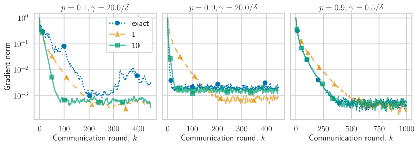
Figure 1: Convergence of SPAM-inexact on a ridge regression problem with different $p$ and $\gamma$.

7 Conclusion

We introduced SPAM, an algorithm tailored for cross-device federated learning, which combines momentum variance reduction with the stochastic proximal point method. Operating under second-order heterogeneity and bounded variance conditions, SPAM does not necessitate smoothness of the objective function. In its most general form, SPAM achieves optimal communication complexity. Furthermore, it does not prescribe a specific local method for analysis, providing practitioners with flexibility and responsibility in selecting suitable local solver.

Limitations and future work.

The paper is of a theoretical nature and focuses on improving the understanding of stochastic non-convex optimization under Hessian similarity in the context of cross-device federated learning. We believe that separate experiments should be conducted to evaluate the experimental performance in a setting close to real life.

In standard optimization, the stepsize usually depends on the smoothness parameter. Adaptive methods allow iterative adjustment of the stepsize without additional information. In our case, the smoothness parameter is replaced by the second-order heterogeneity parameter $\delta$, on which the stepsize and momentum sequences of SPAM depend. Removing this dependence using adaptive techniques under general assumptions remains an open problem even for the server-only MVR, which serves as the basis for our algorithm.

Finally, federated learning comprises other aspects that we have not discussed above. These include privacy, security, personalization, etc., while our focus is on optimization and communication complexity. The study of their interplay is vital in future work. Our flexible framework can be beneficial due to the significantly simpler theory in contrast to prior works KJK⁺ (21); PWW⁺ (22).

Appendix A Convergence analysis for SPAM

A.1 Proof of Proposition 3.1

Recall that

$$V_{k}=f(x_{k})-f_{\inf}+\frac{3\gamma_{k}}{2p_{k}-p_{k}^{2}}{\left\|g_{k}-\nabla f(x_{k})\right\|^{2}}.$$

We bound each term separately. We formulate three technical lemmas that are inspired by [26]. Their proofs can be found in Appendix E. We start by bounding the first term of the Lyapunov function, which is the function values.

Lemma A.1.

Under the conditions of Proposition 3.1, the following recurrent inequality takes place

$$f(x_{k+1})-f_{\inf}\leq f(x_{k})-f_{\inf}-\frac{1}{4\gamma_{k}}{\left\|x_{k+1}-x_{k}\right\|^{2}}+2\gamma_{k}{\left\|\nabla f(x_{k})-g_{k}\right\|^{2}}$$ (12)

Then, we bound the second term of $V_{k}$.

Lemma A.2.

Under the conditions of Proposition 3.1, the following recurrent inequality takes place

$${\rm E}\left[\left.{\left\|g_{k+1}-\nabla f(x_{k+1})\right\|^{2}}\right|\mathcal{F}_{k}\right]\leq(1-p_{k})^{2}{\left\|g_{k}-\nabla f(x_{k})\right\|^{2}}+2(1-p_{k})^{2}\delta^{2}{\left\|x_{k+1}-x_{k}\right\|^{2}}+2p_{k}^{2}\sigma^{2}.$$ (13)

We observe that the term ${\left\|x_{k+1}-x_{k}\right\|^{2}}$ is in both upper bounds. The following lemma provides a lower bound for this expression.

Lemma A.3.

Under the conditions of Proposition 3.1, the following recurrent inequality is true

$${\rm E}\left[{\left\|x_{k+1}-x_{k}\right\|^{2}}\right]\geq\frac{\gamma_{k}^{2}}{4}{\rm E}\left[{\left\|\nabla f(x_{k+1})\right\|^{2}}\right]-\gamma_{k}^{2}{\rm E}\left[{\left\|g_{k}-\nabla f(x_{k})\right\|^{2}}\right].$$ (14)

We now combine the results of the lemmas to bound $V_{K+1}$:

$${\rm E}\left[V_{k+1}\right] \overset{\eqref{eq:step_2}+\eqref{eq:step_1}}{\leq} \alpha(1-p_{k})^{2}{\left\|g_{k}-\nabla f(x_{k})\right\|^{2}}+2\alpha\delta^{2}(1-p_{k})^{2}{\left\|x_{k+1}-x_{k}\right\|^{2}}+2\alpha p_{k}^{2}\sigma^{2}$$

$$+{\rm E}\left[f(x_{k})-f_{\inf}\right]-\frac{1}{4\gamma_{k}}{\rm E}\left[{\left\|x_{k+1}-x_{k}\right\|^{2}}\right]+2\gamma_{k}{\rm E}\left[{\left\|\nabla f(x_{k})-g_{k}\right\|^{2}}\right]$$

$$= {\rm E}\left[V_{k}\right]+\left(2\alpha\delta^{2}(1-p_{k})^{2}-\frac{1}{4\gamma_{k}}\right){\rm E}\left[{\left\|x_{k+1}-x_{k}\right\|^{2}}\right]+2\alpha p_{k}^{2}\sigma^{2}$$

$$+(2\gamma_{k}-\alpha(2p_{k}-p_{k}^{2})){\rm E}\left[{\left\|\nabla f(x_{k})-g_{k}\right\|^{2}}\right].$$

The last inequality is true for every positive value of $\alpha$. Let us now choose $\alpha=\frac{3\gamma_{k}}{2p_{k}-p_{k}^{2}}$. Then,

$$2\alpha\delta^{2}(1-p_{k})^{2}-\frac{1}{4\gamma_{k}}=\frac{6\gamma_{k}\delta^{2}(1-p_{k})^{2}}{2p_{k}-p_{k}^{2}}-\frac{1}{4\gamma_{k}}\leq-\frac{1}{8\gamma_{k}},$$

where the latter is due to $4\delta\gamma_{k}\leq\sqrt{\nicefrac{{p_{k}}}{{6(1-p_{k})}}}$. Therefore, we deduce

$${\rm E}\left[V_{k+1}\right] {\leq} {\rm E}\left[V_{k}\right]-\frac{1}{8\gamma_{k}}{\rm E}\left[{\left\|x_{k+1}-x_{k}\right\|^{2}}\right]-\gamma_{k}{\rm E}\left[{\left\|\nabla f(x_{k})-g_{k}\right\|^{2}}\right]+2\alpha p_{k}^{2}\sigma^{2}$$

$$\overset{\eqref{eq:step_3}}{\leq} {\rm E}\left[V_{k}\right]-\frac{\gamma_{k}}{32}{\rm E}\left[{\left\|\nabla f(x_{k+1})\right\|^{2}}\right]+\frac{\gamma_{k}}{8}{\rm E}\left[{\left\|\nabla f(x_{k})-g_{k}\right\|^{2}}\right]$$

$$-\gamma_{k}{\rm E}\left[{\left\|\nabla f(x_{k})-g_{k}\right\|^{2}}\right]+\frac{6\gamma_{k}p_{k}}{2-p_{k}}\sigma^{2}$$

$$\leq {\rm E}\left[V_{k}\right]-\frac{\gamma_{k}}{32}{\rm E}\left[{\left\|\nabla f(x_{k+1})\right\|^{2}}\right]+6\gamma_{k}p_{k}\sigma^{2}.$$

This concludes the proof of the proposition.

A.2 Proof of Theorem 3.2

Let us apply Proposition 3.1 for the fixed stepsize $\gamma_{k}=\gamma$ and a fixed momentum coefficient $p_{k}=p$.

$${\rm E}\left[V_{k+1}\right] \leq {\rm E}\left[V_{k}\right]-\frac{\gamma}{32}{\rm E}\left[{\left\|\nabla f(x_{k+1})\right\|^{2}}\right]+6\gamma p\sigma^{2}.$$

Summing up these inequalities for $k=0,\ldots,K-1$ leads to

$$\frac{1}{K}\sum_{k=1}^{K}{\rm E}\left[{\left\|\nabla f(x_{k})\right\|^{2}}\right] \leq \frac{32}{\gamma K}\left(V_{0}-{\rm E}\left[V_{K}\right]\right)+192p\sigma^{2}$$

$$\leq \frac{32(f(x_{0})-f_{\inf})}{\gamma K}+\frac{30{\left\|g_{0}-\nabla f(x_{0})\right\|^{2}}}{(2p-p^{2})K}+192p\sigma^{2}.$$

where $\gamma^{2}\leq\min\left\{\frac{1}{16\delta^{2}},\frac{4p}{3\delta^{2}(1-p)}\right\}$. This concludes the proof of the theorem.

A.3 Proof of Theorem 3.5

From Proposition 3.1 we have

$$-\frac{\gamma_{k}}{32}{\rm E}\left[{\left\|\nabla f(x_{k+1})\right\|^{2}}\right] \leq {\rm E}\left[V_{k}\right]-{\rm E}\left[V_{k+1}\right]+6\gamma_{k}p_{k}\sigma^{2}.$$

Let us sum up these inequalities for $k=0,1,\ldots,K-1$. We have a telescoping sum on the right-hand side. Then, dividing both sides on $\Gamma_{K}=\sum_{i=1}^{K}\gamma_{i}$, we deduce the following bound:

$$\frac{1}{\Gamma_{K}}\sum_{k=1}^{K}\gamma_{k}{\rm E}\left[{\left\|\nabla f(x_{k})\right\|^{2}}\right]\leq\frac{32V_{0}}{\Gamma_{K}}+\frac{2}{\Gamma_{K}}\sum_{k=1}^{K}\frac{15\delta^{2}\gamma_{k}^{3}}{15\delta^{2}\gamma_{k}^{2}+4}\sigma^{2}.$$

This concludes the proof.

A.4 Proof of Theorem 4.1

We start by repeating the steps of the proof for Proposition 3.1. Notice that the proposition statement assumes that the iterate is exactly equal to the proximal point operator. However, as stated in Section 4, in the proofs of lemmas A.1 and A.2 we only use the property that $\phi_{k}(x_{k+1})\leq\phi_{k}(x_{k})$ (see (21)). Thus, both (12) and (13) are true for SPAM-inexact. Therefore,

$${\rm E}\left[V_{k+1}\right] {\leq}\quad{\rm E}\left[V_{k}\right] -\frac{1}{8\gamma_{k}}{\rm E}\left[{\left\|x_{k+1}-x_{k}\right\|^{2}}\right]-(2\gamma_{k}-\alpha(2p_{k}-p_{k}^{2})){\rm E}\left[{\left\|\nabla f(x_{k})-g_{k}\right\|^{2}}\right]$$

$$+2\alpha p_{k}^{2}\sigma^{2}.$$

Below, reformulate the adaptation of Lemma A.3 for the inexact case to lower bound the second term on the right-hand side.

Lemma A.4.

Under the conditions of Proposition 3.1, we have the following bound

$${\rm E}\left[{\left\|x_{k+1}-x_{k}\right\|^{2}}\right]\geq\frac{\gamma_{k}^{2}}{5}{\rm E}\left[{\left\|\nabla f(x_{k+1})\right\|^{2}}\right]-\gamma_{k}^{2}{\rm E}\left[{\left\|g_{k}-\nabla f(x_{k})\right\|^{2}}\right]-\gamma_{k}^{2}\epsilon^{2}.$$ (15)

The proof can be found in Section E.4. Thus,

$${\rm E}\left[V_{k+1}\right] \overset{\eqref{eq:step3_inexact}}{\leq} {\rm E}\left[V_{k}\right]-\frac{\gamma_{k}}{40}{\rm E}\left[{\left\|\nabla f(x_{k+1})\right\|^{2}}\right]+\frac{15\gamma_{k}p_{k}}{8(2-p_{k})}\sigma^{2}+\frac{\gamma_{k}\epsilon^{2}}{8}$$

$$+\frac{\gamma_{k}}{8}{\rm E}\left[{\left\|\nabla f(x_{k})-g_{k}\right\|^{2}}\right]-(2\gamma_{k}-\alpha(2p_{k}-p_{k}^{2})){\rm E}\left[{\left\|\nabla f(x_{k})-g_{k}\right\|^{2}}\right]$$

$$\leq {\rm E}\left[V_{k}\right]-\frac{\gamma_{k}}{40}{\rm E}\left[{\left\|\nabla f(x_{k+1})\right\|^{2}}\right]+2\gamma_{k}p_{k}\sigma^{2}+\frac{\gamma_{k}\epsilon^{2}}{8}.$$

Repeating this step for $k=0,\ldots,K-1$, we deduce

$$\frac{1}{\Gamma_{K}}\sum_{k=0}^{K-1}\gamma_{k}{\rm E}\left[{\left\|\nabla f(x_{k+1})\right\|^{2}}\right] \leq \frac{40V_{0}}{\Gamma_{K}}+\frac{2}{\Gamma_{K}}\sum_{k=0}^{K-1}\frac{15\sigma^{2}\gamma_{k}^{3}}{15\sigma^{2}\gamma_{k}^{2}+4}\sigma^{2}+\frac{\epsilon^{2}}{8}.$$

Appendix B Proof of Theorem 5.1

The proof follows the logic of Proposition 3.1. Recall that

$$V_{k}=f(x_{k})-f_{\inf}+\frac{3\gamma_{k}}{2p_{k}-p_{k}^{2}}{\left\|g_{k}-\nabla f(x_{k})\right\|^{2}}.$$

Recall that Lemma A.1 is true for any gradient estimator $g_{k}$. Thus, (12) is also valid for SPAM-PP. Next, we estimate the second term of the Lyapunov function. Recall that

$$g_{k+1} =\frac{1}{S_{k}}\sum_{i\in S_{k}}\left\{\nabla f_{i}(x_{k+1})+(1-p_{k})\left(g_{k}-\nabla f_{i}(x_{k})\right)\right\}$$

$$=\nabla\tilde{f}_{k}(x_{k+1})+(1-p_{k})\left(g_{k}-\nabla\tilde{f}_{k}(x_{k})\right),$$

where $\tilde{f}_{k}(x):=\frac{1}{S_{k}}\sum_{i\in S_{k}}\nabla f_{i}(x)$. Notice also that ${\rm E}\left[\tilde{f}_{k}(x)\right]=f(x)$, for every fixed $x\in\mathbb{R}^{d}$. Furthermore, combining the convexity of the Euclidean norm and Hessian similarity (5) we deduce that the estimator $\tilde{f}_{k}$ satisfies the Hessian similarity condition

$${\left\|\nabla\tilde{f}_{k}(x)-\nabla f(x)-\nabla\tilde{f}_{k}(y)+\nabla f(y)\right\|} \leq\frac{1}{B}\sum_{i\in S_{k}}{\left\|\nabla{f}_{i}(x)-\nabla f(x)-\nabla{f}_{i}(y)+\nabla f(y)\right\|}$$

$$\leq\frac{\delta}{B}{\left\|x-y\right\|}.$$

Finally, Jensen’s inequality implies that $\tilde{f}_{k}$ satisfies the bounded variance condition as well:

$${\rm E}\left[{\left\|\nabla\tilde{f}_{k}(x)-\nabla f(x)\right\|}\right]\leq\sigma^{2}/B.$$

Repeating the analysis exactly as in the proof of Lemma A.2, we obtain

$${\rm E}\left[{\left\|g_{k+1}-\nabla f(x_{k+1})\right\|^{2}}\right] \leq (1-p_{k})^{2}{\rm E}\left[{\left\|g_{k}-\nabla f(x_{k})\right\|^{2}}\right]$$ (16)

$$+2(1-p_{k})^{2}\frac{\delta^{2}}{B^{2}}{\rm E}\left[{\left\|x_{k+1}-x_{k}\right\|^{2}}\right]+\frac{2p_{k}^{2}\sigma^{2}}{B}.$$

Let us now bound the Lyapunov function using (12) and (16):

$${\rm E}\left[V_{k+1}\right] {\leq} {\rm E}\left[f(x_{k})-f_{\inf}\right]+{2\gamma_{k}}{\rm E}\left[{\left\|\nabla f(x_{k})-g_{k}\right\|^{2}}\right]-\frac{1}{4\gamma_{k}}{\rm E}\left[{\left\|x_{k+1}-x_{k}\right\|^{2}}\right]$$

$$+\alpha(1-p_{k})^{2}{\rm E}\left[{\left\|g_{k}-\nabla f(x_{k})\right\|^{2}}\right]+2\alpha(1-p_{k})^{2}\frac{\delta^{2}}{B^{2}}{\rm E}\left[{\left\|x_{k+1}-x_{k}\right\|^{2}}\right]+\frac{2\alpha p_{k}^{2}\sigma^{2}}{B}$$

$$= {\rm E}\left[V_{k}\right]+\left(2\alpha\frac{\delta^{2}}{B^{2}}(1-p_{k})^{2}-\frac{1}{4\gamma_{k}}\right){\rm E}\left[{\left\|x_{k+1}-x_{k}\right\|^{2}}\right]+\frac{2\alpha p_{k}^{2}\sigma^{2}}{B}$$

$$+(2\gamma_{k}-\alpha(2p_{k}-p_{k}^{2})){\rm E}\left[{\left\|\nabla f(x_{k})-g_{k}\right\|^{2}}\right].$$

The latter is true for every positive $\alpha$. Let us now plug in the value of $\alpha=\frac{3\gamma_{k}}{2p_{k}-p_{k}^{2}}$. Then, using $\gamma\leq\sqrt{\frac{B^{2}p_{k}}{96\delta^{2}(1-p_{k})}}$, we obtain

$$2\alpha\frac{\delta^{2}}{B^{2}}(1-p_{k})^{2}-\frac{1}{4\gamma_{k}}\leq\frac{6\gamma_{k}\delta^{2}}{B^{2}(2p_{k}-p_{k}^{2})}(1-p_{k})^{2}-\frac{1}{4\gamma_{k}}\leq-\frac{1}{8\gamma_{k}}.$$ (17)

Hence, we have the following bound

$${\rm E}\left[V_{k+1}\right] {\leq} {\rm E}\left[V_{k}\right]-\frac{1}{8\gamma_{k}}{\rm E}\left[{\left\|x_{k+1}-x_{k}\right\|^{2}}\right]-\gamma_{k}{\rm E}\left[{\left\|\nabla f(x_{k})-g_{k}\right\|^{2}}\right]+\frac{6p_{k}\gamma_{k}\sigma^{2}}{B(2-p_{k})}$$

$$\overset{\eqref{eq:step3_inexact}}{\leq} {\rm E}\left[V_{k}\right]-\frac{1}{8\gamma_{k}}\left(\frac{\gamma_{k}^{2}}{5}{\rm E}\left[{\left\|\nabla f(x_{k+1})\right\|^{2}}\right]-\gamma_{k}^{2}{\rm E}\left[{\left\|g_{k}-\nabla f(x_{k})\right\|^{2}}\right]-\gamma_{k}^{2}\epsilon^{2}\right)$$

$$-\gamma_{k}{\rm E}\left[{\left\|\nabla f(x_{k})-g_{k}\right\|^{2}}\right]+\frac{6p_{k}\gamma_{k}\sigma^{2}}{B}$$

$${\leq} {\rm E}\left[V_{k}\right]-\frac{\gamma_{k}}{40}{\rm E}\left[{\left\|\nabla f(x_{k+1})\right\|^{2}}\right]-\frac{7\gamma_{k}}{8}{\rm E}\left[{\left\|\nabla f(x_{k})-g_{k}\right\|^{2}}\right]+\frac{6p_{k}\gamma_{k}\sigma^{2}}{B}+\frac{\gamma_{k}\epsilon^{2}}{8}$$

$$\leq {\rm E}\left[V_{k}\right]-\frac{\gamma_{k}}{40}{\rm E}\left[{\left\|\nabla f(x_{k+1})\right\|^{2}}\right]+\frac{6p_{k}\gamma_{k}\sigma^{2}}{B}+\frac{\gamma_{k}\epsilon^{2}}{8}.$$

Thus, we have

$$\frac{1}{\Gamma_{K}}\sum_{k=0}^{K-1}\gamma_{k}{\rm E}\left[{\left\|\nabla f(x_{k+1})\right\|^{2}}\right] \leq \frac{40}{\Gamma_{K}}\left(V_{0}-{\rm E}\left[V_{K}\right]\right)+\frac{240}{\Gamma_{K}}\sum_{k=0}^{K-1}p_{k}\gamma_{k}\frac{\sigma^{2}}{B}+{7.5\epsilon^{2}}.$$

This concludes the proof of the theorem.

Appendix C Complexity analysis of the methods

We use $\lesssim$ to ignore numerical constants in the subsequent analysis.

C.1 Proof of Corollary 3.4

We have stepsize condition $\gamma\lesssim\min\{1/\delta,\sqrt{p/(\delta^{2}(1-p))}\}$, which implies that $\gamma\lesssim\sqrt{p}/\delta$ or $p\gtrsim(\gamma\delta)^{2}$. Denote $F:=f(x_{0})-f_{\inf}$, then convergence rate of SPAM can be expressed as

$$R_{K}:=\frac{1}{K}\sum_{k=1}^{K}{\rm E}\left[{\left\|\nabla f(x_{k})\right\|^{2}}\right] \lesssim \frac{f(x_{0})-f_{\inf}}{\gamma K}+\frac{{\left\|g_{0}-\nabla f(x_{0})\right\|^{2}}}{(2p-p^{2})K}+p\sigma^{2}$$

$$\lesssim \frac{F}{\gamma K}+\frac{{\left\|g_{0}-\nabla f(x_{0})\right\|^{2}}}{pK}+p\sigma^{2},$$

where in the last inequality, we used condition for the stepsize and the fact that $p(2-p)\geq p$. Next, by using an argument similar to that in [14], we suppose (without loss of generality) that the method is run for $K$ iterations. For the first $K/2$ iterations, we simply sample $\nabla f_{\xi}$ at $x_{0}$ to set $g_{0}=\frac{1}{K/2}\sum_{i=1}^{K/2}\nabla f_{\xi_{i}}(x_{0})$. Then, according to (3), we have ${\rm E}\left[{\left\|g_{0}-\nabla f(x_{0})\right\|^{2}}\right]\leq\frac{\sigma^{2}}{K/2}.$ Now, choose $p=\max(\gamma^{2}\delta^{2},1/K)$

$$R_{K}\lesssim\frac{F}{\gamma K}+\frac{\sigma^{2}}{pK^{2}}+p\sigma^{2}\lesssim\frac{F}{\gamma K}+\frac{\sigma^{2}}{K}+\gamma^{2}\delta^{2}\sigma^{2}+\frac{\sigma^{2}}{K}.$$

Next set $\gamma=\min\left(\frac{1}{\delta},\left(\frac{F}{2\delta^{2}\sigma^{2}K}\right)^{1/3}\right)$ and the rate results in

$$R_{K} \lesssim \frac{\delta F}{K}+\frac{F}{K}\left(\frac{2\delta^{2}\sigma^{2}K}{F}\right)^{1/3}+\left(\frac{F}{2\delta^{2}\sigma^{2}K}\right)^{2/3}\delta^{2}\sigma^{2}+\frac{\sigma^{2}}{K}$$

$$\lesssim \frac{\delta F+\sigma^{2}}{K}+\left(\frac{\delta\sigma F}{K}\right)^{2/3},$$

which leads to the communication complexity of $\mathcal{O}\left(\frac{\delta F+\sigma^{2}}{\varepsilon}+\frac{\delta\sigma F}{\varepsilon^{3/2}}\right)$. This concludes the proof.

C.2 Proof of Corollary 5.2

In this part, we analyze communication complexity similar to Section C.2. The focus is on constant stepsize case $\gamma_{k}\equiv\gamma\lesssim\min\{1/\delta,\sqrt{p}B/\delta\}$ and exact proximal computation $\epsilon=0$. Denote $F:=f(x_{0})-f_{\inf}$, then convergence rate of SPAM-PP can be expressed as

$$R_{K}:=\frac{1}{K}\sum_{k=1}^{K}{\rm E}\left[{\left\|\nabla f(x_{k})\right\|^{2}}\right] \lesssim \frac{F}{\gamma K}+\frac{{\left\|g_{0}-\nabla f(x_{0})\right\|^{2}}}{pK}+\frac{p\sigma^{2}}{B}.$$

By using the same reasoning as in C.1 set

$$g_{0}=\frac{1}{BK/2}\sum_{j=1}^{K/2}\sum_{i=1}^{S_{j}}\nabla f_{\xi_{i}}(x_{0})$$

to make sure ${\rm E}\left[{\left\|g_{0}-\nabla f(x_{0})\right\|^{2}}\right]\leq\sigma^{2}/(BK/2)$. Then

$$R_{K}\lesssim\frac{F}{\gamma K}+\frac{\sigma^{2}}{pBK^{2}}+\frac{p\sigma^{2}}{B}.$$

Now choose $p=\max(\gamma^{2}\delta^{2},1/K)$ which leads to

$$R_{K}\lesssim\frac{F}{\gamma K}+\frac{\sigma^{2}}{BK}+\frac{\gamma^{2}\delta^{2}\sigma^{2}}{B}+\frac{\sigma^{2}}{BK}.$$

Next set $\gamma=\min\left(\frac{1}{\delta},\left(\frac{BF}{2\delta^{2}\sigma^{2}K}\right)^{1/3}\right)$ and the rate results in

$$R_{K} \lesssim \frac{\delta F}{K}+\frac{F}{K}\left(\frac{2\delta^{2}\sigma^{2}K}{BF}\right)^{1/3}+\frac{\sigma^{2}}{BK}+\left(\frac{BF}{2\delta^{2}\sigma^{2}K}\right)^{2/3}\frac{\delta^{2}\sigma^{2}}{B}+\frac{\sigma^{2}}{BK}$$

$$\lesssim \frac{\delta F}{K}+\frac{\sigma^{2}}{BK}+\left(\frac{\delta\sigma F}{\sqrt{B}K}\right)^{2/3},$$

which leads to communication complexity

$$\mathcal{O}\left(\frac{\delta F}{\varepsilon}+\frac{\sigma^{2}}{B\varepsilon}+\frac{\delta\sigma F}{\sqrt{B}\varepsilon^{3/2}}\right).$$

Appendix D Partial participation with averaging

1:  Input: learning rate $\gamma>0$, starting point $x_{0}\in\mathbb{R}^{d}$; proximal precision level $\epsilon$; initialize $g_{0}=g_{-1}$;

2:  for $k=0,1,2,\ldots$ do

3:     Sample a subset of clients $S_{k}$, with size $|S_{k}|=B$;

4:     Selected clients do local SPAM updates;

5:     for $i\in S_{k}$ do

6:        Set $g_{k}^{i}=\nabla f_{i}(x_{k})+(1-p_{k})\left(g_{k-1}-\nabla f_{i}(x_{k-1})\right)$;

7:        Broadcast $g_{k}^{i}$ to the server;

8:     end for

9:     $g_{k}=\frac{1}{B}\sum_{i\in S_{k}}g_{k}^{i}$ ;

10:     for $i\in S_{k}$ do

11:        Set $x_{k+1}^{i}={\rm a\text{-}prox}_{\epsilon}\left(x_{k},g_{k},\gamma_{k},i\right)$;

12:        Broadcast $x_{k+1}^{i}$ to the server;

13:     end for

14:     The server aggregates the local iterates: $x_{k+1}=\frac{1}{B}\sum_{i\in S_{k}}x_{k+1}^{i}$;

15:  end for

Algorithm 3 SPAM-PPA

Theorem D.1 (SPAM-PPA).

Suppose Assumptions 1, 2 are satisfied and the objective function $f$ is $L$-smooth. If $\xi_{k}\sim{\sf Unif}(S_{k})$ at every iteration, then the iterates of SPAM-PPA with $\gamma_{k}\leq\frac{1}{4(\delta+L)}$ and $p_{k}=\frac{96\delta^{2}\gamma_{k}^{2}}{96\delta^{2}\gamma_{k}^{2}+B^{2}}$ satisfy

$$\frac{1}{\Gamma_{K}}\sum_{k=0}^{K-1}\gamma_{k}{\rm E}\left[{\left\|\nabla f(x^{\xi}_{k+1})\right\|^{2}}\right] \leq \frac{40}{\Gamma_{K}}\left(V_{0}-{\rm E}\left[V_{K}\right]\right)+\frac{240}{\Gamma_{K}}\sum_{k=0}^{K-1}p_{k}\gamma_{k}\frac{\sigma^{2}}{B}+{7.5\epsilon^{2}}.$$

The result of the theorem is similar to the one in Theorem 5.1. In fact, following the proof scheme of Corollary 5.2, one can derive the complexity analysis for SPAM-PPA. However, unlike previous results, we require the objective function $f$ to be smooth.

D.1 Proof of Theorem D.1

The proof follows the logic of Proposition 3.1. Recall that

$$V_{k}=f(x_{k})-f_{\inf}+\frac{3\gamma_{k}}{2p_{k}-p_{k}^{2}}{\left\|g_{k}-\nabla f(x_{k})\right\|^{2}}.$$

We start with proving a descent lemma. Recall that $\xi_{k}\sim{\sf Unif}(S_{k})$, for the fixed $S_{k}$.

Lemma D.2.

For an $L$-smooth objective $f$ satisfying assumptions 1,2 and parameters $\gamma_{k}^{2}\leq\min\left\{\frac{1}{16(L+\delta)^{2}},\frac{4p_{k}}{15\delta^{2}(1-p_{k})}\right\}$, the iterates of the SPAM-PPA algorithm satisfy

$${\rm E}\left[f(x_{k+1})-f_{\inf}\right]\leq{\rm E}\left[f(x_{k})-f_{\inf}\right]+{2\gamma_{k}}{\rm E}\left[{\left\|\nabla f(x_{k})-g_{k}\right\|^{2}}\right]-\frac{1}{4\gamma_{k}}{\rm E}\left[{\left\|x^{\xi_{k}}_{k+1}-x_{k}\right\|^{2}}\right].$$ (18)

The proof of the lemma is deferred to Section E.5. Next, we estimate the second term of the Lyapunov function. Recall that

$$g_{k+1} =\frac{1}{S_{k}}\sum_{i\in S_{k}}\left\{\nabla f_{i}(x_{k+1})+(1-p_{k})\left(g_{k}-\nabla f_{i}(x_{k})\right)\right\}$$

$$=\nabla\tilde{f}_{k}(x_{k+1})+(1-p_{k})\left(g_{k}-\nabla\tilde{f}_{k}(x_{k})\right),$$

where $\tilde{f}_{k}(x):=\frac{1}{S_{k}}\sum_{i\in S_{k}}\nabla f_{i}(x)$. Notice that ${\rm E}\left[\tilde{f}_{k}(x)\right]=f(x)$, for every fixed $x\in\mathbb{R}^{d}$. Furthermore, combining the convexity of the Euclidean norm and Hessian similarity (5) we deduce that the estimator $\tilde{f}_{k}$ satisfies the Hessian similarity condition

$${\left\|\nabla\tilde{f}_{k}(x)-\nabla f(x)-\nabla\tilde{f}_{k}(y)+\nabla f(y)\right\|} \leq\frac{1}{B}\sum_{i\in S_{k}}{\left\|\nabla{f}_{i}(x)-\nabla f(x)-\nabla{f}_{i}(y)+\nabla f(y)\right\|}$$

$$\leq\frac{\delta}{B}{\left\|x-y\right\|}.$$

Furthermore, Jensen’s inequality implies that $\tilde{f}_{k}$ satisfies the bounded variance condition as well:

$${\rm E}\left[{\left\|\nabla\tilde{f}_{k}(x)-\nabla f(x)\right\|}\right]\leq\sigma^{2}/B.$$

Repeating the analysis exactly as in the proof of Lemma A.2, we obtain

$${\rm E}\left[{\left\|g_{k+1}-\nabla f(x_{k+1})\right\|^{2}}\right] \leq (1-p_{k})^{2}{\rm E}\left[{\left\|g_{k}-\nabla f(x_{k})\right\|^{2}}\right]$$

$$+2(1-p_{k})^{2}\frac{\delta^{2}}{B^{2}}{\rm E}\left[{\left\|x_{k+1}-x_{k}\right\|^{2}}\right]+\frac{2p_{k}^{2}\sigma^{2}}{B}.$$

Assume now that $\xi_{k}\sim{\sf Unif}(S_{k})$, for a fixed $S_{k}$. The latter means $x_{k+1}={\rm E}\left[\left.x^{\xi_{k}}_{k+1}\right|\mathcal{G}_{k}\right]$, and subsequently, Jensen’s inequality yields

$${\rm E}\left[{\left\|g_{k+1}-\nabla f(x_{k+1})\right\|^{2}}\right]{\leq} (1-p_{k})^{2}{\rm E}\left[{\left\|g_{k}-\nabla f(x_{k})\right\|^{2}}\right]$$

$$+2(1-p_{k})^{2}\frac{\delta^{2}}{B^{2}}{\rm E}\left[{\left\|{\rm E}\left[\left.x^{\xi_{k}}_{k+1}\right|\mathcal{G}_{k}\right]-x_{k}\right\|^{2}}\right]+\frac{2p_{k}^{2}\sigma^{2}}{B}$$

$${\leq} (1-p_{k})^{2}{\rm E}\left[{\left\|g_{k}-\nabla f(x_{k})\right\|^{2}}\right]$$

$$+2(1-p_{k})^{2}\frac{\delta^{2}}{B^{2}}{\rm E}\left[{\rm E}\left[\left.{\left\|x^{\xi_{k}}_{k+1}-x_{k}\right\|^{2}}\right|\mathcal{G}_{k}\right]\right]+\frac{2p_{k}^{2}\sigma^{2}}{B}$$

$$= (1-p_{k})^{2}{\rm E}\left[{\left\|g_{k}-\nabla f(x_{k})\right\|^{2}}\right]$$

$$+2(1-p_{k})^{2}\frac{\delta^{2}}{B^{2}}{\rm E}\left[{\left\|x^{\xi_{k}}_{k+1}-x_{k}\right\|^{2}}\right]+\frac{2p_{k}^{2}\sigma^{2}}{B}.$$

Now, we need to bound ${\rm E}\left[{\left\|x^{\xi_{k}}_{k+1}-x_{k}\right\|^{2}}\right]$ from below.

Lemma D.3.

Under assumptions 1 and 2, we have the following lower bound for the iterates of SPAM-PPA algorithm

$${\rm E}\left[{\left\|x^{\xi_{k}}_{k+1}-x_{k}\right\|^{2}}\right]\geq\frac{\gamma_{k}^{2}}{5}{\rm E}\left[{\left\|\nabla f(x^{\xi_{k}}_{k+1})\right\|^{2}}\right]-\gamma_{k}^{2}{\rm E}\left[{\left\|g_{k}-\nabla f(x_{k})\right\|^{2}}\right]-\gamma_{k}\epsilon^{2}.$$ (19)

The proof of the lemma can be found in Section E.6. Let us now bound the Lyapunov function using (18) and (D.1):

$${\rm E}\left[V_{k+1}\right] {\leq} {\rm E}\left[f(x_{k})-f_{\inf}\right]+{2\gamma_{k}}{\rm E}\left[{\left\|\nabla f(x_{k})-g_{k}\right\|^{2}}\right]-\frac{1}{4\gamma_{k}}{\rm E}\left[{\left\|x^{\xi_{k}}_{k+1}-x_{k}\right\|^{2}}\right]$$

$$+\alpha(1-p_{k})^{2}{\rm E}\left[{\left\|g_{k}-\nabla f(x_{k})\right\|^{2}}\right]+2\alpha(1-p_{k})^{2}\frac{\delta^{2}}{B^{2}}{\rm E}\left[{\left\|x^{\xi_{k}}_{k+1}-x_{k}\right\|^{2}}\right]+\frac{2\alpha p_{k}^{2}\sigma^{2}}{B}$$

$$= {\rm E}\left[V_{k}\right]+\left(2\alpha\frac{\delta^{2}}{B^{2}}(1-p_{k})^{2}-\frac{1}{4\gamma_{k}}\right){\rm E}\left[{\left\|x^{\xi_{k}}_{k+1}-x_{k}\right\|^{2}}\right]+\frac{2\alpha p_{k}^{2}\sigma^{2}}{B}$$

$$+(2\gamma_{k}-\alpha(2p_{k}-p_{k}^{2})){\rm E}\left[{\left\|\nabla f(x_{k})-g_{k}\right\|^{2}}\right].$$

The latter is true for every positive $\alpha$. Let us now plug in the value of $\alpha=\frac{3\gamma_{k}}{2p_{k}-p_{k}^{2}}$. Then, using $\gamma\leq\sqrt{\frac{B^{2}p_{k}}{96\delta^{2}(1-p_{k})}}$, we obtain

$$2\alpha\frac{\delta^{2}}{B^{2}}(1-p_{k})^{2}-\frac{1}{4\gamma_{k}}\leq\frac{6\gamma_{k}\delta^{2}}{B^{2}(2p_{k}-p_{k}^{2})}(1-p_{k})^{2}-\frac{1}{4\gamma_{k}}\leq-\frac{1}{8\gamma_{k}}.$$ (20)

Hence, we have the following bound

$${\rm E}\left[V_{k+1}\right] {\leq} {\rm E}\left[V_{k}\right]-\frac{1}{8\gamma_{k}}{\rm E}\left[{\left\|x^{\xi_{k}}_{k+1}-x_{k}\right\|^{2}}\right]-\gamma_{k}{\rm E}\left[{\left\|\nabla f(x_{k})-g_{k}\right\|^{2}}\right]+\frac{6p_{k}\gamma_{k}\sigma^{2}}{B(2-p_{k})}$$

$$\overset{\eqref{eq:step_3-pp}}{\leq} {\rm E}\left[V_{k}\right]-\frac{1}{8\gamma_{k}}\left(\frac{\gamma_{k}^{2}}{5}{\rm E}\left[{\left\|\nabla f(x^{\xi_{k}}_{k+1})\right\|^{2}}\right]-\gamma_{k}^{2}{\rm E}\left[{\left\|g_{k}-\nabla f(x_{k})\right\|^{2}}\right]-\gamma_{k}^{2}\epsilon^{2}\right)$$

$$-\gamma_{k}{\rm E}\left[{\left\|\nabla f(x_{k})-g_{k}\right\|^{2}}\right]+\frac{6p_{k}\gamma_{k}\sigma^{2}}{B}$$

$${\leq} {\rm E}\left[V_{k}\right]-\frac{\gamma_{k}}{40}{\rm E}\left[{\left\|\nabla f(x^{\xi_{k}}_{k+1})\right\|^{2}}\right]-\frac{7\gamma_{k}}{8}{\rm E}\left[{\left\|\nabla f(x_{k})-g_{k}\right\|^{2}}\right]+\frac{6p_{k}\gamma_{k}\sigma^{2}}{B}+\frac{\gamma_{k}\epsilon^{2}}{8}$$

$$\leq {\rm E}\left[V_{k}\right]-\frac{\gamma_{k}}{40}{\rm E}\left[{\left\|\nabla f(x^{\xi_{k}}_{k+1})\right\|^{2}}\right]+\frac{6p_{k}\gamma_{k}\sigma^{2}}{B}+\frac{\gamma_{k}\epsilon^{2}}{8}.$$

Thus, we have

$$\frac{1}{\Gamma_{K}}\sum_{k=0}^{K-1}\gamma_{k}{\rm E}\left[{\left\|\nabla f(x^{\xi_{k}}_{k+1})\right\|^{2}}\right] \leq \frac{40}{\Gamma_{K}}\left(V_{0}-{\rm E}\left[V_{K}\right]\right)+\frac{240}{\Gamma_{K}}\sum_{k=0}^{K-1}p_{k}\gamma_{k}\frac{\sigma^{2}}{B}+{7.5\epsilon^{2}}.$$

This concludes the proof of the theorem.

Appendix E Proofs of the technical lemmas

E.1 Proof of Lemma A.1

By the main theorem of Calculus, we have

$$f(x_{k+1})-f(x_{k}) = \int^{1}_{0}\left\langle\nabla f(\underbrace{x_{k}+\tau(x_{k+1}-x_{k})}_{:=x(\tau)}),x_{k+1}-x_{k}\right\rangle d\tau,$$

$$f_{\xi_{k}}(x_{k+1})-f_{\xi_{k}}(x_{k}) = \int^{1}_{0}\left\langle\nabla f_{\xi_{k}}(\underbrace{x_{k}+\tau(x_{k+1}-x_{k})}_{:=x(\tau)}),x_{k+1}-x_{k}\right\rangle d\tau$$

Therefore the difference in function value can be bounded as follows:

$$f(x_{k+1})-f(x_{k}) = f_{\xi_{k}}(x_{k+1})-f_{\xi_{k}}(x_{k})$$

$$+\int^{1}_{0}\left\langle\nabla f(x(\tau))-\nabla f_{\xi_{k}}(x(\tau)),x_{k+1}-x_{k}\right\rangle d\tau$$

$$= f_{\xi_{k}}(x_{k+1})-f_{\xi_{k}}(x_{k})+\left\langle g_{k}-\nabla f_{\xi_{k}}(x_{k}),x_{k+1}-x_{k}\right\rangle$$

$$+\int^{1}_{0}\left\langle\nabla f(x(\tau))-\nabla f_{\xi_{k}}(x(\tau))-g_{k}+\nabla f_{\xi_{k}}(x_{k}),x_{k+1}-x_{k}\right\rangle d\tau$$

$$\leq -\frac{1}{2\gamma_{k}}{\left\|x_{k+1}-x_{k}\right\|^{2}}+\left\langle\nabla f(x_{k})-g_{k},x_{k+1}-x_{k}\right\rangle$$

$$+\int^{1}_{0}\left\langle\nabla f(x(\tau))-\nabla f_{\xi_{k}}(x(\tau))-\nabla f(x_{k})+\nabla f_{\xi_{k}}(x_{k}),x_{k+1}-x_{k}\right\rangle d\tau.$$

The last inequality is due to

$$f_{\xi_{k}}(x_{k+1})+\left\langle g_{k}-\nabla f_{\xi_{k}}(x_{k}),x_{k+1}-x_{k}\right\rangle+\frac{1}{2\gamma_{k}}\|x_{k+1}-x_{k}\|^{2}\leq f_{\xi_{k}}(x_{k}),$$ (21)

which is a direct consequence of $x_{k+1}=\arg\min\limits_{x}\left\{f_{\xi_{k}}(x)+\left\langle g_{k}-\nabla f_{\xi_{k}}(x_{k}),x-x_{k}\right\rangle+\frac{1}{2\gamma_{k}}\|x-x_{k}\|^{2}\right\}$. Let us now apply Cauchy-Schwartz inequality to bound both scalar products:

$$f(x_{k+1})-f(x_{k}) \leq -\frac{1}{2\gamma_{k}}{\left\|x_{k+1}-x_{k}\right\|^{2}}+2\gamma_{k}{\left\|\nabla f(x_{k})-g_{k}\right\|^{2}}+\frac{1}{8\gamma_{k}}{\left\|x_{k+1}-x_{k}\right\|^{2}}$$

$$+\int^{1}_{0}{\left\|\nabla f(x(\tau))-\nabla f_{\xi_{k}}(x(\tau))-\nabla f(x_{k})+\nabla f_{\xi_{k}}(x_{k})\right\|}{\left\|x_{k+1}-x_{k}\right\|}d\tau$$

$$\overset{\eqref{eq:similarity_almost_sure}}{\leq} -\frac{1}{2\gamma_{k}}{\left\|x_{k+1}-x_{k}\right\|^{2}}+2\gamma_{k}{\left\|\nabla f(x_{k})-g_{k}\right\|^{2}}+\frac{1}{8\gamma_{k}}{\left\|x_{k+1}-x_{k}\right\|^{2}}$$

$$+\delta\int^{1}_{0}{\left\|x(\tau)-x_{k}\right\|}{\left\|x_{k+1}-x_{k}\right\|}d\tau$$

$$= -\frac{1}{2\gamma_{k}}{\left\|x_{k+1}-x_{k}\right\|^{2}}+2\gamma_{k}{\left\|\nabla f(x_{k})-g_{k}\right\|^{2}}+\frac{1}{8\gamma_{k}}{\left\|x_{k+1}-x_{k}\right\|^{2}}$$

$$+\frac{\delta}{2}{\left\|x_{k+1}-x_{k}\right\|^{2}}$$

$$\overset{\gamma_{k}\leq\frac{1}{4\delta}}{\leq} -\frac{1}{4\gamma_{k}}{\left\|x_{k+1}-x_{k}\right\|^{2}}+2\gamma_{k}{\left\|\nabla f(x_{k})-g_{k}\right\|^{2}}.$$

Thus, we have

$$f(x_{k+1})-f_{\inf}\leq f(x_{k})-f_{\inf}-\frac{1}{4\gamma_{k}}{\left\|x_{k+1}-x_{k}\right\|^{2}}+2\gamma_{k}{\left\|\nabla f(x_{k})-g_{k}\right\|^{2}}.$$ (22)

This concludes the proof of the lemma.

E.2 Proof of Lemma A.2

Recall that $g_{k+1}=\nabla f_{\xi_{k+1}}(x_{k+1})+(1-p_{k})\left(g_{k}-\nabla f_{\xi_{k+1}}(x_{k})\right)$. We define $\mathcal{F}_{k}:=\{x_{k+1},x_{k},g_{k}\}$. Then,

$${\rm E}\left[\left.{\left\|g_{k+1}-\nabla f(x_{k+1})\right\|^{2}}\right|\mathcal{F}_{k}\right]$$

$$= {\rm E}\left[\left.{\left\|\nabla f_{\xi_{k+1}}(x_{k+1})+(1-p_{k})\left(g_{k}-\nabla f_{\xi_{k+1}}(x_{k})\right)-\nabla f(x_{k+1})\right\|^{2}}\right|\mathcal{F}_{k}\right]$$

$$= {\rm E}\left[\left.{\left\|\nabla f_{\xi_{k+1}}(x_{k+1})-\nabla f(x_{k+1})+(1-p_{k})\left(\nabla f(x_{k})-\nabla f_{\xi_{k+1}}(x_{k})\right)\right\|^{2}}\right|\mathcal{F}_{k}\right]$$

$$+(1-p_{k})^{2}{\left\|g_{k}-\nabla f(x_{k})\right\|^{2}}.$$

The last equality is due to the bias-variance formula and the fact that $\xi_{k+1}$ is independent of $\mathcal{F}_{k}$ and that the stochastic gradients are unbiased. Using the Cauchy-Schwartz inequality, we deduce the following bound for the first term on the right-hand side, where $\alpha>0$ is an arbitrary constant:

$$\mathrm{E} \left[{\left\|\nabla f_{\xi_{k+1}}(x_{k+1})-\nabla f(x_{k+1})+(1-p_{k})\left(\nabla f(x_{k})-\nabla f_{\xi_{k+1}}(x_{k})\right)\right\|^{2}}\mid{\mathcal{F}_{k}}\right]$$

$$\quad=\mathrm{E}\left[\|p_{k}\left(\nabla f_{\xi_{k+1}}(x_{k+1})-\nabla f(x_{k+1})\right)\right.$$ (23)

$$\qquad+\left.(1-p_{k})\left(\nabla f_{\xi_{k+1}}(x_{k+1})-\nabla f(x_{k+1})+\nabla f(x_{k})-\nabla f_{\xi_{k+1}}(x_{k})\right)\|^{2}\mid{\mathcal{F}_{k}}\right]$$

$$\quad\leq(1+\alpha)p_{k}^{2}{\rm E}\left[\left.{\left\|\nabla f_{\xi_{k+1}}(x_{k+1})-\nabla f(x_{k+1})\right\|^{2}}\right|\mathcal{F}_{k}\right]$$ (24)

$$\qquad+(1+\alpha^{-1})(1-p_{k})^{2}{\rm E}\left[\left.{\left\|\nabla f_{\xi_{k+1}}(x_{k+1})-\nabla f(x_{k+1})+\nabla f(x_{k})-\nabla f_{\xi_{k+1}}(x_{k})\right\|^{2}}\right|\mathcal{F}_{k}\right].$$

We apply (3) and (5) to bound, respectively, the first term and the second term on the right-hand side of (E.2):

$${\rm E}\left[\left.{\left\|\nabla f_{\xi_{k+1}}(x_{k+1})-\nabla f(x_{k+1})+(1-p_{k})\left(\nabla f(x_{k})-\nabla f_{\xi_{k+1}}(x_{k})\right)\right\|^{2}}\right|\mathcal{F}_{k}\right]$$

$$\qquad\leq (1+\alpha)p_{k}^{2}\sigma^{2}+(1+\alpha^{-1})(1-p_{k})^{2}\delta^{2}{\left\|x_{k+1}-x_{k}\right\|^{2}}.$$

Taking $\alpha=1$, we obtain the following

$${\rm E}\left[\left.{\left\|g_{k+1}-\nabla f(x_{k+1})\right\|^{2}}\right|\mathcal{F}_{k}\right]\leq(1-p_{k})^{2}{\left\|g_{k}-\nabla f(x_{k})\right\|^{2}}+2(1-p_{k})^{2}\delta^{2}{\left\|x_{k+1}-x_{k}\right\|^{2}}+2p_{k}^{2}\sigma^{2}.$$

This concludes the proof of the lemma.

E.3 Proof of Lemma A.3

By the definition of $x_{k+1}$, we have

$${\left\|x_{k+1}-x_{k}\right\|^{2}} = \gamma_{k}^{2}{\left\|\nabla f_{\xi_{k}}(x_{k+1})+g_{k}-\nabla f_{\xi_{k}}(x_{k})\right\|^{2}}$$

$$= \gamma_{k}^{2}{\left\|\nabla f(x_{k+1})+g_{k}-\nabla f(x_{k})+\nabla f_{\xi_{k}}(x_{k+1})-\nabla f(x_{k+1})-\nabla f_{\xi_{k}}(x_{k})+\nabla f(x_{k})\right\|^{2}}$$

$$\geq \frac{\gamma_{k}^{2}}{3}{\left\|\nabla f(x_{k+1})\right\|^{2}}-\gamma_{k}^{2}{\left\|g_{k}-\nabla f(x_{k})\right\|^{2}}$$

$$-\gamma_{k}^{2}{\left\|\nabla f_{\xi_{k}}(x_{k+1})-\nabla f(x_{k+1})-\nabla f_{\xi_{k}}(x_{k})+\nabla f(x_{k})\right\|^{2}}$$

$$\geq \frac{\gamma_{k}^{2}}{3}{\left\|\nabla f(x_{k+1})\right\|^{2}}-\gamma_{k}^{2}{\left\|g_{k}-\nabla f(x_{k})\right\|^{2}}-\gamma_{k}^{2}\delta^{2}{\left\|x_{k+1}-x_{k}\right\|^{2}},$$

where we used a variant of Jensen’s inequality $3(a^{2}+b^{2}+c^{2})\geq(a+b+c)^{2}$, for $a,b,c>0$. Therefore, we have

$${\left\|x_{k+1}-x_{k}\right\|^{2}} \geq \frac{1}{1+\gamma_{k}^{2}\delta^{2}}\left(\frac{\gamma_{k}^{2}}{3}{\left\|\nabla f(x_{k+1})\right\|^{2}}-\gamma_{k}^{2}{\left\|g_{k}-\nabla f(x_{k})\right\|^{2}}\right)$$

$$\geq \frac{16}{17}\left(\frac{\gamma_{k}^{2}}{3}{\left\|\nabla f(x_{k+1})\right\|^{2}}-\gamma_{k}^{2}{\left\|g_{k}-\nabla f(x_{k})\right\|^{2}}\right)$$

$$\geq \frac{\gamma_{k}^{2}}{4}{\left\|\nabla f(x_{k+1})\right\|^{2}}-\gamma_{k}^{2}{\left\|g_{k}-\nabla f(x_{k})\right\|^{2}}.$$

Thus, we have

$${\rm E}\left[{\left\|x_{k+1}-x_{k}\right\|^{2}}\right]\geq\frac{\gamma_{k}^{2}}{4}{\rm E}\left[{\left\|\nabla f(x_{k+1})\right\|^{2}}\right]-\gamma_{k}^{2}{\rm E}\left[{\left\|g_{k}-\nabla f(x_{k})\right\|^{2}}\right].$$

This concludes the proof of the lemma.

E.4 Proof of Lemma A.4

Let $x_{k+1}={\rm a\text{-}prox}_{\epsilon}\left(x_{k},g_{k},\gamma_{k},\xi_{k}\right)$. Then, from the definition of the function $\phi_{k}$ (7), we have

$${\left\|x_{k+1}-x_{k}\right\|^{2}} = \gamma_{k}^{2}{\left\|\nabla f_{\xi_{k}}(x_{k+1})+g_{k}-\nabla f_{\xi_{k}}(x_{k}){-\nabla\phi_{k}(x_{k+1})}\right\|^{2}}$$

$$\geq \gamma_{k}^{2}\left(\frac{1}{{4}}{\left\|\nabla f(x_{k+1})\right\|^{2}}-{\left\|g_{k}-\nabla f(x_{k})\right\|^{2}}-\delta^{2}{\left\|x_{k+1}-x_{k}\right\|^{2}}{-{\left\|\nabla\phi_{k}(x_{k+1})\right\|^{2}}}\right).$$

Since ${\left\|a_{1}+a_{2}+a_{3}+a_{4}\right\|^{2}}\leq 4\left(\left\|a_{1}\right\|^{2}+\left\|a_{2}\right\|^{2}+\left\|a_{3}\right\|^{2}+\left\|a_{4}\right\|^{2}\right)$ for any vectors $a_{i}\in\mathbb{R}^{d}$, which implies $\left\|a_{4}\right\|^{2}\geq\frac{1}{4}\left\|a_{1}+a_{2}+a_{3}+a_{4}\right\|^{2}-$ $\left\|a_{1}\right\|^{2}-\left\|a_{2}\right\|^{2}-\left\|a_{3}\right\|^{2}$ and ${\rm E}\left[{\left\|\nabla\phi_{k}(x_{k+1})\right\|^{2}}\right]\leq\epsilon^{2}$, we deduce

$${\left\|x_{k+1}-x_{k}\right\|^{2}}\geq\frac{\gamma_{k}^{2}}{1+\gamma_{k}^{2}\delta^{2}}\left(\frac{1}{4}{\left\|\nabla f(x_{k+1})\right\|^{2}}-{\left\|g_{k}-\nabla f(x_{k})\right\|^{2}}{-\epsilon}\right).$$

Therefore, we have

$${\left\|x_{k+1}-x_{k}\right\|^{2}} \geq \frac{1}{1+\gamma_{k}^{2}\delta^{2}}\left(\frac{\gamma_{k}^{2}}{4}{\left\|\nabla f(x_{k+1})\right\|^{2}}-\gamma_{k}^{2}{\left\|g_{k}-\nabla f(x_{k})\right\|^{2}}-\gamma_{k}^{2}\epsilon^{2}\right)$$

$$\geq \frac{16}{17}\left(\frac{\gamma_{k}^{2}}{4}{\left\|\nabla f(x_{k+1})\right\|^{2}}-\gamma_{k}^{2}{\left\|g_{k}-\nabla f(x_{k})\right\|^{2}}-\gamma_{k}^{2}\epsilon^{2}\right)$$

$$\geq \frac{\gamma_{k}^{2}}{5}{\left\|\nabla f(x_{k+1})\right\|^{2}}-\gamma_{k}^{2}{\left\|g_{k}-\nabla f(x_{k})\right\|^{2}}-\gamma_{k}^{2}\epsilon^{2}.$$

Taking expectations on both sides leads to

$${\rm E}\left[{\left\|x_{k+1}-x_{k}\right\|^{2}}\right]\geq\frac{\gamma_{k}^{2}}{5}{\rm E}\left[{\left\|\nabla f(x_{k+1})\right\|^{2}}\right]-\gamma_{k}^{2}{\rm E}\left[{\left\|g_{k}-\nabla f(x_{k})\right\|^{2}}\right]-\gamma_{k}^{2}\epsilon^{2}.$$

This concludes the proof of the lemma.

E.5 Proof of Lemma D.2

Recalling that $x^{\xi_{k}}_{k+1}={\rm a\text{-}prox}_{\epsilon}\left(x_{k},g_{k},\gamma_{k},\xi_{k}\right)$, we have

$$f_{\xi_{k}}(x^{\xi_{k}}_{k+1})+\left\langle g_{k}-\nabla f_{\xi_{k}}(x_{k}),x^{\xi_{k}}_{k+1}-x_{k}\right\rangle+\frac{1}{2\gamma_{k}}\|x^{\xi_{k}}_{k+1}-x_{k}\|^{2}\leq f_{\xi_{k}}(x_{k}).$$

Similar to the proof of Proposition 3.1 we start with

$$f(x_{k+1})-f(x_{k}) = \int^{1}_{0}\left\langle\nabla f(\underbrace{x_{k}+\tau(x_{k+1}-x_{k})}_{:=x(\tau)}),x_{k+1}-x_{k}\right\rangle d\tau,$$

$$f_{\xi_{k}}(x^{\xi_{k}}_{k+1})-f_{\xi_{k}}(x_{k}) = \int^{1}_{0}\left\langle\nabla f_{\xi_{k}}(\underbrace{x_{k}+\tau(x^{\xi_{k}}_{k+1}-x_{k})}_{:=x^{\xi_{k}}(\tau)}),x^{\xi_{k}}_{k+1}-x_{k}\right\rangle d\tau.$$

Thus, we have

$$f(x_{k+1})-f(x_{k}) = f_{\xi_{k}}(x^{\xi_{k}}_{k+1})-f_{\xi_{k}}(x_{k})$$

$$+\int^{1}_{0}\left\langle\nabla f(x(\tau)),x_{k+1}-x_{k}\right\rangle d\tau$$

$$+\int^{1}_{0}\left\langle-\nabla f_{\xi_{k}}(x^{\xi_{k}}(\tau)),x^{\xi_{k}}_{k+1}-x_{k}\right\rangle d\tau$$

$$= f_{\xi_{k}}(x^{\xi_{k}}_{k+1})-f_{\xi_{k}}(x_{k})+\left\langle g_{k}-\nabla f_{\xi_{k}}(x_{k}),x^{\xi_{k}}_{k+1}-x_{k}\right\rangle$$

$$+\int^{1}_{0}\left\langle\nabla f(x(\tau)),x_{k+1}-x_{k}\right\rangle d\tau$$

$$+\int^{1}_{0}\left\langle-\nabla f_{\xi_{k}}(x^{\xi_{k}}(\tau))-g_{k}+\nabla f_{\xi_{k}}(x_{k}),x^{\xi_{k}}_{k+1}-x_{k}\right\rangle d\tau.$$

Applying the descent property of a-prox (see Definition 4.1), we deduce the following:

$$f(x_{k+1})-f(x_{k}) \leq -\frac{1}{2\gamma_{k}}{\left\|x^{\xi_{k}}_{k+1}-x_{k}\right\|^{2}}+\left\langle\nabla f(x_{k})-g_{k},x^{\xi_{k}}_{k+1}-x_{k}\right\rangle$$

$$+\int^{1}_{0}\left\langle\nabla f(x(\tau)),x_{k+1}-x_{k}\right\rangle d\tau$$

$$+\int^{1}_{0}\left\langle-\nabla f_{\xi_{k}}(x^{\xi_{k}}(\tau))-\nabla f(x_{k})+\nabla f_{\xi_{k}}(x_{k}),x^{\xi_{k}}_{k+1}-x_{k}\right\rangle d\tau.$$

Let us take expectation from both sides conditioned to $\mathcal{G}_{k}=\left\{x_{k},x_{k+1},S_{k},g_{k}\right\}$. In other words, we take expectation with respect to the random index $\xi_{k}$ chosen uniformly from the already chosen $S_{k}$:

$$f(x_{k+1})-f(x_{k}) \leq {\rm E}\left[-\frac{1}{2\gamma_{k}}{\left\|x^{\xi_{k}}_{k+1}-x_{k}\right\|^{2}}+\left\langle\nabla f(x_{k})-g_{k},x^{\xi_{k}}_{k+1}-x_{k}\right\rangle\mid\mathcal{G}_{k}\right]$$

$$+{\rm E}\left[\int^{1}_{0}\left\langle\nabla f(x(\tau)),x_{k+1}-x_{k}\right\rangle d\tau\mid\mathcal{G}_{k}\right]$$

$$+{\rm E}\left[\left.\int^{1}_{0}\left\langle-\nabla f_{\xi_{k}}(x^{\xi_{k}}(\tau))-\nabla f(x_{k})+\nabla f_{\xi_{k}}(x_{k}),x^{\xi_{k}}_{k+1}-x_{k}\right\rangle d\tau\right|\mathcal{G}_{k}\right]$$

$$= {\rm E}\left[-\frac{1}{2\gamma_{k}}{\left\|x^{\xi_{k}}_{k+1}-x_{k}\right\|^{2}}\mid\mathcal{G}_{k}\right]+\left\langle\nabla f(x_{k})-g_{k},x_{k+1}-x_{k}\right\rangle$$

$$+{\rm E}\left[\int^{1}_{0}\left\langle\nabla f(x(\tau))-\nabla f(x_{k})-\nabla f_{\xi_{k}}(x^{\xi_{k}}(\tau))+\nabla f_{\xi_{k}}(x_{k}),x^{\xi_{k}}_{k+1}-x_{k}\right\rangle d\tau\mid\mathcal{G}_{k}\right].$$

Here the last equality is due to the fact that $\xi_{k}$ is independent of $\mathcal{G}_{k}$ and $x_{k+1}={\rm E}\left[x^{\xi_{k}}_{k+1}\mid\mathcal{G}_{k}\right]$. Therefore, applying the Cauchy-Schwartz inequality

$$f(x_{k+1}) -f(x_{k})\leq{\rm E}\left[-\frac{1}{2\gamma_{k}}{\left\|x^{\xi_{k}}_{k+1}-x_{k}\right\|^{2}}\mid\mathcal{G}_{k}\right]+\left\langle\nabla f(x_{k})-g_{k},x_{k+1}-x_{k}\right\rangle$$

$$\quad+{\rm E}\left[\int^{1}_{0}\left\langle\nabla f(x(\tau))-\nabla f(x^{\xi_{k}}(\tau)),x^{\xi_{k}}_{k+1}-x_{k}\right\rangle d\tau\mid\mathcal{G}_{k}\right]$$

$$\quad+{\rm E}\left[\int^{1}_{0}\left\langle\nabla f(x^{\xi_{k}}(\tau))-\nabla f(x_{k})-\nabla f_{\xi_{k}}(x^{\xi_{k}}(\tau))+\nabla f_{\xi_{k}}(x_{k}),x^{\xi_{k}}_{k+1}-x_{k}\right\rangle d\tau\mid\mathcal{G}_{k}\right]$$

$$\leq{\rm E}\left[-\frac{1}{2\gamma_{k}}{\left\|x^{\xi_{k}}_{k+1}-x_{k}\right\|^{2}}\mid\mathcal{G}_{k}\right]+\left\langle\nabla f(x_{k})-g_{k},x_{k+1}-x_{k}\right\rangle$$

$$\quad+{\rm E}\left[\int^{1}_{0}{\left\|\nabla f(x(\tau))-\nabla f(x^{\xi_{k}}(\tau))\right\|}{\left\|x^{\xi_{k}}_{k+1}-x_{k}\right\|}d\tau\mid\mathcal{G}_{k}\right]$$

$$\quad+{\rm E}\left[\int^{1}_{0}{\left\|\nabla f(x^{\xi_{k}}(\tau))-\nabla f(x_{k})-\nabla f_{\xi_{k}}(x^{\xi_{k}}(\tau))+\nabla f_{\xi_{k}}(x_{k})\right\|}{\left\|x^{\xi_{k}}_{k+1}-x_{k}\right\|}d\tau\mid\mathcal{G}_{k}\right].$$

Applying Cauchy-Schwartz inequality once again, we deduce

$$f(x_{k+1})-f(x_{k}) \leq {\rm E}\left[-\frac{1}{2\gamma_{k}}{\left\|x^{\xi_{k}}_{k+1}-x_{k}\right\|^{2}}\mid\mathcal{G}_{k}\right]+\frac{C}{2}{\left\|\nabla f(x_{k})-g_{k}\right\|^{2}}+\frac{1}{2C}{\left\|x_{k+1}-x_{k}\right\|^{2}}$$

$$+{\rm E}\left[\int^{1}_{0}L{\left\|x(\tau)-x^{\xi_{k}}(\tau)\right\|}{\left\|x^{\xi_{k}}_{k+1}-x_{k}\right\|}d\tau\mid\mathcal{G}_{k}\right]$$

$$+{\rm E}\left[\int^{1}_{0}\delta{\left\|x^{\xi_{k}}(\tau)-x_{k}\right\|}{\left\|x^{\xi_{k}}_{k+1}-x_{k}\right\|}d\tau\mid\mathcal{G}_{k}\right]$$

$$\leq {\rm E}\left[-\frac{1}{2\gamma_{k}}{\left\|x^{\xi_{k}}_{k+1}-x_{k}\right\|^{2}}\mid\mathcal{G}_{k}\right]+\frac{C}{2}{\left\|\nabla f(x_{k})-g_{k}\right\|^{2}}+\frac{1}{2C}{\left\|x_{k+1}-x_{k}\right\|^{2}}$$

$$+{\rm E}\left[\int^{1}_{0}L\tau{\left\|x_{k+1}-x^{\xi_{k}}_{k+1}\right\|}{\left\|x^{\xi_{k}}_{k+1}-x_{k}\right\|}d\tau\mid\mathcal{G}_{k}\right]$$

$$+{\rm E}\left[\int^{1}_{0}\delta\tau{\left\|x^{\xi_{k}}_{k+1}-x_{k}\right\|^{2}}d\tau\mid\mathcal{G}_{k}\right].$$

Computing the integral with respect to $\tau$, we obtain

$$f(x_{k+1})-f(x_{k}) \leq {\rm E}\left[-\frac{1}{2\gamma_{k}}{\left\|x^{\xi_{k}}_{k+1}-x_{k}\right\|^{2}}\mid\mathcal{G}_{k}\right]+\frac{C}{2}{\left\|\nabla f(x_{k})-g_{k}\right\|^{2}}+\frac{1}{2C}{\left\|x_{k+1}-x_{k}\right\|^{2}}$$

$$+\frac{L}{2}{\rm E}\left[{\left\|x_{k+1}-x^{\xi_{k}}_{k+1}\right\|}{\left\|x^{\xi_{k}}_{k+1}-x_{k}\right\|}\mid\mathcal{G}_{k}\right]+\frac{\delta}{2}{\rm E}\left[{\left\|x^{\xi_{k}}_{k+1}-x_{k}\right\|^{2}}\mid\mathcal{G}_{k}\right]$$

$$\leq {\rm E}\left[-\frac{1}{2\gamma_{k}}{\left\|x^{\xi_{k}}_{k+1}-x_{k}\right\|^{2}}\mid\mathcal{G}_{k}\right]+\frac{C}{2}{\left\|\nabla f(x_{k})-g_{k}\right\|^{2}}+\frac{1}{2C}{\left\|x_{k+1}-x_{k}\right\|^{2}}$$

$$+\frac{L}{4}{\rm E}\left[{\left\|x_{k+1}-x^{\xi_{k}}_{k+1}\right\|^{2}}\mid\mathcal{G}_{k}\right]+\frac{2\delta+L}{4}{\rm E}\left[{\left\|x^{\xi_{k}}_{k+1}-x_{k}\right\|^{2}}\mid\mathcal{G}_{k}\right].$$

Recall again that $x_{k+1}={\rm E}\left[x^{\xi_{k}}_{k+1}\mid\mathcal{G}_{k}\right]$, thus $x_{k+1}=\operatorname*{arg\,min}_{a\in\mathbb{R}^{d}}{\rm E}\left[{\left\|x^{\xi_{k}}_{k+1}-a\right\|^{2}}\mid\mathcal{G}_{k}\right]$. Therefore,

$${\rm E}\left[{\left\|x^{\xi_{k}}_{k+1}-x_{k+1}\right\|^{2}}\mid\mathcal{G}_{k}\right]\leq{\rm E}\left[{\left\|x^{\xi_{k}}_{k+1}-x_{k}\right\|^{2}}\mid\mathcal{G}_{k}\right].$$

Furthermore,

$${\left\|x_{k+1}-x_{k}\right\|^{2}}={\left\|{\rm E}\left[x^{\xi_{k}}_{k+1}\mid\mathcal{G}_{k}\right]-x_{k}\right\|^{2}}\leq{\rm E}\left[{\left\|x^{\xi_{k}}_{k+1}-x_{k}\right\|^{2}}\mid\mathcal{G}_{k}\right].$$

Combining these two bounds, we deduce

$$f(x_{k+1})-f(x_{k}) \leq \frac{C}{2}{\left\|\nabla f(x_{k})-g_{k}\right\|^{2}}$$

$$+\left(\frac{1}{2C}+\frac{\delta+L}{2}-\frac{1}{2\gamma_{k}}\right){\rm E}\left[{\left\|x^{\xi_{k}}_{k+1}-x_{k}\right\|^{2}}\mid\mathcal{G}_{k}\right].$$

The previous bound is true for every positive value of $C$. Thus, it is true also for $C=4\gamma_{k}$. Taking into account that $\gamma_{k}<\frac{1}{4(L+\delta)}$, we get

$$\frac{1}{2C}+\frac{\delta+L}{2}-\frac{1}{2\gamma_{k}}\leq\frac{1}{8\gamma_{k}}+\frac{1}{8\gamma_{k}}-\frac{1}{2\gamma_{k}}=-\frac{1}{4\gamma_{k}}.$$

Therefore,

$$f(x_{k+1})-f(x_{k}) \leq {2\gamma_{k}}{\left\|\nabla f(x_{k})-g_{k}\right\|^{2}}-\frac{1}{4\gamma_{k}}{\rm E}\left[{\left\|x^{\xi_{k}}_{k+1}-x_{k}\right\|^{2}}\mid\mathcal{G}_{k}\right].$$

Thus, taking full expectation on both sides, we have

$${\rm E}\left[f(x_{k+1})-f_{\inf}\right]\leq{\rm E}\left[f(x_{k})-f_{\inf}\right]+{2\gamma_{k}}{\rm E}\left[{\left\|\nabla f(x_{k})-g_{k}\right\|^{2}}\right]-\frac{1}{4\gamma_{k}}{\rm E}\left[{\left\|x^{\xi_{k}}_{k+1}-x_{k}\right\|^{2}}\right].$$

This concludes the proof.

E.6 Proof of Lemma D.3

By the definition of $x^{\xi_{k}}_{k+1}$, for every $\xi\in S_{k}$ we have

$${\left\|x^{\xi_{k}}_{k+1}-x_{k}\right\|^{2}} = \gamma_{k}^{2}{\left\|\nabla f_{\xi_{k}}(x^{\xi_{k}}_{k+1})+g_{k}-\nabla f_{\xi_{k}}(x_{k})-\nabla\phi_{k}(x_{k+1})\right\|^{2}}$$

$$= \gamma_{k}^{2}\left\|\nabla f(x^{\xi_{k}}_{k+1})+g_{k}-\nabla f(x_{k})+\nabla f_{\xi_{k}}(x^{\xi_{k}}_{k+1})\right.$$

$$\left.-\nabla f(x^{\xi_{k}}_{k+1})-\nabla f_{\xi_{k}}(x_{k})+\nabla f(x_{k})-\nabla\phi_{k}(x_{k+1})\right\|^{2}$$

$$\geq \frac{\gamma_{k}^{2}}{4}{\left\|\nabla f(x^{\xi_{k}}_{k+1})\right\|^{2}}-\gamma_{k}^{2}{\left\|g_{k}-\nabla f(x_{k})\right\|^{2}}$$

$$-\gamma_{k}^{2}{\left\|\nabla f_{\xi_{k}}(x^{\xi_{k}}_{k+1})-\nabla f(x^{\xi_{k}}_{k+1})-\nabla f_{\xi_{k}}(x_{k})+\nabla f(x_{k})\right\|^{2}}-\gamma_{k}^{2}\epsilon^{2}$$

$$\geq \frac{\gamma_{k}^{2}}{4}{\left\|\nabla f(x^{\xi_{k}}_{k+1})\right\|^{2}}-\gamma_{k}^{2}{\left\|g_{k}-\nabla f(x_{k})\right\|^{2}}-\gamma_{k}^{2}\delta^{2}{\left\|x^{\xi_{k}}_{k+1}-x_{k}\right\|^{2}}-\gamma_{k}^{2}\epsilon^{2}.$$

The third inequality is due to Cauchy-Schwartz and the second property of the approximate proximal operator (See Definition 4.1). Therefore, we have

$${\left\|x^{\xi_{k}}_{k+1}-x_{k}\right\|^{2}} \geq \frac{1}{1+\gamma_{k}^{2}\delta^{2}}\left(\frac{\gamma_{k}^{2}}{4}{\left\|\nabla f(x^{\xi_{k}}_{k+1})\right\|^{2}}-\gamma_{k}^{2}{\left\|g_{k}-\nabla f(x_{k})\right\|^{2}}-\gamma_{k}^{2}\epsilon^{2}\right)$$

$$\geq \frac{16}{17}\left(\frac{\gamma_{k}^{2}}{4}{\left\|\nabla f(x^{\xi_{k}}_{k+1})\right\|^{2}}-\gamma_{k}^{2}{\left\|g_{k}-\nabla f(x_{k})\right\|^{2}}-\gamma_{k}^{2}\epsilon^{2}\right)$$

$$\geq \frac{\gamma_{k}^{2}}{5}{\left\|\nabla f(x^{\xi_{k}}_{k+1})\right\|^{2}}-\gamma_{k}^{2}{\left\|g_{k}-\nabla f(x_{k})\right\|^{2}}-\gamma_{k}^{2}\epsilon^{2}.$$

We deduce

$${\rm E}\left[{\left\|x^{\xi_{k}}_{k+1}-x_{k}\right\|^{2}}\right]\geq\frac{\gamma_{k}^{2}}{5}{\rm E}\left[{\left\|\nabla f(x^{\xi_{k}}_{k+1})\right\|^{2}}\right]-\gamma_{k}^{2}{\rm E}\left[{\left\|g_{k}-\nabla f(x_{k})\right\|^{2}}\right]-\gamma_{k}^{2}\epsilon^{2}.$$

This concludes the proof of the lemma.

Appendix F Experimental details

We provide additional details on the experimental settings from Section 6.

Consider a distributed ridge regression problem defined as

$$f(x)={\rm E}_{\xi}\left[{\left\|A_{\xi}x-y_{\xi}\right\|^{2}}\right]+\frac{\lambda}{2}{\left\|x\right\|^{2}},$$ (25)

where $\xi$ is uniform random variable over $\{1,\dots,n\}$ for $n=10,\lambda=0.1$. We follow a similar to [20] procedure for synthetic data generation, which allows us to calculate and control Hessian similarity $\delta$. Namely, a random matrix $A_{0}\in\mathbb{R}^{d\times d}$ ($d=100$) is generated with entries from a standard Gaussian distribution $\mathcal{N}(0,1)$. Then we obtain $A=A_{0}A_{0}^{\top}$ (to ensure symmetry) and set $A^{\prime}_{\xi}=A+B_{\xi}$ by adding a random symmetric matrix $B_{\xi}$ (generated similarly to $A$). Afterwards we modify $A_{\xi}=A^{\prime}_{\xi}+I\lambda_{\min}(A^{\prime}_{\xi})$ by adding an identity matrix $I$ times minimum eigenvalue to guarantee $A_{\xi}\succeq 0$. Entries of vectors $y_{\xi}\in{\mathbb{R}}^{d}$, and initialization $x_{0}\in{\mathbb{R}}^{d}$ are generated from a standard Gaussian distribution $\mathcal{N}(0,1)$.

In the case of inexact proximal point computation (1/10 local steps), local subproblems (7) are solved with gradient descent.

Simulations were performed on a machine with $24\operatorname{Intel}(\mathrm{R})\operatorname{Xeon}(\mathrm{R})$ Gold 6246 $\mathrm{CPU}$ @ 3.30 $\mathrm{GHz}$.

References

• AASC (19) Manoj Ghuhan Arivazhagan, Vinay Aggarwal, Aaditya Kumar Singh, and Sunav Choudhary. Federated learning with personalization layers. arXiv preprint arXiv:1912.00818, 2019.
• ACD+ (23) Yossi Arjevani, Yair Carmon, John C Duchi, Dylan J Foster, Nathan Srebro, and Blake Woodworth. Lower bounds for non-convex stochastic optimization. Mathematical Programming, 199(1):165–214, 2023.
• AZM+ (20) Durmus Alp Emre Acar, Yue Zhao, Ramon Matas, Matthew Mattina, Paul Whatmough, and Venkatesh Saligrama. Federated learning based on dynamic regularization. In International Conference on Learning Representations, 2020.
• Bec (17) Amir Beck. First-order methods in optimization. SIAM, 2017.
• BHRS (20) Aleksandr Beznosikov, Samuel Horváth, Peter Richtárik, and Mher Safaryan. On biased compression for distributed learning. arXiv preprint arXiv:2002.12410, 2020.
• CK (22) El Mahdi Chayti and Sai Praneeth Karimireddy. Optimization with access to auxiliary information. Transactions on Machine Learning Research, 2022.
• CKMT (18) Sebastian Caldas, Jakub Konečny, H Brendan McMahan, and Ameet Talwalkar. Expanding the reach of federated learning by reducing client resource requirements. arXiv preprint arXiv:1812.07210, 2018.
• CLO+ (22) Michael Crawshaw, Mingrui Liu, Francesco Orabona, Wei Zhang, and Zhenxun Zhuang. Robustness to unbounded smoothness of generalized signsgd. Advances in neural information processing systems, 35:9955–9968, 2022.
• CO (19) Ashok Cutkosky and Francesco Orabona. Momentum-based variance reduction in non-convex sgd. Advances in Neural Information Processing Systems, 32, 2019.
• HSX+ (22) Samuel Horváth, Maziar Sanjabi, Lin Xiao, Peter Richtárik, and Michael Rabbat. Fedshuffle: Recipes for better use of local work in federated learning. Transactions on Machine Learning Research, 2022.
• HXB+ (20) Hadrien Hendrikx, Lin Xiao, Sebastien Bubeck, Francis Bach, and Laurent Massoulie. Statistically preconditioned accelerated gradient method for distributed optimization. In International conference on machine learning, pages 4203–4227. PMLR, 2020.
• KB (14) Diederik P Kingma and Jimmy Ba. Adam: A method for stochastic optimization. arXiv preprint arXiv:1412.6980, 2014.
• KJ (22) Ahmed Khaled and Chi Jin. Faster federated optimization under second-order similarity. In The Eleventh International Conference on Learning Representations, 2022.
• KJK+ (21) Sai Praneeth Karimireddy, Martin Jaggi, Satyen Kale, Mehryar Mohri, Sashank Reddi, Sebastian U Stich, and Ananda Theertha Suresh. Breaking the centralized barrier for cross-device federated learning. Advances in Neural Information Processing Systems, 34:28663–28676, 2021.
• KKM+ (20) Sai Praneeth Karimireddy, Satyen Kale, Mehryar Mohri, Sashank Reddi, Sebastian Stich, and Ananda Theertha Suresh. Scaffold: Stochastic controlled averaging for federated learning. In International Conference on Machine Learning, pages 5132–5143. PMLR, 2020.
• KMA+ (21) Peter Kairouz, H. Brendan McMahan, Brendan Avent, Aurélien Bellet, Mehdi Bennis, Arjun Nitin Bhagoji, Kallista A. Bonawitz, Zachary Charles, Graham Cormode, Rachel Cummings, Rafael G. L. D’Oliveira, Hubert Eichner, Salim El Rouayheb, David Evans, Josh Gardner, Zachary Garrett, Adrià Gascón, Badih Ghazi, Phillip B. Gibbons, Marco Gruteser, Zaïd Harchaoui, Chaoyang He, Lie He, Zhouyuan Huo, Ben Hutchinson, Justin Hsu, Martin Jaggi, Tara Javidi, Gauri Joshi, Mikhail Khodak, Jakub Konečný, Aleksandra Korolova, Farinaz Koushanfar, Sanmi Koyejo, Tancrède Lepoint, Yang Liu, Prateek Mittal, Mehryar Mohri, Richard Nock, Ayfer Özgür, Rasmus Pagh, Hang Qi, Daniel Ramage, Ramesh Raskar, Mariana Raykova, Dawn Song, Weikang Song, Sebastian U. Stich, Ziteng Sun, Ananda Theertha Suresh, Florian Tramèr, Praneeth Vepakomma, Jianyu Wang, Li Xiong, Zheng Xu, Qiang Yang, Felix X. Yu, Han Yu, and Sen Zhao. Advances and open problems in federated learning. Found. Trends Mach. Learn., 14(1-2):1–210, 2021.
• KMR (20) Ahmed Khaled, Konstantin Mishchenko, and Peter Richtárik. Tighter theory for local SGD on identical and heterogeneous data. In International Conference on Artificial Intelligence and Statistics, pages 4519–4529. PMLR, 2020.
• KMY+ (16) Jakub Konečný, H. Brendan McMahan, Felix X. Yu, Peter Richtárik, Ananda Theertha Suresh, and Dave Bacon. Federated learning: Strategies for improving communication efficiency. NIPS Private Multi-Party Machine Learning Workshop, 2016.
• LBZR (21) Zhize Li, Hongyan Bao, Xiangliang Zhang, and Peter Richtárik. PAGE: A simple and optimal probabilistic gradient estimator for nonconvex optimization. In International Conference on Machine Learning, pages 6286–6295. PMLR, 2021.
• LHYZ (24) Dachao Lin, Yuze Han, Haishan Ye, and Zhihua Zhang. Stochastic distributed optimization under average second-order similarity: Algorithms and analysis. Advances in Neural Information Processing Systems, 36, 2024.
• LSZ+ (20) Tian Li, Anit Kumar Sahu, Manzil Zaheer, Maziar Sanjabi, Ameet Talwalkar, and Virginia Smith. Federated optimization in heterogeneous networks. Proceedings of Machine Learning and Systems, 2:429–450, 2020.
• Mai (13) Julien Mairal. Optimization with first-order surrogate functions. In International Conference on Machine Learning, pages 783–791. PMLR, 2013.
• Mai (15) Julien Mairal. Incremental majorization-minimization optimization with application to large-scale machine learning. SIAM Journal on Optimization, 25(2):829–855, 2015.
• MHM (10) Ryan McDonald, Keith Hall, and Gideon Mann. Distributed training strategies for the structured perceptron. In Human language technologies: The 2010 annual conference of the North American chapter of the association for computational linguistics, pages 456–464, 2010.
• MKW+ (24) Aaron Mishkin, Ahmed Khaled, Yuanhao Wang, Aaron Defazio, and Robert M Gower. Directional smoothness and gradient methods: Convergence and adaptivity. arXiv preprint arXiv:2403.04081, 2024.
• MLFV (23) Konstantin Mishchenko, Rui Li, Hongxiang Fan, and Stylianos Venieris. Federated learning under second-order data heterogeneity. Openreview, https://openreview.net/forum?id=jkhVrIllKg, 2023.
• MM (20) Yura Malitsky and Konstantin Mishchenko. Adaptive gradient descent without descent. In International Conference on Machine Learning, pages 6702–6712. PMLR, 2020.
• MMR+ (17) Brendan McMahan, Eider Moore, Daniel Ramage, Seth Hampson, and Blaise Aguera y Arcas. Communication-efficient learning of deep networks from decentralized data. In Artificial intelligence and statistics, pages 1273–1282. PMLR, 2017.
• MMSR (22) Konstantin Mishchenko, Grigory Malinovsky, Sebastian Stich, and Peter Richtárik. ProxSkip: Yes! Local gradient steps provably lead to communication acceleration! Finally! In International Conference on Machine Learning, pages 15750–15769. PMLR, 2022.
• MS (93) Olvi L Mangasarian and Mikhail V Solodov. Backpropagation convergence via deterministic nonmonotone perturbed minimization. Advances in Neural Information Processing Systems, 6, 1993.
• NLST (17) Lam M Nguyen, Jie Liu, Katya Scheinberg, and Martin Takáč. Sarah: A novel method for machine learning problems using stochastic recursive gradient. In International conference on machine learning, pages 2613–2621. PMLR, 2017.
• OdTAC+ (22) Jean Ogier du Terrail, Samy-Safwan Ayed, Edwige Cyffers, Felix Grimberg, Chaoyang He, Regis Loeb, Paul Mangold, Tanguy Marchand, Othmane Marfoq, Erum Mushtaq, et al. Flamby: Datasets and benchmarks for cross-silo federated learning in realistic healthcare settings. Advances in Neural Information Processing Systems, 35:5315–5334, 2022.
• PWW+ (22) Kumar Kshitij Patel, Lingxiao Wang, Blake E Woodworth, Brian Bullins, and Nati Srebro. Towards optimal communication complexity in distributed non-convex optimization. Advances in Neural Information Processing Systems, 35:13316–13328, 2022.
• RCZ+ (20) Sashank J Reddi, Zachary Charles, Manzil Zaheer, Zachary Garrett, Keith Rush, Jakub Konečnỳ, Sanjiv Kumar, and Hugh Brendan McMahan. Adaptive federated optimization. In International Conference on Learning Representations, 2020.
• SMAT (22) Andrew Silva, Katherine Metcalf, Nicholas Apostoloff, and Barry-John Theobald. Fedembed: Personalized private federated learning. arXiv preprint arXiv:2202.09472, 2022.
• SR (22) Egor Shulgin and Peter Richtárik. Shifted compression framework: Generalizations and improvements. In The 38th Conference on Uncertainty in Artificial Intelligence, 2022.
• SSZ (14) Ohad Shamir, Nati Srebro, and Tong Zhang. Communication-efficient distributed optimization using an approximate newton-type method. In International conference on machine learning, pages 1000–1008. PMLR, 2014.
• STR (22) Rafał Szlendak, Alexander Tyurin, and Peter Richtárik. Permutation compressors for provably faster distributed nonconvex optimization. In International Conference on Learning Representations, 2022.
• TSBR (23) Alexander Tyurin, Lukang Sun, Konstantin Burlachenko, and Peter Richtárik. Sharper rates and flexible framework for nonconvex SGD with client and data sampling. Transactions on Machine Learning Research, 2023.
• WCX+ (21) Jianyu Wang, Zachary Charles, Zheng Xu, Gauri Joshi, H Brendan McMahan, Maruan Al-Shedivat, Galen Andrew, Salman Avestimehr, Katharine Daly, Deepesh Data, et al. A field guide to federated optimization. arXiv preprint arXiv:2107.06917, 2021.
• WMB (23) Blake Woodworth, Konstantin Mishchenko, and Francis Bach. Two losses are better than one: Faster optimization using a cheaper proxy. In International Conference on Machine Learning, pages 37273–37292. PMLR, 2023.
• XHA+ (20) Hang Xu, Chen-Yu Ho, Ahmed M. Abdelmoniem, Aritra Dutta, El Houcine Bergou, Konstantinos Karatsenidis, Marco Canini, and Panos Kalnis. Compressed communication for distributed deep learning: Survey and quantitative evaluation. Technical report, http://hdl.handle.net/10754/662495, 2020.
• YL (22) Xiaotong Yuan and Ping Li. On convergence of FedProx: Local dissimilarity invariant bounds, non-smoothness and beyond. Advances in Neural Information Processing Systems, 35:10752–10765, 2022.
• ZHSJ (19) Jingzhao Zhang, Tianxing He, Suvrit Sra, and Ali Jadbabaie. Why gradient clipping accelerates training: A theoretical justification for adaptivity. In International Conference on Learning Representations (ICLR), 2019.