Monogamy of nonlocality from multipartite information causality

Abstract

The monogamy of nonlocality is one the most intriguing and cryptographically significant predictions of quantum theory. The physical principle of information causality offers a promising means to understand and restrict the extent of nonlocality without invoking the abstract mathematical formalism of quantum theory. In this article, we demonstrate that the original bipartite formulation of information causality cannot imply non-trivial monogamy relations, thereby refuting the previous claims. Nevertheless, we show that the recently proposed multipartite formulation of information causality implies stronger-than-no-signaling monogamy relations. We use these monogamy relations to enhance the security of device-independent quantum key distribution against a no-signaling eavesdropper constrained by information causality.

Introduction:— Quantum theory predicts strong correlations between spatially separated observers, which defy local-causal explanations  [1]. Apart from their foundational significance, nonlocal quantum correlations power several classically inconceivable information processing and cryptographic tasks  [2, 3, 4, 5, 6]. In particular, quantum theory only allows a peculiarly restricted amount of nonlocality [7]. The limits on nonlocality can be estimated using the quantum formalism. However, the abstract mathematical formalism of quantum theory does not offer any insights into the underlying reasons for nature’s restraint on nonlocality. Consequently, numerous efforts have recently been made to recover the set of nonlocal quantum correlations from well-motivated operational principles [8, 9, 10, 11].

The most prominent among such proposals, is the physical principle of information causality ($\mathcal{IC}$) [12], which states that the amount of randomly accessible data cannot exceed the capacity of a classical communication channel even when it is assisted by nonlocal correlations [12, 13, 14]. Thus, $\mathcal{IC}$ forbids stronger-than-quantum nonlocal correlations to a significant extent  [12, 13, 14]. The most outstanding feat of $\mathcal{IC}$ is the recovery of the Tsirelson’s bound on the maximum quantum violation of the Clauser-Horne-Shimony-Holt (CHSH) inequality. While quantum theory satisfies $\mathcal{IC}$, it remains unclear whether all stronger-than-quantum nonlocal correlations necessarily violate $\mathcal{IC}$.

The main challenge in deriving bounds on nonlocal correlations with $\mathcal{IC}$ springs from the inherent dependence of the principle on the communication protocol. A recent contribution [15], made significant headway towards reducing the complexity and broadening the application of $\mathcal{IC}$ by replacing the poorly-scaling concatenation procedure with noisy channels. However, another significant short-coming of the initial formulation $\mathcal{IC}$ is that it is bipartite, and any operational principle which seeks to recover the quantum set of nonlocal correlations must be multipartite [14, 16]. To address this issue, $\mathcal{IC}$ was recently reformulated to apply multipartite communication scenarios and shown to forbid nontrivial stronger-than-quantum multipartite nonlocal correlations [17].

Apart from the extent of nonlocality, a characteristic feature of quantum theory is the monogamy of nonlocality, which limits the distribution of nonlocal correlations among multiple parties. Specifically, monogamy forbids spatially separated parties witnessing strong nonlocal correlations from being strongly correlated with any other party, thereby ensuring the information-theoretic security of Device-Independent Quantum Key Distribution (DIQKD) schemes. This article addresses whether $\mathcal{IC}$ implies quantum-like monogamy relations.

We first show that the original bipartite formulation of $\mathcal{IC}$ cannot imply a non-trivial CHSH monogamy relation beyond no-signaling, refuting previous claims made using this formulation to derive quantum CHSH monogamy from $\mathcal{IC}$  [18, 19, 20]. We then demonstrate that the multipartite formulation of $\mathcal{IC}$ implies stronger than no-signaling CHSH-monogamy relations. In particular, when two parties observe the maximal violation of the CHSH inequality, multipartite $\mathcal{IC}$ forbids any correlation with the third party, thereby retrieving quantum monogamy and guaranteeing information-theoretic security of DIQKD. Whereas for non-maximally nonlocal correlations between two parties, multipartite $\mathcal{IC}$ implies tighter than no-signaling bounds on nonlocal correlations with a third party and bolsters the security of DIQKD against a no-signaling adversary additionally constrained by $\mathcal{IC}$.

Preliminaries:— Let us begin by revisiting the essential preliminaries for the CHSH Bell experiment entailing two distant parties, Alice $(\mathcal{A})$ and Bob $(\mathcal{B})$. In each round of the experiment, Alice and Bob independently randomly choose their inputs $x,y\in\{0,1\}$, and retrieve outputs $a,b\in\{0,1\}$, respectively. Their results produce a joint probability distribution $p(a,b|x,y)$, referred to as a correlation. A correlation $p(a,b|x,y)$ is deemed nonlocal if and only if it violates the CHSH inequality, defined as,

$$\beta(\mathcal{A},\mathcal{B})=\frac{1}{4}\sum_{x,y}p(a\oplus b=xy|x,y)\leq\frac{3}{4}.$$ (1)

Here, $\oplus$ represents the sum modulo 2. The value of the CHSH functional, $\beta(\mathcal{A},\mathcal{B})$, ranges from $1/2$ to $1$, with the maximum local-causal value capped at $3/4$. $\beta(\mathcal{A},\mathcal{B})$ not only detects nonlocal correlations but also quantifies their strength. According to quantum theory, the CHSH inequality can be violated up to $\beta_{Q}=\frac{1}{2}(1+\frac{1}{\sqrt{2}})\approx 0.8535$, a characteristic limit known as the Tsirelson’s bound [21]. Correlations which satisfy the no-signaling condition can attain an even higher violation of CHSH inequality up to $\beta_{NS}=1$. In general, correlations which violate the CHSH inequality exhibit several nonclassical features, the most notable and cryptographically significant being their monogamy.

Monogamy of nonlocality restricts the extent to which nonlocal correlations can be shared between multiple spatially separated parties. Specifically, let us consider a tripartite Bell scenario including $\mathcal{A},\mathcal{B}$, the additional party $\mathcal{E}$ with an input $z\in\{0,1\}$ and output $e\in\{0,1\}$. Then monogamy of nonlocality implies that if the two parties $\mathcal{A},\mathcal{B}$ observe nonlocal correlations, such that $\beta(\mathcal{A},\mathcal{B})>3/4$, then the strength of their correlations with $\mathcal{E}$, as measured by the value of the CHSH functional $\beta(\mathcal{B},\mathcal{E})$ (or $\beta(\mathcal{A},\mathcal{E})$) remains limited. This notion is captured by means of a monogamy relation of the generic form,

$$\beta(\mathcal{B},\mathcal{E})\leq f_{T}^{M}\left(\beta(\mathcal{A},\mathcal{B})\right),$$ (2)

where $f_{T}^{M}:[1/2,1]\mapsto[0,1]$ is a function specifying the characteristic monogamy relation of given nonlocal theory $T$. Monogamy relations of the form (2) are cryptographically significant as they can be used to derive criteria for ensuring the security of DIQKD against adversaries restricted by the nonlocal theory $T$ [22]. In particular, for the DIQKD protocol based on the CHSH scenario considered in [22, 6], the sufficient condition from ensuring security against individual attacks translates to [23, 24],

$$h(\beta(\mathcal{A},\mathcal{B}))<3-4f_{T}^{M}(\beta(\mathcal{A},\mathcal{B})),$$ (3)

$h(p)=-p\log p-(1-p)\log(1-p)$ is the Shonnon’s binary entropy. The condition (3) implies threshold values of $\beta(\mathcal{A},\mathcal{B})$ required for the security, which can be obtained by substituting $f_{T}^{M}$ in (3), with the monogamy relation (2), for any given nonlocal theory $T$.

For instance, correlations satisfying the no-signaling conditions obey the following linear monogamy relation,

$$\beta(\mathcal{B},\mathcal{E})\leq\frac{3}{2}-\beta(\mathcal{A},\mathcal{B}).$$ (4)

Notice that when $\beta(\mathcal{A},\mathcal{B})=\beta_{NS}=1$ then the no-signaling condition implies that $\mathcal{B}$ (and $\mathcal{A}$) must be completely uncorrelated with the third party $\mathcal{E}$, such that, $\beta(\mathcal{B},\mathcal{E})=1/2$. The threshold value of $\beta(\mathcal{A},\mathcal{B})$ for secure DIQKD under with no-signaling monogamy (4) turns out to be $0.881$, which is not realizable with quantum theory [24]. Of particular relevance, quantum theory features a tighter than no signaling, characteristic quadratic monogamy relation [25],

$$\left(\beta(\mathcal{A},\mathcal{B})-\frac{1}{2}\right)^{2}+\left(\beta(\mathcal{B},\mathcal{E})-\frac{1}{2}\right)^{2}\leq\frac{1}{8}.$$ (5)

Similar to the no-signaling case, when $\mathcal{A},\mathcal{B}$ observe $\beta(\mathcal{A},\mathcal{B})=\beta_{Q}=\frac{1}{2}(1+\frac{1}{\sqrt{2}})$, then $\beta(\mathcal{B},\mathcal{E})$ must be $1/2$. In this case, the threshold value of $\beta(\mathcal{A},\mathcal{B})$ for secure DIQKD turns out to be $\approx 0.841$ (3). While (5) was derived for the quantum formalism, we are interested in whether a non-trivial, i.e., tighter than (4), monogamy relation of the form (2) can be derived via a physical principle, without invoking the abstract Hilbert space formalism. Towards this end, we now present the physical principle of information casuality.

Information causality ($\mathcal{IC}$):— The principle of $\mathcal{IC}$ is typically formulated by means of a bipartite communication task, called the $(n\mapsto m)$ random access code (RAC), wherein the parties utilise a nonlocal correlation assisted by a classical communication channel of bounded capacity [26]. Specifically, the sender ($\mathcal{A}$) receives a randomly sampled bit string $\mathbf{x}\equiv\{X_{1},\ldots,X_{n}\}\in\{0,1\}^{n}$ of length $n$. $\mathcal{A}$ then encodes $\mathbf{x}$ onto a classical message $M$ of $m$ bits with $m<n$. The message $M$ is then transmitted through a noisy classical channel with capacity $C\leq m$, such that $\mathcal{B}$ gets $M^{\prime}$. $\mathcal{B}$ then decodes the message $M^{\prime}$ to produce a guess $G_{i}$ about a randomly selected bit of $X_{i}$ of $\mathcal{A}$, where $i\in\{1,\ldots,n\}$. In this set-up, the principle of $\mathcal{IC}$ states that the total potential information $\mathcal{B}$ can gain about the $\mathcal{A}$’s bit string $\mathbf{x}$ cannot exceed the capacity $C$ of the classical communication channel, i.e.,

$$\sum_{i=1}^{n}I(X_{i}:G_{i})\leq C,$$ (6)

where $I(X_{i}:G_{i})$ denotes Shannon’s mutual information between $\mathcal{A}^{\prime}s$ $i$-th input $X_{i}$ and the corresponding $\mathcal{B}$’s guess $G_{i}$, $\sum_{i=1}^{n}I(X_{i}:G_{i})$ is the total potentially accessible information, and $C\equiv I(M:M^{\prime})$ is capacity of the noisy classical channel .

Quantum theory satisfies $\mathcal{IC}$, while stronger than quantum nonlocal correlations violate $\mathcal{IC}$, and hence, are ruled out by the principle. Specifically, consider the $(2\mapsto 1)$ RAC, and let $\mathcal{A},\mathcal{B}$ share a no-signaling PR-box correlation [28], defined as: $p(a,b|x,y)=\frac{1}{2}\delta_{a\oplus b,xy}$. The parties then perform the van Dam protocol [4], wherein $\mathcal{A}$ inputs $x=X_{1}\oplus X_{2}$ into her part of the PR-box, and transmits the message $M=a\oplus X_{1}$. Let the classical communication be noiseless such that $C=1$ and $M^{\prime}=M$. $\mathcal{B}$ upon receiving $M$ randomly inputs $y=i-1$ into her PR-box to produce the outcome $G_{i}=M\oplus b$. Since the PR-box satisfies $a\oplus b=xy$, $G_{i}=X_{i}$ and $I(X_{1}:G_{1})=I(X_{2}:G_{2})=C=1$, thereby violating $\mathcal{IC}$ (6). Hence, the PR-box is ruled out by $\mathcal{IC}$. Moreover, any nonlocal correlation $p(a,b|x,y)$ which violates the CHSH inequality beyond the Tsirelson’s bound $\beta(\mathcal{A},\mathcal{B})>\beta_{Q}=\frac{1}{2}(1+\frac{1}{\sqrt{2}})$ is ruled out by $\mathcal{IC}$, for some $C\in[0,1]$ [12, 15].

Moreover, we can derive an even more general criterion for $\mathcal{IC}$ for the causal structure associated with the $(n\mapsto m)$ RAC using the technique described in [29] to compute $\mathcal{IC}$-like information theoretic constraints for arbitrary causal structures. Specifically, the method [29] returns the following generalized criterion for $\mathcal{IC}$ which takes into non-uniform priors and arbitrary decoding protocols,

$$\sum_{i=1}^{n}I(X_{i}:G_{i},M^{\prime})+\sum_{i=2}^{n}I(X_{1}:X_{i}|G_{i},M^{\prime})$$ (7)

$$\leq C+\sum_{i=2}^{n}H(X_{i})-H(X_{1},...,X_{n}),$$

where $H(V)$ denotes the Shannon’s entropy of the argument random variable $V$. Up to this point, we have invoked the notion of $\mathcal{IC}$ in association with a bipartite communication task. We now present a refined form of the recently proposed multipartite criterion for $\mathcal{IC}$ [17].

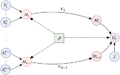
Figure 1: The graphic depicts the causal structure represented as a Directed Acyclic Graph (DAG) associated with the communication task for the multipartite $\mathcal{IC}$ criterion (8), entailing $N-1$ senders and a receiver. The parties have access to a pre-shared entangled quantum state $\rho$ (green square). The senders $\{\mathcal{A}_{k}\}^{N-1}_{k=1}$ receive inputs $\{\{X^{k}_{j}\}^{n}_{j=1}\}^{N-1}_{k=1}$ (blue disks), and transmit messages $\{M_{k}\}^{N-1}_{k=1}$ (pink disks) through binary-symmetric noisy classical channels with parameters $\{\epsilon_{k}\}^{N}_{k=1}$, to the receiver $\mathcal{B}$, respectively. Upon receiving the $N-1$ potentially noisy messages $\{M^{\prime}_{k}\}^{N-1}_{k=1}$, the receiver computes guess $G_{j}$ (purple disk) about a joint function $f_{j}(\{X^{k}_{j}\}^{N-1}_{k=1})$, based on a randomly select input $j\in\{1,\ldots n\}$ (green disk).

Multipartite information causality:— Consider a communication task entailing $N$ spatially separated parties wherein $N-1$ senders $\{\mathcal{A}_{k}\}^{N-1}_{k=1}$ transmit information to a receiver $\mathcal{B}$. Similar to the $(n\mapsto m)$ RAC, each sender $\mathcal{A}_{k}$ receives an $n$-bit string $\mathbf{x}^{k}=(X_{1}^{k},X_{2}^{k},\cdots,X_{n}^{k})$ as input which is encoded on to a $m<n$-bit classical message $M_{k}$ and transmitted to $\mathcal{B}$ via a potentially noisy communication channel with capacity $C_{k}<m$. $\mathcal{B}$ in turn gets the noisy messages $\{M_{k}^{\prime}\}$, and based on randomly chosen input $j\in\{1,\ldots,n\}$ he produces a guess $G_{j}$ about a function of the form $f_{j}(X_{j}^{1},X_{j}^{2},\cdots,X_{j}^{N-1})$. The directed acyclic graph representing the causal structure associated with this communication task in presented in Figure 1. Observe that in contrast to bipartite $(n\mapsto m)$ RAC wherein $\mathcal{B}$ attempts to guess a randomly chosen bit of $\mathcal{A}$, this task is multipartite, as $\mathcal{B}$ guesses a joint function $f_{j}$ of the $j$th input bits of the $N-1$ senders $\{\mathcal{A}_{k}\}^{N-1}_{k=1}$. Consequently, the bipartite criteria of $\mathcal{IC}$ presented above (6) and (7) fail to discard post-quantum correlations in this set-up. Instead, let us consider the following multipartite criterion for $\mathcal{IC}$,

$$\sum_{k,i}I(X_{i}^{k}:X_{i}^{1},\dots,X_{i}^{k-1},X_{i}^{k+1},\dots,X_{i}^{N-1},\mathbf{M^{\prime}},G_{i})\\ \leq\sum_{k=1}^{N-1}C_{k}+\sum_{i=1}^{n}I(X_{i+1}^{k},\dots,X_{n}^{k}:X_{i}^{k}).$$ (8)

where $\mathbf{M^{\prime}}=(M_{1}^{\prime},M_{2}^{\prime},\cdots,M_{N-1}^{\prime})$ denotes the tuple of the messages reaching the receiver through the $N$ potentially noisy classical channels. Note that, the criterion (8) generalizes the once presented in [17] by allowing for noisy classical communication. In the supplementary material, we show that it is satisfied by theories, including classical and quantum theory, which satisfy the information theoretic axioms of $\mathcal{IC}$.

In contrast to bipartite criteria (6), (7), the multipartite criterion (8) for $\mathcal{IC}$ forbids stronger than quantum no-signaling correlations in this set-up (Figure 1). Specifically, let us consider the simplest tripartite version of the multipartite communication task presented above, with $N=3$ and $n=2$. Let the two senders $\mathcal{A},\mathcal{E}$ and the receiver $\mathcal{B}$ share a tripartite no-signaling correlation $p(a,b,e|x,y,z)$ satisfying $a\oplus b\oplus e=xy\oplus zy$. $\mathcal{A},\mathcal{E}$ input uncorrelated bits $x=X_{0}^{1}\oplus X_{1}^{1}$, $z=X_{0}^{2}\oplus X_{1}^{2}$, and transmit the message $M_{1}=a\oplus x_{0}^{1}$ and $M_{2}=e\oplus x_{0}^{2}$ via noiseless communication channels such that $C_{1}=C_{2}=1$, respectively. Upon receiving the messages $\{M_{k}\}^{2}_{k=1}$, $\mathcal{B}$ then inputs $y=j-1$ and produces the guess $G_{j}=M_{1}\oplus M_{2}\oplus b$. Consequently, we have that $I(X_{i}^{k}:X_{i}^{3-k},M_{1},M_{2},G_{i})=C_{k}=1$, and $I(X_{i+1}^{k},\dots,X_{n}^{k}:X_{i}^{k})=0$ for all $k,i\in\{1,2\}$, which violates the multipartite $\mathcal{IC}$ criterion (8), thereby, discarding the no-signaling correlation. We are now prepared to test whether non-trivial monogamy relations of the form (2) can be derived from the bipartite (6),(7) and multiparty (8) criteria for $\mathcal{IC}$.

Optimal slice:— To retrieve monogamy relations of the form (2), we need to find the maximum value of $\beta(\mathcal{B},\mathcal{E})$ given $\beta(\mathcal{A},\mathcal{B})$ over all tripartite no-signaling correlations which satisfy the respective non-linear and protocol-dependent $\mathcal{IC}$ criteria. Since the convex polytope of tripartite no-signaling correlations has $53856$ extremal points, these optimization problems are particularly complex. We now present a useful Lemma which significantly reduces this complexity and allows us to restrict to a two-parameter slice of the tripartite no-signaling polytope,

Lemma 1

To find the maximum value of $\beta(\mathcal{B},\mathcal{E})$ given $\beta(\mathcal{A},\mathcal{B})$ permitted by the $\mathcal{IC}$ criteria (6),(7),(8) it suffices to consider tripartite no-signaling correlations $p(a,b,e|x,y,z)$ of the form,

$$p(a,b,e|x,y,z)=\alpha\frac{1}{4}\delta_{a\oplus b,xy}+\gamma\frac{1}{4}\delta_{e\oplus b,zy}+\\ +(1-\alpha-\gamma)1/8,$$ (9)

where $\alpha,\gamma\in[0,1]$ are convex coefficients of the PR-box correlations shared between $(\mathcal{A},\mathcal{B})$ and $(\mathcal{B},\mathcal{E})$, respectively, such that $\alpha+\gamma\leq 1$.

The proof follows from the data-processing inequality and has been deferred to the supplementary material for brevity. Notice that, for any point on the optimal slice specified by $\{\alpha,\gamma\}$ (9) the values CHSH functionals are specified as $\beta(\mathcal{A},\mathcal{B})=\frac{1+\alpha}{2}$ and $\beta(\mathcal{B},\mathcal{E})=\frac{1+\gamma}{2}$. Hence, our problem reduces to finding the maximum $\gamma$ given $\alpha$, such that the correlation (9) satisfies the $\mathcal{IC}$ criteria (6),(7),(8). These problems can now be efficiently tackled numerically, up to machine precision, as we describe below. We plot the resultant curves in Figure 2. First, we discuss the case of the original (6) and the generalized (7) bipartite $\mathcal{IC}$ criteria.

Trivial monogamy from bipartite $\mathcal{IC}$:— Since the criteria (6) and (7) are essentially bipartite, a tripartite no-signaling correlation $p(a,b,e|x,y,z)$ must be locally post-processed into an effectively bipartite correlation $\tilde{p}(a^{\prime},b^{\prime}|x^{\prime},y^{\prime})$. Moreover, we need only consider deterministic post-processing schemes, referred to as wirings. A wiring is completely specified by the choice of the bipartition, for instance $\mathcal{A}$ and $\mathcal{B}^{\prime}\equiv(\mathcal{B},\mathcal{E})$, and the functions,

$$x =F_{1}(x^{\prime}), a^{\prime}= F_{2}(a),$$ (10)

$$y =F_{3}(y^{\prime},z,e), z= F_{4}(y^{\prime}),\> b^{\prime} =F_{5}(b,e),$$

where, $F_{i}:\{0,1\}^{n}\mapsto\{0,1\},\;\forall i\in\{1,2,3,4,5\}$. We note here that the grouped parties $\mathcal{B},\mathcal{E}$ may signal to each other. Consequently, a tripartite correlation $p(a,b,e|x,y,z)$ violates the bipartite criterion (7) for $\mathcal{IC}$, if there exists some wiring that produces an effectively bipartite correlation $\tilde{p}(a^{\prime},b^{\prime}|x^{\prime},y^{\prime})$ which violates it. In fact, such an approach has previously been used to study $\mathcal{IC}$ in multipartite Bell scenarios [14, 16, 32]. In particular, [18, 19, 20] claimed to have derived the quantum monogamy relation (5) through the bipartite $\mathcal{IC}$ criteria (6) by employing a wiring of the form (10). Contrary to these claims, we find that even the generalized $\mathcal{IC}$ criterion does not imply stronger-than-no-signaling monogamy relations, for any wiring of the form (10).

Specifically, for all tripartite correlations $p(a,b,e|x,y,z)$ of the form (9) with $\alpha,\beta\in[0,1]$, we consider all possible wirings of the form (10), to retrieve the effectively bipartite correlations $\tilde{p}(a^{\prime},b^{\prime}|x^{\prime},y^{\prime})$. Then, for each such $\tilde{p}(a^{\prime},b^{\prime}|x^{\prime},y^{\prime})$, we employ the aforementioned protocol for the $(2\mapsto 1)$ RAC, with a binary symmetric noisy communication channel which flips the message bit $M$ with a probability $p(M^{\prime}=M\oplus 1|M)=\epsilon\in(1/2,1]$ for $M\in\{0,1\}$. Paralleling the observation in [15], we find that the tightest bounds on the maximum of value $\gamma$ given $\alpha\in[0,1]$ are recovered as $\epsilon\rightarrow 1/2$. We plot the resultant monogamy relation in Figure 2. The bipartite $\mathcal{IC}$ criteria (6),(7) retrieve the Tsirelson’s bounds, such that $\beta(\mathcal{B},\mathcal{E})\leq\beta_{Q}=\frac{1}{2}(1+\frac{1}{\sqrt{2}})$ for $\beta(\mathcal{A},\mathcal{B})\in[1/2,\frac{1}{2}(1-\frac{1}{\sqrt{2}})]$. However, for $\beta(\mathcal{A},\mathcal{B})\in[\frac{1}{2}(1-\frac{1}{\sqrt{2}}),\beta_{Q}]$ the monogamy relation implied by these criteria coincides with the no-signaling monogamy relation (4) such that, $\beta(\mathcal{B},\mathcal{E})\leq\frac{3}{2}-\beta(\mathcal{A},\mathcal{B})$. In particular, when $\mathcal{A},\mathcal{B}$ observe the Tsirelson’s bound $\beta(\mathcal{A},\mathcal{B})=\beta_{Q}$, the bipartite criteria (6),(7) fail to retrieve the quantum monogamy $\beta(\mathcal{B},\mathcal{E})\leq\frac{1}{2}$, as they allow for $\beta(\mathcal{B},\mathcal{E})\leq\frac{1}{2}(1-\frac{1}{\sqrt{2}})$. Thus, we conclude that the original (6) and generalized (7) bipartite criteria for $\mathcal{IC}$ fail to yield non-trivial monogamy relations beyond no-signaling. Let us now consider the multipartite $\mathcal{IC}$ criterion (8).

Non-trivial monogamy from multipartite $\mathcal{IC}$:— For each tripartite correlation $p(a,b,e|x,y,z)$ of the form (9), we use the protocol for simplest $(N=3,n=2)$ multipartite communication task described above. Furthermore, we consider independent binary symmetric noisy classical channels between $\mathcal{A},\mathcal{B}$ and $\mathcal{E},\mathcal{B}$, respectively, which flip the input with probability $p(M^{\prime}_{1}=M_{1}\oplus 1|M_{1})=\epsilon_{1}$ and $p(M^{\prime}_{2}=M_{2}\oplus 1|M_{1})=\epsilon_{2}$, such that multipartite $\mathcal{IC}$ criterion (8) translates to,

$$\sum^{2}_{k=1}\sum^{2}_{j=1}I(X_{j}^{k}:X_{j}^{3-k},M_{1}^{\prime},M_{2}^{\prime},G_{j})\leq 2-\sum^{2}_{k=1}h(1-\epsilon_{k}).$$ (11)

In contrast to the bipartite $\mathcal{IC}$ criteria (6),(7), we find that there exists correlations of the form (9), which satisfy the no-signalling monogamy relation (4), but violate the tripartite $\mathcal{IC}$ criterion (11) for some $\epsilon_{1},\epsilon_{2}\in(1/2,1]$. In other words, the tripartite $\mathcal{IC}$ criterion (11) implies a non-trivial monogamy relation of the form (1), which we plot in Figure 2. Most significantly, when $\mathcal{A},\mathcal{B}$ observe the Tsirelson’s bound $\beta(\mathcal{A},\mathcal{{B}})=\frac{1}{2}(1+\frac{1}{\sqrt{2}})$, the criterion (11) is violated for all $\beta(\mathcal{B},\mathcal{E})>1/2$, up to machine precision. This forms our first result,

Result 1

For $\beta(\mathcal{A},\mathcal{{B}})=\beta_{Q}$, the tripartite $\mathcal{IC}$ criterion (11) recovers the quantum monogamy (5) implying that $\mathcal{B}$ must be completely uncorrelated with the third party $\mathcal{E}$, such that, $\beta(\mathcal{B},\mathcal{E})=1/2$.

Moreover, the criterion (11) retrieves tighter than no-signaling monogamy relations for $\beta(\mathcal{A},\mathcal{B})\in[0.8333,\beta_{Q}]$. We now demonstrate that the monogamy relation implied by (11), although weaker than the quantum monogamy relation (5), is strong enough to enhance the information theoretic security of DIQKD protocols.

Secure DIQKD from $\mathcal{IC}$:— Recall that the generic monogamy relations of the form (2) can be used to derive the condition (3) for ensuring security of DIQKD protocol based on the CHSH scenario against individual attach of an eavesdropper constrained by a nonlocal theory $T$ [22, 6, 23, 24]. In Figure 2, we plot the condition (3) for ensuring security of DIQKD protocol. Observe that neither the no-signaling condition (4) nor the bipartite criteria (6),(7) yield security for realizable quantum correlations $\beta(\mathcal{A},\mathcal{B})\leq\beta_{Q}$. However, we find that the tripartite criterion (11) ensures secure DIQKD for a range of realizable quantum correlations, which forms our final result,

Result 2

For $\beta(\mathcal{A},\mathcal{B})\in[0.8471,\beta_{Q}]$, the monogamy relation implied by the tripartite $\mathcal{IC}$ criterion (11) satisfies the criterion (3), thereby, ensuring the security of DIQKD against no-signaling adversaries constrained by $\mathcal{IC}$.

Summarizing, we established formal connections between $\mathcal{IC}$ and monogamy of nonlocality. Specifically, we considered monogamy relations of the form (2) in the simplest tripartite Bell scenario. We used Lemma (1) to restrict to a two-parameter slice of the tripartite no-signaling polytope, on which we evaluated the $\mathcal{IC}$ criteria (6),(7),(8), to retrieve the implied monogamy relations (Figure 2). We remark here that since Lemma (1) holds for any informational criteria which satisfy the data-processing inequality, it opens the way for efficient evaluation of $\mathcal{IC}$ criteria beyond the ones considered here. We find that the bipartite criteria (6),(7) fail to retrieve a monogamy relation beyond no-signaling. Nevertheless, we demonstrate that the multipartite $\mathcal{IC}$ criteria (8),(11) can retrieve non-trivial monogamy relation stricter than the one implied by the no-signaling condition (4). Finally, we use this monogamy relation to demonstrate that the informational constraints implied by $\mathcal{IC}$ ensure the information theoretic security of realizable DIQKD protocols against individual attacks of an adversary.

Notably, the tripartite $\mathcal{IC}$ criterion (11) retrieves the quantum bound on $\beta({\mathcal{B},\mathcal{E}})$ when $\beta(\mathcal{A},\mathcal{B})=\beta_{Q}$. However, there remains a gap between the bounds implied by (11) and quantum monogamy (5), on $\beta_{\mathcal{B},\mathcal{E}}$ for the general case $\beta_{\mathcal{A},\mathcal{B}}\in(0.5,\beta_{Q})$. Owing to the inherent protocol-dependent formulation of the $\mathcal{IC}$ criteria, it remains an open question if this gap can be closed by employing different protocols, non-binary-symmetric noisy classical channels, or other $\mathcal{IC}$ criteria. Finally, it is interesting to explore the extension of our results to monogamy relations between other Bell inequalities in larger Bell scenarios.

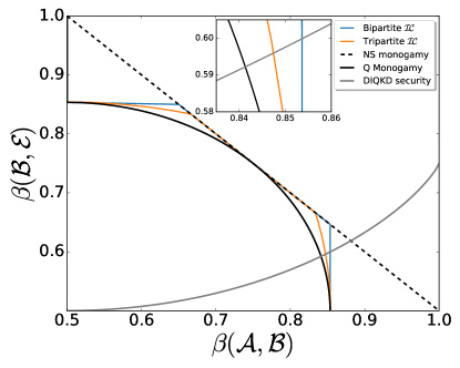
Figure 2: A plots of the maximum value of the CHSH functional $\beta(\mathcal{B},\mathcal{E})$ implied by the monogamy relations (of the form (2)) considered in this work, against the CHSH functional $\beta(\mathcal{A},\mathcal{B})\in[1/2,1]$. The dashed and solid black lines represent the monogamy relations implied by the no-signaling condition (4) and quantum theory (5), respectively. The solid blue line represents monogamy relation implied by the bipartite $\mathcal{IC}$ criteria (6),(7) taking into account all possible wiring of the form (10). The solid orange line represents the monogamy relation implied by the tripartite $\mathcal{IC}$ criterion (11). Finally, the solid gray line exhibits the security condition (3) for DIQKD. Notice that, in contrast to the bipartite criterion, the tripartite $\mathcal{IC}$ criterion implies a non-trivial monogamy relation for $\beta(\mathcal{A},\mathcal{B})\in[0.8333,\beta_{Q}=\frac{1}{2}(1+\frac{1}{\sqrt{2}})$, and ensures security of DIQKD for $\beta(\mathcal{A},\mathcal{B})\in[0.8471,\beta_{Q}]$.

We thank Rafael Rabelo for fruitful discussions and suggestions. This study was financed in part by the Coordenação de Aperfeiçoamento de Pessoal de Nível Superior - Brasil (CAPES) - Finance Code 001 - and by the Brazilian National Council for Scientific and Technological Development (CNPq). This work was partially supported by the Foundation for Polish Science (IRAP project, ICTQT, contract No. MAB/218/5, co-financed by EU within the Smart Growth Operational Programme). AC acknowledges financial support by NCN grant SONATINA 6 (contract No. UMO-2022/44/C/ST2/00081). C.R acknowledges support from the Narodowe Centrum Nauki (NCN) (SHENG project, contract No. 2018/30/Q/ST2/00625) and partially by the National Centre for Research and Development (QuantERA project, contract no. QUANTERA/2/2020). P.R.D acknowledges support from the NCN Poland, ChistEra-2023/05/Y/ST2/00005 under the project Modern Device Independent Cryptography (MoDIC).

Supplementary Material

In this appendix, we provide proofs for the updated version of multipartite information causality ($\mathcal{IC}$) introduced in the equation (8) and Lemma 1. The main ingredient of this proof is an axiom of $\mathcal{IC}$, namely, the data processing inequality, which states that any local manipulation of data can only decay information, and is expressed as,

$$I(A:B)\geq I(A:B^{\prime}),$$ (12)

where $I(A:B)$ is an abstract theory independent mutual information between systems $A,B$, and $B^{\prime}$ is obtained from $B$ via a local transformation.

Proof of multipartite $\mathcal{IC}$ criterion (8)

As the $\mathcal{IC}$ criterion (7) generalizes the multipartite criterion in Eq. (8) in [17] by including the messages $\mathbf{M^{\prime}}\equiv\{M^{\prime}_{k}\}^{N-1}_{k=1}$, the proof closely follows the proof presented in Appendix B of [17]. Apart from the data-processing inqeuality (12) we also invoke the other two theory-independent axioms of $\mathcal{IC}$ in this proof, namely, consistency and the chain-rule presented in [12]. With the multipartite communication scenario depicted in Figure 1, let us consider the mutual information quantity $I(\mathbf{x}^{k}:\mathbf{x}^{1},\cdots,\mathbf{x}^{k-1},\mathbf{x}^{k+1},\cdots,\mathbf{x}^{N-1},\mathbf{M^{\prime}},c)$ which provides a measure of the entire network’s knowledge about the data set of part $k$. Using the relation provided in Eq. (B8) from [17], we derive the left-hand side of (8) in the following way,

$$I(\mathbf{x}^{k}:\mathbf{x}^{1},\cdots,\mathbf{x}^{k-1},\mathbf{x}^{k+1},\cdots,\mathbf{x}^{N-1},\mathbf{M^{\prime}},c)\\ \geq\sum_{i=1}^{n}I(X_{i}^{k}:X_{i}^{1},X_{i}^{2},\cdots,X_{i}^{k-1},X_{i}^{k+1},\cdots,X_{i}^{N-1},\mathbf{M^{\prime}},c)-\sum_{i=1}^{n}I(X_{i+1}^{k},\cdots,X_{n}^{k}:X_{i}^{k}).$$ (13)

Given that $\mathbf{M^{\prime}}$ are classical variables, we use the data processing inequality (12) to refine the above inequality as,

$$I(\mathbf{x}^{k}:\mathbf{x}^{1},\cdots,\mathbf{x}^{k-1},\mathbf{x}^{k+1},\cdots,\mathbf{x}^{N-1},\mathbf{M^{\prime}},c)\\ \geq\sum_{i=1}^{n}I(X_{i}^{k}:X_{i}^{1},X_{i}^{2},\cdots,X_{i}^{k-1},X_{i}^{k+1},\cdots,X_{i}^{N-1},\mathbf{M^{\prime}},G_{i})-\sum_{i=1}^{n}I(X_{i+1}^{k},\cdots,X_{n}^{k}:X_{i}^{k}).$$ (14)

Next, we derive an upper bound on $I(\mathbf{x}^{k}:\mathbf{x}^{1},\cdots,\mathbf{x}^{k-1},\mathbf{x}^{k+1},\cdots,\mathbf{x}^{N-1},\mathbf{M^{\prime}},c)$ by decomposing $\mathbf{M^{\prime}}$ into $M_{1}^{\prime},\cdots,M_{k}^{\prime},\cdots,M_{N-1}^{\prime}$ and applying the chain rule, to obtain,

$$I(\mathbf{x}^{k}:\mathbf{x}^{1},\cdots,\mathbf{x}^{k-1},\mathbf{x}^{k+1},\cdots, \mathbf{x}^{N-1},M_{1}^{\prime},\cdots,M_{k}^{\prime},\cdots,M_{N-1}^{\prime},c)$$ (15)

$$= I\>(\mathbf{x}^{k}:M_{k}^{\prime}|\mathbf{x}^{1},\cdots,\mathbf{x}^{k-1},\mathbf{x}^{k+1},\cdots,\mathbf{x}^{N-1},M_{1}^{\prime},\cdots,M_{k-1}^{\prime},M_{k+1}^{\prime},\cdots,M_{N-1}^{\prime},c)$$

$$+I(\mathbf{x}^{k}:\mathbf{x}^{1},\cdots,\mathbf{x}^{k-1},\mathbf{x}^{k+1},\cdots,\mathbf{x}^{N-1},M_{1}^{\prime},\cdots,M_{k-1}^{\prime},M_{k+1}^{\prime},\cdots,M_{N-1}^{\prime},c).$$

The second term on the right-hand side vanishes due to the no-signaling assumption. Applying the chain rule to the remaining term and using the non-negativity of mutual information $I(A:B)\geq 0$, we get

$$I(\mathbf{x}^{k}:\mathbf{x}^{1},\cdots,\mathbf{x}^{k-1},\mathbf{x}^{k+1},\cdots,\mathbf{x}^{N-1},M_{1}^{\prime},\cdots,M_{k}^{\prime},\cdots,M_{N-1}^{\prime},c)\\ \leq I(M_{k}^{\prime}:\mathbf{x}^{1},\cdots,\mathbf{x}^{k},\cdots,\mathbf{x}^{N-1},M_{1}^{\prime},\cdots,M_{k-1}^{\prime},M_{k+1}^{\prime},\cdots,M_{N-1}^{\prime},c).$$ (16)

Applying the data processing inequality (12) again, we know that including $M_{k}$ in the right-hand side can only increase the mutual information,

$$I(\mathbf{x}^{k}:\mathbf{x}^{1},\cdots,\mathbf{x}^{k-1},\mathbf{x}^{k+1},\cdots,\mathbf{x}^{N-1},M_{1}^{\prime},\cdots,M_{k}^{\prime},\cdots,M_{N-1}^{\prime},c)\\ \leq I(M_{k}^{\prime}:\mathbf{x}^{1},\cdots,\mathbf{x}^{k},\cdots,\mathbf{x}^{N-1},M_{1}^{\prime},\cdots,M_{k-1}^{\prime},M_{k+1}^{\prime},\cdots,M_{N-1}^{\prime},c,M_{k}).$$ (17)

From the causal structure depicted in Figure 1, it is clear that $M_{k}$ shields $M_{k}^{\prime}$ from all other variables $\mathbf{V}$, such that $\;I(M_{k}^{\prime}:\mathbf{V}|M_{k})=I(M_{k}^{\prime}:\mathbf{V},M_{k})-I(M_{k}^{\prime}:M_{k})=0$. Thus, we simplify the inequality (17) as,

$$I(\mathbf{x}^{k}:\mathbf{x}^{1},\cdots,\mathbf{x}^{k-1},\mathbf{x}^{k+1},\cdots,\mathbf{x}^{N-1},M_{1}^{\prime},\cdots,M_{k}^{\prime},\cdots,M_{N-1}^{\prime},c)$$ (18)

$$\leq I(M_{k}^{\prime}:M_{k})=C_{k}.$$ (19)

Finally, by combining (14) and (18), and summing over all $k$, we recover the $\mathcal{IC}$ criterion (8) presented in the main text,

$$\sum_{k=1}^{N-1}\sum_{i=1}^{n}I(X_{i}^{k}:X_{i}^{1},\dots,X_{i}^{k-1},X_{i}^{k+1},\dots,X_{i}^{N-1},\mathbf{M^{\prime}},G_{i})\leq\sum_{k=1}^{N-1}C_{k}+\sum_{k=1}^{N-1}\sum_{i=1}^{n}I(X_{i+1}^{k},\dots,X_{n}^{k}:X_{i}^{k}).$$ (20)

Proof of Lemma 1

In this section, we present the proof of Lemma 1. Specifically, we demonstrate that the slice (9) is optimal for retrieving monogamy relations of the form (2) from bipartite and multipartite criteria (6),(7),(11) for information causality ($\mathcal{IC}$) in a tripartite $\mathcal{A},\mathcal{B},\mathcal{E}$ binary input $x,y,z\in\{0,1\}$ and binary output $a,b,e\in\{0,1\}$ Bell scenario.

Recall that, our aim is to retrieve upper bounds on the value CHSH expression $\beta(\mathcal{B},\mathcal{E})$ between $\mathcal{B}$,$\mathcal{E}$ as a function of the (for a given) value of CHSH expression $\beta(\mathcal{A},\mathcal{B})$ between Alice and Bob. To this end, we observe that $\beta(\mathcal{A},\mathcal{B})$ and $\beta(\mathcal{B},\mathcal{E})$ are individually maximized by their respective PR-boxes $\text{PR}_{\mathcal{A}\mathcal{B}}\otimes L_{\mathcal{E}},\text{PR}_{\mathcal{B}\mathcal{E}}\otimes L_{\mathcal{A}}$ where $L_{\mathcal{A}},L_{\mathcal{E}}$ are some local distributions for $\beta(\mathcal{A},\mathcal{E})$, respectively, such that,

$$p_{\text{PR}_{\mathcal{A}\mathcal{B}}\otimes L_{\mathcal{E}}}(a,b,e|x,y,z)=\frac{1}{2}\delta_{a\oplus b,xy}p_{L_{\mathcal{E}}}(e|z),$$ (21)

$$p_{\text{PR}_{\mathcal{B}\mathcal{E}}\otimes L_{\mathcal{A}}}(a,b,e|x,y,z)=\left(\frac{1}{2}\delta_{b\oplus e,yz}\right)p_{L_{\mathcal{A}}}(a|x),$$ (22)

respectively. We note here that the product structure of these correlations follows from the respective no-signaling conditions. Specifically, the no-signaling condition forces the tripartite distribution to factorize whenever any two of the three parties share a PR-box.

As, in the tripartite binary input and binary output Bell scenario, any other extremal nonlocal tripartite no-signaling box cannot attain the maximal violation of the CHSH inequalities [34], its contribution can be effectively ignored. Consequently, without loss generality, we can restrict ourselves to considering a correlation $\mathbb{P}^{(\alpha,\gamma)}_{\mathcal{A}\mathcal{B}\mathcal{E}}$ formed a convex combination of correlations $\text{PR}_{\mathcal{A}\mathcal{B}}\otimes L_{\mathcal{E}}$ (21), $\text{PR}_{\mathcal{B}\mathcal{E}}\otimes L_{\mathcal{A}}$ (22) and a product distribution $\mathbb{P}_{\mathcal{A}}\otimes\mathbb{P}_{\mathcal{B}}\otimes\mathbb{P}_{\mathcal{E}}$ composed of the marginal distributions such that, $\mathbb{P}^{(\alpha,\gamma)}_{\mathcal{A}\mathcal{B}\mathcal{E}}=\alpha\text{PR}_{\mathcal{A}\mathcal{B}}\otimes L_{\mathcal{E}}+\gamma\text{PR}_{\mathcal{B}\mathcal{E}}\otimes L_{\mathcal{A}}+(1-\alpha-\gamma)\mathbb{P}^{(\alpha,\gamma)}_{\mathcal{A}}\otimes\mathbb{P}^{(\alpha,\gamma)}_{\mathcal{B}}\otimes\mathbb{P}^{(\alpha,\gamma)}_{\mathcal{E}}$, where the coefficients $\alpha,\gamma\geq 0$, $\alpha+\gamma\leq 1$, such that,

$$p_{\mathbb{P}^{(\alpha,\gamma)}_{\mathcal{A}\mathcal{B}\mathcal{E}}}(a,b,e|x,y,z)=\alpha p_{\text{PR}_{\mathcal{A}\mathcal{B}}\otimes L_{\mathcal{E}}}(a,b,e|x,y,z)+\gamma p_{\text{PR}_{\mathcal{B}\mathcal{E}}\otimes L_{\mathcal{A}}}(a,b,e|x,y,z)+(1-\alpha-\gamma)p_{\mathbb{P}^{(\alpha,\gamma)}_{\mathcal{A}}}(a|x)p_{\mathbb{P}^{(\alpha,\gamma)}_{\mathcal{B}}}(b|y)p_{\mathbb{P}^{(\alpha,\gamma)}_{\mathcal{E}}}(e|z),$$ (23)

where,

$$p_{\mathbb{P}^{(\alpha,\gamma)}_{\mathcal{A}}}(a|x)=\frac{1}{\alpha+\gamma}\sum_{b,e\in\{0,1\}}\left(\alpha p_{\text{PR}_{\mathcal{A}\mathcal{B}}\otimes L_{\mathcal{E}}}(a,b,e|x,y,z)+\gamma p_{\text{PR}_{\mathcal{B}\mathcal{E}}\otimes L_{\mathcal{A}}}(a,b,e|x,y,z)\right)=\frac{1}{2},$$ (24)

$$p_{\mathbb{P}^{(\alpha,\gamma)}_{\mathcal{B}}}(b|y)=\frac{1}{\alpha+\gamma}\sum_{a,e\in\{0,1\}}\left(\alpha p_{\text{PR}_{\mathcal{A}\mathcal{B}}\otimes L_{\mathcal{E}}}(a,b,e|x,y,z)+\gamma p_{\text{PR}_{\mathcal{B}\mathcal{E}}\otimes L_{\mathcal{A}}}(a,b,e|x,y,z)\right),$$ (25)

$$p_{\mathbb{P}^{(\alpha,\gamma)}_{\mathcal{E}}}(e|z)=\frac{1}{\alpha+\gamma}\sum_{b,e\in\{0,1\}}\left(\alpha p_{\text{PR}_{\mathcal{A}\mathcal{B}}\otimes L_{\mathcal{E}}}(a,b,e|x,y,z)+\gamma p_{\text{PR}_{\mathcal{B}\mathcal{E}}\otimes L_{\mathcal{A}}}(a,b,e|x,y,z)\right).$$ (26)

Consequently, we have a family of two-parameter slices of tripartite no-signaling polytope characterized by the local distributions $L_{\mathcal{A}},L_{\mathcal{E}}$. In particular, in each of these slices, the value of the CHSH expressions are determined exclusively by the coefficients ${(\alpha,\gamma)}$ such that,

$$\beta(\mathcal{A},\mathcal{B})=\frac{1+\alpha}{2};$$ (27)

$$\beta(\mathcal{B},\mathcal{E})=\frac{1+\gamma}{2}.$$ (28)

Next, we demonstrate that for retrieving monogamy relations of the form (2) for bipartite (6),(7) and multipartite criteria (8),(11) for $\mathcal{IC}$, it is optimal to take the local distributions $L_{\mathcal{A}},L_{\mathcal{E}}$ to be white noise distributions $L_{\mathcal{A}}=\text{\text{WN}}_{\mathcal{A}},L_{\mathcal{E}}=\text{WN}_{\mathcal{E}}$, where,

$$p_{\text{WN}_{\mathcal{A}}}(a|x)=\frac{1}{2}$$ (29)

$$p_{\text{WN}_{\mathcal{E}}}(e|z)=\frac{1}{2}.$$ (30)

To prove the desired thesis, as a starting point, let us consider a tripartite distribution ${\mathbb{P}^{(\alpha,\gamma)}_{\mathcal{A}\mathcal{B}\mathcal{E}}}$ which satisfies the bipartite $\mathcal{IC}$ criterion (7), such that,

$$\sum_{i=1}^{n}I_{{\mathbb{P}^{(\alpha,\gamma)}_{\mathcal{A}\mathcal{B}\mathcal{E}}}}(X_{i}:G_{i},M^{\prime})+\sum_{i=2}^{n}I_{\mathbb{P}^{(\alpha,\gamma)}_{\mathcal{A}\mathcal{B}\mathcal{E}}}(X_{1}:X_{i}|G_{i},M^{\prime})\leq C+\sum_{i=2}^{n}H(X_{i})-H(X_{1},...,X_{n}),$$ (31)

and/or multipartite (8) $\mathcal{IC}$ criterion,

$$\sum_{k,i}I_{{\mathbb{P}^{(\alpha,\gamma)}_{\mathcal{A}\mathcal{B}\mathcal{E}}}}(X_{i}^{k}:X_{i}^{1},\dots,X_{i}^{k-1},X_{i}^{k+1},\dots,X_{i}^{N-1},\mathbf{M^{\prime}},G_{i})\leq\sum_{k}^{N-1}C_{k}+\sum_{i}^{n}I(X_{i+1}^{k},\dots,X_{n}^{k}:X_{i}^{k}),$$ (32)

where we have used the respective protocols described in the main text such that mutual information terms $I_{{\mathbb{P}^{(\alpha,\gamma)}_{\mathcal{A}\mathcal{B}\mathcal{E}}}}$ on the left hand side of (31),(32) depend only on the tripartite correlation $\mathbb{P}^{(\alpha,\gamma)}_{\mathcal{A}\mathcal{B}\mathcal{E}}$. Notice that terms on right hand side of (31),(32) depend only on specifics of the communication task and are independent of the the tripartite correlation $\mathbb{P}^{(\alpha,\gamma)}_{\mathcal{A}\mathcal{B}\mathcal{E}}$ such that they are already equal to the terms on the right hand side of (7),(8). Let us now consider a distribution $\bar{\mathbb{P}}^{(\alpha,\gamma)}_{\mathcal{A}\mathcal{B}\mathcal{E}}$ obtained from the given distribution $\mathbb{P}^{(\alpha,\gamma)}_{\mathcal{A}\mathcal{B}\mathcal{E}}$ by flipping all outputs, such that,

$$p_{\bar{\mathbb{P}}^{(\alpha,\gamma)}_{\mathcal{A}\mathcal{B}\mathcal{E}}}(a,b,e|x,y,z)=\alpha p_{\text{PR}_{\mathcal{A}\mathcal{B}}\otimes\bar{L}_{\mathcal{E}}}(a,b,e|x,y,z)+\gamma p_{\text{PR}_{\mathcal{B}\mathcal{E}}\otimes\bar{L}_{\mathcal{A}}}(a,b,e|x,y,z)+(1-\alpha-\gamma)p_{\bar{\mathbb{P}}^{(\alpha,\gamma)}_{\mathcal{A}}}(a|x)p_{\bar{\mathbb{P}}^{(\alpha,\gamma)}_{\mathcal{B}}}(b|y)p_{\bar{\mathbb{P}}^{(\alpha,\gamma)}_{\mathcal{E}}}(e|z),$$ (33)

where,

$$p_{\bar{L}_{\mathcal{E}}}(e|z)=p_{{L}_{\mathcal{E}}}(e\oplus 1|z),$$

$$p_{\bar{L}_{\mathcal{A}}}(a|x)=p_{{L}_{\mathcal{A}}}(a\oplus 1|x),$$

$$p_{\bar{\mathbb{P}}^{(\alpha,\gamma)}_{\mathcal{B}}}(b|y)=\frac{1}{2},$$

$$p_{\bar{\mathbb{P}}^{(\alpha,\gamma)}_{\mathcal{A}}}(a|x)=p_{{\mathbb{P}}^{(\alpha,\gamma)}_{\mathcal{A}}}(a\oplus 1|x),$$

$$p_{\bar{\mathbb{P}}^{(\alpha,\gamma)}_{\mathcal{E}}}(e|z)=p_{{\mathbb{P}}^{(\alpha,\gamma)}_{\mathcal{E}}}(e\oplus 1|z).$$ (34)

As flipping the outputs is a simple local post-processing, from the data processing inequality (12) we have the following inequality for terms on the left-hand side of (7),

$$\sum_{i=1}^{n}I_{{\bar{\mathbb{P}}^{(\alpha,\gamma)}_{\mathcal{A}\mathcal{B}\mathcal{E}}}}(X_{i}:G_{i},M^{\prime})+\sum_{i=2}^{n}I_{\bar{\mathbb{P}}^{(\alpha,\gamma)}_{\mathcal{A}\mathcal{B}\mathcal{E}}}(X_{1}:X_{i}|G_{i},M^{\prime})\leq\sum_{i=1}^{n}I_{{\mathbb{P}^{(\alpha,\gamma)}_{\mathcal{A}\mathcal{B}\mathcal{E}}}}(X_{i}:G_{i},M^{\prime})+\sum_{i=2}^{n}I_{\mathbb{P}^{(\alpha,\gamma)}_{\mathcal{A}\mathcal{B}\mathcal{E}}}(X_{1}:X_{i}|G_{i},M^{\prime}),$$ (35)

and similarly for the terms on the left-hand side of (8),

$$\sum_{k,i}I_{{\bar{\mathbb{P}}^{(\alpha,\gamma)}_{\mathcal{A}\mathcal{B}\mathcal{E}}}}(X_{i}^{k}:X_{i}^{1},\dots,X_{i}^{k-1},X_{i}^{k+1},\dots,X_{i}^{N-1},\mathbf{M^{\prime}},G_{i})\leq\\ \sum_{k,i}I_{{\mathbb{P}^{(\alpha,\gamma)}_{\mathcal{A}\mathcal{B}\mathcal{E}}}}(X_{i}^{k}:X_{i}^{1},\dots,X_{i}^{k-1},X_{i}^{k+1},\dots,X_{i}^{N-1},\mathbf{M^{\prime}},G_{i}),$$ (36)

while terms on the right-hand side of (7) and (8) depend only on the channel capacity and the prior distribution of the inputs, hence, remain unaltered. Hence, given a distribution which satisfies (7) and/or (8) ${\mathbb{P}}_{\mathcal{A}\mathcal{B}\mathcal{E}}$, the flipped-outcomes distribution $\bar{\mathbb{P}}^{(\alpha,\gamma)}_{\mathcal{A}\mathcal{B}\mathcal{E}}$ also satisfies bipartite (7) and/or multipartite (8) formulations of $\mathcal{IC}$, respectively. Note, that the value of the CHSH expression, $\beta(\mathcal{A},\mathcal{B})$ and $\beta(\mathcal{B},\mathcal{E})$ remain unaltered when all outcomes are simultaneously flipped, as they only depend on the coefficients $(\alpha,\gamma)$ (27) (28).

Now, let us consider another tripartite distribution $\tilde{\mathbb{P}}^{(\alpha,\gamma)}_{\mathcal{A}\mathcal{B}\mathcal{E}}$ obtained by mixing equal proportions of the original tripartite distribution ${\mathbb{P}}^{(\alpha,\gamma)}_{\mathcal{A}\mathcal{B}\mathcal{E}}$ and the flipped-outcomes distribution $\bar{\mathbb{P}}^{(\alpha,\gamma)}_{\mathcal{A}\mathcal{B}\mathcal{E}}$, i.e., $\tilde{\mathbb{P}}^{(\alpha,\gamma)}_{\mathcal{A}\mathcal{B}\mathcal{E}}=\frac{1}{2}({\mathbb{P}}^{(\alpha,\gamma)}_{\mathcal{A}\mathcal{B}\mathcal{E}}+\bar{\mathbb{P}}^{(\alpha,\gamma)}_{\mathcal{A}\mathcal{B}\mathcal{E}})$, such that,

$$p_{\tilde{\mathbb{P}}^{(\alpha,\gamma)}_{\mathcal{A}\mathcal{B}\mathcal{E}}}(a,b,e|x,y,z)=\frac{1}{2}p_{\mathbb{P}^{(\alpha,\gamma)}_{\mathcal{A}\mathcal{B}\mathcal{E}}}(a,b,e|x,y,z)+\frac{1}{2}p_{\bar{\mathbb{P}}^{(\alpha,\gamma)}_{\mathcal{A}\mathcal{B}\mathcal{E}}}(a,b,e|x,y,z),$$ (37)

and specifically,

$$p_{\mathbb{P}^{(\alpha,\gamma)}_{\mathcal{A}\mathcal{B}\mathcal{E}}}(a,b,e|x,y,z) =\alpha p_{\text{PR}_{\mathcal{A}\mathcal{B}}\otimes\text{WN}_{\mathcal{E}}}(a,b,e|x,y,z)+\gamma p_{\text{PR}_{\mathcal{B}\mathcal{E}}\otimes\text{WN}_{\mathcal{A}}}(a,b,e|x,y,z)$$ (38)

$$\ \ \ \ \ \ \ +(1-\alpha-\gamma)p_{\text{WN}_{\mathcal{A}}}(a|x)p_{\text{WN}_{\mathcal{B}}}(b|y)p_{\text{WN}_{\mathcal{E}}}(e|z),$$ (39)

$$=\alpha\frac{1}{4}\delta_{a\oplus b,xy}+\gamma\frac{1}{4}\delta_{b\oplus e,yz}+(1-\alpha-\gamma)1/8,$$ (40)

where for the first equality we have used the facts, $\frac{1}{2}(L_{\mathcal{B}}+\bar{L}_{\mathcal{B}})=\text{WN}_{\mathcal{B}}$, $\frac{1}{2}(L_{\mathcal{E}}+\bar{L}_{\mathcal{E}})=\text{WN}_{\mathcal{E}}$, $\frac{1}{2}(\mathbb{P}^{(\alpha,\gamma)}_{\mathcal{A}}+\bar{\mathbb{P}}^{(\alpha,\gamma)}_{\mathcal{A}})=\text{WN}_{\mathcal{A}}$, $\frac{1}{2}(\mathbb{P}^{(\alpha,\gamma)}_{\mathcal{B}}+\bar{\mathbb{P}}^{(\alpha,\gamma)}_{\mathcal{B}})=\text{WN}_{\mathcal{B}}$, and $\frac{1}{2}(\mathbb{P}^{(\alpha,\gamma)}_{\mathcal{E}}+\bar{\mathbb{P}}^{(\alpha,\gamma)}_{\mathcal{E}})=\text{WN}_{\mathcal{E}}$.

Notice that the values of the CHSH expression, $\beta(\mathcal{A},\mathcal{B})$ and $\beta(\mathcal{B},\mathcal{E})$ still remain unaltered as they only depend on the coefficients $(\alpha,\gamma)$ (27) (28). Now, to complete the proof, all that remains is to demonstrate that if $\mathbb{P}^{(\alpha,\gamma)}_{\mathcal{A}\mathcal{B}\mathcal{E}}$ satisfies the bipartite (7) and/or multipartite (8) $\mathcal{IC}$ criteria for some $(\alpha,\gamma)$, then the corresponding distribution $\tilde{\mathbb{P}}^{(\alpha,\gamma)}_{\mathcal{A}\mathcal{B}\mathcal{E}}$ for the same $(\alpha,\gamma)$ also satisfies the bipartite (7) and/or multipartite (8) formulations of $\mathcal{IC}$. To this end, we invoke convexity of mutual information on probability distributions, which yields, for the bipartite $\mathcal{IC}$ criterion (7),

$$\sum_{i=1}^{n}I_{{\tilde{\mathbb{P}}^{(\alpha,\gamma)}_{\mathcal{A}\mathcal{B}\mathcal{E}}}}(X_{i}:G_{i},M^{\prime})+\sum_{i=2}^{n}I_{\tilde{\mathbb{P}}^{(\alpha,\gamma)}_{\mathcal{A}\mathcal{B}\mathcal{E}}}(X_{1}:X_{i}|G_{i},M^{\prime}) \leq\frac{1}{2}\left(\sum_{i=1}^{n}I_{{{\mathbb{P}}^{(\alpha,\gamma)}_{\mathcal{A}\mathcal{B}\mathcal{E}}}}(X_{i}:G_{i},M^{\prime})+\sum_{i=2}^{n}I_{{\mathbb{P}}^{(\alpha,\gamma)}_{\mathcal{A}\mathcal{B}\mathcal{E}}}(X_{1}:X_{i}|G_{i},M^{\prime})\right)$$

$$\ \ \ \ \ \ \ +\frac{1}{2}\left(\sum_{i=1}^{n}I_{{\bar{\mathbb{P}}^{(\alpha,\gamma)}_{\mathcal{A}\mathcal{B}\mathcal{E}}}}(X_{i}:G_{i},M^{\prime})+\sum_{i=2}^{n}I_{\bar{\mathbb{P}}^{(\alpha,\gamma)}_{\mathcal{A}\mathcal{B}\mathcal{E}}}(X_{1}:X_{i}|G_{i},M^{\prime})\right),$$

$$\leq\sum_{i=1}^{n}I_{{{\mathbb{P}}^{(\alpha,\gamma)}_{\mathcal{A}\mathcal{B}\mathcal{E}}}}(X_{i}:G_{i},M^{\prime})+\sum_{i=2}^{n}I_{{\mathbb{P}}^{(\alpha,\gamma)}_{\mathcal{A}\mathcal{B}\mathcal{E}}}(X_{1}:X_{i}|G_{i},M^{\prime}),$$ (41)

where for the first inequality we have invoked the fact that the mutual information is a convex function of the probability distributions over the protocol-specific variables $\{X_{i}\},\{G_{i}\},M^{\prime}$ which in turn are convex linear functions of the underlying tripartite no-signaling distributions ${\mathbb{P}}^{(\alpha,\gamma)},\bar{\mathbb{P}}^{(\alpha,\gamma)},\tilde{\mathbb{P}}^{(\alpha,\gamma)}$, while the second inequality follows from (35), and similarly for the multipartite $\mathcal{IC}$ criterion (8),

$$\sum_{k,i}I_{{\tilde{\mathbb{P}}_{\mathcal{A}\mathcal{B}\mathcal{E}}}}(X_{i}^{k}:X_{i}^{1},\dots,X_{i}^{k-1},X_{i}^{k+1},\dots,X_{i}^{N-1},\mathbf{M^{\prime}},G_{i}) \leq\frac{1}{2}\sum_{k,i}I_{{{\mathbb{P}}_{\mathcal{A}\mathcal{B}\mathcal{E}}}}(X_{i}^{k}:X_{i}^{1},\dots,X_{i}^{k-1},X_{i}^{k+1},\dots,X_{i}^{N-1},\mathbf{M^{\prime}},G_{i})$$

$$\ \ \ \ +\frac{1}{2}\sum_{k,i}I_{{\bar{\mathbb{P}}_{\mathcal{A}\mathcal{B}\mathcal{E}}}}(X_{i}^{k}:X_{i}^{1},\dots,X_{i}^{k-1},X_{i}^{k+1},\dots,X_{i}^{N-1},\mathbf{M^{\prime}},G_{i})$$

$$\leq\sum_{k,i}I_{{{\mathbb{P}}_{\mathcal{A}\mathcal{B}\mathcal{E}}}}(X_{i}^{k}:X_{i}^{1},\dots,X_{i}^{k-1},X_{i}^{k+1},\dots,X_{i}^{N-1},\mathbf{M^{\prime}},G_{i}),$$ (42)

where for the first inequality we have invoked the fact that the mutual information is a convex function of the probability distributions over the protocol-specific variables $\{X_{i}^{k}\},\{G_{i}\},\mathbf{M^{\prime}}$ which in turn are convex linear functions of the underlying tripartite no-signaling distributions ${\mathbb{P}}^{(\alpha,\gamma)},\bar{\mathbb{P}}^{(\alpha,\gamma)},\tilde{\mathbb{P}}^{(\alpha,\gamma)}$, while the second inequality follows from (36). Yet again, the terms on the right-hand side of (7) and (8) remain unaltered, implying that the distribution $\tilde{\mathbb{P}}^{(\alpha,\gamma)}_{\mathcal{A}\mathcal{B}\mathcal{E}}$ of the desired form (9), satisfies the bipartite (7) and multipartite (8) formulation of $\mathcal{IC}$ while retaining the value of the CHSH expressions (27) (28). This completes the proof, and establishes the optimality of the slice (9).