Chemical Space-Informed Machine Learning Models for Rapid Predictions of X-ray Photoelectron Spectra of Organic Molecules

Abstract

We present machine learning models based on kernel-ridge regression for predicting X-ray photoelectron spectra of organic molecules originating from the ionization energies of 1$s$ electrons in carbon (C), nitrogen (N), oxygen (O), and fluorine (F) atoms. We constructed training dataset through high-throughput calculations of core-electron binding energies (CEBEs) for 12,880 small organic molecules in the bigQM7$\rm{\omega}$ dataset, employing the $\Delta$-SCF formalism coupled with meta-GGA-DFT and a variationally converged basis set. The models are cost-effective, as they require the atomic coordinates of a molecule generated using universal force fields while estimating the target-level CEBEs corresponding to DFT-level equilibrium geometry. We explore transfer learning by utilizing the atomic environment feature vectors learned using a graph neural network framework in kernel-ridge regression. Additionally, we enhance accuracy using the $\Delta$-machine learning framework by leveraging inexpensive baseline spectra derived from Kohn–Sham eigenvalues. Upon application to 208 combinatorially substituted uracil molecules, larger than those in the training set, our analyses reveal that while the models may not yield quantitatively accurate predictions of CEBEs on a molecule-by-molecule basis, they do exhibit a strong linear correlation, which proves valuable for virtual high-throughput screening purposes. We present the dataset and models as the Python module, cebeconf, to facilitate further explorations.

I Introduction

X-ray photoelectron spectroscopy (XPS) distinguishes atoms based on the ionization energies of their core electrons effectively screened by molecular valence electrons. The resulting chemical shifts of core-electron binding energies (CEBEs) enable the identification of the local bonding environment of an atom. A typical XPS spectrum comprises peaks; some merged to form a broader distribution, corresponding to ionized core electrons detected experimentally as photocurrentde Groot and Kotani (2008). The positions and intensities of an XPS spectrum can provide insights on molecular internal coordinatesBagus, Sousa, and Illas (2022), orientation of adsorbates relative to the substrateDiller et al. (2014), chemical compositionAyiania et al. (2020); Feng, Zhou, and Yang (2010), as well as physical conditions such as temperatureDiller et al. (2014); Ayiania et al. (2020) and pressureFeng, Zhou, and Yang (2010).

Advancements in modern synchrotron sources have enabled the precise detection of chemical shifts of CEBEs, achieving a resolution of 0.05 eV Willmott (2019). The precision of 1$s$-CEBEs (denoted hitherto $E_{\rm b}^{1s}$ ) in atoms is limited only by lifetime broadening. In molecular scenario, XPS achieves a precision of $0.1$ eV for $E_{\rm b}^{1s}$ of carbon (C) atomsKovač et al. (2014). For nitrogen (N) and oxygen (O), peak widths of 0.13 and 0.16 eV, respectively, are commonly used in spectral deconvolutionKovač et al. (2014). Theoretical CEBEs of even semi-quantitative accuracy can aid experimental XPS assignmentAzuara-Tuexi, Muñoz-Sandoval, and Guirado-López (2023); Greczynski and Hultman (2020), thereby contributing to diverse applications such as structure elucidationDiller et al. (2014), catalysisTrinh et al. (2018); Nguyen et al. (2019), characterization of energy storage materialsYu et al. (2022), and material composition analysisAzuara-Tuexi, Muñoz-Sandoval, and Guirado-López (2023).

For achieving quantitatively accurate theoretical predictions of XPS, it is crucial to account for core-orbital relaxation effects, which unfold at a sub-femtosecond ($<10^{-15}$ s) timescale mirroring the ultrafast temporal dynamics during experimental detection, resonating with the energy-time uncertainty principlede Groot and Kotani (2008); Kohiki (1999). CEBEs estimated using molecular orbital (MO) energies—based on the Koopmans’ approximationChong, Gritsenko, and Baerends (2002); Azuara-Tuexi, Muñoz-Sandoval, and Guirado-López (2023) in density functional theory (DFT)—show large errors due to the lack of core relaxation in MOs that determine the ground state electronic densityBagus, Ilton, and Nelin (2013); Besley (2021). While many-body methods such as the random phase approximationVoora et al. (2019) and GWGolze, Keller, and Rinke (2020) adequately address screening effects, they are computationally intensive, hence unsuitable for large-scale data generation. Within DFT, alternative approaches such as the Slater transition state method Williams, DeGroot, and Sommers (1975); Jana and Herbert (2023) and the $\Delta$-self consistent field ($\Delta$-SCF ) approach Bagus (1965); Kahk and Lischner (2019); Pueyo Bellafont, Viñes, and Illas (2016) offer promising avenues for incorporating orbital relaxation effects. These methods explicitly account for the vacancy in a core-orbital—i.e., hole—using charge-constraining algorithms such as the maximum-overlap-method Gilbert, Besley, and Gill (2008), thereby preventing the variational collapse of non-Aufbau Slater determinants. While the numerical convergence Carter-Fenk and Herbert (2020) of $\Delta$-SCF is highly coupled to the choice of projectors used for wavefunction localization Klein, Hall, and Maurer (2021); Behler et al. (2007), it emerges as the best option in terms of the overall efficiencyMichelitsch and Reuter (2019); Klein, Hall, and Maurer (2021).

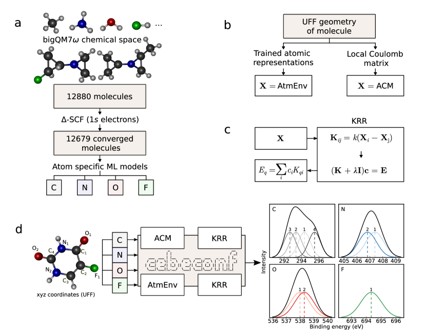
Figure 1: Stepwise workflow of the study: a) DFT structures from the bigQM7$\rm{\omega}$ datasetKayastha, Chakraborty, and Ramakrishnan (2022) were used to generate the bigQM7$\rm{\omega}$ -CEBECONF dataset comprising 85,837 entries of 1$s$-CEBEs ($E_{\rm b}^{1s}$ ) of CONF atoms used to train atom-specific ML models. b) Structures generated using universal force fields (UFF) were used to generate the descriptors (X): AtmEnv obtained from trained neural networks and atomic Coulomb matrix (ACM). c) Kernel-ridge regression (KRR) models trained on bigQM7$\rm{\omega}$ -CEBECONF predicts $E_{\rm b}^{1s}$ of a query molecule using descriptors derived from UFF-level geometries as the input. d) Representative use of cebebconf moduleTripathy et al. (2024) to generate XPS spectra from UFF geometry of a query molecule.

The magnitude of $E_{\rm b}^{1s}$ of an element in its reduced state is lower than its oxidized states. For example, the $E_{\rm b}^{1s}$ (C) of a CH moiety is approximately 285 eVDorey et al. (2018), which in CF, CF₂, CF₃, and CF₃OH is systematically shifted to 288, 291, 293.5, and 295 eV, respectivelyWillmott (2019). Similar trends are revealed in XPS measurements of fluorinated polyethylenesFerraria, da Silva, and do Rego (2003) indicating a systematic variation of $E_{\rm b}^{1s}$ with chemical composition and molecular structure.

Molecular chemical space datasets, such as QM9 Ramakrishnan et al. (2014) and bigQM7$\rm{\omega}$ Kayastha, Chakraborty, and Ramakrishnan (2022) have facilitated the elucidation of structure-property relationships through machine learning (ML) modelingRupp, Ramakrishnan, and Von Lilienfeld (2015). The $\Delta$-MLRamakrishnan et al. (2015a) approach further enhances the accuracy by utilizing inexpensive baseline methodsGupta, Chakraborty, and Ramakrishnan (2021); Watson et al. (2023); Golze et al. (2022). In recent years, ML models have successfully predicted local properties of atoms-in-molecules such as nuclear magnetic resonance (NMR) shielding parametersGupta, Chakraborty, and Ramakrishnan (2021); Shiota, Ishihara, and Mizukami (2024); El-Samman et al. (2024a, b) and acid dissociation constants (pKa)El-Samman et al. (2024a, b), as well as ‘global’ molecular properties such as atomization energiesRamakrishnan et al. (2014), electronic excitation energiesRamakrishnan et al. (2015b); Gupta et al. (2021); Kayastha, Chakraborty, and Ramakrishnan (2022), or frontier MO energy gaps Fediai et al. (2023), demonstrating the effectiveness of ML-aided computational chemistry endeavors Ramakrishnan and von Lilienfeld (2017). ML techniques have found utility in spectroscopic applications for mapping spectroscopic features to structural motifsKotobi et al. (2023); Choudhury, Ramakrishnan, and Ghosh (2024). Specifically, several studies Golze et al. (2022); Aarva et al. (2019); Zarrouk et al. (2024) have explored the prediction of XPS spectra in materials. Earlier works on predicting gas-phase XPS spectra, such as those by Rupp et al.Rupp, Ramakrishnan, and Von Lilienfeld (2015) and Golze et al. Golze et al. (2022), utilized subsets of the extensive QM9 dataset.

The present study explores data-driven modeling of XPS spectra of small organic molecules using the new chemical space dataset, bigQM7$\rm{\omega}$ Kayastha, Chakraborty, and Ramakrishnan (2022), which has a larger number of molecules containing upto 7 CONF atoms than the corresponding subset of QM9, offering greater structural and compositional diversity. The minimum energy structures in bigQM7$\rm{\omega}$ were calculated using the range-separated hybrid DFT method $\omega$B97XDChai and Head-Gordon (2008), thereby enhancing the quality of structures suitable for developing datasets of various properties in a single-point fashion. We report ML models for predicting the XPS spectra of organic molecules at the $\Delta$-SCF level requiring as input inexpensive geometries determined using universal force field (UFF) Rappé et al. (1992). These inexpensive inputs are used to generate light-weight descriptors obtained from graph neural networks (GNNs) and a local version of the Coulomb matrix (CM) descriptorRupp et al. (2012); Rupp, Ramakrishnan, and Von Lilienfeld (2015). Further, we propose using Kohn–Sham (KS) eigenvalues obtained from single-point calculations of neutral molecules as a baseline in $\Delta$-ML, where the models are trained on the deviation of baseline predictions from that of a target-level theoryRamakrishnan et al. (2015a). FIG. 1 illustrates our data generation and ML workflow.

In the following, II.1 compiles details of electronic structure methods used for generating the bigQM7$\rm{\omega}$ -CEBECONF dataset containing 85,837 entries of $E_{\rm b}^{1s}$ for all CONF atoms in the bigQM7$\rm{\omega}$ dataset. In II.2, we discuss a scheme to assign quasi-particle energies to CEBEs based on the Mulliken population scheme. We describe the details of ML for modeling local atomic properties in II.3. In II.4, we gather the details of atomic descriptors. We present our results in III: Evaluation of the DFT method used for data generation (III.1); property trends and data distribution (III.2); and analysis of the performance of ML models (III.3 and III.4). We highlight the transferability of our models by applying them to a class of biomolecules in III.5. Finally, we conclude in section IV, highlighting the features of the ML models presented in this study and their scope for future applications.

II Methodology

II.1 Electronic structure calculations

We performed electronic structure calculations using the all-electron, numerically tabulated atom-centered orbital (NAO) code, FHI-aimsBlum et al. (2009). For training the ML models reported in this study, we selected the bigQM7$\rm{\omega}$ dataset, which has been used for generating datasets of electronic excitation spectraKayastha, Chakraborty, and Ramakrishnan (2022); Majumdar and Ramakrishnan (2024). The molecular structures in bigQM7$\rm{\omega}$ were optimized using the ConnGO approach that preserves the covalent bond connectivities during geometry optimization Senthil, Chakraborty, and Ramakrishnan (2021). For this purpose, the range-separated hybrid DFT method, $\omega$B97XD, was used in combination with the def2TZVP basis set. Since the change in nuclear coordinates have negligible effects on XPS, the minimum energy geometries of neutral ground states were used in all calculations.

For $\Delta$-SCF calculations, we selected the meta-generalized gradient approximation (mGGA) to DFT, SCAN, along with the Tight-Full, basis set. The 1$s$-CEBE ($E_{\rm b}^{1s}$ ) in a $\Delta$-SCF calculation is obtained by subtracting the total energy of the neutral molecule ($E_{\rm mol}$) from that of the corresponding 1$s$ core-ionized cation ($E_{\rm cation}^{1s}$)

$$E_{\rm b}^{1s}=E_{\rm cation}^{1s}-E_{\rm mol}.$$ (1)

We exclusively use NAOs with ‘tight’ integration grids to accurately account for orbital relaxation effects in the cationic states involved in the $\Delta$-SCF calculations. While ‘tight’ settings in FHI-aims have ‘tier 2’ basis functions as default, we selected the highest ‘tier’ possible for each element, i.e., ‘tier 3’ for hydrogen (H) and beyond ‘tier 4’ for CONF atoms. We refer to this basis set as Tight-Full. We have also probed the valence-correlation consistent NAO, NAO-VCC-5Z, which is analogous to Dunning’s cc-pV5ZZhang et al. (2013). Since there is minimal error for core-levels when using large basis sets, core augmentation functions Sarangi et al. (2020); Jana and Herbert (2023) were not utilized.

Holes at core-levels were constrained using the force_occupation_basis keyword in FHI-aims. The corresponding approach is a variant of the maximum overlap method Gilbert, Besley, and Gill (2008), specifying the hole in a quasi-AOMulliken (1955). One can also use the force_occupation_projector, which directly constrains the hole at a specified MO; however, we found the former to be more variationally stableKlein, Hall, and Maurer (2021) making it suitable for automated high-throughput calculations with minimal manual data curation.

Intricate modifications specific to core-level predictions are avoided in the Koopmans’ approximation. Accordingly, the negative of the KS orbital energy, $\varepsilon_{i}$, approximates the 1$s$-CEBEChong, Gritsenko, and Baerends (2002); Klein, Hall, and Maurer (2021)

$$E_{\rm b}^{1s}\approx-\varepsilon_{1s}.$$ (2)

In this work, we calculate $\varepsilon_{1s}$ using the PBE-DFT method and the cc-pVDZ basis set through single point calculations on UFF-level structures obtained using the program OpenbabelO’Boyle et al. (2011). Despite lacking contributions from orbital relaxation effects in the Koopmans’ interpretation Bellafont, Bagus, and Illas (2015); Bagus, Ilton, and Nelin (2013), its relative ease of use makes it an efficient choice as a baseline method in $\Delta$-ML.

GW method is considered the “gold standard” for modeling CEBEsGolze et al. (2022); Li et al. (2022). In particular, the use of contour deformation to evaluate self energy in GW, improves the quasi-particle energies for core-levelsGolze et al. (2018); Golze, Dvorak, and Rinke (2019). Among presently available GW approximations, Hedin shifted GW, $G_{\Delta H}W_{0}$, which introduces a state-specific global shift in the quasiparticle self-consistent equations is the most accurateLi et al. (2022). Hence, in this study we use $G_{\Delta H}W_{0}$ for evaluating the accuracy of $\Delta$-SCF results. In all GW calculations, we used KS–eigenstates obtained using PBE-DFT with cc-pVnZ (n=T,Q,5) basis sets and extrapolated the results to arrive at the basis limit values, following the procedure previously used by Golze et al..Golze, Dvorak, and Rinke (2019); Golze, Keller, and Rinke (2020). For systems exhibiting non-monotonic convergence with basis set size, due to contraction errorsMejia-Rodriguez et al. (2022), we used cc-pV5Z values instead of extrapolated energies. The computational complexity of GW methods, which increases manyfold with basis set size limits its applicability in high-throughput data generation. Therefore, GW calculations were performed only for a small subset of bigQM7$\rm{\omega}$ . We use GW-predicted $E_{\rm b}^{1s}$ for assessing the accuracy $\Delta$-SCF and Koopmans’ approximations based on the mGGA-DFT methods, SCAN and TPSS.

From 12,880 bigQM7$\rm{\omega}$ molecules, we excluded 201 that exhibited non-convergence of density in $\Delta$-SCF calculations. While such calculations can be converged through careful assessments of numerical criteria and localization proceduresMichelitsch and Reuter (2019); Klein, Hall, and Maurer (2021), we excluded these molecules for the sake of consistent numerical settings across the dataset. The resulting XPS dataset consists of 85837 entries of $E_{\rm b}^{1s}$ of the constituent CONF atoms of 12679 molecules obtained using $\Delta$-SCF with the SCAN/Tight-Full method. Of this, a shuffled 80:20 train-test split was chosen for training ML models. Further, to validate the ML models, we explore combinatorially substituted derivatives of pyrimidinones and uracil, resulting in 208 biomolecules. For this set, we have calculated $E_{\rm b}^{1s}$ at the SCAN/Tight-Full level using minimum energy structures determined using the $\omega$B97XD/def2TZVP method as implemented in Gaussian16Frisch et al. (2016). Further, for the validation set, we have calculated Koopmans’ estimations with the PBE/cc-pVDZ method using geometries determined with UFF. In all calculations, we accounted for relativistic effects through the atomic zeroth-order regular approximation (aZORA)van Lenthe, Snijders, and Baerends (1996); Klein, Hall, and Maurer (2021). Since the effect of aZORA on CEBEs is a constant shift, non-relativistic estimations can be corrected a posteriori Pueyo Bellafont, Viñes, and Illas (2016); Golze, Keller, and Rinke (2020); Keller et al. (2020); Li et al. (2022). When applying the $\Delta$-ML models presented in study for new predictions, along with UFF geometry, one must provide the baseline-level CEBEs, which is PBE/cc-pVDZ Koopmans’ estimation determined on UFF geometry. Baseline values without relativistic effects can be corrected by adding the intercepts from Figure S1 of the supporting information (SI).

II.2 Assignment of quasi-particle energy to CEBE

The localization of core-holes is assumed inherently in XPS. However, vibronic fine structure underlying the XPS spectrum sheds insights on the participation of core-level MOs in very-weak bondingKempgens et al. (1997); Myrseth et al. (2002). These splittings can be of the order of milli-eVs and observed in high-precision spectroscopic techniques. Dispersions in CEBEs for chemically equivalent atoms in symmetric molecules such as benzeneMyrseth et al. (2002), acetyleneKempgens et al. (1997), dinitrogenHergenhahn et al. (2001), and others Matz, Nijssen, and Jagau (2023) have been observed. Splittings arising from the coupling of core-levels can also be observed and identified in the one-particle energies obtained from KS-eigenvalues. Experimentally, in the case of benzene, 6 degenerate core levels lead to 4 energy levels spanning a range of 64 meV Myrseth et al. (2002)(see Table S1 of SI). While by definition, the values of $E_{\rm b}^{1s}$ of identical atoms will be similar in $\Delta$-SCF predictions, dispersions in $E_{\rm b}^{1s}$ are captured in quasiparticle energies. Therefore, to map the quasiparticle energies of MOs to the respective $\Delta$-SCF energies for use as a baseline in $\Delta$-ML, we use Mulliken population analysis Mulliken (1955).

For assigning the $k$-th MO to an AO centered on atom $A$, of angular momentum quantum number $l$, we use Mulliken population projected on the MO defined as

$$P_{A,k,l}^{\rm M} = 2\sum_{\mu\in A,\mu\in l}\sum_{\lambda}C_{\mu,k}C_{\lambda,k}S_{\lambda,\mu}.$$ (3)

Here, the summation is performed over all AOs, $\mu$, centered on atom $A$ with angular momentum $l$. Here, $C_{\mu,k}$ and $C_{\lambda,k}$ are elements of the $k$-th KS eigenvector corresponding to the AOs, $\mu$ and $\lambda$, respectively. Further, $S_{\lambda,\mu}$ is an element of the overlap or inner product matrix in the AO representation. For a given $k$, the CEBE corresponds to the atom with a maximal projected population. Consequently, when the population is identical for symmetrically equivalent atoms, they will be assigned the same quasiparticle energy. In the bigQM7$\rm{\omega}$ dataset, using KS eigenvalues at the PBE/cc-pVDZ level, 79 pairs of chemically equivalent atoms were assigned the same KS-eigenvalue in 59 molecules.

II.3 KRR-ML framework for modeling CEBE

Kernel-ridge regression (KRR) is an efficient ML framework for accurately modeling molecular and materials propertiesHansen et al. (2015); Stuke et al. (2019); Rupp et al. (2012). It also facilitates modeling local quasi-atomic properties in molecules such as NMR shielding, CEBE, and partial charges on atomsRupp, Ramakrishnan, and Von Lilienfeld (2015); Gupta, Chakraborty, and Ramakrishnan (2021). In this study, we apply KRR-ML for modeling $E_{\rm b}^{1s}$ . For a query atom, $q$, KRR-ML predicts $E_{\rm b}^{1s}$ according to the following equation.

$$E_{\rm b}^{1s}(q)=\lim_{N\rightarrow\infty}\sum_{i=1}^{N}c_{i}K_{qi},$$ (4)

where the summation on the right side is performed over $N$ training examples, c_i are the regression coefficients obtained through training and $K_{qi}$ is the kernel matrix element evaluated between the query atom $q$ and training atom $i$. An attractive feature of KRR is that the training, i.e., the model optimization, is performed by minimizing a convex function for which linear solvers yield the exact solutionSchölkopf et al. (2002); Ramakrishnan and von Lilienfeld (2017). Accordingly, the regression coefficients are obtained by solving the following equation.

$$\left[\textbf{K}+\lambda\textbf{I}\right]\textbf{c}=\textbf{E}_{\rm b}^{1s},$$ (5)

where K and I are $N\times N$ kernel and identity matrices, respectively, while $\textbf{E}_{\rm b}^{1s}$ is the vector of CEBE values of $N$ training entities. The kernel matrix element, $K_{ij}$, captures the similarity between two training atoms ($i$ and $j$) in the form of a kernel function, $k$, sometimes referred as radial basis functions (RBFs) of the corresponding descriptors, $k({\bf d}_{i},{\bf d}_{j})=k({\bf d}_{i}-{\bf d}_{j})$. For brevity, we define ${\bf d}_{i}-{\bf d}_{j}$ as $D_{ij}$. The choice of the descriptor or the representation vector, ${\bf d}$, is presented in II.4.

In this study, we explore Laplacian (a.k.a. exponential) and Gaussian kernels defined as

$$k^{\rm Laplacian}(D_{ij}) = \exp\left(-||D_{ij}||_{1}/\sigma\right)\,{\rm and}$$

$$k^{\rm Gaussian}(D_{ij}) = \exp\left(-||D_{ij}||_{2}^{2}/2\sigma^{2}\right).$$ (6)

. The Laplacian kernel depends on the $L_{1}$ norm, a.k.a. taxicab norm defined as $||{\bf x}||_{1}=\sum_{i}|x_{i}|$, whereas the Gaussian kernel uses the Euclidean norm defined as $||{\bf x}||_{2}=\sqrt{\sum_{i}x_{i}^{2}}$. There are other definitions of kernels where the pairwise comparison can also be an inner-productSchölkopf et al. (2002), which we do not explore in this study.

The hyperparameters, $\lambda$ (in Eq. 5) and $\sigma$ (in Eq. II.3), modulate the performance of KRR-ML models. The parameter $\lambda$ is a non-negative real number serving two purposesRamakrishnan and von Lilienfeld (2017). For positive values, it introduces a penalty to regularize the magnitudes of the regression coefficients, which is necessary to decrease the impact of outliers on the model’s performance. Another more common scenario is that if there are redundancies in the training set and $K_{ij}$ approaches unity, i.e., K becomes a singular matrix. In such cases, adding the second term, $\lambda{\bf I}$, conditions the linear system defined in Eq. 5. It is important to note that the aforementioned redundancies can occur if the representations lack uniqueness, even for a few training examples. In anticipation of such linear dependencies, in all KRR-ML calculations, we set $\lambda$ as $10^{-4}$.

The kernel width, $\sigma$, determines the width of the kernel-RBFs, thereby governing the spread over training examples for predictions. In a previous workRamakrishnan and von Lilienfeld (2015), a heuristic approach was proposed to determine $\sigma$ by setting the minimum of the off-diagonal elements of ${\bf K}$ to 1/2, $K_{ij}^{\rm min}=1/2$, as a measure of conditioning ${\bf K}$. Accordingly, $\sigma$ can be determined using the maximal value of $D_{ij}$ over a random sample. For Laplacian and Gaussian kernels, one arrives atRamakrishnan and von Lilienfeld (2015, 2017):

$$\sigma_{\rm opt}^{\rm Laplacian}=\frac{D_{ij}^{\rm max}}{\log 2};\quad\sigma_{\rm opt}^{\rm Gaussian}=\frac{D_{ij}^{\rm max}}{\sqrt{2\log 2}}.$$ (7)

Since descriptor differences have non-trivial distributions, for KRR-ML modeling of NMR shielding in the QM9-NMR dataset Gupta, Chakraborty, and Ramakrishnan (2021), better results were reported when using the median of the descriptor differences instead of $D_{ij}^{\rm max}$.

To shed more light on the optimal value of kernel-width for a given target property, we set $K_{ij}^{\rm min}$ to be free parameter, $0<\tau<1$, and determine $\sigma$ as follows:

$$\sigma_{\rm opt}^{\rm Laplacian}=\frac{D_{ij}^{\rm max}}{\log 1/\tau};\quad\sigma_{\rm opt}^{\rm Gaussian}=\frac{D_{ij}^{\rm max}}{\sqrt{2\log 1/\tau}}.$$ (8)

We scanned $\tau$ in the range 0.03 to 0.99 in steps of 0.03.

II.4 Local descriptors for atom-in-molecules

For ML modeling of local properties with KRR, several descriptors or representations have been proposed to describe the atomic environment: Gaussian RBFsBehler and Parrinello (2007), local CMRupp et al. (2012), smooth overlap of atomic positions (SOAP) Szlachta, Bartók, and Csányi (2014), neural network (NN) embeddingsUnke and Meuwly (2018), atomic spectral London-Axilrod-Teller-Muto (aSLATM) Huang and von Lilienfeld (2020), and Faber-Christensen-Huang-Lilienfeld (FCHL)Faber et al. (2018). Formally, many-body RBFs, SOAP, aSLATM, and FCHL are continuous representations placing heavy storage requirements. On the other hand, CM and embeddings are discrete representations amenable to rapid predictions. Since one of the aims of this study is to present ML models pre-trained on a large training set, we have explored atomic CM (ACM) and atomic environment obtained as embeddings by training a GNN (AtmEnv).

As stated before, of the 12,880 molecules in the bigQM7$\rm{\omega}$ dataset, 201 did not converge during $\Delta$-SCF calculations. The remaining 12,679 were partitioned into four subsets based on the presence of C/O/N/F atoms. The subset with ‘C’ was the largest, with 12674 molecules, as ‘C’ is present in all molecules in bigQM7$\rm{\omega}$ but HF, H₂O, NH₃, F₂, and O₂. See Table S2 of supplementary information (SI) for further details.

The target property, $E_{\rm b}^{1s}$ of C/O/N/F atoms were calculated using the minimum energy geometries of the bigQM7$\rm{\omega}$ molecules, previously determined at the $\omega$B97XD/def2TZVP level of theoryKayastha, Chakraborty, and Ramakrishnan (2022). However, to generate local descriptions, we utilize molecular geometries determined using UFF starting from ‘simplified molecular-input line-entry system’ (SMILES) strings. As in previous studiesRamakrishnan et al. (2015a); Gupta et al. (2021), ML models trained using baseline levels such as UFF also capture the change in the structure-property mapping: DFT-property@DFT-geometry $\rightarrow$ DFT-property@UFF-geometry. Training with UFF geometries circumvents computational bottlenecks in DFT-level structure optimization for out-of-sample queries that are more expensive than $\Delta$-SCF calculations of $E_{\rm b}^{1s}$ enabling rapid application of the ML models to new systems.

II.4.1 Atomic CM

CM is one of the simplest structure-based descriptors for mapping atomic coordinates and molecular stoichiometries to a molecular global property such as atomization energyRupp et al. (2012). For a molecule with $N$ atoms, CM is an $N\times N$ matrix defined as

$$M_{ij} = Z_{i}^{2.4}/2;\quad i=j$$ (9)

$$= Z_{i}Z_{j}/R_{ij};\quad i\neq j,$$

where $Z_{i}$ is the atomic number of atom-$i$ while $R_{ij}$ is the Euclidean distance between nuclei $i$ and $j$ in Å. Changing the unit of coordinates will reflect in the kernel-width, $\sigma$. The off-diagonal elements in the CM represent Coulomb interaction between the nuclei of atoms; the diagonal element is an estimation of the atomic total energyRamakrishnan and von Lilienfeld (2017).

The CM is symmetric and invariant to rotation and translation but not to the choice of atomic indices. To make CM atom-index invariant, one can uniquely permute its rows and columns based on a metricVon Lilienfeld (2013). The row-sorted norm version is a popular approachMontavon et al. (2012). The randomly sorted CM approachMontavon et al. (2012) considers different shuffles, included as separate training examples, offering lower prediction errors than the row sorted approachHansen et al. (2013). As CM is symmetric, either the upper or the lower triangular matrix is sufficient to construct the descriptor vector.

In the atomic CM (ACM), each query atom, $q$, is represented by an $N\times N$ matrix. The indices of the $N$ atoms are permuted in ascending order of distances of the neighboring atoms from the query atom, $q$. We do not apply a cut-off radius to determine the neighbor atoms. To ensure that all the entries have the same descriptor size, the size of ACM is allocated to $M\times M$ where $M=23$ is the maximum number of atoms in the bigQM7$\rm{\omega}$ dataset corresponding to $n$-heptane. All elements of the ACM other than the $N\times N$ block are set to zero. The indexing of the atoms for ACM is schematically shown in Figure S2 of SI.

II.4.2 AtmEnv: Descriptor from Graph Neural Network

Inspired by previous research worksEl-Samman et al. (2024b); Fediai et al. (2023); Jindal et al. (2022), we have selected SchNetpack architecture (version 0.3)Schütt et al. (2018) to train a descriptor encoding the atomic environment on-the-flyCho and Choi (2019); Te et al. (2018). The descriptors obtained from SchNetpack are hitherto referred to as ‘AtmEnv’, which can be learned either in a supervised fashion using a target such as atomization energy or in an unsupervised way (using a null target) capturing the geometric features independent of a propertyMo et al. (2022); Hamilton, Ying, and Leskovec (2017). Some recent worksEl-Samman et al. (2024b); Fediai et al. (2023) have demonstrated the use of atomic features from trained GNN models to predict the atomic properties such as pKa, NMR shielding, and frontier MO energies for the QM9 dataset using different ML algorithms.

SchNetpack belongs to the family of convolutional NN and initializes the atomic descriptors as a basis set expansion in atomic numbers, $Z_{i}$

$$y_{i}^{(0)}=y_{i}(Z_{i}),$$ (10)

where $y_{i}^{(0)}$ is the initial feature vector (layer = 0) for an atom, $i$, and $y_{i}(Z_{i})$ are the coefficients expanded in nuclear charges, $Z_{i}$. The SchNet architecture consists of atomwise layers and convolution layers. In the atomwise layers the feature vector, $y_{i}$, for an atom $i$ is updated as

$$y_{i}^{l+1}=W^{l}y_{i}^{l}+b^{l}$$ (11)

while in the convolution layer, $y_{i}$ is updated as

$$y_{i}^{l+1}=\sum_{j}y_{j}^{l}\circ W^{l}(r_{ij}),$$ (12)

where the summation is over all the neighboring atoms, $j$, and the convolution operator, $\circ$, denotes element-wise multiplication. In both cases, $y_{i}^{l+1}$ is the updated feature vector in layer $l$, $W^{l}$ and $b^{l}$ are the network weights and bias weights, respectively, for layer, $l$. Further, $W^{l}$ is the filter containing information about all the interatomic distances, $r_{ij}$, and $y_{j}^{l}$ are the features of the neighbor atoms in layer, $l$. The convolutional layers in SchNet form the interaction blocks where the feature vector of one atom interacts with the feature vectors of other neighbors; numerous iterations lead to an updated embedding vector.

The activation function in the network is kept as shifted softplus, defined as $ssp(y)=\log\left[\exp(y)/2+1/2\right]$. The interatomic distances are provided in the form of Gaussian RBFs in the interaction blocks leading to learning of the AtmEnv. We used a cut-off radius of 6Å to define the neighbor atoms along with 40 Gaussian functions and 4 interaction blocks. Further, we limit the length of the AtmEnv vectors to 128, beyond which the accuracy of the KKR-ML models do not improve substantially, see Table S3. Upon training, the SchNet model comprising optimised weights and embeddings can be used to extract the AtmEnv vector for a query atom requiring the UFF level molecular geometry as the input.

III Results and Discussions

III.1 Assessment of DFT methods for data-generation

Table 1: Accuracy of DFT-predicted $E_{\rm b}^{1s}$ of 32 molecules in bigQM7$\rm{\omega}$ , each containing up to three CONF atoms. DFT results were derived using $\Delta$-SCF and Koopmans’ approximations, using reference values obtained from CBS-extrapolated $G_{\Delta H}W_{0}$@PBE calculations. Tight, and VCC-5Z refer to Tight-Full and NAO-VCC-5Z basis sets. The assessment includes various error metrics: mean signed error, MSE (in eV) calculated as GW-DFT, mean absolute error, MAE (in eV), and standard deviation of the error, SD (in eV).

Atom (#)	Method	DFT/Basis set	Error metrics
			MSE	MAE	SD
C $(\#49)$	$\Delta$-SCF	SCAN/Tight	-0.13	0.13	0.11
"	"	SCAN/VCC-5Z	-0.08	0.09	0.11
"	"	TPSS/Tight	-0.06	0.08	0.09
"	"	TPSS/VCC-5Z	-0.01	0.07	0.09
"	$-\varepsilon_{1s}$	SCAN/Tight	17.73	17.73	0.25
"	"	SCAN/VCC-5Z	17.87	17.87	0.25
"	"	TPSS/Tight	19.06	19.06	0.28
"	"	TPSS/VCC-5Z	19.08	19.08	0.28
N $(\#12)$	$\Delta$-SCF	SCAN/Tight	-0.13	0.14	0.12
"	"	SCAN/VCC-5Z	-0.10	0.12	0.12
"	"	TPSS/Tight	-0.05	0.09	0.12
"	"	TPSS/VCC-5Z	-0.02	0.09	0.12
"	$-\varepsilon_{1s}$	SCAN/Tight	19.86	19.86	0.28
"	"	SCAN/VCC-5Z	19.96	19.96	0.32
"	"	TPSS/Tight	21.43	21.43	0.29
"	"	TPSS/VCC-5Z	21.45	21.45	0.30
O $(\#11)$	$\Delta$-SCF	SCAN/Tight	-0.51	0.51	0.15
"	"	SCAN/VCC-5Z	-0.41	0.41	0.15
"	"	TPSS/Tight	-0.43	0.43	0.15
"	"	TPSS/VCC-5Z	-0.32	0.32	0.14
"	$-\varepsilon_{1s}$	SCAN/Tight	22.44	22.44	0.30
"	"	SCAN/VCC-5Z	22.45	22.45	0.30
"	"	TPSS/Tight	24.05	24.05	0.30
"	"	TPSS/VCC-5Z	24.10	24.10	0.30
F $(\#8)$	$\Delta$-SCF	SCAN/Tight	-0.94	0.94	0.12
"	"	SCAN/VCC-5Z	-0.83	0.83	0.17
"	"	TPSS/Tight	-0.89	0.89	0.09
"	"	TPSS/VCC-5Z	-0.75	0.75	0.13
"	$-\varepsilon_{1s}$	SCAN/Tight	25.80	25.80	0.50
"	"	SCAN/VCC-5Z	25.82	25.82	0.47
"	"	TPSS/Tight	27.78	27.78	0.45
"	"	TPSS/VCC-5Z	27.82	27.82	0.47

For the smallest 32 molecules of bigQM7$\rm{\omega}$ with 1-3 CONF atoms, excluding oxygen molecule which has a triplet ground state, we calculated $E_{\rm b}^{1s}$ using the $G_{\Delta H}W_{0}$ method and performed complete basis set extrapolations. Individual values of $E_{\rm b}^{1s}$ are provided in Table S4 of SI, which we use as the reference to assess the accuracy of $E_{\rm b}^{1s}$ determined using the mGGA functionals, TPSS and SCAN. The mGGA-DFT methods were selected due to their reduced computational complexity compared to hybrid-DFT methods, while exhibiting good accuracies for modeling KS quasi-particle energies and the bandgaps in solids Kovács, Blaha, and Madsen (2023); Ramakrishnan and Jain (2023). Furthermore, a previous study has shown that the accuracy of SCAN based $\Delta$-SCF Jana and Herbert (2023) can surpass that of GW methodsLi et al. (2022). The error metrics for $E_{\rm b}^{1s}$ predicted by the $\Delta$-SCF approach (Eq. 1) and the Koopmans’ approximation (Eq. 2) are tabulated in TABLE 1.

For TPSS and SCAN, the error metrics are similar with their standard deviations agreeing to $<$ 0.05 eV, suggesting either of the mGGA functionals to be appropriate for $\Delta$-SCF estimation of $E_{\rm b}^{1s}$ . The impact of using frozen orbitals in Koopmans’ approximation is apparent from the severe underestimation ($>$17 eV) of $E_{\rm b}^{1s}$ with the error increasing systematically with atomic number. Specifically, for SCAN/Tight-Full, the MAE is 17.73 eV for C, which increases to 19.86, 22.44, and 25.80 eV for N, O, and F, respectively. The variation between the basis sets when using the same DFT method is negligible, with NAO-VCC-5Z showing slightly lower errors when compared to Tight-Full. In some evaluatory calculations, NAO-VCC-5Z resulted in non-convergence of the density for core-ionized cations. Hence, we use Tight-Full for calculating $E_{\rm b}^{1s}$ for bigQM7$\rm{\omega}$ molecules.

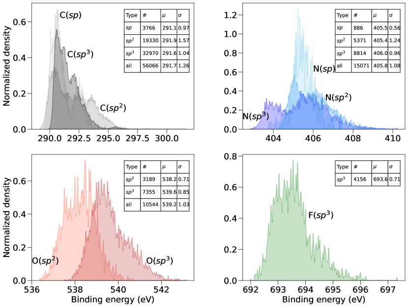
Figure 2: Normalized density plots of CEBEs for distinct hybridizations of CONF atoms in the bigQM7$\rm{\omega}$ dataset. ‘$\#$’ represents the number of entries, while mean, ‘$\mu$’ and standard deviation, ‘$\sigma$’ are presented in eV.

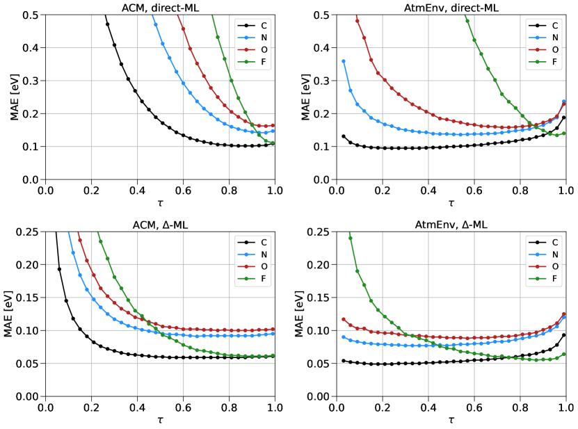
Figure 3: Variation of MAE (in eV) with $\tau$ for estimating the kernel width ($\sigma$), see Eq. 8 in the main text. Out-of-sample errors for predicting $E_{\rm b}^{1s}$ of C/N/O/F atoms in the bigQM7$\omega$ dataset are shown. Each point on a plot represents the out-of-sample error from an 80/20 train-test split. ACM denotes the atomic Coulomb matrix, while AtmEnv denotes the atomic environment determined from a graph neural network framework. The scheme direct-ML corresponds to learning on the target $E_{\rm b}^{1s}$ at the SCAN/Tight-Full level. For $\Delta-$ML, the target quantity is the difference: $E_{\rm b}^{\Delta-{\rm SCF}}{\rm(SCAN)}-E_{\rm b}^{\rm Koopmans}(\rm PBE@UFF)$; see the main text for more details. For each element, the cebeconf program uses $\tau$ corresponding to smallest MAE.

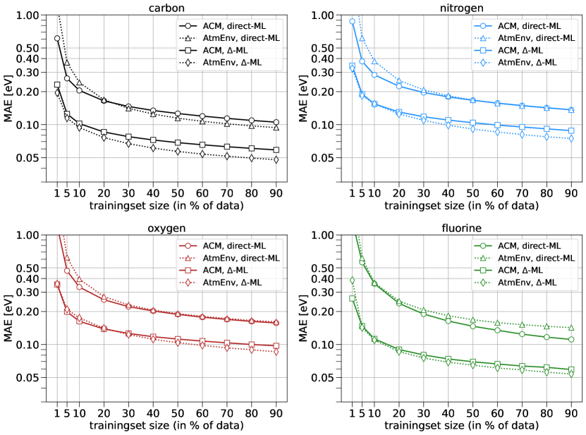
Figure 4: Learning curves showing out-of-sample errors for KRR-ML for predicting $E_{\rm b}^{1s}$ with increasing training set size. Results are shown separately for C, N, O, and F atoms. ACM and AtmEnv correspond to two variants of descriptors generated using UFF geometries. For direct-ML, the target quantity is 1$s$ CEBE determined using the SCAN/Tight-Full method within the $\Delta$-SCF formalism, while in $\Delta$-ML, the model is trained on the difference between the target and the baseline estimation of $E_{\rm b}^{1s}$ with in the Koopmans approximation determined with the PBE/cc-pVDZ method using UFF geometries.

Table 2: Prediction errors for the direct-ML and $\Delta$-ML models of $E_{\rm b}^{1s}$ for 208 uracil-type molecules depicted in FIG. 5. Errors are quantified with reference to the target values determined at the SCAN/Tight-Full level of theory within the $\Delta$-SCF formalism. The input for the ML models are structures determined using the universal force field (UFF). For $\Delta$-ML, additionally, 1$s$ energies of core-type molecular orbitals determined at the PBE/cc-pVDZ level using UFF geometries were used as the baseline. The mean absolute error (MAE) and the standard deviation (SD), shown in parentheses, are in eV. Pearson correlation coefficient, denoted by $R$, and the Spearman rank correlation coefficient, denoted by $\rho$, are also included. Error metrics are provided separately for carbon (C), nitrogen (N), oxygen (O), and fluorine (F) atoms within each set of molecules. The number of atoms of each type present in the set is included in the adjoining parentheses. The labels P2(1$H$), P4(1$H$), and P4(3$H$) correspond to Pyrimidine-2(1$H$)-one, Pyrimidine-4(1$H$)-one, and Pyrimidine-4(3$H$)-one, respectively.

Atom		Molecules		ML/ACM		$\Delta$-ML/ACM		ML/AtmEnv		$\Delta$-ML/AtmEnv
				MAE (SD), $R$, $\rho$		MAE (SD), $R$, $\rho$		MAE (SD), $R$, $\rho$		MAE (SD), $R$, $\rho$
C(72)		uracil		0.53 (0.53), 0.94, 0.95		0.35 (0.45), 0.96, 0.97		0.35 (0.28), 0.98, 0.98		0.20 (0.22), 0.99, 0.99
C(304)		P2(1$H$)		0.63 (0.64), 0.89, 0.90		0.38 (0.48), 0.94, 0.94		0.32 (0.35), 0.97, 0.97		0.25 (0.30), 0.98, 0.98
C(304)		P4(1$H$)		0.55 (0.61), 0.90, 0.90		0.39 (0.48), 0.94, 0.92		0.37 (0.47), 0.94, 0.93		0.22 (0.26), 0.98, 0.98
C(304)		P4(3$H$)		0.49 (0.58), 0.92, 0.92		0.30 (0.33), 0.97, 0.97		0.33 (0.43), 0.96, 0.96		0.12 (0.17), 0.99, 0.99
N(40)		uracil		0.39 (0.28), 0.81, 0.73		0.22 (0.16), 0.96, 0.96		0.48 (0.38), 0.74, 0.80		0.23 (0.23), 0.92, 0.90
N(176)		P2(1$H$)		0.45 (0.56), 0.90, 0.89		0.19 (0.22), 0.98, 0.98		0.47 (0.45), 0.93, 0.88		0.16 (0.20), 0.99, 0.99
N(176)		P4(1$H$)		0.46 (0.49), 0.95, 0.96		0.20 (0.25), 0.99, 0.99		0.57 (0.58), 0.89, 0.84		0.22 (0.28), 0.99, 0.99
N(176)		P4(3$H$)		0.39 (0.41), 0.90, 0.90		0.18 (0.20), 0.98, 0.98		0.76 (0.59), 0.84, 0.82		0.13 (0.16), 0.99, 0.99
O(32)		uracil		0.32 (0.33), 0.73, 0.73		0.21 (0.22), 0.95, 0.94		0.26 (0.24), 0.77, 0.74		0.09 (0.10), 0.96, 0.96
O(64)		P2(1$H$)		0.22 (0.30), 0.82, 0.82		0.24 (0.22), 0.94, 0.94		0.51 (0.45), 0.16, 0.12		0.15 (0.18), 0.89, 0.87
O(64)		P4(1$H$)		0.28 (0.25), 0.82, 0.79		0.33 (0.18), 0.96, 0.96		0.49 (0.34), 0.68, 0.66		0.25 (0.13), 0.94, 0.94
O(64)		P4(3$H$)		0.30 (0.38), 0.61, 0.56		0.20 (0.16), 0.96, 0.95		0.29 (0.31), 0.73, 0.71		0.08 (0.09), 0.98, 0.98
F(8)		uracil		0.40 (0.16), 0.97, 0.98		0.07 (0.07), 0.99, 1.00		0.47 (0.28), 0.95, 0.95		0.15 (0.14), 0.96, 1.00
F(48)		P2(1$H$)		0.35 (0.37), 0.72, 0.69		0.20 (0.09), 0.99, 0.98		0.40 (0.41), 0.79, 0.79		0.14 (0.16), 0.96, 0.97
F(48)		P4(1$H$)		0.25 (0.30), 0.83, 0.82		0.20 (0.12), 0.97, 0.98		0.45 (0.50), 0.62, 0.59		0.18 (0.19), 0.93, 0.93
F(48)		P4(3$H$)		0.32 (0.38), 0.71, 0.68		0.17 (0.12), 0.98, 0.98		0.53 (0.63), 0.10, 0.08		0.22 (0.21), 0.93, 0.93

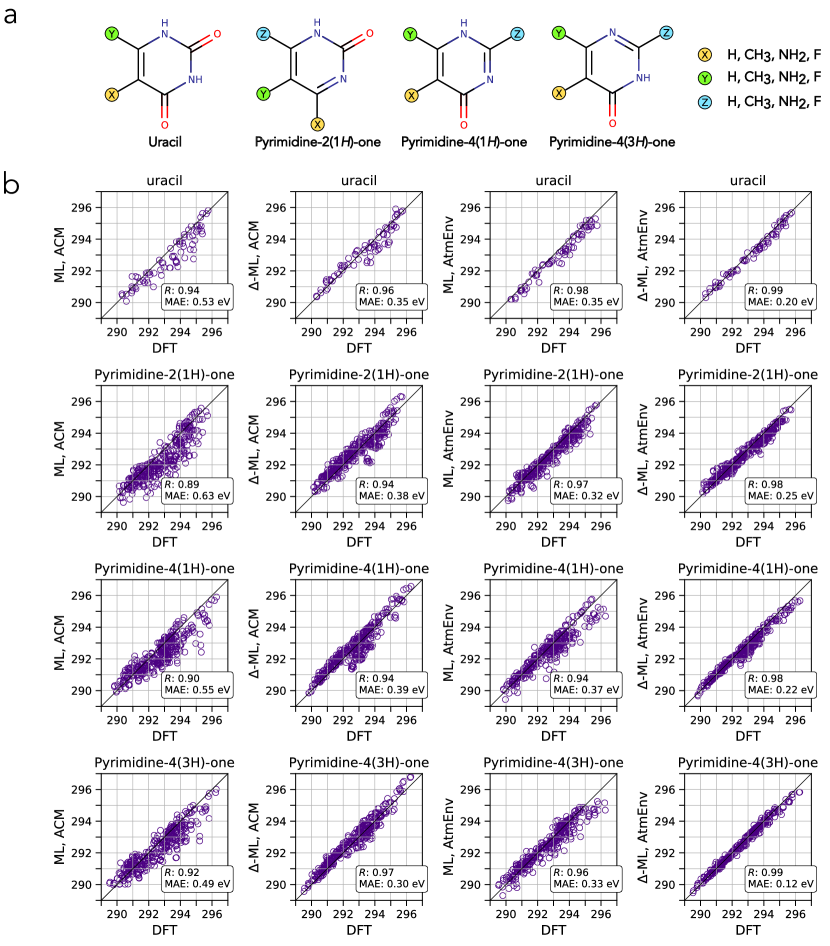
Figure 5: a.) Combinatorially varying set of biologically relevant molecules selected for validating the $E_{\rm b}^{1s}$ predicted by the ML models presented in this study. The number of derivatives are Uracil (Pyrimidine-2,4(1$H$,3$H$)-dione): 16, Pyrimidine-2(1$H$)-one: 64, Pyrimidine-4(1$H$)-one: 64, and Pyrimidine-4(3$H$)-one: 64, amounting to 208 unique molecules. b.) Scatterplot comparison of ML-predicted and DFT values of $E_{\rm b}^{1s}$ -C in 208 uracil derivatives. For all four classes of molecules, ML and $\Delta$-ML predictions are shown along with the Pearson correlation coefficient ($R$) and mean absolute error (MAE).

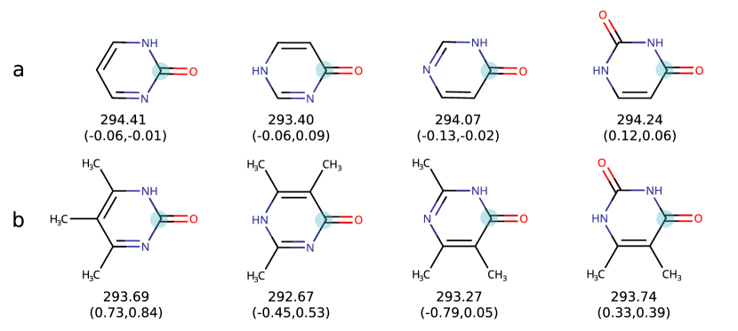
Figure 6: Effect of substitution of methyl groups (-CH₃) in the base molecules, shown in row-a, on the $E_{\rm b}^{1s}$ -C of the carbonyl group (blue circle). See the caption of FIG. 5a for the names of the molecules. Corresponding methylated molecules are shown in row-b. SCAN/Tight-Full, $\Delta$-SCF-based $E_{\rm b}^{1s}$ (in eV) of the C atom are given below each molecule. Error in predictions of direct-ML/AtmEnV and $\Delta$-ML/AtmEnv with respect to $\Delta$-SCF values are given in parenthesis.

III.2 Distribution of 1$s$-CEBEs of CONF atoms

For an atom in different molecular configurations, $E_{\rm b}^{1s}$ is influenced by a combination of the chemical environment provided by the neighboring atoms Greczynski and Hultman (2020) and screening effects Bagus, Ilton, and Nelin (2013). Normalized distributions of $E_{\rm b}^{1s}$ for different hybridizations of the CONF atoms in bigQM7$\rm{\omega}$ are shown in FIG. 2. The distribution is heavily biased towards $sp^{3}$-C with about thirty two thousand (32k) atoms, constituting about $38\%$ of 85k atoms in the dataset. Conversely, $sp$-N is the least represented, with only 886 atoms amounting to $0.01\%$ of the dataset. The challenge in assigning $E_{\rm b}^{1s}$ lies in the fact that these energies span narrow ranges with multiple chemical environments giving rise to identical values.

In the bigQM7$\rm{\omega}$ dataset, $E_{\rm b}^{1s}$ of F and C atoms have spreads of 0.71 and 1.26 eV, respectively (see FIG. 2). Separation into individual hybridizations does not decrease the spread of distribution. In some cases, the standard deviation worsens compared to the unseparated distribution. The high compositional diversity of the bigQM7$\rm{\omega}$ dataset renders substructure classification difficult due to the several unique connectivities possible for each atom type. We analyzed a subset of bigQM7$\rm{\omega}$ comprising 24 molecules with the unique substructure: $sp^{2}$-C bonded to N via a double bond, while bonded to O and F atoms through single bonds. See Figure S3 a) of the SI for the corresponding molecular structures. All molecules in the subset are 5-membered heterocyclic rings containing C, N, and O atoms that define the substructure. For the 25 F atoms in this molecular set, the distribution of $E_{\rm b}^{1s}$ span a range of 1.9 eV with a standard deviation of 0.5 eV, only 0.2 eV lower than that of all 4156 F atoms in the bigQM7$\rm{\omega}$ dataset. A comparison of the distributions is shown in Figure S3 b) of the SI. This indicates that partitioning $E_{\rm b}^{1s}$ of CONF atoms in bigQM7$\rm{\omega}$ based on substructure similarity does not decrease the spread of the values, and the scope for generating separate ML models based on substructure classification is limited.

III.3 Optimization of ML models

We probed the impact of the length of AtmEnv descriptor vector on the accuracy of KRR-ML models of $E_{\rm b}^{1s}$ of C atoms. Results, detailed in Table S3 of the SI, show that the out-of-sample prediction accuracy improves mariginally going from a length of 128 to 1024 for direct-ML predictions. Given an error of approximately 0.1 eV at length 128, the errors for lengths 32 and 64 are likely to exceed 0.1 eV. For $\Delta$-ML, the accuracy remains at 0.05 eV for length 128, slightly decreasing by only 7 meV at length 1024. Our goal of achieving an MAE below 0.1 eV for data-driven predictions of $E_{\rm b}^{1s}$ while keeping the computational complexity minimal led us to limit the length of AtmEnv to 128.

In order to visualize AtmEnv obtained from SchNet, we considered six classes of molecules not necessarily contained in bigQM7$\rm{\omega}$ : (a) CH₃-R, (b) CH₃-CH₂-R, (c) H₂C=C(H)-R, (d) HC$\equiv$C-R, (e) substituted benzene (C₆H₅-R), and (f) substituted cyclohexane (C₁₂H₁₁-R), where R = H, CH₃, NH₂, OH, and F. We used a trained SchNet model to generate AtmEnv for the ‘C’ atom marked and plotted the heatmaps shown in Figure S4 of the SI. The changes in the elements of AtmEnv with the groups bonded to C indicate how AtmEnv obtained from SchNet captures diverse atomic environments.

To determine the optimal kernel width, $\sigma_{\rm opt}$, for KRR-ML, we varied the parameter $\tau$ between 0 and 1 and applied Eq. 8. For each atom type, we used randomly selected 80% of the data to determine the hold out error on the remaining 20%. Further, we used same indices across different ML/descriptor combinations: direct-ML/ACM, direct-ML/AtmEnv, $\Delta$-ML/ACM, and $\Delta$-ML/AtmEnv. FIG. 3 displays the variation in MAE with $\tau$ for all atom types. $\Delta$-ML requires a smaller $\tau_{\rm opt}$ (hence larger $\sigma_{\rm opt}$ as per Eq. 8) than direct-ML for all atoms. This indicates the optimal kernel function for direct-ML to be broader, sampling over more training examples. The sensitivity of MAE to $\tau$ increases from C to F atoms. While $\sigma_{\rm opt}$ determined through scanning $\tau$ for $E_{\rm b}^{1s}$ -C are comparable to those determined using the heuristics proposed in a previous studyRamakrishnan and von Lilienfeld (2015) with $\tau=1/2$ (see Eq. 7), precise tuning becomes crucial for modeling $E_{\rm b}^{1s}$ of F. The optimal values of $\sigma_{\rm opt}$ determined using $\tau$ corresponding to the minimum MAE in FIG. 3 and Eq. 8 are hardcoded in the trained ML models provided in the module cebeconfTripathy et al. (2024).

III.4 Performance of ML models for out-of-sample predictions

FIG. 4 presents learning curves depicting the MAEs for out-of-sample prediction as a function of the training set size for various KRR-ML models. The monotonous drop in MAE with the training set implies that the models capture structure-property correlation that improve with increasing example data. Overall, across CONF elements, ACM and AtmEnv show similar learning trends for direct-ML predictions. While using 90% data of $E_{\rm b}^{1s}$ -C for training in direct and $\Delta$-ML, AtmEnv performs slightly better than ACM. Only in the case of direct-ML for $E_{\rm b}^{1s}$ -F, ACM converges to better accuracy than AtmEnv. Direct-ML predictions based on ACM and AtmEnv offer similar accuracies for N and O. In $\Delta$-ML, AtmEnv delivers consistently lower MAE compared to ACM for modeling 1$s$-CEBEs of all elements.

As discussed in III.2, $E_{\rm b}^{1s}$ of C is the most represented consisting of $\approx 65\%$ of the bigQM7$\rm{\omega}$ -CEBECONF dataset, achieving $\Delta$-ML MAE of 0.05 eV with AtmEnv descriptor. Additionally, the MAE for $E_{\rm b}^{1s}$ -F when using the $\geq 80\%$ of the data for training drops below 0.07 eV. However, a look at the distribution and composition of the F set offers insight into this high accuracy. Apart from the possibility of a single hybridization, all F atoms are connected to $sp^{3}$ C atoms, except the outliers HF and F₂, making the set compositionally more uniform compared to N and O. Hence, the distribution of $E_{\rm b}^{1s}$ -F also has a lower standard deviation compared to C/O/N, see 2. While N and O groups have a higher compositional diversity compared to F, their training sizes are not large compared to C, resulting in higher MAEs. Overall, for data-driven predictions of $E_{\rm b}^{1s}$ of C/O/N/F atoms to an accuracy of $\leq 0.1$ eV, $\Delta-$ML approach is necessary; the target accuracy is reached with 10%, 40%, 60%, and 20% of the data for C, N, O, and F atoms, respectively. Decreasing the error further may require better baselines in $\Delta$-ML or better geometries, both may incur additional expenses for out-of-sample predictions.

III.5 Transferability Test for ML models

Since $E_{\rm b}^{1s}$ is a property of an atom in a molecule, it is of interest to explore the transferability of the ML models trained on bigQM7$\rm{\omega}$ to new class of molecules. Hence, we have selected a set of aromatic heterocyclic systems as a validation set. Its composition is motivated by the potential application of the ML-models of $E_{\rm b}^{1s}$ to identify the composition of small biomolecules such as derivatives of nucleic acid bases, heavily substituted by O and N. Additionally, the use of substituted pyrimidines for synthesis is common Parker (2009). Particularly, up to two carbonyl groups have been included in pyrimidines generating derivatives of uracil, pyrimidine-2(1H)-one, pyrimidine-4(1H)-one and pyrimidine-4(3H)-one, see FIG. 5a. C atoms not attached to carbonyls are combinatorially substituted with either H, CH₃, NH₂ or F.

Each of the three pyrimidinones has a carbonyl group and three sites for substitution, leading to 64 derivatives in each class, summing to 192 molecules. Additionally, 16 substituted uracils are generated, since there are 2 carbonyls attached to a pyrimidine, availing the remaining 2 C atoms for substitution. These molecules contain 7-10 CONF atoms. The number of molecules containing 7,8,9 and 10, CONF atoms, are 1, 9, 27 and 27, respectively in each of the pyrimidinone sets. The uracil set has 1,6 and 9, molecules with 8,9, and 10 CONF atoms, respectively. Together, these 208 molecules constitute our validation set. Among them, only one (unsubstituted pyrimidine-2(1H)-one) is contained in bigQM7$\rm{\omega}$ . Along with this molecule, pyrimidine-4(1H)-one and pyrimidine-4(3H)-one are the only molecules in the validation set with 7 heavy atoms, while the rest are composed of more than 7 CONF atoms. Baseline energies for $\Delta$-ML are obtained at the same level of theory as in the training set, with aZORA corrected KS-eigenvalues obtained with the PBE/cc-pVDZ method using UFF-level molecular structures. One can also use the non-relativistic variant of these energies and correct them by adding 0.29/0.55/0.97/1.57 eV for C/O/N/F atoms, respectively. See Figure S1 for the details on these corrections.

ML-predicted CEBEs alongside DFT values are represented in scatter plots for all the ML models featured in FIG. 5b. Corresponding atom-specific errors for each class of molecules are tabulated in TABLE 2. Alike out-of-sample predictions in bigQM7$\rm{\omega}$ , discussed in III.4, the performance of direct-ML is inferior to that of $\Delta$-ML. Overall, all models, including direct-ML can achieve a high Pearson’s correlation coefficient, $R\approx 0.9$, for all classes of validation molecules. ACM models perform slightly worse, with direct-ML models based on ACM performing the poorest of all models, $\Delta$-ML/ACM has performance similar to direct-ML/AtmEnv predictions. $\Delta$-ML with AtmEnv shows the least errors, with $R\geq$ 0.98. In terms of element-specific accuracy, ACM has better prediction for N and F systems. Compared to explorations with the bigQM7$\rm{\omega}$ dataset, the accuracy of ML models has somewhat deteriorated while applying to large biomolecules. This is due to the fact that the molecules in the validation set are larger than those used for training the models. However, the qualitative trends between $E_{\rm b}^{1s}$ and the structural variations is captured by our ML models, indicated by the high correlation coefficients.

In FIG. 6, we compare ML-predicted $E_{\rm b}^{1s}$ with that of DFT values for the four unsubstituted bases shown in FIG. 5a and their CH₃ substituted counterpart shown in FIG. 5b. In particular, we explore the CEBEs of the C atom in a carbonyl group common to all four base molecules. Both direct-ML and $\Delta$-ML predictions show excellent accuracy for unsubstituted pyrimidine-2(1H)-one, which is contained in the bigQM7$\rm{\omega}$ dataset. For all four unsubstituted molecules, the $\Delta$-ML predictions show an error of $<0.1$ eV. Upon methylation, the CEBE at the carbonyl C decreases according to DFT predictions, while there is a drastic depreciation in the prediction accuracy of ML models. All predictions for the substituted molecules have errors above 0.3 eV except a single case of $\Delta$-ML prediction, where the the prediction is within an error of 0.05 eV. The same C with direct ML doesn’t show a similar drop in error, even though the training data is same for both direct-ML and $\Delta$-ML. Overall, this test of transferability of $\Delta$-ML/AtmEnv based on an inexpensive baseline suggests that CEBEs can be assigned to class of molecules with systematic variation of structure and composition with high degree of linear correlation. However, the models do not offer quantitative accuracy for the prediction of $E_{\rm b}^{1s}$ when the application is limited to a few molecules, as the models based on local descriptors do not capture long-range stereo-electronic effects resulting in accumulation of systematic errors.

IV Conclusion

In this study, we showcased the applicability of ML models for prediction of XPS. Using CEBEs determined using $\Delta$-SCF calculations, we generated the database, bigQM7$\rm{\omega}$ -CEBECONF, consisting of 12679 molecules from the bigQM7$\rm{\omega}$ dataset amounting to 85837 1$s$-CEBE of CONF atoms. For ML modeling, we explored the use of two descriptors: ACM, a local version of Coulomb matrix, and AtmEnv, a representation obtained from atom-specific embeddings of a graph neural network framework. KRR models were optimized by tuning the kernel widths determined specifically for each atomic model. The ML models reported in this study bypass the use of many body calculations or charge constraining algorithms, using only structural description of the molecule for predicting CEBEs. These models have been made accessible for general use through the python module cebeconfTripathy et al. (2024), where UFF level structures can be given as input to get CEBEs. The accuracy is leveraged further with the use of $\Delta$-ML using inexpensive baseline KS eigenvalues from single-point calculation on molecular geometry determined with force-fields.

For out-of-sample predictions within the bigQM7$\rm{\omega}$ dataset, $\Delta$-ML in combination with the AtmEnv descriptor offers an accuracy of less than 0.1 eV, which is an order of magnitude smaller than the spread of 1$s$-CEBE in the bigQM7$\rm{\omega}$ dataset. To understand the transferability of the models, we applied them to 208 biomolecules with homogeneously varying structure and compositions. Since these molecules are larger than the bigQM7$\rm{\omega}$ molecules used for training, their accuracy dropped compared to out-of-sample predictions within the bigQM7$\rm{\omega}$ dataset. However, they yield an overall correlation coefficient of over 0.9, suggesting that the prediction errors of the models is primely systematic, which can be calibrated using a few CEBEs determined at the target level.

V Supplementary material

See the supplementary material for the following: Figure S1 shows linear fits to obtain aZORA corrections for non-relativistic baseline energies. Figure S2 presents the choice of atomic indices in ACM representation on a schematic molecule. Figure S3 displays structures and normalized density plots for molecules with an identical substructure. Figure S4 shows the heatmaps of AtmEnv of ‘C’ atom in six classes of molecules. Table S1 shows the splitting of CEBEs in benzene. Table S2 gives the composition of the bigQM7$\rm{\omega}$ -CEBECONF dataset. Table S3 shows the variation of MAE for direct-ML and $\Delta$-ML with the length of AtmEnv. Table S4 provides the G_ΔHW₀ energies at cc-pVnZ and extrapolated values at CBS limit. The trained ML models are provided along with example validations at https://github.com/moldis-group/cebeconfTripathy et al. (2024).

VI Data Availability

The data that support the findings of this study are within the article and its supplementary material.

VII Acknowledgments

We thank Miguel Caro for providing the geometries of a subset of QM9 used in Ref. Golze et al., 2022. We thank Stijn De Baerdemacker for sharing the preprint of Ref. El-Samman et al., 2024b. ST thanks Dorothea Golze for commenting on questions regarding GW calculations. We thank Atreyee Majumder for assistance in calculations. We acknowledge the support of the Department of Atomic Energy, Government of India, under Project Identification No. RTI 4007. All calculations have been performed using the Helios computer cluster, which is an integral part of the MolDis Big Data facility, TIFR Hyderabad (http://moldis.tifrh.res.in).

VIII Author Declarations

VIII.1 Author contributions

ST: Conceptualization (equal); Analysis (equal); Data collection (main); Writing (equal). SD: Analysis (equal); Writing (equal). SJ: Analysis (equal); Writing (equal). RR: Conceptualization (equal); Analysis (equal); Funding acquisition; Project administration and supervision; Resources; Writing (equal).

VIII.2 Conflicts of Interest

The authors have no conflicts of interest to disclose.

References

References

- de Groot and Kotani (2008) F. de Groot and A. Kotani, Core Level Spectroscopy of Solids (CRC Press, 2008).
- Bagus, Sousa, and Illas (2022) P. S. Bagus, C. Sousa, and F. Illas, J. Phys.: Condens. Matter 34, 154004 (2022).
- Diller et al. (2014) K. Diller, F. Klappenberger, F. Allegretti, A. C. Papageorgiou, S. Fischer, D. A. Duncan, R. J. Maurer, J. A. Lloyd, S. C. Oh, K. Reuter, and J. V. Barth, J. Chem. Phys. 141, 144703 (2014).
- Ayiania et al. (2020) M. Ayiania, M. Smith, A. J. Hensley, L. Scudiero, J.-S. McEwen, and M. Garcia-Perez, Carbon 162, 528 (2020).
- Feng, Zhou, and Yang (2010) W. Feng, H. Zhou, and S.-z. Yang, Mater. Chem. Phys. 124, 287 (2010).
- Willmott (2019) P. Willmott, An introduction to synchrotron radiation: techniques and applications (John Wiley & Sons, 2019).
- Kovač et al. (2014) B. Kovač, I. Ljubić, A. Kivimäki, M. Coreno, and I. Novak, Phys. Chem. Chem. Phys. 16, 10734 (2014).
- Azuara-Tuexi, Muñoz-Sandoval, and Guirado-López (2023) G. Azuara-Tuexi, E. Muñoz-Sandoval, and R. Guirado-López, Phys. Chem. Chem. Phys. 25, 3718 (2023).
- Greczynski and Hultman (2020) G. Greczynski and L. Hultman, Prog. Mater. Sci. 107, 100591 (2020).
- Trinh et al. (2018) Q. T. Trinh, K. Bhola, P. N. Amaniampong, F. Jerome, and S. H. Mushrif, J. Phys. Chem. C 122, 22397 (2018).
- Nguyen et al. (2019) L. Nguyen, F. F. Tao, Y. Tang, J. Dou, and X.-J. Bao, Chem. Rev. 119, 6822 (2019).
- Yu et al. (2022) W. Yu, Z. Yu, Y. Cui, and Z. Bao, ACS Energy Lett. 7, 3270 (2022).
- Kohiki (1999) S. Kohiki, Spectrochim. Acta Part B At. Spectrosc. 54, 123 (1999).
- Chong, Gritsenko, and Baerends (2002) D. P. Chong, O. V. Gritsenko, and E. J. Baerends, J. Chem. Phys. 116, 1760 (2002).
- Bagus, Ilton, and Nelin (2013) P. S. Bagus, E. S. Ilton, and C. J. Nelin, Surf. Sci. Rep. 68, 273 (2013).
- Besley (2021) N. A. Besley, WIREs Comput. Mol. Sci. 11, e1527 (2021).
- Voora et al. (2019) V. K. Voora, R. Galhenage, J. C. Hemminger, and F. Furche, J. Chem. Phys. 151 (2019), 10.1063/1.5116908.
- Golze, Keller, and Rinke (2020) D. Golze, L. Keller, and P. Rinke, J. Phys. Chem. Lett. 11, 1840 (2020).
- Williams, DeGroot, and Sommers (1975) A. R. Williams, R. A. DeGroot, and C. B. Sommers, J. Chem. Phys. 63, 628 (1975).
- Jana and Herbert (2023) S. Jana and J. M. Herbert, J. Chem. Phys. 158 (2023), 10.1063/5.0134459.
- Bagus (1965) P. S. Bagus, Phys. Rev. 139, A619 (1965).
- Kahk and Lischner (2019) J. M. Kahk and J. Lischner, Phys. Rev. Mater. 3, 100801 (2019).
- Pueyo Bellafont, Viñes, and Illas (2016) N. Pueyo Bellafont, F. Viñes, and F. Illas, J. Chem. Theory Comput. 12, 324 (2016).
- Gilbert, Besley, and Gill (2008) A. T. B. Gilbert, N. A. Besley, and P. M. W. Gill, J. Phys. Chem. A 112, 13164 (2008).
- Carter-Fenk and Herbert (2020) K. Carter-Fenk and J. M. Herbert, J. Chem. Theory Comput. 16, 5067 (2020).
- Klein, Hall, and Maurer (2021) B. P. Klein, S. J. Hall, and R. J. Maurer, J. Phys.: Condens. Matter 33, 154005 (2021).
- Behler et al. (2007) J. Behler, B. Delley, K. Reuter, and M. Scheffler, Phys. Rev. B 75, 115409 (2007).
- Michelitsch and Reuter (2019) G. S. Michelitsch and K. Reuter, J. Chem. Phys. 150, 074104 (2019).
- Kayastha, Chakraborty, and Ramakrishnan (2022) P. Kayastha, S. Chakraborty, and R. Ramakrishnan, Digit. Discov. 1, 689 (2022).
- Tripathy et al. (2024) S. Tripathy, S. Das, S. Jindal, and R. Ramakrishnan, “cebeconf: A package of machine-learning models for predicting 1s-core electron binding energies of conf atoms in organic molecules.” (2024).
- Dorey et al. (2018) S. Dorey, F. Gaston, S. R. Marque, B. Bortolotti, and N. Dupuy, Appl. Surf. Sci. 427, 966 (2018).
- Ferraria, da Silva, and do Rego (2003) A. M. Ferraria, J. D. L. da Silva, and A. M. B. do Rego, Polymer 44, 7241 (2003).
- Ramakrishnan et al. (2014) R. Ramakrishnan, P. O. Dral, M. Rupp, and O. A. Von Lilienfeld, Sci. Data 1, 1 (2014).
- Rupp, Ramakrishnan, and Von Lilienfeld (2015) M. Rupp, R. Ramakrishnan, and O. A. Von Lilienfeld, J. Phys. Chem. Lett. 6, 3309 (2015).
- Ramakrishnan et al. (2015a) R. Ramakrishnan, P. O. Dral, M. Rupp, and O. A. Von Lilienfeld, J. Chem. Theory Comput. 11, 2087 (2015a).
- Gupta, Chakraborty, and Ramakrishnan (2021) A. Gupta, S. Chakraborty, and R. Ramakrishnan, Mach. learn.: sci. technol. 2, 035010 (2021).
- Watson et al. (2023) L. Watson, T. Pope, R. M. Jay, A. Banerjee, P. Wernet, and T. J. Penfold, Struct. Dyn. 10, 064101 (2023).
- Golze et al. (2022) D. Golze, M. Hirvensalo, P. Hernández-León, A. Aarva, J. Etula, T. Susi, P. Rinke, T. Laurila, and M. A. Caro, Chem. Mater. 34, 6240 (2022).
- Shiota, Ishihara, and Mizukami (2024) T. Shiota, K. Ishihara, and W. Mizukami, arXiv preprint arXiv:2402.18433 (2024), 10.48550/arXiv.2402.18433.
- El-Samman et al. (2024a) A. M. El-Samman, S. De Castro, B. Morton, and S. De Baerdemacker, Can. J. Chem. 102, 275 (2024a).
- El-Samman et al. (2024b) A. M. El-Samman, I. A. Husain, M. Huynh, S. De Castro, B. Morton, and S. De Baerdemacker, Digit. Discov. 3, 544 (2024b).
- Ramakrishnan et al. (2015b) R. Ramakrishnan, M. Hartmann, E. Tapavicza, and O. A. Von Lilienfeld, J. Chem. Phys. 143 (2015b), 10.1063/1.4928757.
- Gupta et al. (2021) A. Gupta, S. Chakraborty, D. Ghosh, and R. Ramakrishnan, J. Chem. Phys. 155 (2021), 10.1063/5.0076787.
- Fediai et al. (2023) A. Fediai, P. Reiser, J. E. O. Peña, W. Wenzel, and P. Friederich, Mach. learn.: sci. technol. 4, 035045 (2023).
- Ramakrishnan and von Lilienfeld (2017) R. Ramakrishnan and O. A. von Lilienfeld, Rev. Comput. Chem. 30, 225 (2017).
- Kotobi et al. (2023) A. Kotobi, K. Singh, D. Höche, S. Bari, R. H. Meißner, and A. Bande, J. Am. Chem. Soc. 145, 22584 (2023).
- Choudhury, Ramakrishnan, and Ghosh (2024) A. Choudhury, R. Ramakrishnan, and D. Ghosh, Chem. Commun. (2024).
- Aarva et al. (2019) A. Aarva, V. L. Deringer, S. Sainio, T. Laurila, and M. A. Caro, Chem. Mater. 31, 9243 (2019).
- Zarrouk et al. (2024) T. Zarrouk, R. Ibragimova, A. P. Bartók, and M. A. Caro, J. Am. Chem. Soc. (2024), 10.1021/jacs.4c01897.
- Chai and Head-Gordon (2008) J.-D. Chai and M. Head-Gordon, Phys. Chem. Chem. Phys. 10, 6615 (2008).
- Rappé et al. (1992) A. K. Rappé, C. J. Casewit, K. Colwell, W. A. Goddard III, and W. M. Skiff, J. Am. Chem. Soc. 114, 10024 (1992).
- Rupp et al. (2012) M. Rupp, A. Tkatchenko, K.-R. Müller, and O. A. von Lilienfeld, Phys. Rev. Lett. 108, 058301 (2012).
- Blum et al. (2009) V. Blum, R. Gehrke, F. Hanke, P. Havu, V. Havu, X. Ren, K. Reuter, and M. Scheffler, Comput. Phys. Comm. 180, 2175 (2009).
- Majumdar and Ramakrishnan (2024) A. Majumdar and R. Ramakrishnan, Phys. Chem. Chem. Phys. 26, 14505 (2024).
- Senthil, Chakraborty, and Ramakrishnan (2021) S. Senthil, S. Chakraborty, and R. Ramakrishnan, Chem. Sci. 12, 5566 (2021).
- Zhang et al. (2013) I. Y. Zhang, X. Ren, P. Rinke, V. Blum, and M. Scheffler, New J. Phys. 15, 123033 (2013).
- Sarangi et al. (2020) R. Sarangi, M. L. Vidal, S. Coriani, and A. I. Krylov, Mol. Phys. 118, e1769872 (2020).
- Mulliken (1955) R. S. Mulliken, J. Chem. Phys. 23, 1833 (1955).
- O’Boyle et al. (2011) N. M. O’Boyle, M. Banck, C. A. James, C. Morley, T. Vandermeersch, and G. R. Hutchison, J. Cheminform 3, 1 (2011).
- Bellafont, Bagus, and Illas (2015) N. P. Bellafont, P. S. Bagus, and F. Illas, J. Chem. Phys. 142 (2015), 10.1063/1.4921823.
- Li et al. (2022) J. Li, Y. Jin, P. Rinke, W. Yang, and D. Golze, J. Chem. Theory Comput. 18, 7570 (2022).
- Golze et al. (2018) D. Golze, J. Wilhelm, M. J. van Setten, and P. Rinke, J. Chem. Theory Comput. 14, 4856 (2018).
- Golze, Dvorak, and Rinke (2019) D. Golze, M. Dvorak, and P. Rinke, Front. Chem. 7, 377 (2019).
- Mejia-Rodriguez et al. (2022) D. Mejia-Rodriguez, A. Kunitsa, E. Aprà, and N. Govind, J. Chem. Theory Comput. 18, 4919 (2022).
- Frisch et al. (2016) M. J. Frisch, G. W. Trucks, H. B. Schlegel, G. E. Scuseria, M. A. Robb, J. R. Cheeseman, G. Scalmani, V. Barone, G. A. Petersson, H. Nakatsuji, X. Li, M. Caricato, A. V. Marenich, J. Bloino, B. G. Janesko, R. Gomperts, B. Mennucci, H. P. Hratchian, J. V. Ortiz, A. F. Izmaylov, J. L. Sonnenberg, D. Williams-Young, F. Ding, F. Lipparini, F. Egidi, J. Goings, B. Peng, A. Petrone, T. Henderson, D. Ranasinghe, V. G. Zakrzewski, J. Gao, N. Rega, G. Zheng, W. Liang, M. Hada, M. Ehara, K. Toyota, R. Fukuda, J. Hasegawa, M. Ishida, T. Nakajima, Y. Honda, O. Kitao, H. Nakai, T. Vreven, K. Throssell, J. A. Montgomery, Jr., J. E. Peralta, F. Ogliaro, M. J. Bearpark, J. J. Heyd, E. N. Brothers, K. N. Kudin, V. N. Staroverov, T. A. Keith, R. Kobayashi, J. Normand, K. Raghavachari, A. P. Rendell, J. C. Burant, S. S. Iyengar, J. Tomasi, M. Cossi, J. M. Millam, M. Klene, C. Adamo, R. Cammi, J. W. Ochterski, R. L. Martin, K. Morokuma, O. Farkas, J. B. Foresman, and D. J. Fox, “Gaussian˜16 Revision C.01,” (2016).
- van Lenthe, Snijders, and Baerends (1996) E. van Lenthe, J. G. Snijders, and E. J. Baerends, J. Chem. Phys. 105, 6505 (1996).
- Keller et al. (2020) L. Keller, V. Blum, P. Rinke, and D. Golze, J. Chem. Phys. 153, 114110 (2020).
- Kempgens et al. (1997) B. Kempgens, H. Köppel, A. Kivimäki, M. Neeb, L. Cederbaum, and A. Bradshaw, Phys. Rev. Lett. 79, 3617 (1997).
- Myrseth et al. (2002) V. Myrseth, K. Børve, K. Wiesner, M. Bässler, S. Svensson, and L. Sæthre, Phys. Chem. Chem. Phys. 4, 5937 (2002).
- Hergenhahn et al. (2001) U. Hergenhahn, O. Kugeler, A. Rüdel, E. E. Rennie, and A. M. Bradshaw, J. Phys. Chem. A 105, 5704 (2001).
- Matz, Nijssen, and Jagau (2023) F. Matz, J. Nijssen, and T.-C. Jagau, J. Phys. Chem. A 127, 6147 (2023).
- Hansen et al. (2015) K. Hansen, F. Biegler, R. Ramakrishnan, W. Pronobis, O. A. Von Lilienfeld, K.-R. Müller, and A. Tkatchenko, J. Phys. Chem. Lett. 6, 2326 (2015).
- Stuke et al. (2019) A. Stuke, M. Todorović, M. Rupp, C. Kunkel, K. Ghosh, L. Himanen, and P. Rinke, J. Chem. Phys. 150 (2019), 10.1063/1.5086105.
- Schölkopf et al. (2002) B. Schölkopf, A. J. Smola, F. Bach, et al., Learning with kt vector machines, regularization, optimization, and beyond (MIT press, 2002).
- Ramakrishnan and von Lilienfeld (2015) R. Ramakrishnan and O. A. von Lilienfeld, Chimia 69, 182 (2015).
- Behler and Parrinello (2007) J. Behler and M. Parrinello, Phys. Rev. Lett. 98, 146401 (2007).
- Szlachta, Bartók, and Csányi (2014) W. J. Szlachta, A. P. Bartók, and G. Csányi, Phys. Rev. B 90, 104108 (2014).
- Unke and Meuwly (2018) O. T. Unke and M. Meuwly, J. Chem. Phys. 148 (2018), 10.1063/1.5017898.
- Huang and von Lilienfeld (2020) B. Huang and O. A. von Lilienfeld, Nat. Chemistry 12, 945 (2020).
- Faber et al. (2018) F. A. Faber, A. S. Christensen, B. Huang, and O. A. Von Lilienfeld, J. Chem. Phys. 148 (2018), 10.1063/1.5020710.
- Von Lilienfeld (2013) O. A. Von Lilienfeld, Int. J. Quantum Chem. 113, 1676 (2013).
- Montavon et al. (2012) G. Montavon, K. Hansen, S. Fazli, M. Rupp, F. Biegler, A. Ziehe, A. Tkatchenko, A. Lilienfeld, and K.-R. Müller, Adv. Neural Inf. Process. Syst. 25 (2012).
- Hansen et al. (2013) K. Hansen, G. Montavon, F. Biegler, S. Fazli, M. Rupp, M. Scheffler, O. A. Von Lilienfeld, A. Tkatchenko, and K.-R. Müller, J. Chem. Theory Comput. 9, 3404 (2013).
- Jindal et al. (2022) S. Jindal, P.-J. Hsu, H. T. Phan, P.-K. Tsou, and J.-L. Kuo, Phys. Chem. Chem. Phys. 24, 27263 (2022).
- Schütt et al. (2018) K. Schütt, P. Kessel, M. Gastegger, K. Nicoli, A. Tkatchenko, and K. Müller, J. Chem. Theory Comput. 15, 448 (2018).
- Cho and Choi (2019) H. Cho and I. S. Choi, ChemMedChem 14, 1604 (2019).
- Te et al. (2018) G. Te, W. Hu, A. Zheng, and Z. Guo, in Proceedings of the 26th ACM international conference on Multimedia (2018) pp. 746–754.
- Mo et al. (2022) Y. Mo, L. Peng, J. Xu, X. Shi, and X. Zhu, in Proceedings of the AAAI Conference on Artificial Intelligence, Vol. 36 (2022) pp. 7797–7805.
- Hamilton, Ying, and Leskovec (2017) W. L. Hamilton, R. Ying, and J. Leskovec, arXiv preprint arXiv:1709.05584 (2017), 10.48550/arXiv.1709.05584.
- Kovács, Blaha, and Madsen (2023) P. Kovács, P. Blaha, and G. K. Madsen, J. Chem. Phys. 159 (2023), 10.1063/5.0179260.
- Ramakrishnan and Jain (2023) R. Ramakrishnan and S. Jain, J. Chem. Phys. 159 (2023), 10.1063/5.0166149.
- Parker (2009) W. B. Parker, Chem. Rev. 109, 2880 (2009).