Recurrent Deep Kernel Learning
of Dynamical Systems

Abstract

Digital twins require computationally-efficient reduced-order models (ROMs) that can accurately describe complex dynamics of physical assets. However, constructing ROMs from noisy high-dimensional data is challenging. In this work, we propose a data-driven, non-intrusive method that utilizes stochastic variational deep kernel learning (SVDKL) to discover low-dimensional latent spaces from data and a recurrent version of SVDKL for representing and predicting the evolution of latent dynamics. The proposed method is demonstrated with two challenging examples – a double pendulum and a reaction-diffusion system. Results show that our framework is capable of (i) denoising and reconstructing measurements, (ii) learning compact representations of system states, (iii) predicting system evolution in low-dimensional latent spaces, and (iv) quantifying modeling uncertainties.

Keywords Deep Kernel Learning  $\cdot$ Model-order Reduction  $\cdot$ Uncertainty Quantification

1 Introduction

A digital twin [1, 2, 3, 4] is a virtual replica that mimics the structure, context, and behaviour of a physical system. The digital twin is synchronized to its physical twin with data in real time to predict dynamical behaviours and inform critical decisions. Constructing a digital twin typically requires accurate modelling of complex physical phenomena that are often described by nonlinear, time-dependent, parametric partial differential equations (PDEs). Full-order models (FOMs) generated by detailed solvers are often computationally demanding and thus not suitable for the multi-query, real-time contexts in digital twinning, such as uncertainty quantification [5, 6, 7], optimal control [8, 9, 10], shape optimization [11], parameter estimation [12, 13], and model calibration [14, 15]. Therefore, constructing computationally efficient reduced-order models (ROMs) with controlled accuracy is crucial for dealing with real-world systems [16].

Generally speaking, any surrogate model that reduces the computational cost of a FOM can be considered a ROM. ROMs aim to intelligently represent high-dimensional dynamical systems in carefully-established low-dimensional latent spaces, so that the low-dimensionality improves computational efficiency, and the accuracy remains under control [17, 18, 19, 20, 21, 22, 16]. Despite the wide variety of approaches that can be found in the literature, we can identify two major categories of ROM approaches: intrusive and non-intrusive methods. Intrusive ROM techniques require access to the full-order solvers, which is often inconvenient in industrial implementations, especially for the cases involving legacy code and/or readily executed software. To overcome this limitation, non-intrusive ROM techniques have been developed to learn low-dimensional representations primarily from data, without accessing the code of FOMs. Such flexibility of non-intrusive ROMs has recently motivated the development of a vast amount of data-driven methods, such as dynamic mode decomposition [23, 24], reduced-order operator inference [25, 26, 27, 28], sparse identification of reduced latent dynamics [29, 30, 31, 32, 33, 34], manifold learning using deep auto-encoders [35, 36, 37, 38], data-driven approximation of time-integration schemes [39], and Gaussian process modeling for low-dimensional representations [40, 41].

However, learning ROMs from noisy data is extremely challenging. While many works in the literature have focused on learning compact representation of high-dimensional data, for example using neural networks (NNs) [42, 43], or quantifying uncertainties using, for example, Gaussian processes (GPs) [44], herein we argue that both challenges must be tackled simultaneously for discovering ROMs properly. NNs excel in learning complex and nonlinear dependencies of the data, while they tend to struggle when quantifying uncertainties. Conversely, GPs struggle with large dataset due to the limited expressivity of the kernels and the need for the inversion of the covariance matrix, while they excel to quantify uncertainties. To overcome these limitations, and to leverage on the positive features of both NNs and GPs synergistically, deep kernel learning (DKL) was introduced in recent years [45, 46]. DKL aims to combine the best of the GP and NN worlds by constructing a GP taking as input the data processed by a NN in order to learn expressive kernels that can model complex relations of the data.

In this paper, we exploit the DKL idea to develop a non-intrusive ROM that can deal with both high-dimensional and noisy data. In particular, with reference to Figure 1, our method includes a DKL encoder to compress high-dimensional measurements into low-dimensional distributions of state variables, a recurrent DKL latent dynamical model to predict the system’s evolution over time, and a decoder to reconstruct the measurements and interpret the latent representations.

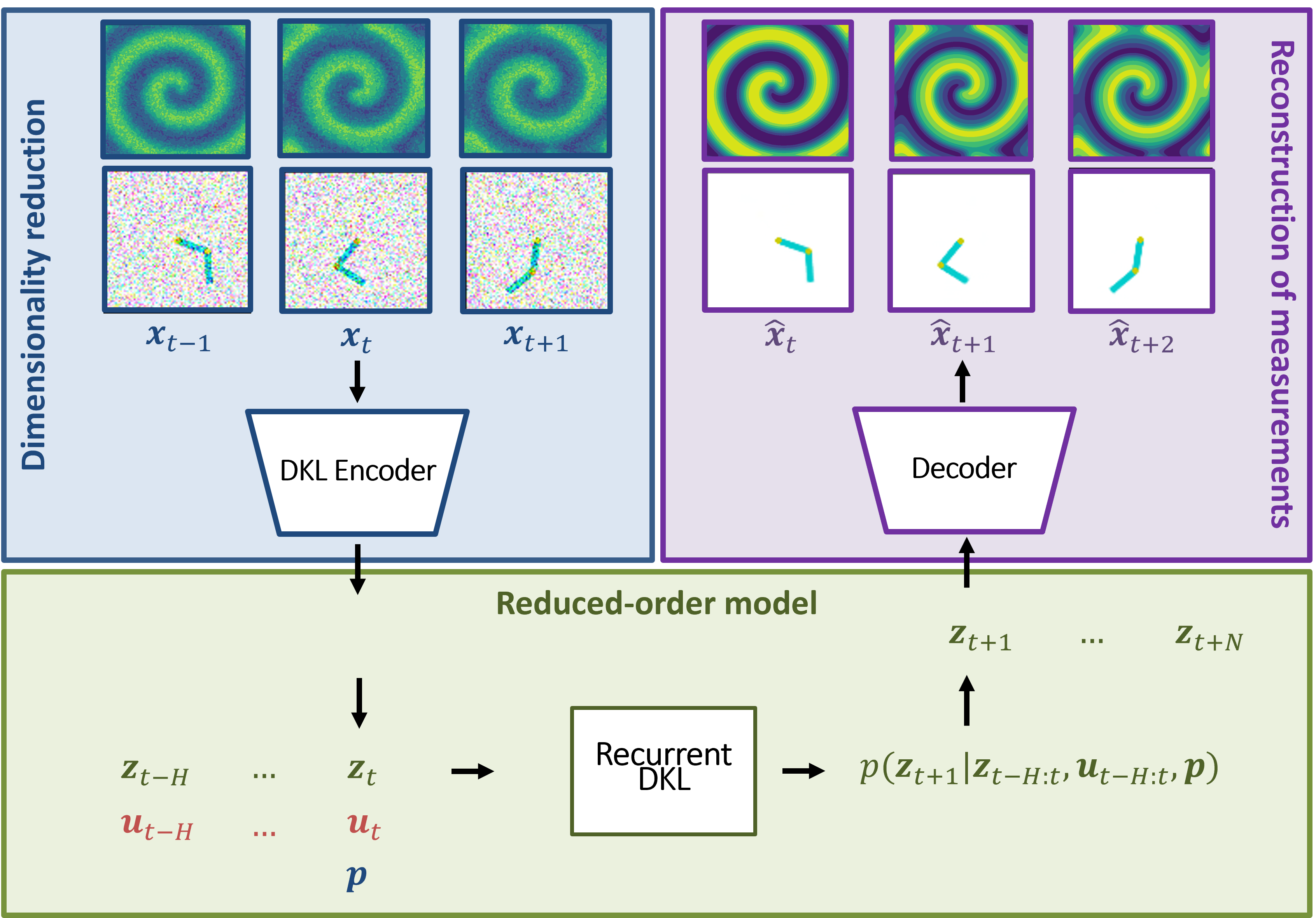
Figure 1: Proposed framework for reduced-order modelling of dynamical systems. We encode the measurements $\mathbf{x}_{t}$ at different time instances into the latent variables $\mathbf{z}_{t}$ by means of a deep kernel learning encoder. Then, we feed a sequence of length $H$ of consecutive latent variables $\mathbf{z}_{t-H:t}$, actions $\mathbf{u}_{t-H:t}$, and parameters $\mathbf{p}$ to a recurrent deep kernel learning to predict the next latent variable $\mathbf{z}_{t+1}$. The measurements are then reconstructed $\hat{\mathbf{x}}$ by means of a decoder from the latent variables.

The model is trained without labelled data in an unsupervised manner by only relying on high-dimensional and noisy measurements of the system. We show the capabilities of our framework in two challenging numerical examples, namely, the dynamics of (i) a double pendulum and of (ii) a distributed reaction-diffusion system, assuming in both cases to deal with measurements over a two-dimensional spatial region at different time instants – thus mimicking a set of observations acquired by a camera. Our contribution is threefold:

• we improve the prediction accuracy and consistency over long horizons of the DKL framework introduced in [41] by modelling the latent dynamics using a recurrent NN,

• we show the capabilities of the framework on challenging chaotic systems, i.e., a double pendulum and a reaction-diffusion problem, and

• we introduce an interpretable way for visualizing and studying uncertainties over latent variables by looking at the standard deviation in the measurement space.

The paper is organised as follows: in Section 2, we introduce the building blocks of our framework, namely GPs, and DKL, and in Section 3, we describe our novel DKL-based method. Section 4 presents the numerical experiments, shows and discusses the results, and Section 5 concludes the paper.

2 Preliminaries

Throughout this section, we assume to deal with a dataset of $N$ input vectors $X=[\mathbf{x}_{1},...,\mathbf{x}_{N}]$, in which the input is an element $\mathbf{x}\in\mathbb{R}^{|\mathbf{x}|}$ and $|\mathbf{x}|$ denotes its dimensionality, and correspondingly a vector of targets $\mathbf{y}=[y_{1},...,y_{N}]^{T}$, with the output $y\in\mathbb{R}$.

2.1 Gaussian Processes

A Gaussian process (GP) [44] $f(\mathbf{x})\sim\mathcal{GP}(\mu,k_{\boldsymbol{\gamma}})$ is a collection of random variables, any finite number of which is Gaussian distributed:

$$f(\mathbf{x})\sim\mathcal{GP}(\mu(\mathbf{x}),k(\mathbf{x},\mathbf{x}^{\prime};{\boldsymbol{\gamma}})),\ \ \ \ \ {y}=f(\mathbf{x})+\epsilon,\ \ \ \ \ \epsilon\sim\mathcal{N(}0,\sigma_{\epsilon}^{2})\,.$$ (1)

A GP is characterized by its mean function $\mu(\mathbf{x})=\mathbb{E}[f(\mathbf{x})]$ and its covariance/kernel function $k(\mathbf{x},\mathbf{x}^{\prime};{\boldsymbol{\gamma}})=k_{\boldsymbol{\gamma}}(\mathbf{x},\mathbf{x}^{\prime})=\mathbb{E}[(f(\mathbf{x})-\mu(\mathbf{x}))(f(\mathbf{x}^{\prime})-\mu(\mathbf{x}^{\prime}))]$ with hyperparameters $\boldsymbol{\gamma}$, $\mathbf{x}$ and $\mathbf{x}^{\prime}$ being two input locations, and $\epsilon$ is an additive noise term with variance $\sigma_{\epsilon}^{2}$. A popular choice of kernel is the squared-exponential (SE) kernel:

$$k_{{\boldsymbol{\gamma}}}(\mathbf{x},\mathbf{x}^{\prime})=\sigma_{f}^{2}\exp\left(-\frac{1}{2}\frac{||\mathbf{x}-\mathbf{x}^{\prime}||^{2}}{l^{2}}\right)\,,$$ (2)

with $\boldsymbol{\gamma}=[\sigma_{f}^{2},l]$, $\sigma_{f}^{2}$ being a noise scale and $l$ the length scale. The hyperparameters of the GP regression, namely $[\boldsymbol{\gamma},\sigma_{\epsilon}^{2}]$, can be estimated by maximizing the marginal likelihood as follows:

$$\begin{split}[\boldsymbol{\gamma}^{*},(\sigma_{\epsilon}^{2})^{*}]&=\arg\max_{\boldsymbol{\gamma},\sigma_{\epsilon}^{2}}\leavevmode\nobreak\ \log p(\mathbf{y}|X)\\ &=\arg\max_{\boldsymbol{\gamma},\sigma_{\epsilon}^{2}}\left\{-\frac{1}{2}\mathbf{y}^{T}(k_{\boldsymbol{\gamma}}(X,X)+\sigma_{\epsilon}^{2}I)^{-1}\mathbf{y}-\frac{1}{2}\log|k_{\boldsymbol{\gamma}}(X,X)+\sigma_{\epsilon}^{2}I|-\frac{N}{2}\log(2\pi)\right\}\,,\\ \end{split}$$ (3)

Given the training data of input-output pairs $(X,\mathbf{y})$, the standard rule for conditioning Gaussians gives a predictive (posterior) Gaussian distribution of the noise-free outputs $\mathbf{f}^{*}$ at unseen test inputs ${X}^{*}$:

$$\begin{split}\mathbf{f}^{*}|X^{*},X,\mathbf{y}&\sim\mathcal{N}(\boldsymbol{\mu}^{*},\Sigma^{*})\,,\\ \boldsymbol{\mu}^{*}&=k_{\boldsymbol{\gamma}}(X,X^{*})^{T}(k_{\boldsymbol{\gamma}}(X,X)+\sigma_{\epsilon}^{2}I)^{-1}(\mathbf{y}-\mu(X))\,,\\ \Sigma^{*}&=k_{\boldsymbol{\gamma}}(X^{*},X^{*})-k_{\boldsymbol{\gamma}}(X,X^{*})^{T}(k_{\boldsymbol{\gamma}}(X,X)+\sigma_{\epsilon}^{2}I)^{-1}k_{\boldsymbol{\gamma}}(X,X^{*})\,.\\ \end{split}$$ (4)

2.2 Deep Kernel Learning

The choice of the kernel is a crucial aspect for the performance of a GP. For example, a SE kernel (see Equation 2) can only learn information about the data using the noise-scale and the length-scale parameters, which tell us how quickly the correlation in our data varies with respect to the distance of the input-data pairs. This is clearly a limiting factor when dealing with complex datasets with non-trivial dependencies and correlations. To overcome the problem of the limited expressivity of GP kernels, deep kernel learning (DKL) was introduced in [44].

The key idea of DKL is to embed a (deep) NN $g(\mathbf{x};\boldsymbol{\theta})$ of parameters $\boldsymbol{\theta}$, i.e., the weights and biases of the NN, into the kernel function of a GP:

$$k_{\text{DKL}}(\mathbf{x},\mathbf{x^{\prime}};{\boldsymbol{\gamma}},\boldsymbol{\theta})=k_{{\boldsymbol{\gamma}}}(g(\mathbf{x};\boldsymbol{\theta}),g(\mathbf{x^{\prime}};\boldsymbol{\theta}))=k(g(\mathbf{x};\boldsymbol{\theta}),g(\mathbf{x^{\prime}};\boldsymbol{\theta});\boldsymbol{\gamma})\,.$$ (5)

In this way, we can rely on the expressive power of NNs to learn compact and low-dimensional representations of the data, and unveil the non-trivial dependencies of the data. Then, we can feed these representations to the GP for quantifying the uncertainties.

The GP hyperparameters $\boldsymbol{\gamma}$ and the NN paramameters $\boldsymbol{\theta}$ are jointly learned by maximizing the log marginal likelihood (see Equation (3)). It is possible to use the chain rule to compute derivatives of the log marginal likelihood, that we indicate with $\mathcal{L}(\boldsymbol{\gamma},\boldsymbol{\theta})$, with respect to kernel hyperparameters $\boldsymbol{\gamma}$ and the NN parameters $\boldsymbol{\theta}$, thus obtaining:

$$\frac{\partial\mathcal{L}(\boldsymbol{\gamma},\boldsymbol{\theta})}{\partial{\boldsymbol{\gamma}}}=\frac{\partial\mathcal{L}(\boldsymbol{\gamma},\boldsymbol{\theta})}{\partial k_{{\boldsymbol{\gamma}}}}\frac{\partial k_{{\boldsymbol{\gamma}}}}{\partial{\boldsymbol{\gamma}}},\hskip 19.91684pt\frac{\partial\mathcal{L}(\boldsymbol{\gamma},\boldsymbol{\theta})}{\partial\boldsymbol{\theta}}=\frac{\partial\mathcal{L}(\boldsymbol{\gamma},\boldsymbol{\theta})}{\partial k_{{\boldsymbol{\gamma}}}}\frac{\partial k_{{\boldsymbol{\gamma}}}}{\partial g(\mathbf{x},\boldsymbol{\theta})}\frac{\partial g(\mathbf{x},\boldsymbol{\theta})}{\partial\boldsymbol{\theta}}.$$ (6)

Optimizing the GP hyperparameters through Equation (3) requires to repeatedly invert the covariance matrix $k_{\boldsymbol{\gamma}}(X,X)+\sigma_{\epsilon}^{2}I$, with size $N\times N$. However, for large datasets, i.e., when $N\gg 1$, the full covariance matrix may be too large to be stored in memory and inverted. In these cases, it is common practice in machine learning to utilize minibatches of randomly-samples data points to compute the loss functions and compute the gradients. However, when we use minibatches to train the GPs, the posterior distribution is not Gaussian anymore, even when a Gaussian likelihood is used. When dealing with non-Gaussian posteriors, we can rely on variational inference (VI) [47]. VI is an approximation technique for dealing with non-Gaussian posteriors, deriving from minibatch training and/or non-Gaussian likelihoods. VI allows one to approximate the posterior by the best-fitting Gaussian distribution using a set of samples, often called inducing points, from the posterior.

Stochastic variational DKL (SVDKL) [46] extends DKL to minibatch training and non-Gaussian posteriors by means of VI. SVDKL can deal with large dataset, effectively mitigating the main limitations of traditional GPs. SVDKL is also considerably cheaper than Bayesian NNs or ensembles methods [48, 49], making it an essential architecture in many applications. SVDKL can be used as a building block for learning ROMs from high-dimensional and noisy data [41]. The framework proposed in [41] is composed of (i) a SVDKL encoder-decoder scheme for learning low-dimensional representations of the data and (ii) a SVDKL using the representations to predict the dynamics of the systems forward in time. The encoder-decoder scheme resembles a variational autoencoder [50], but with better uncertainty quantification capabilities due to the presence of the GP kernel.

3 Recurrent Stochastic Variational Deep Kernel Learning for Dynamical Systems

3.1 Problem Statement

In our research, we consider nonlinear dynamical systems expressed in the state-space form:

$$\dot{\mathbf{s}}(t)=f(\mathbf{s}(t),\mathbf{u}(t);\mathbf{p}),\hskip 14.22636pt\mathbf{s}(t_{0})=\mathbf{s}_{0},\hskip 14.22636ptt\in[t_{0},t_{f}]\,,$$ (7)

where $\mathbf{s}(t)\in\mathbb{R}^{|\mathbf{s}|}$ represents the state vector at time $t$, $\dot{\mathbf{s}}(t)$ its time derivative, $\mathbf{u}(t)\in\mathbb{R}^{|\mathbf{u}|}$ is the control input at time $t$, $\mathbf{p}\in\mathbb{R}^{|\mathbf{p}|}$ is the vector of parameters, $\mathbf{s}_{0}$ is the initial condition, and $t_{0}$ and $t_{f}$ are the initial and final times, respectively. The nonlinear function $f$ determines the evolution of the system with respect to the current state $\mathbf{s}(t)$ and control input $\mathbf{u}(t)$.

In many real-world applications, the state $\mathbf{s}(t)$ and the FOM $f$ may be unknown or not readily available. However, we can often obtain indirect information about these systems through measurements collected by sensor devices. We denote the measurements at a generic timestep $t$ with $\mathbf{x}_{t}$, with $\mathbf{x}\in\mathbb{R}^{|\mathbf{x}|}$, and the measurement at timestep $t+1$ as $\mathbf{x}_{t+1}$ due to the discrete-time nature of the measurements. Given a set of $M$ observed trajectories $\Xi=[X_{1},\cdots,X_{M}]$, controls $\Omega=[U_{1},\cdots,U_{M}]$, and parameters $P=[\mathbf{p}_{1},\cdots,\mathbf{p}_{M}]$, if any, where for each trajectory we collect $N$ high-dimensional and noisy measurements $X_{i}=[\mathbf{x}_{1},\cdots,\mathbf{x}_{N}]$, $N-1$ control inputs $U_{i}=[\mathbf{u}_{1},\cdots,\mathbf{u}_{N-1}]$, and one parameter vector $\mathbf{p}_{i}$, our objective is to introduce a framework for: (i) learning a compact representation $\mathbf{z}$ of the unknown state variables $\mathbf{s}$, and (ii) learning a surrogate ROM $\xi$ as a proxy for $f$ that predicts the dynamics of the latent state variables, given, if any, control inputs and parameters. Due to the high dimensionality and corruption of the measurement data, and the unsupervised nature of the learning process, achieving objectives (i) and (ii) is extremely challenging.

3.2 Model Architecture

To tackle these two challenges, we introduce a novel recurrent SVDKL architecture (see Figure 1) that is composed of three main blocks (see Figure 2, 3, and 4, respectively):

1. an SVDKL encoder that projects the high-dimensional measurements $\mathbf{x}$ into a Gaussian distribution over the latent state variables $p(\mathbf{z}|\mathbf{x})$,

2. a decoder that reconstructs the measurements $\hat{\mathbf{x}}$ from the latent variables $\mathbf{z}$, and

3. a recurrent SVDKL forward dynamical model predicting the evolution of the system using a history of latent state variables $\mathbf{z}_{t-H},\cdots,\mathbf{z}_{t}$ and control inputs $\mathbf{u}_{t-H},\cdots,\mathbf{u}_{t}$, and parameters $\mathbf{p}$, if available.

With reference to Figure 2, the encoder $\phi:\mathbb{R}^{|\mathbf{x}|}\rightarrow[0,1]^{|\mathbf{z}|}$ is modeled using a SVDKL of parameters $\boldsymbol{\theta}_{\phi}$ and hyperparameters $\boldsymbol{\gamma}_{\phi},\sigma_{\phi}^{2}$, with $[0,1]^{|\mathbf{z}|}$ indicating the distribution over the latent variables $\mathbf{z}$. In particular, the encoder $\phi$ maps a high-dimensional measurement $\mathbf{x}_{t}$ to a latent state distribution $p(\mathbf{z}_{t}|\mathbf{x}_{t})$:

$$\begin{split}z_{i,t}&=f_{i}^{\phi}(\mathbf{x}_{t})+\epsilon_{\phi},\quad\epsilon_{\phi}\sim\mathcal{N}(0,\sigma^{2}_{\phi})\,,\\ f_{i}^{\phi}(\mathbf{x}_{t})&\sim\mathcal{GP}(\mu(g_{\phi}(\mathbf{x}_{t};\boldsymbol{\theta}_{\phi})),k(g_{\phi}(\mathbf{x}_{t};\boldsymbol{\theta}_{\phi}),g_{\phi}(\mathbf{x}^{\prime}_{t^{\prime}};\boldsymbol{\theta}_{\phi});\boldsymbol{\gamma}_{\phi,i})),\quad 1\leq i\leq|\mathbf{z}|\,,\end{split}$$ (8)

where $z_{i,t}$ indicates the sample from the $i^{th}$ GP with SE kernel $k(\bullet,\bullet^{\prime};\boldsymbol{\gamma}_{\phi})$ and mean $\mu$, $\epsilon_{\phi}$ is an independently-added noise, and $|\mathbf{z}|$ indicates the dimension of $\mathbf{z}$. The GP inputs $g_{\phi}(\mathbf{x}_{t};\boldsymbol{\theta}_{\phi})$ and $g_{\phi}(\mathbf{x}^{\prime}_{t};\boldsymbol{\theta}_{\phi})$ are the representations of the data pair $(\mathbf{x},\mathbf{x}^{\prime})$ obtained from the NN $g_{\phi}(\bullet;\boldsymbol{\theta}_{\phi})$ with parameters $\boldsymbol{\theta}_{\phi}$.

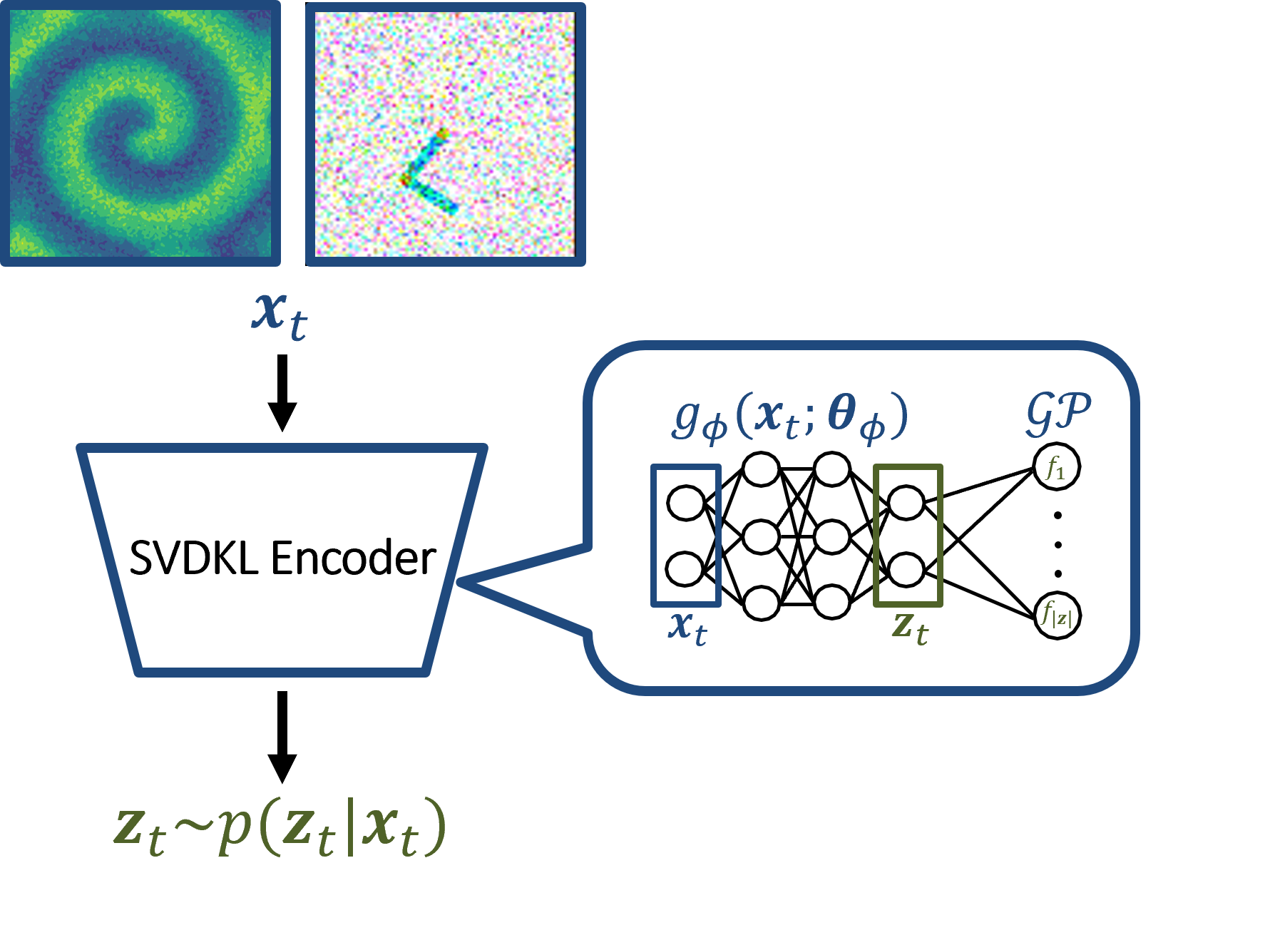
Figure 2: Architecture of the SVDKL encoder.

With reference to Figure 3, the decoder $\psi$ is modeled using an NN with parameters $\boldsymbol{\theta}_{\psi}$. The decoder maps a sample $\mathbf{z}$ to the conditional distribution $p(\hat{\mathbf{x}}|\mathbf{z})$. Similar to VAEs [50], the distribution $p(\hat{\mathbf{x}}|\mathbf{z})$ is approximated to be independently distributed Gaussian distributions. In general, the decoding NN $\psi$ learns the means and variances of these distributions. Following [51, 52], however, our decoder in this work only learns the mean vector of $\hat{\mathbf{x}}|\mathbf{z}$, while the covariance is set to the identity matrix $I$, i.e., $\psi:\mathbb{R}^{|\mathbf{z}|}\rightarrow[0,1]^{|\mathbf{x}|}$ and

$$\hat{\mathbf{x}}_{t}|\mathbf{z}_{t}\sim\mathcal{N}\psi(\mathbf{z}_{t};\boldsymbol{\theta}_{\psi}),I).$$ (9)

The reconstruction $\hat{\mathbf{x}}_{t}$ can be obtained by feeding $\mathbf{z}_{t}$ to the decoder $\psi$ and then sampling from this distribution.

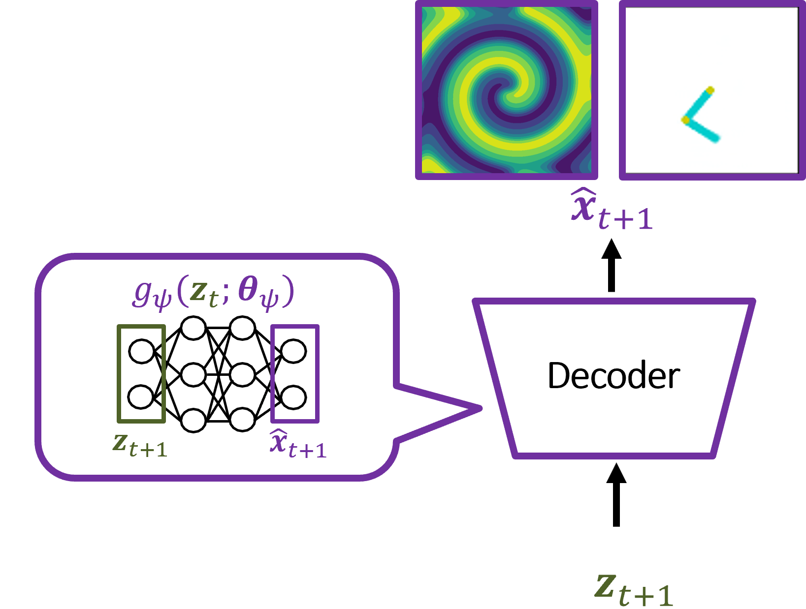
Figure 3: Architecture of the decoder.

With reference to Figure 4, the forward dynamical model $\xi:\mathbb{R}^{|\mathbf{z}|}\times\mathbb{R}^{|\mathbf{u}|}\times\mathbb{R}^{|\mathbf{p}|}\rightarrow[0,1]^{|\mathbf{z}|}$, with parameters $\boldsymbol{\theta}_{\xi}$ and hyperparameters $\boldsymbol{\gamma}_{\xi},\sigma_{\xi}^{2}$, is a SVDKL with a recurrent NN architecture, i.e., a long short-term memory (LSTM) NN [53], that maps sequences of latent states, actions, and parameters to latent next state distribution $p(\mathbf{z}_{t+1}|\mathbf{z}_{t-H:t},\mathbf{u}_{t-H:t},\mathbf{p})$. In particular, we can write the latent next states $\mathbf{z}_{t+1}$ as:

$$\begin{split}z_{i,t+1}&=f_{i}^{\xi}(\mathbf{z}_{t-H:t},\mathbf{u}_{t-H:t},\mathbf{p})+\epsilon_{\xi},\quad\epsilon_{\xi}\sim\mathcal{N}(0,\sigma^{2}_{\xi})\,,\\ f_{i}^{\xi}(\bullet)&\sim\mathcal{GP}(\mu(g_{\xi}(\bullet;\boldsymbol{\theta}_{\xi}),k(g_{\xi}(\bullet;\boldsymbol{\theta}_{\xi}),g_{\xi}(\bullet^{\prime};\boldsymbol{\theta}_{\xi});\boldsymbol{\gamma}_{{\xi},i}))\,,\quad 1\leq i\leq|\mathbf{z}|\,,\end{split}$$ (10)

where $z_{i,t+1}$ is sampled from the $i^{th}$ GP, $H$ is the history length, and $\epsilon_{\xi}$ is a noise term. Similarly to the encoder, the GP inputs $g_{\xi}(\mathbf{z}_{t-H:t},\mathbf{u}_{t-H:t},\mathbf{p};\boldsymbol{\theta}_{\xi})$ and $g_{\xi}(\mathbf{z}^{\prime}_{t-H:t},\mathbf{u}^{\prime}_{t-H:t},\mathbf{p}^{\prime};\boldsymbol{\theta}_{\xi})$ are the representations of obtained from the NN $g_{\xi}(\bullet;\boldsymbol{\theta}_{\xi})$ with parameters $\boldsymbol{\theta}_{\xi}$.

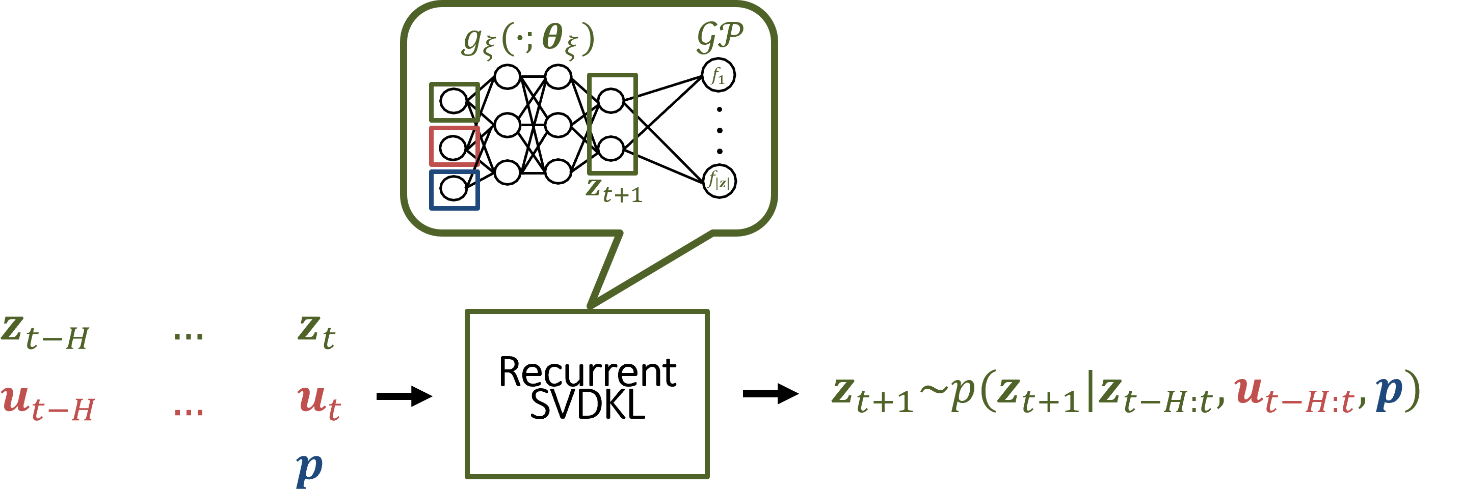
Figure 4: Architecture of the forward dynamical model.

The encoder and decoder have the same NN architecture proposed in [41]. On the other hand, the forward dynamical model replaces the fully-connected NN used in [41] with a recurrent neural network to improve the reliability and accuracy of the predictions forward in time.

3.3 Training Objectives

The aforementioned encoder, decoder, and forward dynamical model are jointly trained to infer meaningful low-dimensional representations of the measurements and predict the system evolution forward in time. The first objective term is formulated by utilizing the reconstruction loss, commonly used for training VAEs, which maximizes the marginal likelihood for the reconstruction of ${\mathbf{x}}_{t}$ by $\hat{\mathbf{x}}_{t}$:

$$\mathcal{L}_{\text{recon}}(\boldsymbol{\theta}_{\phi},\boldsymbol{\gamma}_{\phi},\sigma^{2}_{\phi},\boldsymbol{\theta}_{\psi})=\mathbb{E}_{\mathbf{x}_{t}\sim\Xi}[-\log\mathbb{E}_{{\mathbf{z}}_{t}|\mathbf{x}_{t}}p(\hat{\mathbf{x}}_{t}|\mathbf{z}_{t})]\,,$$ (11)

where $\hat{\mathbf{x}}_{t}$ is the reconstructed vector of the measurement $\mathbf{x}_{t}$, obtained by feeding $\mathbf{x}_{t}$ through the encoder $\phi$ and decoder $\psi$, $p(\mathbf{z}|\mathbf{x})$ is the distribution learned by the encoder (see Equation (8)), and $p(\hat{\mathbf{x}}|\mathbf{z})$ the distribution learned by the decoder (see Equation (9)). The minimization of loss function in Equation (11) with respect to the encoder and decoder parameters is analogous to the one commonly used by VAEs, which allows us to learn compact representations of the measurements while quantifying the uncertainties in the reconstructions.

For training the dynamical model $\xi$, we do not rely on true state values $\mathbf{s}$, but on the sequences of measurements collected at different time steps $t$. Therefore, we are not able to use supervised learning techniques to optimize the NN parameters and kernel hyperparameters. However, we can use the posterior distribution $p(\mathbf{z}_{t+1}|\mathbf{x}_{t+1})$ (see Equation (8)) as the target distribution for learning $p(\mathbf{z}_{t+1}|\mathbf{z}_{t-H:t},\mathbf{u}_{t-H:t},\mathbf{p})$. This process translates into evaluating the Kullback-Leiber (KL) divergence between these two distributions:

$$\begin{split}&\mathcal{R}_{\text{reg}}^{(1)}(\boldsymbol{\theta}_{\phi},\boldsymbol{\gamma}_{\phi},\sigma^{2}_{\phi},\boldsymbol{\theta}_{\psi},\boldsymbol{\theta}_{\xi},\boldsymbol{\gamma}_{\xi},\sigma^{2}_{\xi})\\ =\leavevmode\nobreak\ &\text{KL}\left[p(\mathbf{z}_{t+1}|\mathbf{x}_{t+1})||\mathbb{E}_{\mathbf{z}_{t-H:t}|\mathbf{x}_{t-H:t}}p(\mathbf{z}_{t+1}|\mathbf{z}_{t-H:t},\mathbf{u}_{t-H:t},\mathbf{p})\right]\,,\end{split}$$ (12)

where the superscript $(1)$ in $\mathcal{R}_{\text{reg}}^{(1)}$ indicates that we perform a 1-step ahead prediction of the latent states from time step $t$ to $t+1$. The distribution $p(\mathbf{z}_{t+1}|\mathbf{x}_{t+1})$ is obtained by encoding the next measurement $\mathbf{x}_{t+1}$ through $\phi$ (see Figure 2), $p(\mathbf{z}_{t+1}|\mathbf{z}_{t-H:t},\mathbf{u}_{t-H:t},\mathbf{p})$ is the distribution obtained by the forward dynamical model $\xi$ (see Figure 4), and the expectation $\mathbb{E}_{\mathbf{z}_{t-H:t}|\mathbf{x}_{t-H:t}}$ indicates the marginalization of a sequence of latent variables $\mathbf{z}_{t-H:t}$ obtained by feeding the measurements $\mathbf{x}_{t-H:t}$ to the encoder $\phi$. Different from [41], we extend this loss to $T$-step predictions:

$$\mathcal{L}_{\text{reg}}(\boldsymbol{\theta}_{\phi},\boldsymbol{\gamma}_{\phi},\sigma^{2}_{\phi},\boldsymbol{\theta}_{\psi},\boldsymbol{\theta}_{\xi},\boldsymbol{\gamma}_{\xi},\sigma^{2}_{\xi})=\mathbb{E}_{\mathbf{x}\sim\Xi,\mathbf{u}\sim\Omega,\mathbf{p}\sim P}\frac{1}{T}\sum_{i=1}^{T}\mathcal{R}_{\text{reg}}^{(i)}(\boldsymbol{\theta}_{\phi},\boldsymbol{\gamma}_{\phi},\sigma^{2}_{\phi},\boldsymbol{\theta}_{\psi},\boldsymbol{\theta}_{\xi},\boldsymbol{\gamma}_{\xi},\sigma^{2}_{\xi})\,,$$ (13)

where we now perform $T$-step ahead predictions from time step $t+1$ to $t+T$, and

$$\begin{split}&\mathcal{R}_{\text{reg}}^{(i)}(\boldsymbol{\theta}_{\phi},\boldsymbol{\gamma}_{\phi},\sigma^{2}_{\phi},\boldsymbol{\theta}_{\psi},\boldsymbol{\theta}_{\xi},\boldsymbol{\gamma}_{\xi},\sigma^{2}_{\xi})\\ =\leavevmode\nobreak\ &\text{KL}\left[p(\mathbf{z}_{t+i}|\mathbf{x}_{t+i})||\mathbb{E}_{\mathbf{z}_{t+i-1-H:t+i-1}|\mathbf{x}_{t+i-1-H:t+i-1}}p(\mathbf{z}_{t+i}|\mathbf{z}_{t+i-1-H:t+i-1},\mathbf{u}_{t+i-1-H:t+i-1},\mathbf{p})\right].\end{split}$$ (14)

Similar to Equation (12), the expectation $\mathbb{E}_{\mathbf{z}_{t+i-1-H:t+i-1}|\mathbf{x}_{t+i-1-H:t+i-1}}$ indicates the marginalization of a sequence of latent variables $\mathbf{z}_{t+i-1-H:t+i-1}$ obtained by feeding the measurements $\mathbf{x}_{t+i-1-H:t+i-1}$ to the encoder $\phi$ (Figure 2).

Additionally, we include a $T$-step reconstruction loss of the “next measurements” for time steps $t+1,\cdots,t+T$, which is a variant of the reconstruction loss in Equation (11) to optimize the parameters in the encoder, decoder, and forward model:

$$\mathcal{L}_{\text{recon-next}}(\boldsymbol{\theta}_{\phi},\boldsymbol{\gamma}_{\phi},\sigma^{2}_{\phi},\boldsymbol{\theta}_{\psi},\boldsymbol{\theta}_{\xi},\boldsymbol{\gamma}_{\xi},\sigma^{2}_{\xi})=\mathbb{E}_{\mathbf{x}\sim\Xi,\mathbf{u}\sim\Omega,\mathbf{p}\sim P}\frac{1}{T}\sum_{i=1}^{T}\mathcal{R}_{\text{recon-next}}^{(i)}(\bullet)\,,$$ (15)

where the superscript $(i)$ indicated the $i^{\text{th}}$ step’s reconstruction loss

$$\mathcal{R}_{\text{recon-next}}^{(i)}(\boldsymbol{\theta}_{\phi},\boldsymbol{\gamma}_{\phi},\sigma^{2}_{\phi},\boldsymbol{\theta}_{\psi},\boldsymbol{\theta}_{\xi},\boldsymbol{\gamma}_{\xi},\sigma^{2}_{\xi})=\left\|\mathbf{x}_{t+i}-\mathbb{E}[\hat{\mathbf{x}}_{t+i}|\mathbf{x}_{t+i-1-H:t+i-1}]\right\|^{2}\,,$$ (16)

and the marginalized $\hat{\mathbf{x}}_{t+i}$ in the expectation $\mathbb{E}[\hat{\mathbf{x}}_{t+i}|\mathbf{x}_{t+i-1-H:t+i-1}]$ is sampled by encoding the sequence of measurements $\mathbf{x}_{t+i-1-H:t+i-1}$ through $\phi$ (see Figure 2), predicting the next latent states through $\xi$ (see Figure 4), and then decoding through $\psi$ (see Figure 3):

$$\begin{split}&\mathbb{E}[\hat{\mathbf{x}}_{t+i}|\mathbf{x}_{t+i-1-H:t+i-1}]\\ =\leavevmode\nobreak\ &\mathbb{E}_{\mathbf{z}_{t+i-1-H:t+i-1}|\mathbf{x}_{t+i-1-H:t+i-1}}\mathbb{E}_{\mathbf{z}_{t+i}|\mathbf{z}_{t+i-1-H:t+i-1},\mathbf{u}_{t+i-1-H:t+i-1},\mathbf{p}}\mathbb{E}_{\hat{\mathbf{x}}_{t+i}|\mathbf{z}_{t+i}}\hat{\mathbf{x}}_{t+i}.\end{split}$$ (17)

Eventually, the two SVDKL models, $\phi$ and $\xi$, utilize variational inference (VI) to approximate the posterior distributions in Equations (8) and (10), respectively. Thus, in addition to the aforementioned loss terms, we include the VI losses $\text{KL}[p(\mathbf{v})||q(\mathbf{v})]$ for both SVDKL models. Here $p(\mathbf{v})$ is the posterior to be approximated over the inducing points $\mathbf{v}$, and $q(\mathbf{v})$ represents an approximating candidate distribution. The total VI loss term is the sum of the encoder’s VI loss $\mathcal{L}_{\text{VI}}^{\phi}(\boldsymbol{\gamma}_{\phi},\sigma_{\phi}^{2})$ and the forward dynamical model’s VI loss $\mathcal{L}_{\text{VI}}^{\xi}(\boldsymbol{\gamma}_{\xi},\sigma_{\xi}^{2})$:

$$\mathcal{L}_{\text{VI}}=\mathcal{L}_{\text{VI}}^{\phi}(\boldsymbol{\gamma}_{\phi},\sigma_{\phi}^{2})+\mathcal{L}_{\text{VI}}^{\xi}(\boldsymbol{\gamma}_{\xi},\sigma_{\xi}^{2})\,.$$ (18)

The overall loss function that will be jointly optimized is simply the weighted sum of all the aforementioned objective terms:

$$\mathcal{L}_{\text{total}}(\boldsymbol{\theta}_{\phi},\boldsymbol{\gamma}_{\phi},\sigma^{2}_{\phi},\boldsymbol{\theta}_{\psi},\boldsymbol{\theta}_{\xi},\boldsymbol{\gamma}_{\xi},\sigma^{2}_{\xi})=\mathcal{L}_{\text{recon}}+\omega_{\text{reg}}\mathcal{L}_{\text{reg}}+\mathcal{L}_{\text{recon-next}}+\omega_{\text{var}}\mathcal{L}_{\text{VI}}\,,$$ (19)

in which $\omega_{\text{reg}}$ and $\omega_{\text{var}}$ are scalar factors chosen to balance the contribution of the different terms. We perform a simple grid search to find these coefficients and leave more advanced strategies for hyperparameter optimization to future work.

4 Numerical Results

We test our framework on two commonly-studied, yet complex, baselines: (i) a double pendulum with an actuated joint, and (ii) a parametric reaction-diffusion system (see Figure 5). Both systems present chaotic dynamics, making their evolution over time hard to capture accurately.

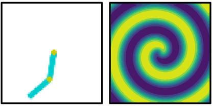
Figure 5: Double pendulum and reaction-diffusion systems.

From high-dimensional and noisy measurements $\mathbf{x}$ of these systems, in our experiments, we aim to (a) denoise of the measurements, (b) learn compact and interpretable representations, (c) predict the dynamics, and (d) quantify uncertainties.

Denoising of Measurements. When dealing with noisy data, an aspect of paramount importance is the ability of the models to remove the noise from the data, that is, denoising. To test the denoising capabilities of our framework, we add Gaussian noise over the measurements:

$$\begin{split}\mathbf{x}_{t}&=\mathbf{x}_{t}+\boldsymbol{\epsilon}_{\mathbf{x}}\\ \boldsymbol{\epsilon}_{\mathbf{x}}&\sim\mathcal{N}(\mathbf{0},\sigma^{2}_{\mathbf{x}}I)\,,\\ \end{split}$$ (20)

where $\sigma^{2}_{\mathbf{x}}\in\{0.0,0.25^{2},0.5^{2}\}$ corresponds to the variance. We aim at recovering the original measurements (see Figure 6 and 10). In addition, to provide a quantitative evaluation, we utilize the peak signal-to-noise ratio (PSNR) and the $L_{1}$ norm to assess the denosing abilities of our method. The PSNR measures the ratio between the maximum possible power of a signal, i.e., $\max(\mathbf{x}^{2}_{t})$, and the power of the corrupting noise, i.e., $||\mathbf{x}_{t}-\hat{\mathbf{x}}_{t}||_{2}^{2}$. The PSNR is defined as:

$$\text{PSNR}=10\cdot\log_{10}\left(\frac{\max(\mathbf{x}_{t}^{2})}{||\mathbf{x}_{t}-\hat{\mathbf{x}}_{t}||_{2}^{2}}\right)\,,$$ (21)

where $\mathbf{x}_{t}$ and $\hat{\mathbf{x}}_{t}$ correspond to the (noisy) measurement and its reconstruction at a generic timestep $t$, respectively. The $L_{1}$ norm measures how close the recovered measurement $\hat{\mathbf{x}}_{t}$ is to the uncorrupted measurement $\mathbf{x}_{t}$. The $L_{1}$ norm is the absolute difference between the original and reconstructed measurements:

$$L_{1}=||\mathbf{x}_{t}-\hat{\mathbf{x}}_{t}||_{1}=|\mathbf{x}_{t}-\hat{\mathbf{x}}_{t}|.$$ (22)

We report these results in Table 1 and 2.

Learning Compact and Interpretable Representations. The second aspect we are interested in is assessing the ability of the framework to learn compact and interpretable latent representations of the system states. To visualize the latent (state) representations, we employ the t-distrubuted stochastic neighbour embedding (t-SNE) method [54] to project the latent states to a 2-dimensional space and inspect their correlation with the true state variables (see Figure 6 and 10).

Predicting the Dynamics. The goal of our method is to learn a ROM that can accurately and efficiently predict the evolution of different dynamical systems. Therefore, after training the model, we evaluate its predictions forward in time by feeding the initial state to the ROM and autoregressively predict the trajectory of the systems. We then compare the predicted trajectories with the trajectories from a test set that were not used for the training of the model (see Figure 8 and 12.

Quantifying Uncertainties. Ultimately, we would like to quantify uncertainties, deriving from the noisy measurements, properly. However, uncertainties over the latent variables are hard to visualize and, consequently analyze [41]. Therefore, we study uncertainties in the measurement space that be more informative then uncertainties over the latent variables. We generate multiple rollouts of the ROM for a fixed initial condition, we decode the latent-space trajectories back to the measurement space using the decoder, we compute standard deviation of the different trajectories, and we plot heatmaps representing the evolution of the uncertainties over time (see Figure 9 and 13).

4.1 Double Pendulum

The first example we consider is an actuated double pendulum. The double pendulum exhibits chaotic and nonlinear behaviour, making the prediction of its dynamics from high-dimensional and noisy measurements extremely challenging. Its dynamics can be described as a function of its joint angles $(\theta_{1},\theta_{2})$, velocities $(\dot{\theta}_{1},\dot{\theta}_{2})$, and accelerations $(\ddot{\theta}_{1},\ddot{\theta}_{2})$. We indicate with $\theta_{1},\theta_{2}$ the angle of the first joint and second joint, $l_{1},l_{2}$ the length of the two links, and $m_{1},m_{2}$ the mass of the two links. The equations of motions of the double pendulum can be written as in state-space form as:

$$\begin{split}\dot{\theta}_{1}&=\omega_{1}\,,\\ \dot{\theta}_{2}&=\omega_{2}\,,\\ \dot{\omega}_{1}&=\frac{-g(2m_{1}+m_{2})\sin\theta_{1}-m_{2}g\sin(\theta_{1}-2\theta_{2})-2\sin(\theta_{1}-\theta_{2})m_{2}(\omega_{2}^{2}l_{2}+\omega_{1}^{2}l_{1}\cos(\theta_{1}-\theta_{2}))}{l_{1}(2m_{1}+m_{2}-m_{2}\cos(2\theta_{1}-2\theta_{2}))}+u_{1}\,,\\ \dot{\omega}_{2}&=\frac{2\sin(\theta_{1}-\theta_{2})(\omega_{1}^{2}l_{1}(m_{1}+m_{2})+g(m_{1}+m_{2})\cos\theta_{1}+\omega_{2}^{2}l_{2}m_{2}\cos(\theta_{1}-\theta_{2}))}{l_{2}(2m_{1}+m_{2}-m_{2}\cos(2\theta_{1}-2\theta_{2}))}\,,\\ \end{split}$$ (23)

where $\omega_{1}$ and $\omega_{2}$ are the angular velocities of the first and second link of the double pendulum, respectively, and $u_{1}$ the control input (torque) to the first joint. The measurements $\mathbf{x}$ are high-dimensional snapshots of dimension $84\times 84\times 3$ of the double pendulum dynamics (see Equation (23)) when a random control $u_{1}$ is applied. An example of measurement is shown in Figure 5 (left).

In Figure 6, we show the reconstructions $\hat{\mathbf{x}}_{t}$ and $\hat{\mathbf{x}}_{t+1}$ for different levels of noise of the measurements $\sigma^{2}_{\mathbf{x}}\in\{0,0.25^{2},0.5^{2}\}$. In this case, we set the latent dimension $|\mathbf{z}|=20$ and the history length $H=20$. As shown by the results, the model can properly denoise the noisy measurements, even in the case of high levels of noise ($\sigma^{2}_{\mathbf{x}}=0.5^{2}$).The ability to remove the noise from the measurements derives from the ability of the model to encode the relevant features into the latent state.

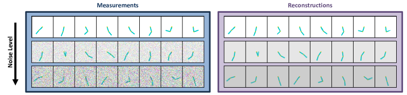
Figure 6: Reconstructions of $\hat{\mathbf{x}}_{t}$ with noise levels $\sigma^{2}_{\mathbf{x}}\in\{0,0.25^{2},0.5^{2}\}$ applied to input measurements. The noise level increases from the top to the bottom images.

To further understand the effect of the recurrent SVDKL architecture on the prediction performance of the ROM, we quantitatively analyse, using the PSNR and L₁ metric , the quality of the reconstructions $\hat{\mathbf{x}}_{t}$ and $\hat{\mathbf{x}}_{t+1}$. The results for different values of $H$, where $H=1$ corresponds to the original architecture proposed in [41], and noise variance $\sigma^{2}_{\mathbf{x}}$ are reported in Table 1. Increasing the history length $H$ improves the encoding and latent model performance and consequently denoising abilities of the model. However, due to the sequential nature of the LSTM, longer input sequences requires more computations and may slow down the training. We found that a value of $H\in[10,20]$ provides a good trade-off between results and computational burden.

Noise Level	Reconstruction $\hat{\mathbf{x}}_{t}$	Reconstruction $\hat{\mathbf{x}}_{t+1}$
$\sigma^{2}_{\mathbf{x}}=0.0$	$H$ $T$ PSNR (db) L1 1 3 29.12 53.74 10 3 33.20 22.25 20 3 31.89 22.71	$H$ $T$ PSNR (db) L1 1 3 21.72 208.00 10 3 31.33 32.18 20 3 30.21 37.50
$\sigma^{2}_{\mathbf{x}}=0.25^{2}$	$H$ $T$ PSNR (db) L1 1 3 26.97 86.15 10 3 29.26 62.39 20 3 29.45 60.14	$H$ $T$ PSNR (db) L1 1 3 22.98 180.30 10 3 28.19 74.69 20 3 28.44 72.55
$\sigma^{2}_{\mathbf{x}}=0.5^{2}$	$H$ $T$ PSNR (db) L1 1 3 23.59 179.97 10 3 24.58 155.60 20 3 24.77 150.84	$H$ $T$ PSNR (db) L1 1 3 20.23 322.15 10 3 24.46 159.01 20 3 24.59 156.12

Table 1: Quantitative results in the case of the double pendulum for different values of $H$. All the models are trained using the loss function in Equation (19) with $T=3$.

In Figure 7, we show the latent variables for different value of noise applied to the measurements. Due to the strong denoising capabilities of our model, the latent representations, visualized via t-SNE, are minimally affected and their correlation with the true variables of the systems, i.e. the angles $\theta_{1}$ and $\theta_{2}$, remains high. Again, we show the results for $|\mathbf{z}|=20$ and $H=20$.

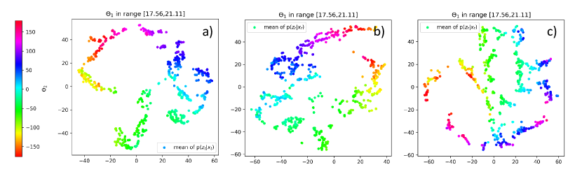
Figure 7: t-SNE visualisation of the mean of the latent state distribution for different levels of noise $\sigma^{2}_{\mathbf{x}}\in\{0,0.25^{2},0.5^{2}\}$ on the measurements, Figure a), b), and c), respectively. The first angle $\theta_{1}$ is fixed within a range, while the colour bar represents the second angle $\theta_{2}$.

To assess the prediction capability of the proposed ROM, we predict the dynamics forward in time from a history of measurements of length $H$. In Figure 8, we show the reconstruction of the predicted trajectories in comparison with the true ones from the test set.

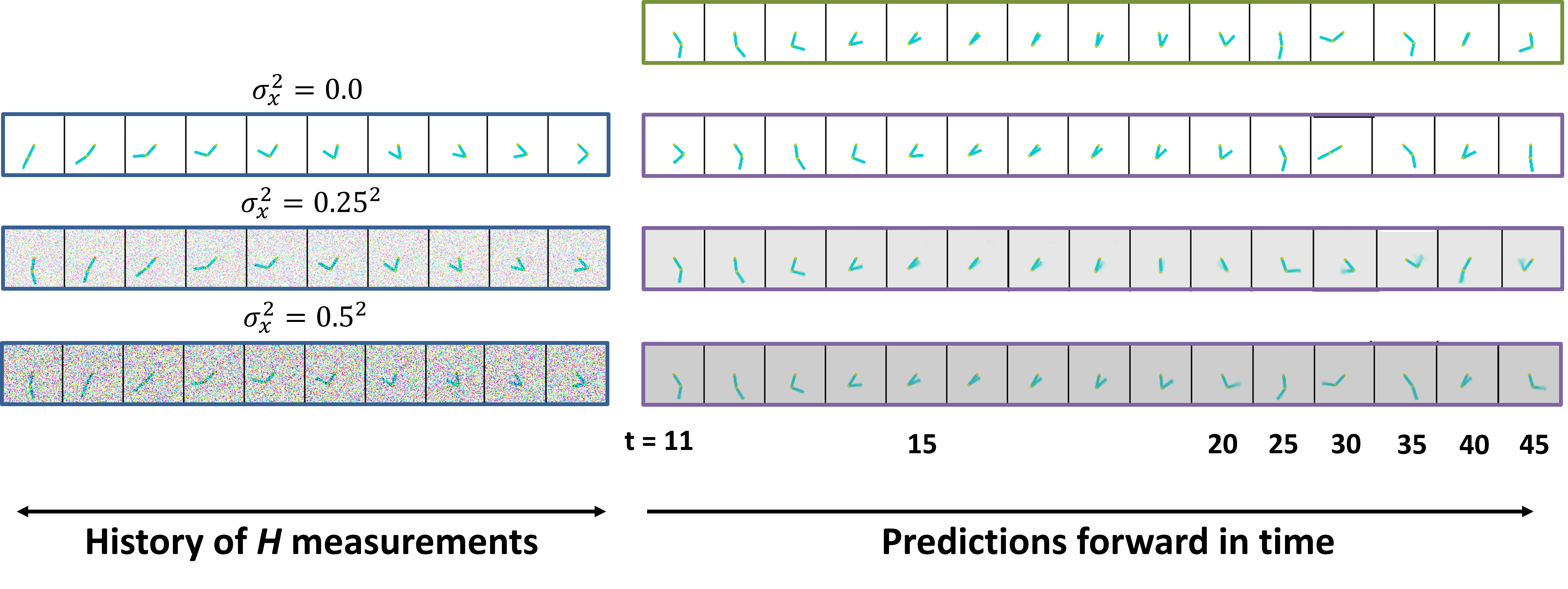
Figure 8: Predictions of the dynamic $\hat{\mathbf{x}}_{t}$ (purple box) for different noise levels $\sigma^{2}_{\mathbf{x}}\in\{0,0.25^{2},0.5^{2}\}$ applied to input measurements (blue box). The true trajectory is highlighted by the green box.

The reconstructions remain close to the true measurements, even with the highest noise level ($\sigma^{2}_{\mathbf{x}}=0.5^{2}$) for the first 20 timesteps. Afterwards, especially in the noisy-measurement cases, we notice a gradual divergence. However, it is worth mentioning that the double pendulum is a chaotic systems and small perturbations of the initial conditions generate drastically different trajectories. Therefore, it is natural to observe this behaviour, especially with additive noise on the measurements acting as a perturbation of the initial conditions.

In Figure 9, we show the uncertainty quantification capabilities of our framework by analyzing the uncertainties over the same trajectory with different noise levels ($\sigma^{2}_{\mathbf{x}}=0.0$ and $\sigma^{2}_{\mathbf{x}}=0.5^{2}$).

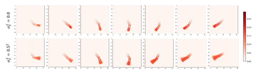
Figure 9: Evolution over time of the standard deviation of the trajectories projected in the image space for $\sigma^{2}_{\mathbf{x}}=0.0$ and $\sigma^{2}_{\mathbf{x}}=0.5^{2}$.

It is possible to notice that the model is sensitive to the noise added to the measurements, as the standard deviation of the predicted trajectory grows with more noise, i.e., the pendulum position is more blurred in the case of $\sigma^{2}_{\mathbf{x}}=0.5^{2}$ than in the case of $\sigma^{2}_{\mathbf{x}}=0.0$.

4.2 Nonlinear Reaction-Diffusion Problem

The second example we consider is a lambda–omega reaction–diffusion system that can be used to describe a wide variety of physical phenomena, spanning from chemistry to biology and geology. The equations describing the dynamics can be written as:

$$\begin{split}\dot{u}&=(1-(u^{2}+v^{2}))u+\beta(u^{2}+v^{2})v+d(u_{xx},u_{yy})\,,\\ \dot{v}&=\beta(u^{2}+v^{2})u+(1-(u^{2}+v^{2}))v+d(v_{xx},v_{yy})\,,\\ \end{split}$$ (24)

where $u=u(x,y,t)$ and $v=v(x,y,t)$ describe the evolution of the spiral wave over time in the spatial domain $(x,y)\in[-10,10]$, and $\beta$ and $d$ are the parameters regulating the reaction and diffusion behaviour of the system, respectively. Our parameter of interest is $\beta$, varying in the range $[0.5,1.5]$. Similarly to [55], we assume periodic boundary conditions and initial condition equal to:

$$u(x,y,0)=v(x,y,0)=\tanh(\sqrt{x^{2}+y^{2}}\cos((x+iy)-\sqrt{x^{2}+y^{2}}).$$ (25)

In this case, the measurements $\mathbf{x}$ are obtained by spatially discretizing the PDE with a $128\times 128$ grid.

In Figure 10, we show the reconstructions $\hat{\mathbf{x}}_{t}$ and $\hat{\mathbf{x}}_{t+1}$ for different levels of noise of the measurements $\sigma^{2}_{\mathbf{x}}\in\{0,0.25^{2},0.5^{2}\}$. Similarly to the double pendulum example, we set the latent dimension $|\mathbf{z}|=20$ and the history length $H=20$. As shown in Figure 10, the model can properly denoise the noisy measurements, even in the case of high levels of noise ($\sigma^{2}_{\mathbf{x}}=0.5^{2}$).

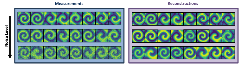
Figure 10: Reconstructions of $\hat{\mathbf{x}}_{t}$ with noise levels $\sigma^{2}_{\mathbf{x}}\in\{0,0.25^{2},0.5^{2}\}$ applied to input measurements. The noise level increases from the top to the bottom images.

Similarly to the case of the double pendulum, we quantitatively analyse, using the PSNR and L₁ metrics, the quality of the reconstructions $\hat{\mathbf{x}}_{t}$ and $\hat{\mathbf{x}}_{t+1}$. The results for different values of $H$, where $H=1$ corresponds to the original architecture proposed in [41], and noise $\sigma^{2}_{\mathbf{x}}$ are reported in Table 2. Even in the reaction-diffusion PDE, increasing the history length $H$ improves the encoding and latent model performance and consequently denoising abilities of the model.

	State reconstruction $\hat{\mathbf{x}}_{t}$	Next state reconstruction $\hat{\mathbf{x}}_{t+1}$
$\sigma_{\mathbf{x}}^{2}=0.0$	$H$ $T$ PSNR (db) L1 1 3 29.32 347.91 10 3 29.29 360.26 20 3 29.34 342.73	$H$ $T$ PSNR (db) L1 1 3 29.30 352.20 10 3 29.05 401.94 20 3 29.31 344.89
$\sigma_{\mathbf{x}}^{2}=0.25^{2}$	$H$ $T$ PSNR (db) L1 1 3 26.55 1029.88 10 3 26.52 1039.02 20 3 26.50 1042.06	$H$ $T$ PSNR (db) L1 1 3 26.56 1024.53 10 3 26.50 1040.52 20 3 26.54 1030.01
$\sigma_{\mathbf{x}}^{2}=0.5^{2}$	$H$ $T$ PSNR (db) L1 1 3 19.82 2947.03 10 3 19.83 2940.93 20 3 19.85 2945.56	$H$ $T$ PSNR (db) L1 1 3 19.88 2923.69 10 3 19.84 2939.25 20 3 19.82 2943.92

Table 2: Quantitative results in the case of the reaction-diffusion PDE for different values of $H$. All the models are trained using the loss function in Equation (19) with $T=3$.

In Figure 11, we show the latent variables for different value of noise applied to the measurements. Similarly to the pendulum example, due to the strong denoising capabilities of our model, the latent representations, visualized via t-SNE, are minimally affected by the noise. This aspect can be noticed by the fact that the latent representations do no qualitatively change for different levels of noise. Again, we show the results for $|\mathbf{z}|=20$ and $H=20$.

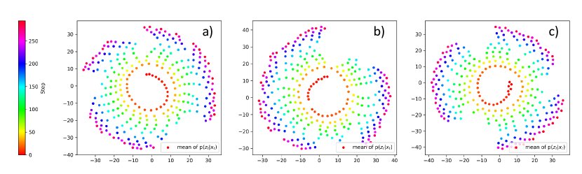
Figure 11: t-SNE visualisation of the mean of the latent state distribution for different levels of noise $\sigma^{2}_{\mathbf{x}}\in\{0,0.25^{2},0.5^{2}\}$ on the measurements, Figure a), b), and c), respectively. The colorbar represents the timestep.

To assess the prediction capability of the proposed ROM, we predict the dynamics forward in time from a history of measurements of length $H$. In Figure 12, we show the reconstruction of the predicted trajectories in comparison with the true ones from the test set.

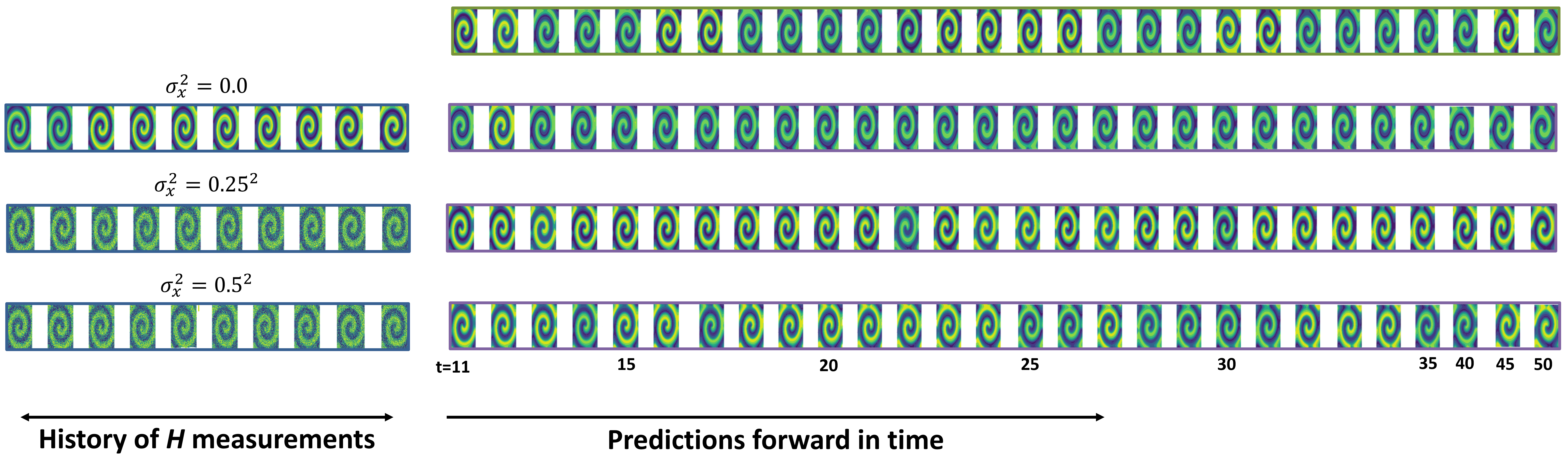
Figure 12: Predictions of the dynamic $\hat{\mathbf{x}}_{t}$ (purple box) for different noise levels $\sigma^{2}_{\mathbf{x}}\in\{0,0.25^{2},0.5^{2}\}$ applied to input measurements (blue box). The true trajectory is highlighted by the green box.

The reconstructions remain close to the true measurements, even with the highest noise level ($\sigma_{\mathbf{x}}^{2}=0.5^{2}$).

In Figure 13, we show the uncertainty quantification capabilities of our framework by analyzing the uncertainties over the same trajectory with different noise levels ($\sigma^{2}_{\mathbf{x}}=0.0$ and $\sigma^{2}_{\mathbf{x}}=0.5^{2}$).

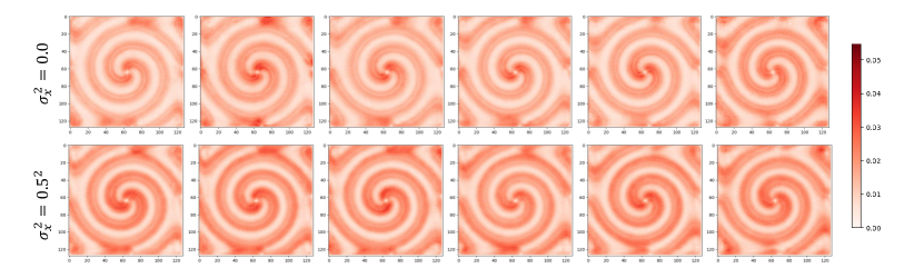
Figure 13: Evolution over time of the standard deviation of the trajectories projected in the image space for $\sigma^{2}_{\mathbf{x}}=0.0$ and $\sigma^{2}_{\mathbf{x}}=0.5^{2}$.

Again, it is possible to notice that the model is sensitive to the noise added to the measurements, as the standard deviation of the predicted trajectory grows with more noise, i.e., the pendulum position is more blurred in the case of $\sigma^{2}_{\mathbf{x}}=0.5^{2}$ than in the case of $\sigma^{2}_{\mathbf{x}}=0.0$.

5 Conclusion

In this paper, we introduced a recurrent SVDKL architecture for learning ROMs for chaotic dynamical systems from high-dimensional and noisy measurements. This novel approach extends the architecture proposed in [41] with a recurrent network and two multi-step loss functions to improve the reliability of the long-term predictions of the latent dynamical SVDKL model. The method was tested on an actuated double pendulum and a parametric reaction-diffusion PDE. Our method, in both test cases, is capable of properly denoising the measurement, learning interpretable latent representations, and consistently predicting the evolution of the systems. Eventually, we propose a way to visualize and analyze the uncertainties quantification capabilities of the framework.

References

- [1] Michael Grieves. Digital twin: manufacturing excellence through virtual factory replication. White paper, 1(2014):1–7, 2014.
- [2] Fei Tao, He Zhang, Ang Liu, and Andrew YC Nee. Digital twin in industry: State-of-the-art. IEEE Transactions on industrial informatics, 15(4):2405–2415, 2018.
- [3] Engineering National Academies of Sciences, Medicine, et al. Foundational research gaps and future directions for digital twins. 2023.
- [4] Karen Willcox and Brittany Segundo. The role of computational science in digital twins. Nature Computational Science, 4(3):147–149, 2024.
- [5] Bruno Sudret and Armen Der Kiureghian. Stochastic finite element methods and reliability: a state-of-the-art report. Department of Civil and Environmental Engineering, University of California …, 2000.
- [6] Tan Bui-Thanh, Karen Willcox, and Omar Ghattas. Parametric reduced-order models for probabilistic analysis of unsteady aerodynamic applications. AIAA journal, 46(10):2520–2529, 2008.
- [7] David Galbally, Krzysztof Fidkowski, Karen Willcox, and Omar Ghattas. Non-linear model reduction for uncertainty quantification in large-scale inverse problems. International journal for numerical methods in engineering, 81(12):1581–1608, 2010.
- [8] Sivaguru S Ravindran. A reduced-order approach for optimal control of fluids using proper orthogonal decomposition. International journal for numerical methods in fluids, 34(5):425–448, 2000.
- [9] Federico Negri, Gianluigi Rozza, Andrea Manzoni, and Alfio Quarteroni. Reduced basis method for parametrized elliptic optimal control problems. SIAM Journal on Scientific Computing, 35(5):A2316–A2340, 2013.
- [10] Fredi Tröltzsch. Optimal control of partial differential equations: theory, methods and applications, volume 112. American Mathematical Society, 2024.
- [11] Andrea Manzoni, Alfio Quarteroni, and Gianluigi Rozza. Shape optimization for viscous flows by reduced basis methods and free-form deformation. International Journal for Numerical Methods in Fluids, 70(5):646–670, 2012.
- [12] Tiangang Cui, Youssef M Marzouk, and Karen E Willcox. Data-driven model reduction for the bayesian solution of inverse problems. International Journal for Numerical Methods in Engineering, 102(5):966–990, 2015.
- [13] Michalis Frangos, Youssef Marzouk, Karen Willcox, and Bart van Bloemen Waanders. Surrogate and reduced-order modeling: a comparison of approaches for large-scale statistical inverse problems. Large-Scale Inverse Problems and Quantification of Uncertainty, pages 123–149, 2010.
- [14] Yanhua Cao, Jiang Zhu, I Michael Navon, and Zhendong Luo. A reduced-order approach to four-dimensional variational data assimilation using proper orthogonal decomposition. International Journal for Numerical Methods in Fluids, 53(10):1571–1583, 2007.
- [15] Yvon Maday, Anthony T Patera, James D Penn, and Masayuki Yano. A parameterized-background data-weak approach to variational data assimilation: formulation, analysis, and application to acoustics. International Journal for Numerical Methods in Engineering, 102(5):933–965, 2015.
- [16] Alfio Quarteroni, Andrea Manzoni, and Federico Negri. Reduced basis methods for partial differential equations: an introduction, volume 92. Springer, 2015.
- [17] Athanasios C Antoulas, Danny C Sorensen, and Serkan Gugercin. A survey of model reduction methods for large-scale systems. Technical report, 2000.
- [18] Peter Benner, Serkan Gugercin, and Karen Willcox. A survey of projection-based model reduction methods for parametric dynamical systems. SIAM review, 57(4):483–531, 2015.
- [19] Kevin Carlberg, Ray Tuminaro, and Paul Boggs. Preserving lagrangian structure in nonlinear model reduction with application to structural dynamics. SIAM Journal on Scientific Computing, 37(2):B153–B184, 2015.
- [20] Jan S Hesthaven, Gianluigi Rozza, Benjamin Stamm, et al. Certified reduced basis methods for parametrized partial differential equations, volume 590. Springer, 2016.
- [21] Bernd R Noack, Michael Schlegel, Marek Morzynski, and Gilead Tadmor. Galerkin method for nonlinear dynamics. In Reduced-order modelling for flow control, pages 111–149. Springer, 2011.
- [22] Bernd R Noack, Marek Morzynski, and Gilead Tadmor. Reduced-order modelling for flow control, volume 528. Springer Science & Business Media, 2011.
- [23] Peter J Schmid. Dynamic mode decomposition of numerical and experimental data. Journal of fluid mechanics, 656:5–28, 2010.
- [24] Steven L Brunton and J Nathan Kutz. Data-driven science and engineering: Machine learning, dynamical systems, and control. Cambridge University Press, 2019.
- [25] Omar Ghattas and Karen Willcox. Learning physics-based models from data: perspectives from inverse problems and model reduction. Acta Numerica, 30:445–554, 2021.
- [26] Mengwu Guo, Shane A McQuarrie, and Karen E Willcox. Bayesian operator inference for data-driven reduced-order modeling. Computer Methods in Applied Mechanics and Engineering, 402:115336, 2022.
- [27] Benjamin Peherstorfer and Karen Willcox. Data-driven operator inference for nonintrusive projection-based model reduction. Computer Methods in Applied Mechanics and Engineering, 306:196–215, 2016.
- [28] Elizabeth Qian, Boris Kramer, Benjamin Peherstorfer, and Karen Willcox. Lift & learn: Physics-informed machine learning for large-scale nonlinear dynamical systems. Physica D: Nonlinear Phenomena, 406:132401, 2020.
- [29] Joseph Bakarji, Kathleen Champion, J Nathan Kutz, and Steven L Brunton. Discovering governing equations from partial measurements with deep delay autoencoders. arXiv preprint arXiv:2201.05136, 2022.
- [30] Steven L Brunton, Joshua L Proctor, and J Nathan Kutz. Discovering governing equations from data by sparse identification of nonlinear dynamical systems. Proceedings of the national academy of sciences, 113(15):3932–3937, 2016.
- [31] Kathleen Champion, Bethany Lusch, J Nathan Kutz, and Steven L Brunton. Data-driven discovery of coordinates and governing equations. Proceedings of the National Academy of Sciences, 116(45):22445–22451, 2019.
- [32] Paolo Conti, Giorgio Gobat, Stefania Fresca, Andrea Manzoni, and Attilio Frangi. Reduced order modeling of parametrized systems through autoencoders and sindy approach: continuation of periodic solutions. Computer Methods in Applied Mechanics and Engineering, 411:116072, 2023.
- [33] L Gao and J Nathan Kutz. Bayesian autoencoders for data-driven discovery of coordinates, governing equations and fundamental constants. arXiv preprint arXiv:2211.10575, 2022.
- [34] Hayden Schaeffer. Learning partial differential equations via data discovery and sparse optimization. Proceedings of the Royal Society A: Mathematical, Physical and Engineering Sciences, 473(2197):20160446, 2017.
- [35] Stefania Fresca, Luca Dede’, and Andrea Manzoni. A comprehensive deep learning-based approach to reduced order modeling of nonlinear time-dependent parametrized pdes. Journal of Scientific Computing, 87:1–36, 2021.
- [36] Stefania Fresca and Andrea Manzoni. Pod-dl-rom: Enhancing deep learning-based reduced order models for nonlinear parametrized pdes by proper orthogonal decomposition. Computer Methods in Applied Mechanics and Engineering, 388:114181, 2022.
- [37] Kookjin Lee and Kevin T Carlberg. Model reduction of dynamical systems on nonlinear manifolds using deep convolutional autoencoders. Journal of Computational Physics, 404:108973, 2020.
- [38] Samuel E Otto and Clarence W Rowley. Linearly recurrent autoencoder networks for learning dynamics. SIAM Journal on Applied Dynamical Systems, 18(1):558–593, 2019.
- [39] Qinyu Zhuang, Juan Manuel Lorenzi, Hans-Joachim Bungartz, and Dirk Hartmann. Model order reduction based on runge–kutta neural networks. Data-Centric Engineering, 2:e13, 2021.
- [40] Mengwu Guo and Jan S Hesthaven. Data-driven reduced order modeling for time-dependent problems. Computer methods in applied mechanics and engineering, 345:75–99, 2019.
- [41] Nicolò Botteghi, Mengwu Guo, and Christoph Brune. Deep kernel learning of dynamical models from high-dimensional noisy data. Scientific reports, 12(1):21530, 2022.
- [42] Yann LeCun, Yoshua Bengio, and Geoffrey Hinton. Deep learning. nature, 521(7553):436–444, 2015.
- [43] Ian Goodfellow, Yoshua Bengio, and Aaron Courville. Deep learning. MIT press, 2016.
- [44] Christopher KI Williams and Carl Edward Rasmussen. Gaussian processes for machine learning, volume 2. MIT press Cambridge, MA, 2006.
- [45] Andrew Gordon Wilson, Zhiting Hu, Ruslan Salakhutdinov, and Eric P Xing. Deep kernel learning. In Artificial intelligence and statistics, pages 370–378. PMLR, 2016.
- [46] Andrew G Wilson, Zhiting Hu, Russ R Salakhutdinov, and Eric P Xing. Stochastic variational deep kernel learning. Advances in neural information processing systems, 29, 2016.
- [47] David M Blei, Alp Kucukelbir, and Jon D McAuliffe. Variational inference: A review for statisticians. Journal of the American statistical Association, 112(518):859–877, 2017.
- [48] Ethan Goan and Clinton Fookes. Bayesian neural networks: An introduction and survey. Case Studies in Applied Bayesian Data Science: CIRM Jean-Morlet Chair, Fall 2018, pages 45–87, 2020.
- [49] Bruce E Rosen. Ensemble learning using decorrelated neural networks. Connection science, 8(3-4):373–384, 1996.
- [50] Diederik P Kingma and Max Welling. Auto-encoding variational bayes. arXiv preprint arXiv:1312.6114, 2013.
- [51] Danijar Hafner, Timothy Lillicrap, Ian Fischer, Ruben Villegas, David Ha, Honglak Lee, and James Davidson. Learning latent dynamics for planning from pixels, 2019.
- [52] Danijar Hafner, Timothy Lillicrap, Jimmy Ba, and Mohammad Norouzi. Dream to control: Learning behaviors by latent imagination. arXiv preprint arXiv:1912.01603, 2019.
- [53] Alex Graves and Alex Graves. Long short-term memory. Supervised sequence labelling with recurrent neural networks, pages 37–45, 2012.
- [54] Laurens Van der Maaten and Geoffrey Hinton. Visualizing data using t-sne. Journal of machine learning research, 9(11), 2008.
- [55] Paolo Conti, Mengwu Guo, Andrea Manzoni, Attilio Frangi, Steven L Brunton, and J Nathan Kutz. Multi-fidelity reduced-order surrogate modeling. arXiv preprint arXiv:2309.00325, 2023.