Phase Transitions in the Anisotropic Dicke-Stark Model with -square terms
Abstract
The superradiant phase transition (SRPT) is forbidden in the standard isotropic Dicke model due to the so-called no-go theorem induced by -square term. In the framework of the Dicke model, we demonstrate that SRPTs can occur at both zero and finite temperatures if we intrinsically tune the rotating wave and count-rotating atom-cavity coupling independently, and/or introduce the nonlinear Stark coupling terms, thus overcoming the no-go theorem. The phase transitions in this so-called anisotropic Dicke-Stark model share the same universality class with the original Dicke model. The critical coupling strength of this model decreases with the isotropic constant gradually, but can be driven to zero quickly with the strong nonlinear Stark coupling. We believe that we have proposed a feasible scheme to observe the SRPT in the future solid-state experiments.
pacs:
42.50.Pq, 68.35.Rh, 05.30.Rt, 64.75.-gI Introduction
The Dicke model describes a collection of two-level atoms interacting with a single radiation mode via an atom-field coupling DM . The thermal phase transition (TPT) from the normal phase to the superradiant phase in equilibrium was predicted more than 50 years ago DM_PT ; DM_PT2 . In 2003, the quantum phase transition (QPT) was also theoretically studied emary2003prl , which exhibit the mean-field nature. However both TPT and QPT in equilibrium have never been convincingly observed in the experiments which are solely described by the original Dicke model. Although it was reported that the superradiant phase transition (SPT) was observed in Bose-Einstein condensates (BEC) in optical cavities Baumann and simulation via cavity-assisted Raman transitions Zhiqiang , it was shown later that these two realizations of the superradiant transition in the Dicke model involve driven-dissipative systems, thus they are not the equilibrium but the non-equilibrium phase transitions Torre2018intro . By analyzing the average number of photons, it was found in Ref. Dalla that the critical scaling exponent for photons in the driven-dissipative Dicke model is different from that in equilibrium Dicke model Liu . It follows that the emergence of the photons in experiments is not a sufficient evidence of the equilibrium phase transitions.
One of the major challenge to realize the equilibrium superradiant phase transition (SRPT) is that it only occurs at the very strong atom-cavity coupling, which seems almost not accessible in the recent stongly light-matter interaction systems based on some advanced solid-state platforms, except in the quantum simulations. To takle this problem, two of the present authors and collaborators have introduced the interaction between atoms taoliu2012pla to reduce the critical strength.
The most serious difficulty is however rooted in a fundamental issue that the dipole coupling between the atoms and the cavity may be incompletely considered in the standard Dicke model. So even from a theoretical perspective, it is still in debate to realize the SRPT experimentally A2original ; keeling2007jpb ; vukics2014prl ; ciuti2010nc ; viehmann2011prl ; ciuti2012prl ; viehmann_arxiv ; rabl2016pra ; bamba2016prl ; bamba2017pra ; andolina2019prb ; nori2019np ; nazir2020prl ; nazir2022rmp . In the cavity quantum electrodynamical (QED), Rzażeskimo et al. argued that the so-called -square term originated from minimal coupling Hamiltonian would forbid the SRPT of the Dicke model at any finite coupling strength if the Thomas-Reich-Kahn (TRK) sum rule for atom is taken into account properly A2original . According to the effective model of the circuit QED, Nataf and Ciuti proposed that the TRK sum rule of the cavity QED could be violated and the SRPT may occur in principle ciuti2010nc . Viehmann et al. questioned that even within a complete microscopic treatment, the no-go theorem of the cavity QED still applies to the circuit QED viehmann2011prl . These arguments focus on whether the TRK sum rule changes in different systems viehmann2011prl ; ciuti2012prl , which arouse a huge controversy whether the -square term can be engineered in the superconductive qubit circuit platform viehmann_arxiv ; rabl2016pra ; bamba2016prl ; andolina2019prb . A specific circuit configuration was also designed to generate the SRPT bamba2016prl ; bamba2017pra . On the other hand, because the validity of the two-level approximation is the key step of constructing the Dicke model in various solid-state devices, the applicability of Coulomb and electric dipole gauges, and different experimental schemes leading to different -square terms are also widely discussed in the literature ( see Stefano ; Stokes ; Andolina , and the references therein). Consensus has not been reached yet, and the no-go theorem is still the most controversial subject.
We would not join the debate of the existence of the -square terms subject to the TRK sum rule. In the present work, keeping such a -square term, we propose an effective scheme to realize the SRPT in the original Dicke model at weak atom-cavity coupling by manipulating the inner factors. In the framework of the standard Dicke model which only consists of two ingredients: two-level atoms without mutual interactions and single-mode cavity, what we can do is to modify the atom-cavity interactions. In doing so, we first relax the isotropic atom-cavity interaction to the anisotropic one, i.e. the coupling strengths of the rotating and counterrotating wave terms are different.Such an anisotropic Dicke model can be implemented in the cavity and circuit QED Ciute2 ; mxliu2017prl . On the other hand, Grimsmo and Parkins proposed that a nonlinear atom-cavity coupling, nowadays called the Stark coupling, can be realized in an experimental set-up with two hyperfine ground states of a multilevel atom coupled to a quantized cavity field and two auxiliary laser fields. Generalizations of the Stark coupling into the Dicke model gives the so-called Dicke-Stark model (DSM). It is found in KeelingPRL2010 ; KelingPRA2012 that the critical coupling strength of the none-equilibrium QPT of the DSM is very sensitive to the nonlinear Stark interaction between atoms and cavity. So we then incorporate the Stark coupling terms in the anisotropic Dicke model and try to reduce the critical strength of the equilibrium SRPT, so that the SRPT may be feasible in the future advanced experiments.
The paper is organized as follows: In Sec. II, we introduce the Hamiltonian for anisotropic Dicke-Stark model with -square terms . In Sec. III, within the Holstein-Primakoff transformation, we will derive the mean-field critical coupling strength. We will derive a free energy of the general model and discuss the thermal phase transitions in Sec. III. Finally, conclusions are drawn in Sec. V. Appendix A and B will presents some analytical derivation and numerical confirmations.
The paper is organized as follows: In Sec. II, we introduce the Hamiltonian for anisotropic Dicke-Stark model with -square terms . In Sec. III, within the Holstein-Primakoff transformation, we will derive the mean-field critical coupling strength. We will derive a free energy of the general model and discuss the thermal phase transitions in Sec. III. Finally, conclusions are drawn in Sec. V. Appendix A and B will presents some analytical derivation and numerical confirmations.
II The anisotropic Dicke-Stark model with -square term
We consider an anisotropic Dicke-Stark model, which describes a collection of two-level systems coupled to a bosonic field by adding a stark shift term to the anisotropic Dicke model. The Hamiltonian is given by
| (1) | ||||
| (2) |
where is the anisotropic Dicke Hamiltonian, and -term is the stark shift term for the nonlinear atom-cavity interactions. creates (annihilate) one photon in the common single-mode cavity with frequency , is the transition frequency of each two-level atom. The angular momentum operator represents the collective pesudospin associated to the collection of two-level atoms, . The counter-roatating-wave (CRW) interacting terms and do not conserve the number of excitations, while the rotating-wave (RW) terms and lead to conserved excitations. The anisotropic coupling is tuned by , which is the ratio of the CRW to the RWA coupling strength , which plays a crucial role in the SRPT.
Note that the term of the Hamiltonian represents an -square term imposed by the TRK sum rule for the atoms, which originates from term for an atom coupled to an electromgnetic field with a vector potential . For convenience we set with a dimensionless parameter , for which it is required to satisfy the TRK sum rule A2original . The -square term, often overlooked in other works, will become crucial for the SRPT in the DSM with the additional stark shift term.
III Quantum phase transitions
In order to explore the phase diagram, we perform the Holstein-Primakoff transformation. The angular momentum operators are expressed in terms of bosoic operators and , giving , , an . Then we shift the bosonic operators with respect to their mean value as and . The nonzero value of and are the order parameters of the SRPT, which signal a macroscopic excitation of photons and a spontaneous pseudospn polarization of the two-level atoms. The ground-state energy are obtained by keeping the terms proportional to
| (3) |
Minimizing the ground state energy with respect to and leads to
| (4) |
and
| (5) |
where with . The nontrivial solutions of and are obtained in the superradiant phase, while they are zero in the normal phase. We see that the mean value is real only when . It yields the critical coupling strength of the SRPT
| (6) |
Note that for the isotropic Dicke model , under the TRK sum rule (), no phase transition can occur at a finite coupling strength, which is consistent with the no-go theorem. Very interestingly, for the anisotropic Dicke model, we do find the quantum phase transitions at a finite critical coupling strength under the condition , even constrained by the TRK sum rule. Moreover, the critical coupling strength decreases with , which requires . It indicates that the presence of the nonlinear Stark type atom-cavity interaction can reduce the critical point, demonstrating the feasible superradiant QPT in experiments at the weak atom-cavity coupling.
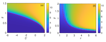
Fig. 1 shows phase diagrams in the and planes of the DSM, respectively. We calculate the mean photon number by numerically exact diagonalizations with atoms. is almost zero below the critical line, and then smoothly increases in the superradiant phase regime. The analytical coupling strength dependent on in Eq. (6) (red dashed line) fits well with the critical phase boundary in Fig. 1 (a). decreases quickly when approaches to . Although the nonlinear Stark coupling is not necessary for the occurrence of the SRPT, it can effectively reduce the critical coupling point in the practical experiments. Moreover, the critical coupling strength increases sharply as the anisptropic ratio tends to in Fig. 1 (b). As an evidence the SRPT is absence for the isotrpic Dicke model due to the restriction of the TRK rule. However, it is possible to observe the emergence of the SRPT by enhancing the anisptropy. The critical line agrees well with the analytical . Consequence the SRPT is accessible with the additional Stark coupling for the anisotropic Dicke model.
It is worth noting that, for , there still exists the superradiant QPT, in sharp contrast to the single-atom Rabi-Stark model where the system is in the continuum in this regime Rabi_stark . It may underline the many-body effect in the Dicke-Stark model. For , the numerical diagonalizations cannot be converged, suggesting that the system is in the continuum, similar to the single-atom Rabi-Stark model.
To explore the critical exponents of the SRPT, we study the finite-size scaling law for a numerical analysis of the scaling behavior. The general finite-size scaling ansatz for an observable around the critical value is given as
| (7) |
where is a scaling function, is the correlation length exponent, and is a scaling exponent dependent on . At the critical value the finite-size scaling becomes with .
| exponent | ||||
|---|---|---|---|---|
| 1/2 | 1 | -1/4 | ||
| -1/3 | -2/3 | 1/6 |
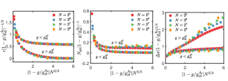
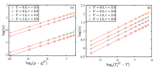
We calculate the scaling exponents of the lowest excitation energy , mean photon number and the variance of the position quadrature of the field , which are obtained by using the numerically exact calculation. Near the critical point, the excitation energy vanishes as , while and diverge as and , respectively. Table 1 show different scaling exponents and of the observables , and . However, the critical exponent is universal and independent on observables.
As expected, the scaling function in Eq.(7) is universal with the critical exponent . The finite-size scaling function of the exictation energy can be given as . Fig.2(a) shows that all the curves of different size collapse into a single curve in the critical regime. An excellent collapse of the scaling function of and are also observed in Fig.2(b) and (c), respectively. The numerical results confirm the validity of the universal exponents of the anisotropic Dicke model, which belongs to the same universality class of the conventional Dicke model.
IV Finite-temperature phase transitions
We investigate the superradiant phase transition at a finite temperature, which is crucial to understand the experiment findings and temperature-dependent physics.
For a finite temperature , the partition function is for the Hamiltonian in Eq.(2) with , where is written in terms of the Hamiltonian of each atom coupled to the cavity , where are Pauli matrices for each atom. Using the mean-field approximation , the Hamiltonian can be given as
| (8) |
The reduced free energy is defined as . With the mean field partition function , the free energy is given by
| (9) |
where is eigenvalue of . The critical value is obtained by the condition
| (10) |
In particular, is valid only if and . The critical value depends on the temperature , and reduces to the critical value at zero temperature in Eq. (6).
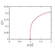
For finite-temperature SRPT, the critical temperature for SRPT is obtained as
| (11) |
Fig. 3 shows the phase diagram at finite temperature. The line of second order phase transition terminates at the quantum critical point at .
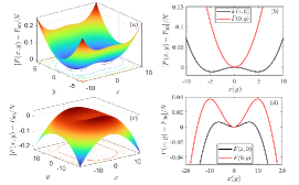
The free energy is crucial to capture the second-order phase transition according to the Landau theory. We generally set a complex in numerical calculation. For the anisotropic case enough large in Fig. 4 (a) and (b) satisfying and , the free energy has two local minimums at nonzero real value of for , while it changes to a single local minimum at below the critical point. It also supports the above derivation that the free energy is expressed as a function of real . It indicates the occurrence of the second-order phase transition. However, for the isotropic case in Fig. 4 (c) and (d), there emerge two local maximum at two complex value of for . It signals an unstate state above the critical point, indicating no superradiant phase transition. Because substituting in Eq. (10) leads negative numerator and denominator of , i.e., and . The numerical results confirm the constraints of the phase transition. It demonstrates that the finite-temperature SRPT is possible to occur in the anisotropic Dicke model with .

The finite-temperature phase transition can be characterized by the parameter , similar to the quantum phase transition. One analytically obtains the value of by minimization the free energy Eq. (9) with respect to , which yields the equation
Fig. 5 shows the order parameter depending on both of the temperature and the coupling strength for different anisotropic coupling ratio and the stark-shift parameter . In Fig. 5 (a), as decreases below , the system enters from the norm phase with to the superradiant phase, and the order parameter grows from zero. For the quantum phase transition with , becomes nonzero as increase above the critical value in Fig. 5 (b). It indicates that there occur both of quantum and classical superradiant phase transition in the anisotropic Dicke-Stark model with -square term.
To study the scaling exponent of the anisotropic Dicke-Stark model at finite temperature, we expect the parameter to vanish with a power-law behavior of the form around the critical point. In particular for the Stark coupling , one easily obtains at zero temperature, resulting in the scaling behavior . In the presence of the nonlinear Stark coupling, we numerically calculate the scaling exponent of due to the absence of the analytical expression of . At , scales as in Fig. (6)(a), where the fitting scaling exponent is . Compared to the finite-temperature case in Fig. (6) (b), one observes with . Thus, both of the quantum and classical phase transition have the same scaling exponent, which is the same as that in the Dicke model at zero temperature (Torre2018intro, ).
V Conclusion
We have investigated the SRPTs at zero temperature and finite temperature for the anisotropic DSM with an additional nonlinear stark coupling and square term. We find that the anisotropic coupling is possible to overcome the constraints of the TRK sum rule, exhibiting the superradiant phase transition. Moreover, the nonlinear Stark coupling reduce the critical value, providing a experimentally feasible scheme. At finite-temperature, the free energy for the anisotropic ratio is split into two local minimum above the critical temperature , indicating the occurrence of the SRPT. In contrast, the free energy of the isotropic model always has a single local minimum at the center, thus exclude the possibility of phase transitions. The scaling exponent of the finite-temperature phase transition is the same as that in the Dicke model at zero temperature. Our study opens a window for the achievement of the superradiant phase transition in the light-matter coupling systems.
Acknowledgements.
This work is supported in part by the National Natural Science Foundation of China (Grants No. 11834005, No. 12075040, No. 12347101 and No. 2022M720387, No. 12305009). National Key R&D Program of China 2022YFA1402701.References
- (1) R. H. Dicke, Phys. Rev. 93, 99 (1954).
- (2) K. Hepp and E. H. Lieb, Ann. Phys. 76, 360 (1973).
- (3) Y. K. Wang, F. T. Hioe, Phys. Rev. A 7, 831 (1973).
- (4) C. Emary and T. Brandes, Phys. Rev. Lett. 90 , 044101 (2003); Phys. Rev. E 67,066203 (2003).
- (5) K. Baumann, C. Guerlin, F. Brennecke & T. Esslinger, Dicke quantum phase transition with a superfluid gas in an optical cavity. Nature (London) 464, 1301 (2010).
- (6) Z. Zhiqiang, C. H. Lee, R. Kumar, K. J. Arnold, S. J. Masson, A. L. Grimsmo, A. S. Parkins, and M. D. Barrett, Dicke-model simulation via cavity-assisted Raman transitions. Phys. Rev. A 97, 043858 (2018).
- (7) E. G. Dalla Torre, S. Diehl, M. D. Lukin, S. Sachdev, and P. Strack, Keldysh approach for nonequilibrium phase transitions in quantum optics: Beyond the Dicke model in optical cavities. Phys. Rev. A 87, 023831 (2013).
- (8) J. Vidal and S. Dusuel, Europhys. Lett. 74, 817 (2006); T. Liu, Y.-Y. Zhang, Q.-H. Chen, and K.-L. Wang, Phys. Rev. A 80, 023810 (2009).
- (9) P. Kirton, M. M. Roses, J. Keeling, E. G. Dalla Torre, Advanced Quantum Technologies, 2018, 2, [ Online; accessed 2024-02-24].
- (10) Q. H. Chen, T. Liu, Y. Y. Zhang, and K. L. Wang, Phys. Rev. A, 82, 053841 (2010).
- (11) K. Rzażewski, K. Wodkiewicz, W. Żakowicz, Phys. Rev. Lett. 35, 432 (1975).
- (12) J. Keeling, J. Phys. Condens. Matter 19, 295213 (2007).
- (13) A. Vukics, T. Grießer, P. Domokos, Phys. Rev. Lett. 112, 073601 (2014).
- (14) P. Nataf and C. Ciuti, Nat. Comm. 1, 72 (2010).
- (15) O. Viehmann, J. von Delft, F. Marquardt, Phys. Rev. Lett. 107, 113602 (2011).
- (16) C. Ciuti and P. Nataf, Phys. Rev. Lett. 109, 179301 (2012).
- (17) O. Viehmann, J. von Delft, F. Marquardt, arXiv, 1202, 2916.
- (18) T. Jaako, Z. L. Xiang, J. J. Garcia-Ripoll, and P. Rabl, Phys. Rev. A 94, 033850 (2016).
- (19) G. M. Andolina, F. M. D. Pellegrino, V. Giovannetti, A. H. MacDonald, and M. Polini, Phys. Rev. B 100, 121109(R) (2019).
- (20) M. Bamba, K. Inomata, and Y. Nakamura, Phys. Rev. Lett. 117, 173601 (2016).
- (21) O. Di Stefano, A. Settineri, V. Macrì, L. Garziano, R. Stassi, S. Savasta, F. Nori, Nat. Phys. 15, 803 (2019).
- (22) A. Stokes and A. Nazir, Phys. Rev. Lett. 125 , 143603 (2020).
- (23) A. Stokes and A. Nazir, Rev. Mod. Phys. 94, 045003 (2022).
- (24) M. Bamba and N. Imoto, Phys. Rev. A 96, 053857 (2017).
- (25) O. Di Stefano, A. Settineri, V. Macrì, L. Garziano, R. Stassi, S. Savasta, F. Nori, Nat. Phys. 15, 803(2019).
- (26) A. Stokes and A. Nazir, Phys. Rev. Lett. 125, 143603 (2020).
- (27) G. M. Andolina, F. M. D. Pellegrino, A. Mercurio, O. Di Stefano, M. Polini, and S. Savasta, arXiv:2104.09468v4.
- (28) A. Baksic and C. Ciuti, Phys. Rev. Lett. 112, 173601 (2014).
- (29) M. X. Liu, S. Chesi, Z. J. Ying, X. Chen, H. G. Luo, and H. Q. Lin, Phys. Rev. Lett. 119, 220601 (2017).
- (30) J. Keeling, M. J. Bhaseen, B. D. Simons, Phys. Rev. Lett., 2010, 105, 043001.
- (31) M. J. Bhaseen, J. Mayoh, B. D. Simons, J. Keeling, Phys. Rev. A, 2012, 85, 013817.
- (32) A. L. Grimsmo and S. Parkins, Phys. Rev. A 87 033814 (2013); A. J. Maciejewski, M. Przybylska, and T. Stachowiak, Phys. Lett. A 379 1503(2015); H. P. Eckle and H. Johannesson, J. Phys. A: Math. Theor. 50, 294004 (2017); Y. F. Xie, L. W. Duan, Q. H. Chen, J. Phys. A: Math. Theor. 52, 245304 (2019); X.-Y. Chen, Y.-F. Xie, Q.-H. Chen,Phys. Rev. A , 2020, 102, 063721; Daniel Braak, Lei Cong, Hans-Peter Eckle, Henrik Johannesson, Elinor K. Twyeffort: arXiv:2403.16758.