Learning Task-relevant Sequence Representations via Intrinsic Dynamics Characteristics in Reinforcement Learning

Abstract

Learning task-relevant state representations is crucial to solving the problem of scene generalization in visual deep reinforcement learning. Prior work typically establishes a self-supervised auxiliary learner, introducing elements (e.g., rewards and actions) to extract task-relevant state information from observations through behavioral similarity metrics. However, the methods often ignore the inherent relationships (e.g., dynamics relationships) between the elements that are essential for learning accurate representations, and they are also limited to one-step metrics, which impedes the discrimination of short-term similar task/behavior information in long-term dynamics transitions. To solve the issues, we propose an intrinsic Dynamic characteristics-driven Sequence Representation learning method (DSR) over a common DRL frame. Concretely, inspired by the fact of state transition in the underlying system, DSR constrains the optimization of the encoder via modeling the dynamics equations related to the state transition, which prompts the latent encoding information to satisfy the state transition process and thereby distinguishes state space and noise space. Further, to refine the ability of encoding similar tasks based on dynamics constraints, DSR also sequentially models inherent dynamics equation relationships from the perspective of sequence elements’ frequency domain and multi-step prediction. Finally, experimental results show that DSR has achieved a significant performance boost in the Distracting DMControl Benchmark, with an average of 78.9% over the backbone baseline. Further results indicate that it also achieves the best performance in real-world autonomous driving tasks in the CARLA simulator. Moreover, the qualitative analysis results of t-SNE visualization validate that our method possesses superior representation ability on visual tasks.

I Introduction

Deep reinforcement learning (DRL) has achieved great success in high-dimensional scenarios such as video games [1], robot operations [2], and autonomous driving [3] due to its ability to feature representation for high-dimensional pixels by the combination of neural networks. However, a serious challenge faced by current DRL is that the policies trained in specific scenes struggle to generalize effectively to unseen scenes [4]. Moreover, it is exacerbated when policies are exposed to diverse scenarios. To tackle this challenge, previous work usually studies effective state representation learners to extract a representation space that can summarize task-relevant details within the environment, thus enabling the learning of generalizable policies [5].

Early efforts to enhance DRL’s representation abilities have widely employed data augmentation techniques in the representation learning process [6]. Numerous studies utilize data augmentation to generate diverse images to capture latent invariant information in anchor observations, thereby discarding task-irrelevant components in the scene. To be specific, most of these works are guided by the principle of noise contrast estimation (NCE), which achieves understanding between task and noise by optimizing the Q-learning gradients with data augmentation (e.g., CG2A [7] and DrQ [8]), the temporal difference error (e.g., SVEA [9] and SGQN [10]), and the mutual information between pairs of positive and negative samples, (e.g., TACO [11] and CURL [12]). Additionally, some studies have proposed cyclic augmentation (CycAug) [13] and convolutional augmentation (Conv) [9] to enrich the spatial diversity in some scenarios. Essentially, the primary aim of data augmentation is to incorporate various optimization or approximation methods to distinguish between semantically variant and invariant features in original and augmented observations [7, 14]. However, these methods heavily rely on manually designed augmentation noises with weak universality. Moreover, it is impractical to design a sufficient number of augmentation patterns to content with the generalization demands of real-world scenarios [15].

Compared to data augmentation, Behavioral Similarity Metric (BSM) representation learning [16] is more broadly applicable and requires no augmentation noise. its core idea lies in utilizing inherent elements (e.g., rewards) on Markov decision process (MDP) of the DRL system to quantify task-equivalent information in noisy observations. For instance, the representative deep bisimulation metric (DBC) [14], optimizes a compact representation of the observation space by the distance of rewards and transition distributions. However, such strict distances are difficult to optimize in practice, often requiring conservative calculations [17] or relaxation [18] of these element distances. Further, other works also investigate bisimulation-based clustering representation [19] and action-based similarity metric [20]. Despite these efforts, the above metric-based methods ignore the inherent relationships or constraints (e.g., dynamics relationships) between different elements [21]. Specifically, they typically optimize the distances of rewards, actions, or transition states independently, making it difficult for the representation information to meet underlying dynamics relationships and potentially losing useful information [17]. Also, they are limited to one-step predictions, which cannot effectively distinguish observations with similar task information [22]. For example, for two observations with the same reward or policy distributions, one-step methods may incorrectly infer that they are bi-simulation, which leads to premature collapse of the encoding space.

To address these issues, we propose a sequence state representation method driven by the intrinsic dynamics characteristics [23] of DRL to separate the state space and noise space in observations. Overall, it uses the dynamics equations related to the fact of the state transition to constrain the optimization of the state encoder, which ensures that the encoded information progressively approximates the real state that obeys the state transition process. We illustrate our motivation with Figure 1. Specifically, in the DRL interactions, as actions are executed, the task-relevant state parts in the underlying DRL system will transition from the current state to the next state according to a certain rule and receive rewards, while task-irrelevant parts usually do not follow the state transition rule [23]. By this observation, we can meticulously model the intrinsic dynamics relationships between the element data (i.e., actions, states, and rewards) that maintain the state transition process, thereby inversely reconstructing the latent state information that adheres to the rule. To achieve this, we decompose the state transition into three equations: reward, forward dynamics, and inverse dynamics based on the dynamics relationship (as shown in Figure 1 right). By optimizing the constrained objective with these equations, the agent gradually focuses on and extracts task-relevant states that satisfy the state transition process.

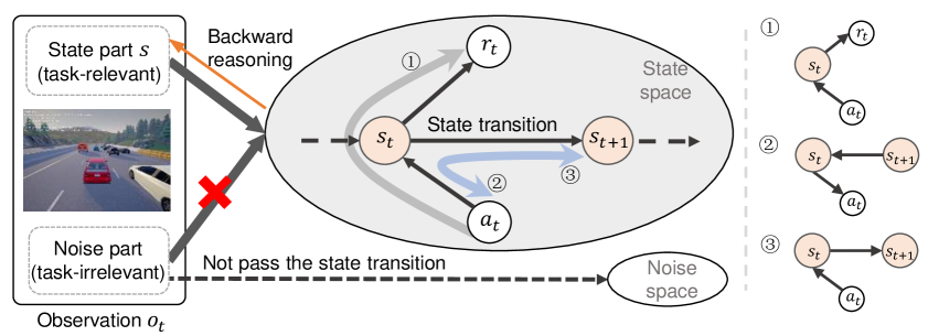
Figure 1: Task-relevant state representation derived from dynamics relationships over underlying state transition in DRL.

To refine the aforementioned concept and overcome the limitations of one-step metric predictions, DSR further introduces the sequence methods (e.g., discrete-time Fourier transform (DTFT)) with global expressive capabilities to model the reward, forward dynamics, and inverse dynamics equations. In particular, for the inverse dynamics and reward equations, we utilize the state encoder to predict the Fourier frequency domain features corresponding to the low-dimensional action and reward sequence, while minimizing the distance between the prediction and the DTFT features of true labels. This operation not only approximates the corresponding equation relationship but also aids in extracting structured features from continuous observations. For the forward dynamics equation, we introduce a latent overshooting (LO) [24] model with the capability of long-term forward prediction to minimize the distance between the multi-step predicted state and the true state label (frozen encoding state), ensuring that the encoded information adheres to the law of forward dynamics. Moreover, this procedure, in conjunction with inverse dynamics, forms a cross prediction and verification that enhances the accuracy of upstream encoded states.

DSR was initially evaluated across six tasks in the challenging Distracting DMControl (DistractingCS) Benchmark. It achieved significant overall performance improvements compared to all baselines, particularly with an average increase of 78.9% over the DrQ baseline. Further, experiments demonstrated its superior performance in real-world autonomous driving scenarios within the CARLA environment, excelling in key metrics such as driving distance and collision. Lastly, qualitative analysis through t-SNE visualization confirmed the efficient representational capacity of our method. In summary, extensive quantitative comparisons and qualitative analyses robustly demonstrate that the proposed method significantly enhanced both representational capabilities and policy performance.

Our contribution encompasses three main manifolds:

1. We propose an intrinsic dynamics characteristics-driven sequence representation method to solve the shortcomings in previous representation methods of data augmentation’s dependence on manual noise and the fact that BSM ignores the dynamic relationships between elements.

2. We introduce the DTFT transform and latent overshooting model with global expressive capabilities to further handle long-term state prediction modeling of intrinsic dynamic properties on state transitions, while extracting favorable structured features.

3. The proposed method achieves the best performance on both DistractingCS Benchmark with video background distractions and CRALA-based autonomous driving with natural visual distractions. Moreover, the qualitative analysis results strongly demonstrate the outstanding representation abilities of the method.

II Preliminaries

II-A Deep Reinforcement Learning

In our task setting, the underlying interaction between the environment and the agent is modeled as a Markov decision process (MDP), described by the tuple ${\cal M}=({\cal S},{\cal A},{\cal P},R,\gamma)$, where $\cal S$ represents the continuous state space, $\cal A$ the continuous action space, ${\cal P}(s_{t+1}|s_{t},a_{t}):{\cal S}\times{\cal A}\times{\cal S}\to[0,1]$ the probability of transitioning from state $s_{t}\in\cal{S}$ to state $s_{t+1}\in\cal{S}$ when executing an action $a_{t}\in\cal{A}$ at time $t$, $r_{t}=R(s_{t},a_{t}):{\cal S}\times{\cal A}\to\mathbb{R}^{1}\in{\cal R}$ the reward signal obtained by the agent when given the state $s_{t}$ and the action $a_{t}$, and $\gamma\in[0,1]$ the discount factor of rewards.

An agent chooses an action $a_{t}\in{\cal A}$ according to a policy function $a_{t}~{}\pi\left(\cdot|s_{t}\right)$, which updates the system state $s_{t+1}\sim{\cal P}\left(\cdot|s_{t},a_{t}\right)$, yielding a reward $r_{t}\in{\cal R}$. The agent’s optimization goal is to maximize the expected cumulative discounted rewards by learning a good policy: $\pi^{*}={\underset{\pi}{\arg\max}{\mathbb{E}_{\tau\sim(\pi,{\cal M})}\left[{\sum_{t=0}^{T-1}{\gamma^{t}r_{t}}}\right]}}$. It is worth noting that due to the fact that single image observation usually does not satisfy the full observability of systems [25], we stack three consecutive images as the current observation $o_{t}$ while training an encoder network $\phi$ to extract true state information from the observation: $\hat{s}=\phi(o_{t})$.

II-B Actor-Critic Framework

Actor Critic (AC) framework [26] is an off-policy reinforcement learning algorithm for continuous control tasks, and it is also the fundamental framework for all algorithms mentioned in this work. In general, AC consists of a critic network for learning the value function $Q_{\psi}(s_{t},a_{t})$ and an actor network for learning the policy function $\pi_{\varphi}(a_{t}|s_{t})$. Differ to the value-based methods, SAC optimizes a non-deterministic policy to maximize the expected trajectory return. Specifically, the critic network optimizes the temporal difference (TD) loss derived from the Bellman optimality equation while training the state action value function $Q_{\psi}(s_{t},a_{t})$ with parameter $\psi$ through sampling estimation [27]. The loss is defined as,

$${\cal L}{(\psi)}=\mathbb{E}_{s_{t},a_{t}\sim\cal B}\left[\frac{1}{2}\left[(r_{t}+\gamma(1-d){\cal T})-{\left(Q_{\psi}(s_{t},a_{t})\right)}^{2}\right]\right]$$ (1)

with,

$${\cal T}=\mathbb{E}_{a^{\prime},s_{t+1}\sim\cal B}\left[{\underset{a^{\prime}_{t}}{\max}}Q^{tgt}_{\hat{\psi}}(s_{t+1},a^{\prime}_{t})\right].$$ (2)

In the above formula, $Q_{\hat{\psi}}^{tgt}$ represents the target $Q$ function with frozen network parameters $\hat{\psi}$, where $\hat{\psi}$ is updated from the exponential moving average (EMA) of the trainable parameters $\psi$, $d$ indicates the “done” signal of an episode, $\mathcal{B}$ represents the experience replay buffer of the off-policy DRL.

Furthermore, we train the actor network with parameters $\varphi$ by sampling actions $a_{t}\sim\pi_{\varphi}$ from the policy and maximizing the expected reward of the sampled actions:

$$\mathcal{L}_{\pi}(\varphi,\psi)=\mathbb{E}_{a^{{}^{\prime}}\sim\pi_{\varphi},s_{t}\sim\mathcal{B}}\left[{Q^{\pi}_{\psi}\left(s_{t},a^{\prime}\right)}\right]$$ (3)

II-C Behavior Similarity Metrics

Behavior Similarity Measure (BSM) uses elements such as rewards and actions on MDP to measure task similarity between two states, with a typical representative of Bisimulation Metric [14]. Bisimulation Metric measures the equivalence relationship between two states on MDP in a recursive form, i.e., if two states share an equivalence distribution on the next equivalent state, as well as they have the same immediate reward, and then they are considered equivalent [28]. Under the guidance of this theory, existing methods usually utilize Bisimulation Metric to learn a parameterized state encoder based on distance loss of elements on MDP [29].

Our work follows the feature of using elements to learn equivalent task-relevant representations in the Bisimulation Metric, but the difference is that it adopts a prediction mode for target elements, which helps alleviate the existing problem of information consumption [17], and it is also beneficial to extend to sequence representation setting.

II-D Discrete-Time Fourier Transform

The Discrete-Time Fourier Transform (DTFT) is a powerful continuous signal processing tool that converts discrete-time signals into continuous frequency domain information. Therefore, we leverage this property to reveal the intrinsic relationship among continuous time-domain signals from a frequency domain perspective, thereby facilitating the encoder to capture global features such as periodicity and structure.

Formally, the DTFT converts a discrete real sequence ${\{x_{n}\}}_{n=-\infty}^{+\infty}$ into a frequency domain signal through a complex variable function $F(\omega)=\sum_{n=-\infty}^{\infty}{x_{n}e^{-(j\omega n)}}$, where $\omega$ is a frequency domain variable, $j$ is an imaginary unit, and $F\left(\omega\right)$ satisfies the periodic property, i.e., $F\left(\omega\right)=F\left(\omega+2k\pi\right)$. In this work, to simplify the calculation, we focus on the frequency domain signal of $\omega$ within a single period interval $[-\pi,\pi]$ that still contains all information in the infinite time domain.

III Method

In this section, we propose a sequence representation learning method (DSR) driven by intrinsic dynamics characteristics, which uses the dynamics equations related to the underlying state transition to derive complete state information from sequence observations. Since DSR only uses the inherent properties of RL itself to learn representations without resorting to contrastive noise, it can be extended to the DRL framework in image or low-dimensional vector decision-making scenarios.

The overall structure of this section is as follows: First, in Section 4.1, we will introduce the dynamics equations with inherent dynamics characteristics in the RL decision-making system and introduce a basic optimization objective. Then, in Section 4.2, we further provide sequence optimization loss in the basic optimization form and provide its implementation framework, as shown in Figure 2. For the implementation framework, we will introduce the details of DTFT modeling about the equation relationships of the inverse dynamics and the reward in Section 4.3; Finally, the multi-step prediction model used to fit the forward dynamics equation relationship is introduced in Section 4.4.

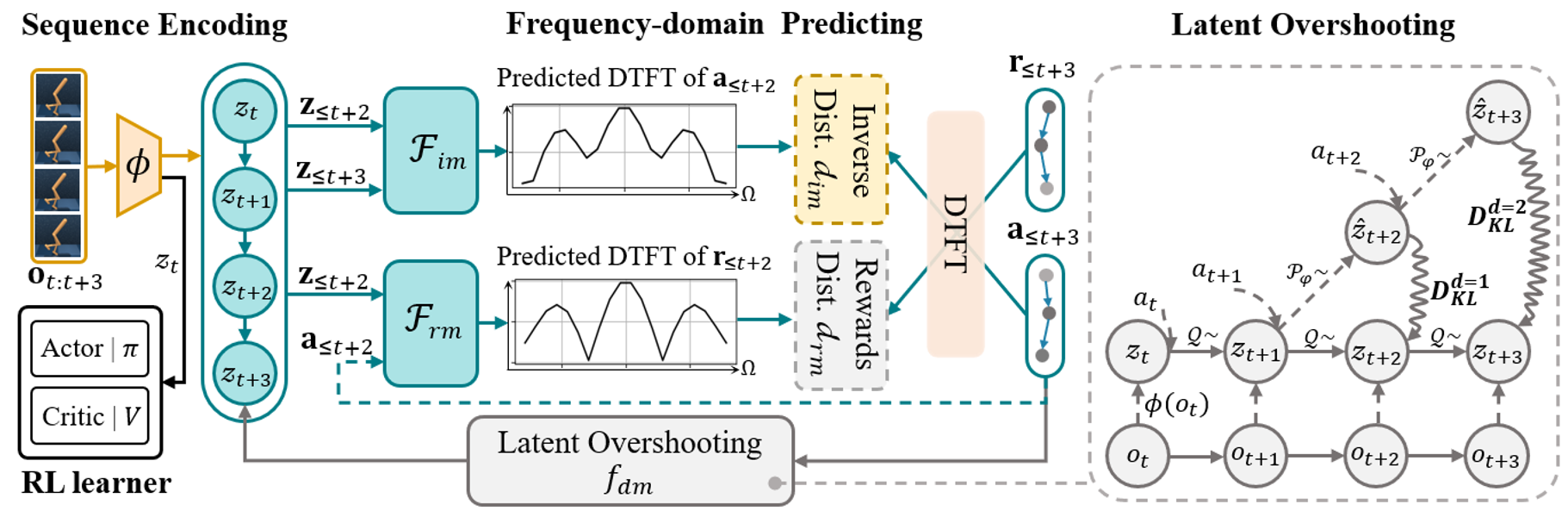
Figure 2: Overview of the DSR framework: The method is divided into four parts: sequence encoding, frequency domain prediction, latent overshooting, and reinforcement learning, with different sections distinguished by colored connection arrows. The entire framework focuses on the encoder $\phi$ as the core training target, and the trained encoder will be used for reinforcement learning policy training. In the Figure, $z_{\leq t+2}$ and $z_{\leq t+3}$ are shorthand for the sequential latent encoded states $z_{t:t+2}$ and $z_{t+1:t+3}$, respectively (similarly for other vectors).

III-A Intrinsic dynamics Characteristics

The underlying dynamics characteristics of the reinforcement learning system can be defined as a probability distribution function $T\left(s_{t+1},r_{t}\middle|s_{t},a_{t}\right):{\cal S}\times{\cal A}\times{\cal S}\times{\cal R}\rightarrow[0,1]$[22], which can be further decomposed into ①reward equation, ②inverse dynamics equation and ③forward dynamics equation maintained by reward, action and state elements (shown on the right of Figure 1):

$$\left\{\begin{matrix}\left.{}r_{t}=r\left({s_{t},a_{t}}\right),r:{\cal S}\times{\cal A}\rightarrow{\cal R}\right.\\ \left.{}a_{t}=v\left(s_{t},s_{t+1}\right),v:{\cal S}\times{\cal S}\rightarrow{\cal A}\right.\\ \left.{}s_{t+1}=p\left(s_{t},a_{t}\right),p:{\cal S}\times{\cal A}\rightarrow{\cal S}\right.\end{matrix}\right.$$ (4)

Eq. (1) describes the dynamics equation relationships established in the real states, where the functions $r$, $v$, and $p$ are respectively given by the environment. Our goal is to leverage those known relationships and sampled data to adversely derive the accurate state part from the observations with visual distractions. Therefore, we first modify Eq. (1) into the following approximate equation with observations and a parameterized encoder $\phi$:

$$\left\{\begin{matrix}\left.{}r_{t}\simeq r_{\phi}\left({z_{t},a_{t}}\right),~{}r_{\phi}:Z\times{\cal A}\rightarrow{\cal R}\right.\\ \left.{}a_{t}\simeq v_{\phi}\left(z_{t},z_{t+1}\right),v_{\phi}:Z\times Z\rightarrow{\cal A}\right.\\ \left.{}z_{t+1}\simeq p_{\phi}\left(z_{t},a_{t}\right),p_{\phi}:Z\times{\cal A}\rightarrow Z\right.\end{matrix}\right.$$ (5)

where $z_{t}\in Z$ represents the (latent) encoding state, i.e., $z_{t}=\phi(o_{t})$. Additionally, the reward $r_{\phi}$, reverse dynamics $v_{\phi}$, and forward dynamics $p_{\phi}$ are respectively modeled as prediction models with reward $r_{t}$, action $a_{t}$, and encoding state $z_{t+1}$ as self-supervised labels. Then, these models with dynamics characteristics will be integrated into the following learning objective ${\cal J}^{o}(\phi)$ in Eq . (6):

$${\cal J}^{o}(\phi)={\mathbb{E}_{o_{t},a_{t},r_{t}\sim\pi,\mathcal{M}}\left[\left({d\left({r_{\phi}\left({z_{t},a_{t}}\right),{\overset{-}{r}}_{t}}\right)\linebreak+d\left({v_{\phi}\left({z_{t},z_{t+1}}\right),{\overset{-}{a}}_{t}}\right)+d\left({p_{\phi}\left({z_{t},a_{t}}\right),{\overset{-}{z}}_{t+1}}\right)}\right)^{2}\right]}$$ (6)

$$\scriptsize{\cal J}^{seq}(\phi)=\mathbb{E}_{\mathbf{o},\mathbf{a},\mathbf{r}\sim\pi,\mathcal{M}}\left[\left({d\left({r_{\phi}\left(\mathbf{z}_{t:t+T-1},\mathbf{a}_{t:t+T-1}\right),\mathbf{r}_{t+1:t+T}}\right)+d\left({v_{\phi}\left({\mathbf{z}_{t:t+T-1},\mathbf{z}_{t+1:t+T}}\right),\mathbf{a}_{t+1:t+T}}\right)+d\left({p_{\phi}\left(\mathbf{z}_{t:t+T-1},\mathbf{a}_{t:t+T-1}\right),{\overset{-}{z}}_{t+T}}\right)}\right)^{2}\right]$$ (7)

In Eq. (6), the $d$ represents some distance metrics, and the self-supervised label ${\bar{z}}_{t+1}$ is a frozen encoding state, which uses bootstrapping to simultaneously improve the label accuracy and encoder parameters.

III-B Sequential Optimization Objective

In the previous section, we introduced a basic optimization objective that incorporates dynamics characteristics. While it can be directly optimized, its single-step distance cannot effectively distinguish between two similar tasks/behaviors in observations. Especially in scenarios with sparse targets, this problem will be exacerbated [22]. According to this suggestion, we modify the original optimization objective ${\cal J}^{o}(\phi)$ into a multi-step optimization loss objective, defined in as ${\cal J}^{seq}(\phi)$ in Eq. (7).

On the other hand, Theorem 2 in the work [30] demonstrated the existence of favorable periodic and highly structured timing-related features in sequence states. Inspired by this, while fitting the dynamics equation relationships from a sequence optimization perspective (Eq. (7)), we can also deeply model the self-supervised labels with continuous property to promote the encoder to learn the above-mentioned temporal features.

Consequently, to further obtain such global temporal features, we utilize some sequence methods to model the potential relationships within the self-supervised labels, rather than naively optimizing the original distances (e.g., element error) in the sequence objective over Eq. (7). Specifically, we introduce the Discrete Time Fourier Transform (DTFT) to obtain the frequency domain signals of action sequences $\mathbf{a}_{t+1:t+T}\in\mathbb{R}^{T\times d1}$ and reward sequences $\mathbf{r}_{t+1:t+T}\in\mathbb{R}^{T\times 1}$ in the T dimension, where $d1$ and $T$ are the action dimension and sequence length respectively. In addition, for high-dimensional ${\bar{z}}_{t+T}\in\mathbb{R}^{d2}$ ($d2$ is the dimension of the encoding state), we utilize a latent overshooting model that satisfies the forward dynamics equation to minimize the Kullback-Leibler (KL) divergence between the multi-step state prediction and the real state distribution. Final, we minimize the following final loss:

$$\mathcal{L}(\phi)=d_{rm}\left({\mathcal{F}_{rm}^{\phi}\left({\mathbf{z}_{t:t+T-1},\mathbf{a}_{t:t+T-1}}\right),F\left(\mathbf{r}_{t+1:t+T}\right)}\right)$$

$$+d_{im}\left({\mathcal{F}_{im}^{\phi}\left({\mathbf{z}_{t:t+T-1},\mathbf{z}_{t+1:t+T}}\right),F\left(\mathbf{a}_{t+1:t+T}\right)}\right)+D_{KL}\left[p_{\phi}\middle||q]\right.$$ (8)

Where the $\mathcal{F}_{rm}^{\phi}$ and $\mathcal{F}_{im}^{\phi}$ represent the Fourier prediction models for the reward and inverse dynamics equations respectively, $F$ denotes the Fourier transform of the sequence target, $p_{\phi}\left(z_{t+T}\middle|\mathbf{o}_{t:t+T-1},\mathbf{a}_{t:t+T-1}\right)$ represents the probability distribution of the predicted multi-step states, $q\left(z_{t+T}\middle|\mathbf{o}_{t:t+T-1},\mathbf{a}_{t:t+T-1}\right)$ represents the true state distribution probability, and subscripts ”rm” and ”im” represent the reward model and the inverse dynamic model, respectively

Finally, as shown in Figure 2, our method presents an optimization framework constrained by the underlying reward, inverse dynamics, and forward dynamics equations, based on the final sequence optimization objective in Eq. (III-B). The modeling details of the DTFT frequency domain prediction model and the multi-step state prediction are discussed in the following two sections.

III-C Prediction of DTFT

This section of the method fits the inverse dynamics equations and reward equations related to underlying state transitions from the DTFT frequency domain perspective of sequential actions $\mathbf{a}_{t+1:t+T}$ and rewards $\mathbf{r}_{t+1:t+T}$. The following details the DTFT transformation and prediction process using sequential actions as an example, with the procedure for sequential rewards being identical.

First, since the frequency domain period of the discrete-time action signal is $2\pi$, we only consider the DTFT over a single period $[-\pi,\pi]$. The following equation represents the complex-valued function $F_{\mathbf{a}}\left(\mathbf{\omega}\right)$ for the frequency variable $\mathbf{\omega}$ in the DTFT of the sequence action target:

$$F_{\mathbf{a}}\left(\mathbf{\omega}\right)={\sum_{n=t+1}^{t+T}{a_{n}e^{-in\mathbf{\omega}},}}\mathbf{\omega}\in[-\pi,\pi]$$ (9)

where $\mathbf{\omega}\in\mathbb{R}^{k}$ is a list of frequencies sampled evenly $k$ times over the interval $[-\pi,\pi]$, where $k=20$.

$$\min f_{dm}={{D_{KL}\left[p_{\phi}\middle|\middle|q\right]}}={{ELBO\left(\mathbf{o}_{t:t+T-1},\mathbf{a}_{t:t+T-1}\right)}}$$

$$=\mathbb{E}_{z_{t+T}\sim p_{\phi}}\underset{reconstruction}{\underbrace{\left[{logq_{\theta}\left({\mathbf{o}_{t:t+T-1},\mathbf{a}_{t:t+T-1}}\right)}\right]}}-\delta_{\pi,t}D_{KL}\underset{multi-step~{}prediction}{\underbrace{\left[p_{\phi}\left(z_{t+T}\middle|{\mathbf{o}_{t:t+T-1},\mathbf{a}_{t:t+T-1}}\right)\middle|\middle|q_{\theta}\left(z_{t+T}\middle|\mathbf{o}_{t:t+T-1},\mathbf{a}_{t:t+T-1}\right)\right]}}$$ (10)

In practice, the amplitude $\Gamma_{Amp}F_{\mathbf{a}}\in\mathbb{R}^{1\times k}$ and phase $\Gamma_{Pha}F_{\mathbf{a}}\in\mathbb{R}^{1\times k}$ of the action’s DTFT are used as self-supervised targets, defined as follows:

$$\Gamma_{Amp}F_{\mathbf{a}}=\left|{F_{\mathbf{a}}(\omega)}\right|,~{}\Gamma_{Pha}F_{\mathbf{a}}=arctan\frac{Im\left(F_{\mathbf{a}}(\omega)\right)}{Re\left(F_{\mathbf{a}}(\omega)\right)}$$ (11)

For the Fourier prediction model, based on the settings of the inverse dynamics Eq. (5), we use the adjacent sequence encodings $(\mathbf{z}_{t:t+T-1},\mathbf{z}_{t+1:t+T})$ as an input to the inverse dynamics parametric model $f_{\phi}\in\mathbb{R}^{2\times k}$, denoted by $\mathcal{F}_{im}$ as follows:

$$\small\mathcal{F}_{im}\left({\mathbf{z}_{t:t+T-1},\mathbf{z}_{t+1:t+T}}\right)=f_{\phi}\left({agg\left({\phi\left(\mathbf{o}_{t:t+T-1}\right),\phi\left(\mathbf{o}_{t+1:t+T}\right)}\right)}\right)$$ (12)

Ultimately, by integrating the aforementioned DTFT target $F_{\mathbf{a}}$ and the prediction model $\mathcal{F}_{im}$, we optimize both the amplitude distance and phase distances of the sequence actions to ensure the inverse dynamics process:

$$d_{im}\left({\mathcal{F}_{im}\left({\mathbf{z}_{t:t+T-1},\mathbf{z}_{t+1:t+T}}\right),F\left(\mathbf{a}_{t+1:t+T}\right)}\right)$$

$$=\mathbb{E}_{a\sim\pi,s\sim P}\left[{\left\|{\Gamma_{Amp}\mathcal{F}_{im}-\Gamma_{Amp}F_{\mathbf{a}}}\right\|+\left\|{\Gamma_{Pha}\mathcal{F}_{im}-\Gamma_{Pha}F_{\mathbf{a}}}\right\|}\right]$$ (13)

Similarly, we can derive the optimization loss for the reward prediction model, which targets the DTFT features of the sequence rewards:

$$d_{rm}\left({\mathcal{F}_{rm}\left(\mathbf{z}_{t:t+T-1},\mathbf{a}_{t:t+T-1}\right),F\left(\mathbf{r}_{t+1:t+T}\right)}\right)$$

$$=\mathbb{E}_{a\sim\pi,s\sim P,r\sim R}\left[{\left\|{\Gamma_{Amp}\mathcal{F}_{rm}-\Gamma_{Amp}F_{\mathbf{r}}}\right\|+\left\|{\Gamma_{Pha}\mathcal{F}_{rm}-\Gamma_{Pha}F_{\mathbf{r}}}\right\|}\right]$$ (14)

III-D Forward dynamics

To learn a latent encoding state that complies with the forward eqution with underlying continuous state transition rules, we introduce a long-term forward dynamics model based on multi-step planning, known as Latent Overshooting [24], as shown on the right side of Figure 2. Overall, LO uses a two-level planner to better understand the dynamics transition process through long-term behaviors, while fitting a state transition model with long-term predictive accuracy, encouraging the encoder to extract task-relevant information about dynamics.

The above optimization problem can be characterized as minimizing the KL divergence between the multi-step latent state transition distribution $p_{\phi}\left(z_{t+T}\middle|\mathbf{o}_{t:t+T-1},\mathbf{a}_{t:t+T-1}\right)$ and the true state distribution $q\left(z_{t+T}\middle|\mathbf{o}_{t:t+T-1},\mathbf{a}_{t:t+T-1}\right)$, denoted as $D_{KL}\left[p_{\phi}||q\right]$. However, as the original KL distance includes the intractable true distribution $q$, we use variational inference to transform this challenging problem into a parameterized gradient optimization problem. For this, we first present the following theory:

Theorem 1

Let the sequence observation data be represented by $\mathbf{o}_{t:t+T-1}$ and $\mathbf{a}_{t:t+T-1}$, and given the approximate posterior $p_{\phi}$ with the encoding parameters $\phi$, the evidence lower bound (ELBO) on the data log-likelihood is:

$$logq\left({\mathbf{o}_{t:t+T-1},\mathbf{a}_{t:t+T-1}}\right)$$

$$={\int{p_{\phi}\left(z_{t+T}\middle|{\mathbf{o}_{t:t+T-1},\mathbf{a}_{t:t+T-1}}\right)logq\left({\mathbf{o}_{t:t+T-1},\mathbf{a}_{t:t+T-1}}\right)dz_{t+T}}}$$

$$=\mathbb{E}_{z_{t+T}\sim p_{\phi}}log\frac{q\left({z_{t+T},\mathbf{o}_{t:t+T-1},\mathbf{a}_{t:t+T-1}}\right)}{p_{\phi}\left(z_{t+T}\middle|{\mathbf{o}_{t:t+T-1},\mathbf{a}_{t:t+T-1}}\right)}+\mathbb{E}_{z_{t+T}\sim p_{\phi}}D_{KL}\left[p_{\phi}\middle|\middle|q\right]$$

$$\geq\mathbb{E}_{z_{t+T}\sim p_{\phi}}log\frac{q\left({z_{t+T},\mathbf{o}_{t:t+T-1},\mathbf{a}_{t:t+T-1}}\right)}{p_{\phi}\left(z_{t+T}\middle|{\mathbf{o}_{t:t+T-1},\mathbf{a}_{t:t+T-1}}\right)}$$

$$\triangleq ELBO\left({\mathbf{o}_{t:t+T-1},\mathbf{a}_{t:t+T-1}}\right)$$ (15)

Proof:

The proof can be seen in Appendix A1. ∎

Based on this conclusion, since the evidence probability $logq\left(\mathbf{o}_{t:t+T-1},\mathbf{a}_{t:t+T-1}\right)$ remains constant during the optimization of the posterior $p_{\phi}$, minimizing the original objective $D_{KL}\left[p_{\phi}||q\right]$ is equivalent to maximizing the $ELBO\left(\mathbf{o}_{t:t+T-1},\mathbf{a}_{t:t+T-1}\right)$. Hence, we can further derive the objective in Eq. (III-C).

The derivation of Eq. (III-C) is shown in Eq (A2. Supplement for Section Forward Dynamics) of Appendix A2. Ultimately, the original challenging is transformed into a gradient-optimizable problem, involving the KL loss between the priors associated with encoding parameters $\phi$ and reconstruction parameters $\theta$, and a reconstruction loss term related to $\theta$.

It is important to note that in the early stages of training, using the imprecise latent state ${\bar{z}}_{t+T}$ as the self-supervised target for the forward dynamics model $p_{\phi}\left(z_{t+T}\middle|\mathbf{o}_{t:t+T-1},\mathbf{a}_{t:t+T-1}\right)$ can lead to instability in representation learning. To this end, we have incorporated an adaptive factor $\delta_{\pi,t}$ into our derived final objective in Eq. (III-C) to reduce the early influence of the forward dynamics term on overall representation learning, calculated as follows:

$$\delta_{\pi,t}=min\left({\rho_{\pi,t},clip\left({\rho_{\pi,t},1-\epsilon,1+\epsilon}\right)}\right)$$ (16)

with,

$$\rho_{\pi,t}=\frac{1}{\left|\mathcal{A}\right|}{\sum_{i=1}^{|\mathcal{A}|}\left|\frac{c}{\pi_{\theta+\mathrm{\Delta}\theta}^{(i)}\left(z_{t}\right)-\pi_{\theta}^{(i)}\left(z_{t}\right)}\right|}$$ (17)

To obtain the factor $\delta_{\pi,t}$ at time $t$, we first need to calculate the average difference $\rho_{\pi,t}$ between the current policy $\pi_{\theta+\mathrm{\Delta}\theta}^{(i)}\left(z_{t}\right)$ and the old policy $\pi_{\theta}^{\left(i\right)}\left(z_{t}\right)$ under the same current encoding state $z_{t}$, where $c$ is a scaling hyperparameter. Additionally, to keep it within a reasonable positive range, we use the clip function to trim $\rho_{\pi,t}$. Overall, the contribution of the forward dynamics terms to the overall representation learning increases as the policy improves.

Algorithm 1 Intrinsic Dynamic Characteristics-driven Sequence Representation learning DRL method

Input: replay buffer $D$ with size $N$, videos dataset $\cal X$, learning rate, batch size, etc.
Output: optimal $\pi$

1:  Initialize Critic network $\varphi$, Actor network $\psi$, and encoder network $\phi$.

2:  for episode $m\leftarrow 0$ to $M$ do

3:     Initial observation $o_{t}$.

4:     Encode state: $z_{t}=\phi(o_{t})$.

5:     Cumpute action: $a_{t}=\pi(\cdot|z_{t})$.

6:     Excute an interaction: $o_{t},a_{t},r_{t+1},done=Env(a_{t})$.

7:     Collect data $D\leftarrow D\cup\{o_{t},a_{t},r_{t+1},done\}$.

8:  end for

9:  for gradient step $i\leftarrow 0$ to $I$ do

10:     Get sequence $\{a_{i:i+T-1},r_{i:i+T-1},o_{i:i+T-1}\}$ from $D$.

11:     Transform action sequence by DTFT in Eq. (11).

12:     Transform reward sequence by DTFT in Eq. (11).

13:     Compute the objectives of $d_{im}$, $d_{rm}$ and $f_{dm}$.

14:     Train the Actor-Critic ${\cal L}_{Q}+{\cal L}_{\pi}$. (Eq. (1) and Eq. (3)).

15:     Train the auxiliary task ${\cal L}=d_{im}+d_{rm}+f_{dm}$. (Eq. (8)).

16:  end for

17:  return optimal $\pi$

IV Experiments

To test the representation ability and policy performance of the DSR method, we conduct standardized evaluations on six continuous control tasks on the challenging visual Distracting DeepMind Control Suite benchmark (DMControl) [31]. To further verify the superiority of DSR, we applied it to the real-world CARLA-v0.98 autonomous driving simulation environment [32]. In the whole experiment, DSR is compared with a series of recent representation learning-related DRL baselines that perform strongly on the Distracting DMControl benchmark. In addition, we also qualitatively discussed the generalization ability of DSR to task-relevant information in visual tasks by the results of t-SNE visualization. It is worth noting that the DSR can be embedded into a variety of visual reinforcement learning frameworks as an efficient plug-in, and it is extended to the DrQ algorithm [8] in this work. Therefore, one focus of the experiments is the performance improvement produced by inserting the DSR method into the DrQ.

Baselines The DrQ-based DSR method (also denoted as DrQ+ DSR) takes advantage of the inherent dynamics transition properties underlying reinforcement learning to learn representations. Therefore, we first compared the recent DrQ algorithm [8], which achieves SOTA performance on the clean DMControl benchmark through regularized Q function. As a comparison regarding dynamics representation, we compare the PAD algorithm [33], which achieves superior generalization performance using a forward dynamics model. Finally, we compared the common CURL [12], which primordially introduced contrastive representation learning into visual DRL, while achieving the best performance on the DMControl benchmark.

IV-A Evaluation on the Distracting Control Suite

Distracting DeepMind Control Suite Setting Distracting DMControl suite is a hard setting with video background distracting grounded in the DeepMind Control Suite continuous control task [34], which has been widely used in visual DRL to test the performance of state representation and scene generalization. Following the settings of existing work [31][35], the distracting DMControl suite replaces the clean background with natural video sampled from the DAVIS 2017 dataset [36] as the noise of the observations. Furthermore, to verify the generalization ability of the method in unseen scenes, it is trained in two fixed distracting videos, but evaluated on arbitrary scenes among 30 unseen distracting videos.

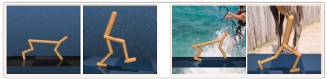
Figure 3: Visual task examples for cheetah_run and walker_walk. Left: clean DMControl setting with original background; Right: distracting DMControl setting with random background videos. Among them, the cheetah_run task is to control the six-degree-of-freedom cheetah robot to run rapidly.; the walker_walk task is to control the six-degree-of-freedom humanoid robot to walk rapidly.

Hyperparameter Setting We use the same hyperparameter settings and the network architecture for DSR and baselines. Specifically, the training observations are stacked by three sequential RGB frames with the shape $9\times 84\times 84$. The observation encoder consists of a 4-layer convolutional network with 32 filters and a 2-layer fully connected network with 1024 units, and the final dimension of state representation used for decision-making is 50. In addition, we set the capacity of the replay buffer to 1e5, the minibatch size to 256, the initial temperature coefficient to 0.1, and employ the Adam optimizer with a learning rate of 5e-4 to optimize the critic, actor, and encoder networks. For the individual DSR representation task, we set the sequence length of MDP elements to 3, the sample number of the DTFT period to 20, and the minibatch of the auxiliary training to 256. Detailed parameters are shown in Table 2.

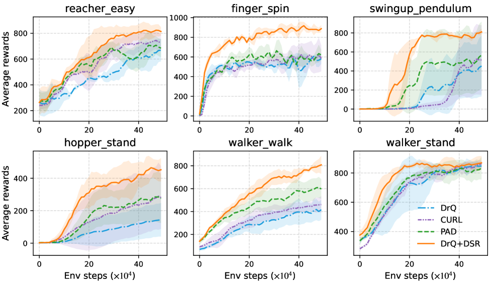
Figure 4: Evaluation curves on distracting DMControl suite with unseen video background setting at 500K environment steps. For each method, the results are derived from the mean rewards and standard deviation of 3 random seed experiments. A total of 50 evaluations were completed for each experiment, where the checkpoint score for each evaluation was averaged over 10 episodes. The yellow line (DrQ+DSR) is our method.

Methods	Reacher_easy	Finger_spin	Swingup_pendulum	Hopper_stand	Walker_walk	Walker_stand
DrQ	668.5$\pm$86	606.3$\pm$7	452.4$\pm$320	143.8$\pm$103	418.0$\pm$93	847.9$\pm$22
CURL	745.0$\pm$68	623.3$\pm$119	524.6$\pm$370	289.3$\pm$207	461.2$\pm$73	863.0$\pm$20
PAD	707.7$\pm$69	664.0$\pm$67	567.1$\pm$352	284.7$\pm$152	610.8$\pm$92	832.9$\pm$77
DSR (ours)	824.0$\pm$46	917.9$\pm$138	811.1$\pm$33	464.7$\pm$63	808.4$\pm$79	869.3$\pm$47
vs. DrQ	$\left.\uparrow 23.3\mathbf{\%}\right.$	$\left.\uparrow 51.4\mathbf{\%}\right.$	$\left.\uparrow 79.3\mathbf{\%}\right.$	$\left.\uparrow 223.2\mathbf{\%}\right.$	$\left.\uparrow 93.4\mathbf{\%}\right.$	$\left.\uparrow 2.5\mathbf{\%}\right.$

TABLE I: The best mean episode rewards on distracting DMControl suite with unseen video background setting at 500K environment steps. We report the mean and standard deviation of three repeated experiments, as well as the improvement percentage of DSR compared to the backbone DrQ.)

Figure 5: Training curves of our method (DrQ+DSR) and DrQ backbone on two seen background videos.

Main Results As depicted in Figure 4, we report the evaluation results of DSR compared to the recent DrQ, CURL, and PAD on 6 tasks of reacher_easy, finger_spin, swingup_pendulum, hopper_stand, walker_walk and waker_stand over the process of training. All experiments used 30 unseen background videos for visual distraction (demonstrated in Figure 3) during the evaluation stage. As a result, the proposed DSR (DSR+DrQ) method achieves significant performance improvements in all tasks compared to all baselines, especially compared to the DrQ backbone, which averaged 78.9%. In addition to the best rewards, DSR also converged faster in comparison to all baselines. Intuitively, the comparative results powerfully demonstrate that DSR has learned task-relevant state information during the training process, so that it is able to execute background-independent policies in unseen scenarios, and then achieves the best policy performance. Notably, the swingup_pendulum and hopper_stand are sparse reward tasks with few dense reward signals, which wreaks havoc on both policy and representation learning. Nevertheless, the DSR method still improves 79.3% and 223.2% compared to the DrQ, as shown in Table 1.

As mentioned above, evaluation results show that our method improves DrQ’s abilities in both task-relevant representation and generalization to unknown scenes/videos, yet the abilities need to be learned and acquired during training. To further demonstrate the learning ability of the DSR, we provide a separate comparison between DSR and DrQ in the training process in Figure 5. We can clearly observe that once DSR is inserted into DrQ, the proposed DrQ+DSR method greatly improves the overall performance of the original DrQ in terms of convergence speed and optimal rewards on 6 visual tasks.

Figure 6: t-SNE visualizations of the latent encoding spaces learned with the DSR encoder (left t-SNE result) and DrQ encoder (right t-SNE result). Each observation image points to positions (higher value yellow, lower value purple) under the two encoding spaces through the corresponding arrow.

Qualitative Analysis To qualitatively analyze the representation ability of the encoder, we employ t-SNE visualization to illustrate that DSR can encode observation images with similar behaviors/tasks into close coordinate distances, achieving the extraction of invariant representations independent of background distractions. In this experiment, we use t-SNE to project the encoding state of batch observations under the DSR or DrQ encoder space into a two-dimensional space and then embed them into Cartesian coordinates. In addition, we also use the learned state value to render the color of each coordinate point. Therefore, the position of each coordinate point represents the encoded information of an observation, and the color depth represents the value of the observation.

As shown in Figure 6, the two sides are the t-SNE embedding plots of the same batch of observation images under the DSR and DrQ encoders respectively, and the middle is two arbitrary observation groups with similar tasks in the batch. From the figure, we can easily see that, i) for each observation group, although the background noise between observations is very different, their coordinate distances (left) in the DSR encoding space are very close. However, they are far apart in the DrQ encoding space (right). This result intuitively shows that it is precisely because the encoder trained by DSR can extract task-relevant information more accurately than DrQ that it can encode the observation group with similar tasks into a very close distance. ii) By observing the color of the embedding position, we also find that similar tasks/behaviors encoded by DSR have similar values, showing consistently high values for good behaviors (upper group) and low values for unfavorable behaviors (lower group). Instead, this is not entirely consistent in the DrQ embedding plot. The comparative result shows that our method can learn a more accurate state value function that is beneficial to policy learning.

Compared with existing work [14, 18], our task setting is more difficult. Specifically, the previous methods reset to a fixed starting position for each training episode, i.e., the yellow triangle position in the aerial view, which greatly limits the effective driving scenario. In our setting, the starting points are randomly sampled from about 100 spawn points (triangular positions) distributed throughout the map, which can effectively test the agent’s generalization ability to diverse scenarios. Another difference is that the training observation of DSR is only composed of three cameras on the vehicle’s roof, which is a 180° wide-angle RGB image with a size of $3\times 84\times 252$ pixels. Other settings are consistent with existing work. For example, the reward is set to $\left.r_{t}\left({s,a}\right)=v^{T}\hat{\mathbf{u}}*\mathrm{\Delta}t-C_{i}*impulse-C_{s}*\middle|steer\right|$ represents the effective speed of the vehicle projected onto the highway, impulse is the impact force ($N/s$) obtained by sensors, and —steer— is the amplitude of each direction control.

IV-B Verification on the Autonomous Driving

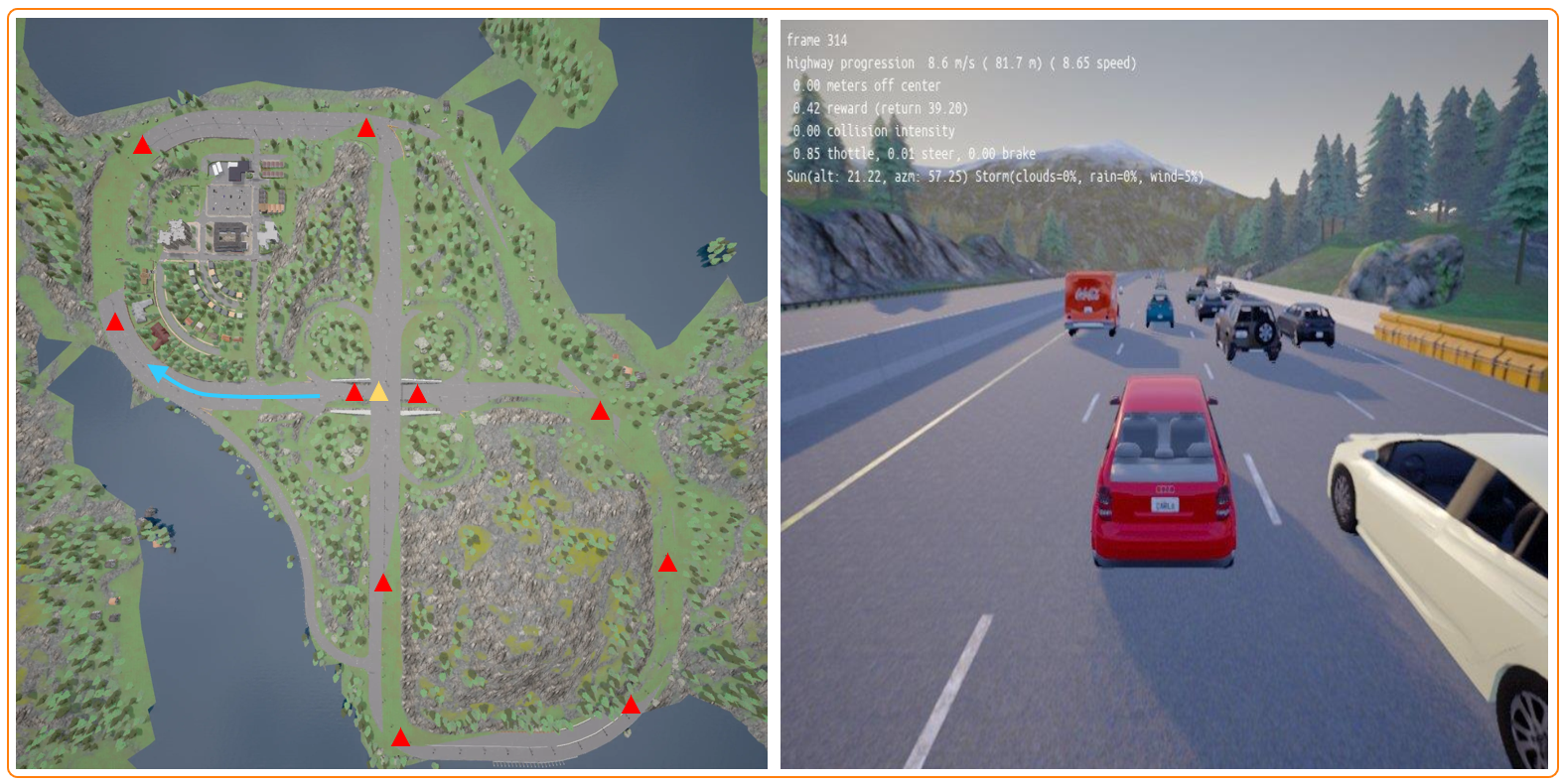
Figure 7: Left: An aerial view of the Town04 map, in which triangles represent some of the officially provided spawn points, and the blue arrow represents the driving direction; Right: A live photo, in which the red vehicle in the center is the trained agent and the others are NPC vehicles.

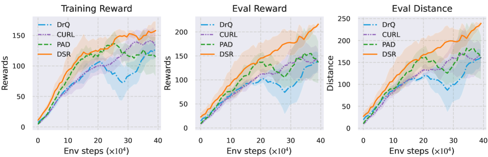
Figure 8: Experimental results of methods in the CARLA driving environment at 400K environment steps. We report the average and standard deviation of each method under three random seeds.

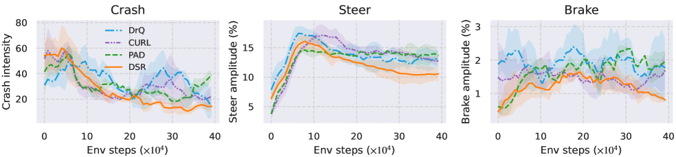
Figure 9: Comparison of key performance metrics over the training process in the CARLA driving environment.

Methods	Distance	Eval-Reward	Train-Reward	Mean Crash (N/s)	Mean Steer(%)	Mean Brake (%)
DrQ	161.3$\pm$18	138.8$\pm$18	128.1$\pm$15	13.5$\pm$8	12.2$\pm$0.5	1.5$\pm$0.4
CURL	170.9$\pm$59	147.5$\pm$50	141.8$\pm$18	19.8$\pm$1	12.7$\pm$0.7	1.1$\pm$0.3
PAD	182.3$\pm$59	155.7$\pm$53	136.4$\pm$18	18.1$\pm$3	13.4$\pm$1.6	1.4$\pm$0.5
DSR (ours)	239.1$\pm$5	216.0$\pm$6	158.0$\pm$15	10.6$\pm$3	10.4$\pm$1.4	0.8$\pm$0.1
vs. best scores	$\left.\uparrow 31.2\mathbf{\%}\right.$	$\left.\uparrow 38.7\mathbf{\%}\right.$	$\left.\uparrow 11.4\mathbf{\%}\right.$

TABLE II: Comparison of best episode scores in the CARLA driving environment. We recorded the highest scores for the first three items and the lowest scores for the last three items (at convergence).

To further verify the representation ability and policy performance of DSR in natural scenes, we test the experiment on CARLA, a hyper-realistic autonomous driving simulator environment that simulates various real components and natural phenomena. According to existing work, the experiments are implemented on the Town04 map in the CARLA simulator. Our goal is to use first-person visual images as observations to learn a driving policy that can control the vehicle to travel the longest distance. Since the driving scene contains a large number of task-irrelevant elements (e.g. mountains, clouds, and rain), as well as task-relevant feature information (e.g. roads, vehicles, and obstacles), this requires the agent to be able to learn an invariant generalization representation space.

Main Results. Figure 8 shows the main comparison results on the driving task. Specifically, we report the learning curves for the average episode reward (left), the evaluation curves corresponding to the average episode reward evaluated at every 10k step interval (center), and the evaluation curves to the average episode distance (right). The results show that, although the starting points are expanded to the entire Town04 map, our DSR method still achieves the best reward and distance in both the training and the evaluation process. Especially during the evaluation process, the driving distance of DSR is 31.2% higher than the best baseline with a clear advantage, as shown in Table 3.

In addition, we also recorded the data changes of the collision, steering, and braking performance metrics related to driving agents with the policy learning process, as shown in Figure 9. It is worth noting that our reward function is set with the goal of encouraging the agents to drive longer distances. However, all agents collectively learned to reasonably control the magnitude of each steering wheel and brake operation while reducing collisions. More importantly, as shown in Figure 9 and Table 3, the proposed method achieved the smallest average collision force, and the most reasonable direction and braking control scheme after the policy converges. In Table 3, ”Steer” and ”Brake” respectively represent the percentage of the direction angle amplitude and the percentage of the braking amplitude controlled by each action step.

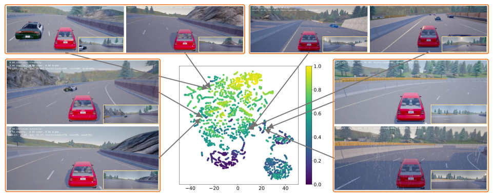
Figure 10: t-SNE visualization of the latent encoding space learned with our DSR encoder in the CARLA driving task. The red vehicles in the live photos are the trained driving agents, and the insets on the lower right are the training observations synthesized by the first-person perspective cameras.

Qualitative Analysis. To verify the ability of DSR to encode task information in the real world, we still used t-SNE to visualize the encoding distance of a batch of high-dimensional image observations under the DSR encoding space, as shown in Figure 10. The center of Figure 10 is the two-dimensional embedding plot of a batch of observations in the encoding space, and the periphery is four groups of observations with similar tasks/behaviors but large differences in natural backgrounds.

It is easy to observe that for the observation groups with very similar task information (e.g., lower right: dangerous sharp right turn; upper left: off-right turn), our DSR encoder can still encode each group to a very close distance, even though the natural backgrounds of each group are very different (e.g., lower right: bright sunny day vs. dim rainy day; upper left: trees and other vehicles vs. mountains). The result strongly demonstrates that the DSR encoder can still accurately extract task-relevant information even in complex natural backgrounds. Furthermore, this capability can promote the generalization for natural scenes and even solve some unseen risk corner cases in visual autonomous driving.

V Related Work

Visual Reinforcement Learning.  An important challenge in visual reinforcement learning is how to learn generalized representations based on image inputs [37]. Previous work has made significant efforts in this area, such as early focuses on end-to-end Attention [38] and Transformer [3] representation learning. Their basic principle relies on the reinforcement learning loss to train a task-relevant feature weight map, thereby extracting key features from the original image [39]. However, end-to-end representations that share a single reinforcement learning loss are prone to gradient vanishing issues during backpropagation, leading to insufficient representation learning ability [12]. Recently, many studies have focused on auxiliary representations, such as constructing an independent self-supervised loss through contrastive learning [40], encoding reconstruction [41], attention mechanisms [42], or behavior similarity metric [43]. Its advantage is that more complex and effective representation learning tasks can be designed without interfering with the gradient propagation of reinforcement learning itself [12]. In this work, we utilize state transition relationships to construct an auxiliary representation learning loss to learn an efficient encoder.

Data Augmentation Representations.  Data augmentation typically involves operations such as rotation, random cropping, random masking, and random PaResize on observational images [6, 13], enriching data diversity while combining specific methods to achieve effective feature representations [44, 14]. For example, in previous work, contrastive representation methods combined with data augmentation use InfoNCE loss to maximize the mutual information between an anchor and its augmented positive samples, while minimizing the mutual information between the anchor and negative samples to learn invariant representations of the augmented samples [45]. However, most contrastive representation methods are limited to using random negative samples [46], which lacks a mechanism to select negative samples that contain task-relevant information, thus limiting their representation ability in complex visual scenes [47]. Additionally, data augmentation is often used to improve their evaluation variance by regularizing Q-functions [8], eliminate task-irrelevant gradient information by balancing the Q-learning gradients of augmented samples [7], and achieve an understanding of dynamics features by pixel-level or vector-level reconstruction [41, 48]. Nevertheless, most data augmentation work relies on predefined image augmentation operations, while we cannot design infinite augmentation paradigms for real-world scenarios. Moreover, since the augmentation operations in some scenarios do not fully satisfy information invariance, it is hard to achieve an effective representation learning. In contrast, our method utilizes state transition relationships for representation learning, which can avoid the aforementioned issues.

Metric-based Representations.  Behavior Similarity Metric (BSM) methods are based on bisimulation theory [49], which employ elements such as actions on MDP collected from DRL interactions, to measure and extract equivalent task information from noisy observations [28]. Because these methods leverage the intrinsic properties of reinforcement learning to learn representations without relying on additional knowledge, they have been widely studied recently [50]. DBC is an earlier BSM method that uses reward and state transition distances to extract task-relevant information [14], but its strict distance measures can over-optimize the encoder, potentially losing beneficial information [17]. To address this, Castro et al. and Chen et al. proposed relaxed bisimulation metrics, MICO [51] and RAP distance [18], respectively, which significantly improved optimization efficiency based on bisimulation theory. Additionally, some studies suggest using actions [47], rewards [30], and other interpretable combinations [52, 53] to extract equivalent task-relevant information, even for skill sets [54]. However, most of these methods are limited to one-step distance, which makes they difficult to infer different task information at similar element distances [22]. To address these issues, we introduced sequence modeling methods to strongly identify similar one-step task/behavior information. Additionally, to improve the optimization of our objective, we use a self-supervised prediction mode instead of differential distance [47] of elements.

Multi-step Representations.  Although multi-step prediction representations can encode single-step task information more accurately, learning beneficial features through long-term prediction is challenging due to the difficulty of learning an accurate long-term prediction model [30]. To address this, further work models characteristic functions of rewards or action distributions in high-dimensional spaces [35, 47] to learn potential global structured features. Additionally, some work uses frequency domain features of reward or discounted state transitions [30][55][56] as auxiliary objectives to accelerate the extraction of potential temporal representations. In model-based deep reinforcement learning, Hafner et al. introduced Latent Overshooting, a multi-step state prediction technique that optimizes a sequential VAE [57] to enhance the model’s understanding of forward dynamics [24]. However, multi-step prediction rarely focuses on the interrelationships between different elements (e.g., the relationships between action and reward on MDP), instead calculating distances derived from each element independently, making it difficult for the encoder to leverage constraints between elements to extract more accurate states. Therefore, our method not only leverages the underlying dynamics transition relationships among different elements but also introduces useful sequence modeling methods to constrain encoder training.

VI Conclusion

We proposed a sequential representation learning method by modeling the state transition relationships (DSR) and extended it to the general DrQ deep reinforcement learning framework. The method leverages the underlying state transition rules of the system, i.e., driven by the action, the state information existing in the observation spontaneously transitions to the next state and receives the corresponding reward, whereas irrelevant non-state information typically does not satisfy this transition, thereby efficiently decomposing task-relevant state information and noise from observations. To further achieve the above motivation, we introduce various sequential models to separately model the reward, inverse dynamics, and forward dynamics equations related to state transitions, thereby constraining the optimization of the state encoder to extract information that complies with state transition rules.

DSR was first evaluated on six tasks in the challenging Distracting DMControl benchmark, showing the best performance and especially an average improvement of 78.9% over backbone baseline, while also achieving the best performance in evaluations on the real-world autonomous driving CARLA environment with natural noise. Additionally, qualitative analysis results from t-SNE visualization on the DMC and CARLA tasks confirmed that the DSR method has more efficient representation capabilities compared to the baselines. In summary, our experiments demonstrate that the proposed method significantly improves representation capabilities and policy performance. Finally, DSR can be extended as an efficient plugin to any deep reinforcement learning framework.

A3. Parameters on Distracting DMControl and CARLA tasks

TABLE III: Partial hyperparameters used for experiments of CARLA tasks

Hyperparameter	Value
Camera number	3
Full fov angles	3$\times$60 degree
Observation downsampling	84 $\times$ 252
Initial exploration steps	100
Training frames	400000
Action repeat	4
Batch size	64
$\Delta t$	0.05 seconds
$C_{i}$	0.0001
$C_{s}$	1.0

TABLE IV: Hyperparameters used for experiments of DMControl tasks

Hyperparameter	Value
Observation rendering	100 $\times$ 100
Observation downsampling	84 $\times$ 84
Augmentation	Random shift
Training frames	500000
Replay buffer capacity	100000
Initial exploration steps	1000
Action repeat	8 Cartpole-wingup
	2 Finger-spin, Walker-walk
	4 otherwise
Stacked frames	3
Evaluation episodes	10
Batch size	256
learning rate	0.0005
Discount factor	0.99
Actor update frequency	2
Critic update frequency	2
Actor log stddev bounds	[-5,2]
Init temperature	0.1
Actions sequence length	5
State representation dimension	50
Optimizer	Adam

A1. Proof of Evidence Lower Bound on Sequential Data

Theorem 2

Let the sequence observation data be represented by $\mathbf{o}_{t:t+T-1}$ and $\mathbf{a}_{t:t+T-1}$, and given the approximate posterior $p_{\phi}$ with the encoding parameters $\phi$, the evidence lower bound (ELBO) on the data log-likelihood is:

$$logq\left({\mathbf{o}_{t:t+T-1},\mathbf{a}_{t:t+T-1}}\right)$$

$$={\int{p_{\phi}\left(z_{t+T}\middle|{\mathbf{o}_{t:t+T-1},\mathbf{a}_{t:t+T-1}}\right)logq\left({\mathbf{o}_{t:t+T-1},\mathbf{a}_{t:t+T-1}}\right)dz_{t+T}}}$$

$$=\mathbb{E}_{z_{t+T}\sim p_{\phi}}log\frac{q\left({z_{t+T},\mathbf{o}_{t:t+T-1},\mathbf{a}_{t:t+T-1}}\right)}{p_{\phi}\left(z_{t+T}\middle|{\mathbf{o}_{t:t+T-1},\mathbf{a}_{t:t+T-1}}\right)}+\mathbb{E}_{z_{t+T}\sim p_{\phi}}D_{KL}\left[p_{\phi}\middle|\middle|q\right]$$

$$\geq\mathbb{E}_{z_{t+T}\sim p_{\phi}}log\frac{q\left({z_{t+T},\mathbf{o}_{t:t+T-1},\mathbf{a}_{t:t+T-1}}\right)}{p_{\phi}\left(z_{t+T}\middle|{\mathbf{o}_{t:t+T-1},\mathbf{a}_{t:t+T-1}}\right)}$$

$$\triangleq ELBO\left({\mathbf{o}_{t:t+T-1},\mathbf{a}_{t:t+T-1}}\right)$$ (18)

Proof:

First, we introduce the parameterized posterior probability distribution $p_{\phi}\left(z_{t+T}\middle|{\mathbf{o}_{t:t+T-1},\mathbf{a}_{t:t+T-1}}\right)$, and subsequently derive the log-likelihood probability $logq\left(\mathbf{o}_{t+n-1},\mathbf{a}_{t+n-1}\right)$ of the data as,

$$logq\left({\mathbf{o}_{t:t+T-1},\mathbf{a}_{t:t+T-1}}\right)$$

$$={\int{p_{\phi}\left(z_{t+T}\middle|{\mathbf{o}_{t:t+T-1},\mathbf{a}_{t:t+T-1}}\right)logq\left({\mathbf{o}_{t:t+T-1},\mathbf{a}_{t:t+T-1}}\right)dz_{t+T}}}$$

$$=\mathbb{E}_{z_{t+T}\sim p_{\phi}{({z_{t+T}|{\mathbf{o}_{t:t+T-1},\mathbf{a}_{t:t+T-1}}})}}logq\left({\mathbf{o}_{t:t+T-1},\mathbf{a}_{t:t+T-1}}\right)$$

$$=\mathbb{E}_{z_{t+T}\sim p_{\phi}{({z_{t+T}|{\mathbf{o}_{t:t+T-1},\mathbf{a}_{t:t+T-1}}})}}logq\left({z_{t+T},\mathbf{o}_{t:t+T-1},\mathbf{a}_{t:t+T-1}}\right)$$

$$-\mathbb{E}_{z_{t+T}\sim p_{\phi}{({z_{t+T}|{\mathbf{o}_{t:t+T-1},\mathbf{a}_{t:t+T-1}}})}}logq\left(z_{t+T}\middle|{\mathbf{o}_{t:t+T-1},\mathbf{a}_{t:t+T-1}}\right)$$

$$=\underset{ELBO{({\mathbf{o}_{t:t+T-1},\mathbf{a}_{t:t+T-1}})}}{\underbrace{\mathbb{E}_{z_{t+T}\sim p_{\phi}{({z_{t+T}|{\mathbf{o}_{t:t+T-1},\mathbf{a}_{t:t+T-1}}})}}log\frac{q\left({z_{t+T},\mathbf{o}_{t:t+T-1},\mathbf{a}_{t:t+T-1}}\right)}{p_{\phi}\left(z_{t+T}\middle|{\mathbf{o}_{t:t+T-1},\mathbf{a}_{t:t+T-1}}\right)}}}$$

$$+\underset{D_{KL}{[{p_{\phi}||q}]}}{\underbrace{\mathbb{E}_{z_{t+T}\sim p_{\phi}{({z_{t+T}|{\mathbf{o}_{t:t+T-1},\mathbf{a}_{t:t+T-1}}})}}log\frac{p_{\phi}\left(z_{t+T}\middle|{\mathbf{o}_{t:t+T-1},\mathbf{a}_{t:t+T-1}}\right)}{q\left(z_{t+T}\middle|{\mathbf{o}_{t:t+T-1},\mathbf{a}_{t:t+T-1}}\right)}}}$$ (19)

In the above Eq. (Proof:), the log probability of evidence is decomposed into the sum of the evidence lower bound and the KL distance of the posterior. Since the evidence probability $logq\left({\mathbf{o}_{t:t+T-1},\mathbf{a}_{t:t+T-1}}\right)$ does not contain the posterior information $z_{t+T}$, it is fixed when optimizing the parameterized posterior $p_{\phi}\left(z_{t+T}\middle|{\mathbf{o}_{t:t+T-1},\mathbf{a}_{t:t+T-1}}\right)$. Therefore, considering that the latter term always holds $D_{KL}\left[p_{\phi}\middle|\middle|q\right]\geq 0$, we then obtain the following:

$$logq\left({\mathbf{o}_{t:t+T-1},\mathbf{a}_{t:t+T-1}}\right)$$

$$=\mathbb{E}_{z_{t+T}\sim p_{\phi}{({z_{t+T}|{\mathbf{o}_{t:t+T-1},\mathbf{a}_{t:t+T-1}}})}}log\frac{q\left({z_{t+T},\mathbf{o}_{t:t+T-1},\mathbf{a}_{t:t+T-1}}\right)}{p_{\phi}\left(z_{t+T}\middle|{\mathbf{o}_{t:t+T-1},\mathbf{a}_{t:t+T-1}}\right)}$$

$$+D_{KL}\left[p_{\phi}\middle|\middle|q\right]$$

$$\geq\mathbb{E}_{z_{t+T}\sim p_{\phi}{({z_{t+T}|{\mathbf{o}_{t:t+T-1},\mathbf{a}_{t:t+T-1}}})}}log\frac{q\left({z_{t+T},\mathbf{o}_{t:t+T-1},\mathbf{a}_{t:t+T-1}}\right)}{p_{\phi}\left(z_{t+T}\middle|{\mathbf{o}_{t:t+T-1},\mathbf{a}_{t:t+T-1}}\right)}$$

$$\triangleq ELBO\left({\mathbf{o}_{t:t+T-1},\mathbf{a}_{t:t+T-1}}\right)$$ (20)

∎

A2. Supplement for Section Forward Dynamics

In the Section Forward Dynamics, its goal to learn a long-term dynamics model $p_{\phi}\left(z_{t+T}\middle|\mathbf{o}_{t+1:t+n},\mathbf{a}_{t+1:t+n}\right)$ to extract task-relevant state information from sequential observation data. To achieve this, a direct optimization approach is to minimize the KL divergence between the parameterized model $p_{\phi}\left(\mathbf{z}_{t:t+n-1}\middle|\mathbf{o}_{t+1:t+n},\mathbf{a}_{t+1:t+n}\right)$ and the true posterior probability $q\left(\mathbf{z}_{t:t+n-1}\middle|\mathbf{o}_{t+1:t+n},\mathbf{a}_{t+1:t+n}\right)$, thereby finding a latent variable model ${p_{\phi}}^{\ast}$ that approximates the true posterior distribution. Therefore, the original objective is set as,

$${p_{\phi}}^{*}=\underset{p_{\phi}}{\arg\min}D_{KL}\left[p_{\phi}\middle|\middle|q\right]$$

$$={\underset{p_{\phi}}{\arg\min}{D_{KL}\left[p_{\phi}\left(z_{t+T}\middle|{\mathbf{o}_{t:t+T-1},\mathbf{a}_{t:t+T-1}}\right)\middle|\middle|q\left(z_{t+T}\middle|{\mathbf{o}_{t:t+T-1},\mathbf{a}_{t:t+T-1}}\right)\right]}}$$ (21)

However, since the above objective contains an intractable real posterior distribution $q\left(z_{t+T}\middle|\mathbf{o}_{t:t+T-1},\mathbf{a}_{t:t+T-1}\right)$, we use the Theorem 3 conclusion to transform the above problem into maximizing the ELBO containing the posterior $q_{\theta}$ with reconstruction parameter $\theta$, which can be further expanded in Eq (A2. Supplement for Section Forward Dynamics).

$${p_{\phi}}^{*}=\underset{p_{\phi}}{\arg\min}D_{KL}\left[p_{\phi}\middle|\middle|q\right]$$

$$=\underset{p_{\phi}}{argmax}~{}\mathbb{E}_{z_{t+T}\sim p_{\phi}{({z_{t+T}|{\mathbf{o}_{t:t+T-1},\mathbf{a}_{t:t+T-1}}})}}log\frac{q_{\theta}\left({\mathbf{o}_{t:t+T-1},\mathbf{a}_{t:t+T-1},z_{t+T}}\right)}{p_{\phi}\left(z_{t+T}\middle|{\mathbf{o}_{t:t+T-1},\mathbf{a}_{t:t+T-1}}\right)}$$

$$=\underset{p_{\phi}}{argmax}~{}\mathbb{E}_{z_{t+T}\sim p_{\phi}{({z_{t+T}|{\mathbf{o}_{t:t+T-1},\mathbf{a}_{t:t+T-1}}})}}log\frac{q_{\theta}\left({\mathbf{o}_{t:t+T-1},\mathbf{a}_{t:t+T-1}}\right)q_{\theta}\left(z_{t+T}\middle|\mathbf{o}_{t:t+T-1},\mathbf{a}_{t:t+T-1}\right)}{p_{\phi}\left(z_{t+T}\middle|{\mathbf{o}_{t:t+T-1},\mathbf{a}_{t:t+T-1}}\right)}$$

$$=\underset{p_{\phi}}{argmax}\left\{{\mathbb{E}_{z_{t+T}\sim p_{\phi}{({z_{t+T}|{\mathbf{o}_{t:t+T-1},\mathbf{a}_{t:t+T-1}}})}}\left[\underset{reconstruction}{\underbrace{logq_{\theta}\left({\mathbf{o}_{t:t+T-1},\mathbf{a}_{t:t+T-1}}\right)}}\right]-D_{KL}\left[\underset{multi-step~{}prediction}{\underbrace{\left.p_{\phi}\left(z_{t+T}\middle|{\mathbf{o}_{t:t+T-1},\mathbf{a}_{t:t+T-1}}\right)\middle|\middle|q_{\theta}\left(z_{t+T}\middle|\mathbf{o}_{t:t+T-1},\mathbf{a}_{t:t+T-1}\right)\right.}}\right]}\right\}$$ (22)

Therefore, by Eq. (A2. Supplement for Section Forward Dynamics), we can optimize ELBO with encoder $\phi$ and model $\theta$ parameters through gradient descent method.

References

- [1] J. Wu, H. Ma, C. Deng, and M. Long, “Pre-training contextualized world models with in-the-wild videos for reinforcement learning,” Advances in Neural Information Processing Systems, vol. 36, 2024.
- [2] H. Wang, H. Zhang, L. Li, Z. Kan, and Y. Song, “Task-driven reinforcement learning with action primitives for long-horizon manipulation skills,” IEEE Transactions on Cybernetics, 2023.
- [3] W. Huang, Y. Zhou, X. He, and C. Lv, “Goal-guided transformer-enabled reinforcement learning for efficient autonomous navigation,” IEEE Transactions on Intelligent Transportation Systems, 2023.
- [4] H. Wang, E. Miahi, M. White, M. C. Machado, Z. Abbas, R. Kumaraswamy, V. Liu, and A. White, “Investigating the properties of neural network representations in reinforcement learning,” Artificial Intelligence, p. 104100, 2024.
- [5] A. Stooke, K. Lee, P. Abbeel, and M. Laskin, “Decoupling representation learning from reinforcement learning,” in International Conference on Machine Learning. PMLR, 2021, pp. 9870–9879.
- [6] M. Laskin, K. Lee, A. Stooke, L. Pinto, P. Abbeel, and A. Srinivas, “Reinforcement learning with augmented data,” Advances in neural information processing systems, vol. 33, pp. 19 884–19 895, 2020.
- [7] S. Liu, Z. Chen, Y. Liu, Y. Wang, D. Yang, Z. Zhao, Z. Zhou, X. Yi, W. Li, W. Zhang et al., “Improving generalization in visual reinforcement learning via conflict-aware gradient agreement augmentation,” in Proceedings of the IEEE/CVF International Conference on Computer Vision, 2023, pp. 23 436–23 446.
- [8] I. Kostrikov, D. Yarats, and R. Fergus, “Image augmentation is all you need: Regularizing deep reinforcement learning from pixels,” arXiv preprint arXiv:2004.13649, 2020.
- [9] N. Hansen, H. Su, and X. Wang, “Stabilizing deep q-learning with convnets and vision transformers under data augmentation,” Advances in neural information processing systems, vol. 34, pp. 3680–3693, 2021.
- [10] D. Bertoin, A. Zouitine, M. Zouitine, and E. Rachelson, “Look where you look! saliency-guided q-networks for generalization in visual reinforcement learning,” Advances in Neural Information Processing Systems, vol. 35, pp. 30 693–30 706, 2022.
- [11] R. Zheng, X. Wang, Y. Sun, S. Ma, J. Zhao, H. Xu, H. Daumé III, and F. Huang, “Taco: Temporal latent action-driven contrastive loss for visual reinforcement learning,” Advances in Neural Information Processing Systems, vol. 36, 2024.
- [12] M. Laskin, A. Srinivas, and P. Abbeel, “Curl: Contrastive unsupervised representations for reinforcement learning,” in International conference on machine learning. PMLR, 2020, pp. 5639–5650.
- [13] G. Ma, L. Zhang, H. Wang, L. Li, Z. Wang, Z. Wang, L. Shen, X. Wang, and D. Tao, “Learning better with less: Effective augmentation for sample-efficient visual reinforcement learning,” Advances in Neural Information Processing Systems, vol. 36, 2024.
- [14] A. Zhang, R. T. McAllister, R. Calandra, Y. Gal, and S. Levine, “Learning invariant representations for reinforcement learning without reconstruction,” in International Conference on Learning Representations, 2020.
- [15] J. Xia, L. Wu, J. Chen, B. Hu, and S. Z. Li, “Simgrace: A simple framework for graph contrastive learning without data augmentation,” in Proceedings of the ACM Web Conference 2022, 2022, pp. 1070–1079.
- [16] P. S. Castro, “Scalable methods for computing state similarity in deterministic markov decision processes,” in Proceedings of the AAAI Conference on Artificial Intelligence, vol. 34, no. 06, 2020, pp. 10 069–10 076.
- [17] W. Liao, Z. Zhang, and Y. Yu, “Policy-independent behavioral metric-based representation for deep reinforcement learning,” in Proceedings of the AAAI Conference on Artificial Intelligence, vol. 37, no. 7, 2023, pp. 8746–8754.
- [18] J. Chen and S. Pan, “Learning representations via a robust behavioral metric for deep reinforcement learning,” Advances in Neural Information Processing Systems, vol. 35, pp. 36 654–36 666, 2022.
- [19] Q. Liu, Q. Zhou, R. Yang, and J. Wang, “Robust representation learning by clustering with bisimulation metrics for visual reinforcement learning with distractions,” in Proceedings of the AAAI Conference on Artificial Intelligence, vol. 37, no. 7, 2023, pp. 8843–8851.
- [20] R. Agarwal, M. C. Machado, P. S. Castro, and M. G. Bellemare, “Contrastive behavioral similarity embeddings for generalization in reinforcement learning,” in International Conference on Learning Representations, 2020.
- [21] Y. Tang, Z. D. Guo, P. H. Richemond, B. A. Pires, Y. Chandak, R. Munos, M. Rowland, M. G. Azar, C. Le Lan, C. Lyle et al., “Understanding self-predictive learning for reinforcement learning,” in International Conference on Machine Learning. PMLR, 2023, pp. 33 632–33 656.
- [22] M. Kemertas and T. Aumentado-Armstrong, “Towards robust bisimulation metric learning,” Advances in Neural Information Processing Systems, vol. 34, pp. 4764–4777, 2021.
- [23] R. S. Sutton and A. G. Barto, Reinforcement learning: An introduction. MIT press, 2018.
- [24] D. Hafner, T. Lillicrap, I. Fischer, R. Villegas, D. Ha, H. Lee, and J. Davidson, “Learning latent dynamics for planning from pixels,” in International conference on machine learning. PMLR, 2019, pp. 2555–2565.
- [25] L. P. Kaelbling, M. L. Littman, and A. R. Cassandra, “Planning and acting in partially observable stochastic domains,” Artificial intelligence, vol. 101, no. 1-2, pp. 99–134, 1998.
- [26] T. Haarnoja, A. Zhou, P. Abbeel, and S. Levine, “Soft actor-critic: Off-policy maximum entropy deep reinforcement learning with a stochastic actor,” in International conference on machine learning. PMLR, 2018, pp. 1861–1870.
- [27] V. Mnih, K. Kavukcuoglu, D. Silver, A. A. Rusu, J. Veness, M. G. Bellemare, A. Graves, M. Riedmiller, A. K. Fidjeland, G. Ostrovski et al., “Human-level control through deep reinforcement learning,” nature, vol. 518, no. 7540, pp. 529–533, 2015.
- [28] K. G. Larsen and A. Skou, “Bisimulation through probabilistic testing (preliminary report),” in Proceedings of the 16th ACM SIGPLAN-SIGACT symposium on Principles of programming languages, 1989, pp. 344–352.
- [29] H. Zang, X. Li, L. Zhang, Y. Liu, B. Sun, R. Islam, R. Tachet des Combes, and R. Laroche, “Understanding and addressing the pitfalls of bisimulation-based representations in offline reinforcement learning,” Advances in Neural Information Processing Systems, vol. 36, 2024.
- [30] M. Ye, Y. Kuang, J. Wang, Y. Rui, W. Zhou, H. Li, and F. Wu, “State sequences prediction via fourier transform for representation learning,” Advances in Neural Information Processing Systems, vol. 36, 2024.
- [31] A. Stone, O. Ramirez, K. Konolige, and R. Jonschkowski, “The distracting control suite–a challenging benchmark for reinforcement learning from pixels,” arXiv preprint arXiv:2101.02722, 2021.
- [32] A. Dosovitskiy, G. Ros, F. Codevilla, A. Lopez, and V. Koltun, “Carla: An open urban driving simulator,” in Conference on robot learning. PMLR, 2017, pp. 1–16.
- [33] N. Hansen, R. Jangir, Y. Sun, G. Alenyà, P. Abbeel, A. A. Efros, L. Pinto, and X. Wang, “Self-supervised policy adaptation during deployment,” in International Conference on Learning Representations, 2020.
- [34] Y. Tassa, Y. Doron, A. Muldal, T. Erez, Y. Li, D. d. L. Casas, D. Budden, A. Abdolmaleki, J. Merel, A. Lefrancq et al., “Deepmind control suite,” arXiv preprint arXiv:1801.00690, 2018.
- [35] R. Yang, J. Wang, Z. Geng, M. Ye, S. Ji, B. Li, and F. Wu, “Learning task-relevant representations for generalization via characteristic functions of reward sequence distributions,” in Proceedings of the 28th ACM SIGKDD Conference on Knowledge Discovery and Data Mining, 2022, pp. 2242–2252.
- [36] J. Pont-Tuset, F. Perazzi, S. Caelles, P. Arbeláez, A. Sorkine-Hornung, and L. Van Gool, “The 2017 davis challenge on video object segmentation,” arXiv preprint arXiv:1704.00675, 2017.
- [37] S. Wang, Z. Wu, X. Hu, Y. Lin, and K. Lv, “Skill-based hierarchical reinforcement learning for target visual navigation,” IEEE Transactions on Multimedia, 2023.
- [38] S. Josef and A. Degani, “Deep reinforcement learning for safe local planning of a ground vehicle in unknown rough terrain,” IEEE Robotics and Automation Letters, vol. 5, no. 4, pp. 6748–6755, 2020.
- [39] D. Liang, Q. Chen, and Y. Liu, “Gated multi-attention representation in reinforcement learning,” Knowledge-Based Systems, vol. 233, p. 107535, 2021.
- [40] Y. J. Lee, J. Kim, M. Kwak, Y. J. Park, and S. B. Kim, “Stacore: Spatio-temporal and action-based contrastive representations for reinforcement learning in atari,” Neural Networks, vol. 160, pp. 1–11, 2023.
- [41] T. Yu, Z. Zhang, C. Lan, Y. Lu, and Z. Chen, “Mask-based latent reconstruction for reinforcement learning,” Advances in Neural Information Processing Systems, vol. 35, pp. 25 117–25 131, 2022.
- [42] H. Wu, K. Khetarpal, and D. Precup, “Self-supervised attention-aware reinforcement learning,” in Proceedings of the AAAI Conference on Artificial Intelligence, vol. 35, no. 12, 2021, pp. 10 311–10 319.
- [43] Y. Lan, X. Xu, Q. Fang, and J. Hao, “Sample efficient deep reinforcement learning with online state abstraction and causal transformer model prediction,” IEEE Transactions on Neural Networks and Learning Systems, 2023.
- [44] S. Du, Z. Yuan, P. Lai, and T. Ikenaga, “Joypose: Jointly learning evolutionary data augmentation and anatomy-aware global–local representation for 3d human pose estimation,” Pattern Recognition, vol. 147, p. 110116, 2024.
- [45] L. Chen, X. Liang, Y. Feng, L. Zhang, J. Yang, and Z. Liu, “Online intention recognition with incomplete information based on a weighted contrastive predictive coding model in wargame,” IEEE Transactions on Neural Networks and Learning Systems, 2022.
- [46] G. Liu, C. Zhang, L. Zhao, T. Qin, J. Zhu, L. Jian, N. Yu, and T.-Y. Liu, “Return-based contrastive representation learning for reinforcement learning,” in International Conference on Learning Representations, 2020.
- [47] D. Liang, Q. Chen, and Y. Liu, “Sequential action-induced invariant representation for reinforcement learning,” arXiv preprint arXiv:2309.12628, 2023.
- [48] R. Zhou, C.-X. Gao, Z. Zhang, and Y. Yu, “Generalizable task representation learning for offline meta-reinforcement learning with data limitations,” in Proceedings of the AAAI Conference on Artificial Intelligence, vol. 38, no. 15, 2024, pp. 17 132–17 140.
- [49] N. Ferns, P. Panangaden, and D. Precup, “Metrics for finite markov decision processes.” in UAI, vol. 4, 2004, pp. 162–169.
- [50] H. Lin, W. Ding, Z. Liu, Y. Niu, J. Zhu, Y. Niu, and D. Zhao, “Safety-aware causal representation for trustworthy offline reinforcement learning in autonomous driving,” IEEE Robotics and Automation Letters, 2024.
- [51] P. S. Castro, T. Kastner, P. Panangaden, and M. Rowland, “Mico: Improved representations via sampling-based state similarity for markov decision processes,” Advances in Neural Information Processing Systems, vol. 34, pp. 30 113–30 126, 2021.
- [52] L. Yuan, X. Lu, and Y. Liu, “Learning task-relevant representations via rewards and real actions for reinforcement learning,” Knowledge-Based Systems, vol. 294, p. 111788, 2024.
- [53] B. Pavse and J. Hanna, “State-action similarity-based representations for off-policy evaluation,” Advances in Neural Information Processing Systems, vol. 36, 2024.
- [54] S. Park, O. Rybkin, and S. Levine, “Metra: Scalable unsupervised rl with metric-aware abstraction,” in The Twelfth International Conference on Learning Representations, 2023.
- [55] Q. Zhou, J. Wang, Q. Liu, Y. Kuang, W. Zhou, and H. Li, “Learning robust representation for reinforcement learning with distractions by reward sequence prediction,” in Uncertainty in Artificial Intelligence. PMLR, 2023, pp. 2551–2562.
- [56] O. Nachum and M. Yang, “Provable representation learning for imitation with contrastive fourier features,” Advances in Neural Information Processing Systems, vol. 34, pp. 30 100–30 112, 2021.
- [57] Y. Zhu, M. R. Min, A. Kadav, and H. P. Graf, “S3vae: Self-supervised sequential vae for representation disentanglement and data generation,” in Proceedings of the IEEE/CVF Conference on Computer Vision and Pattern Recognition, 2020, pp. 6538–6547.