QClusformer: A Quantum Transformer-based Framework for Unsupervised Visual Clustering ††thanks: The views expressed in this article are those of the authors and do not represent the views of Wells Fargo. This article is for informational purposes only. Nothing contained in this article should be construed as investment advice. Wells Fargo makes no express or implied warranties and expressly disclaims all legal, tax, and accounting implications related to this article.
Abstract
Unsupervised vision clustering, a cornerstone in computer vision, has been studied for decades, yielding significant outcomes across numerous vision tasks. However, these algorithms involve substantial computational demands when confronted with vast amounts of unlabeled data. Conversely, Quantum computing holds promise in expediting unsupervised algorithms when handling large-scale databases. In this study, we introduce QClusformer, a pioneering Transformer-based framework leveraging Quantum machines to tackle unsupervised vision clustering challenges. Specifically, we design the Transformer architecture, including the self-attention module and transformer blocks, from a Quantum perspective to enable execution on Quantum hardware. In addition, we present QClusformer, a variant based on the Transformer architecture, tailored for unsupervised vision clustering tasks. By integrating these elements into an end-to-end framework, QClusformer consistently outperforms previous methods running on classical computers. Empirical evaluations across diverse benchmarks, including MS-Celeb-1M and DeepFashion, underscore the superior performance of QClusformer compared to state-of-the-art methods.
Index Terms:
Quantum Machine Learning, Quantum Transformer, Visual Clustering, Self-attention Mechanism.I Introduction
Quantum computing derived from Quantum mechanics can exponentially accelerate the solution of specific problems compared to classical computing, thanks to the unique properties of superposition and entanglement [1, 2, 3]. As the number of available Quantum bits, i.e., qubits, is increasing in the noisy intermediate-scale Quantum (NISQ) era, Quantum computing can achieve potential advantages. Quantum Machine Learning (QML) is one of the most popular applications in Quantum computing because it requires computing power and is robust to noise. In recent years, many studies have been presented to develop QML frameworks that are equivalent to classical ones, such as Quantum k-nearest neighbor [4], Quantum support vector machines [5], Quantum clustering [6, 7, 8], and Quantum neural networks (QNNs) [9, 10, 11, 12, 13]. Because of its Quantum properties, QML has the potential computational and storage efficiency compared to classical machine learning [14, 15]. It leads to the ability to solve machine learning problems with large-scale datasets using Quantum computing.
Unsupervised clustering is a fundamental paradigm where algorithms autonomously uncover patterns and structures within data without explicit guidance from labeled examples. Unlike supervised learning, which relies on labeled data for training, unsupervised clustering operates on unlabeled data, making it exceptionally versatile for tasks where labeled data is scarce or expensive. This autonomous learning capability renders unsupervised clustering indispensable across various domains, including but not limited to natural language processing, computer vision, etc. In the typical approach, since the classical clustering methods, i.e., K-means [16, 17], and DBSCAN [18], iteratively assign the samples into clusters based on the distance metrics, they are computationally expensive to apply in large-scale datasets. This limitation poses a significant challenge for clustering research. However, the superposition and entanglement features of Quantum computing enable Quantum computers to store and process extensive amounts of data. These capabilities light the way for exploring machine learning algorithms, i.e., unsupervised clustering on Quantum platforms, opening up exciting avenues for research.
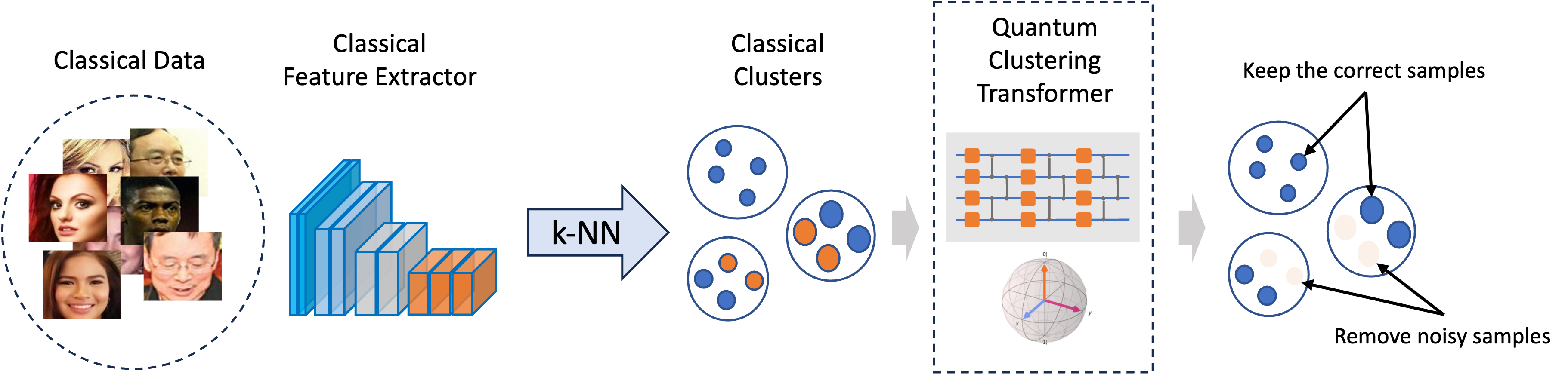
Inspired by the unique properties of Quantum machines, this paper presents an innovative Quantum clustering framework utilizing Transformer architecture to autonomously cluster samples in an unsupervised fashion. The approach demonstrates resilience in handling noisy and challenging samples, owing to its efficient self-attention mechanism. In addition, leveraging the benefits of Quantum computing, the method offers ease of optimization. The framework of the Quantum Transformer for Clustering is illustrated in Fig. 1.
The contributions of this work are threefold. Initially, we propose a Transformer-based method, named QClusformer, for visual clustering within the realm of Quantum Computing. Subsequently, we introduce a self-attention module and Transformer layers employing parameterized Quantum circuits. Lastly, the empirical experimental results on various benchmark datasets demonstrate the novelties and efficiency of our proposed approach compared to the corresponding classical machines.
In the remaining content of this paper, we provide some basic background for understanding this paper in Section III. Then, we introduce our motivation and approach to the Quantum Transformer framework in Section IV. We then present the implementation of Quantum Transformer for Clustering in Section V and experimental results in Section VI. Finally, we conclude our proposed QClusformer in Section VII.
II Related Work
II-A Unsupervised Clustering
Typically, these unsupervised clustering methods calculate the empirical density and identify clusters as dense areas within a data space, as seen in techniques like K-Means [16] and spectral clustering [19]. In addition, Otto et al. [20] proposed an approximate rank order metric for clustering millions of faces based on identity. Ankerst et al. [21] introduced a related concept focusing on ordering data points. Chen et al. [22] suggested an unsupervised hashing technique called Anchor-based Probability Hashing, aiming to maintain similarities by exploiting the data point distributions.
Face clustering tasks often encounter challenges with large-scale samples and intricate data distributions, drawing considerable research interest. Traditional unsupervised methods, hindered by their simplistic distribution assumptions like the convex shape assumption in K-Means [16] and the uniform density assumption in DBSCAN [18], tend to perform poorly. In recent years, supervised methods based on Graph Convolutional Networks (GCNs) have emerged as effective and efficient solutions for face clustering. L-GCN [23] employs GCNs for link prediction on subgraphs. Both DS-GCN [24] and VE-GCN [25] propose two-stage GCNs for clustering based on large k-nearest neighbor (kNN) graphs. DA-Net [26] conducts clustering by incorporating non-local context information through density-based graphs. Clusformer [27] utilizes a transformer architecture for face clustering. STAR-FC [28] introduces a structure-preserving sampling strategy to train the edge classification GCN. These advancements underscore the effectiveness of GCNs in representation learning and clustering.
II-B Quantum Unsupervised Clustering
There are several studies on the computer vision tasks, such as recognition and classification [29, 30], object tracking [31], transformation estimation [32], shape alignment and matching [33, 34, 35], permutation synchronization [36], and motion segmentation [37]. In light of this research, several studies [38, 39, 40, 41] have employed Quantum machines in unsupervised learning. Nonetheless, these methods replicate conventional classical techniques and encounter constraints when confronted with large databases like face or landmark clustering. Hence, developing a Quantum-based framework tailored for unsupervised clustering tasks with large-scale databases is imperative.
III Background
III-A Quantum Basics
A Quantum Bit or qubit is the information carrier in the Quantum computing and communication channel. A qubit is a two-dimensional Hilbert space with two orthonormal bases and . These computational bases are usually represented as vectors and . Due to the unique qubit characteristic of superposition, the state of a qubit can be represented as the sum of two computational bases weighted by (complex) amplitudes as follows,
| (1) |
where and , and . and are the probability of obtaining states and after multiple measurements, respectively. It gives an advantage in Quantum computing over classical computing when the qubits can be entangled. The two qubits and are entangled when they have a state that cannot be individually represented as a complex scalar times the basis vector. One example of an entangled qubits state is the Bell state represented as:
| (2) |
where is the tensor product of the basic vectors and in the state vector space of qubits and .
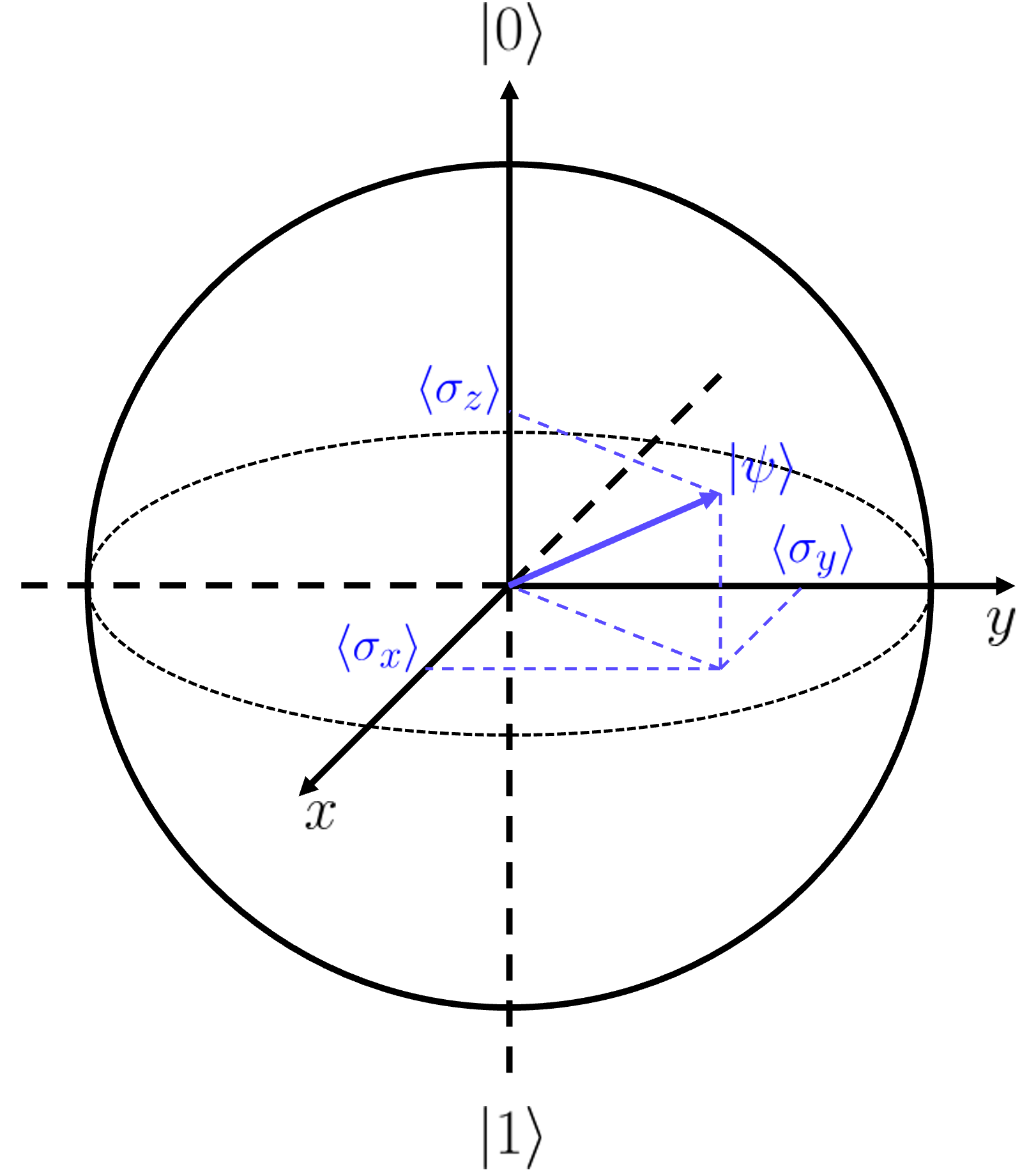
A Quantum state can be transformed to another state through a Quantum circuit represented by a unitary matrix . The Quantum state transformation can be mathematically formulated as . To get classical information from a Quantum state , Quantum measurements are applied by computing the expectation value of a Hermitian matrix . In most cases, the Pauli matrices, i.e., , , and , are used to measure the Quantum state as shown in Fig. 2. The Pauli matrices are defined as:
| (3) |
III-B Parameterized Quantum Circuit
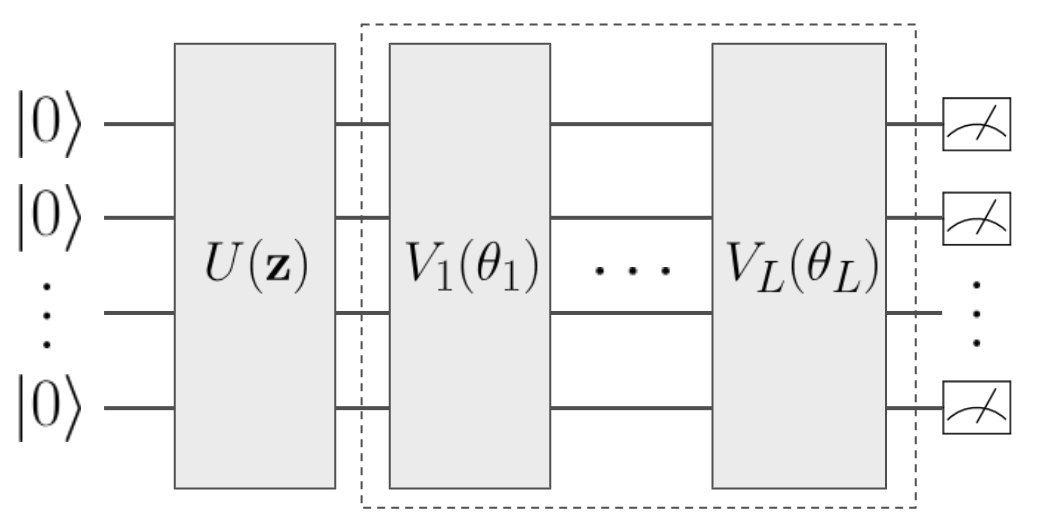
The parameterized Quantum circuit (PQC), also known as a variational Quantum circuit (VQC) [42], is a special kind of Quantum circuit with parameters that can be optimized or learned iteratively. The PQC comprises three parts: data encoding, parameterized layer, and Quantum measurements.
Given a classical data where is the data dimension, the data encoding circuit is used to transform into a Quantum state . The data encoding can be based on encoding methods such as basis, angle, or amplitude encoding. The Quantum state is transformed via the parameterized layer to a new state . The parameterized layer is a sequence of Quantum circuit operators with learnable parameters denoted as:
| (4) |
where is the number of operators. The learnable parameters can be updated via gradient-based [43], or gradient-free [44] algorithms. The Quantum measurements are used to retrieve the values of the Quantum state for further processing. Overall, the PQC can be formulated as:
| (5) |
where is a predefined observable.
PQC uses a hybrid Quantum-classical procedure to optimize the trainable parameters iteratively. The popular optimization approaches include gradient descent [45], parameter-shift rule [46, 43], and gradient-free techniques [47, 44]. All learning methods take the training data as input and evaluate the model performance by comparing the predicted and ground-truth labels. Based on this evaluation, the methods update the model parameters for the next iteration and repeat the process until the model converges and achieves the desired performance. The hybrid method performs the evaluation and parameter optimization on a classical computer, while the model inference is processed on a Quantum computer.
III-C Visual Clustering
Given a dataset where represents a data point in dimensional space, the objective of unsupervised clustering is to partition the dataset into clusters such that satisfies following conditions. Firstly, each data point belongs to exactly one cluster. Secondly, data points within the same cluster are more similar than those in different clusters. Depending on the predefined problem, the number of clusters can be determined automatically or specified beforehand. The goal is to find an optimal partitioning of the dataset that maximizes the intra-cluster similarity and minimizes the inter-cluster similarity. It is typically achieved by defining a suitable objective function or similarity measure and optimizing it to obtain cluster assignments. Formally, let represent the set of clusters, where denotes the cluster, and represents for the centroid (or center) of the . The task is to find an optimal partitioning that minimizes the following objective function, quantifying the dissimilarity between data points and their respective cluster centroids.
| (6) |
where denotes the distance between sample and centroid of the cluster . Common distance measures used in unsupervised clustering include Euclidean distance, Manhattan distance, cosine similarity, etc. The optimization process typically involves iterative procedures such as K-means, hierarchical clustering, density-based clustering, or spectral clustering to find the optimal partitioning that minimizes the objective function.
III-D Transformer
The Transformer [48] is a sequence-to-sequence model consisting of an encoder and a decoder. Each encoder and decoder is a stack of identical blocks. Each block is composed of a multi-head attention module and a feed-forward network. With the multi-head attention module, the Transformer can focus on different positions of an input sequence, leading to a robust deep network that outperforms prior methods.
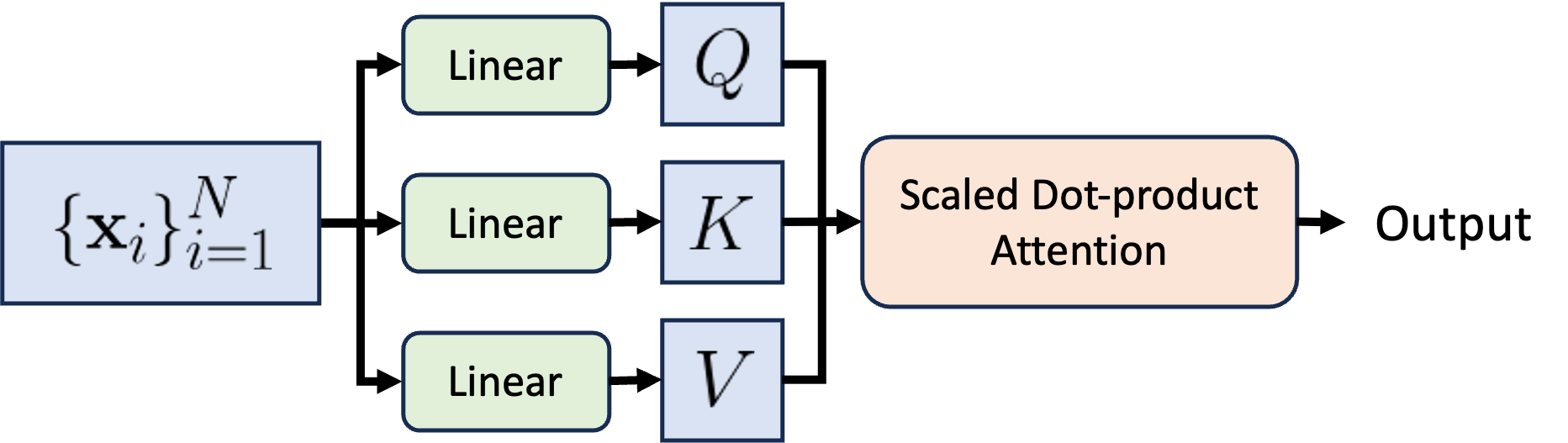
In each self-attention layer, the input data are linearly mapped via three weighted matrices, i.e., key , query , and value , to three parts , , and , respectively. The query and key parts are then applied to the inner product, and the output is computed as:
| (7) |
where
| (8) |
is the self-attention coefficient. Fig. 3 illustrates the framework of the self-attention module on classical data.
IV Our Proposed Approach
This section begins by outlining the motivations and underlying intuitions driving our paper. Following that, we delve into the process of encoding classical data, specifically feature representations, into the Quantum machine. Lastly, we detail the implementation of self-attention mechanisms and transformer blocks within the Quantum framework.
IV-A Motivations
Assume that we have employed a clustering algorithm, i.e., K-Nearest Neighbors (KNN), to form initial clusters . Given a cluster of samples with a center . This cluster may include erroneous samples due to various factors. Firstly, setting a fixed number of neighbors, denoted as , can result in clusters with fewer than samples, potentially containing noisy or inaccurate data points. Secondly, the lack of robustness in the feature extractor, such as a deep neural network, may cause the representations of distinct samples to be similar, resulting in samples from different subjects being differently grouped into the same cluster. Lastly, the unlabeled data may introduce challenging samples that closely resemble each other, causing misassignments in cluster allocation when employing K-NN.
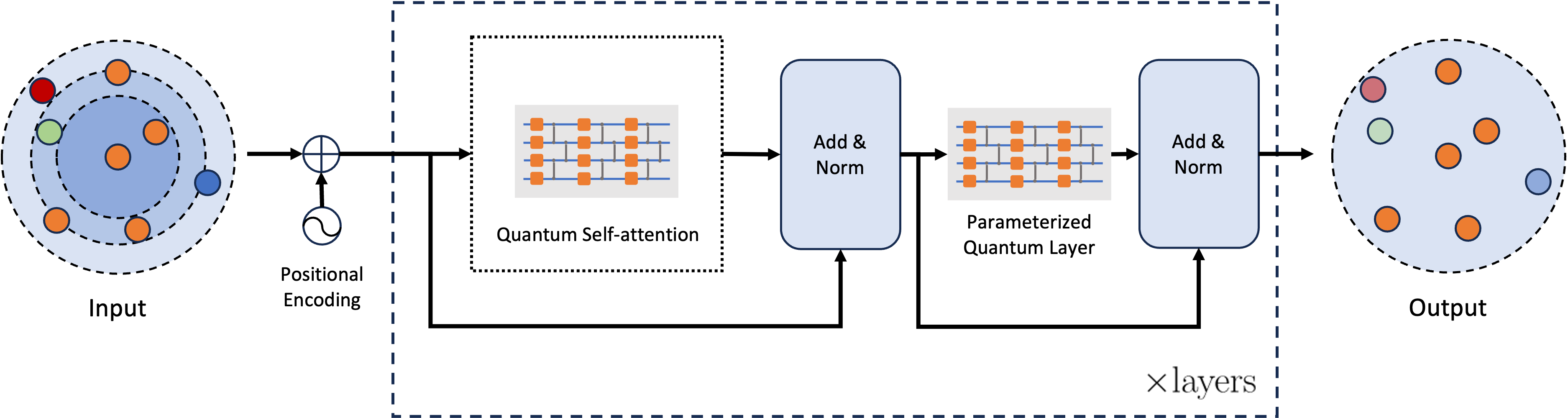
Numerous methodologies have tackled this problem on classical computers, employing a variety of techniques such as graph-based approaches [23, 25, 24, 28, 49, 50], and transformer-based methods [27]. Although transformer architectures have shown remarkable success in diverse computer vision tasks [51, 52, 53, 54, 55, 56, 57, 58, 59, 60, 61, 62, 63, 64, 65], their potential within Quantum computing remains promising. Hence, leveraging insights from classical Transformers, we expand its application to Quantum machines by conceptualizing the most important element of the Transformer, self-attention, through a Quantum perspective. With this concept, we construct successive Transformer blocks comprising self-attention modules and Variational Quantum Circuits (VQC) serving as linear layers to build a Quantum transformer architecture. We propose a Transformer-based clustering framework for Quantum machines to recognize the noisy or hard samples inside the cluster as in Fig. 4.
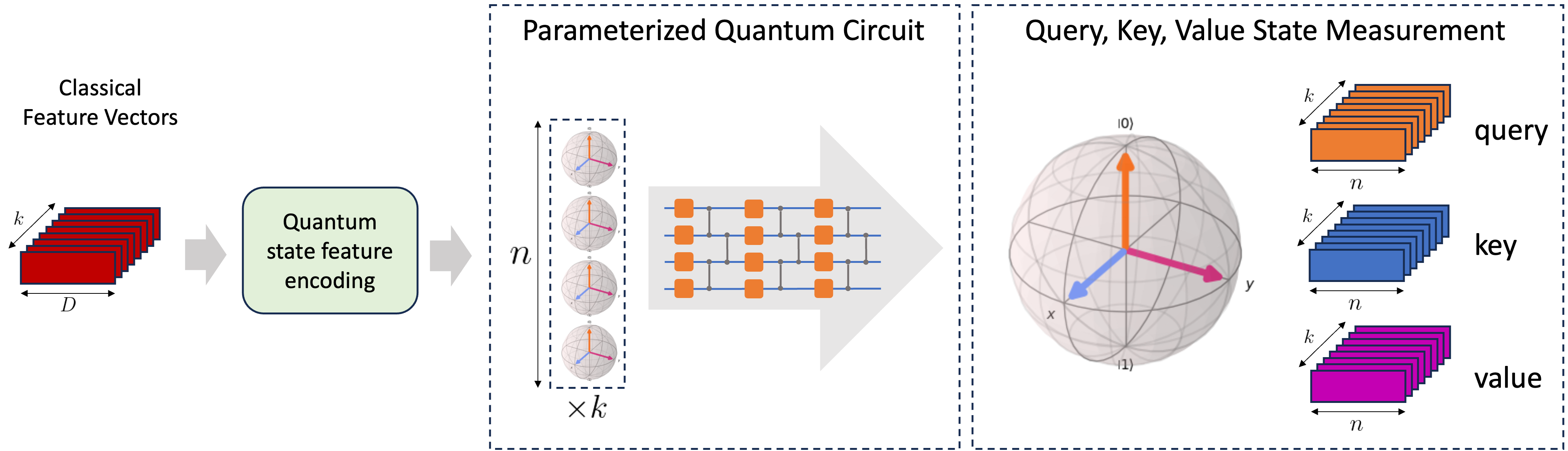
IV-B Quantum State Feature Encoding
To operate on a classical dataset for a Quantum circuit, it is important to define an encoding method to transform the classical feature vector into a Quantum state. As the number of qubits is limited, we need to encode the classical values with a small number of qubits as much as possible. Given qubits, a general Quantum state can be represented as
| (9) |
where is the amplitude of a Quantum state. The square of is the probability of measurement of the state in , and the sum of probabilities should be .
In this work, we use the amplitude encoding method to encode the classical vector into a Quantum state. Given a feature vector where , the Quantum state can be represented as
| (10) |
Indeed, to encode a -dimension feature vector, the minimum number of required qubits is . The encoded Quantum state can then be transformed by Quantum gates and then measured to a classical -dimension vector for the Quantum self-attention in a lower space dimension.
IV-C Quantum Transformer
In contrast to classical transformers, which employ linear transformations as detailed in Section III-D, PQCs transform classical features for self-attention. Given a sequential input , Quantum self-attention is introduced to compute the relationship between feature vectors in as follows:
| (11) |
In general, when provided with a -dimensional vector , our approach involves encoding the values into a Quantum state through an -qubit circuit. Following this, the Quantum state transforms a parameterized layer. Subsequently, the final state is measured for subsequent processing, typically utilizing the Pauli matrix as an observable in most applications. However, this design utilizes three parameterized Quantum circuits to compute the key, query, and value of the feature vectors, potentially not fully leveraging all the information encoded in the Quantum state.
Moreover, we found that given an arbitrary 1-qubit Quantum state , the density matrix can be expressed as a linear combination of Pauli matrices:
| (12) |
where and . The Pauli matrices have the following properties:
| (13) |
Then, for each observable , the expectation of the measurement is:
| (14) |
Eqn. 14 shows that the three Pauli matrices as observables measure three separated values of the Quantum state . Inspired by this property, we design a single parameterized Quantum circuit for the self-attention module as shown in Fig. 6. Each observable computes the key, query, or value of the feature vector. Given an -qubit parameterized Quantum circuit, the Quantum self-attention computes -dimension key, query, and value.
Let a QClusformer encoder be a stack of Quantum Transformer blocks where each block contains a Quantum self-attention (QSA) and a parameterized Quantum layer (PQL) :
| (15) |
where LN is the layer normalization. The procedures of QSA and PQL are described in Algorithm 1 and 2. The output of the QClusformer encoder is used for the clustering task.
V Implementation
V-A Visual Cluster Dataset
Given a set of features extracted from dataset , the k-nearest neighbors is applied to cluster the samples based on the cosine similarity score. They will be formed as a cluster having as the center:
| (16) |
where is the number of nearest neighbors. Then, we construct a clustered dataset denoted as . This dataset is used in the QClusformer, which will be described in the following sections.
V-B Cosine Similarity Encoding
As the Transformer processes the input represented as a sequence, the cluster has to be represented as a sequence for QClusformer. Generally, a Transformer encoder expects an input of a sequence similar to Recurrent Neural Networks or Long-Short Term Memory that is widely used in Natural Language Processing. As the Transformer processes words in parallel, a Positional Encoding is presented to preserve the order of the sequence. Unlike the sequence inputs, the cluster dataset follows the similarities between samples and the cluster centers. Thus, a Cosine Similarity Encoding is introduced to describe the structure of the cluster dataset. Let be the position of an element in the sequence input, be the Cosine Similarity Encoding as follows,
| (17) |
The feature of the -th element in the sequence turns to
| (18) |
where is a projected weight. The feature vector is then encoded into a Quantum state for the Quantum self-attention. The clustering dataset construction and encoding is shown as Algorithm 3.
V-C Objective and Loss Functions
Although the neighbors of center are expected to have the same label as the center, there are hard samples from various clusters in real-world conditions. Thus, cannot contain all visual samples in one label. The QClusformer is introduced to detect these hard samples. The output sequence is a binary sequence , where if the -th sample in the sequence has the same label as the center and vice versa. Let be the ground truth of the output, a Binary Cross Entropy loss is used to train the QClusformer:
| (19) |
V-D Implementation Details
We use ResNet50 [66] as a classical backbone to extract features from the images. We simulate the Quantum machine by utilizing the TorchQuantm library [67]. Since this library uses Pytorch as the backend, we can leverage GPUs and CUDA to speed up the training process. The models are trained utilizing an 8 A100 GPU setup, each with 40GB of memory. The learning rate is initially set to , progressively decreasing to zero following the CosineAnnealing policy [68]. Each GPU operates with a batch size of . The optimization uses AdamW [69] for epochs.
VI Experimental Results
VI-A Evaluation Metrics
To evaluate the performance of the methods, we use Fowlkes Mallows Score to measure the similarity between two clusters with a set of points. This score is computed by taking the geometry mean of precision and recall of the point pairs. Thus, Fowlkes Mallows Score is also called Pairwise F-score (), defined as:
| (20) |
where is the number of point pairs in the same cluster in both ground truth and prediction, is the number of point pairs in the same cluster in prediction but not in ground truth, and is the number of point pairs in the same cluster in ground truth but not prediction.
BCubed F-score is another popular metric for clustering evaluation focusing on each data point. For each data point , the BCubed computes the precision () and recall () as follows,
| (21) |
where is the number of points in the same cluster of point both in ground truth and prediction, is the number of points in the same cluster of point in prediction but not in ground truth, and is the number of points in the same cluster of point in ground truth but not prediction. Then, the BCubed F-score () is defined as:
| (22) |
where
| (23) |
| Method | Num. unlabeled | 584K | 1.74M | 2.89M | 4.05M | 5.21M | |||||
| QML | |||||||||||
| K-means [16, 17] | ✗ | 79.21 | 81.23 | 73.04 | 75.20 | 69.83 | 72.34 | 67.90 | 70.57 | 66.47 | 69.42 |
| HAC [70] | ✗ | 70.63 | 70.46 | 54.40 | 69.53 | 11.08 | 68.62 | 1.40 | 67.69 | 0.37 | 66.96 |
| DBSCAN [18] | ✗ | 67.93 | 67.17 | 63.41 | 66.53 | 52.50 | 66.26 | 45.24 | 44.87 | 44.94 | 44.74 |
| ARO [20] | ✗ | 13.60 | 17.00 | 8.78 | 12.42 | 7.30 | 10.96 | 6.86 | 10.50 | 6.35 | 10.01 |
| CDP [71] | ✗ | 75.02 | 78.70 | 70.75 | 75.82 | 69.51 | 74.58 | 68.62 | 73.62 | 68.06 | 72.92 |
| Classical Clusformer | ✗ | 63.31 | 79.74 | 60.23 | 78.14 | 58.53 | 76.84 | 56.79 | 75.92 | 55.13 | 75.01 |
| QClusformer | ✓ | 74.50 | 82.09 | 73.12 | 80.92 | 71.25 | 78.67 | 69.46 | 77.24 | 68.38 | 75.86 |
VI-B Datasets
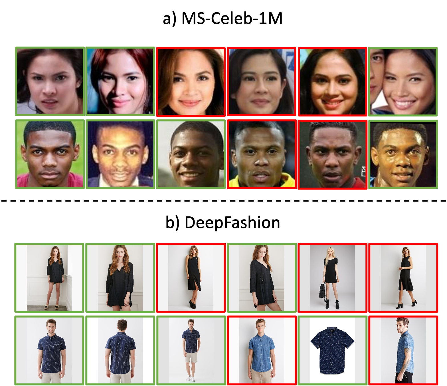
We follow [25] to use MS-Celeb-1M [72] and DeepFashion [73] datasets for experiments. The Fig. 7 illustrates samples of the datasets.
Face Clustering and Recognition. MS-Celeb-1M [72] is a large-scale face recognition dataset crawled from the Internet. The cleaned version consists of 85K identities with 5.8M images. The images are pre-processed by aligning and cropping to the size of . The MS-Celeb-1M dataset is randomly split into ten parts. Each part contains approximately 584K images of 8,500 identities. There is no identity overlapped among them.
Clothes Clustering. DeepFashion [73] is a large-scale clothes recognition dataset. Inspired by Yang et al. [25] for clustering, the DeepFashion dataset is split into 25,752 images of 3,997 categories for training and 26,960 images of 3,984 categories for testing. Similar to the face clustering setting, no overlapped category exists between the training and testing sets.
VI-C Performance on MS-Celeb-1M Clustering
Table I illustrates the performance of our proposed method on the MS-Celeb-1M Clustering benchmark. Following the benchmarks from the previous studies [27, 74, 23, 24, 25], we first train the classical feature extractor on the first part of the MS-Celeb-1M dataset in a supervised manner. Then, we construct the cluster dataset using -nearest neighbor and train the QClusformer model. The trained QClusformer model is evaluated on five accumulated parts as shown in Table I. Due to hardware constraints, we can only simulate the QClusformer with the number of Transformer blocks . For a fair comparison, we train the classical Clustering Transformer with the same number of blocks. Compared to the classical Clustering Transformer, the proposed QClusformer achieves higher performance with a Pairwise F1-score from to and BCubed F1-score from to on the 584K testing part. Similar performance trends are shown across all testing parts of MS-Celeb-1M.
VI-D Performance on DeepFashion Clustering
| Method | QML | ||
| K-means [16, 17] | ✗ | 32.86 | 53.77 |
| HAC [70] | ✗ | 22.54 | 48.77 |
| DBSCAN [18] | ✗ | 25.07 | 53.23 |
| Mean shift [75] | ✗ | 31.61 | 56.73 |
| Spectral [19] | ✗ | 29.02 | 46.40 |
| Classical Clusformer | ✗ | 35.62 | 60.61 |
| QClusformer | ✓ | 35.71 | 60.00 |
We compare the performance of our proposed method on the DeepFashion dataset for the clustering task as shown in Table II. The evaluation protocols on the DeepFashion clustering task are the same as the MS-Celeb-1M clustering benchmark. While achieving higher performance than the previous classical clustering methods with a Pairwise F1-score of and BCubed F1-score of , the proposed QClusformer method maintains competitive results compared to the classical Transformer setting.
VI-E Ablation Studies
| 100 classes | Pair-wise | BCubed | ||||
| Precision | Recall | F1-score | Precision | Recall | F1-score | |
| QKMeans [76] | 88.06 | 81.02 | 84.40 | 89.84 | 88.00 | 88.91 |
| QClusformer | 90.37 | 80.88 | 85.36 | 93.99 | 88.47 | 91.15 |
| 1000 classes | Pair-wise | BCubed | ||||
| Precision | Recall | F1-score | Precision | Recall | F1-score | |
| QKMeans [76] | 73.35 | 36.61 | 48.84 | 75.91 | 68.38 | 71.95 |
| QClusformer | 68.16 | 45.68 | 54.70 | 79.84 | 70.59 | 74.93 |
Comparison with previous Quantum Clustering method. Table III compares the proposed and prior clustering methods on Quantum computing, i.e., QKMeans [76]. We evaluate the methods on subsets of the DeepFashion dataset with 100 categories and 1000 categories. In the 100-class setting, compared to prior work, the proposed method improves the Pairwise and BCubed F1-score from to and from to respectively. The same results trend is shown in the 1000-class setting with higher margins.
| QML | Transformer Circuits | Pair-wise | BCubed | ||||
| Precision | Recall | F1-score | Precision | Recall | F1-score | ||
| - | 57.35 | 25.83 | 35.62 | 79.73 | 48.89 | 60.61 | |
| ✓ | 1Q-1K-1V | 41.97 | 31.08 | 35.71 | 65.57 | 55.30 | 60.00 |
| ✓ | 1QK-1V | 42.79 | 29.70 | 35.06 | 66.98 | 54.31 | 59.98 |
| ✓ | 1QKV | 43.09 | 29.67 | 35.14 | 67.55 | 54.12 | 60.10 |
Comparison with different QClusformer settings. Table IV shows the experimental results in different settings of the proposed QClusformer method on the DeepFashion dataset [73]. We use three different PQC settings of Quantum self-attention, i.e., three PQCs each for query, key, and value (1Q-1K-1V); one PQC for query and key and one PQC for value (1QK-1V); and one PQC for query, key, and value (1QKV). Compared to the classical clustering transformer setting, the proposed QClusformer settings competitive results with the best Pairwise F1-score of with the 1Q-1K-1V setting and the best BCubed F1-score of with the 1QKV setting. The 1QKV setting uses one PQC for Quantum self-attention with competitive results, which shows the ability to utilize the information of the Quantum state.
VII Conclusion
In this paper, we have proposed QClusformer, a Quantum approach, for Transformer-based vision clustering problems. The QClusformer method utilizes Parameterized Quantum Circuits to leverage the Quantum information in self-attention computing. By separating the values of a Quantum state via Pauli matrices for measurement, we minimize the usage of Quantum computing resources for the self-attention module. The competitive evaluation results on multiple large-scale vision clustering benchmarks have demonstrated the potential of the proposed Transformer-base clustering framework on Quantum computing in various applications.
References
- [1] J. Preskill, “Quantum computing and the entanglement frontier,” arXiv preprint arXiv:1203.5813, 2012.
- [2] ——, “Quantum computing in the nisq era and beyond,” Quantum, vol. 2, p. 79, 2018.
- [3] S. Boixo, S. V. Isakov, V. N. Smelyanskiy, R. Babbush, N. Ding, Z. Jiang, M. J. Bremner, J. M. Martinis, and H. Neven, “Characterizing quantum supremacy in near-term devices,” Nature Physics, vol. 14, no. 6, pp. 595–600, 2018.
- [4] A. Basheer, A. Afham, and S. K. Goyal, “Quantum -nearest neighbors algorithm,” arXiv preprint arXiv:2003.09187, 2020.
- [5] P. Rebentrost, M. Mohseni, and S. Lloyd, “Quantum support vector machine for big data classification,” Physical review letters, vol. 113, no. 13, p. 130503, 2014.
- [6] D. Horn and A. Gottlieb, “The method of quantum clustering,” Advances in neural information processing systems, vol. 14, 2001.
- [7] ——, “Algorithm for data clustering in pattern recognition problems based on quantum mechanics,” Physical review letters, vol. 88, no. 1, p. 018702, 2001.
- [8] X. B. Nguyen, B. Thompson, H. Churchill, K. Luu, and S. U. Khan, “Quantum vision clustering,” arXiv preprint arXiv:2309.09907, 2023.
- [9] A. A. Ezhov and D. Ventura, “Quantum neural networks,” Future Directions for Intelligent Systems and Information Sciences: The Future of Speech and Image Technologies, Brain Computers, WWW, and Bioinformatics, pp. 213–235, 2000.
- [10] M.-G. Zhou, Z.-P. Liu, H.-L. Yin, C.-L. Li, T.-K. Xu, and Z.-B. Chen, “Quantum neural network for quantum neural computing,” Research, vol. 6, p. 0134, 2023.
- [11] B. Gupta and S. Dhawan, “Quantum neural network (qnn) research a scientometrics assessment of global publications during 1990-2019.” International Journal of Information Dissemination & Technology, vol. 10, no. 3, 2020.
- [12] A. Dendukuri, B. Keeling, A. Fereidouni, J. Burbridge, K. Luu, and H. Churchill, “Defining quantum neural networks via quantum time evolution,” Quantum Machine Learning Conference, 2019.
- [13] A. Dendukuri and K. Luu, “Image processing in quantum computers,” Quantum Machine Learning Conference, 2019.
- [14] J. Biamonte, P. Wittek, N. Pancotti, P. Rebentrost, N. Wiebe, and S. Lloyd, “Quantum machine learning,” Nature, vol. 549, no. 7671, pp. 195–202, 2017.
- [15] Y. Du, M.-H. Hsieh, T. Liu, and D. Tao, “Expressive power of parametrized quantum circuits,” Physical Review Research, vol. 2, no. 3, p. 033125, 2020.
- [16] S. Lloyd, “Least squares quantization in pcm,” IEEE transactions on information theory, vol. 28, no. 2, pp. 129–137, 1982.
- [17] D. Sculley, “Web-scale k-means clustering,” in Proceedings of the 19th international conference on World wide web, 2010, pp. 1177–1178.
- [18] M. Ester, H.-P. Kriegel, J. Sander, X. Xu et al., “A density-based algorithm for discovering clusters in large spatial databases with noise,” in kdd, vol. 96, no. 34, 1996, pp. 226–231.
- [19] A. Ng, M. Jordan, and Y. Weiss, “On spectral clustering: Analysis and an algorithm,” Advances in neural information processing systems, vol. 14, 2001.
- [20] C. Otto, D. Wang, and A. K. Jain, “Clustering millions of faces by identity,” IEEE transactions on pattern analysis and machine intelligence, vol. 40, no. 2, pp. 289–303, 2017.
- [21] M. Ankerst, M. M. Breunig, H.-P. Kriegel, and J. Sander, “Optics: Ordering points to identify the clustering structure,” ACM Sigmod record, vol. 28, no. 2, pp. 49–60, 1999.
- [22] J. Chen, W. K. Cheung, and A. Wang, “Aphash: Anchor-based probability hashing for image retrieval,” in 2018 IEEE International Conference on Acoustics, Speech and Signal Processing (ICASSP). IEEE, 2018, pp. 1673–1677.
- [23] Z. Wang, L. Zheng, Y. Li, and S. Wang, “Linkage based face clustering via graph convolution network,” in Proceedings of the IEEE/CVF conference on computer vision and pattern recognition, 2019, pp. 1117–1125.
- [24] L. Yang, X. Zhan, D. Chen, J. Yan, C. C. Loy, and D. Lin, “Learning to cluster faces on an affinity graph,” in Proceedings of the IEEE/CVF conference on computer vision and pattern recognition, 2019, pp. 2298–2306.
- [25] L. Yang, D. Chen, X. Zhan, R. Zhao, C. C. Loy, and D. Lin, “Learning to cluster faces via confidence and connectivity estimation,” in Proceedings of the IEEE/CVF conference on computer vision and pattern recognition, 2020, pp. 13 369–13 378.
- [26] S. Guo, J. Xu, D. Chen, C. Zhang, X. Wang, and R. Zhao, “Density-aware feature embedding for face clustering,” in Proceedings of the IEEE/CVF Conference on Computer Vision and Pattern Recognition, 2020, pp. 6698–6706.
- [27] X.-B. Nguyen, D. T. Bui, C. N. Duong, T. D. Bui, and K. Luu, “Clusformer: A transformer based clustering approach to unsupervised large-scale face and visual landmark recognition,” in Proceedings of the IEEE/CVF conference on computer vision and pattern recognition, 2021, pp. 10 847–10 856.
- [28] S. Shen, W. Li, Z. Zhu, G. Huang, D. Du, J. Lu, and J. Zhou, “Structure-aware face clustering on a large-scale graph with 107 nodes,” in Proceedings of the IEEE/CVF Conference on Computer Vision and Pattern Recognition, 2021, pp. 9085–9094.
- [29] D. O’Malley, V. V. Vesselinov, B. S. Alexandrov, and L. B. Alexandrov, “Nonnegative/binary matrix factorization with a d-wave quantum annealer,” PloS one, vol. 13, no. 12, p. e0206653, 2018.
- [30] G. Cavallaro, D. Willsch, M. Willsch, K. Michielsen, and M. Riedel, “Approaching remote sensing image classification with ensembles of support vector machines on the d-wave quantum annealer,” in IGARSS 2020-2020 IEEE International Geoscience and Remote Sensing Symposium. IEEE, 2020, pp. 1973–1976.
- [31] J. Li and S. Ghosh, “Quantum-soft qubo suppression for accurate object detection,” in European Conference on Computer Vision. Springer, 2020, pp. 158–173.
- [32] V. Golyanik and C. Theobalt, “A quantum computational approach to correspondence problems on point sets,” in Proceedings of the IEEE/CVF Conference on Computer Vision and Pattern Recognition, 2020, pp. 9182–9191.
- [33] M. Noormandipour and H. Wang, “Matching point sets with quantum circuit learning,” in ICASSP 2022-2022 IEEE International Conference on Acoustics, Speech and Signal Processing (ICASSP). IEEE, 2022, pp. 8607–8611.
- [34] M. S. Benkner, Z. Lähner, V. Golyanik, C. Wunderlich, C. Theobalt, and M. Moeller, “Q-match: Iterative shape matching via quantum annealing,” in Proceedings of the IEEE/CVF International Conference on Computer Vision, 2021, pp. 7586–7596.
- [35] M. S. Benkner, V. Golyanik, C. Theobalt, and M. Moeller, “Adiabatic quantum graph matching with permutation matrix constraints,” in 2020 International Conference on 3D Vision (3DV). IEEE, 2020, pp. 583–592.
- [36] T. Birdal, V. Golyanik, C. Theobalt, and L. J. Guibas, “Quantum permutation synchronization,” in Proceedings of the IEEE/CVF Conference on Computer Vision and Pattern Recognition, 2021, pp. 13 122–13 133.
- [37] F. Arrigoni, W. Menapace, M. S. Benkner, E. Ricci, and V. Golyanik, “Quantum motion segmentation,” in European Conference on Computer Vision. Springer, 2022, pp. 506–523.
- [38] C. Dürr, M. Heiligman, P. HOyer, and M. Mhalla, “Quantum query complexity of some graph problems,” SIAM Journal on Computing, vol. 35, no. 6, pp. 1310–1328, 2006.
- [39] Q. Li, Y. He, and J.-p. Jiang, “A novel clustering algorithm based on quantum games,” Journal of Physics A: Mathematical and Theoretical, vol. 42, no. 44, p. 445303, 2009.
- [40] ——, “A hybrid classical-quantum clustering algorithm based on quantum walks,” Quantum Information Processing, vol. 10, pp. 13–26, 2011.
- [41] Y. Yu, F. Qian, and H. Liu, “Quantum clustering-based weighted linear programming support vector regression for multivariable nonlinear problem,” Soft Computing, vol. 14, pp. 921–929, 2010.
- [42] M. Benedetti, E. Lloyd, S. Sack, and M. Fiorentini, “Parameterized quantum circuits as machine learning models,” Quantum Science and Technology, vol. 4, no. 4, p. 043001, 2019.
- [43] K. Mitarai, M. Negoro, M. Kitagawa, and K. Fujii, “Quantum circuit learning,” Physical Review A, vol. 98, no. 3, p. 032309, 2018.
- [44] S. Y.-C. Chen, C.-M. Huang, C.-W. Hsing, H.-S. Goan, and Y.-J. Kao, “Variational quantum reinforcement learning via evolutionary optimization,” Machine Learning: Science and Technology, vol. 3, no. 1, p. 015025, 2022.
- [45] R. Sweke, F. Wilde, J. Meyer, M. Schuld, P. K. Fährmann, B. Meynard-Piganeau, and J. Eisert, “Stochastic gradient descent for hybrid quantum-classical optimization,” Quantum, vol. 4, p. 314, 2020.
- [46] D. Wierichs, J. Izaac, C. Wang, and C. Y.-Y. Lin, “General parameter-shift rules for quantum gradients,” Quantum, vol. 6, p. 677, 2022.
- [47] G. Nannicini, “Performance of hybrid quantum-classical variational heuristics for combinatorial optimization,” Physical Review E, vol. 99, no. 1, p. 013304, 2019.
- [48] A. Vaswani, N. Shazeer, N. Parmar, J. Uszkoreit, L. Jones, A. N. Gomez, Ł. Kaiser, and I. Polosukhin, “Attention is all you need,” Advances in neural information processing systems, vol. 30, 2017.
- [49] S. Shen, W. Li, X. Wang, D. Zhang, Z. Jin, J. Zhou, and J. Lu, “Clip-cluster: Clip-guided attribute hallucination for face clustering,” in Proceedings of the IEEE/CVF International Conference on Computer Vision, 2023, pp. 20 786–20 795.
- [50] J. Shin, H.-J. Lee, H. Kim, J.-H. Baek, D. Kim, and Y. J. Koh, “Local connectivity-based density estimation for face clustering,” in Proceedings of the IEEE/CVF Conference on Computer Vision and Pattern Recognition, 2023, pp. 13 621–13 629.
- [51] J. Li, D. Li, C. Xiong, and S. Hoi, “Blip: Bootstrapping language-image pre-training for unified vision-language understanding and generation,” in International Conference on Machine Learning. PMLR, 2022, pp. 12 888–12 900.
- [52] J. Yu, Z. Wang, V. Vasudevan, L. Yeung, M. Seyedhosseini, and Y. Wu, “Coca: Contrastive captioners are image-text foundation models,” arXiv preprint arXiv:2205.01917, 2022.
- [53] X. Zhai, B. Mustafa, A. Kolesnikov, and L. Beyer, “Sigmoid loss for language image pre-training,” arXiv preprint arXiv:2303.15343, 2023.
- [54] Z. Luo, P. Zhao, C. Xu, X. Geng, T. Shen, C. Tao, J. Ma, Q. Lin, and D. Jiang, “Lexlip: Lexicon-bottlenecked language-image pre-training for large-scale image-text sparse retrieval,” in Proceedings of the IEEE/CVF International Conference on Computer Vision, 2023, pp. 11 206–11 217.
- [55] T. Wang, K. Lin, L. Li, C.-C. Lin, Z. Yang, H. Zhang, Z. Liu, and L. Wang, “Equivariant similarity for vision-language foundation models,” arXiv preprint arXiv:2303.14465, 2023.
- [56] X.-B. Nguyen, C. N. Duong, X. Li, S. Gauch, H.-S. Seo, and K. Luu, “Micron-bert: Bert-based facial micro-expression recognition,” in Proceedings of the IEEE/CVF Conference on Computer Vision and Pattern Recognition, 2023, pp. 1482–1492.
- [57] H.-Q. Nguyen, T.-D. Truong, X. B. Nguyen, A. Dowling, X. Li, and K. Luu, “Insect-foundation: A foundation model and large-scale 1m dataset for visual insect understanding,” arXiv preprint arXiv:2311.15206, 2023.
- [58] X.-B. Nguyen, G. S. Lee, S. H. Kim, and H. J. Yang, “Self-supervised learning based on spatial awareness for medical image analysis,” IEEE Access, vol. 8, pp. 162 973–162 981, 2020.
- [59] X.-B. Nguyen, G.-S. Lee, S.-H. Kim, and H.-J. Yang, “Audio-video based emotion recognition using minimum cost flow algorithm,” in 2019 IEEE/CVF International Conference on Computer Vision Workshop (ICCVW). IEEE, 2019, pp. 3737–3741.
- [60] B. Nguyen-Xuan and G.-S. Lee, “Sketch recognition using lstm with attention mechanism and minimum cost flow algorithm,” International Journal of Contents, vol. 15, no. 4, pp. 8–15, 2019.
- [61] P. Nguyen, K. G. Quach, C. N. Duong, N. Le, X.-B. Nguyen, and K. Luu, “Multi-camera multiple 3d object tracking on the move for autonomous vehicles,” in Proceedings of the IEEE/CVF Conference on Computer Vision and Pattern Recognition, 2022, pp. 2569–2578.
- [62] X. B. Nguyen, A. Bisht, H. Churchill, and K. Luu, “Two-dimensional quantum material identification via self-attention and soft-labeling in deep learning,” arXiv preprint arXiv:2205.15948, 2022.
- [63] X.-B. Nguyen, X. Liu, X. Li, and K. Luu, “The algonauts project 2023 challenge: Uark-ualbany team solution,” arXiv preprint arXiv:2308.00262, 2023.
- [64] X.-B. Nguyen, X. Li, S. U. Khan, and K. Luu, “Brainformer: Modeling mri brain functions to machine vision,” arXiv preprint arXiv:2312.00236, 2023.
- [65] X.-B. Nguyen, C. N. Duong, M. Savvides, K. Roy, and K. Luu, “Fairness in visual clustering: A novel transformer clustering approach,” arXiv preprint arXiv:2304.07408, 2023.
- [66] K. He, X. Zhang, S. Ren, and J. Sun, “Deep residual learning for image recognition,” in Proceedings of the IEEE conference on computer vision and pattern recognition, 2016, pp. 770–778.
- [67] H. Wang, Y. Ding, J. Gu, Z. Li, Y. Lin, D. Z. Pan, F. T. Chong, and S. Han, “Quantumnas: Noise-adaptive search for robust quantum circuits,” in The 28th IEEE International Symposium on High-Performance Computer Architecture (HPCA-28), 2022.
- [68] I. Loshchilov and F. Hutter, “Sgdr: Stochastic gradient descent with warm restarts,” arXiv preprint arXiv:1608.03983, 2016.
- [69] ——, “Decoupled weight decay regularization,” arXiv preprint arXiv:1711.05101, 2017.
- [70] R. Sibson, “Slink: an optimally efficient algorithm for the single-link cluster method,” The computer journal, vol. 16, no. 1, pp. 30–34, 1973.
- [71] X. Zhan, Z. Liu, J. Yan, D. Lin, and C. C. Loy, “Consensus-driven propagation in massive unlabeled data for face recognition,” in Proceedings of the European conference on computer vision (ECCV), 2018, pp. 568–583.
- [72] Y. Guo, L. Zhang, Y. Hu, X. He, and J. Gao, “Ms-celeb-1m: A dataset and benchmark for large-scale face recognition,” in Computer Vision–ECCV 2016: 14th European Conference, Amsterdam, The Netherlands, October 11-14, 2016, Proceedings, Part III 14. Springer, 2016, pp. 87–102.
- [73] Z. Liu, P. Luo, S. Qiu, X. Wang, and X. Tang, “Deepfashion: Powering robust clothes recognition and retrieval with rich annotations,” in Proceedings of the IEEE conference on computer vision and pattern recognition, 2016, pp. 1096–1104.
- [74] Y. Wang, Y. Zhang, F. Zhang, M. Lin, Y. Zhang, S. Wang, and X. Sun, “Ada-nets: Face clustering via adaptive neighbour discovery in the structure space,” arXiv preprint arXiv:2202.03800, 2022.
- [75] D. Comaniciu and P. Meer, “Mean shift: A robust approach toward feature space analysis,” IEEE Transactions on pattern analysis and machine intelligence, vol. 24, no. 5, pp. 603–619, 2002.
- [76] D. Quiroga, P. Date, and R. Pooser, “Discriminating quantum states with quantum machine learning,” in 2021 International Conference on Rebooting Computing (ICRC). IEEE, 2021, pp. 56–63.