Summing divergent matrix series

Abstract.

We extend several celebrated methods in classical analysis for summing series of complex numbers to series of complex matrices. These include the summation methods of Abel, Borel, Cesáro, Euler, Lambert, Nörlund, and Mittag-Leffler, which are frequently used to sum scalar series that are divergent in the conventional sense. One feature of our matrix extensions is that they are fully noncommutative generalizations of their scalar counterparts — not only is the scalar series replaced by a matrix series, positive weights are replaced by positive definite matrix weights, order on $\mathbb{R}$ replaced by Loewner order, exponential function replaced by matrix exponential function, etc. We will establish the regularity of our matrix summation methods, i.e., when applied to a matrix series convergent in the conventional sense, we obtain the same value for the sum. Our second goal is to provide numerical algorithms that work in conjunction with these summation methods. We discuss how the block and mixed-block summation algorithms, the Kahan compensated summation algorithm, may be applied to matrix sums with similar roundoff error bounds. These summation methods and algorithms apply not only to power or Taylor series of matrices but to any general matrix series including matrix Fourier and Dirichlet series. We will demonstrate the utility of these summation methods: establishing a Fejér’s theorem and alleviating the Gibbs phenomenon for matrix Fourier series; extending the domains of matrix functions and accurately evaluating them; enhancing the matrix Padé approximation and Schur–Parlett algorithms; and more.

1. Introduction

As we learned in calculus or real analysis, whenever we have an expression

$$\sum_{k=0}^{\infty}a_{k}=s$$ (1.1)

for some $a_{k}\in\mathbb{C}$, $k=0,1,2,\dots$, and $s\in\mathbb{C}$, the meaning of ‘$=$’ is defined to be the convergence of the sequence of partial sums $s_{n}\coloneqq\sum_{k=0}^{n}a_{k}$ to the limit $s$ in the standard Euclidean metric $\lvert\,\cdot\,\rvert$ on $\mathbb{C}$. In this case the series $\sum_{k=0}^{\infty}a_{k}$ is said to be convergent with value $s$; and if it does not meet this definition of convergence, then it is said to be divergent.

Because of its ubiquity and utility, we sometimes lose sight of the fact that such an interpretation of ‘$=$’ in (1.1) is purely by convention, and not sacrosanct. A series divergent in the sense of the conventional definition may have a well-defined value under alternative definitions of ‘$=$’ that are perfectly legitimate mathematically. Take the harmonic series $\sum_{k=1}^{\infty}1/k$ for illustration, well-known to be divergent in the conventional sense but as soon as we change, say, the choice of the metric from Euclidean to $p$-adic $\lvert\,\cdot\,\rvert_{p}$, it becomes convergent in the sense that $\lvert s_{n}-s\rvert_{p}\to 0$ for some value $s\in\mathbb{C}$ that depends on $p$ [8]. Indeed, a well-known result in $p$-adic analysis [40] is that with a $p$-adic metric, a series $\sum_{k=0}^{\infty}a_{k}$ is convergent if and only if $\lim_{k\to\infty}a_{k}=0$, obviously false by the conventional definition of series convergence.

Even if we restrict ourselves to the Euclidean metric, which is what we will do in the rest of this article, the meaning of ‘$=$’ still depends on a specific way to sum the values $a_{k}\in\mathbb{C}$, $k=0,1,2,\dots$. As is known to early analysts, there are many other reasonable ways to assign a value to a series that is divergent in the conventional sense, and such values are mathematically informative and useful in many ways [20]. As Hardy pointed out [20], a summation method just needs to be a function from the set of infinite series to values, assigning a sum to a series, which may or may not be convergent in the conventional sense.

The first and best-known summation method is likely Cesáro summation [10], that allows one to sum the Grandi series $1-1+1-1+\dotsb$ to $1/2$. The idea can be traced back even earlier to Leibniz, d’Alambert, Cauchy, and other predecessors of Cesáro [20, 44]. Cesáro summation has the property of being regular, i.e., for a series that is convergent in the conventional sense, the method gives an identical value for the sum. Regular summation methods have been studied extensively [4, 20, 38, 44] and applied in various fields from analytic number theory [46] to quantum field theory [15] to statistics [18]. Indeed summing divergent series is an important aspect of renormalization, a cornerstone of modern physics [45], particularly in the renormalization technique of zeta function regularization [22].

A main goal of our article is to show that many if not most of these summation methods for series of complex numbers extend readily and naturally to series of complex matrices. Take a toy example for illustration: The Neumann series

$$\sum_{k=0}^{\infty}X^{k}=(I-X)^{-1}$$ (1.2)

if and only if the spectral radius of $X\in\mathbb{C}^{d\times d}$ is less than $1$. Again ‘$=$’ here is interpreted in the sense of conventional summation, i.e., the sequence of partial sums $S_{n}\coloneqq\sum_{k=0}^{n}X^{k}$ converges to $(I-X)^{-1}$ with respect to any matrix norm $\lVert\,\cdot\,\rVert$. Let $\lambda(X)$ denote the spectrum of $X$ and $\mathbb{D}\coloneqq\{z\in\mathbb{C}:\lvert z\rvert<1\}$ the complex open unit disc. Depending on which method we use to sum the series on the left-hand side of (1.2), we obtain different interpretations of ‘$=$’:

conventional:

(1.2) holds if and only if $\lambda(X)\subseteq\mathbb{D}$;

Abel:

(1.2) holds if and only if $\lambda(X)\subseteq\overline{\mathbb{D}}\setminus\{1\}$;

Cesáro:

(1.2) holds if and only if $\lambda(X)\subseteq\mathbb{D}$ or $\lambda(X)\subseteq\overline{\mathbb{D}}\setminus\{1\}$ and the geometric and algebraic multiplicities are equal for each eigenvalue in $\lambda(X)\cap\partial\mathbb{D}\setminus\{1\}$;

Euler:

(1.2) holds if and only if $\lambda((I+P)^{-1}(P+X))\subseteq\mathbb{D}$ for some $P\succ 0$ commuting with $X$;

Borel:

(1.2) holds if and only if $\lambda(X)\subseteq\{z\in\mathbb{C}:\operatorname{Re}(\lambda)<1\}$.

The last four summation methods will be defined in due course. In case the reader is wondering, although the matrix $(I-X)^{-1}$ is well-defined as long as $1\notin\lambda(X)$, we will see that there is no natural method that will extend the validity of (1.2) to all $X\in\mathbb{C}^{d\times d}$ with $\lambda(X)\subseteq\mathbb{C}\setminus\{1\}$.

In the toy example above, the series in question is a power series where the $k$th term is a scalar multiple of $X^{k}$. The matrix summation methods in our article will apply more generally to any series of matrices $\sum_{k=0}^{\infty}A_{k}$, where $A_{k}$ may not be Taylor in nature, i.e., $(X-\alpha I)^{k}$, but may be Fourier $\sin(kX)$, Dirichlet $\exp(X\log k)$, Hadamard powers $X^{\circ k}$, or yet other forms not covered in this article, e.g., it could be defined by a recurrence relation $A_{k}=BA_{k-1}(I-A_{k-1})$ or randomly generated $A_{k}\sim\operatorname{\textsc{Wishart}}(\Sigma,n)$.

So a second goal of our article is to provide practical numerical algorithms that complement our theoretical summation methods. These algorithms will allow us to compute, in standard floating point arithmetic, a matrix $\widehat{S}\in\mathbb{C}^{d\times d}$ that approximates the theoretical sum $S\in\mathbb{C}^{d\times d}$ of the series $\sum_{k=0}^{\infty}A_{k}$ given by the respective summation method.

These two aspects are complementary: There is no numerical method that would allow one to ascertain the convergence of a series, regardless of which summation method we use. A standard example is the harmonic series $\sum_{k=1}^{\infty}1/k$; every numerical method would yield a finite value [23, Section 4.2], which is completely meaningless since its true value is $+\infty$. On the other hand, most of the matrix series we encounter will have no alternate closed-form expressions, again regardless of which summation method we use. The only way to obtain an approximate value would be through computing one in floating point arithmetic. In summary, the theoretical summation method permits us to determine convergence; and its corresponding numerical algorithm permits us to determine an approximate value. We provide an overview of these two aspects of our work.

Theoretical: regular summation methods

As in the case of its scalar counterpart, a matrix summation method is a partial function, i.e., possibly defined on a subset of its stated domain, from the set of $d\times d$ complex matrix series to a sum in $\mathbb{C}^{d\times d}$. We will generalize five classes of summation methods for scalar-valued series to matrix-valued ones. Figure 1 organizes them in a tree.

Figure 1. Relations between various methods: $a\to b$ means $a$-summation is a special case of $b$-summation; $a\twoheadrightarrow b$ means $a$-summable implies $b$-summable.

The five summation methods fall under two broad categories, sequential and functional methods, discussed in Sections 3 and 4 respectively. These terminologies follow those for scalar-valued series [44]. Basically, a sequential method transforms the terms of a series or its sequence of partial sums into another sequence, whereas a functional method would transform them into a function. We will generalize two of the most important sequential methods, Nörlund (of which Cesáro is a special case) and Euler; and three of the most important functional methods, Lambert, Abelian means, and Mittag-Leffler (Abel and Borel summations are respectively special cases of the latter two); showing that they also work for matrix series.

One feature of our generalizations that we wish to highlight is that they are truly matrix-valued to the fullest extent possible. For example, our generalization of Nörlund summation $\lim_{n\to\infty}(\rho_{0}+\dots+\rho_{n})^{-1}(\rho_{n}s_{0}+\rho_{n-1}s_{1}+\dots+\rho_{0}s_{n})$ with $s_{n}\coloneqq\sum_{k=0}^{n}a_{k}$ does not just replace $a_{k}\in\mathbb{C}$ by matrices $A_{k}\in\mathbb{C}^{d\times d}$ but also the positive scalars $\rho_{0},\dots,\rho_{n}$ by positive definite matrices $P_{0},\dots,P_{n}$. Our extension of Abel summation $\lim_{x\to 0}\sum_{k=0}^{\infty}a_{k}e^{-\rho_{k}x}$ does not merely replace $a_{k}\in\mathbb{C}$ by matrices $A_{k}\in\mathbb{C}^{d\times d}$ but also the increasing sequence $0<\rho_{0}<\rho_{1}<\cdots$ by a sequence of matrices increasing in Loewner order $0\prec P_{0}\prec P_{1}\prec\cdots$ and $e^{x}$ by the matrix exponential function.

Practical: numerical summation algorithms

Once a matrix series is ascertained to be summable via one of the aforementioned theoretical methods, the corresponding numerical method would be used to provide an approximate value in the form of a finite sum. However, it is nontrivial to obtain an accurate value for this finite sum in finite precision arithmetic. Simply adding terms in the finite sum in any fixed order would not give the most accurate result. In Section 6, we adapt three numerical summation algorithms in [3, 23] for sums of matrices:

1. block summation: divide the finite sum into equally-sized blocks and sum the local blocks recursively, then sum the local sums recursively;

2. compensated summation: keep a running compensation term to extend the precision;

3. mixed block summation: divide the finite sum into equally-sized blocks and sum the local blocks with one algorithm, then sum the local sums with another algorithm.

We stress that the summation methods above apply to any series of matrices, not just power series of matrices like those commonly found in the matrix functions literature [24]. In Section 7, for the special case when we do have a matrix power series, we extend two algorithms for summing matrix power series [24] by enhancing them with the summation methods introduced in Section 3:

1. Padé approximation: best rational approximation of a matrix function at a given order;

2. Schur–Parlett algorithm: Schur decomposition followed by block Parlett recurrence.

We present numerical experiments in Section 8 to illustrate the value and practicality of our summation methods:

1. using Cesáro summation to alleviate Gibbs phenomenon in matrix Fourier series;

2. using Euler and strong Borel summations to extend matrix Taylor series;

3. using Euler summations for high accuracy evaluation of matrix functions;

4. using Lambert summation to investigate matrix Dirichlet series;

5. using compensated matrix summation for accurate evaluation of Hadamard power series.

There are some surprises. For example, for (1.2), using Euler sum to evaluate the Neumann series and using Matlab’s inv to invert $I-X$, Euler sum gives results that are an order of magnitude more accurate than Matlab’s inv; Gibbs phenomenon in matrix Fourier series happens only when the matrix involved is diagonalizable; a well-known property of the Riemann zeta function remains true for the matrix zeta function.

As one of our goals is to compute an approximate value in floating arithmetic for the matrix series and summation methods studied in this article, so even though some of our theoretical results readily extend to Banach algebras we do not pursue this unnecessary generality.

2. Conventions and notations

Recall that it does not matter which matrix norm we use since all norms on a finite-dimensional space $\mathbb{C}^{d\times d}$ are equivalent and thus induce the same topology. Throughout this article, we will use $\lVert\,\cdot\,\rVert$ to denote the Euclidean norm on $\mathbb{C}^{d}$ and spectral norm on $\mathbb{C}^{d\times d}$:

$$\lVert A\rVert\coloneqq\sup_{x\neq 0}\frac{\lVert Ax\rVert}{\lVert x\rVert}.$$

Note that the norm notation is consistent if we adopt the standard convention of identifying vectors in $\mathbb{C}^{d}$ with single-column matrices in $\mathbb{C}^{d\times 1}$. For $P\in\mathbb{C}^{d\times d}$, we use the shorthand $P\succ 0$ for $P$ positive definite, i.e., $x^{*}Px>0$ for all nonzero $x\in\mathbb{C}^{d}$. Recall that this condition implies that $P$ must also be Hermitian [49, p. 80] (but the analogous statement is not true over $\mathbb{R}$). More generally $\succ$ denotes the Loewner order, i.e., $A\succ B$ if and only if $A-B$ is positive semidefinite. We write $I$ for the identity matrix and $\mathbbm{1}$ for the all one’s matrix. We use $\lambda(X)$ to denote the spectrum of $X\in\mathbb{C}^{d\times d}$. A note of caution is that we do not treat $\lambda(X)$ as a multiset; whenever we write $\lambda(X)=\{\lambda_{1},\dots,\lambda_{r}\}$, the elements $\lambda_{i}$’s are necessarily distinct. For example, $\lambda(I)=\{1\}$ always, not $\{1,\dots,1\}$.

We write $\operatorname{Re}(x)$ and $\operatorname{Im}(x)$ for the real and imaginary parts of $x\in\mathbb{C}$, respectively. We write $\mathbb{D}\coloneqq\{z\in\mathbb{C}:\lvert z\rvert<1\}$ for the open unit disc and $\mathbb{N}\coloneqq\{0,1,2,\dots\}$ for the nonnegative integers. Unless noted otherwise, all sequences, summands in a series, partial sums, will be indexed by $\mathbb{N}$ throughout this article. We denote closure and boundary of a set $\Omega$ by $\overline{\Omega}$ and $\partial\Omega$ respectively.

We also lay out some formal definitions and standard notations [11, 13, 33, 42] related to sequences and series of matrices.

Definition 2.1.

A matrix sequence $A_{\bullet}\coloneqq(A_{k})_{k=0}^{\infty}$ is a map from $\mathbb{N}$ to $\mathbb{C}^{d\times d}$ whose value at $k\in\mathbb{N}$ is denoted by $A_{k}\in\mathbb{C}^{d\times d}$. We say that the matrix sequence $A_{\bullet}$ converges to $A\in\mathbb{C}^{d\times d}$ if

$$\lim_{k\to\infty}\lVert A_{k}-A\rVert=0,$$

and denote it by $\lim_{k\to\infty}A_{k}=A$. We denote the vector space of matrix sequences by

$$s(\mathbb{C}^{d\times d})\coloneqq\bigl{\{}A_{\bullet}:A_{k}\in\mathbb{C}^{d\times d},k\in\mathbb{N}\bigr{\}}$$

and its subspace of convergent matrix sequences by

$$c(\mathbb{C}^{d\times d})\coloneqq\Bigl{\{}A_{\bullet}:\lim_{k\to\infty}A_{k}=A\in\mathbb{C}^{d\times d}\Bigr{\}}.$$

We speak of a series when we are interested in summing a sequence. Therefore, a series $\sum_{k=0}^{\infty}A_{k}$ and its underlying sequence $A_{\bullet}$ are one-and-the-same object and we will not distinguish them. While the convergence of a matrix sequence is unambiguous throughout this article, the summability of a matrix series is not and will take on multiple different meanings. Getting ahead of ourselves, we will be defining the $\mathsf{R}$-sum $S$ of a series $\sum_{k=0}^{\infty}A_{k}$ and writing

$$\sum_{k=0}^{\infty}A_{k}\mathrel{\overset{\scriptscriptstyle\mathsf{R}}{\leavevmode\resizebox{0.0pt}{0.0pt}{$=$}}}S$$ (2.1)

where different letters in place of $\mathsf{R}$ would refer to Nörlund means ($\mathsf{N}$), Cesáro ($\mathsf{C}$), Euler ($\mathsf{E}$), Abelian means ($\mathsf{A}$), Lambert ($\mathsf{L}$), weak Borel ($\mathsf{WB}$), strong Borel ($\mathsf{SB}$), and Mittag-Leffler ($\mathsf{M}$) summations, all of which will be defined in due course. We say that $A_{\bullet}$ is $\mathsf{R}$-summable if there is a well-defined $\mathsf{R}$-sum $S\in\mathbb{C}^{d\times d}$. The absence of a letter would denote conventional summation, i.e., $S$ is the limit of its sequence of partial sums, $S_{\bullet}=(S_{k})_{k=0}^{\infty}$, $S_{n}\coloneqq\sum_{k=0}^{n}A_{k}$.

As usual, we write $C_{b}(\Omega)\coloneqq C_{b}(\Omega,\mathbb{C})$ for the Banach space of complex-valued continuous functions equipped with the uniform norm; $\Omega$ will usually be an open interval in $\mathbb{R}$. We will often have to discuss matrices whose entries are in $C_{b}(\Omega)$, i.e., $A(x)=[a_{ij}(x)]$ with continuous and bounded $a_{ij}:\Omega\to\mathbb{C}$, $i,j=1,\dots,d$. We denote the space of such matrices as $C_{b}(\Omega)^{d\times d}$. These may also be viewed as matrix-valued continuous maps $A:\Omega\to\mathbb{C}^{d\times d}$ or as tensor product of the two Banach spaces [32]:

$$C_{b}(\Omega)^{d\times d}=C_{b}(\Omega,\mathbb{C}^{d\times d})=C_{b}(\Omega)\otimes\mathbb{C}^{d\times d}.$$

Indeed the tensor product view will be the neatest as we will also need to speak of $C_{b}(\Omega)^{d\times d}$-valued sequences:

$$s\bigl{(}C_{b}(\Omega)^{d\times d}\bigr{)}=s(\mathbb{C}^{d\times d})\otimes C_{b}(\Omega),\qquad c\bigl{(}C_{b}(\Omega)^{d\times d}\bigr{)}=c(\mathbb{C}^{d\times d})\otimes C_{b}(\Omega)$$

but we will avoid tensor products for fear of alienating readers unfamiliar with the notion.

We will occasionally use the notion of a partial function to refer to a map from a set $\mathcal{X}$ to a set $\mathcal{Y}$ defined on a subset $\mathcal{S}\subseteq\mathcal{X}$ called its natural domain. These are useful when we wish to speak loosely of a map from $\mathcal{X}$ to $\mathcal{Y}$ that may not be defined on all of $\mathcal{X}$, but whose natural domain may be difficult to specify a priori. A matrix summation method falls under this situation as we want to define a map $\mathsf{R}$ on $s(\mathbb{C}^{d\times d})$ that is only well-defined on its natural domain of $\mathsf{R}$-summable series. Following convention in algebraic geometry, we write $\mathsf{R}:\mathcal{X}\dashrightarrow\mathcal{Y}$ to indicate that $\mathsf{R}$ may be a partial function.

3. Sequential summation methods

Many summation methods for scalar series are sequential summation method [20]. In this section we will extend them to matrix series, defining various partial functions that map a sequence $A_{\bullet}\in s(\mathbb{C}^{d\times d})$ into a suitably transformed sequence in $c(\mathbb{C}^{d\times d})$ and defining the corresponding sum as the limit of the transformed sequence.

Let $C_{n,k}\in\mathbb{C}^{d\times d}$, $n,k\in\mathbb{N}$, and consider the partial function $\mathsf{R}:s(\mathbb{C}^{d\times d})\dashrightarrow c(\mathbb{C}^{d\times d})$ given by

$$\mathsf{R}(A_{\bullet})_{n}=\sum_{k=0}^{\infty}C_{n,k}S_{k}$$ (3.1)

for any $A_{\bullet}\in s(\mathbb{C}^{d\times d})$, $S_{n}=\sum_{k=0}^{n}A_{k}$, and $n\in\mathbb{N}$. The $\mathsf{R}$-sum is defined to be $\lim_{n\to\infty}\mathsf{R}(A_{\bullet})_{n}$, if the limit exists; and in which case we write (2.1) with $S=\lim_{n\to\infty}\mathsf{R}(A_{\bullet})_{n}$.

For a conventionally summable series, we expect our summation method to yield the same sum, i.e., $\sum_{k=0}^{\infty}A_{k}\mathrel{\overset{\scriptscriptstyle\mathsf{R}}{\leavevmode\resizebox{0.0pt}{0.0pt}{$=$}}}S$ whenever $\sum_{k=0}^{\infty}A_{k}=S$. This property is called regularity. All summation methods considered in our article will be shown to be regular. In fact they satisfy the slightly stricter but completely natural condition of total regularity: if a series sums to $+\infty$ conventionally, then the method also sums it to $+\infty$. Total regularity is the reason why the validity of (1.2) cannot be extended to all of $\mathbb{C}\setminus\{1\}$: For $d=1$, $\sum_{k=0}^{\infty}x^{k}=+\infty$ whenever $x\in(1,+\infty)$ and so no totally regular method could ever yield $(1-x)^{-1}$ for all $x\in\mathbb{C}\setminus\{1\}$. We will not discuss total regularity in the rest of this article.

We provide a sufficient condition for the regularity of sequential summation methods (3.1), generalizing [20, Theorem 1] to matrices.

Theorem 3.1.

Let $C_{n,k}\in\mathbb{C}^{d\times d}$, $n,k\in\mathbb{N}$. Suppose

1. there exists $\eta>0$ such that $\sum_{k=0}^{\infty}\lVert C_{n,k}\rVert<\eta$ for each $n\in\mathbb{N}$;

2. $\lim_{n\to\infty}C_{n,k}=0$ for each $k\in\mathbb{N}$;

3. $\lim_{n\to\infty}\sum_{k=0}^{\infty}C_{n,k}=I$.

Then for any $A_{\bullet}\in s(\mathbb{C}^{d\times d})$ with $S_{n}=\sum_{k=0}^{n}A_{k}$ and $\lim_{n\to\infty}S_{n}=S$, the series $\sum_{k=0}^{\infty}C_{n,k}S_{k}$ is summable in the conventional sense for each $n\in\mathbb{N}$ and

$$\lim_{n\to\infty}\sum_{k=0}^{\infty}C_{n,k}S_{k}=S.$$ (3.2)

Proof.

Since $S_{\bullet}=(S_{k})_{k=0}^{\infty}$ is convergent and therefore bounded, $\lVert S_{k}\rVert\leq\beta$ for some $\beta>0$ and all $k\in\mathbb{N}$. It follows from i that for each $n\in\mathbb{N}$,

$$\sum_{k=0}^{\infty}\lVert C_{n,k}S_{k}\rVert\leq\sum_{k=0}^{\infty}\lVert C_{n,k}\rVert\cdot\lVert S_{k}\rVert\leq\beta\eta.$$

Thus $\sum_{k=0}^{\infty}C_{n,k}S_{k}$ is summable. To show (3.2), first assume that $S=0$. For $\varepsilon>0$, choose $m\in\mathbb{N}$ sufficiently large so that $\lVert S_{k}\rVert<\varepsilon/2\eta$ for $k>m$. By i and ii,

$$\lim_{n\to\infty}\sum_{k=0}^{m}C_{n,k}S_{k}=0\qquad\text{and}\qquad\Bigl{\|}\sum_{k>m}C_{n,k}S_{k}\Bigr{\|}\leq\frac{\varepsilon}{2\eta}\sum_{k>m}\lVert C_{n,k}\rVert\leq\frac{\varepsilon}{2}.$$

Hence

$$\lim_{n\to\infty}\sum_{k=0}^{\infty}C_{n,k}S_{k}=\lim_{n\to\infty}\biggl{(}\sum_{k=0}^{m}C_{n,k}S_{k}+\sum_{k>m}C_{n,k}S_{k}\biggr{)}=0.$$

For $S\neq 0$, consider $A^{\prime}_{\bullet}=(A^{\prime}_{k})_{k=0}^{\infty}$ with

$$A_{k}^{\prime}\coloneqq\begin{cases}A_{0}-S&k=0,\\ A_{k}&k=1,2,\dots,\end{cases}$$

with partial sums $S_{k}^{\prime}=S_{k}-S$, $k\in\mathbb{N}$. Since $\lim_{k\to\infty}S_{k}^{\prime}=0$, we get $\lim_{n\to\infty}\sum_{k=0}^{\infty}C_{n,k}S_{k}^{\prime}=0$. By iii,

$$\lim_{n\to\infty}\sum_{k=0}^{\infty}C_{n,k}(S_{k}^{\prime}+S)=\lim_{n\to\infty}\sum_{k=0}^{\infty}C_{n,k}S_{k}^{\prime}+\lim_{n\to\infty}\sum_{k=0}^{\infty}C_{n,k}S=S.\qed$$

Theorem 3.1 should be interpreted as follows: A summation method of the form (3.1) satisfying iii should be seen as taking matrix-weighted averages of the sequence of partial sums $S_{\bullet}$ for each $n$. Conditions i and ii are what one would expect for weights: absolutely summable and not biased towards any partial sum $S_{k}$ respectively. Theorem 3.1 would be useful for establishing regularity of matrix summation methods involving various choices of matrix weights.

3.1. Nörlund means

The scalar version of this summation method was first introduced in [47] but named after Nörlund who rediscovered it [36]. Its most notable use is for summing Fourier series [26, 43]. Here we will extend it to series of matrices.

Definition 3.2.

Let $P_{\bullet}\coloneqq(P_{k})_{k=0}^{\infty}$ be a sequence of positive definite matrices such that

$$\lim_{k\to\infty}\lVert(P_{0}+\dots+P_{k})^{-1}\rVert\lVert P_{k}\rVert=0.$$ (3.3)

For $A_{\bullet}=(A_{k})_{k=0}^{\infty}\in s(\mathbb{C}^{d\times d})$, the series $\sum_{k=0}^{\infty}A_{k}$ is Nörlund summable to $S\in\mathbb{C}^{d\times d}$ with respect to $P_{\bullet}$ if

$$\lim_{n\to\infty}(P_{0}+\dots+P_{n})^{-1}(P_{n}S_{0}+P_{n-1}S_{1}+\dots+P_{0}S_{n})=S,$$

where $S_{n}=\sum_{k=0}^{n}A_{k}$, $n\in\mathbb{N}$. We denote this by

$$\sum_{k=0}^{\infty}A_{k}\mathrel{\overset{\scriptscriptstyle\mathsf{N}}{\leavevmode\resizebox{0.0pt}{0.0pt}{$=$}}}S$$

and call $S$ the Nörlund mean of $A_{\bullet}$. There is an implicit choice of $P_{\bullet}$ not reflected in the notation.

Corollary 3.3 (Regularity of Nörlund mean).

Let $P_{\bullet}\coloneqq(P_{k})_{k=0}^{\infty}$ be a sequence of positive definite matrices satisfying (3.3). For $A_{\bullet}\in s(\mathbb{C}^{d\times d})$ and $S\in\mathbb{C}^{d\times d}$, if $\sum_{k=0}^{\infty}A_{k}=S$, then $\sum_{k=0}^{\infty}A_{k}\mathrel{\overset{\scriptscriptstyle\mathsf{N}}{\leavevmode\resizebox{0.0pt}{0.0pt}{$=$}}}S$.

Proof.

The Nörlund mean is a sequential summation method with a choice of

$$C_{n,k}=\begin{dcases}(P_{0}+\dots+P_{n})^{-1}P_{n-k}&\text{if }k\leq n,\\ 0&\text{if }k>n,\end{dcases}$$

in (3.1). To show regularity, we check the three conditions of Theorem 3.1: Since

$$\sum_{k=0}^{n}(P_{0}+\dots+P_{n})^{-1}P_{n-k}=I,$$

the Conditions i and iii are satisfied. Since $P_{0}+\dots+P_{n}\succ P_{0}+\dots+P_{n-k}$, we have $\lVert(P_{0}+\dots+P_{n})^{-1}\rVert\leq\lVert(P_{0}+\dots+P_{n-k})^{-1}\rVert$ and so Condition ii is satisfied as

$$\lim_{n\to\infty}\lVert(P_{0}+\dots+P_{n})^{-1}\rVert\lVert P_{n-k}\rVert\leq\lim_{n\to\infty}\lVert(P_{0}+\dots+P_{n-k})^{-1}\rVert\lVert P_{n-k}\rVert=0.\qed$$

The well-known Cesáro summation is a special case of Nörlund summation with $P_{\bullet}$ given by

$$P_{k}=\binom{k+j-1}{j-1}I,\quad k\in\mathbb{N},$$

for some fixed $j\in\mathbb{N}$. We write $(\mathsf{C},j)$ for the $j$th order Cesáro summation. So $(\mathsf{C},0)$ is conventional summation and $(\mathsf{C},1)$ is Cesáro summation extended to a matrix series, defined formally below.

Definition 3.4.

Let $A_{\bullet}=(A_{k})_{k=0}^{\infty}\in s(\mathbb{C}^{d\times d})$ and $S_{\bullet}$ be its sequence of partial sums, $S_{n}=\sum_{k=0}^{n}A_{k}$. Define

$$\Sigma_{n}\coloneqq\frac{1}{n}\sum_{k=0}^{n-1}S_{k}.$$

The series $\sum_{k=0}^{\infty}A_{k}$ is Cesáro summable to $S\in\mathbb{C}^{d\times d}$ if $\lim_{n\to\infty}\Sigma_{n}=S$. We denote this by

$$\sum_{k=0}^{\infty}A_{k}\mathrel{\overset{\scriptscriptstyle\mathsf{C}}{\leavevmode\resizebox{0.0pt}{0.0pt}{$=$}}}S$$

and call $S$ the Cesáro sum of $A_{\bullet}$.

A standard example of a Cesáro summable (scalar-valued) series divergent in the usual sense is the Grandi series $1-1+1-1+\cdots$, which sums to $1/2$ in the Cesáro sense. Indeed, this is a special case of $\sum_{k=0}^{\infty}x^{k}\mathrel{\overset{\scriptscriptstyle\mathsf{C}}{\leavevmode\resizebox{0.0pt}{0.0pt}{$=$}}}1/(1-x)$ for any $x\in\overline{\mathbb{D}}\setminus\{1\}$, which follows from

$$\lim_{n\to\infty}\frac{1}{n}\sum_{m=0}^{n-1}\sum_{k=0}^{m}x^{k}=\lim_{n\to\infty}\sum_{m=0}^{n-1}\frac{1-x^{m+1}}{n(1-x)}=\frac{1}{1-x}.$$ (3.4)

We establish the corresponding result for matrix Neumann series, which is more involved.

Proposition 3.5 (Cesáro summability of Neumann series).

Let $X\in\mathbb{C}^{d\times d}$. Then

$$\sum_{k=0}^{\infty}X^{k}\mathrel{\overset{\scriptscriptstyle\mathsf{C}}{\leavevmode\resizebox{0.0pt}{0.0pt}{$=$}}}(I-X)^{-1}$$ (3.5)

if and only if one of the following holds:

1. $\lambda(X)\subseteq\mathbb{D}$,

2. $\lambda(X)\subseteq\overline{\mathbb{D}}\setminus\{1\}$ and the geometric and algebraic multiplicities are equal for each eigenvalue in $\lambda(X)\cap\partial\mathbb{D}\setminus\{1\}$.

Proof.

We start with the backward implication. For the first case $\lambda(X)\subseteq\mathbb{D}$, we have $\sum_{k=0}^{\infty}X^{k}=(I-X)^{-1}$ and so (3.5) holds by Corollary 3.3 since Cesáro summation is a special case of Nörlund summation. For the second case where $\lambda(X)\subseteq\overline{\mathbb{D}}\setminus\{1\}$, let $J_{1},\dots,J_{r}$ be a list of all Jordan blocks of $X$ corresponding to eigenvalues $\lambda_{1},\dots,\lambda_{j}\in\partial\mathbb{D}\setminus\{1\}$ and $\lambda_{j+1},\dots\lambda_{r}\in\mathbb{D}$. By assumption, $\lambda_{1},\dots,\lambda_{j}$ have equal geometric and algebraic multiplicities and thus the Jordan blocks $J_{1},\dots,J_{j}$ are all $1\times 1$. Hence the Jordan decomposition $X=WJW^{-1}$ has the form

$$J=\begin{bmatrix}\lambda_{1}\\ &\ddots\\ &&\lambda_{j}\\ &&&J_{j+1}\\ &&&&\ddots\\ &&&&&J_{r}\end{bmatrix},$$

where $J_{i}\in\mathbb{C}^{d_{i}\times d_{i}}$, $i=j+1,\dots,r$. By (3.4),

$$\sum_{k=0}^{\infty}\lambda_{i}^{k} \mathrel{\overset{\scriptscriptstyle\mathsf{C}}{\leavevmode\resizebox{0.0pt}{0.0pt}{$=$}}}\frac{1}{1-\lambda_{i}} \text{for }i =1,\dots,j.$$

By the first case,

$$\sum_{k=0}^{\infty}J_{i}^{k} \mathrel{\overset{\scriptscriptstyle\mathsf{C}}{\leavevmode\resizebox{0.0pt}{0.0pt}{$=$}}}(1-J_{i})^{-1}\quad \text{for }i =j+1,\dots,r.$$

Therefore,

$$\sum_{k=0}^{\infty}\begin{bmatrix}\lambda_{1}^{k}\\ &\ddots\\ &&\lambda_{j}^{k}\\ &&&J_{j+1}^{k}\\ &&&&\ddots\\ &&&&&J_{r}^{k}\end{bmatrix}\mathrel{\overset{\scriptscriptstyle\mathsf{C}}{\leavevmode\resizebox{0.0pt}{0.0pt}{$=$}}}\begin{bmatrix}\frac{1}{1-\lambda_{1}}\\ &\ddots\\ &&\frac{1}{1-\lambda_{j}}\\ &&&(I-J_{j+1})^{-1}\\ &&&&\ddots\\ &&&&&(I-J_{r})^{-1}\end{bmatrix},$$

so

$$\sum_{k=0}^{\infty}X^{k}=\sum_{k=0}^{\infty}WJ^{k}W^{-1}\mathrel{\overset{\scriptscriptstyle\mathsf{C}}{\leavevmode\resizebox{0.0pt}{0.0pt}{$=$}}}(I-X)^{-1}.$$

We next establish the forward implication. Suppose $X$ has spectral radius $\rho(X)>1$. As

$$\rho(X)=\lim_{k\to\infty}\lVert X^{k}\rVert^{\frac{1}{k}},$$

for any $\epsilon<\rho(X)-1$, there is some $m\in\mathbb{N}$ such that $(\rho(X)-\epsilon)^{k}\leq\lVert X^{k}\rVert$ for all $k>m$. In other words, $\lVert X^{k}\rVert$ grows exponentially and thus

$$\lim_{n\to\infty}\lVert\Sigma_{n}\rVert=\lim_{n\to\infty}\Bigl{\lVert}\frac{1}{n}\sum_{m=0}^{n-1}\sum_{k=0}^{m}X^{k}\Bigr{\rVert}=\infty.$$

Also, observe that

$$\frac{1}{n}\sum_{m=0}^{n-1}\sum_{k=0}^{m}1=\frac{1}{n}\sum_{m=0}^{n-1}m=\frac{n-1}{2};$$

so if $1$ is an eigenvalue of $X$, then its Neumann series cannot be Cesáro summable. Hence we must have $\lambda(X)\subseteq\overline{\mathbb{D}}\setminus\{1\}$. It remains to rule out the case where $X$ has a Jordan block of size greater than $1\times 1$ for an eigenvalue in $\partial\mathbb{D}\setminus\{1\}$. Suppose $X$ has a Jordan block $J_{\lambda}\in\mathbb{C}^{d_{i}\times d_{i}}$ with $d_{i}\geq 2$ and corresponding eigenvalue $\lambda\in\partial\mathbb{D}\setminus\{1\}$. Dropping the subscript $i$ to avoid clutter, we have

$$J_{\lambda}^{k}=\begin{bmatrix}[c]\lambda^{k}&\binom{k}{1}\lambda^{k-1}&\binom{k}{2}\lambda^{k-2}&\ldots&\binom{k}{d-1}\lambda^{k-(d-1)}\\ &\lambda^{k}&\binom{k}{1}\lambda^{k-1}&\ldots&\binom{k}{d-2}\lambda^{k-(d-2)}\\ &&\ddots&\ddots&\vdots\\ &&&\lambda^{k}&\binom{k}{1}\lambda^{k-1}\\ &&&&\lambda^{k}\end{bmatrix}\qquad\text{for }k>d.$$ (3.6)

Observe that the $(1,2)$th entry,

$$\biggl{(}\frac{1}{n}\sum_{m=0}^{n-1}\sum_{k=0}^{m}J_{\lambda}^{k}\biggr{)}_{12}=\frac{1}{n}\sum_{m=0}^{n-1}\sum_{k=0}^{m}k\lambda^{k-1}=\sum_{k=0}^{n-1}\frac{(k-1)\lambda^{k}-k\lambda^{k-1}+1}{n(1-\lambda)^{2}}$$

is divergent as $n\to\infty$. So the series $\sum_{k=0}^{\infty}J_{\lambda}^{k}$ is not Cesáro summable and neither is the Neumann series of $X$. ∎

The proof above shows that whenever there is a Jordan block of size greater than $1$ with eigenvalues on $\partial\mathbb{D}\setminus\{1\}$, Cesáro summation will fail to sum the Neumann series. In Section 4.1, we will see how we may overcome this difficulty with Abel summation.

The best-known application of the scalar Cesáro summation is from Fourier Analysis [29, 31, 48]. It is well-known that if $f\in L^{2}(-\pi,\pi)$, then its Fourier series

$$s_{n}(x)\coloneqq\sum_{k=-n}^{n}\widehat{f}(k)e^{ikx}$$

converges to $f$ in the $L^{2}$-norm, i.e., $\lim_{n\to\infty}\lVert s_{n}-f\rVert_{2}=0$. Fejér’s theorem [14] gives the $L^{\infty}$-norm analogue for continuous functions with one caveat — the series has to be taken in the Cesáro sense: If $f\in C(-\pi,\pi)$, then

$$\sigma_{n}(x)\coloneqq\frac{1}{n}\sum_{m=0}^{n-1}\sum_{k=-m}^{m}\widehat{f}(k)e^{ikx},$$

converges uniformly to $f$, i.e., $\lim_{n\to\infty}\lVert\sigma_{n}-f\rVert_{\infty}=0$.

A well-known consequence of Fejér’s theorem is that if $f\in L^{2}(-\pi,\pi)$ is continuous at $x\in(-\pi,\pi)$, then its Cesáro sum converges pointwise to $f(x)$ [29, 48]. As an application of our notion of Cesáso summability for matrices, we extend Fejér’s theorem to arbitrary matrices $X\in\mathbb{C}^{d\times d}$ with real eigenvalues and $2\pi$-periodic functions $f\in C^{d-1}(\mathbb{R})$. We emphasize that we do not require diagonalizability of $X$. While we have assumed that $f$ is $(d-1)$-times differentiable for simplicity, it will be evident from the proof that the result holds for any $f\in C(\mathbb{R})$ that is $(d_{\lambda}-1)$-times differentiable at each $\lambda\in\lambda(X)$ where $d_{\lambda}$ is the size of the largest Jordan block corresponding to $\lambda$.

Proposition 3.6 (Fejér’s theorem for matrix Fourier series).

Let $X\in\mathbb{C}^{d\times d}$ have all eigenvalues real. Let $f\in C^{d-1}(\mathbb{R})$ be $2\pi$-periodic. Then

$$\lim_{n\to\infty}\frac{1}{n}\sum_{m=0}^{n-1}\sum_{k=-m}^{m}\widehat{f}(k)e^{ikX}=f(X).$$ (3.7)

Proof.

By the standard Fejér’s theorem, for $j\leq d-1$,

$$\lim_{n\to\infty}\sigma_{n}^{(j)}(\lambda)=\lim_{n\to\infty}\frac{1}{n}\sum_{m=0}^{n-1}\sum_{k=-m}^{m}(ik)^{j}\widehat{f}(k)e^{ik\lambda}=f^{(j)}(\lambda)$$

for any $\lambda\in\mathbb{R}$ and where the parenthetical superscripts denote $j$th derivative. For a Jordan block $J\in\mathbb{C}^{d\times d}$ with eigenvalue $\lambda\in\mathbb{R}$,

$$f(J)=\begin{bmatrix}[c]f(\lambda)&f^{\prime}(\lambda)&\frac{f^{\prime\prime}(\lambda)}{2!}&\ldots&\frac{f^{(d-1)}(\lambda)}{(d-1)!}\\ &f(\lambda)&f^{\prime}(\lambda)&\ldots&\frac{f^{(d-2)}(\lambda)}{(d-2)!}\\ &&\ddots&\ddots&\vdots\\ &&&f(\lambda)&f^{\prime}(\lambda)\\ &&&&f(\lambda)\end{bmatrix}$$

and so

$$\lim_{n\to\infty}\frac{1}{n}\sum_{m=0}^{n-1}\sum_{k=-m}^{m}\widehat{f}(k)e^{ikJ} =\lim_{n\to\infty}\frac{1}{n}\sum_{m=0}^{n-1}\sum_{k=-m}^{m}\widehat{f}(k)\begin{bmatrix}[c]e^{ik\lambda}&ike^{ik\lambda}&\frac{(ik)^{2}e^{ik\lambda}}{2!}&\ldots&\frac{(ik)^{d-1}e^{ik\lambda}}{(d-1)!}\\ &e^{ik\lambda}&ike^{ik\lambda}&\ldots&\frac{(ik)^{d-2}e^{ik\lambda}}{(d-2)!}\\ &&\ddots&\ddots&\vdots\\ &&&e^{ik\lambda}&ike^{ik\lambda}\\ &&&&e^{ik\lambda}\end{bmatrix}$$

$$=\begin{bmatrix}[c]f(\lambda)&f^{\prime}(\lambda)&\frac{f^{\prime\prime}(\lambda)}{2!}&\ldots&\frac{f^{(d-1)}(\lambda)}{(d-1)!}\\ &f(\lambda)&f^{\prime}(\lambda)&\ldots&\frac{f^{(d-2)}(\lambda)}{(d-2)!}\\ &&\ddots&\ddots&\vdots\\ &&&f(\lambda)&f^{\prime}(\lambda)\\ &&&&f(\lambda)\end{bmatrix}=f(J).$$

Now let $X=W\operatorname{diag}(J_{1},\dots,J_{r})W^{-1}$ be its Jordan decomposition with Jordan blocks $J_{1},\dots,J_{r}$. Then

$$\lim_{n\to\infty}\frac{1}{n}\sum_{m=0}^{n-1}\sum_{k=-m}^{m}\widehat{f}(k)e^{ikX} =\lim_{n\to\infty}\frac{1}{n}\sum_{m=0}^{n-1}\sum_{k=-m}^{m}\widehat{f}(k)T\begin{bmatrix}[c]e^{ikJ_{1}}\\ &\ddots\\ &&e^{ikJ_{r}}\end{bmatrix}T^{-1}$$

$$=T\begin{bmatrix}[c]f(J_{1})\\ &\ddots\\ &&f(J_{r})\end{bmatrix}T^{-1}=f(X).\qed$$

Proposition 3.6 provides a way to remedy the Gibbs phenomenon for matrix Fourier series, which we will illustrate numerically in Section 8.1.

Before moving to our next method, we would like to point out that what may appear to be an innocuous change to a series could affect the value obtained using the summation methods in this article. For example, if we had added zeros to every third term of the Grandi’s series $1-1+1-1+\dotsb$ to obtain the series $1-1+0+1-1+0+\dotsb$, its Cesáro sum decreases from $1/2$ to $1/3$.

3.2. Euler method

Euler summation methods are another class of sequential summation methods. Its name comes from the $(\mathsf{E},1)$-method for scalar series, which involves the Euler transform [31, 20]. Here we will extend Euler transform and Euler summation to matrices. Let $P\in\mathbb{C}^{d\times d}$ be a positive definite matrix. Observe that for $A_{\bullet}=(A_{k})_{k=0}^{\infty}\in s(\mathbb{C}^{d\times d})$,

$$\sum_{k=0}^{\infty}A_{k}=\sum_{k=0}^{\infty}\bigl{(}(I+P)^{-1}[I-P(I+P)^{-1}]^{-1}\bigr{)}^{k+1}A_{k}=\sum_{k=0}^{\infty}\sum_{k=0}^{n}\binom{n}{k}(I+P)^{-n-1}P^{n-k}A_{k}$$

and thus we introduce the shorthand

$$\operatorname{\mathscr{E}}_{n}^{P}(A_{\bullet})\coloneqq\sum_{k=0}^{n}\binom{n}{k}(I+P)^{-n-1}P^{n-k}A_{k},$$ (3.8)

and call it the $P$-Euler transform of $\sum_{k=0}^{\infty}A_{k}$.

Definition 3.7.

For $P\succ 0,A_{\bullet}\in s(\mathbb{C}^{d\times d})$, the matrix series $\sum_{k=0}^{\infty}A_{k}$ is Euler summable to $S\in\mathbb{C}^{d\times d}$ with respect to $P$ or $(\mathsf{E},P)$-summable to $S$ if

$$\sum_{n=0}^{\infty}\operatorname{\mathscr{E}}_{n}^{P}(A_{\bullet})=S.$$

We denote this by

$$\sum_{k=0}^{\infty}A_{k}\mathrel{\overset{\scriptscriptstyle(\mathsf{E},{P})}{\leavevmode\resizebox{0.0pt}{0.0pt}{$=$}}}S.$$

For the special case $P=\rho I$ where $\rho>0$ is a scalar, we just write $(\mathsf{E},\rho)$ instead of $(\mathsf{E},\rho I)$.

Let $P\succ 0$. Then

$$(I+P)^{n+1}\sum_{k=0}^{n}\operatorname{\mathscr{E}}_{k}^{P}(A_{\bullet}) =(I+P)^{n+1}\sum_{m=0}^{n}\operatorname{\mathscr{E}}_{m}^{P}(A_{\bullet})=\sum_{m=0}^{n}(I+P)^{n-m}\sum_{r=0}^{m}\binom{m}{r}P^{m-r}A_{r}$$

$$=\sum_{k=0}^{n}\sum_{r=0}^{k}\sum_{m=0}^{n}\binom{n-m}{k-r}\binom{m}{r}P^{n-k}A_{r}$$

$$=\sum_{k=0}^{n}\sum_{r=0}^{k}\binom{n+1}{k+1}P^{n-k}A_{r}=\sum_{k=0}^{n}\binom{n+1}{k+1}P^{n-k}S_{k}.$$

Here we have used the Chu–Vandermonde’s identity [2]: for any integers $0\leq r\leq k\leq n$,

$$\sum_{m=0}^{n}\binom{n-m}{k-r}\binom{m}{r}=\binom{n+1}{k+1}.$$

The Euler method is thus a sequential summation method (3.1) with a choice of

$$C_{n,k}=\begin{dcases}\binom{n+1}{k+1}P^{n-k}(I+P)^{-n-1}&\text{if }k\leq n,\\[4.30554pt] 0&\text{if }k>n.\end{dcases}$$

Corollary 3.8 (Regularity of Euler summation).

For $A_{\bullet}\in s(\mathbb{C}^{d\times d})$ and $P,S\in\mathbb{C}^{d\times d}$ such that $P\succ 0$, if $\sum_{k=0}^{\infty}A_{k}=S$, then $\sum_{k=0}^{\infty}A_{k}\mathrel{\overset{\scriptscriptstyle(\mathsf{E},{P})}{\leavevmode\resizebox{0.0pt}{0.0pt}{$=$}}}S$.

Proof.

This follows directly from Theorem 3.1, where the three conditions may be verified as follows: Since

$$\sum_{k=0}^{\infty}\binom{n+1}{k+1}P^{n-k}(1+P)^{-n-1}=I-P^{n+1}(I+P)^{-n-1}\prec I$$

and $\lim_{n\to\infty}I-P^{n+1}(I+P)^{-n-1}=I$, Conditions i and iii hold. Condition ii follows from

$$\lim_{n\to\infty}\binom{n+1}{k+1}P^{n-k}(I+P)^{-n-1}=0.\qed$$

Euler summability depends highly on the choice of $P\succ 0$. The next result partially characterizes it for commuting $P_{1}$ and $P_{2}$ via Loewner order.

Theorem 3.9.

Let $A_{\bullet}\in s(\mathbb{C}^{d\times d})$ and $P_{1},P_{2}\in\mathbb{C}^{d\times d}$ be such that $P_{2}\succ P_{1}\succ 0$ and $P_{1}P_{2}=P_{2}P_{1}$. If $\sum_{k=0}^{\infty}A_{k}\mathrel{\overset{\scriptscriptstyle(\mathsf{E},{P_{1}})}{\leavevmode\resizebox{0.0pt}{0.0pt}{$=$}}}S$, then $\sum_{k=0}^{\infty}A_{k}\mathrel{\overset{\scriptscriptstyle(\mathsf{E},{P_{2}})}{\leavevmode\resizebox{0.0pt}{0.0pt}{$=$}}}S$.

Proof.

For any $P\in\mathbb{C}^{d\times d}$ with $P\succ 0$ and $P_{1}P=PP_{1}$,

$$\sum_{n=0}^{m}\sum_{k=0}^{n}\binom{m}{n}\binom{n}{k}P^{m-n}(I+P)^{-m-1}P_{1}^{n-k}(I+P_{1})^{-n-1}A_{k}\\ =\sum_{k=0}^{m}\binom{m}{k}(P_{1}+P+P_{1}P)^{m-k}(1+P_{1}+P+P_{1}P)^{-m-1}A_{k}=\operatorname{\mathscr{E}}^{P_{1}+P+P_{1}P}_{m}(A).$$ (3.9)

Suppose $\sum_{k=0}^{\infty}A_{k}\mathrel{\overset{\scriptscriptstyle(\mathsf{E},{P_{1}})}{\leavevmode\resizebox{0.0pt}{0.0pt}{$=$}}}S$. Since $\sum_{n=0}^{\infty}\operatorname{\mathscr{E}}_{n}^{P_{1}}(A)=S$, it is Euler summable for any $P\succ 0$. Set $P=(P_{2}-P_{1})(I+P_{1})^{-1}$. By the regularity in Corollary 3.8, $\sum_{n=0}^{\infty}\operatorname{\mathscr{E}}_{n}^{P_{1}}(A)\mathrel{\overset{\scriptscriptstyle(\mathsf{E},{P})}{\leavevmode\resizebox{0.0pt}{0.0pt}{$=$}}}S$, i.e.,

$$\sum_{m=0}^{\infty}\sum_{k=0}^{m}\binom{m}{k}P_{2}^{m-k}(I+P_{2})^{-m-1}A_{k}=S.$$

Hence $\sum_{k=0}^{\infty}A_{k}\mathrel{\overset{\scriptscriptstyle(\mathsf{E},{P_{2}})}{\leavevmode\resizebox{0.0pt}{0.0pt}{$=$}}}S$. ∎

Equation (3.9) reveals the composition rule for Euler transforms: If $P_{1}$ and $P_{2}$ commutes, then the $P_{1}$-Euler transform of the $P_{2}$-Euler transform is the $(P_{1}+P_{2}+P_{1}P_{2})$-Euler transform. To gain more insights, we apply it to the Neumann series.

Proposition 3.10 (Euler summability of Neumann series).

For $X\in\mathbb{C}^{d\times d}$, $P\succ 0$, and $PX=XP$,

$$\sum_{k=0}^{\infty}X^{k}\mathrel{\overset{\scriptscriptstyle(\mathsf{E},{P})}{\leavevmode\resizebox{0.0pt}{0.0pt}{$=$}}}(I-X)^{-1}$$

if and only if $\lambda\bigl{(}(I+P)^{-1}(P+X)\bigr{)}\subseteq\mathbb{D}$.

Proof.

The $P$-Euler transform of the Neumann series is

$$\operatorname{\mathscr{E}}^{P}_{n}(X)=(I+P)^{-n-1}(P+X)^{n}.$$ (3.10)

Therefore,

$$\sum_{n=0}^{\infty}\operatorname{\mathscr{E}}_{n}^{P}(X)=(I+P)^{-1}\sum_{n=0}^{\infty}((I+P)^{-1}(P+X))^{n},$$

which is conventionally summable to $(I-X)^{-1}$ if and only if $\lambda\bigl{(}(I+P)^{-1}(P+X)\bigr{)}\subseteq\mathbb{D}$. ∎

The case of $P=\rho I$ for a scalar $\rho>0$ is worth stating separately as they commute with all $X\in\mathbb{C}^{d\times d}$.

Corollary 3.11.

For $X\in\mathbb{C}^{d\times d}$, $\rho>0$,

$$\sum_{k=0}^{\infty}X^{k}\mathrel{\overset{\scriptscriptstyle(\mathsf{E},{\rho})}{\leavevmode\resizebox{0.0pt}{0.0pt}{$=$}}}(I-X)^{-1}$$

if and only if $\lambda(X)\subseteq\{z\in\mathbb{C}:\lvert z+\rho\rvert<1+\rho\}$.

Intuitively, choosing a “small” $P\in\mathbb{C}^{d\times d}$ ought to increase the rate of convergence. But it is difficult to obtain a universal relationship as the convergence rate invariably depends on the series. For scalar series, this is discussed in [30] and [41]. For matrix series, we will illustrate this numerically in Section  8.3.

Euler methods are generalized by the Borel methods. We will discuss their relationship in Section 4.3.

4. Functional summation methods

In sequential summation methods, we have a partial function $\mathsf{R}:s(\mathbb{C}^{d\times d})\dashrightarrow c(\mathbb{C}^{d\times d})$ and the sum is the value of a limiting process as $n\to\infty$. In functional summation methods, we have a partial function $\mathsf{R}:s(\mathbb{C}^{d\times d})\dashrightarrow c(C_{b}(\Omega)^{d\times d})$ and the sum is the value of two limiting processes — a sequential limit as $n\to\infty$ followed by a continuous limit as $x\to x_{*}$ in $\Omega$.

We now lay out the details. Let $\Omega\subseteq\mathbb{R}$ and $x_{*}\in\overline{\Omega}$ or $x_{*}=\infty$. Let $\mathsf{R}:s(\mathbb{C}^{d\times d})\dashrightarrow c(C_{b}(\Omega)^{d\times d})$ be a partial function defined by

$$\mathsf{R}(A_{\bullet})(x)=\sum_{k=0}^{\infty}D_{k}(x)A_{k}$$ (4.1)

for some $D_{k}\in C_{b}(\Omega)^{d\times d}$, $k\in\mathbb{N}$. The $\mathsf{R}$-sum is defined to be

$$S\coloneqq\lim_{x\to x_{*}}\mathsf{R}(A_{\bullet})(x)$$

if the limit exists, and in which case we write $\sum_{k=0}^{\infty}A_{k}\mathrel{\overset{\scriptscriptstyle\mathsf{R}}{\leavevmode\resizebox{0.0pt}{0.0pt}{$=$}}}S$. The careful reader might notice that while we wrote $\mathsf{R}:s(\mathbb{C}^{d\times d})\dashrightarrow c(C_{b}(\Omega)^{d\times d})$, (4.1) seems to imply that $\mathsf{R}:s(\mathbb{C}^{d\times d})\dashrightarrow C_{b}(\Omega)^{d\times d}$. The reason is that for a convergent series we do not distinguish between its sequence of partial sums in $c(C_{b}(\Omega)^{d\times d})$ and its limit in $C_{b}(\Omega)^{d\times d}$.

We begin with a sufficient condition for the regularity of functional summation methods (4.1). Unlike Theorem 3.1, the following result is not extended from any analogous result for scalar series but [20, Theorem 25] comes closest.

Theorem 4.1.

Let $\Omega\subseteq\mathbb{R}$, $x_{*}\in\overline{\Omega}$ or $x_{*}=\infty$, $D_{k}\in C_{b}(\Omega)^{d\times d}$, and $k\in\mathbb{N}$. Suppose

1. there exists $\eta_{0}>0$ such that $\lVert D_{0}(x)\rVert\leq\eta_{0}$ for all $x\in\Omega$;

2. $\lim_{x\to x_{*}}D_{k}(x)=I$ for each $k\in\mathbb{N}$;

3. there exists $\eta_{1}>0$ such that $\sum_{k=0}^{\infty}\lVert D_{k}(x)-D_{k+1}(x)\rVert<\eta_{1}$ for all $x\in\Omega$.

Then for any $A_{\bullet}\in s(\mathbb{C}^{d\times d})$ such that $\sum_{k=0}^{\infty}A_{k}=S$, the series $\sum_{k=0}^{\infty}D_{k}(x)A_{k}$ is summable in the conventional sense for each $x\in\Omega$ with

$$\sum_{k=0}^{\infty}D_{k}(x)A_{k}\in C_{b}(\Omega)^{d\times d}\quad\text{and}\quad\lim_{x\to x_{*}}\sum_{k=0}^{\infty}D_{k}(x)A_{k}=S.$$ (4.2)

Proof.

Let $S_{n}=\sum_{k=0}^{n}A_{k}$, $n\in\mathbb{N}$. Then

$$\sum_{k=0}^{n}D_{k}(x)A_{k}=\sum_{k=0}^{n-1}(D_{k}(x)-D_{k+1}(x))S_{k}+D_{n}(x)S_{n}.$$

By Conditions i and iii, for each $x\in\Omega$ and $n\in\mathbb{N}$,

$$\lim_{k\to\infty}\lVert D_{k}(x)-D_{k+1}(x)\rVert=0,\quad\lVert D_{n}(x)\rVert\leq\lVert D_{0}(x)\rVert+\sum_{k=0}^{n-1}\lVert D_{k}(x)-D_{k+1}(x)\rVert\leq\eta_{0}+\eta_{1}.$$

So the sequence $(D_{k}(x))_{k=0}^{\infty}$ is convergent for each $x\in\Omega$ and

$$\Bigl{\lVert}\lim_{k\to\infty}D_{k}(x)\Bigr{\rVert}\leq\eta_{0}+\eta_{1}.$$

Thus there exists a bounded function $D(x)$ such that $\lim_{k\to\infty}D_{k}(x)=D(x)$ for each $x\in\Omega$.

We start with the left equality in (4.2). As $S_{\bullet}$ is convergent, it is bounded by some $\beta>0$. By Condition iii,

$$\sup_{x\in\Omega}\sum_{k=0}^{\infty}\lVert D_{k}(x)A_{k}\rVert \leq\sup_{x\in\Omega}\biggl{[}\sum_{k=0}^{\infty}\lVert D_{k}(x)-D_{k+1}(x)\rVert\cdot\lVert S_{k}\rVert+\lVert D(x)\rVert\cdot\lVert S\rVert\biggr{]}$$

$$\leq\sup_{x\in\Omega}\biggl{[}\sum_{k=0}^{\infty}\lVert D_{k}(x)-D_{k+1}(x)\rVert\cdot\lVert S_{k}\rVert\biggr{]}+\sup_{x\in\Omega}\lVert D(x)\rVert\cdot\lVert S\rVert<\infty.$$

As absolute summability implies summability in a Banach space, we have $\sum_{k=0}^{\infty}D_{k}(x)A_{k}\in C_{b}(\Omega)^{d\times d}$.

For the limit in (4.2), assume first that $S=0$. For $\varepsilon>0$, choose $m\in\mathbb{N}$ sufficiently large so that $\lVert S_{k}\rVert<\varepsilon/2\eta_{1}$ for all $k>m$. By Condition ii,

$$\lim_{x\to x_{*}}\sum_{k=0}^{m}(D_{k}(x)-D_{k+1}(x))S_{k}=0.$$

By Condition iii,

$$\Bigl{\|}\sum_{k\geq m}(D_{k}(x)-D_{k+1}(x))S_{k}\Bigr{\|}\leq\frac{\varepsilon}{2\eta_{1}}\sum_{k\geq m}\lVert D_{k}(x)-D_{k+1}(x)\rVert\leq\frac{\varepsilon}{2}.$$

Therefore,

$$\lim_{x\to x_{*}}\sum_{k=0}^{\infty}D_{k}(x)A_{k}=\lim_{x\to x_{*}}\sum_{k=0}^{\infty}(D_{k}(x)-D_{k+1}(x))S_{k}+D(x)S=0.$$

For $S\neq 0$, we just apply the same argument to $A^{\prime}_{\bullet}=(A^{\prime}_{k})_{k=0}^{\infty}$ with

$$A_{k}^{\prime}\coloneqq\begin{cases}A_{0}-S&k=0,\\ A_{k}&k=1,2,\dots.\end{cases}\qed$$

Theorem 4.1 may be interpreted as follows: A functional summation method (4.1) that satisfies Condition ii is a perturbation of the original series. If the perturbation functions $D_{k}$’s are uniformly bounded, i.e., Condition i holds, and if the changes are small enough at each step in the sense of Condition iii, then we have regularity. We will use Theorem 4.1 to establish regularity of two powerful matrix summation methods.

4.1. Abelian means

The scalar version of this class of summation methods gained its name from the Abel summation method, which contains the well-known Abel’s Theorem for power series as a special case [19]. We will generalize it to matrix series.

Definition 4.2.

Let $P_{\bullet}\coloneqq(P_{k})_{k=0}^{\infty}$ be an unbounded sequence of positive definite matrices strictly increasing in the Loewner order, i.e., $0\prec P_{0}\prec P_{1}\prec\cdots$, and $\lim_{k\to\infty}\lVert P_{k}\rVert=\infty$. For $A_{\bullet}=(A_{k})_{k=0}^{\infty}\in s(\mathbb{C}^{d\times d})$, the series $\sum_{k=0}^{\infty}A_{k}$ is summable in Abelian means to $S\in\mathbb{C}^{d\times d}$ with respect to $P_{\bullet}$ if $\sum_{k=0}^{\infty}A_{k}e^{-P_{k}x}$ is conventionally summable for all $x\in(0,\infty)$ and

$$\lim_{x\to 0}\sum_{k=0}^{\infty}A_{k}e^{-P_{k}x}=S.$$

We denote this by

$$\sum_{k=0}^{\infty}A_{k}\mathrel{\overset{\scriptscriptstyle(\mathsf{A},{P_{\bullet}})}{\leavevmode\resizebox{0.0pt}{0.0pt}{$=$}}}S.$$

The exponential function, when applied to a matrix argument, refers to the matrix exponential [24, Section 10.8].

Corollary 4.3 (Regularity of Abelian means).

Let $P_{\bullet}\coloneqq(P_{k})_{k=0}^{\infty}$ be such that $0\prec P_{0}\prec P_{1}\prec\cdots$ and $\lim_{k\to\infty}\lVert P_{k}\rVert=\infty$. For any $A_{\bullet}\in s(\mathbb{C}^{d\times d})$, if $\sum_{k=0}^{\infty}A_{k}=S$, then $\sum_{k=0}^{\infty}A_{k}\mathrel{\overset{\scriptscriptstyle(\mathsf{A},{P_{\bullet}})}{\leavevmode\resizebox{0.0pt}{0.0pt}{$=$}}}S$.

Proof.

Summation by Abel means with respect to $P_{\bullet}$ is of the form (4.1). So we just need to check the conditions of Theorem 4.1. For any $x\in(0,\infty)$,

$$\sum_{k=0}^{\infty}\bigl{(}e^{-P_{k}x}-e^{-P_{k+1}x}\bigr{)}=e^{-P_{0}x}-\lim_{k\to\infty}e^{-P_{k}x}=e^{-P_{0}x}\preceq I.$$

So Conditions i and iii are satisfied. Condition ii is also satisfied as $\lim_{x\to 0^{+}}e^{-P_{k}x}=I$ for any $k\in\mathbb{N}$. ∎

The special case $P_{\bullet}=(0,I,2I,\dots)$, which reduces to a power series under the change-of-variable $t=e^{-x}$, gives us the matrix analogue of the well-known Abel summability.

Definition 4.4.

For $A_{\bullet}=(A_{k})_{k=0}^{\infty}\in s(\mathbb{C}^{d\times d})$, the series $\sum_{k=0}^{\infty}A_{k}$ is Abel summable to $S\in\mathbb{C}^{d\times d}$ if $\sum_{k=0}^{\infty}A_{k}x^{k}$ is conventionally summable for all $x\in(0,1)$ and

$$\lim_{x\to 1^{-}}\sum_{k=0}^{\infty}A_{k}x^{k}=S.$$

We denote this by

$$\sum_{k=0}^{\infty}A_{k}\mathrel{\overset{\scriptscriptstyle\mathsf{A}}{\leavevmode\resizebox{0.0pt}{0.0pt}{$=$}}}S.$$

We will see next that Abel summability is implied by Cesáro summability.

Theorem 4.5.

For $A_{\bullet}\in s(\mathbb{C}^{d\times d})$ and $S\in\mathbb{C}^{d\times d}$, if $\sum_{k=0}^{\infty}A_{k}\mathrel{\overset{\scriptscriptstyle\mathsf{C}}{\leavevmode\resizebox{0.0pt}{0.0pt}{$=$}}}S$, then $\sum_{k=0}^{\infty}A_{k}\mathrel{\overset{\scriptscriptstyle\mathsf{A}}{\leavevmode\resizebox{0.0pt}{0.0pt}{$=$}}}S$.

Proof.

Suppose $\sum_{k=0}^{\infty}A_{k}\mathrel{\overset{\scriptscriptstyle\mathsf{C}}{\leavevmode\resizebox{0.0pt}{0.0pt}{$=$}}}S$. For any $n\in\mathbb{N}$, let $S_{n}=\sum_{k=0}^{n}A_{k}$ and

$$\Sigma_{n}=\frac{1}{n}\sum_{k=0}^{n-1}S_{k}.$$

For any $x\in(0,1)$, we have $S_{n}=(n+1)\Sigma_{n+1}-n\Sigma_{n}$ and

$$\sum_{k=0}^{n}A_{k}x^{k}=S_{n}x^{n}+\sum_{k=0}^{n-1}S_{k}x^{k}(1-x).$$ (4.3)

Since $\lim_{n\to\infty}nx^{n}=0$ and $\lim_{n\to\infty}\Sigma_{n}=S$, we get $\lim_{n\to\infty}S_{n}x^{n}=0$. By (4.3),

$$\biggl{\|}{\sum_{k=0}^{\infty}A_{k}x^{k}-S}\biggr{\|} =\biggl{\|}{\sum_{k=0}^{\infty}S_{k}x^{k}(1-x)-\frac{S}{1-x}(1-x)}\biggr{\|}=\biggl{\|}{\sum_{k=0}^{\infty}S_{k}x^{k}(1-x)-\sum_{k=0}^{\infty}Sx^{k}(1-x)}\biggr{\|}$$

$$=\biggl{\|}{\sum_{k=0}^{\infty}(S_{k}-S)x^{k}(1-x)}\biggr{\|}\leq\sum_{k=0}^{\infty}\lVert S_{k}-S\rVert x^{k}(1-x).$$

For $x\in(0,1)$, $\varepsilon>0$, choose $m$ sufficiently large such that if $k,p,q>m$,

$$\lVert\Sigma_{k}-S\rVert<\frac{(1-x)}{2}\varepsilon\quad\text{and}\quad\lVert\Sigma_{p}-\Sigma_{q}\rVert<\frac{(1-x)}{2}\varepsilon.$$

Then

$$\sum_{k=0}^{\infty}\lVert S_{k}-S\rVert x^{k}(1-x) =(1-x)\biggl{[}\sum_{k=0}^{m}x^{k}\lVert S_{k}-S\rVert+\sum_{\mathclap{k=m+1}}^{\infty}x^{k}\lVert S_{k}-S\rVert\biggr{]}$$

$$=(1-x)\biggl{[}\sum_{k=0}^{m}x^{k}\lVert S_{k}-S\rVert+\sum_{\mathclap{k=m+1}}^{\infty}x^{k}\lVert k(\Sigma_{k+1}-\Sigma_{k})+(\Sigma_{k+1}-S)\rVert\biggr{]}$$

$$\leq(1-x)\biggl{[}\sum_{k=0}^{m}x^{k}\lVert S_{k}-S\rVert+\sum_{\mathclap{k=m+1}}^{\infty}x^{k}\Bigl{(}k\lVert\Sigma_{k+1}-\Sigma_{k}\rVert+\lVert\Sigma_{k+1}-S\rVert\Bigr{)}\biggr{]}$$

$$<(1-x)\biggl{[}\sum_{k=0}^{m}x^{k}\lVert S_{k}-S\rVert+\sum_{\mathclap{k=m+1}}^{\infty}x^{k}(k+1)(1-x)\varepsilon\biggr{]}$$

$$=(1-x)\sum_{k=0}^{m}x^{k}\lVert S_{k}-S\rVert+\varepsilon(1-x)^{2}\sum_{\mathclap{k=m+1}}^{\infty}(k+1)x^{k}$$

$$<(1-x)\sum_{k=0}^{m}x^{k}\lVert S_{k}-S\rVert+\varepsilon.$$

Taking limit $x\to 1^{-}$, we deduce the required Abel summability. ∎

Again, we will use the Neumann series as a test case. From the perspective of summing the Neumann series, Abel summation is the “right” generalization of Cesáro summation in that it overcomes the difficulty associated with Jordan blocks of size greater than $1$, which we discussed after Proposition 3.5.

Lemma 4.6.

Let $J_{\lambda}\in\mathbb{C}^{d\times d}$ be a Jordan block with eigenvalue $\lambda$. Then

$$\sum_{k=1}^{\infty}J_{\lambda}^{k}\mathrel{\overset{\scriptscriptstyle\mathsf{A}}{\leavevmode\resizebox{0.0pt}{0.0pt}{$=$}}}(I-J_{\lambda})^{-1}$$

if and only if $\lambda\in\overline{\mathbb{D}}\setminus\{1\}$.

Proof.

If $\lvert\lambda\rvert>1$, then $\sum_{k=0}^{\infty}J_{\lambda}^{k}x^{k}$ is not summable for $x>1/\lambda$, so the series is not Abel summable. If $\lambda=1$, then $\lim_{x\to 1^{-}}\sum_{k=0}^{\infty}J_{\lambda}^{k}x^{k}$ does not exist, so the series is not Abel summable either.

For the converse, suppose $\lambda\in\overline{\mathbb{D}}\setminus\{1\}$. Let $0<x<1$. By (3.6), for $i,j=1,\dots,d$ with $j\geq i$, the $(i,j)$th entry of the matrix

$$\biggl{(}\sum_{k=0}^{\infty}J_{\lambda}^{k}x^{k}\biggr{)}_{ij}=x^{j-i}\sum_{k=0}^{\infty}\binom{k+j-i}{j-i}(\lambda x)^{k}=\frac{x^{j-i}}{(1-\lambda x)^{j-i+1}}.$$

Therefore,

$$\sum_{k=1}^{\infty}J_{\lambda}^{k}\mathrel{\overset{\scriptscriptstyle\mathsf{A}}{\leavevmode\resizebox{0.0pt}{0.0pt}{$=$}}}\begin{bmatrix}\frac{1}{1-\lambda}&\frac{1}{(1-\lambda)^{2}}&\frac{1}{(1-\lambda)^{3}}&\ldots&\frac{1}{(1-\lambda)^{d-1}}\\ &\frac{1}{1-\lambda}&\frac{1}{(1-\lambda)^{2}}&\ldots&\frac{1}{(1-\lambda)^{d-2}}\\ &&\ddots&\ddots&\vdots\\ &&&\frac{1}{1-\lambda}&\frac{1}{(1-\lambda)^{2}}\\ &&&&\frac{1}{1-\lambda}\end{bmatrix}=(I-J_{\lambda})^{-1}.\qed$$

We then apply the lemma to a Jordan decomposition to deduce what we are after.

Corollary 4.7 (Abel summability of Neumann series).

For $X\in\mathbb{C}^{d\times d}$,

$$\sum_{k=0}^{\infty}X^{k}\mathrel{\overset{\scriptscriptstyle\mathsf{A}}{\leavevmode\resizebox{0.0pt}{0.0pt}{$=$}}}(I-X)^{-1}$$

if and only if $\lambda(X)\subseteq\overline{\mathbb{D}}\setminus\{1\}$.

Proof.

Let $\lambda(X)=\{\lambda_{1},\dots,\lambda_{r}\}\subseteq\overline{\mathbb{D}}\setminus\{1\}$ counting multiplicities and $X=WJW^{-1}$ be a Jordan decomposition with $J=\operatorname{diag}(J_{\lambda_{1}},\dots,J_{\lambda_{r}})$ and $J_{\lambda_{i}}$ the Jordan block corresponding to $\lambda_{i}$, $i=1,\dots,r$. Then

$$\sum_{k=0}^{\infty}X^{k}=\sum_{k=0}^{\infty}W\begin{bmatrix}J_{\lambda_{1}}^{k}&&\\ &\ddots&\\ &&J_{\lambda_{r}}^{k}\end{bmatrix}W^{-1}\mathrel{\overset{\scriptscriptstyle\mathsf{A}}{\leavevmode\resizebox{0.0pt}{0.0pt}{$=$}}}W\begin{bmatrix}(I-J_{\lambda_{1}})^{-1}&&\\ &\ddots&\\ &&(I-J_{\lambda_{r}})^{-1}\end{bmatrix}W^{-1}=(I-X)^{-1}.$$

For the converse, suppose without loss of generality that $\lambda_{1}\notin\overline{\mathbb{D}}\setminus\{1\}$. Then

$$\sum_{k=0}^{\infty}W\begin{bmatrix}J_{\lambda_{1}}^{k}&&\\ &\ddots&\\ &&J_{\lambda_{r}}^{k}\end{bmatrix}W^{-1}$$

is not Abel summable as the first Jordan subblock is not Abel summable. ∎

4.2. Lambert method

The original Lambert summation method, named after Johann Heinrich Lambert, played an important role in the number theory [21, 31, 46], and is a particularly potent tool for summing Dirichlet series, as we will see in Section 8.4. Here we will generalize Lambert summation to matrix series.

Definition 4.8.

For $A_{\bullet}=(A_{k})_{k=0}^{\infty}\in s(\mathbb{C}^{d\times d})$, the series $\sum_{k=1}^{\infty}A_{k}$ is Lambert summable to $S\in\mathbb{C}^{d\times d}$ if $\sum_{k=1}^{\infty}{kA_{k}x^{k}}/(1+x+\dots+x^{k-1})$ is conventionally summable for every $x\in(0,1)$ and

$$\lim_{x\to 1^{-}}(1-x)\sum_{k=1}^{\infty}\frac{kx^{k}}{1-x^{k}}A_{k}=S.$$

We denote this by

$$\sum_{k=1}^{\infty}A_{k}\mathrel{\overset{\scriptscriptstyle\mathsf{L}}{\leavevmode\resizebox{0.0pt}{0.0pt}{$=$}}}S.$$

Corollary 4.9 (Regularity of Lambert summation).

For $A_{\bullet}\in s(\mathbb{C}^{d\times d})$ and $S\in\mathbb{C}^{d\times d}$, if $\sum_{k=0}^{\infty}A_{k}=S$, then $\sum_{k=0}^{\infty}A_{k}\mathrel{\overset{\scriptscriptstyle\mathsf{L}}{\leavevmode\resizebox{0.0pt}{0.0pt}{$=$}}}S$.

Proof.

Lambert summation is of the form (4.1), so we check the conditions of Theorem 4.1. Since $\lvert x\rvert<1$ for $x\in(0,1)$, Condition i is satisfied. For each $k\in\mathbb{N}$,

$$\lim_{x\to 1^{-}}\frac{kx^{k}}{1+x+\dotsb+x^{k-1}}=1,$$

so Condition ii is satisfied. Condition iii is also satisfied as for any $x\in(0,1)$,

$$\sum_{k=0}^{\infty}(1-x)\biggl{|}\frac{kx^{k}}{1-x^{k}}-\frac{(k+1)x^{k+1}}{1-x^{k+1}}\biggr{|}=x\leq 1.\qed$$

4.3. Borel and Mittag-Leffler methods

The scalar versions of Borel summation methods, named after Émile Borel [5], have important applications in physics [15, 44]. They come in two variants (weak and strong) and we will extend them to matrix series.

Definition 4.10.

For $A_{\bullet}=(A_{k})_{k=0}^{\infty}\in s(\mathbb{C}^{d\times d})$, its weak Borel transform is

$$\operatorname{\mathscr{WB}}(A_{\bullet})(x)=\sum_{k=0}^{\infty}S_{k}\frac{x^{k}}{k!}$$

for all $x>0$, where $S_{n}=\sum_{k=0}^{n}A_{k}$. The series $\sum_{k=0}^{\infty}A_{k}$ is weakly Borel summable to $S\in\mathbb{C}^{d\times d}$ if $e^{-x}\operatorname{\mathscr{WB}}(A_{\bullet})(x)$ is conventionally summable for all $x>0$ and

$$\lim_{x\to\infty}e^{-x}\operatorname{\mathscr{WB}}(A_{\bullet})(x)=S.$$

We denote this by

$$\sum_{k=0}^{\infty}A_{k}\mathrel{\overset{\scriptscriptstyle\mathsf{WB}}{\leavevmode\resizebox{0.0pt}{0.0pt}{$=$}}}S.$$

Theorem 4.11 (Regularity of weak Borel summation).

For $A_{\bullet}\in s(\mathbb{C}^{d\times d})$, if $\sum_{k=0}^{\infty}A_{k}=S$, then $\sum_{k=0}^{\infty}A_{k}\mathrel{\overset{\scriptscriptstyle\mathsf{WB}}{\leavevmode\resizebox{0.0pt}{0.0pt}{$=$}}}S$.

Proof.

Let $S_{n}=\sum_{k=0}^{n}A_{k}$, $n\in\mathbb{N}$. As $S_{\bullet}$ is a convergent sequence, it is bounded by some $\beta>0$. For each $x>0$,

$$\lVert e^{-x}\operatorname{\mathscr{WB}}(A_{\bullet})(x)\rVert=\biggl{\lVert}e^{-x}\sum_{k=0}^{\infty}\frac{x^{k}}{k!}S_{k}\biggr{\rVert}\leq\beta e^{-x}\sum_{k=0}^{\infty}\frac{x^{k}}{k!}=\beta.$$

Hence $e^{-x}\sum_{k=0}^{\infty}S_{k}x^{k}/k!$ is conventionally summable for all $x>0$. Moreover,

$$\bigl{\|}\lim_{x\to\infty}e^{-x}\operatorname{\mathscr{WB}}(A_{\bullet})(x)-S\bigr{\|} =\biggl{\|}\lim_{x\to\infty}e^{-x}\sum_{k=0}^{\infty}\frac{x^{k}}{k!}S_{k}-\lim_{x\to\infty}e^{-x}\sum_{k=0}^{\infty}\frac{x^{k}}{k!}S\biggr{\|}$$

$$\leq\lim_{x\to\infty}e^{-x}\sum_{k=0}^{\infty}\frac{x^{k}}{k!}\lVert S_{k}-S\rVert=0.\qed$$

Definition 4.12.

For $A_{\bullet}=(A_{k})_{k=0}^{\infty}\in s(\mathbb{C}^{d\times d})$, its strong Borel transform is

$$\operatorname{\mathscr{SB}}(A_{\bullet})(x)\coloneqq\sum_{k=0}^{\infty}A_{k}\frac{x^{k}}{k!}$$

for $x>0$. The series $\sum_{k=0}^{\infty}A_{k}$ is strongly Borel summable to $S\in\mathbb{C}^{d\times d}$ if

$$\int_{0}^{x}e^{-t}\operatorname{\mathscr{SB}}(A_{\bullet})(t)\,dt$$

is conventionally summable for all $x>0$ and

$$\int_{0}^{\infty}e^{-x}\operatorname{\mathscr{SB}}(A_{\bullet})(x)\,dx=S.$$ (4.4)

We denote this by

$$\sum_{k=0}^{\infty}A_{k}\mathrel{\overset{\scriptscriptstyle\mathsf{SB}}{\leavevmode\resizebox{0.0pt}{0.0pt}{$=$}}}S.$$

It turns out that, for a series of scalars, the strong Borel method is a special case of the Mittag-Leffler summation. We will show that the same is true for a series of matrices with the following matrix generalization of the latter.

Definition 4.13.

For $A_{\bullet}=(A_{k})_{k=0}^{\infty}\in s(\mathbb{C}^{d\times d})$, the series $\sum_{k=0}^{\infty}A_{k}$ is Mittag-Leffler summable to $S\in\mathbb{C}^{d\times d}$ with respect to $\alpha>0$ if

$$\int_{0}^{x}e^{-t}\sum_{k=0}^{\infty}\frac{A_{k}t^{\alpha k}}{\Gamma(1+\alpha k)}\,dt$$

is conventionally summable for all $x>0$ and

$$\int_{0}^{\infty}e^{-x}\sum_{k=0}^{\infty}\frac{A_{k}x^{\alpha k}}{\Gamma(1+\alpha k)}\,dx=S.$$

We denote this by

$$\sum_{k=0}^{\infty}A_{k}\mathrel{\overset{\scriptscriptstyle\mathsf{M}}{\leavevmode\resizebox{0.0pt}{0.0pt}{$=$}}}S.$$

The implicit choice of $\alpha$ is not reflected in the notation. Here $\Gamma(x)\coloneqq\int_{0}^{\infty}t^{x-1}e^{-t}\,dt$ is the Gamma function.

If we set $\alpha=1$ above, we obtain the strong Borel method.

Theorem 4.14 (Regularity of Mittag-Leffler summation).

For $\alpha>0$ and $A_{\bullet}\in s(\mathbb{C}^{d\times d})$, if $\sum_{k=0}^{\infty}A_{k}=S$, then $\sum_{k=0}^{\infty}A_{k}\mathrel{\overset{\scriptscriptstyle\mathsf{M}}{\leavevmode\resizebox{0.0pt}{0.0pt}{$=$}}}S$. In particular, if $\sum_{k=0}^{\infty}A_{k}=S$, then $\sum_{k=0}^{\infty}A_{k}\mathrel{\overset{\scriptscriptstyle\mathsf{SB}}{\leavevmode\resizebox{0.0pt}{0.0pt}{$=$}}}S$.

Proof.

This follows from

$$S=\sum_{k=0}^{\infty}A_{k}=\sum_{k=0}^{\infty}\biggl{(}\int_{0}^{\infty}e^{-x}x^{\alpha k}\,dx\biggr{)}\frac{A_{k}}{\Gamma(1+\alpha k)}=\int_{0}^{\infty}e^{-x}\sum_{k=0}^{\infty}\frac{A_{k}x^{\alpha k}}{\Gamma(1+\alpha k)}\,dx.\qed$$

We will next justify the ‘weak’ and ‘strong’ designations and see when they are equivalent [7, 44], generalizing [20, Theorem 123] to matrices.

Theorem 4.15.

Let $A_{\bullet}=(A_{k})_{k=0}^{\infty}\in s(\mathbb{C}^{d\times d})$. If $\sum_{k=0}^{\infty}A_{k}\mathrel{\overset{\scriptscriptstyle\mathsf{WB}}{\leavevmode\resizebox{0.0pt}{0.0pt}{$=$}}}S$, then $\sum_{k=0}^{\infty}A_{k}\mathrel{\overset{\scriptscriptstyle\mathsf{SB}}{\leavevmode\resizebox{0.0pt}{0.0pt}{$=$}}}S$. The converse holds if and only if $\lim_{x\to\infty}e^{-x}\operatorname{\mathscr{SB}}(A_{\bullet})(x)=0$.

For easy reference, we reproduce two lemmas used in the proof of [20, Theorem 122].

Lemma 4.16 (Hardy).

Let $f:\mathbb{R}\to\mathbb{C}$ be differentiable. If $\lim_{x\to\infty}f(x)+f^{\prime}(x)=0$, then $\lim_{x\to\infty}f(x)=0$.

Lemma 4.17 (Hardy).

Let $a_{\bullet}\in s(\mathbb{C})$. The series $\operatorname{\mathscr{WB}}(a_{\bullet})(x)$ is conventionally summable for all $x>0$ if and only if $\operatorname{\mathscr{SB}}(a_{\bullet})(x)$ is conventionally summable for all $x>0$.

Proof of Thoerem 4.15.

Suppose $\sum_{k=0}^{\infty}A_{k}\mathrel{\overset{\scriptscriptstyle\mathsf{WB}}{\leavevmode\resizebox{0.0pt}{0.0pt}{$=$}}}S$. Then $\operatorname{\mathscr{WB}}(A_{\bullet})(x)$ is conventionally summable for all $x>0$. Applying Lemma 4.17 entrywise shows that $\operatorname{\mathscr{SB}}(A_{\bullet})(x)$ is conventionally summable for all $x>0$. Taking derivative,

$$\operatorname{\mathscr{SB}}(A_{\bullet})^{\prime}(x)=\sum_{k=0}^{\infty}A_{k+1}\frac{x^{k}}{k!}\quad\text{and}\quad\operatorname{\mathscr{WB}}(A_{\bullet})^{\prime}(x)=\sum_{k=0}^{\infty}S_{k+1}\frac{x^{k}}{k!}.$$

Therefore,

$$e^{-x}\operatorname{\mathscr{WB}}(A_{\bullet})(x)-A_{0} =\int_{0}^{x}\frac{d}{dt}\bigl{(}e^{-t}\operatorname{\mathscr{WB}}(A_{\bullet})(t)\bigr{)}\,dt=\int_{0}^{x}e^{-t}\bigl{(}\operatorname{\mathscr{WB}}(A_{\bullet})^{\prime}(t)-\operatorname{\mathscr{WB}}(A_{\bullet})(t)\bigr{)}\,dt$$

$$=\int_{0}^{x}\sum_{k=0}^{\infty}(S_{k+1}-S_{k})\frac{e^{-t}t^{k}}{k!}\,dt=\int_{0}^{x}\sum_{k=0}^{\infty}A_{k+1}\frac{e^{-t}t^{k}}{k!}\,dt$$

$$=\int_{0}^{x}e^{-t}\operatorname{\mathscr{SB}}(A_{\bullet})^{\prime}(t)\,dt=e^{-x}\operatorname{\mathscr{SB}}(A_{\bullet})(x)-A_{0}+\int_{0}^{x}e^{-t}\operatorname{\mathscr{SB}}(A_{\bullet})(t)\,dt.$$

Rearranging terms,

$$e^{-x}\operatorname{\mathscr{WB}}(A_{\bullet})(x)=\int_{0}^{x}e^{-t}\operatorname{\mathscr{SB}}(A_{\bullet})(t)\,dt+e^{-x}\operatorname{\mathscr{SB}}(A_{\bullet})(x).$$ (4.5)

Taking limit $x\to\infty$, the left-hand side gives the weak Borel sum while the first term on the right-hand side gives the strong Borel sum. Since

$$\lim_{x\to\infty}e^{-x}\operatorname{\mathscr{WB}}(A_{\bullet})(x) =\lim_{x\to\infty}\biggl{(}\int_{0}^{x}e^{-t}\operatorname{\mathscr{SB}}(A_{\bullet})(t)\,dt+e^{-x}\operatorname{\mathscr{SB}}(A_{\bullet})(x)\biggr{)}$$

$$=\lim_{x\to\infty}\biggl{(}\int_{0}^{x}e^{-t}\operatorname{\mathscr{SB}}(A_{\bullet})(t)\,dt+\frac{d}{dx}\int_{0}^{x}e^{-t}\operatorname{\mathscr{SB}}(A_{\bullet})(t)\,dt\biggr{)}=S,$$

we may apply Lemma 4.16 entrywise so that

$$\lim_{x\to\infty}e^{-x}\operatorname{\mathscr{SB}}(A_{\bullet})(x)=0\quad\text{and}\quad\lim_{x\to\infty}\int_{0}^{x}e^{-t}\operatorname{\mathscr{SB}}(A_{\bullet})(t)\,dt=S.$$

Suppose $\sum_{k=0}^{\infty}A_{k}\mathrel{\overset{\scriptscriptstyle\mathsf{SB}}{\leavevmode\resizebox{0.0pt}{0.0pt}{$=$}}}S$. Then $\operatorname{\mathscr{SB}}(A_{\bullet})(x)$ is conventionally summable for all $x>0$ and so is $\operatorname{\mathscr{WB}}(A_{\bullet})(x)$ by applying Lemma 4.17 entrywise. By (4.5),

$$\lim_{x\to\infty}e^{-x}\operatorname{\mathscr{WB}}(A_{\bullet})(x) =\lim_{x\to\infty}\int_{0}^{x}e^{-t}\operatorname{\mathscr{SB}}(A_{\bullet})(t)\,dt+\lim_{x\to\infty}e^{-x}\operatorname{\mathscr{SB}}(A_{\bullet})(x)$$

$$=S+\lim_{x\to\infty}e^{-x}\operatorname{\mathscr{SB}}(A_{\bullet})(x).$$

Hence $\sum_{k=0}^{\infty}A_{k}\mathrel{\overset{\scriptscriptstyle\mathsf{WB}}{\leavevmode\resizebox{0.0pt}{0.0pt}{$=$}}}S$ if and only if $\lim_{x\to\infty}e^{-x}\operatorname{\mathscr{SB}}(A_{\bullet})(x)=0.$ ∎

As we mentioned at the end of Section 3.2, both Borel methods generalize the Euler methods.

Theorem 4.18.

Let $A_{\bullet}=(A_{k})_{k=0}^{\infty}\in s(\mathbb{C}^{d\times d})$ and $P\in\mathbb{C}^{d\times d}$ be such that $P\succ 0$. If $\sum_{k=0}^{\infty}A_{k}\mathrel{\overset{\scriptscriptstyle(\mathsf{E},{P})}{\leavevmode\resizebox{0.0pt}{0.0pt}{$=$}}}S$, then $\sum_{k=0}^{\infty}A_{k}\mathrel{\overset{\scriptscriptstyle\mathsf{WB}}{\leavevmode\resizebox{0.0pt}{0.0pt}{$=$}}}S$ and $\sum_{k=0}^{\infty}A_{k}\mathrel{\overset{\scriptscriptstyle\mathsf{SB}}{\leavevmode\resizebox{0.0pt}{0.0pt}{$=$}}}S$.

Proof.

Let $S_{n}=\sum_{k=0}^{n}A_{k}$, $n\in\mathbb{N}$. By definition of Euler summability, $\sum_{k=0}^{\infty}A_{k}\mathrel{\overset{\scriptscriptstyle(\mathsf{E},{P})}{\leavevmode\resizebox{0.0pt}{0.0pt}{$=$}}}S$ if and only if $\lim_{n\to\infty}Z_{n}=S$ where

$$Z_{n}=\sum_{k=0}^{n}\operatorname{\mathscr{E}}_{k}^{P}(A_{\bullet})=(I+P)^{-n-1}\sum_{k=0}^{n}\binom{n+1}{k+1}P^{n-k}S_{k}.$$

Then

$$e^{Px}\sum_{k=0}^{\infty}S_{k}\frac{x^{k}}{k!} =\Biggl{[}\sum_{k=0}^{\infty}\frac{(Px)^{k}}{k!}\Biggr{]}\Biggl{[}\sum_{k=0}^{\infty}S_{k}\frac{x^{k}}{k!}\Biggr{]}=\sum_{k=0}^{\infty}\biggl{[}\frac{S_{k}}{k!}+\frac{PS_{k-1}}{(k-1)!}+\frac{P^{2}S_{k-2}}{(k-2)!2!}+\dots+\frac{P^{k}S_{0}}{k!}\biggr{]}x^{k}$$

$$=\sum_{k=0}^{\infty}\frac{(I+P)^{k}x^{k}}{k!}Z_{k}.$$

Thus,

$$e^{-x}\sum_{k=0}^{\infty}\frac{x^{k}}{k!}S_{k}=e^{-(I+P)x}\sum_{k=0}^{\infty}\frac{(I+P)^{k}x^{k}}{k!}Z_{k}.$$ (4.6)

Weak Borel summability follows as

$$\Bigl{\|}\lim_{x\to\infty}e^{-x}\sum_{k=0}^{\infty}\frac{x^{k}}{k!}S_{k}-S\Bigr{\|} =\Bigl{\|}\lim_{x\to\infty}e^{-(I+P)x}\sum_{k=0}^{\infty}\frac{(I+P)^{k}x^{k}}{k!}Z_{k}-\lim_{x\to\infty}e^{-(I+P)x}\sum_{k=0}^{\infty}\frac{(I+P)^{k}x^{k}}{k!}S\Bigr{\|}$$

$$\leq\lim_{x\to\infty}e^{-(I+P)x}\sum_{k=0}^{\infty}\frac{(I+P)^{k}x^{k}}{k!}\lVert Z_{k}-S\rVert=0.$$

By Theorem 4.15, we obtain $\sum_{k=0}^{\infty}A_{k}\mathrel{\overset{\scriptscriptstyle\mathsf{SB}}{\leavevmode\resizebox{0.0pt}{0.0pt}{$=$}}}S$. ∎

As before we will use the Neumann series as our basic test case. The proof below sheds further light on how Borel summation generalize Euler summation.

Proposition 4.19 (Borel summability of Neumann series).

For $X\in\mathbb{C}^{d\times d}$, the following are equivalent:

1. $\sum_{k=0}^{\infty}X^{k}\mathrel{\overset{\scriptscriptstyle\mathsf{WB}}{\leavevmode\resizebox{0.0pt}{0.0pt}{$=$}}}(I-X)^{-1}$;

2. $\sum_{k=0}^{\infty}X^{k}\mathrel{\overset{\scriptscriptstyle\mathsf{SB}}{\leavevmode\resizebox{0.0pt}{0.0pt}{$=$}}}(I-X)^{-1}$;

3. $\lambda(X)\subseteq\{z\in\mathbb{C}:\operatorname{Re}(\lambda)<1\}$.

Proof.

Let $\lambda(X)=\{\lambda_{1},\dots,\lambda_{r}\}$. We show that ii and iii are equivalent. If $1\in\lambda(X)$, then the integral

$$\int_{0}^{\infty}e^{-x}\sum_{k=0}^{\infty}\frac{(xX)^{k}}{k!}\,dx$$

is divergent, so the Neumann series $\sum_{k=0}^{\infty}X^{k}$ is not strongly Borel summable. If $1\notin\lambda(X)$, then

$$\int_{0}^{\infty}e^{-x}\sum_{k=0}^{\infty}\frac{(xX)^{k}}{k!}\,dx=\int_{0}^{\infty}e^{x(X-I)}\,dx=(X-I)^{-1}\Bigl{(}\lim_{x\to\infty}e^{x(X-I)}-I\Bigr{)},$$ (4.7)

so the Neumann series is strongly Borel summable to $(I-X)^{-1}$ if and only if

$$\lim_{n\to\infty}e^{n(X-I)}=0.$$ (4.8)

As $\lim_{n\to\infty}A^{n}=0$ if and only if $\lambda(A)\subseteq\mathbb{D}$; $\lvert e^{\lambda-1}\rvert<1$ if and only if $\operatorname{Re}(\lambda)<1$; and $\lambda(e^{X-I})=\{e^{\lambda_{1}-1},\dots,e^{\lambda_{r}-1}\}$; we deduce that (4.8) holds if and only if iii holds.

We next show that i and iii are equivalent. The geometric series $\sum_{k=0}^{\infty}\lambda^{k}$ is not weakly Borel summable at $\lambda=1$ as

$$\lim_{x\to\infty}e^{-x}\sum_{k=0}^{\infty}\frac{x^{k}}{(k-1)!}=\lim_{x\to\infty}e^{-x}\frac{d}{dx}(xe^{x})=\lim_{x\to\infty}1+x=+\infty.$$

So the Neumann series is not weakly Borel summable if $1\in\lambda(X)$. If $1\notin\lambda(X)$, then

$$\lim_{x\to\infty}e^{-x}\sum_{k=0}^{\infty}(I-X)^{-1}(I-X^{k+1})\frac{x^{k}}{k!} =\lim_{x\to\infty}e^{-x}(I-X)^{-1}\sum_{k=0}^{\infty}(I-X^{k+1})\frac{x^{k}}{k!}$$

$$=\lim_{x\to\infty}e^{-x}(I-X)^{-1}(e^{x}I-Xe^{xX})$$

$$=(I-X)^{-1}-\lim_{x\to\infty}Xe^{x(X-I)}.$$

As in the case of (4.8), the last limit is zero if and only if iii holds. ∎

In this context, Borel summation may be viewed as a limiting case of Euler summation as $\rho\to\infty$: By Corollary 3.11, $\sum_{k=0}^{\infty}X^{k}\mathrel{\overset{\scriptscriptstyle(\mathsf{E},{\rho})}{\leavevmode\resizebox{0.0pt}{0.0pt}{$=$}}}(I-X)^{-1}$ if and only if $\lambda(X)\subseteq\{z\in\mathbb{C}:\lvert z+\rho\rvert<1+\rho\}$; and

$$\bigcup_{\rho>0}\{z\in\mathbb{C}:\lvert z+\rho\rvert<1+\rho\}=\{z\in\mathbb{C}:\operatorname{Re}(\lambda)<1\}.$$

5. From theory to computations

In principle, every summation method discussed in Sections 3 and 4 yields a numerical method for summing a matrix series. But in reality issues related to rounding errors will play an important role and have to be carefully treated. We will discuss these in the next two sections after making some observations.

The theoretical results in Sections 3 and 4 are all about convergence (whether a method converges or diverges) but say nothing about the rate of convergence. Readers familiar with the matrix functions literature [24] may think that convergence rates should be readily obtainable but this is an illusion — the matrix series appearing in the matrix functions literature are invariably power or Taylor series, whereas the series appearing in Sections 3 and 4 can be any arbitrary matrix series — Fourier, Dirichlet, Hadamard powers, etc.

For special matrix series whose $k$th term takes a simple fixed form like $X^{k}$, $\sin(kX)$, $\exp(X\log k)$, $X^{\circ k}$, there is some hope of deriving a ‘remainder’ that gives the convergence rate but even that may be a difficult undertaking. For an arbitrary matrix series $\sum_{k=0}^{\infty}A_{k}$, where the $k$th term can be any matrix $A_{k}\in\mathbb{C}^{d\times d}$, such ‘remainder’ do not generally exist even when it is a scalar series [4, 20, 38, 44].

To sum an arbitrary matrix series of complete generality, we may thus only assume that the truncated sum $\sum_{k=0}^{n}A_{k}\approx\sum_{k=0}^{\infty}A_{k}$ is ascertained to be a good approximation through some other means and that $n$ is given as part of the input — there is no ‘remainder’ that allows one to estimate $n$ a priori. We will have more to say about this issue in Section 6, where we will also discuss matrix adaptations of compensated summation [28], block and mixed block summations [3], methods that were originally developed for sums of scalars.

The special case of Taylor or power series, i.e., where $A_{k}=c_{k}A^{k}$, deserves special attention because of their central role in matrix functions [24]. In Section 7, we discuss how one may adapt the Padé approximation [25] and Schur–Parlett [37] algorithms to work with any of the regular sequential summation methods $\mathsf{R}$ in Section 3, i.e., compute the $\mathsf{R}$-sum $S\mathrel{\overset{\scriptscriptstyle\mathsf{R}}{\leavevmode\resizebox{0.0pt}{0.0pt}{$=$}}}\sum_{k=0}^{\infty}c_{k}A^{k}$ for a given $A\in\mathbb{C}^{d\times d}$ using these algorithms.

Henceforth we assume the standard model for floating-point arithmetic [23, Section 2.2]:

$$\operatorname*{fl}(a\ast b)=(a\ast b)(1+\delta),\quad\lvert\delta\rvert\leq\mathsf{u},\quad\ast\in\{+,-,\times,\div\},$$

with $\operatorname*{fl}(a)$ the computed value of $a\in\mathbb{R}$ in floating-point arithmetic and $\mathsf{u}$ the unit roundoff. For any computations in floating-point arithmetic involving more than a single operation, we denote by $\widehat{S}$ the final computed output of a quantity $S$. This is to avoid having to write, say, $\operatorname*{fl}(a+\operatorname*{fl}(b+\operatorname*{fl}(c+d)))$, for the output of $a+b+c+d$, unless it is strictly necessary (like in Algorithm 2).

6. Accurate and fast numerical summation

In this section there will be no loss of generality in restricting our discussions to $\mathbb{R}$, since complex addition is performed separately for real and imaginary parts as real additions. As we alluded to in Section 5, for a general matrix series $S=\sum_{k=0}^{\infty}A_{k}$ where $A_{k}$ has no special form, computing it means to approximate $S$ up to some desired $\varepsilon$-accuracy by a partial sum $S_{n}=\sum_{k=0}^{n}A_{k}$, i.e., with $\lVert S_{n}-S\rVert<\varepsilon$. There are two considerations in choosing $n\in\mathbb{N}$.

Firstly, for a given $\varepsilon>0$, the value of $n$ depends on the summation method we choose. This is in fact an important motivation for the summation methods in Sections 3 and 4, namely, they often require a smaller $n$ to achieve the same $\varepsilon$-accuracy. For example, take any scalar alternating series $\sum_{k=0}^{\infty}a_{k}=s$ that is conventionally summable; it is known [41] that for

$$\biggl{\lvert}s-\sum_{k=0}^{n_{1}}a_{k}\biggr{\rvert}<\varepsilon,\qquad\biggl{\lvert}s-\sum_{k=0}^{n_{2}}\operatorname{\mathscr{E}}_{k}^{1}(a_{\bullet})\biggr{\rvert}<\varepsilon,$$

we need only $n_{2}<n_{1}$ terms. Here $\operatorname{\mathscr{E}}_{k}^{1}(a_{\bullet})$ is the $1$-Euler transform as defined in (3.8). In other words, Euler summation gets us to the same $\varepsilon$-accuracy with fewer terms than conventional summation. This advantage extends to series of matrices, as we will see with the Neumann series in Section 8.3.

Secondly, for a fixed choice of summation method and a fixed $\varepsilon>0$, the value of $n$ is highly sensitive to the order of summation and termination criteria. This is already evident in conventional summation of scalar series $s=\sum_{k=0}^{\infty}a_{k}$. Clearly we could not rely on $\lvert s_{n}-s\rvert=\lvert\sum_{k=n+1}^{\infty}a_{k}\rvert<\varepsilon$ as a termination criterion since the value of $s$ is precisely what needs to be determined.

Suppose we use $\lvert a_{k}\rvert<\varepsilon$ (using $\lvert a_{k}\rvert/\lvert s_{k}\rvert<\varepsilon$ would not make much of a difference) as termination criterion with $\varepsilon=10^{-6}$ and we use the geometric series with $a_{k}=2^{-k}$ for illustration since we know $s=2$. A straightforward summation algorithm is given by setting $s\leftarrow a_{0}=1/2$ and iteratively computing

$$s\leftarrow s+a_{k}\quad\text{for}\quad k=1,\dotsc,n,$$ (6.1)

until $\lvert a_{n}\rvert<10^{-6}$, which gives the correct answer $\widehat{s}=2$ in single precision. However, if we apply the same algorithm to what is essentially the same series with a single zero added as the first term:

$$b_{k}=\begin{cases}0&k=0,\\ a_{k-1}&k\geq 1,\end{cases}$$

then although $s=\sum_{k=0}^{\infty}b_{k}=\sum_{k=0}^{\infty}a_{k}$, the computed sum is now $\widehat{s}=0$ as it terminates at $n=0$. The bottom line is that there is no universal termination criterion — $n$ has to be ascertained on a case-by-case basis and for a general series we will have to assume that it is given as part of our input. Henceforth we will assume this and our goal is to compute $s\coloneqq s_{n}=\sum_{k=1}^{n}a_{k}$ accurately.

The naïve algorithm in (6.1) is called recursive summation [23, Section 4.1]. It computes $s$ with an error given by

$$\widehat{s}=\sum_{k=0}^{n}a_{k}(1+\delta_{k}),\quad\lvert\delta_{k}\rvert\leq n\mathsf{u}+O\bigl{(}\mathsf{u}^{2}\bigr{)}.$$ (6.2)

The algorithm extends immediately to matrix sums $S=\sum_{k=1}^{n}A_{k}\in\mathbb{R}^{d\times d}$. Since matrix addition is computed entrywise, if we write $s_{ij}$ and $a_{ijk}$ for the $(i,j)$th entry of $S$ and $A_{k}$ respectively, then (6.2) generalizes to

$$\widehat{s}_{ij}=\sum_{k=0}^{n}a_{ijk}\bigl{(}1+\delta_{ijk}\bigr{)},\quad\lvert\delta_{ijk}\rvert\leq n\mathsf{u}+O\bigl{(}\mathsf{u}^{2}\bigr{)},\quad i,j=1,\dots,d,$$

or, in terms of the Hadamard product $\circ$ and writing $\Delta_{k}\coloneqq(\delta_{ijk})\in\mathbb{R}^{d\times d}$,

$$\widehat{S}=\sum_{k=0}^{n}A_{k}\circ(\mathbbm{1}+\Delta_{k}),\quad\lvert\delta_{ijk}\rvert\leq n\mathsf{u}+O\bigl{(}\mathsf{u}^{2}\bigr{)},\quad i,j=1,\dots,d.$$ (6.3)

Since for $A,B\in\mathbb{R}^{d\times d}$,

$$\lVert A\circ B\rVert\leq\lVert A\rVert\max_{i,j=1,\dots,d}\lvert b_{ij}\rvert,$$ (6.4)

we obtain the forward error bound

$$\lVert S-\widehat{S}\rVert\leq\sum_{k=0}^{n}\lVert A_{k}\circ\Delta_{k}\rVert\leq n\mathsf{u}\sum_{k=0}^{n}\lVert A_{k}\rVert+O\bigl{(}\mathsf{u}^{2}\bigr{)}.$$

This serves as a baseline bound — we will discuss three more accurate summation methods that can significantly reduce the coefficient $n\mathsf{u}$ to $O(\sqrt{n}\mathsf{u})$, $O(\mathsf{u})$, and even $O(\mathsf{u}^{2})$.

For a scalar series, a simple strategy [23, Section 4.2] to improve accuracy of (6.1) is to reorder the summands in decreasing magnitudes to minimize the rounding error at each step. Note that this does not work for matrix series since there is no natural total order on $\mathbb{R}^{d\times d}$ and reordering often improves the accuracy of one entry at the expense of decreased accuracy in another.

6.1. Block summation algorithm

Assume without loss of generality that $b\in\mathbb{N}$ divides $n+1$. The block summation algorithm in Algorithm 1 modifies recursive summation (6.1) by dividing the sum into blocks of size $b$. In particular, it allows the block sums to be computed in parallel.

Algorithm 1 Block summation

1:$A_{0},\dotsc,A_{n}\in\mathbb{R}^{d\times d}$, block size $b$;

2:for $k=1,\dotsc,(n+1)/b$ do

3:     compute $S_{i}=\sum_{k=(i-1)b}^{ib-1}A_{k}$ with recursive summation (6.1);

4:end for

5:compute $S=\sum_{i=1}^{(n+1)/b}S_{i}$ with the recursive summation (6.1);

6:$S$.

As in our discussion of (6.1), it is straightforward to extend [3, Equation 2.4] to a sum of matrices: Algorithm 1 satisfies

$$\widehat{S}=\sum_{k=0}^{n}A_{k}\circ(\mathbbm{1}+\Delta_{k}),\quad\lvert\delta_{ijk}\rvert\leq\Bigl{(}b+\frac{n+1}{b}-2\Bigr{)}\mathsf{u}+O\bigl{(}\mathsf{u}^{2}\bigr{)},\quad i,j=1,\dots,d,$$

with notations as in (6.3). By (6.4), we obtain the forward error bound for Algorithm 1:

$$\lVert S-\widehat{S}\rVert\leq\Bigl{(}b+\frac{n+1}{b}-2\Bigr{)}\mathsf{u}\sum_{k=0}^{n}\lVert A_{k}\rVert+O\bigl{(}\mathsf{u}^{2}\bigr{)}.$$

The optimal bound $2\sqrt{n+1}-2$ is easily seen to be attained with $b=\sqrt{n+1}$ although in practice it is common to choose $b$ to be a constant such as $128$ or $256$.

The parallelism in Algorithm 1 requires summands to be independent and may be lost in situations like computing a matrix polynomial $\sum_{k=0}^{n}c_{k}A^{k}$ with Horner’s method (Algorithm 5).

6.2. Compensated summation algorithm

This is also known as Kahan summation [28] and is based on a clever exploitation of the floating point system. By observing that the rounding error in a floating-point addition of two matrices is itself a floating-point matrix, Algorithm 2 simply approximates this error with a correction term $C\in\mathbb{R}^{d\times d}$ at each step of recursive summation to adjust the computed sum.

Algorithm 2 Compensated summation

1:$A_{0},\dotsc,A_{n}\in\mathbb{R}^{d\times d}$;

2:initialize $S\leftarrow 0$, $C\leftarrow 0$;

3:for $k=0,\dotsc,n$ do

4:     $Y\leftarrow\operatorname*{fl}(A_{k}-C)$;

5:     $T\leftarrow\operatorname*{fl}(S+Y)$;

6:     $C\leftarrow\operatorname*{fl}(\operatorname*{fl}(T-S)-Y)$;

7:     $S\leftarrow T$;

8:end for

9:$S$.

Since the rounding error in floating point arithmetic is, by definition, the unit round-off $\mathsf{u}$, a straightforward matrix adaptation of [23, Equation 4.8] for Algorithm 2 yields

$$\widehat{S}=\sum_{k=0}^{n}A_{k}\circ(\mathbbm{1}+\Delta_{k}),\quad\lvert\delta_{ijk}\rvert\leq 2\mathsf{u}+O\bigl{(}\mathsf{u}^{2}\bigr{)},\quad i,j=1,\dots,d,$$ (6.5)

with notations as in (6.3). By (6.4), we obtain the forward error bound for Algorithm 2:

$$\lVert S-\widehat{S}\rVert\leq 2\mathsf{u}\sum_{k=0}^{n}\lVert A_{k}\rVert+O\bigl{(}\mathsf{u}^{2}\bigr{)}.$$

Remarkably, Algorithm 2 eliminates $n$ from the error bound. This enhanced accuracy is achieved at the cost of three extra matrix additions per loop, and is often more expensive than simply switching to higher precision [3]. So compensated summation is usually deployed only when computations are already taking place at the highest available precision.

6.3. Mixed block summation algorithm

Assume without loss of generality that $b\in\mathbb{N}$ divides $n+1$. Algorithm 3 is a variant of Algorithm 1 that strikes a balance between a fast algorithm FastSum and an accurate algorithm AccurateSum.

Algorithm 3 Mixed block summation

1:$A_{0},\dotsc,A_{n}\in\mathbb{R}^{d\times d}$, block size $b$, FastSum, AccurateSum;

2:for $k=1,\dotsc,(n+1)/b$ do

3:     compute $S_{i}=\sum_{k=(i-1)b}^{ib-1}A_{k}$ with FastSum;

4:end for

5:compute $S=\sum_{i=1}^{(n+1)/b}S_{i}$ with AccurateSum;

6:$S$.

When $b=1$, Algorithm 3 is exactly AccurateSum and when $b=n+1$, Algorithm 3 is exactly FastSum. The scalar version of this algorithm was proposed by Higham and Blanchard in [3] and we merely adapted it for matrices. The following corollary of [3, Theorem 3.1] follows from the same arguments used in Sections 6.1 and 6.2. Recall that we write $\Delta_{k}\coloneqq(\delta_{ijk})\in\mathbb{R}^{d\times d}$.

Corollary 6.1 (Error bound of mixed block summation algorithm).

Let the sum computed with FastSum satisfy

$$\widehat{S}^{\scriptscriptstyle\mathsf{F}}=\sum_{k=0}^{n}A_{k}^{\scriptscriptstyle\mathsf{F}}\circ\bigl{(}\mathbbm{1}+\Delta_{k}^{\scriptscriptstyle\mathsf{F}}\bigr{)},\quad\lvert\delta^{\scriptscriptstyle\mathsf{F}}_{ijk}\rvert\leq\varepsilon^{\scriptscriptstyle\mathsf{F}}(n),\quad i,j=1,\dots,d,$$

and likewise for AccurateSum with A in place of F in the superscript. Then the sum computed with Algorithm 3 satisfies

$$\widehat{S}=\sum_{k=0}^{n}A_{k}\circ(\mathbbm{1}+\Delta_{k}),\quad\lvert\delta_{ijk}\rvert\leq\varepsilon(n,b)\coloneqq\varepsilon^{\scriptscriptstyle\mathsf{F}}(b)+\varepsilon^{\scriptscriptstyle\mathsf{A}}(n/b)+\varepsilon^{\scriptscriptstyle\mathsf{F}}(b)\varepsilon^{\scriptscriptstyle\mathsf{A}}(n/b),\quad i,j=1,\dots,d,$$

and thus

$$\lVert S-\widehat{S}\rVert\leq\varepsilon(n,b)\sum_{k=0}^{n}\lVert A_{k}\rVert.$$

In particular, if AccurateSum is calculated in double precision, i.e., $\varepsilon^{\scriptscriptstyle\mathsf{A}}(n)=O(\mathsf{u}^{2})$, then the error bound is $\varepsilon(n,b)=\varepsilon^{\scriptscriptstyle\mathsf{F}}(b)+O(\mathsf{u}^{2})$. Various options for the subroutines AccurateSum and FastSum are discussed in [3].

7. Summing matrix power series

Unlike the general matrix series considered in the last section, matrix power series admit more efficient algorithms. They are also intimately connected to the study of matrix functions [24]. The benefit of this connection goes both ways — the algorithms used to evaluate matrix functions, notably Padé approximation and Schur–Partlett algorithm, may be adapted to implement the summation methods in Sections 3 and 4 numerically; the summation methods in Sections 3 and 4 may in turn be used to enhance these algorithms and to extend the domains of matrix functions.

For these purposes, the following basic definition of a matrix function [24] suffices: If $X\in\mathbb{C}^{d\times d}$ and the power series $f(z)=\sum_{k=0}^{\infty}a_{k}(z-z_{0})^{k}$ converges in a neighborhood of $z_{0}\in\Omega$, then

$$f(X)\coloneqq\sum_{k=0}^{\infty}a_{k}(X-z_{0}I)^{k}$$

whenever the matrix power series on the right is summable in the conventional sense. By definition, the domain of $f$ is confined to $\Omega\subseteq\mathbb{C}^{d\times d}$ comprising matrices with conventionally summable Taylor series. With hindsight from Sections 3 and 4, we may define

$$f(X)\mathrel{\overset{\scriptscriptstyle\mathsf{R}}{\leavevmode\resizebox{0.0pt}{0.0pt}{$=$}}}\sum_{k=0}^{\infty}a_{k}(X-z_{0}I)^{k}$$

with respect to any regular summation method $\mathsf{R}$, extending the domain of $f$ to a potentially bigger domain $\Omega_{\mathsf{R}}\supseteq\Omega$. This portends a new vista in the study of matrix functions but any further exploration would take us too far afield.

We will instead limit our attention to the numerics and only to regular sequential summation methods in Section 3 as these work hand-in-glove with numerical algorithms for matrix functions. In this regard, there is no loss of generality to assume that $z_{0}=0$. As is the case in Section 6, we begin by approximating $f(X)$ with its truncated Taylor Series $\sum_{k=0}^{n}a_{k}X^{k}$ for some $n\in\mathbb{N}$. But unlike the case of a general matrix series $\sum_{k=0}^{\infty}A_{k}$, working with a matrix power series $\sum_{k=0}^{n}a_{k}X^{k}$ permits us to ascertain $n$ in advance to achieve a desired $\varepsilon$-accuracy,

$$\biggl{\lVert}f(X)-\sum_{k=0}^{n}a_{k}X^{k}\biggr{\rVert}<\varepsilon$$

as in [16, Theorem 11.2.4] or [34, Corollary 2] (see also [24, Theorem 4.8]).

We next see how we may add a summation method to the process. Let $\mathsf{R}$ be a regular sequential summation method (3.1) such that $C_{n,k}\in\mathbb{C}^{d\times d}$ for all $n,k\in\mathbb{N}$ and $C_{n,k}=0$ for all $k>n$. The Nörlund means (with Cesáro summation as a special case) in Section 3.1 and Euler summation methods in Section 3.2 all meet this criterion. Let $B_{n,j}\coloneqq\sum_{k=j}^{n}C_{n,k}$. Then for any $A_{k}\in\mathbb{C}^{d\times d}$, $k\in\mathbb{N}$, and $S_{n}=\sum_{k=0}^{n}A_{k}$, observe that

$$\sum_{k=0}^{n}C_{n,k}S_{k}=\sum_{k=0}^{n}B_{n,k}A_{k}.$$ (7.1)

So the summation method $\mathsf{R}$ is characterized by the matrix weights $\{B_{n,k}\in\mathbb{C}^{d\times d}:k\leq n,\;k,n\in\mathbb{N}\}$, or, more precisely, by the sums

$$D_{n,k}\coloneqq\sum_{j=k}^{n}a_{j}B_{n,j}$$ (7.2)

for $k\leq n,\;k,n\in\mathbb{N}$. Let $\varepsilon>0$. If $\sum_{k=0}^{\infty}a_{k}X^{k}$ is $\mathsf{R}$-summable to $f(X)$, then for some $n\in\mathbb{N}$,

$$\biggl{\lVert}f(X)-\sum_{k=0}^{n}D_{n,k}X^{k}\biggr{\rVert}=\biggl{\lVert}f(X)-\sum_{j=0}^{n}\biggl{(}\sum_{k=j}^{n}a_{j}B_{n,k}\biggr{)}X^{j}\biggr{\rVert}<\varepsilon.$$ (7.3)

Using this, we will generalize Padé approximation and the Schur–Parlett algorithm to work with Nörlund means and Euler summation. At this point, truncation error bounds like [16, Theorem 11.2.4] or [34, Corollary 2] that allow one to estimate $n$ from a given $\varepsilon$ are beyond our reach for (7.3). We will assume below, as we did in Section 6, that $n$ is furnished as part of our inputs.

7.1. Padé approximation

This is one of the most powerful methods in matrix functions computations [24, Section 4.4.2]. The expm method in Matlab, which implements the scaling-and-squaring method to compute the matrix exponential [25], is testament to one of the greatest wins of Padé approximation. We will augment it with a regular sequential summation method $\mathsf{R}$.

An $(m,n)$-Padé approximant of $f(z)=\sum_{k=0}^{\infty}a_{k}z^{k}$ with respect to $\mathsf{R}$ is a rational function $[p/q](z)$ where $p(z)=\sum_{k=0}^{m}\beta_{k}z^{k}$, $q(z)=\sum_{k=0}^{n}\gamma_{k}z^{k}$, $\gamma_{0}=1$, and

$$p(X)q(X)^{-1}=\sum_{k=0}^{m+n}D_{m+n,k}X^{k},$$ (7.4)

with $D_{m+n,0},D_{m+n,1},\dots,D_{m+n,m+n}\in\mathbb{C}^{d\times d}$ as defined in (7.1) and (7.2). By this definition, the standard Padé approximation in [24, Section 4.4.2] is then exactly the Padé approximation with respect to conventional summation.

Right multiplying $q(X)$ on both side of (7.4), we get

$$\sum_{k=0}^{m}\beta_{k}X^{k}=\sum_{k=0}^{m+n}\biggl{(}\sum_{j=0}^{k}\gamma_{k-j}D_{m+n,j}\biggr{)}X^{k}.$$

Since this holds for all $X\in\mathbb{C}^{d\times d}$, we may equate coefficients of $X^{k}$ on both sides to get

$$\beta_{k}I=\sum_{j=0}^{k}\gamma_{k-j}D_{m+n,j},\quad k=0,\dots,m+n,$$

where we set $\beta_{m+1}=\dots=\beta_{m+n}=0$. For simplicity, we may choose a summation method $\mathsf{R}$ with $C_{n,k}=c_{n,k}I$ for some $c_{n,k}\in\mathbb{C}$ in (7.1) so that $D_{n,k}=d_{n,k}I$ for some $d_{n,k}\in\mathbb{C}$ in (7.2). This simplification is not overly restrictive as it includes important methods such as Cesáro summation and Euler summation with $P=\rho I$ for $\rho>0$. The upside is that the coefficients of $p/q$ may be easily determined by solving for $\beta_{k}$ and $\gamma_{k}$ in a system of $m+n+1$ linear equations:

$$\beta_{k} =h_{k}+\sum_{j=0}^{k-1}h_{j}\gamma_{k-j},\quad k=0,\dots,m+n,$$ (7.5)

$$h_{j} \coloneqq\sum_{k=j}^{m+n}a_{j}d_{m+n,k}=\sum_{k=j}^{m+n}\biggl{(}\sum_{i=j}^{k}(k-i+1)a_{i}\biggr{)}c_{m+n,k}.$$

We summarize this in Algorithm 4.

Algorithm 4 Padé approximation with sequential summation

1:$X\in\mathbb{C}^{d\times d}$, $m,n\in\mathbb{N}$, $a_{k},c_{m+n,k}\in\mathbb{C}$ for $k=0,\dots,m+n$;

2:for $j=0,\dots,m+n$ do

3:     compute $h_{j}=\sum_{k=j}^{m+n}\bigl{(}\sum_{l=j}^{k}(k-l+1)a_{l}\bigr{)}c_{m+n,k}$;

4:end for

5:for $k=m+1,\dots,m+n$ do

6:     initialize $\beta_{k}\leftarrow 0$;

7:end for

8:solve the linear system (7.5) for $\beta_{k}$ for $k=0,\dots,m$ and $\gamma_{k}$ for $k=0,\dots,n$;

9:compute $P=\sum_{k=0}^{m}\beta_{k}X^{k}$ and $Q=\sum_{k=0}^{n}\gamma_{k}X^{k}$ with Algorithm 5;

10:$PQ^{-1}$.

Algorithm 5 Horner’s method

1:$a_{0},\dots,a_{n}\in\mathbb{R}$, $X\in\mathbb{R}^{d\times d}$;

2:initialize $P\leftarrow X$, $S\leftarrow a_{0}I+a_{1}X$;

3:for $k=2,\dotsc,n$ do

4:     $P\leftarrow PX$;

5:     $S\leftarrow S+a_{k}P$;

6:end for

7:$S$.

7.2. Schur–Parlett algorithm

The ‘Schur’ part of this algorithm is routine: To evaluate $f(X)=\sum_{k=0}^{\infty}a_{k}X^{k}$ for $X\in\mathbb{C}^{d\times d}$, a Schur decomposition $X=QRQ^{*}$ with unitary $Q\in\mathbb{C}^{d\times d}$ and upper triangular $R\in\mathbb{C}^{d\times d}$ yields $f(X)=Qf(R)Q^{*}$, thus reducing the problem to computing $f(R)$.

The ‘Parlett’ part of this algorithm is where the innovation lies: Partition $R\in\mathbb{C}^{d\times d}$ into an $r\times r$ block matrix $R=(R_{ij})$, $i,j\in 1,\dots,r$, with square diagonal blocks $R_{ii}$, $i=1,\dots,r$. Parlett [37] observed that the matrix $F=f(R)$ commutes with $R$; has the same block structure $F=(F_{ij})$; and upon evaluating the diagonal blocks $F_{ii}=f(R_{ii})$, the superdiagonal blocks can be obtained from a system of Sylvester equations

$$R_{ii}F_{ij}-F_{ij}R_{jj}=F_{ii}R_{ij}-R_{ij}F_{jj}+\sum_{k=i+1}^{j-1}(F_{ik}R_{kj}-R_{ik}F_{kj}),\quad 1\leq i<j\leq d.$$ (7.6)

The system (7.6) is nonsingular if and only if $R_{ii}$ and $R_{jj}$ have no eigenvalue in common [24, Section D.14]. Fortunately this may be guaranteed [12] by further transforming $R$ into an identically partitioned upper triangular matrix $T=VRV^{*}$ with some unitary $V\in\mathbb{C}^{d\times d}$ such that for a fixed $\delta>0$,

1. $\min\{\lvert\lambda_{i}-\lambda_{j}\rvert:\lambda_{i}\in\lambda(T_{ii}),\lambda_{j}\in\lambda(T_{jj}),i\neq j\}>\delta$;

2. if the block $T_{ii}$ has dimension greater than $1$, then every $\lambda\in\lambda(T_{ii})$ has a corresponding $\mu\in\lambda(T_{ii})$ with $\mu\neq\lambda$ and $\lvert\lambda-\mu\rvert\leq\delta$.

Essentially i says that between-block eigenvalues are well separated; and ii says that within-block eigenvalues are closely clustered. Since $X=(QV^{*})T(QV^{*})^{*}$ and $F=(QV^{*})f(T)(QV^{*})^{*}$, we may use $T$ in place of $R$. This additional transformation from $R$ to $T$ carries other numerical advantages [24, Section 9.3] in the solution of (7.6).

We augment the Schur–Parlett algorithm with a regular sequential summation method $\mathsf{R}$ by computing the diagonal blocks $F_{ii}$ as $\mathsf{R}$-sums, i.e.,

$$F_{ii}=f(R_{ii})\approx\sum_{k=0}^{n}D_{n,k}R_{ii}^{k}=\sum_{k=0}^{n}\biggl{(}\sum_{j=k}^{n}a_{k}B_{n,j}\biggr{)}R_{ii}^{k},\quad i=1,\dots,r,$$ (7.7)

where $D_{n,k}$, $B_{n,j}\in\mathbb{C}^{d\times d}$ are as defined in (7.1) and (7.2). Note that the diagonal blocks $R_{ii}$’s in (7.7) would in general have different dimensions for different $i$, which means that the matrices $D_{n,k}$, $B_{n,j}$ would need to have dimensions the same as $R_{ii}$’s and therefore chosen differently for each $i$. While there is no reason why we cannot do this we provide a simple workaround — we just set $B_{n,k}=b_{n,k}I$ for some $b_{n,k}\in\mathbb{C}$ as we did in Section 7.1.

This simplification in turn constraints us to use $C_{n,k}=c_{n,k}I$ for some $c_{n,k}\in\mathbb{C}$ in (7.1) but the result is both dimension-independent and computationally efficient as it only requires computing scalar coefficients $\sum_{k=j}^{n}a_{j}b_{n,k}$ as opposed to matrix coefficients. We summarize this in Algorithm 6.

Algorithm 6 Schur–Parlett algorithm with sequential summation

1:$X\in\mathbb{C}^{d\times d}$, $n\in\mathbb{N}$, $a_{k},c_{n,k}\in\mathbb{C}$ for $k=0,\dots,n$;

2:for $j=0,\dots,n$ do

3:     compute $b_{n,j}=\sum_{k=j}^{n}c_{n,k}$;

4:end for

5:compute the Schur decomposition $X=QRQ^{*}$;

6:compute $T=VRV^{*}$ with block partition satisfying Conditions i and ii;

7:$R\leftarrow T$;

8:$Q\leftarrow QV^{*}$;

9:for $i=1,\dots,r$ do

10:     compute $F_{ii}=\sum_{k=0}^{n}(\sum_{j=k}^{n}a_{k}b_{n,j})R_{ii}^{k}$ by Algorithm 5;

11:end for

12:for $j=2,\dots,r$ do

13:     for $i=j-1,j-2,\dots,1$ do

14:         solve for $F_{ij}$ in the Sylvester equation (7.6);

15:     end for

16:end for

17:$QFQ^{*}$.

Compared to directly summing (7.3), Algorithm 6 dramatically improves computational time, as we will see in Section 8.2.

8. Numerical experiments

We will present numerical experiments to illustrate the use of the summation methods in Sections 3 and 4 in conjunction with the numerical algorithms in Sections 6 and 7. Because of the large number of possible combinations, it is not possible to be exhaustive although we try to present a diverse selection. Our experiments will see four types of matrix series (Taylor, Fourier, Dirichlet, Hadamard); two sequential summations (Cesáro and Euler), two functional summations (Borel and Lambert); and three numerical algorithms (Schur–Parlett algorithm, recursive, and compensated summations). Each experiment is designed to showcase a different utility of these methods and algorithms.

Section 8.1:	using Cesáro sums to alleviate Gibbs phenomenon in matrix Fourier series;
Section 8.2:	using Euler and strong Borel sums to extend matrix Taylor series;
Section 8.3:	using Euler sums for high accuracy evaluation of matrix functions;
Section 8.4:	using Lambert sums to investigate matrix Dirichlet series;
Section 8.5:	using compensated summation for accurate evaluation of Hadamard power series.

All experiments are performed with Matlab R2023a in double precision ($\mathsf{u}=2^{-52}\approx 2.22\times 10^{-16}$) arithmetic. Plots presented in log scale would all be in base $10$. All codes have been made available at https://github.com/thomasw15/Summing-Divergent-Matrix-Series.

8.1. Avoiding Gibbs phenomenon with Cesáro summation

When one attempts to approximate a discontinuous function with its Fourier series, the Fourier approximation inevitably overshoots near a point of discontinuity — the notorious Gibbs phenomenon. The canonical example is given by the square wave function $f:\mathbb{R}\to\mathbb{R}$,

$$f(x)=\begin{cases}1&2k\pi\leq x<(2k+1)\pi,\;k\in\mathbb{Z},\\ -1&(2k-1)\pi\leq x<2k\pi,\;k\in\mathbb{Z}.\end{cases}$$ (8.1)

Attempting to approximate $f$ by its $1000$-term Fourier series

$$f_{1000}(x)=\sum_{k=1}^{1000}\frac{2}{\pi k}\bigl{(}1-(-1)^{k}\bigr{)}\sin(kx)$$ (8.2)

produces the blue curve in Figure 2(a), which prominently overshoots near $0$ and $\pm\pi$, the points of discontinuity. A close-up look at the absolute value of the errors in a neighborhood of $x=0$ further reveals the wildly oscillatory nature of $f_{1000}$, shown in the blue curve in Figure 2(b).

(a) Approximating square wave.

(b) Absolute value of errors near $0$.

Figure 2. Gibbs phenomena in Fourier series corrected with Cesáro sum.

While the Gibbs phenomenon may be ameliorated with ad hoc recipes like the Lanczos factor [1], a superior remedy would be to use Cesáro summation. The same data in (8.2) yields the Cesáro partial sum

$$\sigma_{1000}(x)=\frac{1}{1000}\sum_{n=1}^{999}\sum_{k=1}^{n}\frac{2}{\pi k}\bigl{(}1-(-1)^{k}\bigr{)}\sin(kx),$$ (8.3)

which nearly eliminates the wild oscillations completely, as shown in the red curves in Figures 2(a) and 2(b). While this is well known, the following matrix version is new, as far as we know.

Consider the following matrix Fourier series and its corresponding Cesáro sum:

$$F_{100}(X(t)) =\sum_{k=1}^{100}\frac{2}{\pi k}\bigl{(}1-(-1)^{k}\bigr{)}\sin(kX(t)),$$ (8.4)

$$\Sigma_{100}(X(t)) =\frac{1}{99}\sum_{n=1}^{99}\sum_{k=1}^{n}\frac{2}{\pi k}\bigl{(}1-(-1)^{k}\bigr{)}\sin(kX(t))$$

where $X:\mathbb{R}\to\mathbb{R}^{1000\times 1000}$ is a continuous matrix-valued function with $\lambda(X(0))=0$. Note that each summand involves a matrix sine function [24, Chapter 12].

In a neighborhood of $x=0$ the square wave function (8.1) is identical to the sign function, i.e., $\operatorname{sign}(x)=1$ if $x\geq 0$ and $-1$ if $x<0$. It is therefore conceivable that the same would hold for matrix functions and that the sums in (8.4) should approximate the matrix sign function $\operatorname{sign}(X)$ [24, Chapter 5] in a neighborhood of $X=0$. Surprisingly this is only true if $X$ is diagonalizable and false otherwise, a fact we discovered through the following numerical experiments.

Consider the obviously nondiagonalizable matrix $X(t)=\operatorname{diag}(J_{1}(t),\dots,J_{100}(t))$ where $J_{i}:\mathbb{R}\to\mathbb{R}^{10\times 10}$ is given by

$$J_{i}(t)=\begin{bmatrix}t\lambda_{i}&1&&\\ &\ddots&\ddots&\\ &&\ddots&1\\ &&&t\lambda_{i}\end{bmatrix}.$$

Using the compensated summation in Algorithm 2, we compute the two sums in (8.4) and compare their norms with that of the matrix sign function in Figure 3.

Figure 3. Failure to approximate matrix sign function for nondiagonalizable $X$.

The result shows that the sums in (8.4) bear no resemblance to the matrix sign function — both $\lVert F_{100}(X(t))\rVert$ and $\lVert\Sigma_{100}(X(t))\rVert$ are orders of magnitude away from $\lVert\operatorname{sign}(X(t))\rVert$. With hindsight, the reason is clear, as the sums in (8.4) will always involve the superdiagonal of $1$’s, whereas these play no role in the matrix sign function. While we have chosen $X(t)$ above to accentuate this effect, the argument holds true as long as there is a single Jordan block of size at least $2\times 2$, i.e., as long as the matrix is not diagonalizable.

On the other hand, the sums in $\eqref{eq:100}$ give a fair approximation of $\operatorname{sign}(X)$ for a diagonalizable matrix $X$ and, as expected, we see prominent Gibbs phenomenon in $F_{100}(X)$ that is alleviated in $\Sigma_{100}(X)$. We will give a symmetric and a nonsymmetric example by randomly generating $\lambda_{1},\dots,\lambda_{1000}\in\mathbb{R}$, orthogonal $Q$ and nonsingular tridiagonal $T\in\mathbb{R}^{1000\times 1000}$, and defining

$$Y(t)=Q\operatorname{diag}(t\lambda_{1},\dots,t\lambda_{1000})Q^{\scriptscriptstyle\mathsf{T}},\qquad Z(t)=T\operatorname{diag}(t\lambda_{1},\dots,t\lambda_{1000})T^{-1}.$$

We approximate the square wave function with the matrix Fourier series and its Cesáro sum in (8.4), with $Y(t)$ and $Z(t)$ in place of $X(t)$, relying again on Algorithm 2 to compute the sums.

(a) symmetric matrices

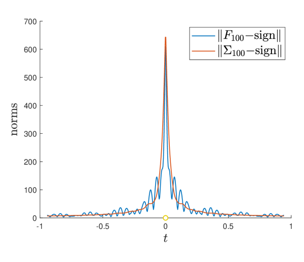
(b) nonsymmetric diagonalizable matrices

Figure 4. Matrix sign function approximated by matrix Fourier and Cesáro sums.

Outside $t=0$, where the matrix sign function is undefined, both $F_{100}$ and $\Sigma_{100}$ provide fair approximations as quantified by $\lVert F_{100}(Y(t))-\operatorname{sign}(Y(t))\rVert$ and $\lVert\Sigma_{100}(Y(t))-\operatorname{sign}(Y(t))\rVert$ in Figure 4. We expect the approximation errors to further decrease as the number of terms increases beyond $100$. For comparison the more accurate approximations in Figure 2(a) for the scalar series took a $1000$-term approximation, which is beyond our reach here for $1000\times 1000$ matrix series.

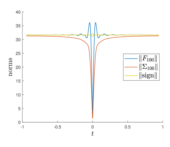
(a) symmetric matrices

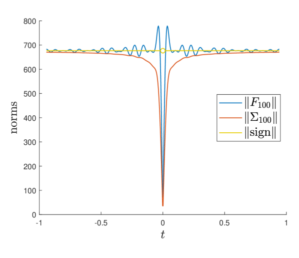
(b) nonsymmetric diagonalizable matrices

Figure 5. Gibbs phenomena in matrix Fourier series corrected with Cesáro sum.

In a neighborhood of $t=0$, we see the unmistakable mark of Gibbs phenomenon in $F_{100}$, reflected in the norms of $\lVert F_{100}(Y(t))\rVert$ and $\lVert F_{100}(Z(t))\rVert$, the blue curves in Figures 5(a) and 5(b) respectively. The oscillatory behavior vanishes when we instead look at the corresponding Cesáro sums $\Sigma_{100}$, whose norms are given by the red curves in Figure 5. This indicates that for diagonalizable matrices, Cesáro summation is a remedy for Gibbs phenomenon in matrix Fourier series.

8.2. Accurate summation with Euler method and strong Borel method

These experiments accomplish two goals. We first verify numerically that the Euler and strong Borel methods indeed extend the domain of Neumann series beyond $\mathbb{D}$, which we demonstrated analytically in Corollary 3.11 and Proposition 4.19. The experiments for Euler methods are also used to show that the Schur–Parlett algorithm for Euler summation, i.e., Algorithm 6 with $c_{n,k}=\binom{n+1}{k+1}\rho^{n-k}(1+\rho)^{-n-1}$, is less accurate but dramatically faster than directly computing with Algorithm 2.

We generate fifty matrices $X\in\mathbb{C}^{1000\times 1000}$ such that $\lambda(X)\subseteq\{z\in\mathbb{C}:\lvert z+\rho\rvert<1+\rho\}$ for $\rho=10^{4}$ and $\lambda(X)\not\subseteq\mathbb{D}$. Note that the Neumann series $\sum_{k=0}^{\infty}X^{k}$ for such matrices will not be conventionally summable. Our goal is to verify that Euler method and strong Borel method will however yield the expected $(I-X)^{-1}$ numerically. For Euler method, we compute the truncated $(\mathsf{E},\rho)$ sum as defined in (3.10),

$$\widehat{S}_{\scriptscriptstyle(\mathsf{E},{\rho})}\coloneqq\sum_{k=0}^{10000}\operatorname{\mathscr{E}}_{k}^{\rho}(X_{\bullet})$$

where $X_{\bullet}=(X^{k})_{k=0}^{\infty}$, first with compensated summation and then with the Schur–Parlett algorithm. For the strong Borel method, we use the Matlab function integral with tolerance level $10^{-12}$ to compute the Borel sum $\widehat{S}_{\scriptscriptstyle\mathsf{SB}}$ as in (4.7).

We plot the forward errors $\lVert\widehat{S}-(I-X)^{-1}\rVert$ in Figure 6 and the backward errors $\lVert\widehat{S}(I-X)-I\rVert$ in Figure 7, where $\widehat{S}$ is either $\widehat{S}_{\scriptscriptstyle(\mathsf{E},{\rho})}$ or $\widehat{S}_{\scriptscriptstyle\mathsf{SB}}$. The near zero errors are strong numerical evidence that both Euler and strong Borel methods analytically extend the Neumann series to $(I-X)^{-1}$, which we of course know is true by virtue of Corollary 3.11 and Proposition 4.19.

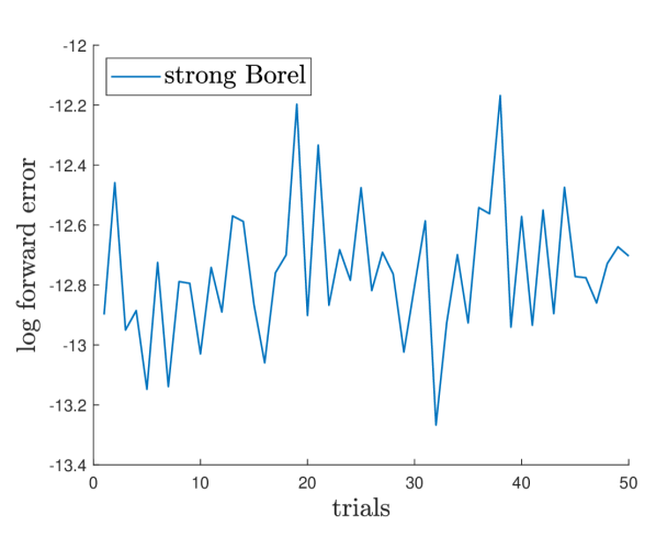
(a) strong Borel method

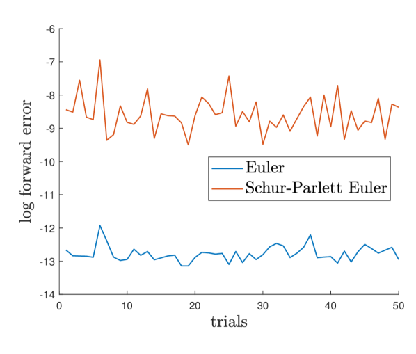
(b) Euler method

Figure 6. Log forward errors of strong Borel and Euler summations.

Observant readers might have noticed an issue here. We do not really have $(I-X)^{-1}$ exactly but only the output of the inv function in Matlab, which is also subjected to floating point and approximation errors. Indeed our ‘forward errors’ here are simply a measure of deviation from $\widehat{S}_{\texttt{inv}}$, the result of inv applied to $I-X$. The backward errors $\lVert\widehat{S}(I-X)-I\rVert$ for $\widehat{S}_{\texttt{inv}}$, $\widehat{S}_{\scriptscriptstyle(\mathsf{E},{\rho})}$, $\widehat{S}_{\scriptscriptstyle\mathsf{SB}}$ provide a more equitable comparison and therein lies a surprise — when computed with compensated summation, $\widehat{S}_{\scriptscriptstyle(\mathsf{E},{\rho})}$, the result of Euler method, is more accurate than $\widehat{S}_{\texttt{inv}}$, the result of Matlab’s inv, as is evident in Figure 7(b).

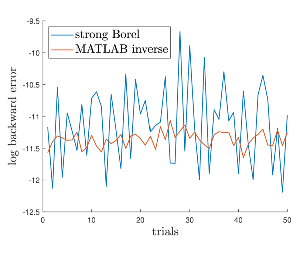
(a) strong Borel method

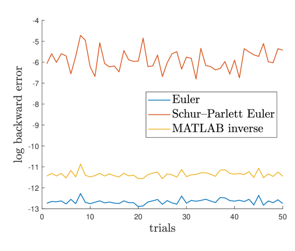
(b) Euler method

Figure 7. Log backward errors of strong Borel and Euler summations.

As both forward and backward errors in Figures 6(b) and 7(b) reveal, the Schur–Parlett algorithm gives less accurate results for Euler sums than compensated summation. However, a comparison of their running times in Figure 8 shows that the former is significantly faster.

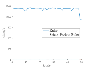
Figure 8. Run time comparison of compensated summation and Schur–Parlett algorithm on Euler sums.

8.3. High accuracy sums with Euler methods

The surprising accuracy of Euler method computed with compensated summation uncovered in Section 8.2 deserves a more careful look. Here we will examine how the value of $\rho$ impacts its accuracy.

We generate twenty bidiagonal matrices $X\in\mathbb{R}^{1000\times 1000}$ whose diagonal entries are negative with probability $\alpha\in\{0,0.01,\dots,0.99,1\}$. These matrices are generally not diagonalizable but we may readily prescribe their eigenvalue distribution. Again we will use the Neumann series $\sum_{k=0}^{\infty}X^{k}$, whose value $S=(I-X)^{-1}$ is known, as our test case. We approximate it with a $100$-term truncated Taylor series and a $100$-term Euler sum

$$\widehat{S}\coloneqq\sum_{k=0}^{100}X^{k}\quad\text{and}\quad\widehat{S}_{\scriptscriptstyle(\mathsf{E},{\rho})}\coloneqq\sum_{k=0}^{100}\operatorname{\mathscr{E}}_{k}^{\rho}(X_{\bullet}),$$

with $\rho\in\{1,1/2,1/4\}$, using compensated summation in Algorithm 2 to compute these sums. For a bidiagonal $X$ we know $S=(I-X)^{-1}$ exactly in closed form and do not need to rely on Matlab’s inv, we may compute the forward errors $\lVert\widehat{S}_{\scriptscriptstyle(\mathsf{E},{\rho})}-S\rVert$ and $\lVert\widehat{S}-S\rVert$. The logarithm of these values averaged over the twenty trials are plotted against $\alpha$ in Figure 9.

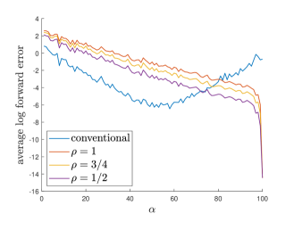
Figure 9. Log errors from Euler methods.

We highlight two observations. Firstly, the downward trend of the curves for Euler method with increasing $\alpha$ shows that when the eigenvalues are predominantly negative, a truncated Euler sum gives a much higher level of accuracy with $100$ terms than a truncated Taylor series with the same number of terms. This implies that Euler sums converge much faster than Taylor series. Secondly, when using Euler summation, smaller values of $\rho$ lead to faster convergence than larger ones.

8.4. Matrix Dirichlet series with Lambert summation

A Dirichlet series is a scalar series

$$\sum_{n=0}^{\infty}\frac{a_{n}}{n^{z}}$$

where $a_{\bullet}\in s(\mathbb{C})$ and $z$ is a complex variable. The best-known Dirichlet series is the Riemann zeta function

$$\zeta(z)=\sum_{n=1}^{\infty}\frac{1}{n^{z}}.$$

Another well-known Dirichlet series is one whose coefficients are given by $a_{n}=\mu(n)$, where

$$\mu(n)=\begin{dcases*}1&$n$ is square-free with an even number of prime factors,\\ -1&$n$ is square-free with an odd number of prime factors,\\ 0&$n$ is not square-free,\end{dcases*}$$

is the Möbius function. It turns out that for any $z\in\mathbb{C}$ with $\operatorname{Re}(z)>1$,

$$\sum_{n=1}^{\infty}\frac{\mu(n)}{n^{z}}=\frac{1}{\zeta(z)}$$

and

$$\lim_{z\to 1}\sum_{n=1}^{\infty}\frac{\mu(n)}{n^{z}}=0.$$ (8.5)

An important application of the scalar Lambert summation [35, Lemma 2.3.7] is to show that

$$\sum_{n=1}^{\infty}\frac{\mu(n)}{n}\mathrel{\overset{\scriptscriptstyle\mathsf{L}}{\leavevmode\resizebox{0.0pt}{0.0pt}{$=$}}}0$$ (8.6)

and our goal here is to verify a matrix analogue numerically.

It is straightforward to extend the definitions above. A matrix Dirichlet series is a matrix series

$$\sum_{n=0}^{\infty}a_{n}n^{-X}$$

where $X$ is a complex matrix variable that takes values in $\mathbb{C}^{d\times d}$ and

$$n^{X}\coloneqq\exp(\log(n)X),$$

with $\exp$ the matrix exponential function [24, Chapter 10]. Our numerical experiments show that if $X\in\mathbb{C}^{d\times d}$ has $\operatorname{Re}(X)\succeq I$, then

$$\sum_{n=1}^{\infty}\mu(n)n^{-X}$$ (8.7)

is Lambert summable in the sense of Definition 4.8 and

$$\lim_{X\to I}\biggl{(}\sum_{n=1}^{\infty}\mu(n)n^{-X}\biggr{)}\mathrel{\overset{\scriptscriptstyle\mathsf{L}}{\leavevmode\resizebox{0.0pt}{0.0pt}{$=$}}}0.$$ (8.8)

This is a matrix analogue of (8.5) and (8.6). Unlike the scalar version in (8.5), which is conventionally summable, our matrix version in (8.8) requires Lambert summation as the matrix Dirichlet series (8.7) is not conventionally summable if $1\in\lambda(X)$, but is nevertheless Lambert summable.

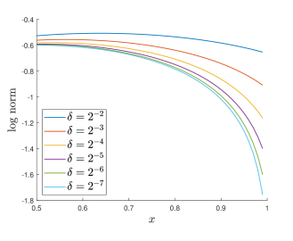
Figure 10. Lambert approximation of the Dirichlet series.

To verify (8.8) numerically, we generate random matrices $X\in\mathbb{C}^{1000\times 1000}$ with $\operatorname{Re}(X)\succeq I$ and $\lVert X-I\rVert=\delta$ for $\delta=2^{-2},2^{-3},\dots,2^{-7}$, and compute

$$\widehat{S}=(1-x)\sum_{n=1}^{10000}\frac{nx^{n}}{1-x^{n}}\mu(n)n^{-X}$$

to approximate the Lambert sum as $x\to 1^{-}$. As shown in Figure 10, for each $\delta$, $\lVert\widehat{S}\rVert$ approaches a limiting value as $x\to 1^{-}$, and $\lVert\widehat{S}\rVert\to 0$ as $\delta\to 0$ or, equivalently, $X\to I$.

8.5. Recursive versus compensated summations

We present two sets of experiments to compare recursive summation in (6.1) with compensated summation in Algorithm 2, focusing on how the errors scale with respect to series length and matrix dimensions.

For $X\in\mathbb{R}^{d\times d}$, we consider the $n$-term Neumann series

$$\sum_{k=0}^{n-1}X^{k}=(I-X^{n})(I-X)^{-1}\eqqcolon S$$ (8.9)

for fixed $n=1000$ and $d=1,\dots,1000$. We also consider its $n$-term Hadamard analogue, i.e., with power taken with respect to the Hadamard product

$$\sum_{k=0}^{n-1}X^{\circ k}=S_{\circ},\quad s_{ij}^{\circ}=\frac{1-x_{ij}^{n}}{1-x_{ij}},\quad i,j=1,\dots,d,$$ (8.10)

for fixed $d=1000$ and $n=1,\dots,5000$. In both cases we have the respective closed-form expressions for $S$ and $S_{\circ}$ on the right of (8.9) and (8.10) that give their exact values and thereby permit calculation of forward errors.

We compute $\widehat{S}$, the sum on the left of (8.9), and $\widehat{S}_{\circ}$ the sum on the left of (8.10) using both recursive summation in (6.1) and compensated summation in Algorithm 2. The forward errors $\lVert\widehat{S}-S\rVert_{\scriptscriptstyle\mathsf{F}}$ and $\lVert\widehat{S}_{\circ}-S_{\circ}\rVert_{\scriptscriptstyle\mathsf{F}}$ are shown in Figures 11(a) and 11(b) respectively. The result is clear: compensated summation is consistently more accurate than recursive summation, particularly with respect to increasing series length $n$, where the increase in errors follow significantly different trends.

While our forward error bound (6.5) predicts that the errors in compensated summation should be free of any dependence on $n$, this is assuming that we know the $k$th term exactly. In our sum (8.10), the $k$th term $X^{\circ k}$ is computed, and the increase in errors we see in Figure 11(b) is a result of the multiplication errors accumulating in $\widehat{S}_{\circ}$ as $n$ increases.

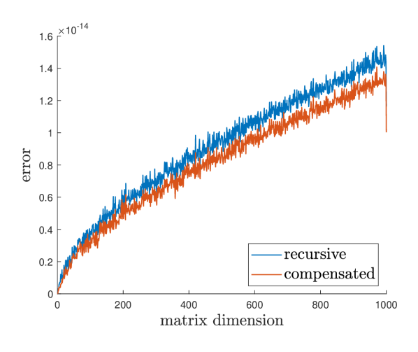
(a) increasing matrix dimension $d$

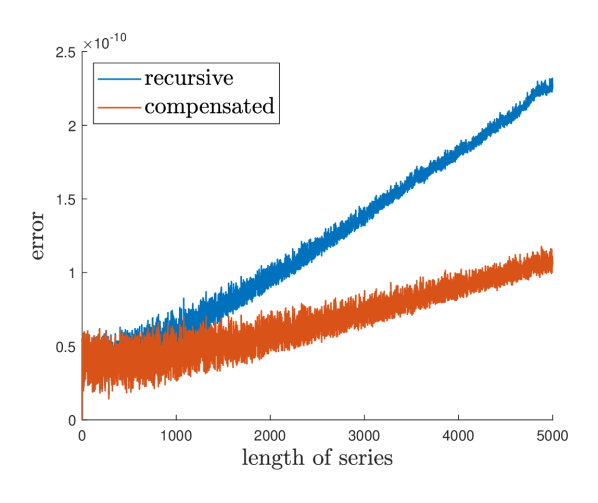
(b) increasing series length $n$

Figure 11. Errors for recursive and compensated summation algorithms.

In case the reader is wondering why we did two different sets of experiments with respect to standard and Hadamard products: Hadamard products will not reveal the dependence on $d$ in Figure 11(a) as they are computed entrywise; whereas standard products will result in the multiplicative errors masking the trend in Figure 11(b) showing dependence on $n$, as computing $X^{k}$ requires an order of magnitude more multiplications than computing $X^{\circ k}$.

9. Conclusion

This article is likely the first systematic study of summation techniques, both theoretical and numerical, for matrix series. Indeed we are unable to find much discussion of general numerical algorithms even for summing conventionally convergent matrix series, let alone the more convoluted summation methods for matrix series divergent in the conventional sense. The handful of previous works we found [12, 24, 25] had all focused on conventional summation of specific matrix Taylor series related to matrix functions, and said nothing of other summation methods or more general matrix series. Despite the length of our article, it still leaves significant room for future work, with several immediate open problems that we will briefly describe.

Our extensions of matrix Abelian mean in Definition 4.2, matrix Lambert sum in Definition 4.8, weak and strong matrix Borel sums in Definitions 4.10 and 4.12, leave open the question of whether one may further extend them by replacing the scalar parameter $x$ in these definitions by a positive definite matrix. One may also ask a similar question of the matrix Mittag-Leffler sum in Definition 4.13: Could the gamma function be replaced by the matrix gamma function [27]?

Another aspect beyond the scope of this article is that of conditioning, which likely explains the surprising accuracy of Euler method over matrix inversion uncovered in Section 8.2. Note that the left- and right-hand sides of (1.2), despite being equal in value, involve two different computational problems and almost surely have entirely different condition numbers. What is lacking is a study of the condition numbers of the summation methods in Sections 3 and 4.

The numerical methods in Sections 6 and 7 are mainly designed with accuracy in mind. They work well when adapted for matrix series and in conjunction with the summation methods in Sections 3 and 4. When it comes to speed, there are many acceleration methods for scalar series such as Aitken’s $\delta^{2}$-process and the vector $\varepsilon$-algorithm [9, 17, 39], but these involve nonlinear transforms and adapting them for matrix series is a challenge we save for the future.

As we alluded to in the introduction, these summation methods will allow for numerical investigations of “random matrix series,” one that has its $k$th term $A_{k}$ randomly generated according to some distributions like Wishart or GUE [6]. Many celebrated results in random matrix theory were indeed discovered first through numerical experiments and only rigorously proved much later.

Acknowledgments

This work is partially supported by the DARPA grant HR00112190040, the NSF grants DMS 1854831 and ECCS 2216912, and a Vannevar Bush Faculty Fellowship ONR N000142312863.

References

• [1] F. S. Acton. Numerical methods that work. Mathematical Association of America, Washington, DC, 1990. Corrected reprint of the 1970 edition.
• [2] R. Askey. Orthogonal polynomials and special functions. Society for Industrial and Applied Mathematics, Philadelphia, PA, 1975.
• [3] P. Blanchard, N. J. Higham, and T. Mary. A class of fast and accurate summation algorithms. SIAM J. Sci. Comput., 42(3):A1541–A1557, 2020.
• [4] J. Boos. Classical and modern methods in summability. Oxford Mathematical Monographs. Oxford University Press, Oxford, 2000. Assisted by Peter Cass, Oxford Science Publications.
• [5] E. Borel. Mémoire sur les séries divergentes. Ann. Sci. École Norm. Sup. (3), 16:9–131, 1899.
• [6] A. Borodin, I. Corwin, and A. Guionnet, editors. Random matrices, volume 26 of IAS/Park City Mathematics Series. American Mathematical Society, Providence, RI, 2019.
• [7] D. Borwein and B. L. R. Shawyer. On Borel-type methods. Tohoku Math. J. (2), 18:283–298, 1966.
• [8] D. W. Boyd. A $p$-adic study of the partial sums of the harmonic series. Experiment. Math., 3(4):287–302, 1994.
• [9] C. Brezinski and M. Redivo Zaglia. Extrapolation methods, volume 2 of Studies in Computational Mathematics. North-Holland Publishing Co., Amsterdam, 1991. Theory and practice, With 1 IBM-PC floppy disk (5.25 inch).
• [10] E. Cesàro. Sur la multiplication des series. Bull. Sci. Math., 14:114–120, 1890.
• [11] I. Coskun and E. Riedl. Normal bundles of rational curves in projective space. Math. Z., 288(3-4):803–827, 2018.
• [12] P. I. Davies and N. J. Higham. A Schur-Parlett algorithm for computing matrix functions. SIAM J. Matrix Anal. Appl., 25(2):464–485, 2003.
• [13] N. Dunford and J. T. Schwartz. Linear Operators. I. General Theory, volume Vol. 7 of Pure and Applied Mathematics. Interscience Publishers, Inc., New York; Interscience Publishers Ltd., London, 1958. With the assistance of W. G. Bade and R. G. Bartle.
• [14] L. Fejér. Untersuchungen über Fouriersche Reihen. Math. Ann., 58(1-2):51–69, 1903.
• [15] J. Glimm and A. Jaffe. Quantum physics. Springer-Verlag, New York, second edition, 1987. A functional integral point of view.
• [16] G. H. Golub and C. F. Van Loan. Matrix computations. Johns Hopkins Studies in the Mathematical Sciences. Johns Hopkins University Press, Baltimore, MD, third edition, 1996.
• [17] P. R. Graves-Morris, D. E. Roberts, and A. Salam. The epsilon algorithm and related topics. volume 122, pages 51–80. 2000. Numerical analysis 2000, Vol. II: Interpolation and extrapolation.
• [18] R. G. Gurau and T. Krajewski. Analyticity results for the cumulants in a random matrix model. Ann. Inst. Henri Poincaré D, 2(2):169–228, 2015.
• [19] E. Hairer and G. Wanner. Analysis by its history. Undergraduate Texts in Mathematics. Springer-Verlag, New York, 1996. Readings in Mathematics.
• [20] G. H. Hardy. Divergent series. Éditions Jacques Gabay, Sceaux, 1992. With a preface by J. E. Littlewood and a note by L. S. Bosanquet, Reprint of the revised (1963) edition.
• [21] G. H. Hardy and J. E. Littlewood. On a Tauberian Theorem for Lambert’s Series, and Some Fundamental Theorems in the Analytic Theory of Numbers. Proc. London Math. Soc. (2), 19(1):21–29, 1920.
• [22] S. W. Hawking. Zeta function regularization of path integrals in curved spacetime. Comm. Math. Phys., 55(2):133–148, 1977.
• [23] N. J. Higham. Accuracy and stability of numerical algorithms. Society for Industrial and Applied Mathematics (SIAM), Philadelphia, PA, second edition, 2002.
• [24] N. J. Higham. Functions of matrices. Society for Industrial and Applied Mathematics (SIAM), Philadelphia, PA, 2008. Theory and computation.
• [25] N. J. Higham. The scaling and squaring method for the matrix exponential revisited. SIAM Rev., 51(4):747–764, 2009.
• [26] E. Hille and J. D. Tamarkin. On the summability of Fourier series. I. Trans. Amer. Math. Soc., 34(4):757–783, 1932.
• [27] L. Jódar and J. C. Cortés. Some properties of gamma and beta matrix functions. Appl. Math. Lett., 11(1):89–93, 1998.
• [28] W. Kahan. Pracniques: Further remarks on reducing truncation errors. Commun. ACM, 8(1):40, jan 1965.
• [29] Y. Katznelson. An introduction to harmonic analysis. Cambridge Mathematical Library. Cambridge University Press, Cambridge, third edition, 2004.
• [30] K. Knopp. Theorie und Anwendung der Unendlichen Reihen. Springer-Verlag, Berlin-Heidelberg, 1947. 4th ed.
• [31] J. Korevaar. Tauberian theory, volume 329 of Grundlehren der mathematischen Wissenschaften [Fundamental Principles of Mathematical Sciences]. Springer-Verlag, Berlin, 2004. A century of developments.
• [32] L.-H. Lim. Tensors in computations. Acta Numer., 30:555–764, 2021.
• [33] Y. I. Manin. A course in mathematical logic for mathematicians, volume 53 of Graduate Texts in Mathematics. Springer, New York, second edition, 2010. Chapters I–VIII translated from the Russian by Neal Koblitz, With new chapters by Boris Zilber and the author.
• [34] R. Mathias. Approximation of matrix-valued functions. SIAM J. Matrix Anal. Appl., 14(4):1061–1063, 1993.
• [35] M. Mursaleen. Applied summability methods. SpringerBriefs in Mathematics. Springer, Cham, 2014.
• [36] N. E. Nörlund. Sur une application des fonctions permutables. Universitets Arsskrift, (N.F.), avd. 2, 16(3), 1920.
• [37] B. N. Parlett. A recurrence among the elements of functions of triangular matrices. Linear Algebra Appl., 14(2):117–121, 1976.
• [38] A. Peyerimhoff. Lectures on summability. Lecture Notes in Mathematics, Vol. 107. Springer-Verlag, Berlin-New York, 1969.
• [39] W. H. Press, S. A. Teukolsky, W. T. Vetterling, and B. P. Flannery. Numerical recipes in FORTRAN. Cambridge University Press, Cambridge, second edition, 1992. The art of scientific computing, With a separately available computer disk.
• [40] A. M. Robert. A course in $p$-adic analysis, volume 198 of Graduate Texts in Mathematics. Springer-Verlag, New York, 2000.
• [41] J. B. Rosser. Transformations to speed the convergence of series. J. Research Nat. Bur. Standards, 46:56–64, 1951.
• [42] W. Rudin. Principles of mathematical analysis. International Series in Pure and Applied Mathematics. McGraw-Hill Book Co., New York-Auckland-Düsseldorf, third edition, 1976.
• [43] B. N. Sahney. On the Nörlund summability of Fourier series. Pacific J. Math., 13:251–262, 1963.
• [44] B. Shawyer and B. Watson. Borel’s methods of summability. Oxford Mathematical Monographs. The Clarendon Press, Oxford University Press, New York, 1994. Theory and applications, Oxford Science Publications.
• [45] S. Weinberg. The quantum theory of fields. Vol. I. Cambridge University Press, Cambridge, 2005. Foundations.
• [46] N. Wiener. Tauberian theorems. Ann. of Math. (2), 33(1):1–100, 1932.
• [47] G. F. Woronoi. Extension of the notion of the limit of the sum of terms of an infinite series. Ann. of Math. (2), 33(3):422–428, 1932.
• [48] N. Young. An introduction to Hilbert space. Cambridge Mathematical Textbooks. Cambridge University Press, Cambridge, 1988.
• [49] F. Zhang. Matrix theory. Universitext. Springer, New York, second edition, 2011. Basic results and techniques.