Bilevel Reinforcement Learning
via the Development of Hyper-gradient without Lower-Level Convexity

Abstract

Bilevel reinforcement learning (RL), which features intertwined two-level problems, has attracted growing interest recently. The inherent non-convexity of the lower-level RL problem is, however, to be an impediment to developing bilevel optimization methods. By employing the fixed point equation associated with the regularized RL, we characterize the hyper-gradient via fully first-order information, thus circumventing the assumption of lower-level convexity. This, remarkably, distinguishes our development of hyper-gradient from the general AID-based bilevel frameworks since we take advantage of the specific structure of RL problems. Moreover, we propose both model-based and model-free bilevel reinforcement learning algorithms, facilitated by access to the fully first-order hyper-gradient. Both algorithms are provable to enjoy the convergence rate $\mathcal{O}\left({\epsilon^{-1}}\right)$. To the best of our knowledge, this is the first time that AID-based bilevel RL gets rid of additional assumptions on the lower-level problem. In addition, numerical experiments demonstrate that the hyper-gradient indeed serves as an integration of exploitation and exploration.

1 Introduction

Bilevel optimization, aiming to solve problems with a hierarchical structure, achieves success in a wide range of machine learning applications, e.g., hyper-parameter optimization [19, 20, 83], meta-learning [7], computer vision [49], neural architecture search [47, 78], adversarial training [77], reinforcement learning [32, 10, 69], data poisoning [54]. To address the bilevel optimization problems, a line of research has emerged recently [23, 48, 50, 38, 33, 40, 68, 31, 82]. Generally, the upper-level (resp. the lower-level) problem optimizes the decision taken by the leader (resp. the follower), which exhibits potential for handling complicated decision-making processes such as Markov decision processes (MDPs).

Reinforcement learning (RL) [75, 76] serves as an effective way of learning to make sequential decisions in MDPs, and has seen plenty of applications [70, 6, 59, 58, 74]. The central task of RL is to find the optimal policy that maximizes the expected cumulative rewards in an MDP. Bilevel RL enriches the framework of RL by considering a two-level problem: the follower solves a standard RL problem within an environment parameterized by the decision variable taken by the leader; meanwhile, the leader optimizes the decision variable based on the response policy from the lower level. Recently, bilevel RL has gained increasing attention in practice, including RL from human feedback, [14], inverse RL [8], and reward shaping [34].

In this paper, we focus on the bilevel reinforcement learning problem:

$$\begin{array}[]{cl}\min\limits_{x\in\mathbb{R}^{n}}&\phi(x):=f\left(x,\pi^{*}(x)\right)\\ \mathrm{s.\,t.}&\pi^{*}(x)\in\operatorname*{arg\,min}\limits_{\pi\in\Pi}g(x,\pi),\end{array}$$ (1)

where $\Pi$ is the policy set of interest, the upper-level function $f$ is defined on $\mathbb{R}^{n}\times\Pi$, the univariate function $\phi$ is called the hyper-objective, and the gradient of $\phi(x)$ is referred to as the hyper-gradient [63, 24, 11, 80] if it exists. The approximate implicit differentiation (AID) based method which resorts to the hyper-gradient has become flourishing recently [23, 37, 3, 16, 32, 52, 21]. Specifically, in each outer iteration of the AID-based method, one implements an inexact hyper-gradient descent step $x_{k+1}=x_{k}-\beta\widetilde{\nabla}\phi(x_{k})$, where the estimator $\widetilde{\nabla}\phi(x_{k})$ of the hyper-gradient is obtained with the help of a few inner iterations. We consider the extension of AID-based methods to the bilevel reinforcement learning problem (1). Note that AID-based methods depend on the lower-level strong convexity [39, 36, 45] or uniform Polyak–Łojasiewicz (PL) condition [35, 10] to ensure the existence of the hyper-gradient. However, the lower-level problem in (1)—always an RL problem—is inherently non-convex even with strongly-convex regularization [1, 41], and only the non-uniform PL condition has been established [57], which renders $\nabla\phi$ ambiguous, as stated in [69].

Recently, Chakraborty et al. [10] presented an AID-based bilevel RL framework, assuming that the lower-level problem satisfies the uniform PL condition and the Hessian non-singularity condition. Shen et al. [69] proposed a penalty-based bilevel RL method to bypass the requirement of lower-level convexity by constructing two penalty functions. The convergence rate relies on the penalty parameter $\lambda$ that is at least the order of ${\epsilon^{-0.5}}$. In this paper, we develop both model-based and model-free bilevel RL algorithms, which are provable and exhibit an enhanced convergence rate, without additional assumptions on the lower-lower problem; see Table 1 for a detailed comparison with the existing bilevel RL methods.

Table 1: Comparison among bilevel reinforcement learning algorithms.

Algorithm	Lower-level Assumpsion	Conv. Rate	Inner Iter.	Oracle
PARL [10]	PL + Non-singular Hessian	$\mathcal{O}(\epsilon^{-1})$	-	1st+2nd
PBRL [69]	No	$\mathcal{O}(\lambda\epsilon^{-1})$	$\mathcal{O}\left({\log{\lambda^{2}\epsilon^{-1}}}\right)$	1st
M-SoBiRL (this work)	No	$\mathcal{O}(\epsilon^{-1})$	$\mathcal{O}\left({1}\right)$	1st
SoBiRL (this work)	No	$\mathcal{O}(\epsilon^{-1})$	$\mathcal{O}\left({\log{\epsilon^{-1}}}\right)$	1st

Contributions.

The main contributions are summarized as follows.

Firstly, we characterize the hyper-gradient of bilevel RL problem via fully first-order information and unveil its properties by investigating the fixed point equation associated with the entropy-regularized RL problem [62, 22, 81], which extends the spirits in [15, 24, 25, 26].

Secondly, understanding the hyper-gradient enables us to construct its estimators, upon which we devise a model-based bilevel RL algorithm, M-SoBiRL, together with a model-free version, SoBiRL. Specifically, the implementation only requires first-order oracles, which circumvents complicated second-order queries in general AID-based bilevel methods. To the best of our knowledge, it is the first time that AID-based bilevel RL algorithms are proposed without additional assumptions on the lower-level problem.

Finally, we offer an analysis to illustrate the efficiency of amortizing the hyper-gradient approximation through outer iterations in M-SoBiRL, i.e., it enjoys the convergence rate $\mathcal{O}(\epsilon^{-1})$ with the inner iteration number $N=\mathcal{O}(1)$ independent of the solution accuracy $\epsilon$. In the model-free scenario, we also establish an enhanced convergence property; refer to Table 1 for detailed results. In addition, the favorable performance of the proposed SoBiRL is validated on the Atari game, which implies that the hyper-gradient is an aggregation of exploitation and exploration.

2 Related Works

The introduction to related bilevel optimization methods can be found in Appendix A.

Entropy-regularized reinforcement learning. The entropy regularization is commonly considered in RL community. Specifically, the goal of entropy-regularized RL is to maximize the expected reward augmented with the policy entropy, thereby boosting both task success and behavior stochasticity. It facilitates exploration and robustness [87, 28, 29], smoothens the optimization landscape [2], and enhances the convergence property [61, 9, 84, 41, 80, 43]. Moreover, the policy optimality condition under entropy-regularized setting is equivalent to the softmax temporal value consistency in [62]. Therefore, the term soft is prefixed to quantities in this scenario, also resonating with the concept in [75], where “soft” means that the policy ensures positive probabilities across all state-action pairs.

Bilevel reinforcement learning. Extensive reinforcement learning applications hold the bilevel structure, e.g., reward shaping [72, 86, 34, 17, 27], offline reward correction [44], preference-based RL [14, 42, 64, 69], apprenticeship learning [4], Stackleberg Games [18, 71, 69], etc. In terms of provable bilevel reinforcement learning frameworks, Chakraborty et al. [10] proposed a policy alignment algorithm demonstrating performance improvements, and Shen et al. [69] designed a penalty-based method. Nevertheless, the research related to the hyper-gradient in bilevel RL remains constrained.

3 Problem Formulation

In this section, we will introduce the setting of entropy-regularized Markov decision processes [79, 87, 62, 28], and the formulation of bilevel reinforcement learning. Moreover, two specific instances of bilevel RL are introduced. The notation is listed in Appendix B.

3.1 Entropy-regularized MDPs

Discounted infinite-horizon MDPs. An MDP is characterized by a tuple $\mathcal{M}_{\tau}=(\mathcal{S},\mathcal{A},P,r,\gamma,\tau)$ with $\mathcal{S}$ and $\mathcal{A}$ serving as the state space and the action space, respectively. In this paper, we restrict the focus to the tabular setting, where both $\mathcal{S}$ and $\mathcal{A}$ are finite, i.e., $\left|{\mathcal{S}}\right|<+\infty$ and $\left|{\mathcal{A}}\right|<+\infty$. Furthermore, $P\in\mathbb{R}^{\left|{\mathcal{S}}\right|\left|{\mathcal{A}}\right|\times\left|{\mathcal{S}}\right|}$ is the transition matrix with $P_{sas^{\prime}}=P(s^{\prime}|s,a)$ representing the transition probability from state $s$ to state $s^{\prime}$ under action $a$. The vector $r\in\mathbb{R}^{\left|{\mathcal{S}}\right|\left|{\mathcal{A}}\right|}$ specifies the reward $r_{sa}$ received when action $a$ is carried out at state $s$. Note that $\gamma\in(0,1)$ is the discount factor, adjusting the importance of immediate versus future reward, and the temperature parameter $\tau\geq 0$ balances regularization and reward.

Soft value function and Q-function. A policy $\pi\in\mathbb{R}^{\left|{\mathcal{S}}\right|\left|{\mathcal{A}}\right|}$ provides an action selection rule, that is, for any $s\in\mathcal{S},\ a\in\mathcal{A}$, $\pi_{sa}=\pi(a|s)$ is the probability of performing action $a$ at state $s$, and we denote $\pi_{s}\in\mathbb{R}^{\left|{\mathcal{A}}\right|}$ to be the corresponding distribution over $\mathcal{A}$ at state $s$, which means $\pi_{s}$ belongs to the probability simplex $\Delta(\mathcal{A}):=\{x\in\mathbb{R}^{\left|{\mathcal{A}}\right|}:x_{i}\geq 0,\ \sum_{i=1}^{\left|{\mathcal{A}}\right|}x_{i}=1\}$. Collecting $\pi_{s}$ over $s\in\mathcal{S}$ defines $\Delta^{\left|{\mathcal{S}}\right|}(\mathcal{A}):=\{\pi=(\pi_{s})_{s\in\mathcal{S}}\in\mathbb{R}^{\left|{\mathcal{S}}\right|\left|{\mathcal{A}}\right|}:\pi_{s}\in\Delta(\mathcal{A})\text{ for }s\in\mathcal{S}\}$ as the feasible set of policies. For simplicity, the above two sets are abbreviated as $\Delta$ and $\Delta^{\left|{\mathcal{S}}\right|}$, respectively. A policy $\pi$ induces a $P^{\pi}\in\mathbb{R}^{\left|{\mathcal{S}}\right|\times\left|{\mathcal{S}}\right|}$, measuring the transition probability from one state to another, i.e., $P^{\pi}_{ss^{\prime}}=\sum_{a}\pi_{sa}P_{sas^{\prime}}$. To promote stochasticity and discourage premature convergence to sub-optimal policies [2], it commonly resorts to the entropy function $h(\cdot)$,

$$h(\pi_{s}):=-\sum_{a\in\mathcal{A}}\pi_{sa}\log{\pi_{sa}},\ \text{ for }\pi_{s}\in\mathbb{R}_{+}^{\left|{\mathcal{A}}\right|}\cap\Delta,$$

where $\mathbb{R}_{+}^{m}=\{z\in\mathbb{R}_{+}^{m}:z_{i}>0\}$. Consequently, the soft value function $V^{\pi}\in\mathbb{R}^{\left|{\mathcal{S}}\right|}$ represents the expected discounted reward augmented with policy entropy, i.e.,

$$V^{\pi}_{s}:=\mathbb{E}\left[{\sum_{t=0}^{\infty}\gamma^{t}\left({r_{s_{t}a_{t}}+\tau h(\pi_{s_{t}})}\right)\ \Big{|}\ s_{0}=s,\pi,\mathcal{M}_{\tau}}\right],\ \text{ for }s\in\mathcal{S},$$

where the expectation is taken over the trajectory $(s_{0},a_{0}\sim\pi(\cdot|{s_{0}}),s_{1}\sim P(\cdot|s_{0},a_{0}),\ldots)$. Given the initial state distribution $\rho\in\mathbb{R}_{+}^{\left|{\mathcal{S}}\right|}\cap\Delta\left({{\mathcal{S}}}\right)$, the objective of RL is to find the optimal policy $\pi\in\Delta^{\left|{\mathcal{S}}\right|}$ that solves the problem:

$$\max_{\pi\in\Delta^{\left|{\mathcal{S}}\right|}}\ \ \ V^{\pi}(\rho):=\mathbb{E}_{s\sim\rho}\left[{V^{\pi}_{s}}\right]=\mathbb{E}\left[{\sum_{t=0}^{\infty}\gamma^{t}\left({r_{s_{t}a_{t}}+\tau h(\pi_{s_{t}})}\right)\ \Big{|}\ s_{0}\sim\rho,\pi,\mathcal{M}_{\tau}}\right].$$ (2)

The soft Q-function $Q^{\pi}\in\mathbb{R}^{\left|{\mathcal{S}}\right|\left|{\mathcal{A}}\right|}$ associated with policy $\pi$, couples with $V^{\pi}$ in the following fashion,

$$\forall(s,a)\in\mathcal{S}\times\mathcal{A}:\quad Q^{\pi}_{sa}\! =r_{sa}+\gamma\mathbb{E}_{s^{\prime}\sim P(\cdot|s,a)}\left[V^{\pi}_{s^{\prime}}\right],$$ (3)

$$\forall s\in\mathcal{S}:\quad V^{\pi}_{s} =\mathbb{E}_{a\sim\pi(\cdot|s)}\left[-\tau\log\pi(a|s)+Q^{\pi}_{sa}\right].$$

It is worth noting that the optimization problem (2) admits a unique optimal soft policy $\pi^{*}$ independent of $\rho$ [62]. The corresponding optimal soft value function (resp. optimal soft Q-function) is denoted by $V^{*}:=V^{\pi^{*}}$ (resp. $Q^{*}:=Q^{\pi^{*}}$). If necessary, we add a subscript to clarify the environment in which the policy is evaluated, e.g., $V^{\pi}_{\mathcal{M}_{\tau}}$ and $Q^{\pi}_{\mathcal{M}_{\tau}}$.

3.2 Bilevel reinforcement learning formulation

The single-level reinforcement learning task in  Section 3.1 trains an agent with fixed rewards. In contrast, this work considers the scenario where the reward function is parameterized by a decision variable, a task dubbed “policy alignment” in [10]. Generally, we parameterize the reward $r(x)\in\mathbb{R}^{\left|{\mathcal{S}}\right|\left|{\mathcal{A}}\right|}$ with $x\in\mathbb{R}^{n}$, which results in a parameterized MDP $\mathcal{M}_{\tau}(x)=(\mathcal{S},\mathcal{A},P,r(x),\gamma,\tau)$. In parallel with Section 3.1, given $\mathcal{M}_{\tau}(x)$, we define the soft value function $V^{\pi}(x)$, the soft Q-function $Q^{\pi}(x)$, the objective $V_{\mathcal{M}_{\tau}\left(x\right)}^{\pi}\left(\rho\right)$, the optimal soft policy $\pi^{*}(x)$, the optimal soft value-function $V^{*}(x)$, and the optimal soft Q-function $Q^{*}(x)$, associated with $x$.

Consequently, we formulate the bilevel reinforcement learning problem:

$$\begin{array}[]{cl}\min\limits_{x\in\mathbb{R}^{n}}&\phi(x):=f\left(x,\pi^{*}(x)\right)\\ \mathrm{s.\,t.}&\pi^{*}(x)=\operatorname*{arg\,min}\limits_{\pi\in\Delta^{\left|{\mathcal{A}}\right|}}-V_{\mathcal{M}_{\tau}\left(x\right)}^{\pi}\left(\rho\right),\end{array}$$ (4)

where the upper-level function $f$ is defined on $\mathbb{R}^{n}\times\mathbb{R}^{\left|{\mathcal{S}}\right|\left|{\mathcal{A}}\right|}$.

3.3 Applications of bilevel reinforcement learning

We introduce two examples unified in the formulation (4). To make a distinction between environments at two levels, we denote the upper-level MDP by $\bar{\mathcal{M}}_{\bar{\tau}}=\{\mathcal{S},\mathcal{A},\bar{P},\bar{r},\bar{\gamma},\bar{\tau}\}$ with an initial state distribution $\bar{\rho}$, and the lower-level MDP by $\mathcal{M}_{\tau}(x)$ with $\rho$.

Reward shaping. In reinforcement learning, the reward function acts as the guiding signal to motivate agents to achieve specified goals. However, in many cases, the rewards are sparse, which impedes the policy learning, or are partially incorrect, which leads to inaccurate policies. To this end, from the perspective of bilevel RL, it is advisable to shape an auxiliary reward function $r(x)$ at the lower level for efficient agent training, while maintaining the original environment at the upper level to align with the initial task evaluation [34], which is established as

$$\min_{x\in\mathbb{R}^{n}}-V_{\bar{\mathcal{M}}_{\bar{\tau}}}^{\pi^{*}\left(x\right)}\left(\bar{\rho}\right),\quad\mathrm{s.\,t.}\ \pi^{*}\left(x\right)=\operatorname*{arg\,min}_{\pi\in\Delta^{\left|{\mathcal{A}}\right|}}-V_{\mathcal{M}_{\tau}\left(x\right)}^{\pi}\left(\rho\right).$$

Reinforcement learning from human feedback (RLHF). The target of RLHF is to learn the intrinsic reward function that incorporates expert knowledge, from simple labels only containing human preferences. Drawing from the original framework [14], Chakraborty et al. [10] and Shen et al. [69] have formulated it in a bilevel form, which optimizes a policy under the parameterized $r(x)$ at the lower level, and adjusts $x$ to align the preference predicted by the reward model $r(x)$ with the true labels at the upper level.

$$\min\limits_{x\in\mathbb{R}^{n}}\mathbb{E}_{y,d_{1},d_{2}\sim\rho\left(d;\pi^{*}\left(x\right)\right)}\left[l_{h}\left(d_{1},d_{2},y;x\right)\right],\quad\mathrm{s.\,t.}\ \pi^{*}\left(x\right)=\operatorname*{arg\,min}\limits_{\pi\in\Delta^{\left|{\mathcal{A}}\right|}}-V_{\mathcal{M}_{\tau}\left(x\right)}^{\pi}\left(\rho\right),$$

where each trajectory $d_{i}=\{\left({s_{h}^{i},a_{h}^{i}}\right)\}_{h=0}^{H-1}$ ($i=1,2$) is sampled from the distribution $\rho\left({d;\pi^{*}(x)}\right)$ generated by the policy $\pi^{*}(x)$ in the upper-level $\bar{\mathcal{M}}_{\bar{\tau}}$, i.e.,

$$P(d_{i})=\bar{\rho}\left({s_{0}^{i}}\right)\left[{\Pi_{h=0}^{H-2}\pi^{*}(x)\left({a_{h}^{i}|s_{h}^{i}}\right)\bar{P}\left({s_{h+1}^{i}|s_{h}^{i},a_{h}^{i}}\right)}\right]\pi^{*}(x)\left({a_{H-1}^{i}|s_{H-1}^{i}}\right),$$

and the preference label $y\in\{0,1\}$, indicating preference for $d_{1}$ over $d_{2}$, obeys human feedback distribution $y\sim D_{human}(y|d_{1},d_{2})$. Moreover, $l_{h}$ is the binary cross-entropy loss,

$$l_{h}\left(d_{1},d_{2},y;x\right)=-y\log P\left(d_{1}\succ d_{2};x\right)-\left(1-y\right)\log P\left(d_{2}\succ d_{1};x\right),$$

with the preference probability $P\left({d_{1}\succ d_{2};x}\right)$ built by the Bradley–Terry model:

$$P\left(d_{1}\succ d_{2};x\right)=\frac{\exp\left(\sum_{h=0}^{H-1}{r_{s_{h}^{1},a_{h}^{1}}\left(x\right)}\right)}{\exp\left(\sum_{h=0}^{H-1}{r_{s_{h}^{1},a_{h}^{1}}\left(x\right)}\right)+\exp\left(\sum_{h=0}^{H-1}{r_{s_{h}^{2},a_{h}^{2}}\left(x\right)}\right)}.$$

4 Model-Based Soft Bilevel Reinforcement Learning

Addressing the bilevel RL problem (4) is challenging from two aspects: 1) analyzing the properties of $\pi^{*}(x)$, which has not been well studied but plays a crucial role in AID-based methods; 2) characterizing the hyper-gradient $\nabla\phi(x)$ which remains unclear. To this end, we take advantage of the specific structure of entropy-regularized RL to investigate $\pi^{*}(x)$ and identify $\nabla\phi(x)$. As a result, we propose a model-based algorithm to solve the bilevel RL problem (4).

Recall that the optimal soft quantities adhere to the following softmax temporal value consistency conditions [62]:

$$\forall(s,a)\in\mathcal{S}\times\mathcal{A}:\,\,\,\,\,\ \pi_{sa}^{*}(x) =\exp\left(\tau^{-1}\left({Q_{sa}^{*}\left(x\right)-V_{s}^{*}\left(x\right)}\right)\right)=\frac{\exp\left\{Q_{sa}^{*}\left(x\right)/\tau\right\}}{\sum_{a^{\prime}}{\exp\left(Q_{sa^{\prime}}^{*}\left(x\right)/\tau\right)}},$$ (5)

$$\forall s\in\mathcal{S}:\quad V_{s}^{*}\left(x\right) =\tau\log\left(\sum\nolimits_{a}{\exp\left(\frac{r_{sa}\left(x\right)+\gamma\sum_{s^{\prime}}{P_{sas^{\prime}}V_{s^{\prime}}^{*}\left(x\right)}}{\tau}\right)}\right)$$ (6)

$$=\tau\log\left(\sum\nolimits_{a}{\exp\left(Q_{sa}^{*}\left(x\right)/\tau\right)}\right).$$ (7)

By differentiating (5) and incorporating (3), we assemble $\{\nabla\pi_{sa}^{*}(x)\}$ in matrix form and obtain

$$\nabla\pi^{*}(x)={\tau^{-1}}\mathrm{diag}\left(\pi^{*}(x)\right)\left(\nabla r(x)-{U}\nabla V^{*}\left(x\right)\right)$$ (8)

with $U\in\mathbb{R}^{\left|{\mathcal{S}}\right|\left|{\mathcal{A}}\right|\times\left|{\mathcal{S}}\right|}$ defined by $U_{sas^{\prime}}:=1-\gamma P_{sas^{\prime}}$ for $s=s^{\prime}$ and $U_{sas^{\prime}}:=-\gamma P_{sas^{\prime}}$, otherwise. Hence, differentiating $\pi^{*}(x)$ boils down to considering the implicit differentiation $\nabla V^{*}(x)$. In view of (6), we notice that $V^{*}(x)$ is a fixed point related to the mapping $\varphi$,

$$\varphi(x,v):\ \ \mathbb{R}^{n}\times\mathbb{R}^{\left|{\mathcal{S}}\right|} \longrightarrow\mathbb{R}^{\left|{\mathcal{S}}\right|}$$

$$(x,v) \longmapsto\tau\log\left({\exp\left({\frac{r(x)+\gamma{P}v}{\tau}}\right)\cdot{\bf 1}}\right),$$

where $\log(\cdot)$ and $\exp(\cdot)$ are element-wise operations, and ${\bf 1}\in\mathbb{R}^{\left|{\mathcal{S}}\right|}$ is an all-ones vector. The structure of $\varphi(\cdot,\cdot)$, in consequence, can facilitate the characterization of $\nabla V^{*}(x)$, as outlined in the following proposition.

Proposition 4.1.

For any $x\in\mathbb{R}^{n}$, $\varphi(x,\cdot)$ is a contraction mapping, i.e., $\|\nabla_{v}\varphi(x,v)\|_{\infty}=\gamma<1$, and the matrix ${I-\nabla_{v}\varphi(x,v)}$ is invertible. Consequently, $V^{*}(x)$ is the unique fixed point of $\varphi(x,\cdot)$, with a well-defined derivative $\nabla V^{*}(x)$, given by

$$\nabla V^{*}(x)=\left({I-\nabla_{v}\varphi(x,V^{*}(x))}\right)^{-1}\nabla_{x}\varphi(x,V^{*}(x)).$$

Additionally, $\nabla_{v}\varphi\left({x,V^{*}(x)}\right)$ coincides with the $\gamma$-scaled transition matrix induced by the optimal soft policy $\pi^{*}(x)$, i.e.,

$$\nabla_{v}\varphi\left({x,V^{*}(x)}\right)=\gamma P^{\pi^{*}(x)}.$$

Combining the above proposition with (8), we identify the hyper-gradient $\nabla\phi(x)$ related to the problem (4),

$$\nabla\phi(x)= \ \nabla_{x}f(x,\pi^{*}(x))+\nabla\pi^{*}(x)^{\top}\nabla_{\pi}f(x,\pi^{*}(x))$$

$$= \ \nabla_{x}f(x,\pi^{*}(x))+\tau^{-1}\nabla r(x)^{\top}\operatorname{diag}\left({\pi^{*}(x)}\right)\nabla_{\pi}f(x,\pi^{*}(x))$$

$$-\tau^{-1}\nabla_{x}\varphi\left({x,V^{*}(x)}\right)^{\top}\left({I-\gamma P^{\pi^{*}(x)}}\right)^{-\top}U^{\top}\operatorname{diag}\left({\pi^{*}(x)}\right)\nabla_{\pi}f(x,\pi^{*}(x)).$$ (9)

In this manner, we unveil the hyper-gradient in the context of bilevel RL, by harnessing the softmax temporal value consistency and derivatives of a fixed-point equation.

Algorithm 1 Model-based soft bilevel reinforcement learning algorithm (M-SoBiRL)

0:  outer and inner iteration numbers $K,N$, step sizes $\beta,\xi$, initialization $x_{0},\pi_{0},Q_{0},w_{0}$

1:  for $k=1,\dots,K$ do

2:     $A_{k}=\left({I-\gamma P^{\pi_{k}}}\right)^{\top},\quad b_{k}=U^{\top}\operatorname{diag}\left({\pi_{k}}\right)\nabla_{\pi}f(x_{k},\pi_{k})$

3:     Compute $V_{k}$ by (10)

4:     $w_{k}=w_{k-1}-\xi\left({\left({A_{k}^{\top}A_{k}}\right)w_{k-1}-A_{k}^{\top}b_{k}}\right)$

5:     $x_{k+1}=x_{k}-\beta\widehat{\nabla}\phi\left(x_{k},\pi_{k},V_{k},w_{k}\right)$

6:     $Q_{k,0}=Q_{k}$

7:     for $n=1,\dots,N$ do

8:        $Q_{k,n}=\mathcal{T}_{\mathcal{M}_{\tau}(x_{k+1})}(Q_{k,n-1})$

9:     end for

10:     $Q_{k+1}=Q_{k,N}$, $\pi_{k+1}=\texttt{softmax}\left({Q_{k+1}/\tau}\right)$

11:  end for

11:  $(x_{K+1},\pi_{K})$

In light of the characterization (9), a model-based soft bilevel reinforcement learning algorithm, called M-SoBiRL, is proposed in Algorithm 1. In summary, the $k$-th outer iteration performs an inexact hyper-gradient descent step on $x_{k}$, with the aid of auxiliary iterates $\left({\pi_{k},Q_{k},V_{k},w_{k}}\right)$. Specifically, given $x_{k+1}$, the inner iterations aim to (approximately) solve the lower-level entropy-regularized MDP problem. To this end, the soft policy iteration studied by [29, 9] inspires us to define the following soft Bellman optimality operator $\mathcal{T}_{\mathcal{M}_{\tau}\left(x\right)}:\mathbb{R}^{\left|{\mathcal{S}}\right|\left|{\mathcal{A}}\right|}\to\mathbb{R}^{\left|{\mathcal{S}}\right|\left|{\mathcal{A}}\right|}$ associated with $x\in\mathbb{R}^{n}$,

$$\forall\ (s,a)\in\mathcal{S}\times\mathcal{A}:\quad\mathcal{T}_{\mathcal{M}_{\tau}\left(x\right)}(Q)(s,a)=r_{sa}(x)+\gamma\underset{s^{\prime}\sim P(\cdot\mid s,a)}{\mathbb{E}}\left[\tau\log\left(\left\|\exp\left(Q\left(s^{\prime},\cdot\right)/\tau\right)\right\|_{1}\right)\right].$$

Applying this operator iteratively leads to the optimal soft Q-value function, with a linear convergence rate in theory (see Section G.4). Therefore, $N$ inner iterations are invoked in line 7-9 of Algorithm 1 to estimate $Q^{*}\left({x_{k+1}}\right)$, and the warm-start strategy is adopted in line 10 of Algorithm 1 to initialize the next outer iteration with historical information, where it amortizes the computation of $Q^{*}(x)$ through the outer iterations. Additionally, in order to recover $\pi_{k+1}$ from $Q_{k+1}$, we take into account the consistency condition (5) which involves the softmax mapping as follows,

$$\texttt{softmax}:\ \ \mathbb{R}^{\left|{\mathcal{S}}\right|\left|{\mathcal{A}}\right|} \longrightarrow\mathbb{R}^{\left|{\mathcal{S}}\right|\left|{\mathcal{A}}\right|}$$

$$\theta \longmapsto\left({\frac{\exp\left(\theta\left(s,a\right)\right)}{\sum_{a^{\prime}}{\exp\left(\theta\left(s,a^{\prime}\right)\right)}}}\right)_{sa}.$$

It follows from (5) that $\pi_{k+1}=\texttt{softmax}\left({Q_{k+1}/\tau}\right)$. As for the approximation of the hyper-gradient (9) which requires an inverse matrix vector product, we denote

$$A_{k}=\left({I-\gamma P^{\pi_{k}}}\right)^{\top},\quad b_{k}=U^{\top}\operatorname{diag}\left({\pi_{k}}\right)\nabla_{\pi}f(x_{k},\pi_{k}),$$

and employ $w_{k}$ to track the quantity $A_{k}^{-1}b_{k}$ in a similar principle of amortization. Concretely, $w_{k}$ is regarded as the (approximate) solution of the least squares problem, $\min_{w\in\mathbb{R}^{\left|{\mathcal{S}}\right|}}\frac{1}{2}\left\|{A_{k}w-b_{k}}\right\|^{2}$, and implements one gradient descent step (line 4 of Algorithm 1) in each outer iteration. Furthermore, elements of $Q_{k}$ are assembled to estimate the soft value function:

$$\forall s\in\mathcal{S}:\quad V_{k}\left(s\right)=\tau\log\left(\sum\nolimits_{a}{\exp\left(Q_{k}\left(s,a\right)/\tau\right)}\right),$$ (10)

which complies with the form of (7). Finally, collecting the iterates $\left(x_{k},\pi_{k},V_{k},w_{k}\right)$ yields the model-based hyper-gradient estimator $\widehat{\nabla}\phi$ in line 5 of Algorithm 1, i.e.,

$$\widehat{\nabla}\phi\left(x_{k},\pi_{k},V_{k},w_{k}\right):=\nabla_{x}f\left(x_{k},\pi_{k}\right)+\frac{1}{\tau}{\nabla r(x_{k})}^{\top}\operatorname{diag}\left({\pi_{k}}\right)\nabla_{\pi}f(x_{k},\pi_{k})-\frac{1}{\tau}\nabla_{x}\varphi(x_{k},V_{k})^{\top}w_{k}.$$

5 Model-Free Soft Bilevel Reinforcement Learning

In many real-world applications, agents lack access to the accurate model $P$ of the environment, underscoring the need for efficient model-free algorithms [65, 66, 46, 61, 67, 29]. When $P$ is unknown, two obstacles appear from the hyper-gradient computation (9). Specifically, it explicitly relies on the black-box transition matrix $P$ to compute $\nabla V^{*}(x)$, i.e.,

$$\nabla V^{*}(x)=\left({I-\gamma P^{\pi^{*}(x)}}\right)^{-1}\nabla_{x}\varphi(x,V^{*}(x)),$$ (11)

and the computation (9) involves complicated large-scale matrix multiplications. To circumvent them, we demonstrate how to derive the hyper-gradient by an expectation, which allows us to estimate $\nabla\phi(x)$ via sampling fully first-order information. Following these developments, we offer a model-free soft bilevel reinforcement learning algorithm.

In the model-free scenario, we concentrate on the upper-level function

$$f\left(x,\pi\right)=\mathbb{E}_{d_{i}\sim\rho\left(d;\pi\right)}\left[l\left(d_{1},d_{2},...,d_{I};x\right)\right],$$ (12)

where each trajectory $d_{i}=\{\left({s_{h}^{i},a_{h}^{i}}\right)\}_{h=0}^{H-1}$ ($i=1,2,\ldots,I$) is sampled from the trajectory distribution $\rho\left({d;\pi^{*}(x)}\right)$ generated by the policy $\pi^{*}(x)$ in the upper-level $\bar{\mathcal{M}}_{\bar{\tau}}$, and $l(\cdot;x)$ associated with $x$ is a function of trajectories. Notice that it incorporates the applications in Section 3.3, with $I=1$, $H=1$, $l=Q^{\pi^{*}(x)}_{\bar{\mathcal{M}}_{\bar{\tau}}}\left({s_{0}^{1},a_{0}^{1}}\right)$ for reward shaping, and $I=2$, finite $H$, $l=\mathbb{E}_{y}\left[{l_{h}\left({d_{1},d_{2},y;x}\right)}\right]$ for RLHF.

We extend Proposition 4.1 to absorb the transition matrix $P$ in (11) into an expectation, with the result that the implicit differentiations $\nabla V^{*}(x)$ and $\nabla Q^{*}(x)$ can be estimated by sampling the reward gradient under the policy $\pi^{*}(x)$.

Proposition 5.1.

For any $x\in\mathbb{R}^{n}$, $s\in\mathcal{S}$, and $a\in\mathcal{A}$,

$$\nabla V_{s}^{*}(x) =\mathbb{E}\left[\sum_{t=0}^{\infty}\gamma^{t}\nabla r_{s_{t},a_{t}}(x)\ \Big{|}\ s_{0}=s,\pi^{*}(x),\mathcal{M}_{\tau}\left({x}\right)\right],$$

$$\nabla Q_{sa}^{*}(x) =\mathbb{E}\left[\sum_{t=0}^{\infty}\gamma^{t}\nabla r_{s_{t},a_{t}}(x)\ \Big{|}\ s_{0}=s,a_{0}=a,\pi^{*}(x),\mathcal{M}_{\tau}\left({x}\right)\right].$$

Nevertheless, it is still intractable to construct the ${\left|{\mathcal{S}}\right|\times n}$ matrix $\nabla V^{*}(x)$ based on the above element-wise calculation, not to mention the large-scale matrix multiplications in (9). To bypass these matrix computations, we resort to the “log probability trick” [75] and the consistency condition (5). The subsequent proposition confirms that we can evaluate the hyper-gradient by interacting with the environment and collecting fully first-order information.

Proposition 5.2 (Hyper-gradient).

The hyper-gradient $\nabla\phi(x)$ of the bilevel reinforcement learning problem (4) with upper-level function (12) can be computed by

$$\nabla\phi(x)= \ \mathbb{E}_{d_{i}\sim\rho\left(d;\pi^{*}\left(x\right)\right)}\left[\nabla l\left(d_{1},d_{2},...,d_{I};x\right)\right]$$ (13)

$$+\tau^{-1}\mathbb{E}_{d_{i}\sim\rho\left(d;\pi^{*}\left(x\right)\right)}\left[l\left(d_{1},d_{2},...,d_{I};x\right)\left(\sum_{i}{\sum_{h}{\nabla\left(Q_{s_{h}^{i}a_{h}^{i}}^{*}\left(x\right)-V_{s_{h}^{i}}^{*}\left(x\right)\right)}}\right)\right].$$ (14)

Essentially, the first term (13) in the hyper-gradient contributes to decreasing the upper-level function, and the second term (14) condenses the gradient information transmitted from the lower level. Aggregating these two directions constructs the hyper-gradient, and updating the upper-level variable $x$ along $-\nabla\phi(x)$ will lead to a first-order stationary point (see Theorem 6.6).

In line with the above propositions, to facilitate the $k$-th (inexact) hyper-gradient descent step, the construction of a hyper-gradient estimator $\widetilde{\nabla}\phi(x_{k},\pi_{k})$ is devided into two steps: 1) evaluating the implicit differentiations based on $\pi_{k}$,

$$\widetilde{\nabla}V_{s}(x_{k},\pi_{k}) =\mathbb{E}\left[\sum_{t=0}^{\infty}\gamma^{t}\nabla r_{s_{t},a_{t}}(x_{k})\ \Big{|}\ s_{0}=s,\pi_{k},\mathcal{M}_{\tau}\left({x_{k}}\right)\right],$$

$$\widetilde{\nabla}Q_{sa}(x_{k},\pi_{k}) =\mathbb{E}\left[\sum_{t=0}^{\infty}\gamma^{t}\nabla r_{s_{t},a_{t}}(x_{k})\ \Big{|}\ s_{0}=s,a_{0}=a,\pi_{k},\mathcal{M}_{\tau}\left({x_{k}}\right)\right];$$

2) absorbing these components into the upper-level sampling process induced by $\pi_{k}$,

$$\widetilde{\nabla}\phi(x_{k},\pi_{k})= \ \mathbb{E}_{d_{i}\sim\rho\left(d;\pi_{k}\right)}\left[\nabla l\left(d_{1},d_{2},...,d_{I};x_{k}\right)\right]$$ (15)

$$+\tau^{-1}\mathbb{E}_{d_{i}\sim\rho\left(d;\pi_{k}\right)}\left[l\left(d_{1},d_{2},...,d_{I};x_{k}\right)\left(\sum_{i}{\sum_{h}{\widetilde{\nabla}\left(Q_{s_{h}^{i}a_{h}^{i}}-V_{s_{h}^{i}}\right)\left({x_{k},\pi_{k}}\right)}}\right)\right].$$

Consequently, we propose a model-free soft bilevel reinforcement learning algorithm, called SoBiRL, which is outlined in Algorithm 2. In the $k$-th outer iteration, we search for an approximate optimal soft policy $\pi_{k}$ satisfying ${\left\|{{\pi}_{k}-\pi^{*}(x_{k})}\right\|^{2}_{2}\leq\epsilon}$, which can be achieved by executing $\mathcal{O}\left({\log\epsilon^{-1}}\right)$ iterations of the policy mirror descent algorithm [41, 84]. Then, we utilize $\widetilde{\nabla}\phi(x_{k},\pi_{k})$, whose estimation only involves first-order oracles, for an inexact hyper-gradient descent step.

Algorithm 2 Model-Free Soft Bilevel Reinforcement Learning Algorithm (SoBiRL)

0:  iteration number $K$, step size $\beta$, initialization $x_{1},\pi_{0}$, required accuracy $\epsilon$

1:  for $k=1,\dots,K$ do

2:     Solve the lower-level problem approximately with the initial guess $\pi_{k-1}$ to get ${\pi}_{k}$ such that $\left\|{{\pi}_{k}-\pi^{*}(x_{k})}\right\|_{2}^{2}\leq\epsilon$

3:     Compute the approximate hyper-gradient $\widetilde{\nabla}\phi(x_{k},\pi_{k})$

4:     Implement an inexact hyper-gradient descent step $x_{k+1}=x_{k}-\beta\widetilde{\nabla}\phi(x_{k},\pi_{k})$

5:  end for

5:  $(x_{K+1},\pi_{K+1})$

6 Theoretical Analysis

In this section, we prove global convergence and give the iteration complexity for the proposed algorithms. The analysis requires only the regularity conditions—specifically, boundedness and Lipschitz continuity—of the first-order information. This distinguishes from general AID-based methods, which require additional smoothness assumptions regarding second-order derivatives [23, 12, 39, 16, 38]. The properties of $\varphi$, $\pi^{*}(x)$, and $V^{*}(x)$ are outlined in Appendix F. Moreover, it is worth emphasizing that the analysis for M-SoBiRL is different from that for SoBiRL. Thus, we organize their properties and the detailed proofs in Appendix G and Appendix H.

Assumption 6.1.

In the model-based scenario (4), $f$ is continuously differentiable. The gradient $\nabla f(x,\pi)$ is $L_{f}$-Lipschitz continuous, i.e., for any $x_{1},x_{2}\in\mathbb{R}^{n},\pi_{1},\pi_{2}\in\Delta^{\left|{\mathcal{S}}\right|}$,

$$\left\|{\nabla f(x_{1},\pi_{1})-\nabla f(x_{2},\pi_{2})}\right\|\leq L_{f}\left({\left\|{x_{1}-x_{2}}\right\|_{2}+\left\|{\pi_{1}-\pi_{2}}\right\|_{\infty}}\right),$$

and $\left\|{\nabla_{\pi}f(x,\pi^{*}(x)}\right\|_{2}\leq C_{f\pi}$.

Assumption 6.2.

In the model-free scenario with upper-level function (12), $l(d_{1},d_{2},\ldots,d_{I};x)$ parameterized by $x$ is a function of $I$ trajectories, each consisting of $H$ steps. $l\left({d_{1},d_{2},\ldots,d_{I};x}\right)$ is bounded by $C_{l}$, i.e., $\left|{l\left({d_{1},d_{2},\ldots,d_{I};x}\right)}\right|\leq C_{l}$, and is continuously differentiable with respect to $x$. $l(d_{1},d_{2},\ldots,d_{I};x)$ is $L_{l}$-Lipschitz continuous, i.e., for any $x_{1},x_{2}\in\mathbb{R}^{n}$ and $\left({d_{1},d_{2},\ldots,d_{I}}\right)$,

$$\left\|{l(d_{1},d_{2},\ldots,d_{I};x_{1})-l(d_{1},d_{2},\ldots,d_{I};x_{2})}\right\|_{2}\leq L_{l}\left\|{x_{1}-x_{2}}\right\|_{2},$$

Moreover, $\nabla l(d_{1},d_{2},\ldots,d_{I};x)$ is $L_{l1}$-Lipschitz continuous, i.e., for any $x_{1},x_{2}\in\mathbb{R}^{n}$ and $\left({d_{1},d_{2},\ldots,d_{I}}\right)$,

$$\left\|{\nabla l(d_{1},d_{2},\ldots,d_{I};x_{1})-\nabla l(d_{1},d_{2},\ldots,d_{I};x_{2})}\right\|_{2}\leq L_{l1}\left\|{x_{1}-x_{2}}\right\|_{2}.$$

Assumptions 6.1 and 6.2 specify the requirements for the upper-level problems in model-based and model-free scenarios, respectively. Generally, the boundedness and Lipschitz continuity assumptions related to $f$ are standard in bilevel optimization [23, 37, 3, 13, 45].

Assumption 6.3.

For any $x\in\mathbb{R}^{n},\ (s,a)\in\mathcal{S}\times\mathcal{A}$, the reward is bounded by $C_{r}$, i.e., $\left|{r_{sa}(x)}\right|\leq C_{r}$, and the gradient is bounded by $C_{rx}$, i.e., $\left\|{\nabla r_{sa}(x)}\right\|_{2}\leq C_{rx}$. Additionally, $r_{sa}(x)$ is $L_{r}$-Lipschitz smooth, i.e., for any $x_{1},x_{2}\in\mathbb{R}^{n}$, $\left\|{\nabla r_{sa}(x_{1})-\nabla r_{sa}(x_{2})}\right\|_{2}\leq L_{r}\left\|{x_{1}-x_{2}}\right\|_{2}$.

This assumption on the parameterized reward function is common in RL [85, 1, 10, 69].

In the model-based scenario, the following theorem reveals that the proposed algorithm M-SoBiRL benefits from amortizing the hyper-gradient approximation in which it enjoys the $\mathcal{O}\left({\epsilon^{-1}}\right)$ convergence rate, and the inner iteration number $N$ can be selected as a constant independent of the accuracy $\epsilon$.

Theorem 6.4 (Model-based).

Under Assumptions 6.1 and 6.3, in Algorithm 1, we can choose constant step sizes $\beta,\xi$, and the inner iteration number $N\sim\mathcal{O}(1)$. Then the iterates $\{x_{k}\}$ satisfy

$$\frac{1}{K}\sum_{k=1}^{K}\left\|{\nabla\phi(x_{k})}\right\|_{2}^{2}=\mathcal{O}\left({\frac{1}{K}}\right).$$

Detailed parameter setting is referred to Theorem G.12.

Regarding the model-free scenario, coupled with Proposition 5.2, the next proposition marks a substantial development to clarify the Lipschitz property of the hyper-gradient.

Proposition 6.5.

Under Assumption 6.3, given $x_{1},x_{2}\in\mathbb{R}^{n}$, we have for any $s\in\mathcal{S}$, $a\in\mathcal{A}$,

$$\left\|\nabla Q_{sa}^{*}(x_{1})-\nabla Q_{sa}^{*}(x_{2})\right\|_{2}\leq L_{V1}\left\|x_{1}-x_{2}\right\|_{2},\quad\left\|\nabla V_{s}^{*}(x_{1})-\nabla V_{s}^{*}(x_{2})\right\|_{2}\leq L_{V1}\left\|x_{1}-x_{2}\right\|_{2},$$

and

$$\left\|{\nabla\phi(x_{1})-\nabla\phi(x_{2})}\right\|_{2}\leq L_{\phi}\left\|{x_{1}-x_{2}}\right\|_{2},$$

with $L_{V1}$ and $L_{\phi}$ specified in Propositions H.5 and H.6, respectively.

Theorem 6.6 (Model-free).

Under Assumptions 6.2 and 6.3 and given the accuracy $\epsilon$ in Algorithm 2, we can set the constant step size $\beta<\frac{1}{2L_{\phi}}$, then the iterates $\{x_{k}\}$ satisfy

$$\frac{1}{K}\sum_{k=1}^{K}{\left\|\nabla\phi\left(x_{k}\right)\right\|^{2}}\leq\frac{\phi\left(x_{1}\right)-\phi^{*}}{K\left(\frac{\beta}{2}-\beta^{2}L_{\phi}\right)}+\frac{1+2\beta L_{\phi}}{1-2\beta L_{\phi}}L^{2}_{\widetilde{\phi}}\ \epsilon\ ,$$

where $\phi^{*}$ is the minimum of $\phi(x)$, and $L_{\phi},\ L_{\widetilde{\phi}}$ are specified in Propositions H.6 and H.7, respectively.

Combined with Table 1, the convergence property in Theorem 6.6 implies that the proposed algorithm SoBiRL realizes better iteration complexity than PBRL [68] with the same computation cost at each outer and inner iteration. Moreover, SoBiRL attains the convergence rate of the same order as PARL [10], but only employs first-order oracles and gets rid of additional assumptions on the lower-level problem.

7 Experiment

In this section, we conduct an experiment on the Atari game, BeamRider from the Arcade Learning Environment (ALE) [5] to empirically validate the efficiency of the model-free algorithm, SoBiRL. The reward provided by ALE serves as the ground truth, and for each trajectory pair, preference is assigned to the trajectory with higher accumulated ground-truth reward. We compare SoBiRL with DRLHF [14] and a baseline algorithm SAC [29, 30]. Both SoBiRL and DRLHF adopt deep neural networks to predict rewards, while the baseline SAC receives ground-truth rewards for training. More experiment details and parameter settings are summarized in Appendix I.

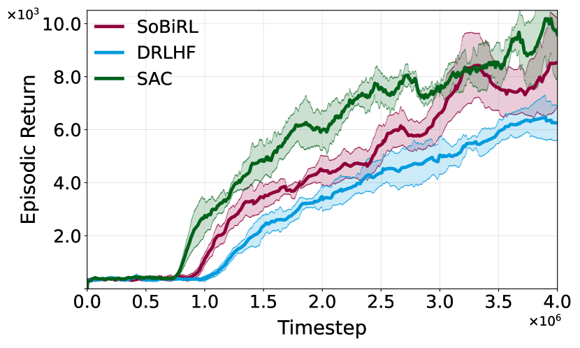
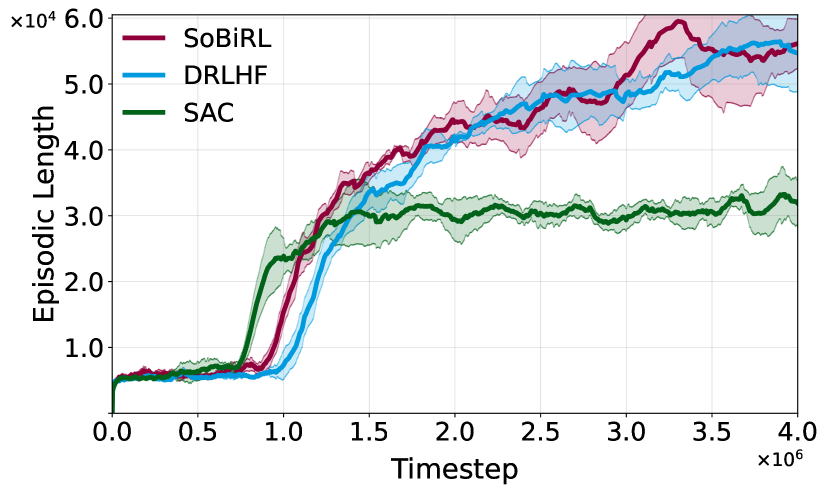
Figure 1: Comparison of algorithms on the Atari game, BeamRider, evaluated by the ground-truth reward. Both SoBiRL and DRLHF collect a total of $3000$ trajectory pairs. The running average over $15$ consecutive episodes is adopted for the presentation, and results are averaged over $5$ seeds.

The results are presented in Figure 1, showing that even in the face of unknown rewards, the performance of SoBiRL is on a par with the baseline SAC. Additionally, SoBiRL achieves a higher episodic return and a longer episodic life than DRLHF within the same outer timesteps. Another interesting observation is that, compared to the ground truth, the preference prediction based on the reward model of DRLHF achieves an accuracy of approximately $85\%$, while it hovers around $54\%$ with the reward model of SoBiRL. This stems from different update rules. Specifically, DRLHF alternates between learning a policy given the parameterized reward $r(x)$ and minimizing $\mathbb{E}\left[{l_{h}}\right]$ based on collecting trajectories, which decouples the task into two separate phases. It aligns preferences with the ground truth, but overlooks the exploration for rewards promoting better policy. Nevertheless, SoBiRL glues the two levels via the hyper-gradient ${\nabla}{\phi}$, with the first term (13) exploiting the preference information to align the reward predictor and the second term (14) exploring the implicit reward to unearth a more favorable policy. Therefore, SoBiRL produces superior results in reward prediction and policy optimization, although it may exhibit lower accuracy in alignment of trajectory preference.

Appendix

Appendix A Related Work in Bilevel Optimization

By the implicit function theorem, the approximate implicit differentiation (AID) based method regards the optimal lower-level solution as a function of the upper-level variable, which yields the hyper-gradient to instruct the upper-level update. It implements alternating (inexact) gradient descent steps between two levels [23, 37, 13, 16, 45, 32]. In addition, generalizing the lower-level strong convexity, the studies [24, 25, 26] focused on the bilevel problem where the lower-level problem is formulated as a fixed-point equation. Moreover, a line of research has been dedicated to the bilevel problem with a nonconvex lower-level objective [51, 68, 35, 56, 53]. Specifically, Shen and Chen [68] proposed a penalty-based method to bypass the requirement of lower-level convexity. In [35], a momentum-based approach was designed to solve the bilevel problem with a lower-level function satisfying the PL condition. Liu et al. [53] utilized the Moreau envelope based reformulation to provide a single-loop algorithm for nonconvex-nonconvex bilevel optimization.

Appendix B Vector and Matrix Notation

Throughout this paper, we adhere to the following conventions of vector and matrix notation.

• For any vector $q\in\mathbb{R}^{\left|{\mathcal{S}}\right|\left|{\mathcal{A}}\right|}$, we denote its component associated with $s\in\mathcal{S}$ as $q_{s}\in\mathbb{R}^{\left|{\mathcal{A}}\right|}$ or $q(s,\cdot)\in\mathbb{R}^{\left|{\mathcal{A}}\right|}$ in the following way,

  $$\forall\,(s,a)\in\mathcal{S}\times\mathcal{A},\quad q_{s}(a)=q(s,a)=q_{sa}.$$

  Additionally, for a vector $v\in\mathbb{R}^{\left|{\mathcal{S}}\right|}$, we use the notation of entry $v_{s}=v(s)$ interchangeably for convenience of exposition.

• $P\in\mathbb{R}^{\left|{\mathcal{S}}\right|\left|{\mathcal{A}}\right|\times\left|{\mathcal{S}}\right|}$, $r\in\mathbb{R}^{\left|{\mathcal{S}}\right|\left|{\mathcal{A}}\right|}$, $\pi\in\mathbb{R}^{\left|{\mathcal{S}}\right|\left|{\mathcal{A}}\right|}$: the transition matrix, the reward function, and the policy.

• $P^{\pi}\in\mathbb{R}^{\left|{\mathcal{S}}\right|\times\left|{\mathcal{S}}\right|}$: the transition matrix induced by $\pi$.

• $V^{\pi}\in\mathbb{R}^{\left|{\mathcal{S}}\right|}$, $Q^{\pi}\in\mathbb{R}^{\left|{\mathcal{S}}\right|\left|{\mathcal{A}}\right|}$: the soft value functions associated with $\pi$.

• $V^{*}(x)\in\mathbb{R}^{\left|{\mathcal{S}}\right|}$, $Q^{*}(x)\in\mathbb{R}^{\left|{\mathcal{S}}\right|\left|{\mathcal{A}}\right|}$, $\pi^{*}(x)\in\mathbb{R}^{\left|{\mathcal{S}}\right|\left|{\mathcal{A}}\right|}$: the optimal soft value functions and the optimal soft policy given $r(x)$.

• $\nabla\phi(x)\in\mathbb{R}^{n}$: the hyper-gradient.

• $\nabla_{x}\varphi(x,v)\in\mathbb{R}^{\left|{\mathcal{S}}\right|\times n}$, $\nabla_{v}\varphi(x,v)\in\mathbb{R}^{\left|{\mathcal{S}}\right|\times\left|{\mathcal{S}}\right|}$: the partial derivatives of $\varphi(x,v)$.

• $\nabla_{x}f(x,\pi)\in\mathbb{R}^{n}$, $\nabla_{\pi}f(x,\pi)\in\mathbb{R}^{\left|{\mathcal{S}}\right|\left|{\mathcal{A}}\right|}$: the partial derivatives of $f(x,\pi)$.

• $\nabla r(x)\in\mathbb{R}^{\left|{\mathcal{S}}\right|\left|{\mathcal{A}}\right|\times n}$: the derivative of $r(x)$.

• $\nabla V^{*}(x)\in\mathbb{R}^{\left|{\mathcal{S}}\right|\times n}$, $\nabla Q^{*}(x)\in\mathbb{R}^{\left|{\mathcal{S}}\right|\left|{\mathcal{A}}\right|\times n}$, $\nabla\pi^{*}(x)\in\mathbb{R}^{\left|{\mathcal{S}}\right|\left|{\mathcal{A}}\right|\times n}$: the implicit differentiations.

Appendix C Preliminaries on Numerical Linear Algebra

Proposition C.1.

Given a matrix $B\in\mathbb{R}^{m\times m}$ satisfying $\left\|{B}\right\|_{\infty}\leq\gamma$, then the matrix $I-B$ is invertible with the magnitudes of all its eigenvalues located within the interval $[1-\gamma,1+\gamma]$.

Proof.

Denote the entries of $B$ and $I-B$ by $\{b_{ij}\}_{i.j=1}^{m}$ and $\{l_{ij}\}_{i.j=1}^{m}$, respectively. Set $\lambda\in\mathbb{C}$ as an eigenvalue of $I-B$, and consider the Gershgorin circle theorem, for $i=1,2,\ldots,m$,

$$\left|{\lambda-l_{ii}}\right|\leq\sum_{j=1,j\neq i}^{m}\left|{l_{ij}}\right|.$$ (16)

Incorporating $l_{ii}=1-b_{ii}$ and $l_{ij}=-b_{ij}$ into (16), we obtain

$$\left|{\lambda-\left({1-b_{ii}}\right)}\right|\leq\sum_{j=1,j\neq i}^{m}\left|{b_{ij}}\right|,$$

The absolute value inequality leads to

$$-\sum_{j=1,j\neq i}^{m}\left|{b_{ij}}\right|\leq\left|{\lambda-1}\right|-\left|{b_{ii}}\right|\leq\sum_{j=1,j\neq i}^{m}\left|{b_{ij}}\right|,$$

which completes the proof since

$$\max_{i=1,2,\ldots,m}\sum_{j=1}^{m}\left|{b_{ij}}\right|=\left\|{B}\right\|_{\infty}=\gamma.$$

∎

Definition C.2.

A matrix $P\in\mathbb{R}^{m\times m}=(p_{ij})$ is defined to be a transition matrix if all entries are non-negative and each row sums to $1$, i.e., for any $i=1,2,\ldots,m$,

$$\sum_{j}p_{ij}=1.$$

Proposition C.3.

A transition matrix $P\in\mathbb{R}^{m\times m}=(p_{ij})$ always has an eigenvalue of $1$, while all the remaining eigenvalues have absolute values less than or equal to $1$.

Definition C.4.

A matrix $X=(x_{ij})\in\mathbb{R}^{m\times m}$ is called non-negative if all the entries are equal to or greater than zero, i.e.,

$$x_{ij}\geq 0,\ \text{ for }1\leq i,j\leq m.$$

Definition C.5.

A matrix $A\in\mathbb{R}^{m\times m}$ is an $M$-matrix if it can be expressed in the form $A=\mu I-B$, where $B=\left(b_{ij}\right)$ is non-negative, and $\mu\geq 0$ is equal to or greater than the moduli of any eigenvalue of $B$.

Proposition C.6.

Given a constant $\gamma\in(0,1)$ and a transition matrix $P\in\mathbb{R}^{m\times m}=(p_{ij})$, then the matrix $A=I-\gamma P$ is an $M$-matrix with the moduli of every eigenvalue in $[1-\gamma,1+\gamma]$, Additionally, the inverse of $A$ is

$$A^{-1}=\sum_{t=0}^{\infty}\gamma^{t}P^{t},$$

which is a non-negative matrix and holds all diagonal entries greater than or equal to $1$.

Proof.

Combined with Definition C.2 which reveals $\left\|{P}\right\|_{\infty}=1$ and Proposition C.1, it follows that any $\lambda\in\mathbb{C}$ as an eigenvalue of $A$ satisfies $\left|{\lambda}\right|\in[1-\gamma,1+\gamma]$, yielding that $A$ is invertible. Since ${\rho(\gamma P)=\gamma<1}$ by Proposition C.3, the infinite series $\sum_{t=0}^{\infty}\gamma^{t}P^{t}$ converges and coincides with the inverse of $A$, that is,

$$A^{-1}=\sum_{t=0}^{\infty}\gamma^{t}P^{t}.$$ (17)

Coupled with $P$ being non-negative and $\left({\gamma P}\right)^{0}=I$, (17) implies that $A^{-1}$ is non-negative with all diagonal entries greater than or equal to $1$. ∎

The next proposition serves as a technical tool in the later analysis.

Proposition C.7.

For any $\pi_{1},\pi_{2}\in\mathbb{R}_{+}^{\mathbb{\left|{\mathcal{S}}\right|\left|{\mathcal{A}}\right|}}\cap\Delta^{\left|{\mathcal{S}}\right|}$, the vector norms satisfy

$$\left\|{\pi_{1}-\pi_{2}}\right\|_{\infty} \leq\left\|{\log\pi_{1}-\log\pi_{2}}\right\|_{\infty},$$

$$\left\|{\pi_{1}-\pi_{2}}\right\|_{2} \leq\left\|{\log\pi_{1}-\log\pi_{2}}\right\|_{2}.$$

Proof.

It suffices to show for any $0<a,b<1$, $\left|{a-b}\right|\leq\left|{\log a-\log b}\right|$. Without loss of generality, suppose that $0<b\leq a<1$. Consider the function $G\left(z\right):=z-\log z$, with the derivative

$$G^{\prime}\left(z\right)=1-\frac{1}{z}<0,\quad\text{for}\ z\in(0,1),$$

which means $G(z)$ is monotonically decreasing on $(0,1)$. It leads to $a-\log a\leq b-\log b$, equivalently, $a-b\leq\log a-\log b$. ∎

Appendix D Proof in Section 4

The structure of $\varphi(\cdot,\cdot)$ facilitates the characterization of $\nabla V^{*}(x)$, as outlined in the following proposition.

Proposition D.1.

For any $x\in\mathbb{R}^{n}$, $\varphi(x,\cdot)$ is a contraction map, i.e., $\|\nabla_{v}\varphi(x,v)\|_{\infty}=\gamma<1$, and the matrix ${I-\nabla_{v}\varphi(x,v)}$ is invertible. Consequently, $V^{*}(x)$ is the unique fixed point of $\varphi(x,\cdot)$, with a well-defined derivative $\nabla V^{*}(x)$, given by

$$\nabla V^{*}(x)=\left({I-\nabla_{v}\varphi(x,V^{*}(x))}\right)^{-1}\nabla_{x}\varphi(x,V^{*}(x)).$$ (18)

Additionally, $\nabla_{v}\varphi\left({x,V^{*}(x)}\right)$ coincides with the $\gamma$-scaled transition matrix induced by the optimal soft policy $\pi^{*}(x)$, i.e.,

$$\nabla_{v}\varphi\left({x,V^{*}(x)}\right)=\gamma P^{\pi^{*}(x)}.$$ (19)

Proof.

Consider the mapping $F:\mathbb{R}^{n}\times\mathbb{R}^{\left|{\mathcal{S}}\right|}\to\mathbb{R}^{\left|{\mathcal{S}}\right|}$ defined by

$$F(x,v):=v-\varphi(x,v).$$

Then the partial derivative of $F(x,v)$ with respect to $v$ reads $I-\nabla_{v}\varphi(x,v)$. Computing

$$\left(\nabla_{v}\varphi\left(x,v\right)\right)_{ss^{\prime}}=\frac{\partial\varphi_{s}\left(x,v\right)}{\partial v_{s^{\prime}}}=\gamma\frac{\sum_{a}{P_{sas^{\prime}}\exp\left(\tau^{-1}\left(r_{sa}\left(x\right)+\gamma\sum_{s^{\prime\prime}}{P_{sas^{\prime\prime}}v_{s^{\prime\prime}}}\right)\right)}}{\sum_{a}{\exp\left(\tau^{-1}\left(r_{sa}\left(x\right)+\gamma\sum_{s^{\prime\prime}}{P_{sas^{\prime\prime}}v_{s^{\prime\prime}}}\right)\right)}}$$ (20)

leads to

$$\left\|{\nabla_{v}\varphi(x,v)}\right\|_{\infty}=\max_{s}\sum_{s^{\prime}}{\left|\left(\nabla_{v}\varphi\left(x,v\right)\right)_{ss^{\prime}}\right|}=\max_{s}\sum_{s^{\prime}}\frac{\gamma\sum_{a}P_{ass^{\prime}}\exp\left(\tau^{-1}\left(r^{x}_{sa}+\gamma\sum_{s^{\prime\prime}}P_{ass^{\prime\prime}}v_{s^{\prime\prime}}\right)\right)}{\sum_{a}\exp\left(\tau^{-1}\left(r^{x}_{sa}+\gamma\sum_{s^{\prime\prime}}P_{ass^{\prime\prime}}v_{s^{\prime\prime}}\right)\right)}=\gamma,$$

which means for any $x\in\mathbb{R}^{n}$, $\varphi(x,\cdot)$ is a contraction mapping, admiting a unique $V^{*}(x)$ such that $F(x,V^{*}(x))=0$. Additionally, by applying Proposition C.1, we can derive that $\nabla_{v}F(x,v)$ is invertible for any $(x,v)\in\mathbb{R}^{n}\times\mathbb{R}^{\left|{\mathcal{S}}\right|}$. Consequently, the implicit function theorem implies that there exists a differentiable function $V^{*}:\mathbb{R}^{n}\to\mathbb{R}^{\left|{\mathcal{S}}\right|}$ such that, for any $v\in\mathbb{R}^{\left|{\mathcal{S}}\right|}$ and $x\in\mathbb{R}^{n}$,

$$F(x,V^{*}(x))=V^{*}(x)-\varphi(x,V^{*}(x))={\bf 0},$$

with the derivative $\nabla V^{*}(x)$ satisfying

$$\nabla V^{*}(x)-\nabla_{x}\varphi(x,V^{*}(x))-\nabla_{v}\varphi(x,V^{*}(x))\nabla V^{*}(x)={\bf 0}.$$

Rearranging this yields the result (18). On the other hand, take (20) at $\left({x,V^{*}(x)}\right)$,

$$\left(\nabla_{v}\varphi\left(x,v\right)\right)_{ss^{\prime}}|_{v=V^{*}\left(x\right)} =\gamma\frac{\sum_{a}{P_{sas^{\prime}}\exp\left(\tau^{-1}\left(r_{sa}\left(x\right)+\gamma\sum_{s^{\prime\prime}}{P_{sas^{\prime\prime}}V_{s^{\prime\prime}}^{*}\left(x\right)}\right)\right)}}{\sum_{a}{\exp\left(\tau^{-1}\left(r_{sa}\left(x\right)+\gamma\sum_{s^{\prime\prime}}{P_{sas^{\prime\prime}}V_{s^{\prime\prime}}^{*}\left(x\right)}\right)\right)}}$$

$$=\gamma\frac{\sum_{a}{P_{sas^{\prime}}\exp\left(\tau^{-1}Q_{sa}^{*}\left(x\right)\right)}}{\exp\left(\tau^{-1}V_{s}^{*}\left(x\right)\right)}$$ (21)

$$=\gamma\sum_{a}{P_{sas^{\prime}}\exp\left(\tau^{-1}\left(Q_{sa}^{*}\left(x\right)-V_{s}^{*}\left(x\right)\right)\right)}$$

$$=\gamma\sum_{a}{P_{sas^{\prime}}\pi_{sa}^{*}\left(x\right)},$$ (22)

where (21) comes from (3) and (6), and (22) follows considering (5). Consequently, revisiting the definition of $P^{\pi^{*}(x)}$ yields the conclusion $\nabla_{v}\varphi\left({x,V^{*}(x)}\right)=\gamma P^{\pi^{*}(x)}$. ∎

Appendix E Proofs in Section 5

In this section, we provide proofs of the propositions in Section 5. The following proposition indicates that the implicit differentiations $\nabla V^{*}(x)$ and $\nabla Q^{*}(x)$ can be estimated by sampling the reward gradient under the policy $\pi^{*}(x)$.

Proposition E.1.

For any $x\in\mathbb{R}^{n}$, $s\in\mathcal{S}$, and $a\in\mathcal{A}$,

$$\nabla V_{s}^{*}(x) =\mathbb{E}\left[\sum_{t=0}^{\infty}\gamma^{t}\nabla r_{s_{t},a_{t}}(x)\ \Big{|}\ s_{0}=s,\pi^{*}(x),\mathcal{M}_{\tau}\left({x}\right)\right],$$

$$\nabla Q_{sa}^{*}(x) =\mathbb{E}\left[\sum_{t=0}^{\infty}\gamma^{t}\nabla r_{s_{t},a_{t}}(x)\ \Big{|}\ s_{0}=s,a_{0}=a,\pi^{*}(x),\mathcal{M}_{\tau}\left({x}\right)\right].$$

Proof.

Compute the partial derivative

$$\frac{\partial\varphi_{s}\left(x,v\right)}{\partial x_{i}}=\frac{\sum_{a}{\partial_{x_{i}}r_{sa}\left(x\right)\exp\left(\tau^{-1}\left(r_{sa}\left(x\right)+\gamma\sum_{s^{\prime\prime}}{P_{sas^{\prime\prime}}v_{s^{\prime\prime}}}\right)\right)}}{\sum_{a}{\exp\left(\tau^{-1}\left(r_{sa}\left(x\right)+\gamma\sum_{s^{\prime\prime}}{P_{sas^{\prime\prime}}v_{s^{\prime\prime}}}\right)\right)}},$$

and substitute $v=V^{*}(x)$ into it,

$$\nabla_{x}\varphi_{s}\left(x,V^{*}\left(x\right)\right)=\sum_{a}{\nabla r_{sa}\left(x\right)\pi_{sa}^{*}\left(x\right)},$$ (23)

where we adopt the similar derivation as (22). Applying Proposition C.6 to (19), we obtain

$$\left(I-\nabla_{v}\varphi\left(x,V^{*}\left(x\right)\right)\right)^{-1}=\sum_{t=0}^{\infty}{\left(\gamma P^{\pi^{*}\left(x\right)}\right)^{t}}.$$ (24)

Employ the subscript $s\in\mathcal{S}$ to denote the corresponding row of a matrix. It follows from (18), (23) and (24) that

$$\nabla V_{s}^{*}\left(x\right)= \left(I-\nabla_{v}\varphi\left(x,V^{*}(x)\right)\right)_{s}^{-1}\nabla_{x}\varphi\left(x,V^{*}\left(x\right)\right)$$

$$= \sum_{t=0}^{\infty}{\left(\gamma P^{\pi^{*}\left(x\right)}\right)_{s}^{t}}\nabla_{x}\varphi\left(x,V^{*}\left(x\right)\right)$$

$$= \sum_{t=0}^{\infty}{\gamma^{t}\sum_{s^{\prime}}{P\left(s_{t}=s^{\prime}|s_{0}=s,\pi^{*}\left(x\right)\right)}}\sum_{a}{\nabla r_{s^{\prime}a}\left(x\right)\pi_{s^{\prime}a}^{*}\left(x\right)}$$

$$= \sum_{t=0}^{\infty}{\gamma^{t}}\sum_{s^{\prime},a}{P\left(s_{t}=s^{\prime},a_{t}=a|s_{0}=s,\pi^{*}\left(x\right)\right)\nabla r_{s^{\prime}a}\left(x\right)}$$

$$= \ \mathbb{E}\left[\sum_{t=0}^{\infty}{\gamma^{t}\nabla_{x}r_{s_{t}a_{t}}\left(x\right)}\,\,|s_{0}=s,\pi^{*}\left(x\right),\mathcal{M}_{\tau}\left(x\right)\right],$$

where $P\left(s_{t}=s^{\prime},a_{t}=a|s_{0}=s,\pi^{*}\left(x\right)\right)$ is the probability of taking action $a$ at state $s^{\prime}$ at time $t$, given that the process starts from state $s_{0}=s$ in the MDP $\mathcal{M}_{\tau}(x)$. Differentiating both sides of

$$Q_{sa}^{*}\left(x\right)=r_{sa}\left(x\right)+\gamma\sum_{s^{\prime}}{P_{sas^{\prime}}V_{s^{\prime}}^{*}\left(x\right)}$$

with respect to $x$, we have

$$\nabla Q_{sa}^{*}\left(x\right)= \nabla r_{sa}\left(x\right)+\gamma\sum_{s^{\prime}}{P_{sas^{\prime}}\nabla V_{s^{\prime}}^{*}\left(x\right)}$$

$$= \ \mathbb{E}\left[\sum_{t=0}^{\infty}{\gamma^{t}\nabla_{x}r_{s_{t}a_{t}}\left(x\right)}\,\,|s_{0}=s,a_{0}=a,\pi^{*}\left(x\right),\mathcal{M}_{\tau}\left(x\right)\right].$$

∎

Subsequently, the next proposition characterizes the hyper-gradient via fully first-order information.

Proposition E.2.

The hyper-gradient $\nabla\phi(x)$ of the bilevel reinforcement learning problem (4) with the upper-level function (12) can be computed by

$$\nabla\phi(x)= \ \mathbb{E}_{d_{i}\sim\rho\left(d;\pi^{*}\left(x\right)\right)}\left[\nabla l\left(d_{1},d_{2},...,d_{I};x\right)\right]$$

$$+\tau^{-1}\mathbb{E}_{d_{i}\sim\rho\left(d;\pi^{*}\left(x\right)\right)}\left[l\left(d_{1},d_{2},...,d_{I};x\right)\left(\sum_{i}{\sum_{h}{\nabla\left(Q_{s_{h}^{i}a_{h}^{i}}^{*}\left(x\right)-V_{s_{h}^{i}}^{*}\left(x\right)\right)}}\right)\right].$$

Proof.

Recall that

$$P(d_{i};\pi^{*}\left(x\right))=\bar{\rho}\left({s_{0}^{i}}\right)\left[{\Pi_{h=0}^{H-2}\pi^{*}_{s_{h}^{i},a_{h}^{i}}\left(x\right)\bar{P}\left({s_{h+1}^{i}|s_{h}^{i},a_{h}^{i}}\right)}\right]\pi^{*}_{s_{H-1}^{i},a_{H-1}^{i}}(x),$$

and

$$\phi(x)=\mathbb{E}_{d_{i}\sim\rho\left(d;\pi^{*}\left(x\right)\right)}\left[l\left(d_{1},d_{2},...,d_{I};x\right)\right]=\sum_{\left(d_{1},...,d_{I}\right)}{l\left(d_{1},d_{2},...,d_{I};x\right)\Pi_{i=1}^{I}}P\left(d_{i};\pi^{*}\left(x\right)\right).$$

It follows that

$$\nabla\phi\left(x\right)$$

$$= \sum_{\left(d_{1},...,d_{I}\right)}{\nabla l\left(d_{1},d_{2},...,d_{I};x\right)\Pi_{i=1}^{I}}P\left(d_{i};\pi^{*}\left(x\right)\right)+\sum_{\left(d_{1},...,d_{I}\right)}{l\left(d_{1},d_{2},...,d_{I};x\right)\nabla\Pi_{i=1}^{I}}P\left(d_{i};\pi^{*}\left(x\right)\right)$$

$$= \ \mathbb{E}_{d_{i}\sim\rho\left(d;\pi^{*}\left(x\right)\right)}\left[\nabla l\left(d_{1},d_{2},...,d_{I};x\right)\right]+\mathbb{E}_{d_{i}\sim\rho\left(d;\pi^{*}\left(x\right)\right)}\left[l\left(d_{1},d_{2},...,d_{I};x\right)\nabla\log\Pi_{i=1}^{I}P\left(d_{i};\pi^{*}\left(x\right)\right)\right]$$

$$= \ \mathbb{E}_{d_{i}\sim\rho\left(d;\pi^{*}\left(x\right)\right)}\left[\nabla l\left(d_{1},d_{2},...,d_{I};x\right)\right]+\mathbb{E}_{d_{i}\sim\rho\left(d;\pi^{*}\left(x\right)\right)}\left[l\left(d_{1},d_{2},...,d_{I};x\right)\nabla\left(\sum_{i}{\log P\left(d_{i};\pi^{*}\left(x\right)\right)}\right)\right]$$

$$= \ \mathbb{E}_{d_{i}\sim\rho\left(d;\pi^{*}\left(x\right)\right)}\left[\nabla l\left(d_{1},d_{2},...,d_{I};x\right)\right]+\mathbb{E}_{d_{i}\sim\rho\left(d;\pi^{*}\left(x\right)\right)}\left[l\left(d_{1},d_{2},...,d_{I};x\right)\left(\sum_{i}{\sum_{h}{\nabla\log\pi_{s_{h}^{i}a_{h}^{i}}^{*}\left(x\right)}}\right)\right]$$

$$= \ \mathbb{E}_{d_{i}\sim\rho\left(d;\pi^{*}\left(x\right)\right)}\left[\nabla l\left(d_{1},d_{2},...,d_{I};x\right)\right]$$

$$+\tau^{-1}\mathbb{E}_{d_{i}\sim\rho\left(d;\pi^{*}\left(x\right)\right)}\left[l\left(d_{1},d_{2},...,d_{I};x\right)\left(\sum_{i}{\sum_{h}{\nabla\left(Q_{s_{h}^{i}a_{h}^{i}}^{*}\left(x\right)-V_{s_{h}^{i}a_{h}^{i}}^{*}\left(x\right)\right)}}\right)\right],$$

where the first equality comes from the chain rules, the second equality is obtained by “log probability tricks” in REINFORCE [75], and the last equality takes advantege of (5). ∎

Appendix F Properties of $V^{*}(x)$ and $\pi^{*}(x)$

At the beginning, we uncover the Lipschitz properties of $V^{*}(x)$, based on the results of Propositions E.1 and H.5. The proof of Proposition H.5 is deferred to Appendix H, since it needs more analytical tools, and this section primarily concentrates on the properties of $V^{*}(x)$ and $\pi^{*}(x)$. It is worth stressing that all results in this section only rely on Assumption 6.3.

Lemma F.1.

Under Assumption 6.3, $V^{*}(x)$ is ${L_{V}}$-Lipschitz continuous with $L_{V}=\frac{\sqrt{\left|\mathcal{S}\right|}C_{rx}}{1-\gamma}$, i.e., for any $x_{1},x_{2}\in\mathbb{R}^{n}$,

$$\left\|{V^{*}(x_{1})-V^{*}(x_{2})}\right\|_{2}\leq L_{V}\left\|{x_{1}-x_{2}}\right\|_{2}.$$

Proof.

Combining the characterization from Proposition E.1

$$\nabla V_{s}^{*}(x)=\mathbb{E}\left[\sum_{t=0}^{\infty}{\gamma^{t}}\nabla r_{s_{t},a_{t}}(x)|s_{0}=s,\pi^{*}(x),\mathcal{M}_{\tau}\left(x\right)\right],$$

and the boundedness of $\nabla r(x)$ revealed by Assumption 6.3 yields

$$\left\|\nabla V_{s}^{*}(x)\right\|_{2}\leq\frac{C_{rx}}{1-\gamma},\quad\text{for}\ s\in\mathcal{S}.$$

Put differently, the $2$-norm of each row vector in $\nabla V^{*}(x)$ does not exceed $\frac{C_{rx}}{1-\gamma}$, which means

$$\left\|\nabla V^{*}(x)\right\|_{2}\leq\left\|\nabla V^{*}(x)\right\|_{F}\leq\frac{\sqrt{\left|\mathcal{S}\right|}C_{rx}}{1-\gamma}.$$

Here, $\left\|{\cdot}\right\|_{F}$ is the Frobenius norm of a matrix. Setting $L_{V}=\frac{\sqrt{\left|\mathcal{S}\right|}C_{rx}}{1-\gamma}$ completes the proof. ∎

The Lipschitz continuity of $\pi^{*}(x)$ is connected to that of the value functions by the consistency condition (5).

Proposition F.2.

Under Assumption 6.3, $\pi^{*}(x)$ is ${L_{\pi}}$-Lipschitz continuous, i.e., for any $x_{1},x_{2}\in\mathbb{R}^{n}$,

$$\left\|{\pi^{*}(x_{1})-\pi^{*}(x_{2})}\right\|_{2}\leq\left\|{\log\pi^{*}(x_{1})-\log\pi^{*}(x_{2})}\right\|_{2}\leq L_{\pi}\left\|{x_{1}-x_{2}}\right\|,$$

where $L_{\pi}=\frac{2\sqrt{\left|\mathcal{S}\right|\left|\mathcal{A}\right|}C_{rx}}{\tau\left(1-\gamma\right)}$.

Proof.

For any $s\in\mathcal{S}$, $a\in\mathcal{A}$, from the results of Proposition E.1,

$$\left\|\nabla Q_{sa}^{*}(x)\right\|_{2}\leq\frac{C_{rx}}{1-\gamma}\quad\text{and}\quad\left\|\nabla V_{s}^{*}(x)\right\|_{2}\leq\frac{C_{rx}}{1-\gamma},$$

and the consistency condition (5),

$$\log\pi_{sa}^{*}(x)=\tau^{-1}\left(Q_{sa}^{*}\left(x\right)-V_{s}^{*}\left(x\right)\right),$$

it follows that

$$\left\|\log\pi_{sa}^{*}(x_{1})-\log\pi_{sa}^{*}(x_{2})\right\|\leq \tau^{-1}\left(\left\|Q_{sa}^{*}\left(x_{1}\right)-Q_{sa}^{*}\left(x_{2}\right)\right\|_{2}+\left\|V_{s}^{*}\left(x_{1}\right)-V_{s}^{*}\left(x_{2}\right)\right\|_{2}\right)$$

$$\leq \frac{2C_{rx}}{\tau\left(1-\gamma\right)}\left\|x_{1}-x_{2}\right\|_{2}.$$

The shape of $\pi\in\mathbb{R}^{\left|{\mathcal{S}}\right|\left|{\mathcal{A}}\right|}$ implies

$$\left\|\log\pi^{*}(x_{1})-\log\pi^{*}(x_{2})\right\|_{2}\leq\frac{2\sqrt{\left|\mathcal{S}\right|\left|\mathcal{A}\right|}C_{rx}}{\tau\left(1-\gamma\right)}\left\|x_{1}-x_{2}\right\|_{2}.$$

Applying Proposition C.7 achieves the conclusion. ∎

We derive the Lipschitz constant $L_{V1}$ in Proposition H.5 focusing on the smoothness of each $V_{s}^{*}(x)$, which lays a foundation for the subsequent proposition. The following Lipschitz constant $L^{M}_{V1}$ is noted with the superscript $M$ to emphasize we consider the continuity of the whole matrix $\nabla V^{*}(x)$ here.

Proposition F.3.

Under Assumption 6.3, $V^{*}(x)$ is $L^{M}_{V1}$-Lipschitz smooth, i.e., for any $x_{1},x_{2}\in\mathbb{R}^{n}$,

$$\left\|{\nabla V^{*}(x_{1})-\nabla V^{*}(x_{2})}\right\|_{2}\leq L^{M}_{V1}\left\|{x_{1}-x_{2}}\right\|_{2},$$

where $L_{V1}^{M}=\sqrt{\left|\mathcal{S}\right|}\left(\frac{(1+\gamma)C_{rx}L_{\pi}\sqrt{\left|\mathcal{A}\right|}}{\left(1-\gamma\right)^{2}}+\frac{L_{r}}{1-\gamma}\right)$.

Proof.

Proposition H.5 implies that for any $s\in\mathcal{S}$,

$$\left\|\nabla V_{s}^{*}(x_{1})-\nabla V_{s}^{*}(x_{2})\right\|_{2} \leq L_{V1}\left\|x_{1}-x_{2}\right\|_{2},$$

with $L_{V1}=\frac{(1+\gamma)C_{rx}L_{\pi}\sqrt{\left|\mathcal{A}\right|}}{\left(1-\gamma\right)^{2}}+\frac{L_{r}}{1-\gamma}$. The property of matrix norms, $\left\|{A}\right\|_{2}\leq\left\|{A}\right\|_{F}$ leads to

$$\left\|\nabla V^{*}(x_{1})-\nabla V^{*}(x_{2})\right\|_{2}\leq\left\|\nabla V^{*}(x_{1})-\nabla V^{*}(x_{2})\right\|_{F}\leq\sqrt{\left|\mathcal{S}\right|}L_{V1}\left\|x_{1}-x_{2}\right\|_{2}.$$

In this way, we can choose

$$L_{V1}^{M}=\sqrt{\left|\mathcal{S}\right|}L_{V1}=\sqrt{\left|\mathcal{S}\right|}\left(\frac{(1+\gamma)C_{rx}L_{\pi}\sqrt{\left|\mathcal{A}\right|}}{\left(1-\gamma\right)^{2}}+\frac{L_{r}}{1-\gamma}\right).$$

∎

Appendix G Analysis of M-SoBiRL

In this section, we focus on the convergence analysis of Algorithm 1, M-SoBiRL. To begin with, a short proof sketch is provided for guidance.

G.1 Proof sketch of Theorem 6.4

Denote $\pi_{k}^{*}:=\pi^{*}\left(x_{k}\right)$, $Q_{k}^{*}:=Q^{*}\left(x_{k}\right)$, $V_{k}^{*}:=V^{*}\left(x_{k}\right)$, and

$$w_{k}^{*}:=\left(I-\gamma P^{\pi^{*}_{k}}\right)^{-\top}U^{\top}\mathrm{diag}\left(\pi^{*}_{k}\right)\nabla_{\pi}f(x_{k},\pi^{*}_{k}).$$

The proof is structured in four main steps.

Step1: preliminary properties.

Section G.2 studies the Lipschitz and boundedness properties of the quantities related to Algorithm 1, laying a foundation for the following analysis.

Step2: upper-bounding the residual $\left\|{w_{k}-w_{k}^{*}}\right\|_{2}$.

Section G.3 bounds the term $\left\|{w_{k}-w_{k}^{*}}\right\|_{2}$,

$$\left\|w_{k}-w_{k}^{*}\right\|_{2}^{2}\leq \left(1-\frac{\xi\left(1-\gamma\right)^{2}}{2}\right)\left\|w_{k-1}-w_{k-1}^{*}\right\|_{2}^{2}+\xi^{2}C_{\sigma\pi}^{2}\left(\frac{1}{\left(1-\gamma\right)^{2}}+4\right)\left\|\pi_{k}-\pi_{k}^{*}\right\|_{\infty}^{2}$$

$$+2L_{w}^{2}\left(1+\frac{1}{\xi\left(1-\gamma\right)^{2}}\right)\left\|x_{k}-x_{k-1}\right\|_{2}^{2}+4\xi^{2}\left|\mathcal{S}\right|^{2}\left(1+\gamma\right)^{2}\left\|w_{k-1}-w_{k-1}^{*}\right\|_{2}^{2},$$

where the coefficient $\left(1-\frac{\xi\left(1-\gamma\right)^{2}}{2}\right)$ implies its descent property, and the constants $C_{\sigma\pi},L_{w}$ will be specified later.

Step3: upper-bounding the errors $\left\|{Q_{k}-Q_{k}^{*}}\right\|_{\infty}$.

Section G.4 measures the quality of the policy evaluation, $\left\|{Q_{k}-Q_{k}^{*}}\right\|_{\infty}$, which can be bounded by

$$\left\|Q_{k}-Q_{k}^{*}\right\|_{\infty}\leq\gamma^{N}\left(\left\|Q_{k-1}-Q_{k-1}^{*}\right\|_{\infty}+\frac{C_{rx}}{1-\gamma}\left\|x_{k}-x_{k-1}\right\|_{2}\right),$$

with the contraction factor $\gamma^{N}$ responsible for the convergence property.

Step4: Assembling the estimations above and achieving the conclusion.

Considering the merit function

$$\mathcal{L}_{k}:=\phi\left(x_{k}\right)+\zeta_{w}\left\|{w_{k}-w^{*}_{k}}\right\|^{2}_{2}+\zeta_{Q}\left\|{Q_{k}-Q^{*}_{k}}\right\|_{2}^{2},$$

where the coefficients $\zeta_{w}$ and $\zeta_{Q}$ are to be determined later, Section G.5 evaluates $\mathcal{L}_{k+1}-\mathcal{L}_{k}$ to reveal the decreasing property of $\mathcal{L}_{k}$. As a result, it proves that M-SoBiRL enjoys the convergence rate $\mathcal{O}(\epsilon^{-1})$ with the inner iteration number $N=\mathcal{O}(1)$ independent of the solution accuracy $\epsilon$.

G.2 Lipschitz properties of quantities related to Algorithm 1

In this subsection, we study the Lipschitz and boundedness properties of the quantities related to Algorithm 1, setting the groundwork for convergence analysis.

Lemma G.1.

$P^{\pi}$ is $\sqrt{\left|\mathcal{A}\right|}$-Lipschitz continuous with respect to $\pi$, i.e., for any $\pi^{1},\pi^{2}$,

$$\left\|P^{\pi^{1}}-P^{\pi^{2}}\right\|_{2}\leq\sqrt{\left|\mathcal{A}\right|}\left\|\pi^{1}-\pi^{2}\right\|_{2}$$

Proof.

The element of $P^{\pi^{1}}-P^{\pi^{2}}$ in position $(s,s^{\prime})$ is $\sum_{a}{\left(\pi_{sa}^{1}-\pi_{sa}^{2}\right)P_{sas^{\prime}}}$. Consider the $2$-norm of the $s$-th row in $P^{\pi^{1}}-P^{\pi^{2}}$,

$$\sum_{s^{\prime}}{\left(\sum_{a}{\left(\pi_{sa}^{1}-\pi_{sa}^{2}\right)P_{sas^{\prime}}}\right)}^{2}$$

$$\leq \sum_{s^{\prime}}{\left(\sum_{a}{\left(\pi_{sa}^{1}-\pi_{sa}^{2}\right)^{2}}\right)}\left(\sum_{a}{P_{sas^{\prime}}^{2}}\right)$$

$$\leq \left(\sum_{a}{\left(\pi_{sa}^{1}-\pi_{sa}^{2}\right)^{2}}\right)\sum_{s^{\prime}}{\left(\sum_{a}{P_{sas^{\prime}}}\right)}$$

$$= \left|\mathcal{A}\right|\left\|\pi_{s}^{1}-\pi_{s}^{2}\right\|_{2}^{2},$$

which leads to

$$\left\|P^{\pi^{1}}-P^{\pi^{2}}\right\|_{2}\leq\left\|P^{\pi^{1}}-P^{\pi^{2}}\right\|_{F}\leq\sqrt{\left|\mathcal{A}\right|}\left\|\pi^{1}-\pi^{2}\right\|_{2}.$$

∎

Lemma G.2.

$U\in\mathbb{R}^{\left|{\mathcal{S}}\right|\left|{\mathcal{A}}\right|\times\left|{\mathcal{S}}\right|}$ has full column rank, and

$${\left\|{U}\right\|_{2}\in\left[{\sqrt{\left|{\mathcal{A}}\right|}(1+\gamma),\sqrt{\left|{\mathcal{S}}\right|\left|{\mathcal{A}}\right|(1+\gamma)}}\right]}.$$

Proof.

Define that for any $\ a\in\mathcal{A}$, $U_{a}=I-\gamma P_{a}$, where $P_{a}\in\mathbb{R}^{\left|{\mathcal{S}}\right|\times\left|{\mathcal{S}}\right|}$ with $P_{a}(s,s^{\prime})=P_{sas^{\prime}}$. By the triangle inequality, $\left\|{U_{a}}\right\|_{\infty}\in\left[{1-\gamma.1+\gamma}\right]$. Subsequently, the property of the matrix norms, $\left\|{A}\right\|_{2}\leq\sqrt{\left\|{A}\right\|_{1}\left\|{A}\right\|_{\infty}}$, produces

$$\left\|{U_{a}}\right\|_{2}\leq\sqrt{\left\|{U_{a}}\right\|_{1}\left\|{U_{a}}\right\|_{\infty}}\leq\sqrt{\left|{\mathcal{S}}\right|(1+\gamma)}.$$ (25)

Applying Proposition C.1 to $U_{a}$ deduces that the magnitude of every eigenvalue of $U_{a}$ belongs to $[1-\gamma,1+\gamma]$. The property that $\left\|{U_{a}}\right\|_{2}$ is greater than the magnitude of any of its eigenvalues leads to

$$\left\|{U_{a}}\right\|_{2}\geq 1+\gamma.$$ (26)

The definition of $U_{a}$ reveals that the $\left|{\mathcal{S}}\right|$ rows of the matrix $U_{a}$ are distributed in $U$ with a spacing of $\left|{\mathcal{A}}\right|$. In this way, $U$ has full column rank since $U_{a}$ is invertible. Consider the singular value of $U\in\mathbb{R}^{\left|{\mathcal{S}}\right|\left|{\mathcal{A}}\right|\times\left|{\mathcal{S}}\right|}$. Specifically,

$$U^{\top}U=\left({\sum_{a\in\mathcal{A}}\left({\sum_{s^{\prime}\in\mathcal{S}}U_{a}^{\top}(s^{\prime})U_{a}(s^{\prime})}\right)}\right)=\left({\sum_{a\in\mathcal{A}}U_{a}^{\top}U_{a}}\right),$$

where $U_{a}(s^{\prime})$ denotes the $s^{\prime}$-th row of $U_{a}$. Combining (25) with (26), it follow that

$$\left\|{U}\right\|_{2}\in\left[{\sqrt{\left|{\mathcal{A}}\right|}(1+\gamma),\sqrt{\left|{\mathcal{S}}\right|\left|{\mathcal{A}}\right|(1+\gamma)}}\right].$$

∎

Lemma G.3.

Define

$$\vartheta\left(x\right):=U^{\top}\mathrm{diag}\left(\pi^{*}\left(x\right)\right)\nabla_{\pi}f(x,\pi^{*}\left(x\right)).$$

Under Assumptions 6.1 and 6.3, $\vartheta\left(x\right)$ is $L_{\vartheta}$-Lipschitz continuous, i.e., for any $x_{1},x_{2}\in\mathbb{R}^{n}$,

$$\left\|\vartheta\left(x_{1}\right)-\vartheta\left(x_{2}\right)\right\|_{2}\leq L_{\vartheta}\left\|x_{1}-x_{2}\right\|_{2},$$

where $L_{\vartheta}=\sqrt{\left|{\mathcal{S}}\right|\left|{\mathcal{A}}\right|(1+\gamma)}\left(L_{f}\left(1+L_{\pi}\right)+C_{f\pi}L_{\pi}\right)$.

Proof.

Given the boundedness of $\nabla_{\pi}f(x,\pi^{*}(x))$ from Assumption 6.1 and the boundedness of $\left\|{U}\right\|_{2}$ derived in Lemma G.2, it follows that

$$\left\|\vartheta\left(x_{1}\right)-\vartheta\left(x_{2}\right)\right\|_{2}$$

$$\leq \sqrt{\left|{\mathcal{S}}\right|\left|{\mathcal{A}}\right|(1+\gamma)}\left\|\mathrm{diag}\left(\pi_{1}^{*}\right)\nabla_{\pi}f(x_{1},\pi_{1}^{*})-\mathrm{diag}\left(\pi_{2}^{*}\right)\nabla_{\pi}f(x_{2},\pi_{2}^{*})\right\|_{2}$$

$$\leq \sqrt{\left|{\mathcal{S}}\right|\left|{\mathcal{A}}\right|(1+\gamma)}\left\|\mathrm{diag}\left(\pi_{1}^{*}\right)\left(\nabla_{\pi}f(x_{1},\pi_{1}^{*})-\nabla_{\pi}f(x_{2},\pi_{2}^{*})\right)\right\|_{2}$$

$$+\sqrt{\left|{\mathcal{S}}\right|\left|{\mathcal{A}}\right|(1+\gamma)}\left\|\left(\mathrm{diag}\left(\pi_{1}^{*}\right)-\mathrm{diag}\left(\pi_{2}^{*}\right)\right)\nabla_{\pi}f(x_{2},\pi_{2}^{*})\right\|_{2}$$

$$\leq \sqrt{\left|{\mathcal{S}}\right|\left|{\mathcal{A}}\right|(1+\gamma)}\left(L_{f}\left(\left\|x_{1}-x_{2}\right\|_{2}+\left\|\pi_{1}^{*}-\pi_{2}^{*}\right\|_{\infty}\right)+C_{f\pi}\left\|\pi_{1}^{*}-\pi_{2}^{*}\right\|_{\infty}\right)$$

$$\leq \sqrt{\left|{\mathcal{S}}\right|\left|{\mathcal{A}}\right|(1+\gamma)}\left(L_{f}\left(1+L_{\pi}\right)+C_{f\pi}L_{\pi}\right)\left\|x_{1}-x_{2}\right\|_{2}.$$

∎

Consequently, we concentrate on the Lipschitz property of the hyper-objective $\phi(x)$, which plays a vital role in analyzing the convergence properties of Algorithm 1. The superscript $M$ is appended to the Lipschitz constant, $L^{M}_{\phi}$ to make a distinction from the constant used in the model-free scenario.

Proposition G.4.

Under Assumptions 6.1 and 6.3, $\nabla\phi(x)$ is $L^{M}_{\phi}$-Lipschitz continuous, i.e., for any $x_{1},x_{2}\in\mathbb{R}^{n}$,

$$\left\|{\nabla\phi(x_{1})-\nabla\phi(x_{2})}\right\|_{2}\leq L^{M}_{\phi}\left\|{x_{1}-x_{2}}\right\|_{2},$$

where $L^{M}_{\phi}=\mathcal{O}\left({\frac{\left|\mathcal{S}\right|^{{3}/{2}}\left|\mathcal{A}\right|^{{3}/{2}}}{\left(1-\gamma\right)^{3}}}\right)$ is specified in (31).

Proof.

Revisit the expression of $\nabla\phi(x)$ and incorporate the notation $\vartheta(x)$,

$$\!\!\nabla\phi(x)= \nabla_{x}f(x,\pi^{*}(x))+{\tau^{-1}}\Big{(}\nabla r(x)-U\nabla V^{*}\left(x\right)\Big{)}^{\top}\operatorname{diag}\left({\pi^{*}(x)}\right)\nabla_{\pi}f(x,\pi^{*}(x))$$

$$= \nabla_{x}f(x,\pi^{*}(x))+{\tau^{-1}}\nabla r(x)^{\top}\operatorname{diag}\left({\pi^{*}(x)}\right)\nabla_{\pi}f(x,\pi^{*}(x))-{\tau^{-1}}\nabla V^{*}\left(x\right)^{\top}\vartheta(x).$$ (27)

Consider the first term in (27),

$$\left\|\nabla_{x}f(x_{1},\pi^{*}(x_{1}))-\nabla_{x}f(x_{2},\pi^{*}(x_{2}))\right\|_{2}$$

$$\leq \ L_{f}\left(\left\|x_{1}-x_{2}\right\|_{2}+\left\|\pi^{*}(x_{1})-\pi^{*}(x_{2})\right\|_{2}\right)$$

$$\leq \left(L_{f}+L_{f}L_{\pi}\right)\left\|x_{1}-x_{2}\right\|_{2}.$$ (28)

Subsequent analysis involves the Lipschitz property of the second term,

$$\left\|\nabla r(x_{1})^{\top}\mathrm{diag}\left(\pi^{*}(x_{1})\right)\nabla_{\pi}f(x_{1},\pi^{*}(x_{1}))-\nabla r(x_{2})^{\top}\mathrm{diag}\left(\pi^{*}(x_{2})\right)\nabla_{\pi}f(x_{2},\pi^{*}(x_{2}))\right\|_{2}$$

$$\leq \left\|\nabla r(x_{1})^{\top}\mathrm{diag}\left(\pi^{*}(x_{1})\right)\nabla_{\pi}f(x_{1},\pi^{*}(x_{1}))-\nabla r(x_{2})^{\top}\mathrm{diag}\left(\pi^{*}(x_{1})\right)\nabla_{\pi}f(x_{1},\pi^{*}(x_{1}))\right\|_{2}$$

$$+\left\|\nabla r(x_{2})^{\top}\mathrm{diag}\left(\pi^{*}(x_{1})\right)\nabla_{\pi}f(x_{1},\pi^{*}(x_{1}))-\nabla r(x_{2})^{\top}\mathrm{diag}\left(\pi^{*}(x_{2})\right)\nabla_{\pi}f(x_{1},\pi^{*}(x_{1}))\right\|_{2}$$

$$+\left\|\nabla r(x_{2})^{\top}\mathrm{diag}\left(\pi^{*}(x_{2})\right)\nabla_{\pi}f(x_{1},\pi^{*}(x_{1}))-\nabla r(x_{2})^{\top}\mathrm{diag}\left(\pi^{*}(x_{2})\right)\nabla_{\pi}f(x_{2},\pi^{*}(x_{2}))\right\|_{2}$$

$$\leq \ \sqrt{\left|\mathcal{S}\right|\left|\mathcal{A}\right|}L_{r}C_{f\pi}\left\|x_{1}-x_{2}\right\|_{2}+\sqrt{\left|\mathcal{S}\right|\left|\mathcal{A}\right|}C_{rx}C_{f\pi}L_{\pi}\left\|x_{1}-x_{2}\right\|_{2}$$

$$+\ \sqrt{\left|\mathcal{S}\right|\left|\mathcal{A}\right|}C_{rx}\left(L_{f}+L_{f}L_{\pi}\right)\left\|x_{1}-x_{2}\right\|_{2}$$

$$= \ \sqrt{\left|\mathcal{S}\right|\left|\mathcal{A}\right|}\left(L_{r}C_{f\pi}+C_{rx}C_{f\pi}L_{\pi}+C_{rx}\left(L_{f}+L_{f}L_{\pi}\right)\right)\left\|x_{1}-x_{2}\right\|_{2}.$$ (29)

Similarly, the third term in (27) satisfy

$$\left\|\nabla V^{*}\left(x_{1}\right)^{\top}\vartheta(x_{1})-\nabla V^{*}\left(x_{2}\right)^{\top}\vartheta(x_{2})\right\|_{2}$$

$$\leq \left\|\nabla V^{*}\left(x_{1}\right)^{\top}\vartheta(x_{1})-\nabla V^{*}\left(x_{1}\right)^{\top}\vartheta(x_{2})\right\|_{2}+\left\|\nabla V^{*}\left(x_{1}\right)^{\top}\vartheta(x_{2})-\nabla V^{*}\left(x_{2}\right)^{\top}\vartheta(x_{2})\right\|_{2}$$

$$\leq \ \frac{\sqrt{\left|\mathcal{S}\right|}C_{rx}}{1-\gamma}L_{\vartheta}\left\|x_{1}-x_{2}\right\|_{2}+\sqrt{\left|\mathcal{S}\right|\left|\mathcal{A}\right|\left(1+\gamma\right)}C_{f\pi}L_{V1}^{M}\left\|x_{1}-x_{2}\right\|_{2}$$

$$= \left(\frac{\sqrt{\left|\mathcal{S}\right|}C_{rx}}{1-\gamma}L_{\vartheta}+\sqrt{\left|\mathcal{S}\right|\left|\mathcal{A}\right|\left(1+\gamma\right)}C_{f\pi}L_{V1}^{M}\right)\left\|x_{1}-x_{2}\right\|_{2}.$$ (30)

Collecting (28), (29) and (30) concludes that $\nabla\phi(x)$ is $L_{\phi}^{M}$-Lipschitz continuous with

$$L_{\phi}^{M}= L_{f}+L_{f}L_{\pi}+\sqrt{\left|\mathcal{S}\right|\left|\mathcal{A}\right|}\left(L_{r}C_{f\pi}+C_{rx}C_{f\pi}L_{\pi}+C_{rx}\left(L_{f}+L_{f}L_{\pi}\right)\right)$$

$$+\frac{\sqrt{\left|\mathcal{S}\right|}C_{rx}}{1-\gamma}L_{\vartheta}+\sqrt{\left|\mathcal{S}\right|\left|\mathcal{A}\right|\left(1+\gamma\right)}C_{f\pi}L_{V1}^{M}$$

$$= \mathcal{O}\left({\frac{\left|\mathcal{S}\right|^{\frac{3}{2}}\left|\mathcal{A}\right|^{\frac{3}{2}}}{\left(1-\gamma\right)^{3}}}\right),$$ (31)

where (31) comes from the expressions of $L_{\pi}$, $L_{\vartheta}$ and $L^{M}_{V1}$. ∎

G.3 Convergence property of $w_{k}$

Define

$$A_{k}^{*}:=\left(I-\gamma P^{\pi^{*}(x_{k})}\right)^{\top},\quad\text{and}\quad b_{k}^{*}:=\vartheta(x_{k}).$$

In Algorithm 1, the goal of $w_{k}$ is to track $w_{k}^{*}=\left(A_{k}^{*}\right)^{-1}b_{k}^{*}$ through outer iterations. This section delves into the descent property of $\left\|{w_{k}-w_{k}^{*}}\right\|_{2}$. Initially, we prove that the exact quantities $\left\|b_{k}^{*}\right\|_{2}$ and $\left\|w_{k}^{*}\right\|_{2}$ are uniformly bounded.

Lemma G.5.

Under Assumptions 6.1 and 6.3, it holds that

$$\left\|b_{k}^{*}\right\|_{2} \leq\sqrt{\left|\mathcal{S}\right|\left|\mathcal{A}\right|\left(1+\gamma\right)}C_{f\pi},$$

$$\left\|w_{k}^{*}\right\|_{2} \leq\frac{\sqrt{\left|\mathcal{S}\right|\left|\mathcal{A}\right|\left(1+\gamma\right)}}{1-\gamma}C_{f\pi}.$$

Proof.

Taking into account $\left\|{U}\right\|_{2}\leq\sqrt{\left|\mathcal{S}\right|\left|\mathcal{A}\right|\left(1+\gamma\right)}$, $\pi^{*}\in\Delta^{\left|{\mathcal{S}}\right|}$, and $\nabla_{\pi}f(x,\pi^{*}(x))\leq C_{f\pi}$, we can obtain

$$\left\|b_{k}^{*}\right\|_{2}= \left\|{U^{\top}\mathrm{diag}\left(\pi_{k}^{*}\right)\nabla_{\pi}f(x_{k},\pi_{k}^{*})}\right\|$$

$$\leq \left\|{U}\right\|_{2}\left\|{\mathrm{diag}\left(\pi_{k}^{*}\right)}\right\|_{2}\left\|{\nabla_{\pi}f(x_{k},\pi_{k}^{*})}\right\|_{2}$$

$$\leq \ \sqrt{\left|\mathcal{S}\right|\left|\mathcal{A}\right|\left(1+\gamma\right)}C_{f\pi},$$

where $\pi^{*}_{k}=\pi^{*}(x_{k})$. Additionally, denote the eigenvalue of $A_{k}^{*}$ with the smallest moduli by $\lambda_{min}\left({A_{k}^{*}}\right)$. Proposition C.6 reveals $\lambda_{min}\left({A_{k}^{*}}\right)\geq 1-\gamma$. In this way, $\left\|{A_{k}^{*}}\right\|_{2}\geq\lambda_{min}\left({A_{k}^{*}}\right)$ and

$$\left\|\left(A_{k}^{*}\right)^{-1}\right\|_{2}\leq\frac{1}{\left\|A_{k}^{*}\right\|_{2}}\leq\frac{1}{1-\gamma}.$$

So, it completes the proof by

$$\left\|w_{k}^{*}\right\|_{2}=\left\|\left(A_{k}^{*}\right)^{-1}b_{k}^{*}\right\|_{2}\leq\left\|\left(A_{k}^{*}\right)^{-1}\right\|_{2}\left\|b_{k}^{*}\right\|_{2}\leq\frac{\sqrt{\left|\mathcal{S}\right|\left|\mathcal{A}\right|\left(1+\gamma\right)}}{1-\gamma}C_{f\pi}.$$

∎

Lemma G.6.

Under Assumptions 6.1 and 6.3, the following inequalities hold in Algorithm 1.

$$\left\|A_{k}^{*}-A_{k-1}^{*}\right\|_{2}\leq \ \sqrt{\left|\mathcal{A}\right|}L_{\pi}\left\|x_{k}-x_{k-1}\right\|_{2},$$

$$\left\|A_{k}-A_{k}^{*}\right\|_{2}\leq \ \sqrt{\left|\mathcal{A}\right|}\left\|\pi_{k}-\pi_{k}^{*}\right\|_{2},$$

$$\left\|A_{k}\right\|_{2}\leq \ \sqrt{\left|\mathcal{S}\right|\left(1+\gamma\right)},$$

$$\left\|A_{k}^{*}\right\|_{2}\leq \ \sqrt{\left|\mathcal{S}\right|\left(1+\gamma\right)},$$

$$\left\|A_{k}^{\top}A_{k}-\left(A_{k}^{*}\right)^{\top}A_{k}^{*}\right\|_{2}\leq \ 2\sqrt{\left|\mathcal{S}\right|\left|\mathcal{A}\right|\left(1+\gamma\right)}\left\|\pi_{k}-\pi_{k}^{*}\right\|_{2},$$

$$\left\|b_{k}-b_{k}^{*}\right\|_{2}\leq \ \sqrt{\left|\mathcal{S}\right|\left|\mathcal{A}\right|\left(1+\gamma\right)}\left(L_{f}+C_{f\pi}\right)\left\|\pi_{k}-\pi_{k}^{*}\right\|_{\infty}.$$

Proof.

Drawing on Lemma G.1 and the boundedness of $A_{k},A_{k}^{*}$,

$$\left\|A_{k}\right\|_{2}\leq\sqrt{\left\|A_{k}\right\|_{1}\left\|A_{k}\right\|_{\infty}}\leq\sqrt{\left|\mathcal{S}\right|\left(1+\gamma\right)},\quad\text{and}\quad\left\|A_{k}^{*}\right\|_{2}\leq\sqrt{\left|\mathcal{S}\right|\left(1+\gamma\right)},$$

we obtain

$$\left\|A_{k}-A_{k}^{*}\right\|_{2}\leq\sqrt{\left|\mathcal{A}\right|}\left\|\pi_{k}-\pi_{k}^{*}\right\|_{2},$$

$$\left\|A_{k}^{*}-A_{k-1}^{*}\right\|_{2}\leq\left\|P^{\pi_{k}^{*}}-P^{\pi_{k-1}^{*}}\right\|_{2}\leq\sqrt{\left|\mathcal{A}\right|}\left\|\pi_{k}^{*}-\pi_{k-1}^{*}\right\|_{2}\leq\sqrt{\left|\mathcal{A}\right|}L_{\pi}\left\|x_{k}-x_{k-1}\right\|_{2},$$

and

$$\left\|A_{k}^{\top}A_{k}-\left(A_{k}^{*}\right)^{\top}A_{k}^{*}\right\|_{2}\leq \left\|A_{k}^{\top}\left(A_{k}-A_{k}^{*}\right)\right\|_{2}+\left\|\left(A_{k}-A_{k}^{*}\right)^{\top}A_{k}^{*}\right\|_{2}$$

$$\leq \ 2\sqrt{\left|\mathcal{S}\right|\left|\mathcal{A}\right|\left(1+\gamma\right)}\left\|\pi_{k}-\pi_{k}^{*}\right\|_{2}.$$

Moreover, the Lipschitz and boundedness properties related to $\nabla f$ in Assumption 6.1 reveal that

$$\left\|b_{k}-b_{k}^{*}\right\|_{2}\leq \ \sqrt{\left|\mathcal{S}\right|\left|\mathcal{A}\right|\left(1+\gamma\right)}\left\|\mathrm{diag}\left(\pi_{k}\right)\nabla_{\pi}f(x_{k},\pi_{k})-\mathrm{diag}\left(\pi_{k}^{*}\right)\nabla_{\pi}f(x_{k},\pi_{k}^{*})\right\|_{2}$$

$$\leq \ \sqrt{\left|\mathcal{S}\right|\left|\mathcal{A}\right|\left(1+\gamma\right)}\left\|\mathrm{diag}\left(\pi_{k}\right)\left(\nabla_{\pi}f(x_{k},\pi_{k})-\nabla_{\pi}f(x_{k},\pi_{k}^{*})\right)\right\|_{2}$$

$$+\sqrt{\left|\mathcal{S}\right|\left|\mathcal{A}\right|\left(1+\gamma\right)}\left\|\left(\mathrm{diag}\left(\pi_{k}\right)-\mathrm{diag}\left(\pi_{k}^{*}\right)\right)\nabla_{\pi}f(x_{k},\pi_{k}^{*})\right\|_{2}$$

$$\leq \ \sqrt{\left|\mathcal{S}\right|\left|\mathcal{A}\right|\left(1+\gamma\right)}\left(L_{f}+C_{f\pi}\right)\left\|\pi_{k}-\pi_{k}^{*}\right\|_{\infty}.$$

∎

The following lemma illustrates the descent property of $\left\|{w_{k}-w_{k}^{*}}\right\|^{2}_{2}$

Lemma G.7.

Under Assumption 6.1 and 6.3, the iterates $\{(x_{k},\pi_{k},w_{k})\}$ generated by Algorithm 1 satisfy

$$\left\|w_{k}-w_{k}^{*}\right\|_{2}^{2}\leq \left(1-\frac{\xi\left(1-\gamma\right)^{2}}{2}\right)\left\|w_{k-1}-w_{k-1}^{*}\right\|_{2}^{2}+\xi^{2}C_{\sigma\pi}^{2}\left(\frac{1}{\left(1-\gamma\right)^{2}}+4\right)\left\|\pi_{k}-\pi_{k}^{*}\right\|_{\infty}^{2}$$

$$+2L_{w}^{2}\left(1+\frac{1}{\xi\left(1-\gamma\right)^{2}}\right)\left\|x_{k}-x_{k-1}\right\|_{2}^{2}+4\xi^{2}\left|\mathcal{S}\right|^{2}\left(1+\gamma\right)^{2}\left\|w_{k-1}-w_{k-1}^{*}\right\|_{2}^{2},$$

with

$$C_{\sigma\pi} =\frac{2\left|\mathcal{S}\right|^{\frac{3}{2}}\left|\mathcal{A}\right|^{\frac{3}{2}}\left(1+\gamma\right)C_{f\pi}}{1-\gamma}+\left|\mathcal{S}\right|\left|\mathcal{A}\right|^{\frac{3}{2}}\sqrt{\left(1+\gamma\right)}C_{f\pi}+\left|\mathcal{S}\right|\sqrt{\left|\mathcal{A}\right|}\left(1+\gamma\right)\left(L_{f}+C_{f\pi}\right),$$

$$L_{w} =\frac{1}{1-\gamma}\left(L_{\vartheta}+\frac{\left|\mathcal{A}\right|}{1-\gamma}\sqrt{\left|\mathcal{S}\right|\left(1+\gamma\right)}C_{f\pi}L_{\pi}\right).$$

Proof.

By the identity $\left\|{a-b}\right\|_{2}^{2}=\left\|{a}\right\|^{2}+\left\|{b}\right\|^{2}-2\left\langle{a,b}\right\rangle$, we establish

$$\left\|w_{k}-w_{k}^{*}\right\|_{2}^{2}=\left\|w_{k}-w_{k-1}^{*}\right\|_{2}^{2}+\left\|w_{k-1}^{*}-w_{k}^{*}\right\|_{2}^{2}-2\left<w_{k}-w_{k-1}^{*},w_{k}^{*}-w_{k-1}^{*}\right>,$$ (32)

and estimate each member. Denote

$$\sigma_{k}:=A_{k}^{\top}A_{k}w_{k-1}-A_{k}^{\top}b_{k},$$

which is the update direction of $w_{k-1}$, and correspondingly, use the following notation for reference,

$$\sigma_{k}^{*}:=\left(A_{k}^{*}\right)^{\top}A_{k}^{*}w_{k}^{*}-\left(A_{k}^{*}\right)^{\top}b_{k}^{*}.$$

By the update rule of $w$, $w_{k}=w_{k-1}-\xi\sigma_{k}$, we decompose the first term in (32):

$$\left\|w_{k}-w_{k-1}^{*}\right\|_{2}^{2}=\left\|w_{k-1}-w_{k-1}^{*}\right\|_{2}^{2}+\xi^{2}\left\|\sigma_{k}\right\|_{2}^{2}-2\xi\left<\sigma_{k},w_{k-1}-w_{k-1}^{*}\right>.$$ (33)

The identity

$$\sigma_{k}-\sigma_{k}^{*}= A_{k}^{\top}A_{k}\left(w_{k-1}-w_{k-1}^{*}\right)+\left(A_{k}^{\top}A_{k}-\left(A_{k}^{*}\right)^{\top}A_{k}^{*}\right)w_{k-1}^{*}$$

$$+\left(A_{k}^{*}-A_{k}\right)^{\top}b_{k}^{*}+A_{k}\left(b_{k}^{*}-b_{k}\right)$$

and the observation that $\sigma_{k}^{*}=0$ yield

$$\left\|\sigma_{k}\right\|_{2}= \left\|\sigma_{k}-\sigma_{k}^{*}\right\|_{2}$$

$$\leq \left\|{A_{k}^{\top}A_{k}\left(w_{k-1}-w_{k-1}^{*}\right)}\right\|_{2}+\left\|{\left(A_{k}^{\top}A_{k}-\left(A_{k}^{*}\right)^{\top}A_{k}^{*}\right)w_{k-1}^{*}}\right\|_{2}$$

$$+\left\|{\left(A_{k}^{*}-A_{k}\right)^{\top}b_{k}^{*}}\right\|_{2}+\left\|{A_{k}\left(b_{k}^{*}-b_{k}\right)}\right\|_{2}$$

$$\leq \left|\mathcal{S}\right|\left(1+\gamma\right)\left\|w_{k-1}-w_{k-1}^{*}\right\|_{2}+\frac{2\left|\mathcal{S}\right|\left|\mathcal{A}\right|\left(1+\gamma\right)C_{f\pi}}{1-\gamma}\left\|\pi_{k}-\pi_{k}^{*}\right\|_{2}$$

$$+\ \left|\mathcal{A}\right|\sqrt{\left|\mathcal{S}\right|\left(1+\gamma\right)}C_{f\pi}\left\|\pi_{k}-\pi_{k}^{*}\right\|_{2}+\left|\mathcal{S}\right|\sqrt{\left|\mathcal{A}\right|}\left(1+\gamma\right)\left(L_{f}+C_{f\pi}\right)\left\|\pi_{k}-\pi_{k}^{*}\right\|_{\infty},$$

$$\leq \ \left|\mathcal{S}\right|\left(1+\gamma\right)\left\|w_{k-1}-w_{k-1}^{*}\right\|_{2}+C_{\sigma\pi}\left\|\pi_{k}-\pi_{k}^{*}\right\|_{\infty},$$ (34)

with $C_{\sigma\pi}=\frac{2\left|\mathcal{S}\right|^{\frac{3}{2}}\left|\mathcal{A}\right|^{\frac{3}{2}}\left(1+\gamma\right)C_{f\pi}}{1-\gamma}+\left|\mathcal{S}\right|\left|\mathcal{A}\right|^{\frac{3}{2}}\sqrt{\left(1+\gamma\right)}C_{f\pi}+\left|\mathcal{S}\right|\sqrt{\left|\mathcal{A}\right|}\left(1+\gamma\right)\left(L_{f}+C_{f\pi}\right)$, where the second inequality comes from the results of Lemma G.6, and the last inequality is obtained by $\left\|\pi_{k}-\pi_{k}^{*}\right\|_{2}\leq\sqrt{\left|\mathcal{S}\right|\left|\mathcal{A}\right|}\left\|\pi_{k}-\pi_{k}^{*}\right\|_{\infty}$. Subsequently, we bound the third term in (32) in a similar way,

$$\left<\sigma_{k},w_{k-1}-w_{k-1}^{*}\right>$$

$$= \left<\sigma_{k}-\sigma_{k}^{*},w_{k-1}-w_{k-1}^{*}\right>$$

$$= \left<A_{k}^{\top}A_{k}\left(w_{k-1}-w_{k-1}^{*}\right),w_{k-1}-w_{k-1}^{*}\right>+\left<\left(A_{k}^{\top}A_{k}-\left(A_{k}^{*}\right)^{\top}A_{k}^{*}\right)w_{k-1}^{*},w_{k-1}-w_{k-1}^{*}\right>$$

$$+\left<\left(A_{k}^{*}-A_{k}\right)^{\top}b_{k}^{*},w_{k-1}-w_{k-1}^{*}\right>+\left<A_{k}\left(b_{k}^{*}-b_{k}\right),w_{k-1}-w_{k-1}^{*}\right>$$

$$\geq \ \left(1-\gamma\right)^{2}\left\|w_{k-1}-w_{k-1}^{*}\right\|_{2}^{2}-C_{\sigma\pi}\left\|\pi_{k}-\pi_{k}^{*}\right\|_{\infty}\left\|w_{k-1}-w_{k-1}^{*}\right\|_{2}.$$

By Young’s inequality,

$$\xi C_{\sigma\pi}\left\|\pi_{k}-\pi_{k}^{*}\right\|_{\infty}\left\|w_{k-1}-w_{k-1}^{*}\right\|_{2}\leq \frac{\xi^{2}}{2\rho_{1}}\left\|\pi_{k}-\pi_{k}^{*}\right\|_{\infty}^{2}+\frac{C_{\sigma\pi}^{2}\rho_{1}}{2}\left\|w_{k-1}-w_{k-1}^{*}\right\|_{2}^{2}$$

$$= \frac{\xi^{2}C_{\sigma\pi}^{2}}{2\left(1-\gamma\right)^{2}}\left\|\pi_{k}-\pi_{k}^{*}\right\|_{\infty}^{2}+\frac{\left(1-\gamma\right)^{2}}{2}\left\|w_{k-1}-w_{k-1}^{*}\right\|_{2}^{2},$$

where we choose $\rho_{1}=\frac{\left(1-\gamma\right)^{2}}{C_{\sigma\pi}^{2}}$. It follows that

$$\xi\left<\sigma_{k},w_{k-1}-w_{k-1}^{*}\right>\geq\frac{\left(1-\gamma\right)^{2}}{2}\left\|w_{k-1}-w_{k-1}^{*}\right\|_{2}^{2}-\frac{\xi^{2}C_{\sigma\pi}^{2}}{2\left(1-\gamma\right)^{2}}\left\|\pi_{k}-\pi_{k}^{*}\right\|_{\infty}^{2}.$$ (35)

Substituting the inequality (35) into (32) yields

$$\left\|w_{k}-w_{k-1}^{*}\right\|_{2}^{2}\leq\left(1-\xi\left(1-\gamma\right)^{2}\right)\left\|w_{k-1}-w_{k-1}^{*}\right\|_{2}^{2}+\xi^{2}\left\|\sigma_{k}\right\|_{2}^{2}+\frac{\xi^{2}C_{\sigma\pi}^{2}}{\left(1-\gamma\right)^{2}}\left\|\pi_{k}-\pi_{k}^{*}\right\|_{\infty}^{2}.$$ (36)

Then, we bound the term $\left\|w_{k}^{*}-w_{k-1}^{*}\right\|_{2}$,

$$\left\|w_{k}^{*}-w_{k-1}^{*}\right\|_{2}$$

$$= \left\|\left(A_{k}^{*}\right)^{-1}b_{k}^{*}-\left(A_{k-1}^{*}\right)^{-1}b_{k-1}^{*}\right\|_{2}$$

$$\leq \left\|\left(A_{k}^{*}\right)^{-1}\left(b_{k}^{*}-b_{k-1}^{*}\right)\right\|_{2}+\left\|\left(A_{k}^{*}\right)^{-1}\left(A_{k}^{*}-A_{k-1}^{*}\right)\left(A_{k-1}^{*}\right)^{-1}b_{k-1}^{*}\right\|_{2}$$

$$\leq \ \frac{L_{\vartheta}}{1-\gamma}\left\|x_{k}-x_{k-1}\right\|_{2}+\frac{\left|\mathcal{A}\right|}{\left(1-\gamma\right)^{2}}\sqrt{\left|\mathcal{S}\right|\left(1+\gamma\right)}C_{f\pi}L_{\pi}\left\|x_{k}-x_{k-1}\right\|_{2}$$

$$= \ L_{w}\left\|x_{k}-x_{k-1}\right\|_{2},$$ (37)

with $L_{w}=\frac{1}{1-\gamma}\left(L_{\vartheta}+\frac{\left|\mathcal{A}\right|}{1-\gamma}\sqrt{\left|\mathcal{S}\right|\left(1+\gamma\right)}C_{f\pi}L_{\pi}\right)$. Apply Young’s inequality to the inner product term in (32),

$$-2\left<w_{k}-w_{k-1}^{*},w_{k}^{*}-w_{k-1}^{*}\right>$$

$$= -2\left<w_{k-1}-w_{k-1}^{*},w_{k}^{*}-w_{k-1}^{*}\right>+2\xi\left<\sigma_{k},w_{k}^{*}-w_{k-1}^{*}\right>$$

$$\leq \ \rho_{2}\left\|w_{k-1}-w_{k-1}^{*}\right\|_{2}^{2}+\frac{1}{\rho_{2}}\left\|w_{k}^{*}-w_{k-1}^{*}\right\|_{2}^{2}+\xi^{2}\left\|\sigma_{k}\right\|_{2}^{2}+\left\|w_{k}^{*}-w_{k-1}^{*}\right\|_{2}^{2}$$

$$= \ \frac{\xi\left(1-\gamma\right)^{2}}{2}\left\|w_{k-1}-w_{k-1}^{*}\right\|_{2}^{2}+\frac{2}{\xi\left(1-\gamma\right)^{2}}\left\|w_{k}^{*}-w_{k-1}^{*}\right\|_{2}^{2}$$

$$+\xi^{2}\left\|\sigma_{k}\right\|_{2}^{2}+\left\|w_{k}^{*}-w_{k-1}^{*}\right\|_{2}^{2},$$ (38)

where we take $\,\,\rho_{2}=\frac{\xi\left(1-\gamma\right)^{2}}{2}$. Assembling (36), (37) and (38), we can estimate $\left\|w_{k}-w_{k}^{*}\right\|_{2}^{2}$ in (32),

$$\left\|w_{k}-w_{k}^{*}\right\|_{2}^{2}= \left\|w_{k}-w_{k-1}^{*}\right\|_{2}^{2}+\left\|w_{k-1}^{*}-w_{k}^{*}\right\|_{2}^{2}-2\left<w_{k}-w_{k-1}^{*},w_{k}^{*}-w_{k-1}^{*}\right>$$

$$\leq \left(1-\xi\left(1-\gamma\right)^{2}\right)\left\|w_{k-1}-w_{k-1}^{*}\right\|_{2}^{2}+\xi^{2}\left\|\sigma_{k}\right\|_{2}^{2}+\frac{\xi^{2}C_{\sigma\pi}^{2}}{\left(1-\gamma\right)^{2}}\left\|\pi_{k}-\pi_{k}^{*}\right\|_{\infty}^{2}$$

$$+\left\|w_{k-1}^{*}-w_{k}^{*}\right\|_{2}^{2}+\frac{\xi\left(1-\gamma\right)^{2}}{2}\left\|w_{k-1}-w_{k-1}^{*}\right\|_{2}^{2}$$

$$+\frac{2}{\xi\left(1-\gamma\right)^{2}}\left\|w_{k}^{*}-w_{k-1}^{*}\right\|_{2}^{2}+\xi^{2}\left\|\sigma_{k}\right\|_{2}^{2}+\left\|w_{k}^{*}-w_{k-1}^{*}\right\|_{2}^{2}\,\,$$

$$= \left(1-\frac{\xi\left(1-\gamma\right)^{2}}{2}\right)\left\|w_{k-1}-w_{k-1}^{*}\right\|_{2}^{2}+\frac{\xi^{2}C_{\sigma\pi}^{2}}{\left(1-\gamma\right)^{2}}\left\|\pi_{k}-\pi_{k}^{*}\right\|_{\infty}^{2}$$

$$+2\left(1+\frac{1}{\xi\left(1-\gamma\right)^{2}}\right)\left\|w_{k}^{*}-w_{k-1}^{*}\right\|_{2}^{2}+2\xi^{2}\left\|\sigma_{k}\right\|_{2}^{2}$$

$$\leq \left(1-\frac{\xi\left(1-\gamma\right)^{2}}{2}\right)\left\|w_{k-1}-w_{k-1}^{*}\right\|_{2}^{2}+\xi^{2}C_{\sigma\pi}^{2}\left(\frac{1}{\left(1-\gamma\right)^{2}}+4\right)\left\|\pi_{k}-\pi_{k}^{*}\right\|_{\infty}^{2}$$

$$+2L_{w}^{2}\left(1+\frac{1}{\xi\left(1-\gamma\right)^{2}}\right)\left\|x_{k}-x_{k-1}\right\|_{2}^{2}+4\xi^{2}\left|\mathcal{S}\right|^{2}\left(1+\gamma\right)^{2}\left\|w_{k-1}-w_{k-1}^{*}\right\|_{2}^{2},$$

where the last inequality is earned by incorporating

$$\left\|\sigma_{k}\right\|_{2}^{2}\leq 2\left|\mathcal{S}\right|^{2}\left(1+\gamma\right)^{2}\left\|w_{k-1}-w_{k-1}^{*}\right\|_{2}^{2}+2C_{\sigma\pi\,\,}^{2}\left\|\pi_{k}-\pi_{k}^{*}\right\|_{\infty}^{2}$$

and

$$\left\|w_{k}^{*}-w_{k-1}^{*}\right\|_{2}^{2}\leq L_{w}^{2}\left\|x_{k}-x_{k-1}\right\|_{2}^{2},$$

implied in (34) and (37), respectively. ∎

G.4 Convergence properties of $\pi_{k}$ and $Q_{k}$

The softmax mapping, plays a significant role in the update rule of $\pi_{k}$ and $Q_{k}$, for which we begin this section by introducing some properties of it, following from [9]. Given a $\theta\in\mathbb{R}^{\left|{\mathcal{S}}\right|\left|{\mathcal{A}}\right|}$, for any $s\in\mathcal{S}$, use $\theta_{s}\in\mathbb{R}^{\left|{\mathcal{A}}\right|}$ to denote a vector with $\theta_{s}(a)=\theta_{sa}=\theta(s,a)$. Recall the softmax mapping:

$$\texttt{softmax}:\ \ \mathbb{R}^{\left|{\mathcal{S}}\right|\left|{\mathcal{A}}\right|} \longrightarrow\mathbb{R}^{\left|{\mathcal{S}}\right|\left|{\mathcal{A}}\right|}$$

$$\theta \longmapsto\left({\frac{\exp\left(\theta\left(s,a\right)\right)}{\sum_{a^{\prime}}{\exp\left(\theta\left(s,a^{\prime}\right)\right)}}}\right)_{sa}.$$

Consider the typical component, where $\pi_{q}\in\mathbb{R}^{\left|{\mathcal{A}}\right|}$ is parameterized by $q\in\mathbb{R}^{\left|{\mathcal{A}}\right|}$,

$$\pi_{q}\left(a\right)=\frac{\exp\left(q\left(a\right)\right)}{\sum_{a^{\prime}}{\exp\left(q\left(a^{\prime}\right)\right)}}.$$

In this way,

$$\left|\log\left(\left\|\exp\left(q_{1}\right)\right\|_{1}\right)-\log\left(\left\|\exp\left(q_{2}\right)\right\|_{1}\right)\right|$$

$$= \left|\left.\langle q_{1}-q_{2},\left.\nabla_{\theta}\log\left\|\exp\mathrm{(}q)\parallel_{1}\right)\right|_{q=q_{c}}\right.\rangle\right|$$

$$\leq \left\|q_{1}-q_{2}\right\|_{\infty}\left\|\left.\nabla_{q}\log\left\|\exp\mathrm{(}q)\parallel_{1}\right)\right|_{q=q_{c}}\right\|_{1}$$

$$= \left\|q_{1}-q_{2}\right\|_{\infty},$$ (39)

where $q_{c}$ is a certain convex combination of $q_{1}$ and $q_{2}$, and

$$\nabla_{q}\log\parallel\exp\mathrm{(}q)\parallel_{1}=\frac{1}{\parallel\exp\mathrm{(}q)\parallel_{1}}\exp\mathrm{(}q)=\pi_{q}.$$

It follows that

$$\left\|\log\pi_{q_{1}}-\log\pi_{q_{2}}\right\|_{\infty}\leq \left\|q_{1}-q_{2}\right\|_{\infty}+\left|\log\left(\left\|\exp\left(q_{1}\right)\right\|_{1}\right)-\log\left(\left\|\exp\left(q_{2}\right)\right\|_{1}\right)\right|$$

$$\leq \ 2\left\|q_{1}-q_{2}\right\|_{\infty}.$$ (40)

In Algorithm 1, it adopts $Q_{k}$ to approximate the optimal soft Q-value function of $\pi_{k}$ dynamically, i.e., the environment $\mathcal{M}_{\tau}(x_{k})$ based on which the value function is evaluated varies through the outer iterations. To this end, we will analyze the difference of value functions, incurred by the change of the environment parameterized by $x$. Recall that $\pi_{k}^{*}=\pi^{*}\left(x_{k}\right)$, $Q_{k}^{*}=Q^{*}\left(x_{k}\right)$, $V_{k}^{*}=V^{*}\left(x_{k}\right)$.

Lemma G.8.

Under Assumption 6.2, given a policy $\pi$, for any $x_{1},x_{2}\in\mathbb{R}^{n}$,

$$\left\|V^{\pi}(x_{1})-V^{\pi}(x_{2})\right\|_{\infty}\leq\left\|Q^{\pi}(x_{1})-Q^{\pi}(x_{2})\right\|_{\infty}\leq\frac{C_{rx}}{1-\gamma}\left\|{x_{1}-x_{2}}\right\|_{2},$$

Proof.

By definitions of the soft value functions, for any $s\in\mathcal{S}$ and $a\in\mathcal{A}$,

$$\left|V^{\pi}_{s}(x_{1})-V^{\pi}_{s}(x_{2})\right| ={\mathbb{E}_{a\sim\pi\left({\cdot|s}\right)}}\left[\left(-\tau\log\pi(a|s)+Q^{\pi}_{sa}(x_{1})\right)-\left(-\tau\log\pi(a|s)+Q^{\pi}_{sa}(x_{2})\right)\right]$$

$$\leq\left\|Q^{\pi}(x_{1})-Q^{\pi}(x_{2})\right\|_{\infty},$$ (41)

and

$$\left|{Q^{\pi}_{sa}(x_{1})-Q^{\pi}_{sa}(x_{2})}\right| \leq\left|{r_{sa}(x_{1})-r_{sa}(x_{2})}\right|+\gamma\mathbb{E}_{s^{\prime}\sim P(\cdot|s,a)}\left[{\left|V^{\pi}_{s^{\prime}}(x_{1})-V^{\pi}_{s^{\prime}}(x_{2})\right|}\right].$$ (42)

Substituting (41) into (42) yields

$$\left\|Q^{\pi}(x_{1})-Q^{\pi}(x_{2})\right\|_{\infty}\leq C_{rx}\left\|{x_{1}-x_{2}}\right\|_{2}+\gamma\left\|Q^{\pi}(x_{1})-Q^{\pi}(x_{2})\right\|_{\infty},$$

which leads to the conclusion. ∎

We present the properties of the operator $\mathcal{T}_{\mathcal{M}_{\tau}\left(x\right)}:\mathbb{R}^{\left|{\mathcal{S}}\right|\left|{\mathcal{A}}\right|}\mapsto\mathbb{R}^{\left|{\mathcal{S}}\right|\left|{\mathcal{A}}\right|}$, following from [29, 9].

Proposition G.9.

The soft Bellman optimality operator $\mathcal{T}_{\mathcal{M}_{\tau}\left(x\right)}:\mathbb{R}^{\left|{\mathcal{S}}\right|\left|{\mathcal{A}}\right|}\mapsto\mathbb{R}^{\left|{\mathcal{S}}\right|\left|{\mathcal{A}}\right|}$ associated with $x\in\mathbb{R}^{n}$ satisfies the properties below.

• The optimal soft Q-function $Q^{*}(x)$ is a fixed point of $\mathcal{T}_{\mathcal{M}_{\tau}\left(x\right)}$, i.e.,

  $$\mathcal{T}_{\mathcal{M}_{\tau}\left(x\right)}\left({Q^{*}(x)}\right)=Q^{*}(x).$$ (43)

• $\mathcal{T}_{\mathcal{M}_{\tau}\left(x\right)}$ is a $\gamma$-contraction in the $\ell_{\infty}$ norm, i.e., for any $Q_{1},Q_{2}\in\mathbb{R}^{|\mathcal{S}||\mathcal{A}|}$, it holds that

  $$\left\|\mathcal{T}_{\mathcal{M}_{\tau}\left(x\right)}(Q^{1})-\mathcal{T}_{\mathcal{M}_{\tau}\left(x\right)}(Q^{2})\right\|_{\infty}\leq\gamma\left\|Q^{1}-Q^{2}\right\|_{\infty}.$$ (44)

• With any initial $Q_{0}$, applying $\mathcal{T}_{\mathcal{M}_{\tau}\left(x\right)}$ repeatedly converges to $Q^{*}(x)$ linearly, i.e., for any $N\in\mathbb{N}$,

  $$\left\|\mathcal{T}_{\mathcal{M}_{\tau}\left(x\right)}^{N}(Q^{0})-Q^{*}\left(x\right)\right\|_{\infty}\leq\gamma^{N}\left\|Q^{0}-Q^{*}\left(x\right)\right\|_{\infty}.$$

Proof.

Substitute one of the consistency conditions from [62],

$$V_{s}^{*}\left(x\right)=\tau\log\left(\left\|\exp\left(Q_{s}^{*}\left(x\right)/\tau\right)\right\|_{1}\right),$$

into the definition of $\mathcal{T}_{\mathcal{M}_{\tau}(x)}$,

$$\mathcal{T}_{\mathcal{M}_{\tau}\left(x\right)}(Q^{*}\left(x\right))(s,a)= \ r_{sa}(x)+\gamma\underset{s^{\prime}\sim P(\cdot\mid s,a)}{\mathbb{E}}\left[\tau\log\left(\left\|\exp\left(Q_{s}^{*}\left(x\right)/\tau\right)\right\|_{1}\right)\right]$$

$$= \ r_{sa}\left(x\right)+\gamma\underset{s^{\prime}\sim P(\cdot\mid s,a)}{\mathbb{E}}\left[V_{s}^{*}\left(x\right)\right]$$

$$= \ Q^{*}\left(x\right)\left(s,a\right).$$

Additionally, for any $Q^{1},Q^{2}\in\mathbb{R}^{|\mathcal{S}||\mathcal{A}|}$,

$$\left|\mathcal{T}_{\mathcal{M}_{\tau}\left(x\right)}(Q^{1})\left(s,a\right)-\mathcal{T}_{\mathcal{M}_{\tau}\left(x\right)}(Q^{2})\left(s,a\right)\right|$$

$$= \ \gamma\tau\left|\underset{s^{\prime}\sim P(\cdot\mid s,a)}{\mathbb{E}}\left[\log\left(\left\|\exp\left(Q_{s}^{1}\left(x\right)/\tau\right)\right\|_{1}\right)\right]-\underset{s^{\prime}\sim P(\cdot\mid s,a)}{\mathbb{E}}\left[\log\left(\left\|\exp\left(Q_{s}^{2}\left(x\right)/\tau\right)\right\|_{1}\right)\right]\right|$$

$$\leq \ \gamma\tau\left\|Q^{1}/\tau-Q^{2}/\tau\right\|_{\infty}$$

$$= \ \gamma\left\|Q^{1}-Q^{2}\right\|_{\infty},$$

where the inequality follows from (39). Combine (43) and (44),

$$\left\|\mathcal{T}_{\mathcal{M}_{\tau}\left(x\right)}^{N}(Q^{0})-Q^{*}\left(x\right)\right\|_{\infty}= \left\|\mathcal{T}_{\mathcal{M}_{\tau}\left(x\right)}^{N}(Q^{0})-\mathcal{T}_{\mathcal{M}_{\tau}\left(x\right)}^{N}Q^{*}\left(x\right)\right\|_{\infty}$$

$$\leq \ \gamma\left\|\mathcal{T}_{\mathcal{M}_{\tau}\left(x\right)}^{N-1}(Q^{0})-\mathcal{T}_{\mathcal{M}_{\tau}\left(x\right)}^{N-1}Q^{*}\left(x\right)\right\|_{\infty}$$

$$\leq \ \gamma^{2}\left\|\mathcal{T}_{\mathcal{M}_{\tau}\left(x\right)}^{N-2}(Q^{0})-\mathcal{T}_{\mathcal{M}_{\tau}\left(x\right)}^{N-2}Q^{*}\left(x\right)\right\|_{\infty}$$

$$\leq \cdots$$

$$\leq \ \gamma^{N}\left\|Q^{0}-Q^{*}\left(x\right)\right\|_{\infty}.$$

∎

Combining the contraction property of $\mathcal{T}_{\mathcal{M}_{\tau}\left({x}\right)}$ and Lemma G.8 yield

$$\left\|Q_{k+1}-Q_{k+1}^{*}\right\|_{\infty}\leq\gamma^{N}\left\|Q_{k}-Q_{k+1}^{*}\right\|_{\infty}\leq\gamma^{N}\left(\left\|Q_{k}-Q_{k}^{*}\right\|_{\infty}+\frac{C_{rx}}{1-\gamma}\left\|x_{k+1}-x_{k}\right\|_{2}\right).$$ (45)

Revisiting the update rule for $V_{k}$,

$$\forall s\in\mathcal{S}:\quad V_{k}\left(s\right)= \ \tau\log\left(\sum_{a}{\exp\left(Q_{k}\left(s,a\right)/\tau\right)}\right)$$

$$= \ \tau\log\left(\left\|{Q_{k}(s)/\tau}\right\|_{1}\right),$$

we apply the inequality (39) and the consistency condition (7),

$$\left|V_{k}\left(s\right)-V_{s}^{*}\left(x_{k}\right)\right|= \ \tau\left|\log\left(\left\|Q_{k}(s)/\tau\right\|_{1}\right)-\log\left(\left\|Q_{k}^{*}(s)/\tau\right\|_{1}\right)\right|$$

$$\leq \ \tau\left\|Q_{k}(s)/\tau-Q_{k}^{*}(s)/\tau\right\|_{\infty}$$

$$= \left\|Q_{k}(s)-Q_{k}^{*}(s)\right\|_{\infty}.$$

In this way, we bound the error term,

$$\left\|V_{k}-V_{k}^{*}\right\|_{\infty}\leq\left\|Q_{k}-Q_{k}^{*}\right\|_{\infty}.$$ (46)

G.5 Convergence analysis of M-SoBiRL

To begin with, some lemmas are provided for measuring the quality of the hyper-gradient estimator $\widehat{\nabla}\phi$. Following this, we proceed to the convergence analysis of Algorithm 1.

Lemma G.10.

Under Assumptions 6.1 and 6.3, the following inequalities hold in Algorithm 1.

$$\left\|\mathrm{diag}\left(\pi_{k}\right)\nabla_{\pi}f(x_{k},\pi_{k})-\mathrm{diag}\left(\pi_{k}^{*}\right)\nabla_{\pi}f(x_{k},\pi_{k}^{*})\right\|_{2}\leq \left(L_{f}+C_{f\pi}\right)\left\|\pi_{k}-\pi_{k}^{*}\right\|_{\infty}$$

$$\left\|\nabla_{x}\varphi(x_{k},V_{k})^{\top}w_{k}-\nabla_{x}\varphi(x_{k},V_{k}^{*})^{\top}w_{k}^{*}\right\|_{2}\leq \ \sqrt{\left|\mathcal{S}\right|}C_{rx}\left\|w_{k}-w_{k}^{*}\right\|_{2}$$

$$+\frac{2\left|\mathcal{S}\right|\left|\mathcal{A}\right|^{3/2}\sqrt{\left(1+\gamma\right)}C_{f\pi}C_{rx}}{\tau\left(1-\gamma\right)}\left\|V_{k}^{*}-V_{k}\right\|_{\infty}.$$

Proof.

Drawing on the Lipschitz and boundedness properties of $f$ in Assumption 6.1, one can establish

$$\left\|\mathrm{diag}\left(\pi_{k}\right)\nabla_{\pi}f(x_{k},\pi_{k})-\mathrm{diag}\left(\pi_{k}^{*}\right)\nabla_{\pi}f(x_{k},\pi_{k}^{*})\right\|_{2}$$

$$\leq \left\|\mathrm{diag}\left(\pi_{k}\right)\left(\nabla_{\pi}f(x_{k},\pi_{k})-\nabla_{\pi}f(x_{k},\pi_{k}^{*})\right)\right\|_{2}+\left\|\left(\mathrm{diag}\left(\pi_{k}\right)-\mathrm{diag}\left(\pi_{k}^{*}\right)\right)\nabla_{\pi}f(x_{k},\pi_{k}^{*})\right\|_{2}$$

$$\leq \ L_{f}\left\|\pi_{k}-\pi_{k}^{*}\right\|_{\infty}+C_{f\pi}\left\|\pi_{k}-\pi_{k}^{*}\right\|_{\infty}$$

$$= \left(L_{f}+C_{f\pi}\right)\left\|\pi_{k}-\pi_{k}^{*}\right\|_{\infty}.$$

Compute the partial derivative

$$\frac{\partial\varphi_{s}\left(x,v\right)}{\partial x_{i}}=\frac{\sum_{a}{\partial_{x_{i}}r_{sa}\left(x\right)\exp\left(\tau^{-1}\left(r_{sa}\left(x\right)+\gamma\sum_{s^{\prime\prime}}{P_{sas^{\prime\prime}}v_{s^{\prime\prime}}}\right)\right)}}{\sum_{a}{\exp\left(\tau^{-1}\left(r_{sa}\left(x\right)+\gamma\sum_{s^{\prime\prime}}{P_{sas^{\prime\prime}}v_{s^{\prime\prime}}}\right)\right)}},$$

and substitute $v=V^{*}(x)$ into it,

$$\nabla_{x}\varphi_{s}\left(x,V^{*}\left(x\right)\right)=\sum_{a}{\nabla r_{sa}\left(x\right)\pi_{sa}^{*}\left(x\right)}.$$

Denote the auxiliary policy generated by softmax parameterization associated with $V$, i.e., for any $(s,a)\in\mathcal{S}\times\mathcal{A}$,

$$\pi_{sa}^{V}=\frac{\exp\left(\tau^{-1}\left(r_{sa}\left(x\right)+\gamma\sum_{s^{\prime\prime}}{P_{sas^{\prime\prime}}V_{s^{\prime\prime}}}\right)\right)}{\sum_{a}{\exp\left(\tau^{-1}\left(r_{sa}\left(x\right)+\gamma\sum_{s^{\prime\prime}}{P_{sas^{\prime\prime}}V_{s^{\prime\prime}}}\right)\right)}}.$$

In a similar fashion,

$$\nabla_{x}\varphi_{s}\left(x,V\right)=\sum_{a}{\nabla r_{sa}\left(x\right)\pi_{sa}^{V}\left(x\right)}.$$

Applying Lemma H.2 with $H=1,I=1$, we obtain

$$\left\|\nabla_{x}\varphi_{s}\left(x,V^{*}\left(x\right)\right)-\nabla_{x}\varphi_{s}\left(x,V\right)\right\|_{2}\leq C_{rx}\sqrt{\left|\mathcal{A}\right|}\left\|\pi_{s}^{*}\left(x\right)-\pi_{s}^{V}\right\|_{2}.$$

Collecting all rows of $\nabla_{x}\varphi(x,v)$ leads to

$$\left\|\nabla_{x}\varphi\left(x,V\right)\right\|_{2}\leq\left\|\nabla_{x}\varphi\left(x,V\right)\right\|_{F}\leq\sqrt{\left|\mathcal{S}\right|}C_{rx},$$

and

$$\left\|\nabla_{x}\varphi\left(x,V^{*}\left(x\right)\right)-\nabla_{x}\varphi\left(x,V\right)\right\|_{2}$$

$$\leq \left\|\nabla_{x}\varphi\left(x,V^{*}\left(x\right)\right)-\nabla_{x}\varphi\left(x,V\right)\right\|_{F}$$

$$\leq \ C_{rx}\sqrt{\left|\mathcal{A}\right|}\left\|\pi^{*}\left(x\right)-\pi^{V}\right\|_{2}$$

$$\leq \ \sqrt{\left|\mathcal{S}\right|}\left|\mathcal{A}\right|C_{rx}\left\|\pi^{*}\left(x\right)-\pi^{V}\right\|_{\infty}$$

$$\leq \ 2\sqrt{\left|\mathcal{S}\right|}\left|\mathcal{A}\right|\tau^{-1}C_{rx}\left\|V^{*}\left(x\right)-V\right\|_{\infty},$$

where the last inequality results from (40). It follows that

$$\left\|\nabla_{x}\varphi(x_{k},V_{k})^{\top}w_{k}-\nabla_{x}\varphi(x_{k},V_{k}^{*})^{\top}w_{k}^{*}\right\|_{2}$$

$$\leq \left\|\nabla_{x}\varphi(x_{k},V_{k})^{\top}\left(w_{k}-w_{k}^{*}\right)\right\|_{2}+\left\|\left(\nabla_{x}\varphi(x_{k},V_{k})-\nabla_{x}\varphi(x_{k},V_{k}^{*})\right)^{\top}w_{k}^{*}\right\|_{2}$$

$$\leq \left\|\nabla_{x}\varphi(x_{k},V_{k})\right\|_{2}\left\|w_{k}-w_{k}^{*}\right\|_{2}+\left\|\nabla_{x}\varphi(x_{k},V_{k})-\nabla_{x}\varphi(x_{k},V_{k}^{*})\right\|_{2}\left\|w_{k}^{*}\right\|_{2}$$

$$\leq \ \sqrt{\left|\mathcal{S}\right|}C_{rx}\left\|w_{k}-w_{k}^{*}\right\|_{2}+\frac{2\left|\mathcal{S}\right|\left|\mathcal{A}\right|^{3/2}\sqrt{\left(1+\gamma\right)}C_{f\pi}C_{rx}}{\tau\left(1-\gamma\right)}\left\|V_{k}^{*}-V_{k}\right\|_{\infty}$$

∎

In the sequel, we analyze the error introduced by the estimator $\widehat{\nabla}\phi\left({x,\pi,V,w}\right)$ in approximating the true hyper-gradient $\nabla\phi(x)$, as stated in the following lemma.

Lemma G.11.

Under Assumptions 6.1 and 6.3, the hyper-gradient estimator constructed in Algorithm 1,

$$\widehat{\nabla}\phi\left(x_{k},\pi_{k},V_{k},w_{k}\right)=\nabla_{x}f\left(x_{k},\pi_{k}\right)+\frac{1}{\tau}{\nabla r(x_{k})}^{\top}\operatorname{diag}\left({\pi_{k}}\right)\nabla_{\pi}f(x_{k},\pi_{k})-\frac{1}{\tau}\nabla_{x}\varphi(x_{k},V_{k})^{\top}w_{k},$$

satisfy

$$\left\|\widehat{\nabla}\phi\left(x_{k},\pi_{k},V_{k},w_{k}\right)-\nabla\phi\left(x_{k}\right)\right\|_{2}$$

$$\leq \ L_{\widehat{\phi}\pi}\left\|\pi_{k}-\pi_{k}^{*}\right\|_{\infty}+\sqrt{\left|\mathcal{S}\right|}C_{rx}\left\|w_{k}-w_{k}^{*}\right\|_{2}+\frac{2\left|\mathcal{S}\right|\left|\mathcal{A}\right|^{3/2}\sqrt{\left(1+\gamma\right)}C_{f\pi}C_{rx}}{\tau\left(1-\gamma\right)}\left\|V_{k}^{*}-V_{k}\right\|_{\infty}.$$

with

$$L_{\widehat{\phi}\pi}=L_{f}+\tau^{-1}\sqrt{\left|\mathcal{S}\right|\left|\mathcal{A}\right|}C_{rx}\left(L_{f}+C_{f\pi}\right).$$

Proof.

Recall the counterpart true hyper-gradient,

$$\nabla\phi\left(x_{k}\right)=\nabla_{x}f\left(x_{k},\pi_{k}^{*}\right)+\tau^{-1}\left(\nabla r_{k}\right)^{\top}\mathrm{diag}\left(\pi_{k}^{*}\right)\nabla_{\pi}f(x_{k},\pi_{k}^{*})-\tau^{-1}\nabla_{x}\varphi(x_{k},V_{k}^{*})^{\top}w_{k}^{*}.$$

Take into account the difference and substitute the results of Lemma G.10,

$$\left\|\widehat{\nabla}\phi_{k}\left(x_{k},\pi_{k},V_{k},w_{k}\right)-\nabla\phi\left(x_{k}\right)\right\|_{2}$$

$$\leq \left\|\nabla_{x}f\left(x_{k},\pi_{k}^{*}\right)-\nabla_{x}f\left(x_{k},\pi_{k}\right)\right\|_{2}+\tau^{-1}\left\|\nabla r_{k}\right\|_{2}\left\|\mathrm{diag}\left(\pi_{k}\right)\nabla_{\pi}f(x_{k},\pi_{k})-\mathrm{diag}\left(\pi_{k}^{*}\right)\nabla_{\pi}f(x_{k},\pi_{k}^{*})\right\|_{2}$$

$$+\tau^{-1}\left\|\nabla_{x}\varphi(x_{k},v_{k})^{\top}w_{k}-\nabla_{x}\varphi(x_{k},v_{k}^{*})^{\top}w_{k}^{*}\right\|_{2}$$

$$\leq \ L_{f}\left\|\pi_{k}-\pi_{k}^{*}\right\|_{\infty}+\tau^{-1}\sqrt{\left|\mathcal{S}\right|\left|\mathcal{A}\right|}C_{rx}\left(L_{f}+C_{f\pi}\right)\left\|\pi_{k}-\pi_{k}^{*}\right\|_{\infty}$$

$$+\sqrt{\left|\mathcal{S}\right|}C_{rx}\left\|w_{k}-w_{k}^{*}\right\|_{2}+\frac{2\left|\mathcal{S}\right|\left|\mathcal{A}\right|^{3/2}\sqrt{\left(1+\gamma\right)}C_{f\pi}C_{rx}}{\tau\left(1-\gamma\right)}\left\|V_{k}^{*}-V_{k}\right\|_{\infty}$$

$$= \left(L_{f}+\tau^{-1}\sqrt{\left|\mathcal{S}\right|\left|\mathcal{A}\right|}C_{rx}\left(L_{f}+C_{f\pi}\right)\right)\left\|\pi_{k}-\pi_{k}^{*}\right\|_{\infty}$$

$$+\sqrt{\left|\mathcal{S}\right|}C_{rx}\left\|w_{k}-w_{k}^{*}\right\|_{2}+\frac{2\left|\mathcal{S}\right|\left|\mathcal{A}\right|^{3/2}\sqrt{\left(1+\gamma\right)}C_{f\pi}C_{rx}}{\tau\left(1-\gamma\right)}\left\|V_{k}^{*}-V_{k}\right\|_{\infty}.$$

∎

Consequently, we arrive at the convergence analysis. Denote $\delta_{Q}^{k}:=\left\|Q_{k}-Q_{k}^{*}\right\|_{\infty}^{2}$, $\delta_{\pi}^{k}=\left\|\log\pi_{k}-\log\pi_{k}^{*}\right\|_{\infty}^{2}$ and $\delta_{w}^{k}:=\left\|w_{k}-w_{k}^{*}\right\|_{2}^{2}$. In this fashion, revisit the established results in previous subsections.

• The definition of softmax and the estimation (40) reveal that

  $$\delta_{\pi}^{k}\leq\frac{4}{\tau^{2}}\delta_{Q}^{k}.$$ (47)

• Apply (47) on the result of Lemma G.7,

  $$\delta_{w}^{k+1}\leq \left(1-\frac{\xi\left(1-\gamma\right)^{2}}{2}+4\xi^{2}\left|\mathcal{S}\right|^{2}\left(1+\gamma\right)^{2}\right)\delta_{w}^{k}+\frac{4\xi^{2}C_{\sigma\pi}^{2}}{\tau^{2}}\left(\frac{1}{\left(1-\gamma\right)^{2}}+4\right)\delta_{Q}^{k+1}$$

  $$+2L_{w}^{2}\left(1+\frac{1}{\xi\left(1-\gamma\right)^{2}}\right)\beta^{2}\left\|\widehat{\nabla}\phi_{k}\right\|_{2}^{2}$$ (48)

• Substitute the update rule of $x$ into (45),

  $$\delta_{Q}^{k+1}\leq 2\gamma^{2N}\left(\delta_{Q}^{k}+\left(\frac{C_{rx}}{1-\gamma}\right)^{2}\beta^{2}\left\|\widehat{\nabla}\phi_{k}\right\|_{2}^{2}\right).$$ (49)

• Incorporate (46),

  $$\left\|V_{k}-V_{k}^{*}\right\|_{\infty}\leq\left\|Q_{k}-Q_{k}^{*}\right\|_{\infty}$$

  into the estimation of Lemma G.11,

  $$\left\|\widehat{\nabla}\phi_{k}-\nabla\phi\left(x_{k}\right)\right\|_{2}^{2}\leq \ 3L_{\widehat{\phi}\pi}^{2}\delta_{\pi}^{k}+3\left|\mathcal{S}\right|C_{rx}^{2}\delta_{w}^{k}+\frac{12\left|\mathcal{S}\right|^{2}\left|\mathcal{A}\right|^{3}\left(1+\gamma\right)C_{f\pi}^{2}C_{rx}^{2}}{\tau^{2}\left(1-\gamma\right)^{2}}\delta_{Q}^{k}$$

  $$\leq \ \frac{12}{\tau^{2}}\left(L_{\widehat{\phi}\pi}^{2}+\frac{\left|\mathcal{S}\right|^{2}\left|\mathcal{A}\right|^{3}\left(1+\gamma\right)C_{f\pi}^{2}C_{rx}^{2}}{\left(1-\gamma\right)^{2}}\right)\delta_{Q}^{k}+3\left|\mathcal{S}\right|C_{rx}^{2}\delta_{w}^{k}.$$ (50)

Theorem G.12.

Under Assumptions 6.1 and 6.3, in Algorithm 1, we can choose constant step sizes $\beta,\xi$, and the inner iteration number $N\sim\mathcal{O}(1)$. Then the iterates $\{x_{k}\}$ satisfy

$$\frac{1}{K}\sum_{k=1}^{K}\left\|{\nabla\phi(x_{k})}\right\|_{2}^{2}=\mathcal{O}\left({\frac{1}{K}}\right).$$

Detailed parameter setting is listed as (56).

Proof.

We consider the merit function

$$\mathcal{L}_{k}:=\phi\left(x_{k}\right)+\zeta_{Q}\delta_{Q}^{k}+\zeta_{w}\delta_{w}^{k},$$

where the coefficients $\zeta_{Q}$ and $\zeta_{w}$ are to be determined later. By the Lipschitz property of $\phi(x)$ and the update rule of $x$ in Algorithm 1,

$$\phi\left(x_{k+1}\right)\leq \ \phi\left(x_{k}\right)-\beta\left<\widehat{\nabla}\phi_{k},\nabla\phi\left(x_{k}\right)\right>+\frac{L_{\phi}^{M}}{2}\beta^{2}\left\|\widehat{\nabla}\phi_{k}\right\|_{2}^{2}$$

$$= \ \phi\left(x_{k}\right)-\frac{\beta}{2}\left(\left\|\widehat{\nabla}\phi_{k}\right\|_{2}^{2}+\left\|\nabla\phi\left(x_{k}\right)\right\|_{2}^{2}-\left\|\widehat{\nabla}\phi_{k}-\nabla\phi\left(x_{k}\right)\right\|_{2}^{2}\right)+\frac{L_{\phi}^{M}}{2}\beta^{2}\left\|\widehat{\nabla}\phi_{k}\right\|_{2}^{2}$$

$$\leq \ \phi\left(x_{k}\right)-\frac{\beta}{2}\left\|\nabla\phi\left(x_{k}\right)\right\|_{2}^{2}+\frac{\beta}{2}\left\|\widehat{\nabla}\phi_{k}-\nabla\phi\left(x_{k}\right)\right\|_{2}^{2}+\left(\frac{L_{\phi}^{M}}{2}\beta^{2}-\frac{\beta}{2}\right)\left\|\widehat{\nabla}\phi_{k}\right\|_{2}^{2}.$$ (51)

Subsequently, it follows that

$$\mathcal{L}_{k+1}-\mathcal{L}_{k}= \ \phi\left(x_{k+1}\right)+\zeta_{Q}\delta_{Q}^{k+1}+\zeta_{w}\delta_{w}^{k+1}-\phi\left(x_{k}\right)-\zeta_{Q}\delta_{Q}^{k}-\zeta_{w}\delta_{w}^{k}$$

$$\leq -\frac{\beta}{2}\left\|\nabla\phi\left(x_{k}\right)\right\|_{2}^{2}+\frac{\beta}{2}\left\|\widehat{\nabla}\phi_{k}-\nabla\phi\left(x_{k}\right)\right\|_{2}^{2}+\left(\frac{L_{\phi}^{M}}{2}\beta^{2}-\frac{\beta}{2}\right)\left\|\widehat{\nabla}\phi_{k}\right\|_{2}^{2}$$

$$+\zeta_{Q}\delta_{Q}^{k+1}+\zeta_{w}\delta_{w}^{k+1}-\zeta_{Q}\delta_{Q}^{k}-\zeta_{w}\delta_{w}^{k}$$ (52)

$$\leq -\frac{\beta}{2}\left\|\nabla\phi\left(x_{k}\right)\right\|_{2}^{2}+\frac{\beta}{2}\left(\frac{12}{\tau^{2}}\left(L_{\widehat{\phi}\pi}^{2}+\frac{\left|\mathcal{S}\right|^{2}\left|\mathcal{A}\right|^{3}\left(1+\gamma\right)C_{f\pi}^{2}C_{rx}^{2}}{\left(1-\gamma\right)^{2}}\right)\delta_{Q}^{k}+3\left|\mathcal{S}\right|C_{rx}^{2}\delta_{w}^{k}\right)$$

$$+\left(\frac{L_{\phi}^{M}}{2}\beta^{2}-\frac{\beta}{2}\right)\left\|\widehat{\nabla}\phi_{k}\right\|_{2}^{2}$$

$$+2\gamma^{2N}\left(\zeta_{Q}+\frac{4\xi^{2}C_{\sigma\pi}^{2}}{\tau^{2}}\zeta_{w}\left(\frac{1}{\left(1-\gamma\right)^{2}}+4\right)\right)\left(\delta_{Q}^{k}+\left(\frac{C_{rx}}{1-\gamma}\right)^{2}\beta^{2}\left\|\widehat{\nabla}\phi_{k}\right\|_{2}^{2}\right)$$

$$+\zeta_{w}\left(1-\frac{\xi\left(1-\gamma\right)^{2}}{2}+4\xi^{2}\left|\mathcal{S}\right|^{2}\left(1+\gamma\right)^{2}\right)\delta_{w}^{k}$$

$$+2L_{w}^{2}\zeta_{w}\left(1+\frac{1}{\xi\left(1-\gamma\right)^{2}}\right)\beta^{2}\left\|\widehat{\nabla}\phi_{k}\right\|_{2}^{2}-\zeta_{Q}\delta_{Q}^{k}-\zeta_{w}\delta_{w}^{k}$$ (53)

$$= -\frac{\beta}{2}\left\|\nabla\phi\left(x_{k}\right)\right\|_{2}^{2}+I_{Q}\delta_{Q}^{k}+I_{w}\delta_{w}^{k}+I_{\widehat{\phi}}\left\|\widehat{\nabla}\phi_{k}\right\|_{2}^{2},$$ (54)

with

$$I_{w}= \ \frac{3\beta\left|\mathcal{S}\right|C_{rx}^{2}}{2}+\zeta_{w}\left(-\frac{\xi\left(1-\gamma\right)^{2}}{2}+4\xi^{2}\left|\mathcal{S}\right|^{2}\left(1+\gamma\right)^{2}\right)$$

$$I_{Q}= \ 2\gamma^{2N}\left(\zeta_{Q}+\frac{4\xi^{2}C_{\sigma\pi}^{2}}{\tau^{2}}\zeta_{w}\left(\frac{1}{\left(1-\gamma\right)^{2}}+4\right)\right)-\zeta_{Q}$$

$$+\frac{6\beta}{\tau^{2}}\left(L_{\widehat{\phi}\pi}^{2}+\frac{\left|\mathcal{S}\right|^{2}\left|\mathcal{A}\right|^{3}\left(1+\gamma\right)C_{f\pi}^{2}C_{rx}^{2}}{\left(1-\gamma\right)^{2}}\right)$$

$$I_{\widehat{\phi}}= \ \frac{L_{\phi}^{M}}{2}\beta^{2}+2\beta^{2}L_{w}^{2}\zeta_{w}\left(1+\frac{1}{\xi\left(1-\gamma\right)^{2}}\right)-\frac{\beta}{2}$$

$$+2\gamma^{2N}\left(\zeta_{Q}+\frac{4\xi^{2}C_{\sigma\pi}^{2}}{\tau^{2}}\zeta_{w}\left(\frac{1}{\left(1-\gamma\right)^{2}}+4\right)\right)\left(\frac{C_{rx}}{1-\gamma}\right)^{2}\beta^{2},$$

where (52) comes from (51) and (53) is the derivation of substituting (49), (48) and (50). One sufficient condition for $I_{Q},I_{w},I_{\widehat{\phi}}<0$ is that

$$\begin{cases}\zeta_{Q}=\zeta_{w}=1,\\ \frac{3\beta\left|\mathcal{S}\right|C_{rx}^{2}}{2\xi\left(1-\gamma\right)^{2}}<\frac{1}{2}-4\xi\left|\mathcal{S}\right|^{2}\frac{\left(1+\gamma\right)^{2}}{\left(1-\gamma\right)^{2}},\\ \beta<\frac{\tau^{2}}{8}\left(L_{\widehat{\phi}\pi}^{2}+\frac{\left|\mathcal{S}\right|^{2}\left|\mathcal{A}\right|^{3}\left(1+\gamma\right)C_{f\pi}^{2}C_{rx}^{2}}{\left(1-\gamma\right)^{2}}\right)^{-1},\\ \gamma^{2N}<\frac{1}{8}\left(1+\frac{4\xi^{2}C_{\sigma\pi}^{2}}{\tau^{2}}\left(\frac{1}{\left(1-\gamma\right)^{2}}+4\right)\right)^{-1},\\ \frac{L_{\phi}^{M}}{2}\beta+2\beta L_{w}^{2}\left(1+\frac{1}{\xi\left(1-\gamma\right)^{2}}\right)+\frac{1}{4}\left(\frac{C_{rx}}{1-\gamma}\right)^{2}\beta<\frac{1}{2}.\end{cases}$$ (55)

Set the step size $\beta=\rho\xi$ with $\rho>0$. More precisely, we present the parameter configuration to guarantee (55).

$$\begin{cases}\zeta_{Q}=\zeta_{w}=1,\\ \xi<\min\left\{1,\frac{\left(1-\gamma\right)^{2}}{16\left|\mathcal{S}\right|^{2}\left(1+\gamma\right)^{2}}\right\},\\ \rho<\min\left\{\frac{\left(1-\gamma\right)^{2}}{6\left|\mathcal{S}\right|C_{rx}^{2}},\frac{\left(1-\gamma\right)^{2}}{8L_{w}^{2}}\right\},\\ \beta<\min\left\{\frac{\tau^{2}}{8}\left(L_{\widehat{\phi}\pi}^{2}+\frac{\left|\mathcal{S}\right|^{2}\left|\mathcal{A}\right|^{3}\left(1+\gamma\right)C_{f\pi}^{2}C_{rx}^{2}}{\left(1-\gamma\right)^{2}}\right)^{-1},\frac{1}{4}\left(\frac{L_{\phi}^{M}}{2}+2L_{w}^{2}+\frac{1}{4}\left(\frac{C_{rx}}{1-\gamma}\right)^{2}\right)^{-1}\right\},\\ \gamma^{2N}<\frac{1}{8}\left(1+\frac{4C_{\sigma\pi}^{2}}{\tau^{2}}\left(\frac{1}{\left(1-\gamma\right)^{2}}+4\right)\right)^{-1},\end{cases}$$ (56)

which means $N\sim\mathcal{O}(1)$ and the step sizes can be chosen as constants. In this way, (54) implies

$$\mathcal{L}_{k+1}-\mathcal{L}_{k}\leq-\frac{\beta}{2}\left\|\nabla\phi\left(x_{k}\right)\right\|_{2}^{2}.$$

Summing and telescoping it, we have

$$\frac{1}{K}\sum_{k=0}^{K}{\left\|\nabla\phi\left(x_{k}\right)\right\|_{2}^{2}}\leq\frac{2\mathcal{L}_{0}}{K\beta}=\frac{2}{K\beta}\left(\phi\left(x_{0}\right)+\delta_{Q}^{0}+\delta_{w}^{0}\right)=\mathcal{O}\left(\frac{1}{K}\right).$$

∎

Appendix H Analysis of SoBiRL

In this section, we prove the convergence of Algorithm 2, SoBiRL. We outline the proof sketch of Theorem 6.6 here. Firstly, we characterize the distributional drift induced by two different policies $\pi^{1},\pi^{2}$ in Lemma H.1. Then, the Lipschitz property of the hyper-gradient is clarified in Proposition H.6, and the quality of the hyper-gradient estimator is measured in Proposition H.7. Based on these two results, we arrive at Theorem H.8, the convergence analysis of SoBiRL.

The next proposition, generalized from Lemma 1 in [10], considers the distribution $\rho\left(\left(d_{1},d_{2},...,d_{I}\right);\pi\right)$, with each trajectory $d_{i}=\{\left({s_{h}^{i},a_{h}^{i}}\right)\}_{h=0}^{H-1}$ ($i=1,2,\ldots,I$) sampled from the trajectory distribution $\rho\left({d;\pi}\right)$, i.e.,

$$P(d;\pi)=\bar{\rho}\left({s_{0}}\right)\left[{\Pi_{h=0}^{H-2}\pi\left({a_{h}|s_{h}}\right)\bar{P}\left({s_{h+1}|s_{h},a_{h}}\right)}\right]\pi\left({a_{H-1}|s_{H-1}}\right),$$

Lemma H.1.

Denote the total variation between distributions by $D_{F}\left({\cdot,\cdot}\right)$. For any trajectory tuple $\left(d_{1},d_{2},...,d_{I}\right)$, with each trajectory holding a finite horizon $H$, we have

$$D_{F}\left(\rho\left(\left(d_{1},d_{2},...,d_{I}\right);\pi^{1}\right),\rho\left(\left(d_{1},d_{2},...,d_{I}\right);\pi^{2}\right)\right)\leq\frac{HI}{2}\sqrt{\left|\mathcal{A}\right|}\left\|\pi^{1}-\pi^{2}\right\|_{2}.$$ (57)

Specifically, for any $x_{1},x_{2}\in\mathbb{R}^{n}$, take $\pi^{1}=\pi^{*}(x_{1}),\pi^{2}=\pi^{*}(x_{2})$,

$$D_{F}\left(\rho\left(\left(d_{1},d_{2},...,d_{I}\right);\pi^{*}(x_{1})\right),\rho\left(\left(d_{1},d_{2},...,d_{I}\right);\pi^{*}(x_{2})\right)\right)\leq\frac{HIL_{\pi}}{2}\sqrt{\left|\mathcal{A}\right|}\left\|x_{1}-x_{2}\right\|_{2}.$$

Proof.

Firstly, we focus on the situation $I=1$, i.e., the one-trajectory distribution $\rho\left(d;\pi\right)$. Note that the total variation is the $F$-divergence induced by $F(x)=\frac{1}{2}\left|{x-1}\right|$. The triangle inequality of the $F$-divergence leads to a decomposition:

$$D_{F}\left(\rho\left(d;\pi^{1}\right),\rho\left(d;\pi^{2}\right)\right)\leq D_{F}\left(\rho\left(d;\pi^{1}\right),\rho\left(d;p\right)\right)+D_{F}\left(\rho\left(d;p\right),\rho\left(d;\pi^{2}\right)\right),$$ (58)

with $p$ as a mixed policy executing $\pi^{2}$ at the first time-step of any trajectory and obeying $\pi^{1}$ for subsequent timesteps. In this way, by definition of $D_{F}$ and $p$,

$$D_{F}\left(\rho\left(d;\pi^{1}\right),\rho\left(d;p\right)\right)=\sum_{d}{P\left(d;p\right)F\left(\frac{P\left(d;\pi^{1}\right)}{P\left(d;p\right)}\right)}$$

$$= \sum_{d}{P\left(d;p\right)F\left(\frac{\bar{\rho}\left(s_{0}\right)\pi_{s_{0}a_{0}}^{1}\bar{P}\left(s_{1}|s_{0},a_{0}\right)\left[\Pi_{h=1}^{H-2}\bar{P}\left(s_{h+1}|s_{h},a_{h}\right)\pi_{s_{h}a_{h}}^{1}\right]\pi_{s_{H-1}a_{H-1}}^{1}}{\bar{\rho}\left(s_{0}\right)\pi_{s_{0}a_{0}}^{2}\bar{P}\left(s_{1}|s_{0},a_{0}\right)\left[\Pi_{h=1}^{H-2}\bar{P}\left(s_{h+1}|s_{h},a_{h}\right)\pi_{s_{h}a_{h}}^{1}\right]\pi_{s_{H-1}a_{H-1}}^{1}}\right)}$$

$$= \sum_{d}{P\left(d;p\right)F\left(\frac{\pi_{s_{0}a_{0}}^{1}}{\pi_{s_{0}a_{0}}^{2}}\right)}.$$ (59)

From (59), it reveals that for different trajectory tuples, they share the same $F(\cdot)$ term if their initial states-actions pairs $(s_{0},a_{0})$ are identical, which implies

$$D_{F}\left(\rho\left(d;\pi^{1}\right),\rho\left(d;p\right)\right)$$

$$= \sum_{s_{0},a_{0}}{\bar{\rho}\left(s_{0}\right)\pi_{s_{0}a_{0}}^{2}F\left(\frac{\pi_{s_{0}a_{0}}^{1}}{\pi_{s_{0}a_{0}}^{2}}\right)}$$

$$= \sum_{s_{0}}{\bar{\rho}\left(s_{0}\right)\sum_{a_{0}}{\pi_{s_{0}a_{0}}^{2}}}F\left(\frac{\pi_{s_{0}a_{0}}^{1}}{\pi_{s_{0}a_{0}}^{2}}\right)$$

$$= \sum_{s_{0}}{\bar{\rho}\left(s_{0}\right)D_{F}\left(\pi_{\cdot|s_{0}}^{1},\pi_{\cdot|s_{0}}^{2}\right)}.$$ (60)

Then we consider the second term in the triangle inequality decomposition (58).

$$D_{F}\left(\rho\left(d;p\right),\rho\left(d;\pi^{2}\right)\right)$$

$$= \sum_{d}{P\left(d;\pi^{2}\right)F\left(\frac{P\left(d;p\right)}{P\left(d;\pi^{2}\right)}\right)}$$

$$= \sum_{d}{P\left(d;\pi^{2}\right)F\left(\frac{\bar{\rho}\left(s_{0}\right)\pi_{s_{0}a_{0}}^{2}\bar{P}\left(s_{1}|s_{0},a_{0}\right)\left[\Pi_{h=1}^{H-2}\bar{P}\left(s_{h+1}|s_{h},a_{h}\right)\pi_{s_{h}a_{h}}^{1}\right]\pi_{s_{H-1}a_{H-1}}^{1}}{\bar{\rho}\left(s_{0}\right)\pi_{s_{0}a_{0}}^{2}\bar{P}\left(s_{1}|s_{0},a_{0}\right)\left[\Pi_{h=1}^{H-2}\bar{P}\left(s_{h+1}|s_{h},a_{h}\right)\pi_{s_{h}a_{h}}^{2}\right]\pi_{s_{H-1}a_{H-1}}^{2}}\right)}$$ (61)

$$= \sum_{s_{0}}{\bar{\rho}\left(s_{0}\right)\sum_{a_{0}}{\pi_{s_{0}a_{0}}^{2}}}D_{F}\left(\rho\left(d^{H-1};\pi^{1}\right),\rho\left(d^{H-1};\pi^{2}\right)\right)$$

$$\leq \sum_{s_{0}}{\bar{\rho}\left(s_{0}\right)\sum_{a_{0}}{\pi_{s_{0}a_{0}}^{2}}}D_{F}\left(\rho\left(d^{H-1};\pi^{1}\right),\rho\left(d^{H-1};p^{\prime}\right)\right)$$

$$+\sum_{s_{0}}{\bar{\rho}\left(s_{0}\right)\sum_{a_{0}}{\pi_{s_{0}a_{0}}^{2}}}D_{F}\left(\rho\left(d^{H-1};p^{\prime}\right),\rho\left(d^{H-1};\pi^{2}\right)\right),$$ (62)

where $d^{H-1}$ denotes the trajectory with $H-1$ horizon, obtained by cutting $s_{0}$ and $a_{0}$. One can derive (61) since $p$ aligns with $\pi^{2}$ at the first timestep, and with $\pi^{1}$ at the following steps, and (62) follows from constructing a new mixed policy $p^{\prime}$ in a similar way and applying the triangle inequality. A subsequent result is that we reduce the original divergence between $\pi^{1}$ and $\pi^{2}$ measured on $H$-length trajectories to divergence measured on one-length trajectories in (60) and $(H-1)$-length trajectories in (62). Repeating the process on the $(H-1)$-length trajectories in (62) yields

$$D_{F}\left(\rho\left(d;\pi^{1}\right),\rho\left(d;\pi^{2}\right)\right)$$

$$\leq \sum_{h=0}^{H-1}{\mathbb{E}_{s^{\prime}\sim\rho_{h}}\left[D_{F}\left(\pi_{\cdot|s^{\prime}}^{1},\pi_{\cdot|s^{\prime}}^{2}\right)\right]}$$

$$\leq \ HD_{F}\left(\pi_{\cdot|s^{*}}^{1},\pi_{\cdot|s^{*}}^{2}\right)$$

$$= \frac{H}{2}\left\|\pi_{\cdot|s^{*}}^{1}-\pi_{\cdot|s^{*}}^{2}\right\|_{1}$$

$$\leq \ \frac{H}{2}\sqrt{\left|\mathcal{A}\right|}\left\|\pi^{1}-\pi^{2}\right\|_{2},$$ (63)

where $\rho_{h}$ is a state distribution related to the timestep $h$ and

$$s^{*}=\operatorname*{arg\,max}_{s^{\prime}\in\mathcal{S}}D_{F}\left(\pi_{\cdot|s^{\prime}}^{1},\pi_{\cdot|s^{\prime}}^{2}\right).$$

Note that $\rho\left(\left(d_{1},d_{2},...,d_{I}\right);\pi\right)$ is the product measure of $\rho\left(d_{i};\pi\right),\,\left(i=1,2,...,I\right)$, i.e., $\rho\left(\left(d_{1},d_{2},...,d_{I}\right);\pi\right)=\rho\left(d_{1};\pi\right)\times\rho\left(d_{2};\pi\right)\times\cdots\times\rho\left(d_{I};\pi\right)$. By the total variation inequality for the product measure,

$$D_{F}\left(\rho\left(\left(d_{1},d_{2},...,d_{I}\right);\pi^{1}\right),\rho\left(\left(d_{1},d_{2},...,d_{I}\right);\pi^{2}\right)\right)\leq \sum_{i=1}^{I}{D_{F}\left(\rho\left(d_{i};\pi^{1}\right),\rho\left(d_{i};\pi^{2}\right)\right)}$$

$$\leq \frac{HI}{2}\sqrt{\left|\mathcal{A}\right|}\left\|\pi^{1}-\pi^{2}\right\|_{2}.$$

∎

A byproduct of Lemma H.1 is the lemma presented below, which measures the difference between the expectations of the same function evaluated on different distributions.

Lemma H.2.

If the vector-valued function $z\left({d_{1},d_{2},\ldots,d_{I};x}\right)\in\mathbb{R}^{n}$ is bounded by $C$, i.e., $\left\|{z\left({d_{1},d_{2},\ldots,d_{I};x}\right)}\right\|_{2}\leq C$, then for any trajectory tuple $\left(d_{1},d_{2},...,d_{I}\right)$, with each trajectory holding a finite horizon $H$, and policies $\pi_{1},\pi_{2}$, it holds

$$\left\|{\mathbb{E}_{d_{i}\sim\rho\left(d;\pi_{1}\right)}\left[z\left({d_{1},d_{2},\ldots,d_{I};x}\right)\right]-\mathbb{E}_{d_{i}\sim\rho\left(d;\pi_{2}\right)}\left[z\left({d_{1},d_{2},\ldots,d_{I};x}\right)\right]}\right\|_{2}\leq{CHI}\sqrt{\left|\mathcal{A}\right|}\left\|\pi_{1}-\pi_{2}\right\|_{2}.$$

Proof.

We resort to the property of the Integral Probability Metric (IPM) [73],

$$\mathrm{sup}_{\left|\xi\right|\leq B}\mathbb{E}_{d_{i}\sim\rho\left(d;\pi_{1}\right)}\left[\xi\right]-\mathbb{E}_{d_{i}\sim\rho\left(d;\pi_{2}\right)}\left[\xi\right]=2B\times D_{F}\left(\rho\left(d;\pi^{*}\left(x_{1}\right)\right),\rho\left(d;\pi^{*}\left(x_{2}\right)\right)\right),$$

where $D_{F}$ is the total variation between distributions. Subsequently, it yields

$$\left|b^{\top}\left(\mathbb{E}_{d_{i}\sim\rho\left(d;\pi_{1}\right)}\left[z\left(d_{1},d_{2},...,d_{I};x_{2}\right)\right]-\mathbb{E}_{d_{i}\sim\rho\left(d;\pi_{2}\right)}\left[z\left(d_{1},d_{2},...,d_{I};x_{2}\right)\right]\right)\right|$$

$$\leq \ 2C\left\|b\right\|_{2}D_{F}\left(\rho\left(\left(d_{1},d_{2},...,d_{I}\right);\pi_{1}\right),\rho\left(\left(d_{1},d_{2},...,d_{I}\right);\pi_{2}\right)\right)$$

for any $b\in\mathbb{R}^{n}$, which means

$$\left\|{\mathbb{E}_{d_{i}\sim\rho\left(d;\pi_{1}\right)}\left[z\left(d_{1},d_{2},...,d_{I};x_{2}\right)\right]-\mathbb{E}_{d_{i}\sim\rho\left(d;\pi_{2}\right)}\left[z\left(d_{1},d_{2},...,d_{I};x_{2}\right)\right]}\right\|_{2}$$

$$\leq \ 2C\times D_{F}\left(\rho\left(\left(d_{1},d_{2},...,d_{I}\right);\pi_{1}\right),\rho\left(\left(d_{1},d_{2},...,d_{I}\right);\pi_{2}\right)\right).$$ (64)

Combining (57) and (64) completes the proof. ∎

Drawing from the distributional drift investigated by Lemma H.2, we can bound the difference between expectations, where both functions and distributions are associated with the upper-level variable $x$.

Lemma H.3.

Under Assumption 6.3, if $z\left({d_{1},d_{2},\ldots,d_{I};x}\right)\in\mathbb{R}^{n}$ is bounded by $C$, i.e., $\left\|{z\left({d_{1},d_{2},\ldots,d_{I};x}\right)}\right\|_{2}\leq C$, and is $L_{z}$-Lipschitz continuous with respect to $x$, then the function

$$Z(x)= \mathbb{E}_{d_{i}\sim\rho\left(d;\pi^{*}\left(x\right)\right)}\left[z\left({d_{1},d_{2},\ldots,d_{I};x}\right)\right]$$

is $L_{Z}$-Lipschitz continuous with $L_{Z}=L_{z}+CHIL_{\pi}\sqrt{\left|\mathcal{A}\right|}$, i.e., for any $x_{1},x_{2}\in\mathbb{R}^{n}$,

$$\left\|{Z(x_{1})-Z(x_{2})}\right\|_{2}\leq L_{Z}\left\|{x_{1}-x_{2}}\right\|_{2}.$$

Proof.

To begin with, we decompose $Z(x_{1})-Z(x_{2})$ into two terms,

$$Z\left(x_{1}\right)-Z\left(x_{2}\right)= \left(\mathbb{E}_{d_{i}\sim\rho\left(d;\pi^{*}\left(x_{1}\right)\right)}\left[z\left(d_{1},d_{2},...,d_{I};x_{1}\right)\right]-\mathbb{E}_{d_{i}\sim\rho\left(d;\pi^{*}\left(x_{1}\right)\right)}\left[z\left(d_{1},d_{2},...,d_{I};x_{2}\right)\right]\right)$$

$$+\left(\mathbb{E}_{d_{i}\sim\rho\left(d;\pi^{*}\left(x_{1}\right)\right)}\left[z\left(d_{1},d_{2},...,d_{I};x_{2}\right)\right]-\mathbb{E}_{d_{i}\sim\rho\left(d;\pi^{*}\left(x_{2}\right)\right)}\left[z\left(d_{1},d_{2},...,d_{I};x_{2}\right)\right]\right).$$

The first term can be bounded by the Lipschitz continuity of $z$ since the two expectations share the same distribution $\rho(d;\pi^{*}(x_{1})$. To control the second term, applying Lemma H.2 and considering the Lipschitz continuity of $\pi^{*}(x)$ lead to

$$\left\|\mathbb{E}_{d_{i}\sim\rho\left(d;\pi^{*}\left(x_{1}\right)\right)}\left[z\left(d_{1},d_{2},...,d_{I};x_{2}\right)\right]-\mathbb{E}_{d_{i}\sim\rho\left(d;\pi^{*}\left(x_{2}\right)\right)}\left[z\left(d_{1},d_{2},...,d_{I};x_{2}\right)\right]\right\|\leq CHIL_{\pi}\sqrt{\left|{\mathcal{A}}\right|}\left\|x_{1}-x_{2}\right\|_{2}.$$

It completes the proof by

$$\left\|Z\left(x_{1}\right)-Z\left(x_{2}\right)\right\|_{2}\leq L_{z}\left\|x_{1}-x_{2}\right\|_{2}+C{HIL_{\pi}}\sqrt{\left|\mathcal{A}\right|}\left\|x_{1}-x_{2}\right\|_{2}.$$

∎

The following proposition measures the quality of the implicit differentiation estimators. Similar result is introduced as an assumption in [69] (Lemma 18.condition (c)). We claim that it is satisfied in our setting.

Proposition H.4.

Under Assumption 6.3, for any upper-level variable $x\in\mathbb{R}^{n}$ and policies $\pi^{1},\pi^{2}$, we have for any $s\in\mathcal{S}$, $a\in\mathcal{A}$,

$$\max_{s,a}\left\|\widetilde{\nabla}Q_{sa}\left({x,\pi^{1}}\right)-\widetilde{\nabla}Q_{sa}\left(x,\pi^{2}\right)\right\|_{2} \leq\frac{(1+\gamma)C_{rx}\sqrt{\left|\mathcal{A}\right|}}{\left(1-\gamma\right)^{2}}\left\|\pi^{1}-\pi^{2}\right\|_{2}$$

$$\max_{s}\left\|\widetilde{\nabla}V_{s}\left(x,\pi^{1}\right)-\widetilde{\nabla}V_{s}\left(x,\pi^{2}\right)\right\|_{2} \leq\frac{(1+\gamma)C_{rx}\sqrt{\left|\mathcal{A}\right|}}{\left(1-\gamma\right)^{2}}\left\|\pi^{1}-\pi^{2}\right\|_{2}.$$

Specifically, taking $\pi^{1}=\pi^{*}(x)$ and $\pi^{2}=\pi$ yields

$$\max_{s,a}\left\|\nabla Q_{sa}^{*}\left(x\right)-\widetilde{\nabla}Q_{sa}\left(x,\pi\right)\right\|_{2} \leq\frac{(1+\gamma)C_{rx}\sqrt{\left|\mathcal{A}\right|}}{\left(1-\gamma\right)^{2}}\left\|\pi^{*}\left(x\right)-\pi\right\|_{2}$$

$$\max_{s}\left\|\nabla V_{s}^{*}\left(x\right)-\widetilde{\nabla}V_{s}\left(x,\pi\right)\right\|_{2} \leq\frac{(1+\gamma)C_{rx}\sqrt{\left|\mathcal{A}\right|}}{\left(1-\gamma\right)^{2}}\left\|\pi^{*}\left(x\right)-\pi\right\|_{2}.$$

Proof.

Recalling the expression of $\widetilde{\nabla}V_{s}\left(x,\pi\right)$

$$\widetilde{\nabla}V_{s}(x,\pi) =\mathbb{E}\left[\sum_{t=0}^{\infty}{\gamma^{t}}\nabla r_{s_{t},a_{t}}(x)|s_{0}=s,\pi,\mathcal{M}_{\tau}\left(x\right)\right],$$

we obstain the boundedness

$$\left\|\widetilde{\nabla}V_{s}\left(x,\pi\right)\right\|_{2}\leq\frac{C_{rx}}{1-\gamma},$$

and the recursive rule

$$\widetilde{\nabla}V_{s}\left(x,\pi^{1}\right) =\sum_{a}{\pi^{1}_{sa}\left(x\right)\nabla r_{sa}\left(x\right)+\gamma\mathbb{E}_{s^{\prime}\sim\rho\left(s_{1};\pi^{1}\right)}\left[\widetilde{\nabla}V_{s^{\prime}}\left(x,\pi^{1}\right)\right]}.$$ (65)

$$\widetilde{\nabla}V_{s}\left(x,\pi^{2}\right) =\sum_{a}{\pi^{2}_{sa}\left(x\right)\nabla r_{sa}\left(x\right)+\gamma\mathbb{E}_{s^{\prime}\sim\rho\left(s_{1};\pi^{2}\right)}\left[\widetilde{\nabla}V_{s^{\prime}}\left(x,\pi^{2}\right)\right]}.$$ (66)

Subtracting (65) by (66) yields

$$\widetilde{\nabla}V_{s}\left(x,\pi^{1}\right)-\widetilde{\nabla}V_{s}\left(x,\pi^{2}\right)= \sum_{a}{\left(\pi_{sa}^{1}\left(x\right)-\pi_{sa}^{2}\left(x\right)\right)\nabla r_{sa}\left(x\right)}$$ (67)

$$+\gamma\left(\mathbb{E}_{s^{\prime}\sim\rho\left(s_{1};\pi^{1}\right)}\left[\widetilde{\nabla}V_{s^{\prime}}\left(x,\pi^{1}\right)\right]-\mathbb{E}_{s^{\prime}\sim\rho\left(s_{1};\pi^{2}\right)}\left[\widetilde{\nabla}V_{s^{\prime}}\left(x,\pi^{2}\right)\right]\right)$$

The first term can be bounded by applying Lemma H.2 with $I=1,H=1,\left\|{\nabla r_{sa}(x)}\right\|_{2}\leq C_{rx}$, and the second term can be decomposed into

$$\ \mathbb{E}_{s^{\prime}\sim\rho\left(s_{1};\pi^{1}\right)}\left[\widetilde{\nabla}V_{s^{\prime}}\left(x,\pi^{1}\right)\right]-\mathbb{E}_{s^{\prime}\sim\rho\left(s_{1};\pi^{2}\right)}\left[\widetilde{\nabla}V_{s^{\prime}}\left(x,\pi^{2}\right)\right]$$

$$= \ \mathbb{E}_{s^{\prime}\sim\rho\left(s_{1};\pi^{1}\right)}\left[\widetilde{\nabla}V_{s^{\prime}}\left(x,\pi^{1}\right)-\widetilde{\nabla}V_{s^{\prime}}\left(x,\pi^{2}\right)\right]$$

$$+\mathbb{E}_{s^{\prime}\sim\rho\left(s_{1};\pi^{1}\right)}\left[\widetilde{\nabla}V_{s^{\prime}}\left(x,\pi^{2}\right)\right]-\mathbb{E}_{s^{\prime}\sim\rho\left(s_{1};\pi^{2}\right)}\left[\widetilde{\nabla}V_{s^{\prime}}\left(x,\pi^{2}\right)\right],$$ (68)

where the term (68) can be bounded by applying Lemma H.2 with $I=1,\ H=2$ and $\left\|{\widetilde{\nabla}V_{s^{\prime}}(x,\pi)}\right\|_{2}\leq\frac{C_{rx}}{1-\gamma}$. Defining

$$\Delta V:=\max_{s}\left\|\widetilde{\nabla}V_{s}\left(x,\pi^{1}\right)-\widetilde{\nabla}V_{s}\left(x,\pi^{2}\right)\right\|_{2},$$

and collecting the observations above into (67) lead to

$$\Delta V\leq{C_{rx}}\sqrt{\left|\mathcal{A}\right|}\left\|\pi^{1}-\pi^{2}\right\|_{2}+\gamma\left(\Delta V+\frac{2C_{rx}\sqrt{\left|\mathcal{A}\right|}}{1-\gamma}\left\|\pi^{1}-\pi^{2}\right\|_{2}\right),$$

which means

$$\Delta V\leq\frac{(1+\gamma)C_{rx}\sqrt{\left|\mathcal{A}\right|}}{\left(1-\gamma\right)^{2}}\left\|\pi^{1}-\pi^{2}\right\|_{2}.$$

By the recursive rule

$$\widetilde{\nabla}Q_{sa}\left(x,\pi\right) =\nabla r_{sa}\left(x\right)+\gamma\mathbb{E}_{s^{\prime}\sim P\left(\cdot|sa\right)}\left[\widetilde{\nabla}V_{s^{\prime}}\left(x,\pi\right)\right],$$

we achieve the similar property of $\widetilde{\nabla}Q\left({x,\pi}\right)$. ∎

A byproduct of Proposition H.4 is the Lipschitz smoothness of the implicit differentiations, $V^{*}(x)$ and $Q^{*}(x)$.

Proposition H.5.

Under Assumption 6.3, given $x_{1},x_{2}\in\mathbb{R}^{n}$, we have for any $s\in\mathcal{S}$, $a\in\mathcal{A}$,

$$\left\|\nabla Q_{sa}^{*}(x_{1})-\nabla Q_{sa}^{*}(x_{2})\right\|_{2} \leq L_{V1}\left\|x_{1}-x_{2}\right\|_{2},$$

$$\left\|\nabla V_{s}^{*}(x_{1})-\nabla V_{s}^{*}(x_{2})\right\|_{2} \leq L_{V1}\left\|x_{1}-x_{2}\right\|_{2},$$

where $L_{V1}>0$ is the smoothness constant for the value functions,

$$L_{V1}=\frac{(1+\gamma)C_{rx}L_{\pi}\sqrt{\left|\mathcal{A}\right|}}{\left(1-\gamma\right)^{2}}+\frac{L_{r}}{1-\gamma}.$$

Proof.

Proposition E.1 and the definition of of the implicit differentiation reveal that

$$\nabla V_{s}^{*}(x)=\widetilde{\nabla}V_{s}(x,\pi^{*}\left(x\right))=\mathbb{E}\left[\sum_{t=0}^{\infty}{\gamma^{t}}\nabla r_{s_{t},a_{t}}(x)|s_{0}=s,\pi^{*}(x),\mathcal{M}_{\tau}\left(x\right)\right].$$

Through this equality, the following decomposition is derived,

$$\nabla V_{s}^{*}(x_{1})-\nabla V_{s}^{*}(x_{2})= \left(\widetilde{\nabla}V_{s}(x_{1},\pi^{*}\left(x_{1}\right))-\widetilde{\nabla}V_{s}(x_{1},\pi^{*}\left(x_{2}\right))\right)$$

$$+\left(\widetilde{\nabla}V_{s}(x_{1},\pi^{*}\left(x_{2}\right))-\widetilde{\nabla}V_{s}(x_{2},\pi^{*}\left(x_{2}\right))\right).$$

Apply Proposition H.4 and Lipschitz continuity of $\pi^{*}$,

$$\left\|\widetilde{\nabla}V_{s}(x_{1},\pi^{*}\left(x_{1}\right))-\widetilde{\nabla}V_{s}(x_{1},\pi^{*}\left(x_{2}\right))\right\|_{2}\leq \ \frac{(1+\gamma)C_{rx}\sqrt{\left|\mathcal{A}\right|}}{\left(1-\gamma\right)^{2}}\left\|\pi^{*}\left(x_{1}\right)-\pi^{*}\left(x_{2}\right)\right\|_{2}$$

$$\leq \ \frac{(1+\gamma)C_{rx}L_{\pi}\sqrt{\left|\mathcal{A}\right|}}{\left(1-\gamma\right)^{2}}\left\|x_{1}-x_{2}\right\|_{2}.$$

Additionally, Lipschitz smoothness of of $r$ yields

$$\left\|\widetilde{\nabla}V_{s}(x_{1},\pi^{*}\left(x_{2}\right))-\widetilde{\nabla}V_{s}(x_{2},\pi^{*}\left(x_{2}\right))\right\|_{2}$$

$$\leq \ \mathbb{E}\left[\sum_{t=0}^{\infty}{\gamma^{t}}\left\|\nabla r_{s_{t},a_{t}}(x_{1})-\nabla r_{s_{t},a_{t}}(x_{2})\right\|_{2}\,\,|s_{0}=s,\pi^{*}\left(x_{2}\right)\right]$$

$$\leq \ \frac{L_{r}}{1-\gamma}\left\|x_{1}-x_{2}\right\|_{2}.$$

Consequently,

$$\left\|\nabla V_{s}^{*}(x_{1})-\nabla V_{s}^{*}(x_{2})\right\|_{2}\leq\frac{(1+\gamma)C_{rx}L_{\pi}\sqrt{\left|\mathcal{A}\right|}}{\left(1-\gamma\right)^{2}}\left\|x_{1}-x_{2}\right\|_{2}+\frac{L_{r}}{1-\gamma}\left\|x_{1}-x_{2}\right\|_{2}=L_{V1}\left\|x_{1}-x_{2}\right\|_{2}.$$

In a similar fashion, we can also conclude

$$\left\|\nabla Q_{sa}^{*}(x_{1})-\nabla Q_{sa}^{*}(x_{2})\right\|_{2}\leq L_{V1}\left\|x_{1}-x_{2}\right\|_{2}.$$

∎

In this way, it establishes the Lipschitz smoothness of the hyper-objective $\phi(x)$, which plays a key role in the convergence analysis.

Proposition H.6.

Under the Assumptions 6.2 and 6.3, $\nabla\phi(x)$ is $L_{\phi}$-Lipschitz continuous, i.e., for any $x_{1},x_{2}\in\mathbb{R}^{n}$,

$$\left\|{\nabla\phi(x_{1})-\nabla\phi(x_{2})}\right\|_{2}\leq L_{\phi}\left\|{x_{1}-x_{2}}\right\|_{2},$$

where $L_{\phi}>0$ is defined by

$$L_{\phi}=L_{l1}+L_{l}HIL_{\pi}\sqrt{\left|\mathcal{A}\right|}+2\tau^{-1}HI\left(C_{l}L_{V_{1}}+\frac{C_{rx}}{1-\gamma}L_{l}\right)+\frac{2H^{2}I^{2}C_{l}C_{rx}L_{\pi}}{\tau\left(1-\gamma\right)}\sqrt{\left|\mathcal{A}\right|}.$$

Proof.

Given

$$\nabla\phi(x)= \ \mathbb{E}_{d_{i}\sim\rho\left(d;\pi^{*}\left(x\right)\right)}\left[\nabla l\left(d_{1},d_{2},...,d_{I};x\right)\right]$$ (69)

$$+\tau^{-1}\mathbb{E}_{d_{i}\sim\rho\left(d;\pi^{*}\left(x\right)\right)}\left[l\left(d_{1},d_{2},...,d_{I};x\right)\left(\sum_{i}{\sum_{h}{\nabla\left(Q_{s_{h}^{i}a_{h}^{i}}^{*}\left(x\right)-V_{s_{h}^{i}}^{*}\left(x\right)\right)}}\right)\right],$$

it is deduced from Lemma H.3 that the first term in (69) is $\left({L_{l1}+L_{l}HIL_{\pi}\sqrt{\left|\mathcal{A}\right|}}\right)$-Lipschitz continuous since $\nabla l\left({d_{1},d_{2},\ldots,d_{I};x}\right)$ is $L_{l}$-boundedness and $L_{l1}$-Lipschitz continuous, revealed by Assumption 6.2. Subsequently, we consider the second term in (69). Specifically, assembling the $L_{l}$-Lipschitz continuity of $l$, the $L_{V1}$-Lipschitz continuity of $\nabla V^{*}_{s}$, and the $L_{V1}$-Lipschitz continuity of $\nabla Q^{*}_{sa}$, along with the boundedness of these functions, we conclude the function defined by

$$z\left({d_{1},d_{2},\ldots,d_{I};x}\right):=l\left(d_{1},d_{2},...,d_{I};x\right)\left(\sum_{i}{\sum_{h}{\nabla\left(Q_{s_{h}^{i}a_{h}^{i}}^{*}\left(x\right)-V_{s_{h}^{i}}^{*}\left(x\right)\right)}}\right)$$

is bounded by

$$\left\|z\left(d_{1},d_{2},...,d_{I};x\right)\right\|_{2}\leq 2HIC_{l}\frac{C_{rx}}{1-\gamma},$$

and $L_{z}$-Lipschitz continuous with

$$L_{z}=2HI\left({C_{l}L_{V_{1}}+\frac{C_{rx}}{1-\gamma}L_{l}}\right).$$

Applying Lemma H.3 on the second term in (69) implies it is $\left({L_{z}+\frac{2H^{2}I^{2}C_{l}C_{rx}L_{\pi}}{1-\gamma}\sqrt{\left|\mathcal{A}\right|}}\right)$-Lipschitz continuous. Combining the Lipschitz constants of the two terms in (69) provides the Lipschitz constant of $\nabla\phi(x)$, i.e.,

$$L_{\phi}= \left({L_{l1}+L_{l}HIL_{\pi}\sqrt{\left|\mathcal{A}\right|}}\right)+\tau^{-1}\left(L_{z}+\frac{2H^{2}I^{2}C_{l}C_{rx}L_{\pi}}{1-\gamma}\sqrt{\left|\mathcal{A}\right|}\right)$$

$$= \ L_{l1}+L_{l}HIL_{\pi}\sqrt{\left|\mathcal{A}\right|}+2\tau^{-1}HI\left(C_{l}L_{V_{1}}+\frac{C_{rx}}{1-\gamma}L_{l}\right)+\frac{2H^{2}I^{2}C_{l}C_{rx}L_{\pi}}{\tau\left(1-\gamma\right)}\sqrt{\left|\mathcal{A}\right|}.$$

∎

Next, we analyze the error brought by the estimator $\widetilde{\nabla}\phi\left({x,\pi}\right)$ to approximate the true hyper-gradient $\nabla\phi(x)$ in the following proposition. $\widetilde{\nabla}\phi\left({x,\pi}\right)$.

Proposition H.7.

Under Assumptions 6.2 and 6.3, for any upper-level variable $x\in\mathbb{R}^{n}$ and policies $\pi^{1},\pi^{2}$, we have

$$\left\|{\widetilde{\nabla}\phi(x,\pi^{1})-\widetilde{\nabla}\phi(x,\pi^{2})}\right\|_{2}\leq L_{\widetilde{\phi}}\left\|{\pi^{1}-\pi^{2}}\right\|_{2},$$

with $L_{\widetilde{\phi}}={HIL_{l}\sqrt{\left|\mathcal{A}\right|}}+\frac{2\tau^{-1}C_{l}C_{rx}HI\sqrt{\left|\mathcal{A}\right|}}{1-\gamma}\left(\frac{1+\gamma}{1-\gamma}+HI\right)$. Specifically, taking $\pi^{1}=\pi^{*}(x)$ and $\pi^{2}=\pi$ yields

$$\left\|{{\nabla}\phi(x)-\widetilde{\nabla}\phi(x,\pi)}\right\|_{2}\leq L_{\widetilde{\phi}}\left\|{\pi^{*}(x)-\pi}\right\|_{2}.$$

Proof.

Considering $\left\|{\nabla l}\right\|_{2}\leq L_{l}$ and applying Lemma H.2, we obtain

$$\left\|\mathbb{E}_{d_{i}\sim\rho\left(d;\pi^{1}\right)}\left[\nabla l\left(d_{1},d_{2},...,d_{I};x\right)\right]-\mathbb{E}_{d_{i}\sim\rho\left(d;\pi^{2}\right)}\left[\nabla l\left(d_{1},d_{2},...,d_{I};x\right)\right]\right\|_{2}\leq{HIL_{l}\sqrt{\left|\mathcal{A}\right|}}\left\|\pi^{1}-\pi^{2}\right\|_{2}.$$

Denote $z\left(d_{1},d_{2},...,d_{I};x,\pi\right):=l\left(d_{1},d_{2},...,d_{I};x\right)\left(\sum_{i}{\sum_{h}{\widetilde{\nabla}\left(Q_{s_{h}^{i}a_{h}^{i}}-V_{s_{h}^{i}}\right)\left(x,\pi\right)}}\right)$. Taking into account the boundedness and Lipschitz continuity of $l$ in Assumption 6.2, and of $\widetilde{\nabla}Q,\ \widetilde{\nabla}V$ in Proposition H.4, we can establish the boundedness,

$$\left\|z\left(d_{1},d_{2},...,d_{I};x,\pi\right)\right\|_{2}\leq 2C_{l}HI\frac{C_{rx}}{1-\gamma},$$ (70)

and the Lipschitz continuity of $z\left(d_{1},d_{2},...,d_{I};x,\pi\right)$, i.e.,

$$\left\|z\left(d_{1},d_{2},...,d_{I};x,\pi_{1}\right)-z\left(d_{1},d_{2},...,d_{I};x,\pi_{2}\right)\right\|_{2}\leq 2C_{l}HI\frac{(1+\gamma)C_{rx}\sqrt{\left|\mathcal{A}\right|}}{\left(1-\gamma\right)^{2}}\left\|\pi_{1}-\pi_{2}\right\|_{2}.$$ (71)

In this way,

$$\left\|\mathbb{E}_{d_{i}\sim\rho\left(d;\pi^{1}\right)}\left[z\left(x,\pi_{1}\right)\right]-\mathbb{E}_{d_{i}\sim\rho\left(d;\pi^{2}\right)}\left[z\left(x,\pi_{2}\right)\right]\right\|_{2}$$

$$\leq \left\|\mathbb{E}_{d_{i}\sim\rho\left(d;\pi^{1}\right)}\left[z\left(x,\pi_{1}\right)\right]-\mathbb{E}_{d_{i}\sim\rho\left(d;\pi^{1}\right)}\left[z\left(x,\pi_{2}\right)\right]\right\|_{2}$$ (72)

$$+\left\|\mathbb{E}_{d_{i}\sim\rho\left(d;\pi^{1}\right)}\left[z\left(x,\pi_{2}\right)\right]-\mathbb{E}_{d_{i}\sim\rho\left(d;\pi^{2}\right)}\left[z\left(x,\pi_{2}\right)\right]\right\|_{2}$$ (73)

$$\leq \ 2C_{l}HI\frac{(1+\gamma)C_{rx}\sqrt{\left|\mathcal{A}\right|}}{\left(1-\gamma\right)^{2}}\left\|\pi_{1}-\pi_{2}\right\|_{2}+2C_{l}H^{2}I^{2}\frac{C_{rx}}{1-\gamma}\sqrt{\left|\mathcal{A}\right|}\left\|\pi_{1}-\pi_{2}\right\|_{2},$$

$$= \ \frac{2C_{l}C_{rx}HI\sqrt{\left|\mathcal{A}\right|}}{1-\gamma}\left(\frac{1+\gamma}{1-\gamma}+HI\right)\left\|\pi_{1}-\pi_{2}\right\|_{2},$$

where we bound (72) by the Lipschitz continuity (71), and bound (73) by applying Lemma H.2 with (70). Given

$$\widetilde{\nabla}\phi(x,\pi)= \ \mathbb{E}_{d_{i}\sim\rho\left(d;\pi\right)}\left[\nabla l\left(d_{1},d_{2},...,d_{I};x\right)\right]$$

$$+\tau^{-1}\mathbb{E}_{d_{i}\sim\rho\left(d;\pi\right)}\left[l\left(d_{1},d_{2},...,d_{I};x\right)\left(\sum_{i}{\sum_{h}{\widetilde{\nabla}\left(Q_{s_{h}^{i}a_{h}^{i}}-V_{s_{h}^{i}}\right)\left({x,\pi}\right)}}\right)\right],$$

we have

$$\left\|\widetilde{\nabla}\phi(x,\pi^{1})-\widetilde{\nabla}\phi(x,\pi^{2})\right\|_{2}$$

$$\leq \left\|\mathbb{E}_{d_{i}\sim\rho\left(d;\pi^{1}\right)}\left[\nabla l\left(d_{1},d_{2},...,d_{I};x\right)\right]-\mathbb{E}_{d_{i}\sim\rho\left(d;\pi^{2}\right)}\left[\nabla l\left(d_{1},d_{2},...,d_{I};x\right)\right]\right\|_{2}$$

$$+\tau^{-1}\left\|\mathbb{E}_{d_{i}\sim\rho\left(d;\pi^{1}\right)}\left[z\left(d_{1},d_{2},...,d_{I};x,\pi^{1}\right)\right]-\mathbb{E}_{d_{i}\sim\rho\left(d;\pi^{2}\right)}\left[z\left(d_{1},d_{2},...,d_{I};x,\pi^{2}\right)\right]\right\|_{2}$$

$$\leq \ {HIL_{l}\sqrt{\left|\mathcal{A}\right|}}\left\|\pi^{1}-\pi^{2}\right\|_{2}+\frac{2\tau^{-1}C_{l}C_{rx}HI\sqrt{\left|\mathcal{A}\right|}}{1-\gamma}\left(\frac{1+\gamma}{1-\gamma}+HI\right)\left\|\pi_{1}-\pi_{2}\right\|_{2}$$

$$= \ L_{\widetilde{\phi}}\left\|\pi_{1}-\pi_{2}\right\|_{2}.$$

∎

With all the lemmas and propositions now proven, we turn our attention to presenting the convergence theorem for the proposed algorithm, SoBiRL.

Theorem H.8.

Under Assumptions 6.2 and 6.3 and given the accuracy in Algorithm 2, we can set the constant step size $\beta<\frac{1}{2L_{\phi}}$, then the iterates $\{x_{k}\}$ satisfy

$$\frac{1}{K}\sum_{k=1}^{K}{\left\|\nabla\phi\left(x_{k}\right)\right\|^{2}}\leq\frac{\phi\left(x_{1}\right)-\phi^{*}}{K\left(\frac{\beta}{2}-\beta^{2}L_{\phi}\right)}+\frac{1+2\beta L_{\phi}}{1-2\beta L_{\phi}}L^{2}_{\widetilde{\phi}}\ \epsilon\ ,$$

where $\phi^{*}$ is the minimum of the hyper-objective $\phi(x)$, and

$$L_{\phi}= \ L_{l1}+L_{l}HIL_{\pi}\sqrt{\left|\mathcal{A}\right|}+2\tau^{-1}HI\left(C_{l}L_{V_{1}}+\frac{C_{rx}}{1-\gamma}L_{l}\right)+\frac{2H^{2}I^{2}C_{l}C_{rx}L_{\pi}}{\tau\left(1-\gamma\right)}\sqrt{\left|\mathcal{A}\right|},$$

$$L_{\widetilde{\phi}}= \ {HIL_{l}\sqrt{\left|\mathcal{A}\right|}}+\frac{2\tau^{-1}C_{l}C_{rx}HI\sqrt{\left|\mathcal{A}\right|}}{1-\gamma}\left(\frac{1+\gamma}{1-\gamma}+HI\right).$$

Proof.

Based on the $L_{\phi}$-Lipschitz smoothness of $\phi(x)$ revealed by Proposition H.6, a gradient descent step results in the decrease in the hyper-objective $\varphi$:

$$\ \phi\left(x_{k+1}\right)\leq\phi\left(x_{k}\right)+\left<\nabla\phi\left(x_{k}\right),x_{k+1}-x_{k}\right>+\frac{L_{\phi}}{2}\left\|x_{k+1}-x_{k}\right\|^{2}$$

$$= \ \phi\left(x_{k}\right)-\beta\left<\nabla\phi\left(x_{k}\right),\widetilde{\nabla}\phi\left(x_{k},\pi_{k}\right)\right>+\frac{\beta^{2}L_{\phi}}{2}\left\|\widetilde{\nabla}\phi\left(x_{k},\pi_{k}\right)\right\|^{2}$$ (74)

$$= \ \phi\left(x_{k}\right)-\beta\left<\nabla\phi\left(x_{k}\right),\widetilde{\nabla}\phi\left(x_{k},\pi_{k}\right)-\nabla\phi\left(x_{k}\right)+\nabla\phi\left(x_{k}\right)\right>+\frac{\beta^{2}L_{\phi}}{2}\left\|\widetilde{\nabla}\phi\left(x_{k},\pi_{k}\right)\right\|^{2}$$

$$= \ \phi\left(x_{k}\right)-\beta\left\|\nabla\phi\left(x_{k}\right)\right\|^{2}-\beta\left<\nabla\phi\left(x_{k}\right),\widetilde{\nabla}\phi\left(x_{k},\pi_{k}\right)-\nabla\phi\left(x_{k}\right)\right>$$

$$+\frac{\beta^{2}L_{\phi}}{2}\left\|\widetilde{\nabla}\phi\left(x_{k},\pi_{k}\right)-\nabla\phi\left(x_{k}\right)+\nabla\phi\left(x_{k}\right)\right\|^{2}$$

$$\leq \ \phi\left(x_{k}\right)-\beta\left\|\nabla\phi\left(x_{k}\right)\right\|^{2}+\frac{\beta}{2}\left(\left\|\nabla\phi\left(x_{k}\right)\right\|^{2}+\left\|\widetilde{\nabla}\phi\left(x_{k},\pi_{k}\right)-\nabla\phi\left(x_{k}\right)\right\|^{2}\right)$$

$$+\beta^{2}L_{\phi}\left(\left\|\widetilde{\nabla}\phi\left(x_{k},\pi_{k}\right)-\nabla\phi\left(x_{k}\right)\right\|^{2}+\left\|\nabla\phi\left(x_{k}\right)\right\|^{2}\right)$$ (75)

$$= \ \phi\left(x_{k}\right)-\left(\frac{\beta}{2}-\beta^{2}L_{\phi}\right)\left\|\nabla\phi\left(x_{k}\right)\right\|^{2}+\left(\frac{\beta}{2}+\beta^{2}L_{\phi}\right)\left\|\nabla\phi\left(x_{k}\right)-\widetilde{\nabla}\phi\left(x_{k},\pi_{k}\right)\right\|^{2},$$ (76)

where the updating rule $x_{k+1}=x_{k}-\beta\widetilde{\nabla}\phi\left(x_{k},\pi_{k}\right)$ yields (74), and (75) comes from the inequalities $\left|{\left\langle{a,b}\right\rangle}\right|\leq\frac{1}{2}\left({\left\|{a}\right\|^{2}+\left\|{b}\right\|^{2}}\right)$ and $\frac{1}{2}\left\|{a+b}\right\|^{2}\leq\left\|{a}\right\|^{2}+\left\|{b}\right\|^{2}$. Drawing from Proposition H.7 and the approximate lower-level solution $\pi_{k}$ satisfying $\left\|{\pi^{*}(x_{k})-\pi_{k}}\right\|^{2}\leq\epsilon$, we can incorporate

$$\left\|{{\nabla}\phi(x_{k})-\widetilde{\nabla}\phi(x_{k},\pi_{k})}\right\|^{2}\leq L^{2}_{\widetilde{\phi}}\left\|{\pi^{*}(x_{k})-\pi_{k}}\right\|^{2}\leq L^{2}_{\widetilde{\phi}}\ \epsilon,$$

into (76) and gain the estimation

$$\phi\left(x_{k+1}\right)\leq\phi\left(x_{k}\right)-\left(\frac{\beta}{2}-\beta^{2}L_{\phi}\right)\left\|\nabla\phi\left(x_{k}\right)\right\|^{2}+\left(\frac{\beta}{2}+\beta^{2}L_{\phi}\right)L^{2}_{\widetilde{\phi}}\ \epsilon.$$ (77)

Telescoping index from $k=1$ to $k=K$, we find that

$$\left(\frac{\beta}{2}-\beta^{2}L_{\phi}\right)\sum_{k=1}^{K}{\left\|\nabla\phi\left(x_{k}\right)\right\|^{2}}\leq\phi\left(x_{1}\right)-\phi^{*}+K\left(\frac{\beta}{2}+\beta^{2}L_{\phi}\right)L^{2}_{\widetilde{\phi}}\ \epsilon,$$

where we define $\phi^{*}$ to be minimum of the hyper-objective. By setting the step size $\beta<\frac{1}{2L_{\phi}}$ and dividing both sides by $K\left(\frac{\beta}{2}-\beta^{2}L_{\phi}\right)$, we arrive at the conclusion. ∎

Appendix I Details on Experiments

This section presents the details of the experiment implementation. We test on an Atari game, BeamRider, from the Arcade Learning Environment (ALE) [5] to empirically validate the performance of the model-free algorithm, SoBiRL. The reward provided by ALE serves as the ground truth, and for each trajectory pair, preference is assigned to the trajectory with higher accumulated ground-truth reward. We compare SoBiRL with DRLHF [14] and a baseline algorithm SAC [29, 30]. Both SoBiRL and DRLHF harness deep neural networks to predict rewards, while the baseline SAC receives ground-truth rewards for training. The experiments are produced on a server that consists of two Intel® Xeon® Gold 6330 CPUs (total 2$\times$28 cores), 512GB RAM, and one NVIDIA A800 (80GB memory) GPU.

I.1 Practical SoBiRL

SoBiRL adopts deep neural networks to parameterize the policy and the reward model. In this way, we supplement Algorithm 2 with details, resulting in the practical version, Algorithm 3. The SAC algorithm capable of automating the temperature parameter [30] is chosen as the lower-level solver for SoBiRL, i.e., for a fixed reward network, SAC is invoked with several timesteps to update the policy network, the Q-value network and the adaptive temperature parameter (line 2 of Algorithm 3). Here, to focus more on the implementation of SoBiRL, we stepsize the details of SAC, which fully follows the principles in [30].

Algorithm 3 Practical SoBiRL

0:  iteration threshold $K$, inner iteration timesteps $N$, step size $\beta$, buffer $\mathcal{D}$ storing trajectory pairs, initial reward network parameterized by $\theta^{r}_{1}$, initial policy network parameterized by $\theta^{\pi}_{0}$, initial Q-value network function parameterized by $\theta^{Q}_{0}$, initial temperature parameter $\tau_{0}$

1:  for $k=1,\dots,K$ do

2:     $\theta^{\pi}_{k},\theta^{Q}_{k}$,$\tau_{k}$ = SAC($\theta^{\pi}_{k-1},\theta^{Q}_{k-1}$,$\tau_{k-1}$,$N$) $\triangleright$ lower-level policy update

3:     Rollout the policy $\pi_{k}=\pi_{\theta^{\pi}_{k}}$ in the uppper-level MDP $\triangleright$ collect trajectories

4:     to obtain trajectory pairs

5:     Query preference and update the buffer $\mathcal{D}$ with the labeled pairs

6:     Compute the estimator $\overline{\nabla}\phi\left(\theta^{r}_{k},\pi_{k},\tau_{k}\right)$ using $\mathcal{D}$ $\triangleright$ upper-level reward update

7:     Implement an inexact hyper-gradient descent step

8:     $\theta^{r}_{k+1}=\theta^{r}_{k}-\beta\overline{\nabla}\phi\left(\theta^{r}_{k},\pi_{k},\tau_{k}\right)$

9:  end for

9:  $(\theta^{r}_{K+1},\theta^{\pi}_{K+1})$

Considering the hyper-gradient estimator, we also introduce a practical version, $\overline{\nabla}\phi\left(x_{k},\pi_{k},\tau_{k}\right)$, adapted from $\widetilde{\nabla}\phi\left({x_{k},\pi_{k}}\right)$ in Section 5.

$$\overline{\nabla}\phi\left(x_{k},\pi_{k},\tau_{k}\right)= \ \mathbb{E}_{d_{i}\sim\rho\left(d;\pi_{k}\right)}\left[\nabla l\left(d_{1},d_{2},...,d_{I};x_{k}\right)\right]$$ (78)

$$+\tau_{k}^{-1}\mathbb{E}_{d_{i}\sim\rho\left(d;\pi_{k}\right)}\left[l\left(d_{1},d_{2},...,d_{I};x_{k}\right)\left(\sum_{i}{\sum_{h}{\nabla\left(r_{s_{h}^{i}a_{h}^{i}}(x_{k})-\mathbb{E}_{a^{\prime}\sim\pi_{k}\left(\cdot|s_{h}^{i}\right)}\left[r_{s_{h}^{i}a^{\prime}}(x_{k})\right]\right)}}\right)\right].$$

The main difference between (78) and (15) lies in two aspects: 1) $\overline{\nabla}\phi\left(x_{k},\pi_{k},\tau_{k}\right)$ accommodates the adaptive temperature parameter $\tau_{k}$; 2) the term $\nabla\left(r_{s_{h}^{i}a_{h}^{i}}(x_{k})-\mathbb{E}_{a^{\prime}\sim\pi_{k}\left(\cdot|s_{h}^{i}\right)}\left[r_{s_{h}^{i}a^{\prime}}(x_{k})\right]\right)$ is employed as an one-depth truncation of $\widetilde{\nabla}\left(Q_{s_{h}^{i}a_{h}^{i}}\left({x_{k},\pi_{k}}\right)-V_{s_{h}^{i}}\left({x_{k},\pi_{k}}\right)\right)$ in (15), inspired by the expressions,

$$\widetilde{\nabla}V_{s}(x_{k},\pi_{k}) =\mathbb{E}\left[\sum_{t=0}^{\infty}\gamma^{t}\nabla r_{s_{t},a_{t}}(x_{k})\ \Big{|}\ s_{0}=s,\pi_{k},\mathcal{M}_{\tau}\left({x_{k}}\right)\right],$$

$$\widetilde{\nabla}Q_{sa}(x_{k},\pi_{k}) =\mathbb{E}\left[\sum_{t=0}^{\infty}\gamma^{t}\nabla r_{s_{t},a_{t}}(x_{k})\ \Big{|}\ s_{0}=s,a_{0}=a,\pi_{k},\mathcal{M}_{\tau}\left({x_{k}}\right)\right].$$

I.2 Experiment settings

Wrappers are employed on the Atari game, which originate from [60]: initial $0$ to $30$ no-ops to inject stochasticity, max-pooling pixel values over the last two frames, an episodic life counter, four-frame skipping to accelerate sampling, four-frame stacking to help infer game dynamics, warping the image to size $84\times 84$ and clipping rewards to $[-1,1]$.

As mentioned above, we take SAC as the lower-level solver for both SoBiRL and DRLHF. All the actor network, the critic network, and the temperature parameter are updated by the Adam optimizer, with an initial learning rate $10^{-4}$ linearly decaying to $0$ after $8\times 10^{6}$ time steps (although the runs were actually trained for only $4\times 10^{6}$ timesteps). In addition, we set the initial temperature parameter $\tau_{0}=1$, the inner iteration timesteps $N=10^{4}$, and the batch size to $64$.

Both SoBiRL and DRLHF employ deep neural networks to parameterize the reward model. The wrapped environment returns an $84\times 84\times 4$ tensor as the state information. Therefore, data in the shape of $84\times 84\times 4$ is fed into the reward network. It undergoes four convolutional layers with kernel sizes of $7\times 7,\ 5\times 5,\ 3\times 3,\ 3\times 3$ and stride values of $3,\ 2,\ 1,\ 1$, respectively. Each convolutional layer holds $16$ filters and incorporates leaky ReLU nonlinearities ($\alpha=0.01$). Subsequently, the data passes through a fully connected layer of size $64$ and is then transformed into a scalar. Batch normalization and dropout with a dropout rate of $0.5$ are applied to all convolutional layers to mitigate overfitting. An AdamW [55] optimizer is adopted with the learning rate $3\times 10^{-4}$, betas $(0.9,0.999)$, epsilon $10^{-8}$ and weight decay $10^{-2}$.

Trajectories of $25$ timesteps are collected to construct the comparison pairs. Initially, we warm up the reward model by $500$ epochs with $600$ labeled pairs. In the following training, it collects $6$ new pairs per reward learning epoch based on the current policy, until the buffer is filled with $3000$ pairs. The batch size is set to $32$.

References

- Agarwal et al. [2020] Alekh Agarwal, Sham M Kakade, Jason D Lee, and Gaurav Mahajan. Optimality and approximation with policy gradient methods in Markov decision processes. In Conference on Learning Theory, pages 64–66. PMLR, 2020.
- Ahmed et al. [2019] Zafarali Ahmed, Nicolas Le Roux, Mohammad Norouzi, and Dale Schuurmans. Understanding the impact of entropy on policy optimization. In International conference on machine learning, pages 151–160. PMLR, 2019.
- Arbel and Mairal [2022] Michael Arbel and Julien Mairal. Amortized implicit differentiation for stochastic bilevel optimization. In The Tenth International Conference on Learning Representations, 2022.
- Arora and Doshi [2021] Saurabh Arora and Prashant Doshi. A survey of inverse reinforcement learning: Challenges, methods and progress. Artificial Intelligence, 297:103500, 2021.
- Bellemare et al. [2013] Marc G Bellemare, Yavar Naddaf, Joel Veness, and Michael Bowling. The arcade learning environment: An evaluation platform for general agents. Journal of Artificial Intelligence Research, 47:253–279, 2013.
- Berner et al. [2019] Christopher Berner, Greg Brockman, Brooke Chan, Vicki Cheung, Przemysław Dębiak, Christy Dennison, David Farhi, Quirin Fischer, Shariq Hashme, Chris Hesse, et al. Dota 2 with large scale deep reinforcement learning. arXiv preprint arXiv:1912.06680, 2019.
- Bertinetto et al. [2019] L Bertinetto, J Henriques, P Torr, and A Vedaldi. Meta-learning with differentiable closed-form solvers. In International Conference on Learning Representations. International Conference on Learning Representations, 2019.
- Brown et al. [2019] Daniel Brown, Wonjoon Goo, Prabhat Nagarajan, and Scott Niekum. Extrapolating beyond suboptimal demonstrations via inverse reinforcement learning from observations. In International conference on machine learning, pages 783–792. PMLR, 2019.
- Cen et al. [2022] Shicong Cen, Chen Cheng, Yuxin Chen, Yuting Wei, and Yuejie Chi. Fast global convergence of natural policy gradient methods with entropy regularization. Operations Research, 70(4):2563–2578, 2022.
- Chakraborty et al. [2024] Souradip Chakraborty, Amrit Bedi, Alec Koppel, Huazheng Wang, Dinesh Manocha, Mengdi Wang, and Furong Huang. PARL: A unified framework for policy alignment in reinforcement learning. The Twelfth International Conference on Learning Representations, 2024.
- Chen et al. [2023] Lesi Chen, Jing Xu, and Jingzhao Zhang. Bilevel optimization without lower-level strong convexity from the hyper-objective perspective. arXiv preprint arXiv:2301.00712, 2023.
- Chen et al. [2021] Tianyi Chen, Yuejiao Sun, and Wotao Yin. Closing the gap: Tighter analysis of alternating stochastic gradient methods for bilevel problems. In A. Beygelzimer, Y. Dauphin, P. Liang, and J. Wortman Vaughan, editors, Advances in Neural Information Processing Systems, 2021.
- Chen et al. [2022] Tianyi Chen, Yuejiao Sun, Quan Xiao, and Wotao Yin. A single-timescale method for stochastic bilevel optimization. In International Conference on Artificial Intelligence and Statistics, pages 2466–2488. PMLR, 2022.
- Christiano et al. [2017] Paul F Christiano, Jan Leike, Tom Brown, Miljan Martic, Shane Legg, and Dario Amodei. Deep reinforcement learning from human preferences. Advances in neural information processing systems, 30, 2017.
- Christianson [1994] Bruce Christianson. Reverse accumulation and attractive fixed points. Optimization Methods and Software, 3(4):311–326, 1994.
- Dagréou et al. [2022] Mathieu Dagréou, Pierre Ablin, Samuel Vaiter, and Thomas Moreau. A framework for bilevel optimization that enables stochastic and global variance reduction algorithms. Advances in Neural Information Processing Systems, 35:26698–26710, 2022.
- Devidze et al. [2022] Rati Devidze, Parameswaran Kamalaruban, and Adish Singla. Exploration-guided reward shaping for reinforcement learning under sparse rewards. Advances in Neural Information Processing Systems, 35:5829–5842, 2022.
- Fiez et al. [2020] Tanner Fiez, Benjamin Chasnov, and Lillian Ratliff. Implicit learning dynamics in Stackelberg games: Equilibria characterization, convergence analysis, and empirical study. In International Conference on Machine Learning, pages 3133–3144. PMLR, 2020.
- Franceschi et al. [2017] Luca Franceschi, Michele Donini, Paolo Frasconi, and Massimiliano Pontil. Forward and reverse gradient-based hyperparameter optimization. In International Conference on Machine Learning, pages 1165–1173. PMLR, 2017.
- Franceschi et al. [2018] Luca Franceschi, Paolo Frasconi, Saverio Salzo, Riccardo Grazzi, and Massimiliano Pontil. Bilevel programming for hyperparameter optimization and meta-learning. In International conference on machine learning, pages 1568–1577. PMLR, 2018.
- Gao et al. [2024] Bin Gao, Yan Yang, and Ya-xiang Yuan. Lancbio: dynamic Lanczos-aided bilevel optimization via krylov subspace. arXiv preprint arXiv:2404.03331, 2024.
- Geist et al. [2019] Matthieu Geist, Bruno Scherrer, and Olivier Pietquin. A theory of regularized Markov decision processes. In International Conference on Machine Learning, pages 2160–2169. PMLR, 2019.
- Ghadimi and Wang [2018] Saeed Ghadimi and Mengdi Wang. Approximation methods for bilevel programming. arXiv preprint arXiv:1802.02246, 2018.
- Grazzi et al. [2020] Riccardo Grazzi, Luca Franceschi, Massimiliano Pontil, and Saverio Salzo. On the iteration complexity of hypergradient computation. In International Conference on Machine Learning, pages 3748–3758. PMLR, 2020.
- Grazzi et al. [2021] Riccardo Grazzi, Massimiliano Pontil, and Saverio Salzo. Convergence properties of stochastic hypergradients. In International Conference on Artificial Intelligence and Statistics, pages 3826–3834. PMLR, 2021.
- Grazzi et al. [2023] Riccardo Grazzi, Massimiliano Pontil, and Saverio Salzo. Bilevel optimization with a lower-level contraction: Optimal sample complexity without warm-start. Journal of Machine Learning Research, 24(167):1–37, 2023.
- Gupta et al. [2023] Dhawal Gupta, Yash Chandak, Scott Jordan, Philip S Thomas, and Bruno C da Silva. Behavior alignment via reward function optimization. Advances in Neural Information Processing Systems, 36, 2023.
- Haarnoja et al. [2017] Tuomas Haarnoja, Haoran Tang, Pieter Abbeel, and Sergey Levine. Reinforcement learning with deep energy-based policies. In International conference on machine learning, pages 1352–1361. PMLR, 2017.
- Haarnoja et al. [2018a] Tuomas Haarnoja, Aurick Zhou, Pieter Abbeel, and Sergey Levine. Soft actor-critic: Off-policy maximum entropy deep reinforcement learning with a stochastic actor. In International conference on machine learning, pages 1861–1870. PMLR, 2018a.
- Haarnoja et al. [2018b] Tuomas Haarnoja, Aurick Zhou, Kristian Hartikainen, George Tucker, Sehoon Ha, Jie Tan, Vikash Kumar, Henry Zhu, Abhishek Gupta, Pieter Abbeel, et al. Soft actor-critic algorithms and applications. arXiv preprint arXiv:1812.05905, 2018b.
- Hao et al. [2024] Jie Hao, Xiaochuan Gong, and Mingrui Liu. Bilevel optimization under unbounded smoothness: A new algorithm and convergence analysis. In The Twelfth International Conference on Learning Representations, 2024.
- Hong et al. [2023] Mingyi Hong, Hoi-To Wai, Zhaoran Wang, and Zhuoran Yang. A two-timescale stochastic algorithm framework for bilevel optimization: Complexity analysis and application to actor-critic. SIAM Journal on Optimization, 33(1):147–180, 2023.
- Hu et al. [2023] Xiaoyin Hu, Nachuan Xiao, Xin Liu, and Kim-Chuan Toh. An improved unconstrained approach for bilevel optimization. SIAM Journal on Optimization, 33(4):2801–2829, 2023.
- Hu et al. [2020] Yujing Hu, Weixun Wang, Hangtian Jia, Yixiang Wang, Yingfeng Chen, Jianye Hao, Feng Wu, and Changjie Fan. Learning to utilize shaping rewards: A new approach of reward shaping. Advances in Neural Information Processing Systems, 33:15931–15941, 2020.
- Huang [2023] Feihu Huang. On momentum-based gradient methods for bilevel optimization with nonconvex lower-level. arXiv preprint arXiv:2303.03944, 2023.
- Huang et al. [2022] Feihu Huang, Junyi Li, Shangqian Gao, and Heng Huang. Enhanced bilevel optimization via Bregman distance. Advances in Neural Information Processing Systems, 35:28928–28939, 2022.
- Ji et al. [2021] Kaiyi Ji, Junjie Yang, and Yingbin Liang. Bilevel optimization: Convergence analysis and enhanced design. In International conference on machine learning, pages 4882–4892. PMLR, 2021.
- Ji et al. [2022] Kaiyi Ji, Mingrui Liu, Yingbin Liang, and Lei Ying. Will bilevel optimizers benefit from loops. Advances in Neural Information Processing Systems, 35:3011–3023, 2022.
- Khanduri et al. [2021] Prashant Khanduri, Siliang Zeng, Mingyi Hong, Hoi-To Wai, Zhaoran Wang, and Zhuoran Yang. A near-optimal algorithm for stochastic bilevel optimization via double-momentum. Advances in neural information processing systems, 34:30271–30283, 2021.
- Kwon et al. [2023] Jeongyeol Kwon, Dohyun Kwon, Stephen Wright, and Robert D Nowak. A fully first-order method for stochastic bilevel optimization. In International Conference on Machine Learning, pages 18083–18113. PMLR, 2023.
- Lan [2023] Guanghui Lan. Policy mirror descent for reinforcement learning: Linear convergence, new sampling complexity, and generalized problem classes. Mathematical programming, 198(1):1059–1106, 2023.
- Lee et al. [2021] Kimin Lee, Laura Smith, and Pieter Abbeel. Pebble: Feedback-efficient interactive reinforcement learning via relabeling experience and unsupervised pre-training. In 38th International Conference on Machine Learning, ICML 2021. International Machine Learning Society (IMLS), 2021.
- Li et al. [2024] Haoya Li, Hsiang-Fu Yu, Lexing Ying, and Inderjit S Dhillon. Accelerating primal-dual methods for regularized Markov decision processes. SIAM Journal on Optimization, 34(1):764–789, 2024.
- Li et al. [2023] Jianxiong Li, Xiao Hu, Haoran Xu, Jingjing Liu, Xianyuan Zhan, Qing-Shan Jia, and Ya-Qin Zhang. Mind the gap: Offline policy optimization for imperfect rewards. In International Conference on Learning Representations, 2023.
- Li et al. [2022] Junyi Li, Bin Gu, and Heng Huang. A fully single loop algorithm for bilevel optimization without Hessian inverse. In Proceedings of the AAAI Conference on Artificial Intelligence, volume 36, pages 7426–7434, 2022.
- Lillicrap et al. [2016] Timothy P Lillicrap, Jonathan J Hunt, Alexander Pritzel, Nicolas Heess, Tom Erez, Yuval Tassa, David Silver, and Daan Wierstra. Continuous control with deep reinforcement learning. International Conference on Learning Representations, 2016.
- Liu et al. [2019] Hanxiao Liu, Karen Simonyan, and Yiming Yang. Darts: Differentiable architecture search. In International Conference on Learning Representations, 2019.
- Liu et al. [2020] Risheng Liu, Pan Mu, Xiaoming Yuan, Shangzhi Zeng, and Jin Zhang. A generic first-order algorithmic framework for bi-level programming beyond lower-level singleton. In International conference on machine learning, pages 6305–6315. PMLR, 2020.
- Liu et al. [2021a] Risheng Liu, Jiaxin Gao, Jin Zhang, Deyu Meng, and Zhouchen Lin. Investigating bi-level optimization for learning and vision from a unified perspective: A survey and beyond. IEEE Transactions on Pattern Analysis and Machine Intelligence, 44(12):10045–10067, 2021a.
- Liu et al. [2021b] Risheng Liu, Xuan Liu, Xiaoming Yuan, Shangzhi Zeng, and Jin Zhang. A value-function-based interior-point method for non-convex bi-level optimization. In International conference on machine learning, pages 6882–6892. PMLR, 2021b.
- Liu et al. [2021c] Risheng Liu, Yaohua Liu, Shangzhi Zeng, and Jin Zhang. Towards gradient-based bilevel optimization with non-convex followers and beyond. Advances in Neural Information Processing Systems, 34:8662–8675, 2021c.
- Liu et al. [2023] Risheng Liu, Yaohua Liu, Wei Yao, Shangzhi Zeng, and Jin Zhang. Averaged method of multipliers for bi-level optimization without lower-level strong convexity. In Proceedings of the 40th International Conference on Machine Learning, volume 202 of Proceedings of Machine Learning Research, pages 21839–21866. PMLR, 23–29 Jul 2023.
- Liu et al. [2024a] Risheng Liu, Zhu Liu, Wei Yao, Shangzhi Zeng, and Jin Zhang. Moreau envelope for nonconvex bi-level optimization: A single-loop and Hessian-free solution strategy. arXiv preprint arXiv:2405.09927, 2024a.
- Liu et al. [2024b] Shuang Liu, Yihan Wang, and Xiao-Shan Gao. Game-theoretic unlearnable example generator. arXiv preprint arXiv:2401.17523, 2024b.
- Loshchilov and Hutter [2018] Ilya Loshchilov and Frank Hutter. Decoupled weight decay regularization. In International Conference on Learning Representations, 2018.
- Lu [2023] Songtao Lu. Slm: A smoothed first-order Lagrangian method for structured constrained nonconvex optimization. Advances in Neural Information Processing Systems, 36, 2023.
- Mei et al. [2020] Jincheng Mei, Chenjun Xiao, Csaba Szepesvari, and Dale Schuurmans. On the global convergence rates of softmax policy gradient methods. In International conference on machine learning, pages 6820–6829. PMLR, 2020.
- Miki et al. [2022] Takahiro Miki, Joonho Lee, Jemin Hwangbo, Lorenz Wellhausen, Vladlen Koltun, and Marco Hutter. Learning robust perceptive locomotion for quadrupedal robots in the wild. Science Robotics, 7(62):eabk2822, 2022.
- Mirhoseini et al. [2021] Azalia Mirhoseini, Anna Goldie, Mustafa Yazgan, Joe Wenjie Jiang, Ebrahim Songhori, Shen Wang, Young-Joon Lee, Eric Johnson, Omkar Pathak, Azade Nazi, et al. A graph placement methodology for fast chip design. Nature, 594(7862):207–212, 2021.
- Mnih et al. [2015] Volodymyr Mnih, Koray Kavukcuoglu, David Silver, Andrei A Rusu, Joel Veness, Marc G Bellemare, Alex Graves, Martin Riedmiller, Andreas K Fidjeland, Georg Ostrovski, et al. Human-level control through deep reinforcement learning. nature, 518(7540):529–533, 2015.
- Mnih et al. [2016] Volodymyr Mnih, Adria Puigdomenech Badia, Mehdi Mirza, Alex Graves, Timothy Lillicrap, Tim Harley, David Silver, and Koray Kavukcuoglu. Asynchronous methods for deep reinforcement learning. In International conference on machine learning, pages 1928–1937. PMLR, 2016.
- Nachum et al. [2017] Ofir Nachum, Mohammad Norouzi, Kelvin Xu, and Dale Schuurmans. Bridging the gap between value and policy based reinforcement learning. Advances in neural information processing systems, 30, 2017.
- Pedregosa [2016] Fabian Pedregosa. Hyperparameter optimization with approximate gradient. In International conference on machine learning, pages 737–746. PMLR, 2016.
- Saha et al. [2023] Aadirupa Saha, Aldo Pacchiano, and Jonathan Lee. Dueling rl: Reinforcement learning with trajectory preferences. In International Conference on Artificial Intelligence and Statistics, pages 6263–6289. PMLR, 2023.
- Schulman et al. [2015] John Schulman, Sergey Levine, Pieter Abbeel, Michael Jordan, and Philipp Moritz. Trust region policy optimization. In International conference on machine learning, pages 1889–1897. PMLR, 2015.
- Schulman et al. [2016] John Schulman, Philipp Moritz, Sergey Levine, Michael Jordan, and Pieter Abbeel. High-dimensional continuous control using generalized advantage estimation. International Conference on Learning Representations, 2016.
- Schulman et al. [2017] John Schulman, Filip Wolski, Prafulla Dhariwal, Alec Radford, and Oleg Klimov. Proximal policy optimization algorithms. arXiv preprint arXiv:1707.06347, 2017.
- Shen and Chen [2023] Han Shen and Tianyi Chen. On penalty-based bilevel gradient descent method. In Proceedings of the 40th International Conference on Machine Learning. JMLR, 2023.
- Shen et al. [2024] Han Shen, Zhuoran Yang, and Tianyi Chen. Principled penalty-based methods for bilevel reinforcement learning and RLHF. arXiv preprint arXiv:2402.06886, 2024.
- Silver et al. [2017] David Silver, Julian Schrittwieser, Karen Simonyan, Ioannis Antonoglou, Aja Huang, Arthur Guez, Thomas Hubert, Lucas Baker, Matthew Lai, Adrian Bolton, et al. Mastering the game of go without human knowledge. nature, 550(7676):354–359, 2017.
- Song et al. [2023] Zhuoqing Song, Jason D Lee, and Zhuoran Yang. Can we find nash equilibria at a linear rate in markov games? In International Conference on Learning Representations, 2023.
- Sorg et al. [2010] Jonathan Sorg, Richard L Lewis, and Satinder Singh. Reward design via online gradient ascent. Advances in Neural Information Processing Systems, 23, 2010.
- Sriperumbudur et al. [2009] Bharath K Sriperumbudur, Kenji Fukumizu, Arthur Gretton, Bernhard Schölkopf, and Gert RG Lanckriet. On integral probability metrics, -divergences and binary classification. arXiv preprint arXiv:0901.2698, 2009.
- Sun et al. [2024] Jia-Mu Sun, Jie Yang, Kaichun Mo, Yu-Kun Lai, Leonidas Guibas, and Lin Gao. Haisor: Human-aware indoor scene optimization via deep reinforcement learning. ACM Transactions on Graphics, 43(2):1–17, 2024.
- Sutton and Barto [2018] Richard S Sutton and Andrew G Barto. Reinforcement learning: An introduction. MIT press, 2018.
- Szepesvári [2022] Csaba Szepesvári. Algorithms for reinforcement learning. Springer nature, 2022.
- Wang et al. [2021] Jiali Wang, He Chen, Rujun Jiang, Xudong Li, and Zihao Li. Fast algorithms for Stackelberg prediction game with least squares loss. In International Conference on Machine Learning, pages 10708–10716. PMLR, 2021.
- Wang et al. [2022] Xiaoxing Wang, Wenxuan Guo, Jianlin Su, Xiaokang Yang, and Junchi Yan. Zarts: On zero-order optimization for neural architecture search. Advances in Neural Information Processing Systems, 35:12868–12880, 2022.
- Williams and Peng [1991] Ronald J Williams and Jing Peng. Function optimization using connectionist reinforcement learning algorithms. Connection Science, 3(3):241–268, 1991.
- Yang et al. [2023] Haikuo Yang, Luo Luo, Chris Junchi Li, Michael Jordan, and Maryam Fazel. Accelerating inexact hypergradient descent for bilevel optimization. In OPT 2023: Optimization for Machine Learning, 2023.
- Yang et al. [2019] Wenhao Yang, Xiang Li, and Zhihua Zhang. A regularized approach to sparse optimal policy in reinforcement learning. Advances in Neural Information Processing Systems, 32, 2019.
- Yao et al. [2024] Wei Yao, Chengming Yu, Shangzhi Zeng, and Jin Zhang. Constrained bi-level optimization: Proximal Lagrangian value function approach and Hessian-free algorithm. In The Twelfth International Conference on Learning Representations, 2024.
- Ye et al. [2023] Jane J Ye, Xiaoming Yuan, Shangzhi Zeng, and Jin Zhang. Difference of convex algorithms for bilevel programs with applications in hyperparameter selection. Mathematical Programming, 198(2):1583–1616, 2023.
- Zhan et al. [2023] Wenhao Zhan, Shicong Cen, Baihe Huang, Yuxin Chen, Jason D Lee, and Yuejie Chi. Policy mirror descent for regularized reinforcement learning: A generalized framework with linear convergence. SIAM Journal on Optimization, 33(2):1061–1091, 2023.
- Zhang et al. [2020] Kaiqing Zhang, Alec Koppel, Hao Zhu, and Tamer Basar. Global convergence of policy gradient methods to (almost) locally optimal policies. SIAM Journal on Control and Optimization, 58(6):3586–3612, 2020.
- Zheng et al. [2018] Zeyu Zheng, Junhyuk Oh, and Satinder Singh. On learning intrinsic rewards for policy gradient methods. Advances in Neural Information Processing Systems, 31, 2018.
- Ziebart [2010] Brian D Ziebart. Modeling purposeful adaptive behavior with the principle of maximum causal entropy. Carnegie Mellon University, 2010.