Diffusion Policies creating a Trust Region for
Offline Reinforcement Learning

Abstract

Offline reinforcement learning (RL) leverages pre-collected datasets to train optimal policies. Diffusion Q-Learning (DQL), introducing diffusion models as a powerful and expressive policy class, significantly boosts the performance of offline RL. However, its reliance on iterative denoising sampling to generate actions slows down both training and inference. While several recent attempts have tried to accelerate diffusion-QL, the improvement in training and/or inference speed often results in degraded performance. In this paper, we introduce a dual policy approach, Diffusion Trusted Q-Learning (DTQL), which comprises a diffusion policy for pure behavior cloning and a practical one-step policy. We bridge the two polices by a newly introduced diffusion trust region loss. The diffusion policy maintains expressiveness, while the trust region loss directs the one-step policy to explore freely and seek modes within the region defined by the diffusion policy. DTQL eliminates the need for iterative denoising sampling during both training and inference, making it remarkably computationally efficient. We evaluate its effectiveness and algorithmic characteristics against popular Kullback-Leibler (KL) based distillation methods in 2D bandit scenarios and gym tasks. We then show that DTQL could not only outperform other methods on the majority of the D4RL benchmark tasks but also demonstrate efficiency in training and inference speeds. The PyTorch implementation is available at https://github.com/TianyuCodings/Diffusion_Trusted_Q_Learning.

1 Introduction

Reinforcement learning (RL) is focused on training a policy to make sequential decisions by interacting with an environment to maximize cumulative rewards along a trajectory (Wiering and Van Otterlo, 2012; Li, 2017). Offline RL addresses these challenges by enabling the training of an RL policy from fixed datasets of previously collected data, without further interactions with the environment (Lange et al., 2012; Fu et al., 2020). This approach leverages large-scale historical data, mitigating the risks and costs associated with live environment exploration. However, offline RL introduces its own set of challenges, primarily related to the distribution shift between the data on which the policy was trained and the data it encounters during evaluation (Fujimoto et al., 2019). Additionally, the limited expressive power of policies that may not adequately capture the multimodal nature of action behaviors is also a concern.

To mitigate distribution shifts, popular approaches include weighted regression, such as IQL (Kostrikov et al., 2021) and AWAC (Nair et al., 2020), aimed at extracting viable policies from historical data. Alternatively, behavior-regularized policy optimization techniques are employed to constrain the divergence between the learned and in-sample policies during training (Wu et al., 2019). Notable examples of this strategy include TD3-BC (Fujimoto and Gu, 2021), CQL (Kumar et al., 2020), and BEAR (Kumar et al., 2019). These methods primarily utilize either Gaussian or deterministic policies, which have faced criticism for their limited expressiveness. Recent advancements have incorporated generative models to enhance policy representation. Variational Autoencoders (VAEs) (Kingma and Welling, 2013) and Generative Adversarial Networks (GANs) (Goodfellow et al., 2020) have been introduced into the offline RL domain, leading to the development of algorithms such as BCQ (Fujimoto et al., 2019) and GAN-Joint (Yang et al., 2022). Moreover, diffusion models have recently emerged as the most prevalent tools for achieving expressive policy frameworks (Janner et al., 2022; Wang et al., 2022a; Chen et al., 2023; Hansen-Estruch et al., 2023; Chen et al., 2022), demonstrating state-of-the-art performance on the D4RL benchmarks. Diffusion Q-Learning (DQL) (Wang et al., 2022a) applies these policies for behavior regularization, while algorithms such as IDQL (Hansen-Estruch et al., 2023) leverage diffusion-based policies for policy extraction.

However, optimizing diffusion policies for rewards in RL is computationally expensive due to the need for iteratively denoising to generate actions during both training and inference. Recently, distillation has become a popular technique for reducing the computational costs of diffusion models, $e.g.$, score distillation sampling (SDS) (Poole et al., 2022) and variational score distillation (VSD) (Wang et al., 2024) in 3D generation, and Diff-Instruct (Luo et al., 2024), Distribution Matching Distillation (Yin et al., 2023), and Score identity Distillation (SiD) (Zhou et al., 2024) in 2D. These advancements distill the iterative denoising process of diffusion models into a one-step generator. SRPO (Chen et al., 2023) employs SDS (Poole et al., 2022) in the offline RL field by incorporating a KL-based behavior regularization loss to reduce training and inference costs. Another related work, IDQL (Hansen-Estruch et al., 2023), selects action candidates from a diffusion behavior-cloning policy and requires a 5-step iterative denoising process to generate multiple candidate actions (ranging from 32 to 128) during inference, which remains computationally demanding. Unlike previous approaches, our paper introduces a diffusion trust region loss that moves away from focusing on distribution matching; instead, it emphasizes establishing a safe, in-sample behavior region. We then simultaneously train two cooperative policies: a diffusion policy for pure behavior cloning and a one-step policy for actual deployment. The one-step policy is optimized based on two objectives: the diffusion trust region loss, which ensures safe policy exploration, and the maximization of the Q-value function, guiding the policy to generate actions in high-reward regions. We elucidate the differences between our diffusion trust region loss and KL-based behavior distillation in Section 3 empirically and theoretically. Our method consistently outperforms KL-based behavior distillation approaches. We provide more discussions on related work in Appendix B.

In summary, we propose DTQL with a diffusion trust region loss. DTQL achieves new state-of-the-art results in majority of D4RL (Fu et al., 2020) benchmark tasks and demonstrates significant improvements in training and inference time efficiency over DQL (Wang et al., 2022a) and related diffusion-based methods.

2 Diffusion Trusted Q-Learning

Below, we first introduce the preliminaries of offline RL and basics of diffusion policies for our modeling. We then propose a new diffusion trust region loss which inherently avoids exploring out-of-distribution actions and hence enables safe and free policy exploration. Finally, we introduce our algorithm Diffusion Trusted Q-Learning (DTQL), which is efficient and well-performed.

2.1 Preliminaries

In RL, the environment is typically defined within the context of a Markov Decision Process (MDP). An MDP is characterized by the tuple $M=\{S,\mathcal{A},p_{0}(\bm{s}),p(\bm{s}^{\prime}|\bm{s},\bm{a}),r(\bm{s},\bm{a}),\gamma\}$, where $S$ denotes the state space, $\mathcal{A}$ represents the action space, $p_{0}(\bm{s})$ is the initial state distribution, $p(\bm{s}^{\prime}|\bm{s},\bm{a})$ is the transition kernel, $r(\bm{s},\bm{a})$ is the reward function, and $\gamma$ is the discount factor. The objective is to learn a policy $\pi_{\theta}(\bm{a}|\bm{s})$, parameterized by $\theta$, that maximizes the cumulative discounted reward $\mathbb{E}\left[\sum_{t=0}^{\infty}\gamma^{t}r(\bm{s}_{t},\bm{a}_{t})\right]$. In the offline setting, instead of interacting with the environment, the agent relies solely on a static dataset $\mathcal{D}=\{\bm{s},\bm{a},r,\bm{s}^{\prime}\}$ collected by a behavior policy $\mu_{\phi}(\bm{a}|\bm{s})$. This dataset is the only source of information for the agents.

2.2 Diffusion Policy

Diffusion models are powerful generative tools that operate by defining a forward diffusion process to gradually perturb a data distribution into a noise distribution. This model is then employed to reverse the diffusion process, generating data samples from pure noise. While training diffusion models is computationally inexpensive, inference is costly due to the need for iterative refinement-based sequential denoising. In this paper, we only train a diffusion model and avoid using it for inference, thus significantly reducing both training and inference times.

The forward process involves initially sampling $\bm{x}_{0}$ from an unknown data distribution $p(\bm{x}_{0})$, followed by the addition of Gaussian noise to $\bm{x}_{0}$, denoted by $\bm{x}_{t}$. The transition kernel $q_{t}(\bm{x}_{t}|\bm{x}_{0})$ is given by $\bm{x}_{t}=\alpha_{t}\bm{x}_{0}+\sigma_{t}\bm{\varepsilon}$, where $\alpha_{t}$ and $\sigma_{t}$ are predefined, and $\bm{\varepsilon}$ represents random Gaussian noise.

The objective function of the diffusion model aims to train a predictor for denoising noisy samples back to clean samples, represented by the optimization problem:

$$\min_{\phi}\mathbb{E}_{t,\bm{x}_{0},\bm{\varepsilon}\sim\mathcal{N}(0,\bm{I})}[w(t)\|\mu_{\phi}(\bm{x}_{t},t)-\bm{x}_{0}\|_{2}^{2}]$$ (1)

where $w(t)$ is a weighted function dependent only on $t$. In offline RL, since our training data is state-action pairs, we train a diffusion policy using a conditional diffusion model as follows:

$$\mathcal{L}(\phi)=\mathbb{E}_{t,\bm{\varepsilon}\sim\mathcal{N}(0,\bm{I}),(\bm{a}_{0},\bm{s})\sim\mathcal{D}}[w(t)\|\mu_{\phi}(\bm{a}_{t},t|\bm{s})-\bm{a}_{0}\|_{2}^{2}]$$ (2)

where $\bm{a}_{0},\bm{s}$ are the action and state samples from offline datasets $\mathcal{D}$, and $\bm{a}_{t}=\alpha_{t}\bm{a}_{0}+\sigma_{t}\bm{\varepsilon}$. Following previous work (Chen et al., 2023; Hansen-Estruch et al., 2023; Wang et al., 2022a), $\mu(\bm{a}_{t},t|\bm{s})$ can be considered an effective behavior-cloning policy.

The ELBO Objective

The diffusion denoising loss is intrinsically connected with the evidence lower bound (ELBO). It has been demonstrated in prior studies (Ho et al., 2020; Song et al., 2021; Kingma et al., 2021; Kingma and Gao, 2024) that the ELBO for continuous-time diffusion models can be simplified to the following expression (adopted in our setting):

$$\log p(\bm{a}_{0}|\bm{s})\geq\text{ELBO}(\bm{a}_{0}|\bm{s})=-\frac{1}{2}\mathbb{E}_{t\sim\mathcal{U}(0,1),\bm{\varepsilon}\sim\mathcal{N}(0,\bm{I})}\left[w(t)\|\mu_{\phi}(\bm{a}_{t},t|\bm{s})-\bm{a}_{0}\|_{2}^{2}\right]+c,$$ (3)

where $\bm{a}_{t}=\alpha_{t}\bm{a}_{0}+\sigma_{t}\bm{\varepsilon}$, $w(t)=-\frac{\text{dSNR}(t)}{\text{d}t}$, and the signal-to-noise ratio $\text{SNR}(t)=\frac{\alpha_{t}^{2}}{\sigma_{t}^{2}}$, $c$ is a constant not relevant to $\phi$. Since we always assume that the $\text{SNR}(t)$ is strictly monotonically decreasing in $t$, thus $w(t)>0$. The validity of the ELBO is maintained regardless of the schedule of $\alpha_{t}$ and $\sigma_{t}$.

Kingma and Gao (2024) generalized this theorem stating that if the weighting function $w(t)=-v(t)\frac{\text{dSNR}(t)}{\text{d}t}$, where $v(t)$ is monotonic increasing function of $t$, then this weighted diffusion denoising loss is equivalent to the ELBO as defined in Equation 3. The details of how to train the diffusion policy, including the weight and noise schedules, will be discussed in Section 4.3.

2.3 Diffusion Trust Region Loss

We found that optimizing diffusion denoising loss from the data perspective with a fixed diffusion model can intrinsically disencourage out-of-distribution sampling and lead to mode seeking. For any given ${\bm{s}}$ and a fixed diffusion model $\mu_{\phi}$, the loss is to find the optimal generation function $\pi_{\theta}(\cdot|\bm{s})$ that can minimize the diffusion-based trust region (TR) loss:

$$\mathcal{L}_{\text{TR}}(\theta)=\mathbb{E}_{t,\bm{\varepsilon}\sim\mathcal{N}(0,\bm{I}),\bm{s}\sim\mathcal{D},\bm{a}_{\theta}\sim\pi_{\theta}(\cdot|\bm{s})}[w(t)\|\mu_{\phi}(\alpha_{t}\bm{a}_{\theta}+\sigma_{t}\bm{\varepsilon},t|\bm{s})-\bm{a}_{\theta}\|_{2}^{2}],$$ (4)

where $\pi_{\theta}(\bm{a}|\bm{s})$ is a one-step generation policy, such as a Gaussian policy.

Theorem 1.

If policy $\mu_{\phi}$ satisfies the ELBO condition of Equation 3, then the Diffusion Trust Region Loss aims to maximize the lower bound of the distribution mode $\underset{\bm{a}_{0}}{\max}\log p(\bm{a}_{0}|\bm{s})$ for any given $\bm{s}$.

Proof.

For any given state $\bm{s}$

$$\underset{\bm{a}_{0}}{\max}\log p(\bm{a}_{0}|\bm{s}) \geq\underset{\theta}{\max}\mathbb{E}_{\bm{a}_{\theta}\sim\pi_{\theta}(\cdot|\bm{s})}\left[\log p(\bm{a}_{\theta}|\bm{s})\right]\geq\underset{\theta}{\max}\mathbb{E}_{\bm{a}_{\theta}\sim\pi_{\theta}(\cdot|\bm{s})}\left[\text{ELBO}(\bm{a}_{\theta}|\bm{s})\right]$$

$$=\min_{{\theta}}\frac{1}{2}\mathbb{E}_{t\sim\mathcal{U}(0,1),\bm{\varepsilon}\sim\mathcal{N}(0,\bm{I}),\bm{a}_{\theta}\sim\pi_{\theta}(\cdot|\bm{s})}\left[w(t)\|\mu_{\phi}(\bm{a}_{\theta}+\sigma_{t}\bm{\varepsilon},t|\bm{s})-\bm{a}_{\theta}\|_{2}^{2}\right]$$

Then, during training, we consider all states $\bm{s}$ in $\mathcal{D}$. Thus, by taking the expectation over $\bm{s}\sim\mathcal{D}$ on both sides and setting $t\sim\mathcal{U}(0,1)$, we derive the loss described in Equation 4. ∎

By definition of the mode of a probability distribution, we know minimizing the loss given by Equation 4 aims to maximize the lower bound of the mode of a probability. Unlike other diffusion models that generate various modalities by optimizing $\phi$ to learn the data distribution, our method specifically aims to generate actions (data) that reside in the high-density region of the data manifold specified by $\mu_{\phi}$ through optimizing $\theta$. Thus, the loss effectively creates a trust region defined by the diffusion-based behavior-cloning policy, within which the one-step policy $\pi_{\theta}$ can move freely. If the generated action deviates significantly from this trust region, it will be heavily penalized.

Remark 1.

For any given $\bm{s}$, assuming that our training set consists of a finite number of samples $\{\bm{a}_{0}^{1},\dots,\bm{a}_{0}^{n}\}$, this implies that $p(\bm{x}|\bm{s})$ is represented by a mixture of Dirac delta distributions:

$$p(\bm{x}|\bm{s})=\frac{1}{n}\sum_{i=1}^{n}\delta(\bm{x}-\bm{a}_{0}^{i})$$

This indicates that all actions $\bm{a}_{0}^{i}$ appearing in the training set have a uniform probability mass. Therefore, the generated action $\bm{a}_{\theta}$ can be any one of the actions in $\{\bm{a}_{0}^{1},\dots,\bm{a}_{0}^{n}\}$ to minimize $\mathcal{L}_{PB}(\theta)$ in Equation 4, since all of them are modes of the data distribution.

Remark 2.

This loss is also closely connected with Diffusion-GAN (Wang et al., 2022b) and EB-GAN (Zhao et al., 2016), where the discriminator loss is considered as:

$$D(\bm{a}_{\theta}|\bm{s})=\|\text{Dec}(\text{Enc}(\bm{a}_{\theta})|\bm{s})-\bm{a}_{\theta}\|_{2}^{2}$$

In our model, the process of adding noise, $\alpha_{t}\bm{a}_{\theta}+\sigma_{t}\bm{\epsilon}$, functions as an encoder, and $\mu_{\phi}(\cdot|\bm{s})$ acts as a decoder. Thus, this loss can also be considered as a discriminator loss, which determines whether the generated action $\bm{a}_{\theta}$ resembles the training dataset.

This approach makes the generated action $\bm{a}_{\theta}$ appear similar to in-sample actions and penalizes those that differ, thereby effectuating behavior regularization. Thus, a visualization of the toy examples (Fig 1) can help better understand how this loss behaves. The generated action $\bm{a}_{\theta}$ will incur a small diffusion loss when it resembles a true in-sample action and a high diffusion loss if it deviates significantly from the true in-sample action.

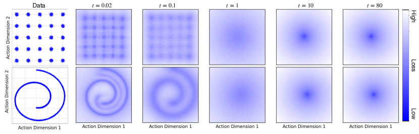
Figure 1: Diffusion trust region loss. The first column shows how the training behavior dataset looks. Columns 2-6 display the diffusion trust region loss on different actions with varying magnitudes of Gaussian noise. We can observe that the trust regions captured by the diffusion model at a given $t$ are consistent with the high-density regions of the noisy data at that specific $t$. For example, when $t$ is small, the diffusion loss is minimal where the true action lies, and high in all other locations.

2.4 Diffusion Trusted Q-Learning

We motivate our final algorithm from DQL (Wang et al., 2022a), which utilizes a diffusion model as an expressive policy to facilitate accurate policy regularization, ensuring that exploration remains within a safe region. Q-learning is implemented by maximizing the Q-value function at actions sampled from the diffusion policy. However, sampling actions from diffusion models can be time-consuming, and computing gradients of the Q-value function while backpropagating through all diffusion timesteps may result in a vanishing gradient problem, especially when the number of timesteps is substantial.

Building on this, we introduce a dual-policy approach, Diffusion Trusted Q-Learning (DTQL): a diffusion policy for pure behavior cloning and a one-step policy for actual depolyment. We bridge the two policies through our newly introduced diffusion trust region loss, detailed in Section 2.3. The diffusion policy ensures that behavior cloning remains expressive, while the trust region loss enables the one-step policy to explore freely and seek modes within the region designated by the diffusion policy. The trust region loss is optimized efficiently through each diffusion timestep without requiring the inference of the diffusion policy. DTQL not only maintains an expressive exploration region but also facilitates efficient optimization. We further discuss the mode-seeking behavior of the diffusion trust region loss in Section 3. Next, we delve into the specifics of our algorithm.

Policy Learning.

Diffusion inference is not required during training or evaluation in our algorithm; therefore, we utilize an unlimited number of timesteps and construct the diffusion policy $\mu_{\phi}$ in a continuous-time setting, based on the schedule outlined in EDM (Karras et al., 2022). Further details are provided in Section 4.3. The diffusion policy $\mu_{\phi}$ can be efficiently optimized by minimizing ${\mathcal{L}}(\phi)$ as described in Equation 2. Furthermore, we can instantiate one typical one-step policy $\pi_{\theta}({\bm{a}}|\bm{s})$ in two cases, Gaussian $\pi_{\theta}({\bm{a}}|\bm{s})={\mathcal{N}}(\mu_{\theta}({\bm{s}}),\sigma_{\theta}({\bm{s}}))$ or Implicit ${\bm{a}}_{\theta}=\pi_{\theta}({\bm{s}},\bm{\varepsilon}),\bm{\varepsilon}\sim{\mathcal{N}}(0,{\bm{I}})$. Then, we optimize $\pi_{\theta}$ by minimizing the introduced diffusion trust region loss and typical Q-value function maximization, as follows.

$$\mathcal{L}_{\pi}(\theta)=\alpha\cdot\mathcal{L}_{\text{TR}}(\theta)-\mathbb{E}_{\bm{s}\sim\mathcal{D},\bm{a}_{\theta}\sim\pi_{\theta}(\bm{a}|\bm{s})}[Q_{\eta}(\bm{s},\bm{a}_{\theta})],$$ (5)

where $\mathcal{L}_{\text{TR}}(\theta)$ serves primarily as a behavior-regularization term, and maximizing the Q-value function enables the model to preferentially sample actions associated with higher values. Here we use the double Q-learning trick (Hasselt, 2010) where $Q_{\eta}(\bm{s},\bm{a}_{\theta})=\min(Q_{\eta_{1}}(\bm{s},\bm{a}_{\theta}),Q_{\eta_{2}}(\bm{s},\bm{a}_{\theta}))$. If Gaussian policy is employed, it necessitates the introduction of an entropy term $-\mathbb{E}_{\bm{s},\bm{a}\sim\mathcal{D}}[\log\pi_{\theta}(\bm{a}|\bm{s})]$ to maintain an exploratory nature during training. This aspect is particularly crucial for diverse and sparse reward RL tasks. The empirical results of the entropy term will be discussed in Section 4.4.

Q-Learning.

We utilize Implicit Q-Learning (IQL) to train a Q function by maintaining two Q-functions $(Q_{\eta_{1}},Q_{\eta_{2}})$ and one value function $V_{\psi}$, following the methodology outlined in IQL (Kostrikov et al., 2021).

The loss function for the value function $V_{\psi}$ is defined as:

$${\mathcal{L}}_{V}(\psi)=\mathbb{E}_{({\bm{s}},{\bm{a}}\sim{\mathcal{D}})}\left[L_{2}^{\tau}\left(\min(Q_{{\eta}_{1}^{\prime}}({\bm{s}},{\bm{a}}),Q_{{\eta}_{2}^{\prime}}({\bm{s}},{\bm{a}}))-V_{\psi}({\bm{s}})\right)\right],$$ (6)

where $\tau$ is a quantile in $[0,1]$, and $L_{2}^{\tau}(u)=|\tau-\bm{1}(u<0)|u^{2}$. When $\tau=0.5$, $L_{2}^{\tau}$ simplifies to the $L_{2}$ loss. When $\tau>0.5$, $L_{\psi}$ encourages the learning of the $\tau$ quantile values of $Q$.

The loss function for updating the Q-functions, $Q_{\eta_{i}}$, is given by:

$${\mathcal{L}}_{Q}(\eta_{i})=\mathbb{E}_{({\bm{s}},{\bm{a}},{\bm{s}}^{\prime}\sim{\mathcal{D}})}\left[||r({\bm{s}},{\bm{a}})+\gamma*V_{\psi}({\bm{s}}^{\prime})-Q_{\eta_{i}}({\bm{s}},{\bm{a}})||^{2}\right],$$ (7)

where $\gamma$ denotes the discount factor. This setup aims to minimize the error between the predicted Q-values and the target values derived from the value function $V_{\psi}$ and the rewards. We summarize our algorithm in Algorithm 1.

Algorithm 1 Diffusion Trusted Q-Llearning

  Initialize policy network $\pi_{\theta}$, $\mu_{\phi}$, critic networks $Q_{\eta_{1}}$ and $Q_{\eta_{2}}$, and target networks $Q_{\eta_{1}^{\prime}}$ and $Q_{\eta_{2}^{\prime}}$, value function $V_{\psi}$

  for each iteration do

     Sample transition mini-batch ${\mathcal{B}}=\left\{({\bm{s}}_{t},{\bm{a}}_{t},r_{t},{\bm{s}}_{t+1})\right\}\sim{\mathcal{D}}$ .

      1. Q-value function learning: Update $Q_{\eta_{1}}$, $Q_{\eta_{2}}$ and $V_{\psi}$ by ${\mathcal{L}}_{Q}$ and ${\mathcal{L}}_{V}$ (Eqs. 6 and 7).

      2. Diffusion Policy learning: Update $\mu_{\phi}$ by ${\mathcal{L}}(\phi)$ (Eq. 2).

      3. Diffusion Trust Region Policy learning: ${\bm{a}}_{\theta}\sim\pi_{\theta}({\bm{a}}|{\bm{s}})$, Update $\pi_{\theta}$ by ${\mathcal{L}}_{\pi}(\theta)$ (Eq. 5).

      4. Update target networks: $\eta_{i}^{\prime}=\rho\eta_{i}^{\prime}+(1-\rho)\eta_{i}\mbox{ for }i=\{1,2\}$.

  end for

3 Mode seeking behavior regularization comparison

Another approach to accelerate training and inference in diffusion-based policy learning involves utilizing distillation techniques. Methods such as SDS (Poole et al., 2022), VSD (Wang et al., 2024), Diff-Instruct (Luo et al., 2024), and DMD (Yin et al., 2023) illustrate this strategy. These papers share a common theme: using a trained diffusion model alongside another diffusion network to minimize the KL divergence between the two models. In our experimental setup, this strategy is employed for behavior regularization by

$$\mathcal{L}_{\text{KL}}(\theta)=D_{\text{KL}}[\pi_{\theta}(\cdot|\bm{s})||\mu_{\phi}(\cdot|\bm{s})]=\mathbb{E}_{\bm{\varepsilon}\sim\mathcal{N}(0,\bm{I}),\bm{s}\sim\mathcal{D},\pi_{\theta}({\bm{s}},\bm{\varepsilon})}\left[\log\frac{p_{\text{fake}}(\bm{a}_{\theta}|\bm{s})}{p_{\text{real}}(\bm{a}_{\theta}|\bm{s})}\right]$$ (8)

where $\pi_{\theta}({\bm{s}},\bm{\varepsilon})$ is instantiates as an one-step Implicit policy.

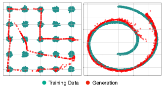
Figure 2: Green points represent the datasets we trained on. Red points are generated by $\pi_{\theta}$, trained using $\mathcal{L}_{\text{KL}}$. This demonstrates that the KL loss encourages the generation process to cover all modalities of the dataset.

As we do not have access to the log densities of the fake and true conditional distributions of actions, the loss itself cannot be calculated directly. However, we are able to compute the gradients. The gradient of $\log p_{\text{real}}(\bm{a}_{\theta}|\bm{s})$ can be estimated by the diffusion model $\mu_{\phi}(\cdot|\bm{s})$, and the gradient of $\log p_{\text{fake}}(\bm{a}_{\theta}|\bm{s})$ can also be estimated by a diffusion model trained from fake action data $\bm{a}_{\theta}$. For more details, please refer to Appendix D.

KL divergence is employed in this context with the goal of capturing all modalities of the data distribution. We evaluated this loss function using a 2D toy task to gain a deeper understanding of its capability to capture the complete modality of the dataset, as illustrated in Figure 2.

We further investigate the differences between our trust region loss and KL-based behavior distillation loss in the context of policy improvement. For $\mathcal{L}_{\text{TR}}$, as illustrated in Figure 1, the loss ensures that the generated action $\bm{a}_{\theta}$ lies within the in-sample datasets’ action manifold. With the gradient of the Q-function, it allows actions to freely move within the in-sample data manifold and gravitate towards high-reward regions.

Conversely, $\mathcal{L}_{\text{KL}}(\theta)$ aims to match the distribution of $\pi_{\theta}(\cdot|\bm{s})$ with $\mu_{\phi}(\cdot|\bm{s})$. This property is highly valued in image generation, where preserving diversity in the generated images is crucial. However, this is not necessarily advantageous in the RL community, where typically, a single highest-reward action is optimal for a given state. Moreover, maximizing the Q function can often lead to determinism by prioritizing the highest reward paths and overlooking alternative actions.

To visualize how these two different behavior losses work with policy improvement, we use 2D bandit scenarios. We designed a scenario shown in Figure 3; for additional settings, please refer to Appendix G.1. In the designed 25 Gaussian setting, all four corners have the same high reward. $\mathcal{L}_{\text{TR}}$ encourages the policy to randomly select one high reward mode without promoting covering all of them. In contrast, $\mathcal{L}_{\text{KL}}$ tries to cover all high-density and high-reward regions and, as a byproduct, introduces artifacts that appear as data connecting these high-density regions. This could partially be due to the smoothness constraint of neural networks. The same situation occurs in a Swiss roll dataset where the high reward region is the center of the data; $\mathcal{L}_{\text{TR}}$ adheres closely to the high reward region, while $\mathcal{L}_{\text{KL}}$ includes some suboptimal reward regions.

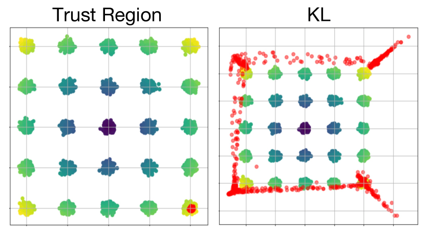
(a) 25 Guassian example with four corner have equally highest reward.

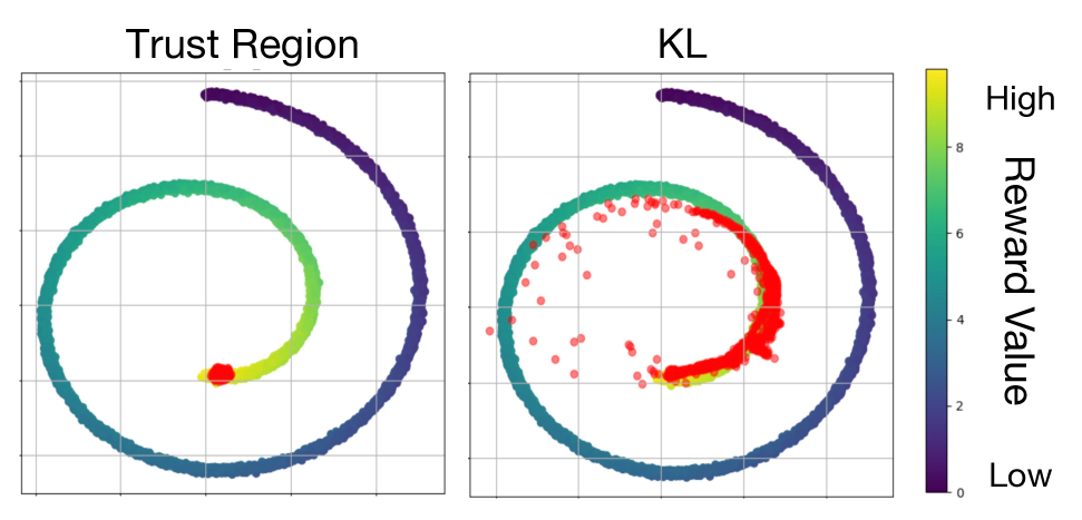
(b) Swiss roll example with center have highest reward.

Figure 3: We tested the differential impact of $\mathcal{L}_{\text{TR}}$ and $\mathcal{L}_{\text{KL}}$ on behavior regularization, using a trained Q-function for policy improvement. Red points represent actions generated from the one-step policy $\pi_{\theta}$.

In addition to testing on 2D bandit scenarios, we also evaluated the performance of two losses on the Mujoco Gym Medium task. Consistent with our previous findings, the behavior-regularization loss $\mathcal{L}_{\text{TR}}(\theta)$ consistently outperformed $\mathcal{L}_{\text{KL}}(\theta)$ in terms of achieving higher rewards. The results are presented in Table 5, and the training curves are depicted in Figure 7 in Appendix G.2.

Connection and Difference with SDS and SRPO

SDS was first proposed in DreamFusion (Poole et al., 2022) for 3D generation, using the gradient of the loss form (adopted in our setting):

$$\nabla_{\theta}\mathcal{L}_{\text{SDS}}=\mathbb{E}_{t,\bm{s},\bm{\varepsilon}}\left[w(t)(\varepsilon_{\phi}(\bm{z}_{t},t|\bm{s})-\bm{\varepsilon})\frac{\partial\bm{z}_{t}}{\partial\theta}\right]$$ (9)

where $\bm{z}_{t}=\alpha_{t}\bm{a}_{\theta}+\sigma_{t}\bm{\varepsilon}$ and $\varepsilon_{\phi}$ is the noise-prediction diffusion model. This loss is utilized by SRPO (Chen et al., 2023) in offline RL.

Considering the gradient of $\mathcal{L}_{\text{TR}}(\theta)$ in Equation 4, and acknowledging the equivalence between noise-prediction and data-prediction diffusion models with only a modification in the weight function $w(t)$, we can reformulate the loss in noise-prediction form by:

$$\mathcal{L}_{\text{TR}}(\theta) =\mathbb{E}_{t,\bm{s},\bm{\varepsilon}}[w^{\prime}(t)\|\varepsilon_{\phi}(\bm{z}_{t},t|\bm{s})-\bm{\varepsilon}\|_{2}^{2}]$$ (10)

$$\nabla_{\theta}\mathcal{L}_{\text{TR}}(\theta) =2\mathbb{E}_{t,\bm{s},\bm{\varepsilon}}\left[w^{\prime}(t)(\varepsilon_{\phi}(\bm{z}_{t},t|\bm{s})-\bm{\varepsilon})\frac{\partial\varepsilon_{\phi}(\bm{z}_{t},t|\bm{s})}{\partial\bm{z}_{t}}\frac{\partial\bm{z}_{t}}{\partial\theta}\right]$$ (11)

The primary distinction between the gradient of our method, as shown in Equation 11, and that of SDS/SRPO, detailed in Equation 9, lies in the inclusion of a Jacobian term, $\frac{\partial\epsilon_{\phi}(\bm{z}_{t},t|\bm{s})}{\partial\bm{z}_{t}}$. This Jacobian term, identified as the score gradient in SiD by Zhou et al. (2024), is notably absent from most theoretical discussions and was deliberately omitted in previous works, with DreamFusion (Poole et al., 2022) and SiD being the sole exceptions.

DreamFusion reported that the gradient depicted in Equation 11 fails to produce realistic 3D samples. Similarly, SiD observed its inadequacy in generating realistic images. These findings align with our Theorem 1, which demonstrates that this gradient primarily targets the mode and does not sufficiently account for diversity— an essential factor in both 3D and image generation.

In high-dimensional generative models, modes often differ significantly from typical image samples, as discussed by Nalisnick et al. (2018). DreamFusion observed that the gradient from Equation 9, which is based on a KL loss, effectively promotes diversity. However, while diversity is crucial in image and 3D generation, it is of lesser importance in offline RL. Consequently, SRPO’s use of the SDS gradient, which is tailored for diverse generation, may result in suboptimal performance compared to our diffusion trust region loss. This assertion is supported by empirical results on the D4RL datasets, as discussed in Section 4.1.

4 Experiments

In this section, we evaluate our method using the popular D4RL benchmark (Fu et al., 2020). We further compare our training and inference efficiency against other baseline methods. Additionally, an ablation study on the entropy term and one-step policy choice is presented. Details regarding the training of the diffusion model and its structural components are also discussed.

Hyperparameters

In D4RL benchmarks, for all Antmaze tasks, we incorporate an entropy term, while for other tasks, this term is omitted. Additionally, we adjust the parameter $\alpha$ for different tasks. Details on hyperparameters and implementation are provided in Appendices E and F.

4.1 D4RL Performance

In Table 1, we evaluate the D4RL performance of our method against other offline algorithms. Our selected benchmarks include conventional methods such as TD3+BC (Fujimoto and Gu, 2021) and IQL (Kostrikov et al., 2021), along with newer diffusion-based models like Diffusion QL (DQL) (Wang et al., 2022a), IDQL (Hansen-Estruch et al., 2023), and SRPO (Chen et al., 2023).

Table 1: The performance of Our methods and SOTA baselines on D4RL Gym, AntMaze, Adroit, and Kitchen tasks. Results for our methods correspond to the mean and standard errors of normalized scores over 50 random rollouts (5 independently trained models and 10 trajectories per model) for Gym tasks, which generally exhibit low variance in performance, and over 500 random rollouts (5 independently trained models and 100 trajectories per model) for the other tasks. Our method outperforms all prior methods by a clear margin on most of domains. The normalized scores is recorded by the end of training phase. Numbers within 5 % of the maximum in every individual task are highlighted.

Gym	BC	Onestep RL	TD3+BC	DT	CQL	IQL	DQL	IDQL	SRPO	Ours
halfcheetah-medium-v2	42.6	48.4	48.3	42.6	44.0	47.4	51.1	51.0	60.4	57.9 $\pm$ 0.13
hopper-medium-v2	52.9	59.6	59.3	67.6	58.5	66.3	90.5	65.4	95.5	99.6$\pm$0.87
walker2d-medium-v2	75.6	81.8	83.7	74.0	72.5	78.3	87.0	82.5	84.4	89.4$\pm$0.13
halfcheetah-medium-replay-v2	36.3	38.1	44.6	36.0	45.2	44.2	47.8	45.9	51.4	50.9$\pm$0.11
hopper-medium-replay-v2	18.1	97.5	60.9	82.7	95.0	94.7	101.3	92.1	101.2	100.0$\pm$0.13
walker2d-medium-replay-v2	26.0	49.5	81.8	66.6	77.2	73.9	95.5	85.1	84.6	88.5$\pm$ 2.16
halfcheetah-medium-expert-v2	55.2	93.4	90.7	86.8	91.6	86.7	96.8	95.9	92.2	92.7 $\pm$ 0.2
hopper-medium-expert-v2	52.5	103.3	98.0	107.6	105.8	91.5	111.1	108.6	100.1	109.3 $\pm$ 1.49
walker2d-medium-expert-v2	101.9	113.0	110.1	107.1	109.4	109.6	110.1	112.7	114.0	110 $\pm$ 0.07
Gym Average	51.9	76.1	75.3	74.7	77.6	77.0	88.0	82.1	87.1	88.7
Antmaze	BC	Onestep RL	TD3+BC	DT	CQL	IQL	DQL	IDQL	SRPO	Ours
antmaze-umaze-v0	54.6	64.3	78.6	59.2	74.0	87.5	93.4	94.0	90.8	94.8$\pm$1.00
antmaze-umaze-diverse-v0	45.6	60.7	71.4	53.0	84.0	62.2	66.2	80.2	59.0	78.8$\pm$1.83
antmaze-medium-play-v0	0.0	10.6	0.0	0.0	61.2	71.2	76.6	84.5	73.0	79.6 $\pm$ 1.8
antmaze-medium-diverse-v0	0.0	3.0	0.2	0.0	53.7	70.0	78.6	84.8	65.2	82.2 $\pm$ 1.71
antmaze-large-play-v0	0.0	0.0	0.0	0.0	15.8	39.6	46.4	63.5	38.8	52.0$\pm$ 2.23
antmaze-large-diverse-v0	0.0	0.0	0.0	0.0	14.9	47.5	56.6	67.9	33.8	54.0 $\pm$ 2.23
Antmaze Average	16.7	20.9	27.3	18.7	50.6	63.0	69.6	79.1	30.1	73.6
Adroit Tasks	BC	BCQ	BEAR	BRAC-p	BRAC-v	REM	CQL	IQL	DQL	Ours
pen-human-v1	25.8	68.9	-1.0	8.1	0.6	5.4	35.2	71.5	72.8	64.1$\pm$2.97
pen-cloned-v1	38.3	44.0	26.5	1.6	-2.5	-1.0	27.2	37.3	57.3	81.3$\pm$ 3.04
Adroit Average	32.1	56.5	12.8	4.9	-1.0	2.2	31.2	54.4	65.1	72.7
Kitchen Tasks	BC	BCQ	BEAR	BRAC-p	BRAC-v	AWR	CQL	IQL	DQL	Ours
kitchen-complete-v0	33.8	8.1	0.0	0.0	0.0	0.0	43.8	62.5	84.0	80.8$\pm$1.06
kitchen-partial-v0	33.8	18.9	13.1	0.0	0.0	15.4	49.8	46.3	60.5	74.4$\pm$0.25
kitchen-mixed-v0	47.5	8.1	47.2	0.0	0.0	10.6	51.0	51.0	62.6	60.2$\pm$0.59
Kitchen Average	38.4	11.7	20.1	0.0	0.0	8.7	48.2	53.3	69.0	71.8

In the D4RL datasets, our method (DTQL) outperformed all conventional and other diffusion-based offline RL methods, including DQL and SRPO, across all tasks. Moreover, it is 10 times more efficient in inference than DQL and IDQL; and 5 times more efficient in total training wall time compared with IDQL (see Section 4.2).

Remark 3.

We would like to highlight that the SRPO method (Chen et al., 2023) reported results on Antmaze using the “-v2” version, which differs from the “-v0” version employed by prior methods such as DQL (Wang et al., 2022a) and IDQL (Hansen-Estruch et al., 2023), to which it was compared. This version discrepancy, not explicitly stated in their paper, is evident upon inspection of SRPO’s official codebase . The variation between the -v2” and -v0” datasets significantly impacts algorithm performance. To ensure a fair comparison, we utilize the “-v0” environments consistent with established baselines. We employed the official SRPO code on Antemze-v0 and maintained identical hyperparameters used for Antmaze-v2. Additionally, we conducted experiments with our algorithm on the Antmaze-v2 environment using the same hyperparameters as in the Antmaze-v0 setup but extended the training epochs, as detailed in Table 6 in Appendix G.

4.2 Computational Efficiency

We further examine the training and inference performance relative to other diffusion-based offline RL methods. An overview of this performance, using antmaze-umaze-v0 as a benchmark, is presented in Table 2. Our method requires less training time per epoch than DQL and SRPO, yet more than IDQL. However, while IDQL necessitates 3000 epochs, DTQL operates efficiently with only 500 epochs, considerably reducing the overall training duration.

As depicted in Figure 4, the extended training time per epoch for our method results from the requirement to train an additional one-step policy, a step not needed by IDQL. Although SRPO also incorporates a one-step policy, our method achieves greater efficiency in training the diffusion policy. Unlike SRPO, which requires several ResNet blocks for effective performance, our approach utilizes only a 4-layer MLP, further curtailing the training time. Additional details on total training wall time are provided in Appendix G.4.

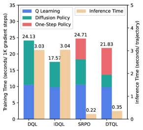
Figure 4: Training time required for different algorithms in D4RL antmaze-umaze-v0 tasks. All experiments are conducted with the same PyTorch backend and the same computing hardware setup.

For inference time, our method performs comparably to SRPO, as both utilize a one-step policy. However, our method achieves a tenfold increase in inference speed over DQL and IDQL, which require 5-step iterative denoising to generate actions. All experiments were conducted on a server equipped with 8 RTX-A5000 GPUs.

Table 2: Training and Inference time required for different algorithms in D4RL antmaze-umaze-v0 tasks. Every single experiment is conducted with the same PyTorch backend and run on 1 RTX-A5000 GPU.

antmaze-umaze-v0	DQL	IDQL	SRPO	Ours
Training time (s per 1k steps)	24.13	17.57	24.71	21.83
Inference time (s per trajectory)	3.03	3.04	0.22	0.35
Training epochs	1000	3000	1000	500
Total training time (hours)	6.70	14.64	9.42	3.33

Remark 4.

For total training time, SRPO trains 1000 epochs for the one-step policy while training 1500 epochs for the diffusion policy and Q function. DTQL requires 50 epochs of pretraining. Implement details are in Appendix E.

4.3 Diffusion Training Schedule

For training the diffusion policy as described in Equation 2 and the diffusion trust region loss in Equation 4, we utilize the diffusion weight and noise schedule outlined in EDM (Karras et al., 2022). Although EDM does not satisfy the ELBO condition stipulated in Equation 3—a fact established in (Kingma and Gao, 2024)—we adopted it due to its demonstrated enhancements in perceptual generation quality, as evidenced by metrics such as the Fréchet Inception Distance (FID) and Inception Score in the field of image generation. Kingma and Gao (2024) also attempted to modify the EDM weight schedule to be monotonically increasing, but this did not lead to better FID. Thus, we retain EDM as our continuous training schedule. For completeness, the details of the EDM schedule are discussed in Appendix C.

4.4 Ablation Studies

One-step Policy Choice

We chose to use a Gaussian policy for all our experiments instead of an implicit or deterministic policy because the Gaussian policy is flexible and provides a convenient way to control entropy when needed. When there is no need to maintain entropy, the Gaussian policy quickly degenerates to a deterministic policy, where the variance approaches zero, as indicated in Figures 5(b) and 5(d).

Entropy Term

As mentioned in Section 2.4, we incorporate an entropy term $-\mathbb{E}_{\bm{s},\bm{a}\sim\mathcal{D}}[\log\pi(\bm{a}|\bm{s})]$ into the loss function in Equation 5 to maintain exploration during training when using a Gaussian policy. We conducted an ablation study to assess its impact on the final rewards and the entropy of the Gaussian policy, taking antmaze-umaze-v0 and antmaze-large-diverse-v0 as examples. As observed in Figure 5, for the less complex task antmaze-umaze-v0, adding the entropy term does not significantly enhance the final score but does stabilize the training process (see Figure 5(a)). However, for more complex tasks like antmaze-large-diverse-v0, the addition of the entropy term markedly increases the final score. We attribute this improvement to the ability of the entropy term to maintain high entropy during training, thus preserving exploration capabilities, as shown in Figures 5(b) and 5(d).

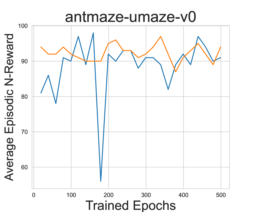
(a) Reward Curve

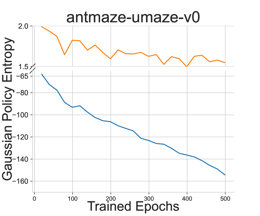
(b) Entropy Curve

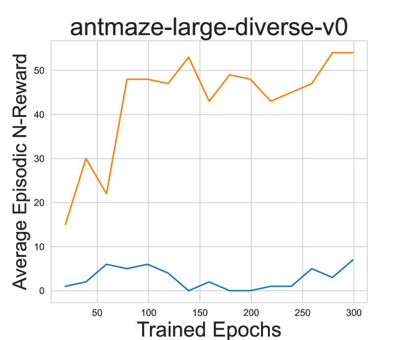
(c) Reward Curve

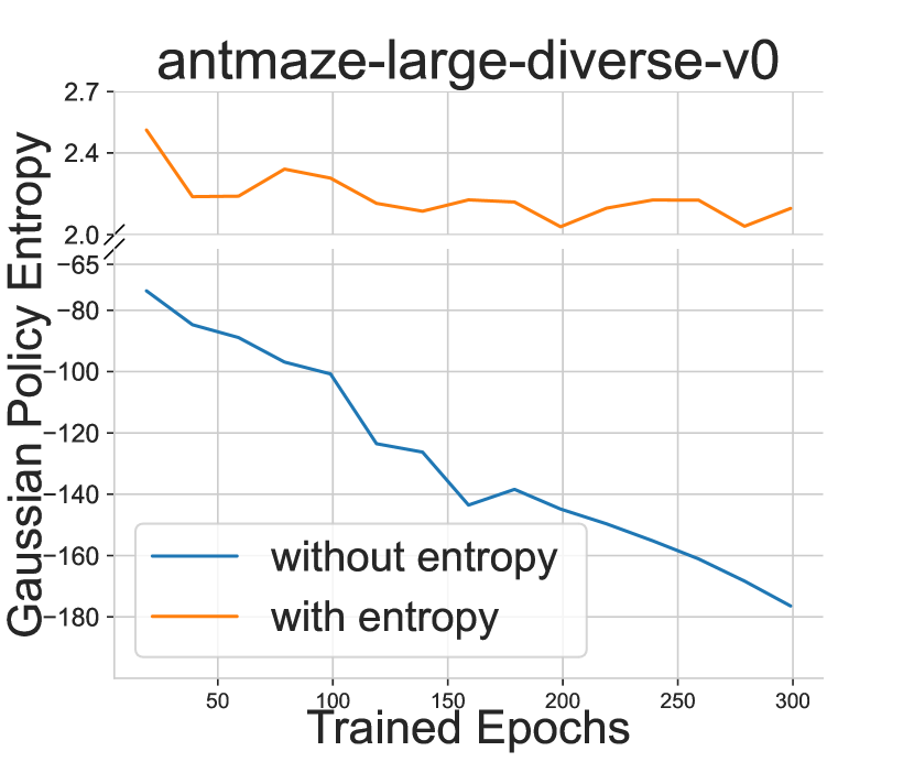
(d) Entropy Curve

Figure 5: Rewards and Gaussian policy entropy during training are recorded and illustrated in the figures. The blue line represents training without the addition of an entropy term, while the orange line indicates training with the entropy term included.

5 Conclusion and Limitation

In this work, we present DTQL, which comprises a diffusion policy for pure behavior cloning and a practical one-step policy. The diffusion policy maintains expressiveness, while the diffusion trust region loss introduced in this paper directs the one-step policy to explore freely and seek modes within the safe region defined by the diffusion policy. This training pipeline eliminates the need for iterative denoising sampling during both training and inference, making it remarkably computationally efficient. Moreover, DTQL achieves state-of-the-art performance across the majority of tasks in the D4RL benchmark. Some limitations of DTQL include the potential for improvement in its benchmark performance. Additionally, some design aspects of the one-step policy could benefit from further investigation. Currently, our experiments are primarily conducted in an offline setting. It would be interesting to explore how this method can be extended to an online setting or adapted to handle more complex inputs, such as images. Moreover, instead of performing point estimation of reward, it would be worthwhile to estimate the distribution of rewards, as suggested by (Yue et al., 2020), (Bellemare et al., 2017), and (Barth-Maron et al., 2018).

Diffusion Policies creating a Trust Region for
Offline Reinforcement Learning: Appendix

Appendix A Broader Impacts

Reinforcement learning influences various fields, including healthcare, finance, autonomous systems, education, and sustainability. However, it also raises ethical concerns, job displacement issues, and decision-making biases, necessitating careful mitigation strategies.

Appendix B Related Work

Expressive Generative Models for Behavior Cloning

Behavior cloning refers to the task of learning the behavior policy that was used to collect static datasets. Generative models are often employed for behavior cloning due to their expressive power. For instance, EMaQ [Ghasemipour et al., 2021] uses an auto-regressive model for behavior cloning. BCQ [Fujimoto et al., 2019] utilizes a Conditional Variational Autoencoder (VAE), while Florence et al. [2022] employ energy-based models. GAN-Joint [Yang et al., 2022] leverages GANs, and several studies [Wang et al., 2022a, Janner et al., 2022, Pearce et al., 2023] utilize diffusion models for behavior cloning. Diffusion models have demonstrated strong performance due to their ability to capture multimodal distributions. However, they may suffer from increased training and inference times because of the iterative denoising process required for sampling.

Efficiency Improvement in Diffusion-Based RL Methods.

Several studies aim to accelerate the training of diffusion models in offline RL settings. One approach involves using specialized diffusion ODE solvers, such as the DDIM solver [Song et al., 2020a] or the DPM-solver [Lu et al., 2022], to speed up iterative sampling. Another strategy is to avoid iterative denoising during training or inference. EDP [Kang et al., 2024] and IDQL [Hansen-Estruch et al., 2023] both focus on avoiding iterative sampling during training. EDP adopts an approximate diffusion sampling scheme to minimize the required sampling steps, although it still requires iterative denoising during inference. IDQL accelerates the training process by only training a behavior cloning policy without denoising sampling. However, it requires iterative sampling during inference by selecting from a batch of candidate generated actions. SRPO [Chen et al., 2023] employs score distillation methods to avoid iterative denoising in both training and inference.

Distillation Methods.

Distillation methods for diffusion models have been proposed to enable one-step generation of images or 3D objects. Examples of such methods include SDS [Poole et al., 2022], VSD [Wang et al., 2024], Diff Instruct [Luo et al., 2024], and DMD [Yin et al., 2023]. The core idea of these methods is to minimize the KL divergence between a pre-trained diffusion model and a target one-step generation model. SiD [Zhou et al., 2024] uses a different divergence metric but shares the same goal of mimicking the distribution learned by a pre-trained diffusion model. The distillation strategy can also be applied in the offline RL field to accelerate training and inference. However, directly adopting these methods may result in suboptimal performance.

Appendix C Diffusion Schedule

This diffusion training schedule is same for training the behavior-cloning policy in Equation 2 and the diffusion trust region loss in Equation 4.

Noise Schedule

We illustrate the EDM diffusion training schedule in our setting. First, we need to define some prespecified parameters: $\sigma_{\text{data}}=0.5$, $\sigma_{\text{min}}=0.002$, $\sigma_{\text{max}}=80$. The noise schedule is defined by $\bm{a}_{t}=\alpha_{t}\bm{a}+\sigma_{t}\bm{\varepsilon}$, where $\bm{\varepsilon}\sim\mathcal{N}(0,\bm{I})$. We set $\alpha_{t}=1$ and $\sigma_{t}=t$. The variable $\log(t)$ follows a logistic distribution with location parameter $\log\sigma_{\text{data}}$ and scale parameter $0.5$. The original EDM paper samples $\log(t)$ from $\mathcal{N}(-1.2,1.2^{2})$, but this difference does not significantly affect our algorithm.

Denoiser

The denoiser $\mu_{\phi}$ is defined as:

$$\mu_{\phi}(\bm{a}_{t},t|\bm{s})=c_{\text{skip}}(\sigma)\bm{a}_{t}+c_{\text{out}}(\sigma)F_{\phi}(c_{\text{in}}(\sigma)\bm{a}_{t},c_{\text{noise}}(\sigma)|\bm{s}),$$

where $\sigma=\sigma_{t}=t$ and $F_{\phi}$ represents the raw neural network layer. We also define:

$$c_{\text{skip}}(\sigma) =\frac{\sigma_{\text{data}}^{2}}{\sigma^{2}+\sigma_{\text{data}}^{2}},~{}~{}c_{\text{out}}(\sigma)=\frac{\sigma\cdot\sigma_{\text{data}}}{\sqrt{\sigma^{2}+\sigma_{\text{data}}^{2}}},$$

$$c_{\text{in}}(\sigma) =\frac{1}{\sigma^{2}+\sigma_{\text{data}}^{2}},~{}~{}c_{\text{noise}}(\sigma)=\frac{1}{4}\log(\sigma).$$

Weight Schedule

The final loss is given by:

$$\mathbb{E}_{\sigma,\bm{a},\bm{s},\bm{\varepsilon}}\left[\lambda(\sigma)c_{\text{out}}^{2}(\sigma)\left\|F_{\phi}(c_{\text{in}}(\sigma)\cdot(\bm{a}+\bm{\varepsilon}),c_{\text{noise}}(\sigma)|\bm{s})-\frac{1}{c_{\text{out}}(\sigma)}\left(\bm{a}-c_{\text{skip}}(\sigma)\cdot(\bm{a}+\bm{\varepsilon})\right)\right\|_{2}^{2}\right],$$

where $\lambda(\sigma)=\frac{1}{c_{\text{out}}^{2}(\sigma)}$.

Appendix D Details in KL Behavior Regularization

Here we introduce how we implement KL divergence regularization. The idea is similar to previous KL-based distillation methods [Wang et al., 2024, Luo et al., 2024, Yin et al., 2023], but adapted to our setting. Our loss function is defined as:

$$\mathcal{L}_{\text{KL}}(\theta)=D_{\text{KL}}[\pi_{\theta}(\cdot|\bm{s})||\mu_{\phi}(\cdot|\bm{s})]=\mathbb{E}_{\bm{\varepsilon}\sim\mathcal{N}(0,\bm{I}),\bm{s}\sim\mathcal{D},\pi_{\theta}(\bm{s},\bm{\varepsilon})}\left[\log\frac{p_{\text{fake}}(\bm{a}_{\theta}|\bm{s})}{p_{\text{real}}(\bm{a}_{\theta}|\bm{s})}\right]$$ (12)

The gradient of $\mathcal{L}_{\text{KL}}(\theta)$ is given by:

$$\nabla_{\theta}\mathcal{L}_{\text{KL}}(\theta)=\mathbb{E}_{\bm{\varepsilon},\bm{s},\bm{a}_{\theta}=\pi_{\theta}(\bm{s},\bm{\varepsilon})}\left[\left(s_{\text{fake}}(\bm{a}_{\theta}|\bm{s})-s_{\text{real}}(\bm{a}_{\theta}|\bm{s})\right)\nabla_{\theta}\pi_{\theta}\right]$$

where $s_{\text{real}}(\bm{a}_{\theta}|\bm{s})=\nabla_{\bm{a}_{\theta}}\log p_{\text{real}}(\bm{a}_{\theta}|\bm{s})$ and $s_{\text{fake}}(\bm{a}_{\theta}|\bm{s})=\nabla_{\bm{a}_{t}heta}\log p_{\text{fake}}(\bm{a}_{\theta}|\bm{s})$. By using the Score-ODE given in [Song et al., 2020b], we can estimate $s_{\text{real}}(\bm{a}_{\theta}|\bm{s})$ and $s_{\text{fake}}(\bm{a}_{\theta}|\bm{s})$ with a diffusion model. Let $\bm{a}_{\theta,t}=\alpha_{t}\bm{a}_{\theta}+\sigma_{t}\bm{\varepsilon}$, the real score can be estimated by:

$$s_{\text{real}}(\bm{a}_{\theta,t},t|\bm{s})=-\frac{\bm{a}_{\theta,t}-\alpha_{t}\mu_{\phi}(\bm{a}_{\theta,t},t|\bm{s})}{\sigma_{t}^{2}}$$

where $\mu_{\phi}$ is the pre-trained diffusion behavior cloning model that learns the true data distribution.

Similarly, we can estimate the fake score by:

$$s_{\text{fake}}(\bm{a}_{\theta,t},t|\bm{s})=-\frac{\bm{a}_{\theta,t}-\alpha_{t}\mu_{\xi}(\bm{a}_{\theta,t},t|\bm{s})}{\sigma_{t}^{2}}$$

where $\mu_{\xi}$ is trained using fake data:

$$\mathcal{L}(\xi)=\|\mu_{\xi}(\bm{a}_{\theta,t},t|\bm{s})-\bm{a}_{\theta}\|_{2}^{2}$$

which is trained with generated fake action data.

Thus, the gradient of $\mathcal{L}_{\text{KL}}(\theta)$ can be expressed as:

$$\nabla_{\theta}\mathcal{L}_{\text{KL}}(\theta)=\mathbb{E}_{\bm{\varepsilon},\bm{s},\bm{a}_{\theta},\bm{a}_{\theta,t}}\left[w_{t}\alpha_{t}\left(s_{\text{fake}}(\bm{a}_{\theta,t},t|\bm{s})-s_{\text{real}}(\bm{a}_{\theta,t},t|\bm{s})\right)\nabla_{\theta}\pi_{\theta}\right]$$

where $w_{t}=\frac{\sigma_{t}^{2}}{\alpha_{t}}\frac{A}{\|\mu_{\phi}(\bm{a}_{\theta,t},t)-\bm{a}_{\theta}\|_{1}}$ and $A$ is the dimension of the action space.

The algorithm for KL regularization is shown below:

Algorithm 2 KL Regularization

  Initialize policy network $\pi_{\theta}$, $\mu_{\phi}$, $\mu_{\xi}$

  for each iteration do

     Sample transition mini-batch $\mathcal{B}=\{(\bm{s}_{t},\bm{a}_{t},r_{t},\bm{s}_{t+1})\}\sim\mathcal{D}$

     Diffusion Policy Learning: Update $\mu_{\phi}$ by $\mathcal{L}(\phi)$

  end for

  Initialize policy and fake score network: $\theta\leftarrow\phi$, $\xi\leftarrow\phi$

  for each iteration do

     Sample transition mini-batch $\mathcal{B}=\{(\bm{s}_{t},\bm{a}_{t},r_{t},\bm{s}_{t+1})\}\sim\mathcal{D}$, generate $\bm{a}_{\theta}$

     Random timestep and add noise: Choose $t$, $\bm{a}_{\theta_{t}}=\alpha_{t}\bm{a}_{\theta}+\sigma_{t}\varepsilon$

     with_no_grad():

         $pred\_fake\_action=\mu_{\xi}(\bm{a}_{\theta_{t}},t|\bm{s})$

         $pred\_real\_action=\mu_{\phi}(\bm{a}_{\theta_{t}},t|\bm{s})$

     $weighting\_factor=\text{abs}(\bm{a}_{\theta}-pred\_real\_action).\text{mean}(\text{keepdim=True})$

     $grad=\frac{pred\_fake\_action-pred\_real\_action}{weighting\_factor}$

     $loss=0.5\times\text{mse\_loss}(\bm{a}_{\theta},\text{stopgrad}(\bm{a}_{\theta}-grad))$

     Update $\pi_{\theta}$ by $loss$

     Diffusion Fake Policy Learning: Update $\mu_{\xi}$ by $\mathcal{L}(\xi)$

  end for

Appendix E Implementation Details

Diffusion Policy

We build our policy as an MLP-based conditional diffusion model. The model itself is an action prediction model. We model $\mu_{\phi}$ and $\mu_{\xi}$ as 4-layer MLPs with Mish activations, using 256 hidden units for all networks. The input to $\mu_{\phi}$ and $\mu_{\xi}$ is the concatenation of the noisy action vector, the current state vector, and the sinusoidal positional embedding of timestep $t$. The output of $\mu_{\phi}$ and $\mu_{\xi}$ is the predicted action at diffusion timestep $t$.

Q and V Networks

We build two Q networks and a V network with the same MLP setting as our diffusion policy. Each network comprises 4-layer MLPs with Mish activations and 256 hidden units.

One-Step Policy

We build a Gaussian policy using 3-layer MLPs with ReLU activations, utilizing 256 hidden units. After sampling an action, we apply a tanh activation to ensure the action lies between $[-1,1]$. If an implicit policy is instantiated, its structure is the same as that of the diffusion policy.

Pretrain

In our implementation, we pretrain the diffusion policy $\mu_{\phi}$ and the Q function $Q_{\eta}$ for 50 epochs to ensure they can better guide $\pi_{\theta}$. Then, $\mu_{\phi}$, $Q_{\eta}$, and $\pi_{\theta}$ are concurrently trained for the epochs specified in Table 4. We found that introducing a pretrain schedule does not significantly influence the final performance. Our ablation study on the Gym Medium Task revealed that while pretraining yields slightly better results, the final rewards are largely similar. Therefore, we maintain a 50-epoch pretrain for all our tasks. The results are shown in Table 3.

Table 3: The performance with and without pretraining on D4RL Gym tasks.

Environment	Pretrain	No Pretrain
halfcheetah-medium-v2	57.9	57.5
hopper-medium-v2	99.6	87.6
walker2d-medium-v2	89.4	88.7

Appendix F Hyperparamaters

Table 4: Hyperparameters for D4RL benchmarks. One epoch represents 1k steps, and the optimizer used is Adam.

Gym	$\bm{\alpha}$	$\bm{\tau}$	Entropy Term	Pretrain Epochs	Training Epochs	Learning Rate	Lr decay
halfcheetah-medium-v2	1	0.7	False	50	1000	$3\times 10^{-4}$	False
halfcheetah-medium-replay-v2	5	0.7	False	50	1000	$3\times 10^{-4}$	False
halfcheetah-medium-expert-v2	50	0.7	False	50	1000	$3\times 10^{-4}$	False
hopper-medium-v2	5	0.7	False	50	1000	$1\times 10^{-4}$	True
hopper-medium-replay-v2	5	0.7	False	50	1000	$3\times 10^{-4}$	False
hopper-medium-expert-v2	20	0.7	False	50	1000	$3\times 10^{-4}$	False
walker2d-medium-v2	5	0.7	False	50	1000	$3\times 10^{-4}$	True
walker2d-medium-replay-v2	5	0.7	False	50	1000	$3\times 10^{-4}$	True
walker2d-medium-expert-v2	5	0.7	False	50	1000	$3\times 10^{-4}$	True
antmaze-umaze-v0	1	0.9	True	50	500	$3\times 10^{-4}$	False
antmaze-umaze-diverse-v0	1	0.9	True	50	500	$3\times 10^{-5}$	True
antmaze-medium-play-v0	1	0.9	True	50	400	$3\times 10^{-4}$	False
antmaze-medium-diverse-v0	1	0.9	True	50	400	$3\times 10^{-4}$	False
antmaze-large-play-v0	1	0.9	True	50	350	$3\times 10^{-4}$	False
antmaze-large-diverse-v0	0.5	0.9	True	50	300	$3\times 10^{-4}$	False
antmaze-umaze-v2	1	0.9	True	50	500	$3\times 10^{-4}$	False
antmaze-umaze-diverse-v2	1	0.9	True	50	500	$3\times 10^{-5}$	True
antmaze-medium-play-v2	1	0.9	True	50	500	$3\times 10^{-4}$	False
antmaze-medium-diverse-v2	1	0.9	True	50	500	$3\times 10^{-4}$	False
antmaze-large-play-v2	1	0.9	True	50	500	$3\times 10^{-4}$	False
antmaze-large-diverse-v2	0.5	0.9	True	50	500	$3\times 10^{-4}$	False
pen-human-v1	1500	0.9	False	50	300	$3\times 10^{-5}$	True
pen-cloned-v1	1500	0.7	False	50	200	$1\times 10^{-5}$	False
kitchen-complete-v0	200	0.7	False	50	500	$1\times 10^{-4}$	True
kitchen-partial-v0	100	0.7	False	50	1000	$1\times 10^{-4}$	True
kitchen-mixed-v0	200	0.7	False	50	500	$3\times 10^{-4}$	True

Appendix G Additional Experiments

G.1 Complete 2D Toy Experiments

We also conducted some 2D bandit experiments with different reward scenarios. In Figure 6, red points are generated by the one-step policy $\pi_{\theta}$.

In the first column, where the four corners have the same high reward, $\mathcal{L}_{\text{KL}}$ tends to encourage exploration of all these high-reward regions, resulting in some suboptimal reward actions. In contrast, $\mathcal{L}_{\text{TR}}$ generates actions that randomly select one of the high-reward regions, thereby avoiding suboptimal actions. The same situation occurs in the fourth and fifth columns of Figure 6, where $\mathcal{L}_{\text{KL}}$ covers some suboptimal regions while $\mathcal{L}_{\text{TR}}$ adheres closely to the highest reward regions.

However, when the data have only one mode with the highest reward, such as in the second and third columns of Figure 6, both $\mathcal{L}_{\text{KL}}$ and $\mathcal{L}_{\text{TR}}$ guide the policy to generate high-reward actions.

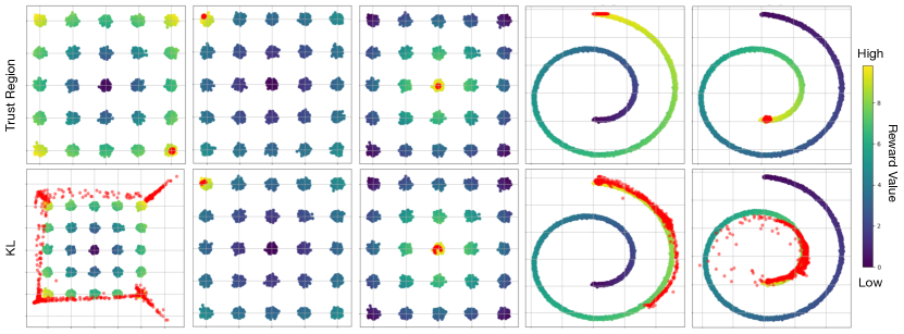
Figure 6: 2D Bandit toy examples, where the behavior regularization is conducted by $\mathcal{L}_{\text{TR}}$ and $\mathcal{L}_{\text{KL}}$ in different behavior data and reward scenarios. The first row uses behavior regularization by $\mathcal{L}_{\text{TR}}$, and the second row uses $\mathcal{L}_{\text{KL}}$. Yellow indicates the highest reward, and dark blue indicates the lowest reward.

G.2 Comparison with KL behavior Regularization in Gym Tasks

In addition to testing on 2D bandit scenarios, we also evaluated the performance of two losses ${\mathcal{L}}_{\text{KL}}$ and ${\mathcal{L}}_{\text{TR}}$ on the Mujoco Gym Medium task. The behavior regularization loss $\mathcal{L}_{\text{TR}}(\theta)$ consistently outperformed $\mathcal{L}_{\text{KL}}(\theta)$ in terms of achieving higher rewards. The results are presented in Table 5, and the training curves are depicted in Figure 7.

Table 5: The performance of $\mathcal{L}_{\text{TR}}(\theta)$ and $\mathcal{L}_{\text{KL}}(\theta)$ on D4RL Gym tasks. Results correspond to the mean of normalized scores over 50 random rollouts (5 independently trained models and 10 trajectories per model).

Environment	$\mathcal{L}_{\text{TR}}(\theta)$	$\mathcal{L}_{\text{KL}}(\theta)$
halfcheetah-medium-v2	$\bm{57.9}$	24.1
hopper-medium-v2	$\bm{99.6}$	15.0
walker2d-medium-v2	$\bm{89.4}$	3.4

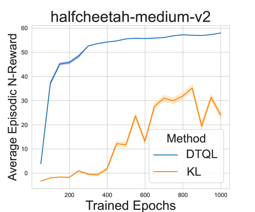
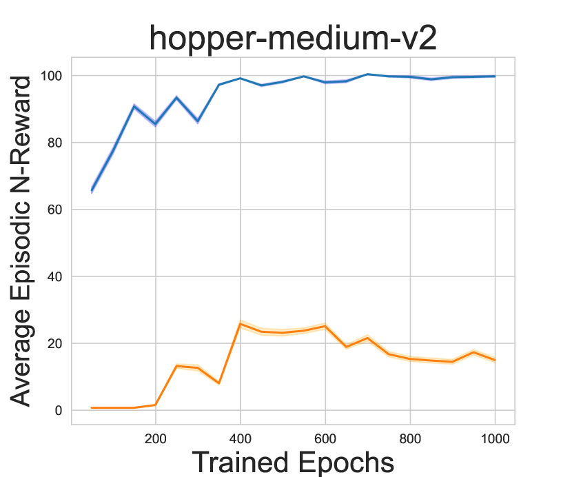
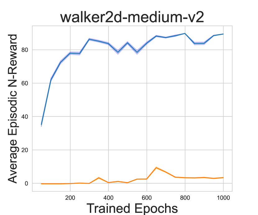
Figure 7: Training curves comparing policy learning with diffusion trust region loss and KL loss across three Gym medium tasks demonstrate that diffusion trust region regularization (DTQL) consistently outperforms KL-based behavior regularization in policy learning.

G.3 Comparison with SRPO on Antmaze-v2 Datasets

Since SRPO uses Antmaze-v2 for their D4RL benchmarks, we also conducted experiments on Antmaze-v2 using our algorithm, with the same hyperparameters as those used in Antmaze-v0 but with more training epochs. Hyperparameters details can be found in Table 4. The results for Antmaze-v2 from SRPO are taken directly from their paper.

The results for Antmaze-v2 are shown in Table 6. Our observations indicate that, on average, our method achieves a higher score and exhibits significant performance improvements in complex Antmaze tasks, such as antmaze-medium-diverse, antmaze-large-play, and antmaze-large-diverse.

Table 6: The performance of Our methods and SOTA baselines on D4RL AntMaze-v2 tasks. Results for DTQL correspond to the mean and standard errors of normalized scores over 500 random rollouts.

Antmaze	SRPO	Ours
antmaze-umaze-v2	97.1	92.6$\pm$1.24
antmaze-umaze-diverse-v2	82.1	74.4$\pm$1.95
antmaze-medium-play-v2	80.7	76$\pm$1.91
antmaze-medium-diverse-v2	75.0	80.6$\pm$1.77
antmaze-large-play-v2	53.6	59.2$\pm$2.19
antmaze-large-diverse-v2	53.6	62$\pm$2.17
Average	73.6	74.1

G.4 Overall Training and Inference Time

In Table 7, we show the total training and inference wall time recorded on 8 RTX-A5000 GPU servers, which include all training epochs specified in Table 4 and the entire evaluation process. For evaluation, we test 10 trajectories for gym tasks and 100 trajectories for all other tasks.

Table 7: Total training and inference wall time for D4RL benchmarks

Tasks	Overall Training and Inference Time	Training Epochs
halfcheetah-medium-v2	5.1h	1000
halfcheetah-medium-replay-v2	5.1h	1000
halfcheetah-medium-expert-v2	5.5h	1000
hopper-medium-v2	5.0h	1000
hopper-medium-replay-v2	5.4h	1000
hopper-medium-expert-v2	5.2h	1000
walker2d-medium-v2	4.9h	1000
walker2d-medium-replay-v2	4.9h	1000
walker2d-medium-expert-v2	4.9h	1000
antmaze-umaze-v0	3.3h	500
antmaze-umaze-diverse-v0	4.0h	500
antmaze-medium-play-v0	3.1h	400
antmaze-medium-diverse-v0	3.2h	400
antmaze-large-play-v0	2.3h	350
antmaze-large-diverse-v0	2.6h	300
antmaze-umaze-v2	3.3h	500
antmaze-umaze-diverse-v2	3.1h	500
antmaze-medium-play-v2	3.1h	500
antmaze-medium-diverse-v2	3.1h	500
antmaze-large-play-v2	3.3h	500
antmaze-large-diverse-v2	3.3h	500
pen-human-v1	1.4h	300
pen-cloned-v1	0.6h	200
kitchen-complete-v0	3.0h	500
kitchen-partial-v0	6.1h	1000
kitchen-mixed-v0	3.0h	500

Appendix H Training Curves

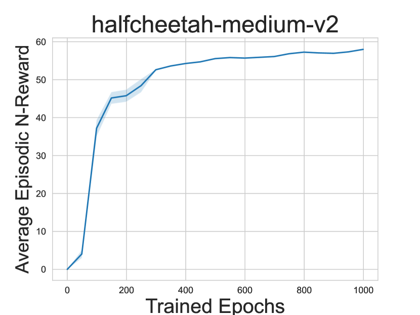
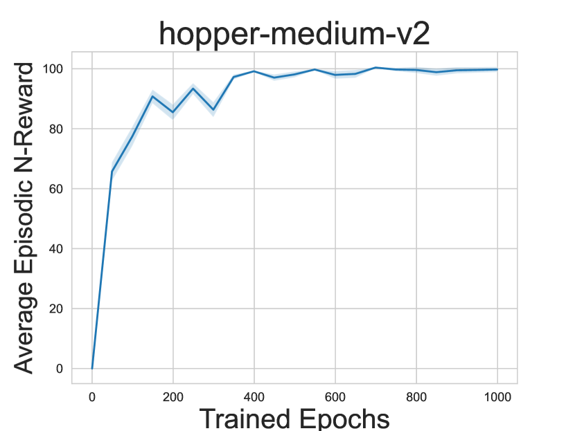
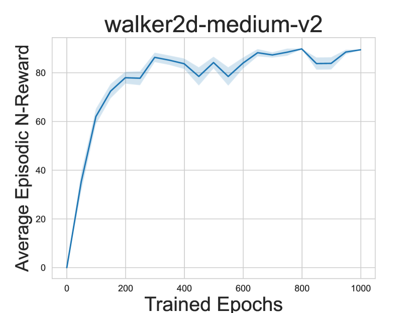
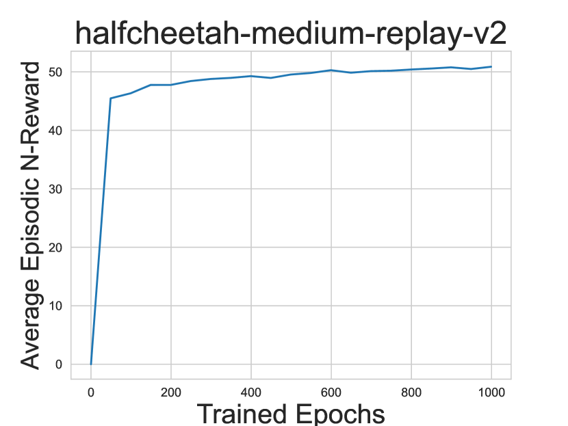
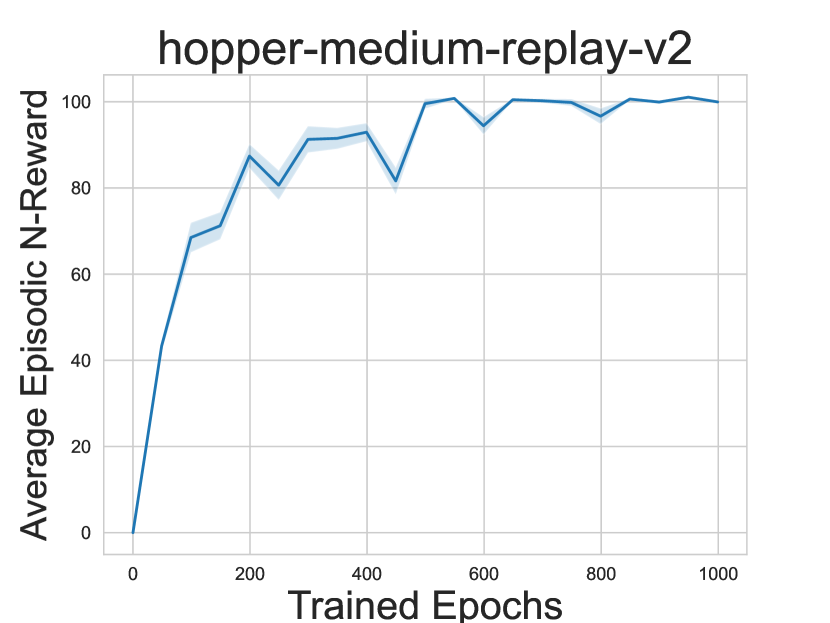
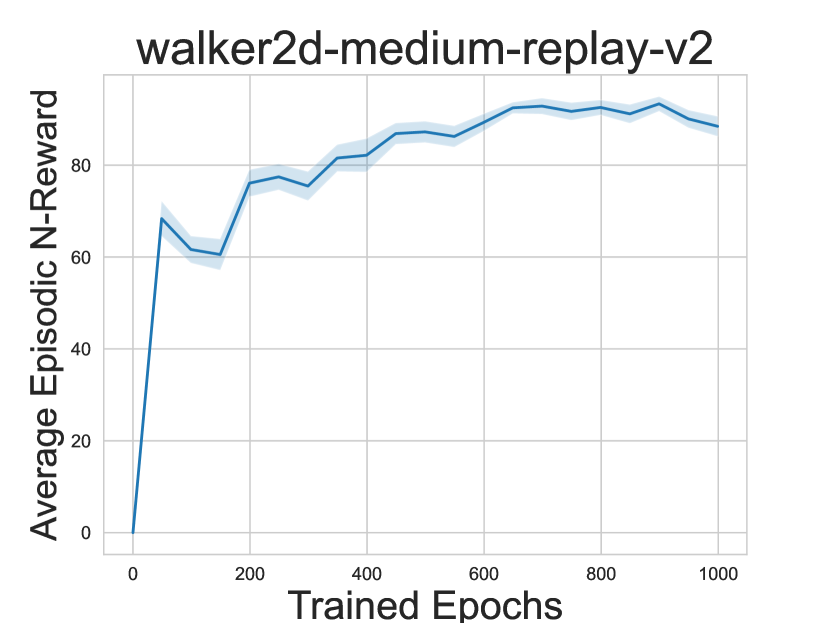
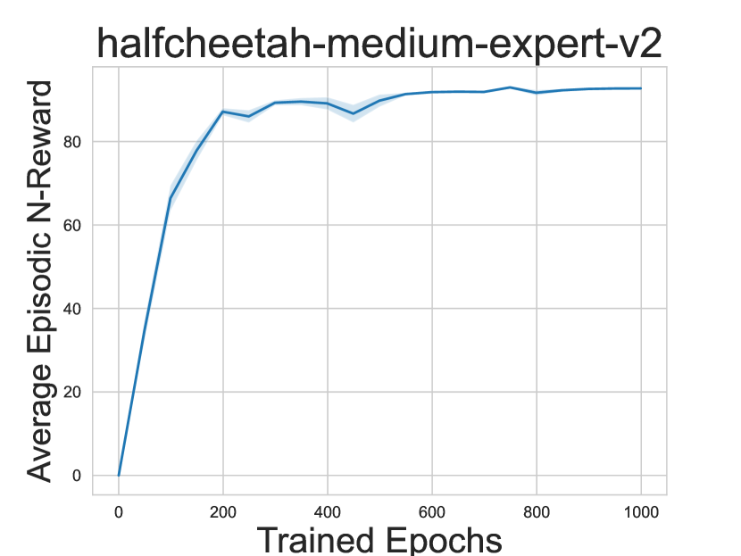
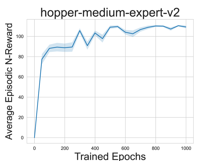
Figure 8: Training curves. Rewards evaluated after every 50 epochs.

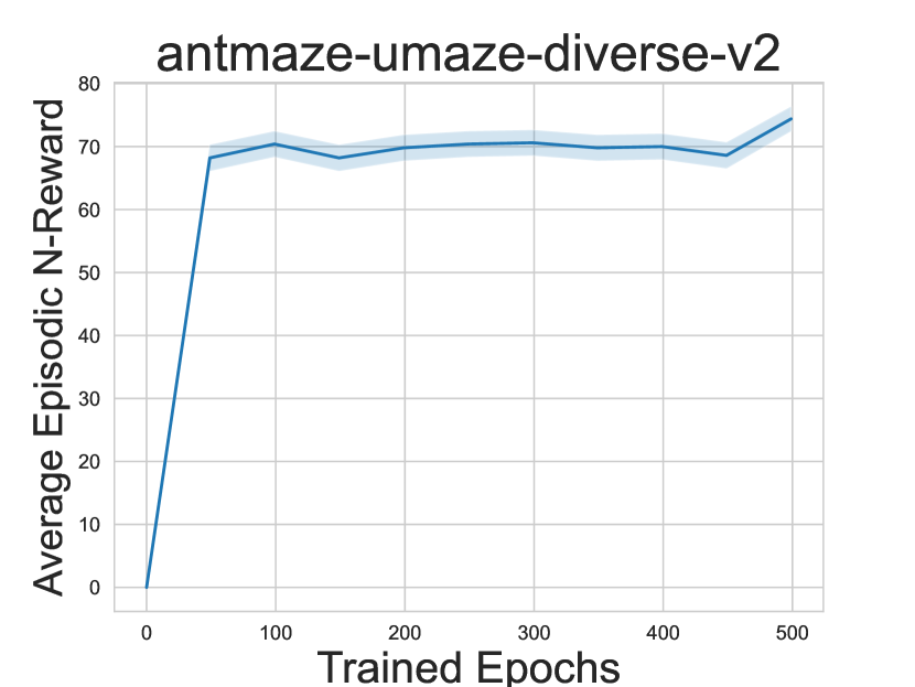
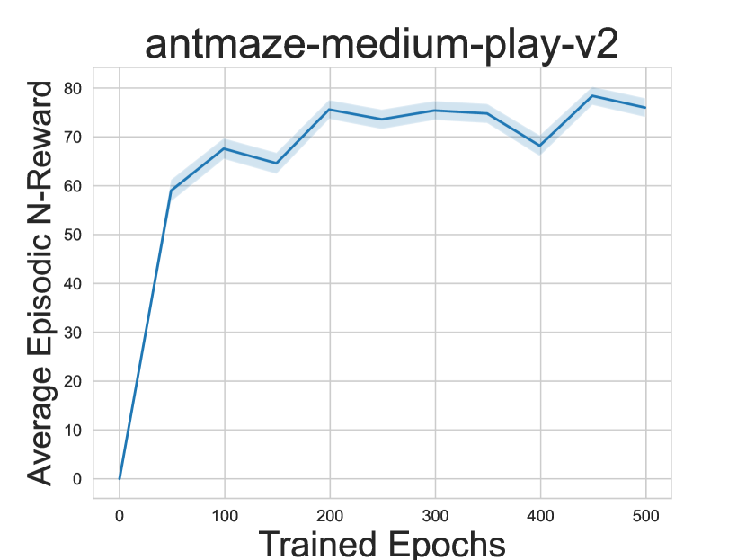
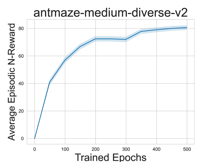
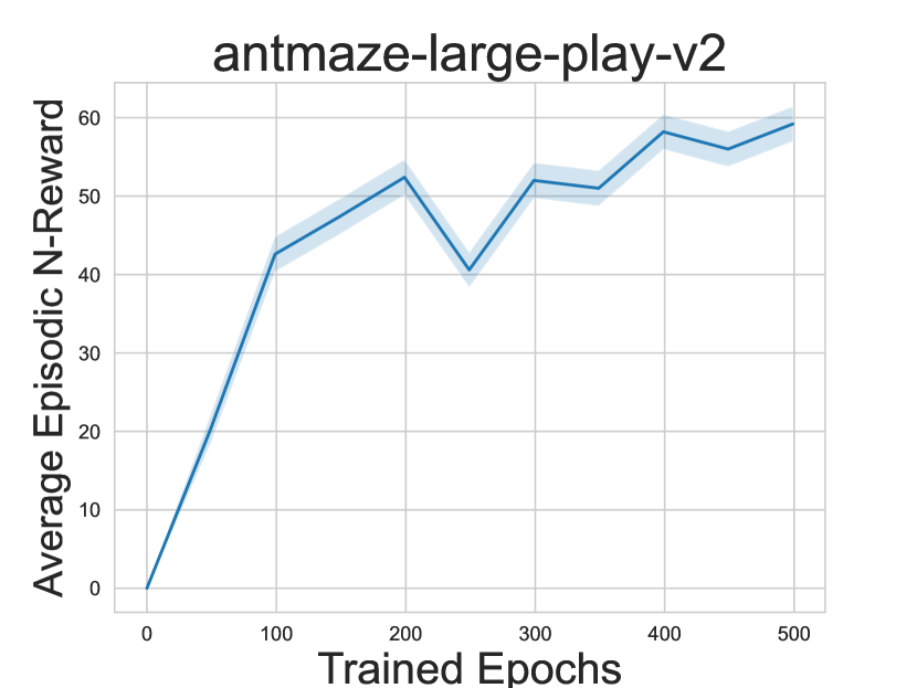
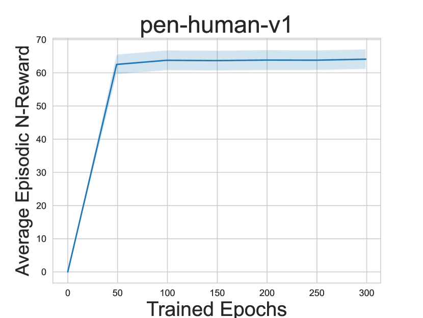
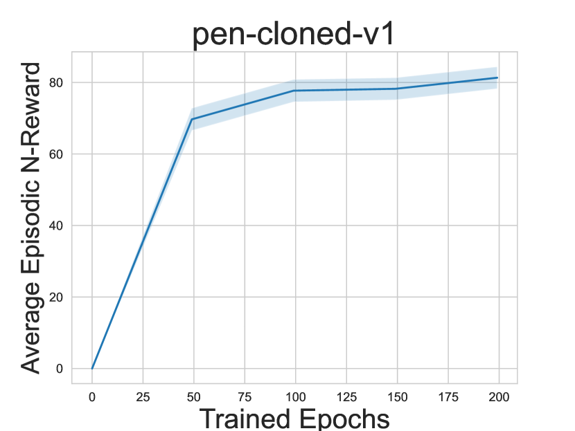
Figure 9: Training curves. Rewards evaluated after every 50 epochs.

References

- Barth-Maron et al. (2018) Gabriel Barth-Maron, Matthew W Hoffman, David Budden, Will Dabney, Dan Horgan, Dhruva Tb, Alistair Muldal, Nicolas Heess, and Timothy Lillicrap. Distributed distributional deterministic policy gradients. arXiv preprint arXiv:1804.08617, 2018.
- Bellemare et al. (2017) Marc G Bellemare, Will Dabney, and Rémi Munos. A distributional perspective on reinforcement learning. In International conference on machine learning, pages 449–458. PMLR, 2017.
- Chen et al. (2022) Huayu Chen, Cheng Lu, Chengyang Ying, Hang Su, and Jun Zhu. Offline reinforcement learning via high-fidelity generative behavior modeling. arXiv preprint arXiv:2209.14548, 2022.
- Chen et al. (2023) Huayu Chen, Cheng Lu, Zhengyi Wang, Hang Su, and Jun Zhu. Score regularized policy optimization through diffusion behavior. arXiv preprint arXiv:2310.07297, 2023.
- Florence et al. (2022) Pete Florence, Corey Lynch, Andy Zeng, Oscar A Ramirez, Ayzaan Wahid, Laura Downs, Adrian Wong, Johnny Lee, Igor Mordatch, and Jonathan Tompson. Implicit behavioral cloning. In Conference on Robot Learning, pages 158–168. PMLR, 2022.
- Fu et al. (2020) Justin Fu, Aviral Kumar, Ofir Nachum, George Tucker, and Sergey Levine. D4RL: Datasets for deep data-driven reinforcement learning. arXiv preprint arXiv:2004.07219, 2020.
- Fujimoto and Gu (2021) Scott Fujimoto and Shixiang Shane Gu. A minimalist approach to offline reinforcement learning. Advances in neural information processing systems, 34:20132–20145, 2021.
- Fujimoto et al. (2019) Scott Fujimoto, David Meger, and Doina Precup. Off-policy deep reinforcement learning without exploration. In International conference on machine learning, pages 2052–2062. PMLR, 2019.
- Ghasemipour et al. (2021) Seyed Kamyar Seyed Ghasemipour, Dale Schuurmans, and Shixiang Shane Gu. EMAQ: Expected-max Q-learning operator for simple yet effective offline and online RL. In International Conference on Machine Learning, pages 3682–3691. PMLR, 2021.
- Goodfellow et al. (2020) Ian Goodfellow, Jean Pouget-Abadie, Mehdi Mirza, Bing Xu, David Warde-Farley, Sherjil Ozair, Aaron Courville, and Yoshua Bengio. Generative adversarial networks. Communications of the ACM, 63(11):139–144, 2020.
- Hansen-Estruch et al. (2023) Philippe Hansen-Estruch, Ilya Kostrikov, Michael Janner, Jakub Grudzien Kuba, and Sergey Levine. IDQL: Implicit Q-learning as an actor-critic method with diffusion policies. arXiv preprint arXiv:2304.10573, 2023.
- Hasselt (2010) Hado Hasselt. Double Q-learning. Advances in neural information processing systems, 23, 2010.
- Ho et al. (2020) Jonathan Ho, Ajay Jain, and Pieter Abbeel. Denoising diffusion probabilistic models. Advances in neural information processing systems, 33:6840–6851, 2020.
- Janner et al. (2022) Michael Janner, Yilun Du, Joshua B Tenenbaum, and Sergey Levine. Planning with diffusion for flexible behavior synthesis. arXiv preprint arXiv:2205.09991, 2022.
- Kang et al. (2024) Bingyi Kang, Xiao Ma, Chao Du, Tianyu Pang, and Shuicheng Yan. Efficient diffusion policies for offline reinforcement learning. Advances in Neural Information Processing Systems, 36, 2024.
- Karras et al. (2022) Tero Karras, Miika Aittala, Timo Aila, and Samuli Laine. Elucidating the design space of diffusion-based generative models. Advances in Neural Information Processing Systems, 35:26565–26577, 2022.
- Kingma and Gao (2024) Diederik Kingma and Ruiqi Gao. Understanding diffusion objectives as the ELBO with simple data augmentation. Advances in Neural Information Processing Systems, 36, 2024.
- Kingma et al. (2021) Diederik Kingma, Tim Salimans, Ben Poole, and Jonathan Ho. Variational diffusion models. Advances in neural information processing systems, 34:21696–21707, 2021.
- Kingma and Welling (2013) Diederik P Kingma and Max Welling. Auto-encoding variational Bayes. arXiv preprint arXiv:1312.6114, 2013.
- Kostrikov et al. (2021) Ilya Kostrikov, Ashvin Nair, and Sergey Levine. Offline reinforcement learning with implicit Q-learning. arXiv preprint arXiv:2110.06169, 2021.
- Kumar et al. (2019) Aviral Kumar, Justin Fu, Matthew Soh, George Tucker, and Sergey Levine. Stabilizing off-policy q-learning via bootstrapping error reduction. Advances in neural information processing systems, 32, 2019.
- Kumar et al. (2020) Aviral Kumar, Aurick Zhou, George Tucker, and Sergey Levine. Conservative Q-learning for offline reinforcement learning. Advances in Neural Information Processing Systems, 33:1179–1191, 2020.
- Lange et al. (2012) Sascha Lange, Thomas Gabel, and Martin Riedmiller. Batch reinforcement learning. In Reinforcement learning: State-of-the-art, pages 45–73. Springer, 2012.
- Li (2017) Yuxi Li. Deep reinforcement learning: An overview. arXiv preprint arXiv:1701.07274, 2017.
- Lu et al. (2022) Cheng Lu, Yuhao Zhou, Fan Bao, Jianfei Chen, Chongxuan Li, and Jun Zhu. DPM-Solver: A fast ODE solver for diffusion probabilistic model sampling in around 10 steps. Advances in Neural Information Processing Systems, 35:5775–5787, 2022.
- Luo et al. (2024) Weijian Luo, Tianyang Hu, Shifeng Zhang, Jiacheng Sun, Zhenguo Li, and Zhihua Zhang. Diff-Instruct: A universal approach for transferring knowledge from pre-trained diffusion models. Advances in Neural Information Processing Systems, 36, 2024.
- Nair et al. (2020) Ashvin Nair, Abhishek Gupta, Murtaza Dalal, and Sergey Levine. Awac: Accelerating online reinforcement learning with offline datasets. arXiv preprint arXiv:2006.09359, 2020.
- Nalisnick et al. (2018) Eric Nalisnick, Akihiro Matsukawa, Yee Whye Teh, Dilan Gorur, and Balaji Lakshminarayanan. Do deep generative models know what they don’t know? arXiv preprint arXiv:1810.09136, 2018.
- Pearce et al. (2023) Tim Pearce, Tabish Rashid, Anssi Kanervisto, Dave Bignell, Mingfei Sun, Raluca Georgescu, Sergio Valcarcel Macua, Shan Zheng Tan, Ida Momennejad, Katja Hofmann, et al. Imitating human behaviour with diffusion models. arXiv preprint arXiv:2301.10677, 2023.
- Poole et al. (2022) Ben Poole, Ajay Jain, Jonathan T Barron, and Ben Mildenhall. DreamFusion: Text-to-3D using 2D diffusion. arXiv preprint arXiv:2209.14988, 2022.
- Song et al. (2020a) Jiaming Song, Chenlin Meng, and Stefano Ermon. Denoising diffusion implicit models. arXiv preprint arXiv:2010.02502, 2020a.
- Song et al. (2020b) Yang Song, Jascha Sohl-Dickstein, Diederik P Kingma, Abhishek Kumar, Stefano Ermon, and Ben Poole. Score-based generative modeling through stochastic differential equations. arXiv preprint arXiv:2011.13456, 2020b.
- Song et al. (2021) Yang Song, Conor Durkan, Iain Murray, and Stefano Ermon. Maximum likelihood training of score-based diffusion models. Advances in neural information processing systems, 34:1415–1428, 2021.
- Wang et al. (2022a) Zhendong Wang, Jonathan J Hunt, and Mingyuan Zhou. Diffusion policies as an expressive policy class for offline reinforcement learning. arXiv preprint arXiv:2208.06193, 2022a.
- Wang et al. (2022b) Zhendong Wang, Huangjie Zheng, Pengcheng He, Weizhu Chen, and Mingyuan Zhou. Diffusion-GAN: Training GANs with diffusion. arXiv preprint arXiv:2206.02262, 2022b.
- Wang et al. (2024) Zhengyi Wang, Cheng Lu, Yikai Wang, Fan Bao, Chongxuan Li, Hang Su, and Jun Zhu. ProlificDreamer: High-fidelity and diverse text-to-3D generation with variational score distillation. Advances in Neural Information Processing Systems, 36, 2024.
- Wiering and Van Otterlo (2012) Marco A Wiering and Martijn Van Otterlo. Reinforcement learning. Adaptation, learning, and optimization, 12(3):729, 2012.
- Wu et al. (2019) Yifan Wu, George Tucker, and Ofir Nachum. Behavior regularized offline reinforcement learning. arXiv preprint arXiv:1911.11361, 2019.
- Yang et al. (2022) Shentao Yang, Zhendong Wang, Huangjie Zheng, Yihao Feng, and Mingyuan Zhou. A behavior regularized implicit policy for offline reinforcement learning. arXiv preprint arXiv:2202.09673, 2022.
- Yin et al. (2023) Tianwei Yin, Michaël Gharbi, Richard Zhang, Eli Shechtman, Fredo Durand, William T Freeman, and Taesung Park. One-step diffusion with distribution matching distillation. arXiv preprint arXiv:2311.18828, 2023.
- Yue et al. (2020) Yuguang Yue, Zhendong Wang, and Mingyuan Zhou. Implicit distributional reinforcement learning. Advances in Neural Information Processing Systems, 33:7135–7147, 2020.
- Zhao et al. (2016) Junbo Zhao, Michael Mathieu, and Yann LeCun. Energy-based generative adversarial network. arXiv preprint arXiv:1609.03126, 2016.
- Zhou et al. (2024) Mingyuan Zhou, Huangjie Zheng, Zhendong Wang, Mingzhang Yin, and Hai Huang. Score identity distillation: Exponentially fast distillation of pretrained diffusion models for one-step generation. In Forty-first International Conference on Machine Learning, 2024. URL https://openreview.net/forum?id=QhqQJqe0Wq.