Uncertainty-guided Optimal Transport in
Depth Supervised Sparse-View 3D Gaussian

Abstract

3D Gaussian splatting has demonstrated impressive performance in real-time novel view synthesis. However, achieving successful reconstruction from RGB images generally requires multiple input views captured under static conditions. To address the challenge of sparse input views, previous approaches have incorporated depth supervision into the training of 3D Gaussians to mitigate overfitting, using dense predictions from pretrained depth networks as pseudo-ground truth. Nevertheless, depth predictions from monocular depth estimation models inherently exhibit significant uncertainty in specific areas. Relying solely on pixel-wise L2 loss may inadvertently incorporate detrimental noise from these uncertain areas. In this work, we introduce a novel method to supervise the depth distribution of 3D Gaussians, utilizing depth priors with integrated uncertainty estimates. To address these localized errors in depth predictions, we integrate a patch-wise optimal transport strategy to complement traditional L2 loss in depth supervision. Extensive experiments conducted on the LLFF, DTU, and Blender datasets demonstrate that our approach, UGOT, achieves superior novel view synthesis and consistently outperforms state-of-the-art methods.

1 Introduction

Novel View Synthesis (NVS) has emerged as a crucial task in 3D computer vision, underpinning advancements in applications ranging from virtual reality to image editing. NVS aims to generate imagery from any viewpoint within a scene, which typically requires meticulous modeling based on multiple scene images. Leveraging implicit scene representations and differentiable volume rendering, Neural Radiance Fields (NeRF) [1] and its derivatives have shown significant progress in this area. However, the NeRF framework is hampered by extensive training and rendering times. While various NeRF variants have managed to accelerate these processes, they often compromise the image quality, particularly in high-resolution renderings.

As an effective alternative, 3D Gaussian splatting (3D-GS) [2] has gained attention for its exceptional training and inference speeds while preserving quality competitive with NeRF. This method employs anisotropic 3D Gaussians and adaptive density controls, enabling precise and explicit scene representations ideal for NVS. Unlike NeRF’s cumbersome volume rendering, 3D-GS utilizes efficient splatting that projects 3D Gaussians onto a 2D plane, facilitating real-time rendering. However, this technique can lead to over-reconstruction in scenes with sparse views due to its localized approach, where large Gaussians might dominate rendering, causing blur and artifacts as well as frequency discrepancies compared to the ground truth.

Previous methods [3, 4] have utilized pixel-wise L2 loss to supervise depth in Gaussian-rendered outputs without considering the variability in depth estimation accuracy across different areas, which can result in misinterpreted geometries. NeRF models, which use implicit representations, benefit from the inherent smoothness of MLPs, thus minor discrepancies in depth do not significantly impact the final rendered image [5]. However, explicit point-based methods like 3D-GS can exacerbate these inaccuracies. Given these challenges, our analysis leads to four key insights:

1. The depth of each pixel in the final render is often determined by a subset of Gaussian splats with the highest weights, negating the need to optimize all Gaussians based on ground truth depth, which can destabilize training due to depth error.

2. The depth estimation’s uncertainty should be explicitly modeled at each image location, thereby primarily utilizing the more reliable depth estimates from areas with lower uncertainty.

3. The L2 loss enforces the rendered depth to exactly replicate the estimated depth prior, potentially leading to overfitting. By supervising the depth distribution of each Gaussian, it is possible to mitigate the impact of noisy depth estimation on scene geometry.

4. Pixel-wise loss tends to exacerbate geometric degradation in areas with high depth uncertainty; therefore, a regional supervision approach should also be adopted to minimize this effect.

Building on these insights, we propose an Uncertainty-guided Optimal Transport (UGOT) approach to optimize the depth distribution of 3DGS patch-wisely. Utilizing off-the-shelf pre-trained generative diffusion models as depth priors, we enhance depth supervision with uncertainty estimates derived during the denoising process. This method prioritizes the use of more reliable depth estimates from areas with lower uncertainty. Additionally, we employ differentiable sampling of the depth distribution from the most influential Gaussian splats and their participation weights. In each iteration, we define random-sized patches, compute patch mean for each set of samples, and incorporate an optimal transport strategy to construct a regional depth distribution loss.

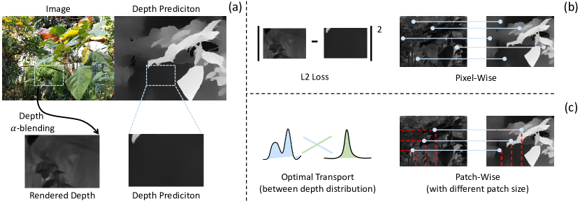
Figure 1: The comparison with the previous method.

2 Related Work

Novel-view Synthesis. Structure from Motion (SfM) [6] and Multi-View Stereo (MVS) [7] are traditional techniques used to reconstruct 3D structures from multiple images and have long been a focus in the computer vision field. For achieving denser and more realistic reconstructions, deep learning-based 3D reconstruction methods have gained prominence [8, 1, 9]. Among these, Neural Radiance Fields (NeRF) [1] stands out as a notable method, utilizing a neural network to represent 3D scenes. NeRF employs an MLP network for 3D space representation and volume rendering, leading to numerous follow-up studies in 3D reconstruction [10, 11, 12, 13, 14, 15]. To address the slow rendering speed of NeRF, considerable efforts have been made to achieve real-time rendering through explicit representations such as sparse voxels [16, 17, 18, 19], featured point clouds [20], tensors [21], and polygons [22]. These representations are composed of local elements that function independently, enabling fast rendering and optimization. Building on this idea, various other representations have been explored, including Multi-Level Hierarchies [23, 24], infinitesimal networks [25, 26], and triplanes [27]. Among these approaches, 3D Gaussian Splatting [2] stands out by representing radiance fields with a set of anisotropic 3D Gaussians and rendering them using differentiable splatting. This technique has achieved significant success in fast and high-quality reconstruction of complex real scenes. While 3D Gaussian Splatting performs excellently with dense input views and has shown success in various 3D tasks [28, 29, 30], its effectiveness in scenarios with sparse view inputs remains an open challenge.

Few-Shot Novel-view Synthesis. The objective of few-shot novel view synthesis is to generate new views from a limited number of sparse input views. Various approaches have been explored to tackle this challenge, with some focusing on regularization strategies specifically tailored for NeRF implementations [31, 32, 33, 34]. Others have ventured into using pre-trained generative models for data augmentation [35, 36, 37, 38, 39], while additional strategies involve leveraging pre-trained models to provide data-driven priors that guide the training regimen [40, 41]. Another significant approach is depth distillation [31, 42, 43, 44], which proves effective in sparse-view neural field applications. Nonetheless, many techniques falter in the context of 3D Gaussian Splatting (3DGS) due to its pronounced locality and the absence of MLP smoothing capabilities. This often results in the existing per-pixel regularization methods failing to effectively address floating artifacts observed when only a few images are available [3].

Depth Supervision in Novel-view Synthesis. Depth cues, long-established as pivotal in various 3D vision applications [45, 46, 47, 48, 49], leading another line of work in guiding novel-view synthesis. Two primary approaches emerge in leveraging depth information. The first approach [31, 42] extracts precise yet sparse depth values from trustworthy point clouds, while the second approach [50, 43, 51, 44, 52] derives depth insights from advanced monocular depth estimators[53, 54, 51]. Although monocular depth estimation addresses the scarcity of point clouds in sparse-view settings, its out-of-domain application introduces challenges such as partial occlusions, shading, and reflections, often resulting in distorted geometries.To mitigate the inherent inaccuracies of monocular depths, prior works in sparse-view synthesis have adopted various scale-invariant losses [55, 43, 52, 56], including depth ranking losses [44, 57]. Furthermore, efforts have been made to model noise and manage uncertain regions [31, 42], alongside the introduction of softer constraints [44] aimed at reducing noise impact. However, these methods do not adequately address the issue of noise within depth-supervised 3D Gaussian contexts. Specifically, the adaptable nature of Gaussians to erroneous depth cues necessitates additional regularization strategies. Moreover, aligning depth to a uniform scale may disregard the influence of noise across various scales. Such oversight can result in a noisy distribution of primitives, especially noticeable in areas with complex textures.

3 Method

An overview of our method is shown in  Figure 2.

3.1 Preliminaries of 3D Gaussian Splatting

3D Gaussian Splatting (3DGS) [2] represents a 3D scene using a suite of 3D Gaussians. The properties of each Gaussian include a 3D position $\mathbf{p}=\{x,y,z\}\in\mathbb{R}^{3}$, a 3D size scaling factor $\mathbf{s}\in\mathbb{R}^{3}$, a rotation quaternion $\mathbf{q}\in\mathbb{R}^{4}$, a color $\mathbf{c}\in\mathbb{R}^{3}$, and an opacity value $o_{i}\in\mathbb{R}$. These parameters are learnable and can be collectively symbolized by $\Gamma_{{\theta}_{i}}=\{\mathbf{p}_{i},\mathbf{s}_{i},\mathbf{q}_{i},\mathbf{c}_{i},o_{i}\}$, where $i$ denotes the $i$-th Gaussian. Specifically, for computing the pixel color ${C}$, it utilizes $\alpha$-blending point-based rendering by blending $\mathcal{N}$ points in the front-to-back depth order:

$${C}=\sum_{i\in\mathcal{N}}T_{i}\alpha_{i}\mathbf{c}_{i},$$ (1)

where $\mathcal{N}$ is the set of Gaussian points that overlap with the given pixel. $\alpha_{i}$ is calculated by $\alpha_{i}=o_{i}G_{i}^{2D}$, where $G_{i}^{2D}$ denotes the function of the $i$-th Gaussian projected onto 2D plane. The transmittance $T_{i}$ is calculated as the product of opacity values of preceding Gaussians that overlap the same pixel: $T_{i}=\prod_{j=1}^{i-1}(1-\alpha_{j})$. The initial 3D Gaussians are constructed from the sparse data points created by Structure-from-Motion (SfM) [6] using COLMAP [58]. To optimize these 3D Gaussians, Gaussian Splatting employs a differentiable rendering technique for projecting them onto the 2D image plane and utilizes gradient-based color supervision to update parameters. The reconstruction loss is computed by minimizing the rendered image $\hat{I}$ and the ground truth image $I$ color, which is formulated as:

$$\mathcal{L}_{rgb}=(1-\lambda)\mathcal{L}_{1}(\hat{I},I)+\lambda\mathcal{L}_{D-SSIM}(\hat{I},I),$$ (2)

where $\lambda$ is set to 0.2. 3DGS has proven effective in 3D reconstruction tasks, showing more efficient inference speeds with high-quality reconstruction comparable to NeRF.

3.2 Optimal Transport (OT)

measures the minimal cost to transport between two probability distributions [59, 60, 61, 62, 63]. We only provide a brief introduction to OT for discrete distributions and refer the readers to [59] for more details. Denote two discrete probability distributions $p=\sum_{i=1}^{n}a_{i}\delta_{x_{i}}$ and $q=\sum_{j=1}^{m}b_{j}\delta_{y_{j}}$, where both $a$ and $b$ are discrete probability vectors summing to 1, $x_{i}$ and $y_{j}$ are the supports of the two distributions respectively, and $\delta$ is a Dirac function. Then the OT distance is formulated as follows: $OT(p,q)=\min_{T\in\Pi(p,q)}\langle T,C\rangle$, where $C\in\mathbb{R}^{n\times m}_{\geq 0}$ is the cost matrix with element $C_{ij}=C(x_{i},y_{j})$ which reflects the cost between $x_{i}$ and $y_{j}$ and the transport probability matrix $T\in\mathbb{R}^{n\times m}_{\geq 0}$ is subject to $\Pi(p,q)=\{T\mid\sum_{i=1}^{n}T_{ij}=b_{j},\sum_{j=1}^{m}T_{ij}=a_{i}\}$. The optimization problem above is often adapted to include a popular entropic regularization term $H=-\sum_{ij}T_{ij}\ln T_{ij}$ for reducing the computational cost, denoted as Sinkhorn algorithm [64].

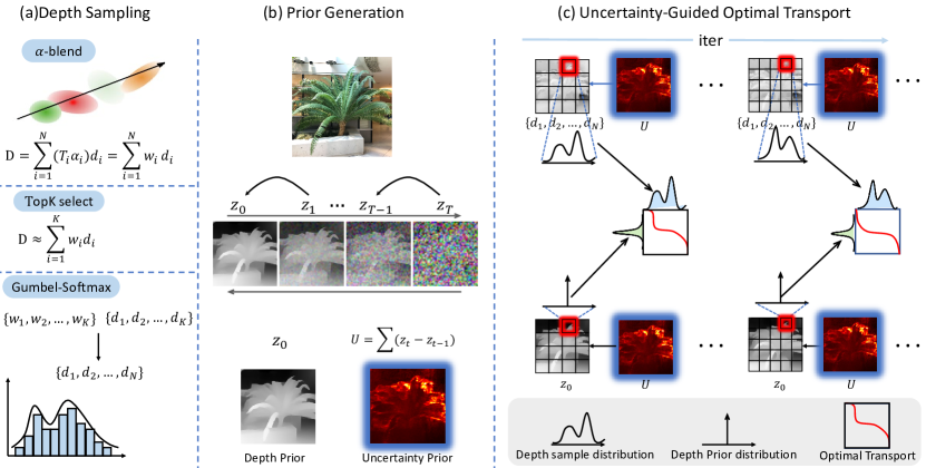
Figure 2: Overview of our method design.

3.2.1 Depth Sampling

In the point-based Gaussian rendering process, each pixel corresponds to a large number of Gaussian primitives that need optimization. However, a significant portion of the information is concentrated in the Gaussians with the highest weights. By extracting the top $K$ Gaussians depth $\tilde{D}_{\text{top}}=\{d_{1},d_{2},\ldots,d_{K}\}$ for each pixel based on their weights $\tilde{W}_{\text{top}}=\{w_{1},w_{2},\ldots,w_{K}\}$, we can reduce the computational and storage burden in distribution optimization, mitigate the drift of smaller Gaussians, improve optimization stability, and enhance overall rendering quality. Specifically, we extract the top $K$ Gaussians for each pixel during the forward pass and sample discrete depth distributions based on their weights and depths using Gumbel-Softmax sampling:

$$p_{j}=\frac{\exp((\log(w_{j})+g_{j})/\tau)}{\sum_{k=1}^{K}\exp((\log(w_{k})+g_{k})/\tau)}$$ (3)

$$d^{*}_{1},d^{*}_{2},\ldots,d^{*}_{n}=\sum_{j=1}^{K}p_{j}d_{j},\quad\text{for }i=1,2,\ldots,n.$$ (4)

where $p_{j}$ is the softmax probability for each depth value $d_{j}$, calculated using Gumbel noise and temperature $\tau$, $g_{j}$ are independent and identically distributed (i.i.d) Gumbel noise variables, $\tau$ is the temperature parameter controlling the softness of the softmax distribution, and $d^{*}_{1},d^{*}_{2},\ldots,d^{*}_{n}$ are the sampled depth values for each pixel, where $n$ is the number of samples.

3.2.2 Optimal Transport for Depth Sampling

In our method, we utilize optimal transport (OT) to compare the sampled depth distribution $D^{*}$ with the ground truth depth $D_{\text{gt}}$ (single value, thus Dirac distribution) provided by a monocular depth estimation model. Given the discrete nature of the sampled depths and the Dirac delta distribution of the ground truth, we formulate the optimal transport problem as follows:

$$OT_{\epsilon}(D^{*},D_{\text{gt}})\stackrel{{\scriptstyle\text{def}}}{{=}}\min_{T_{i}\in\Pi(D^{*},D_{\text{gt}})}\sum_{i}C_{i}T_{i}-\epsilon\left[\sum_{i}T_{i}\ln T_{i}\right]$$ (5)

$$\Pi(D^{*},D_{\text{gt}}):=\left\{T_{i}\ \middle|\ \sum_{i}T_{i}=1,\ T_{i}=w_{i}\right\}$$ (6)

where $D^{*}=\{d_{1}^{*},d_{2}^{*},\ldots,d_{n}^{*}\}$ is the set of sampled depth values, $D_{\text{gt}}$ is the ground truth depth value from the monocular depth estimation model, $\epsilon$ is the hyper-parameter for the entropic constraint, $C_{i}$ is the cost function measuring the difference between $d_{i}^{*}$ and $D_{\text{gt}}$, $T_{i}$ is the transport probability matrix, and $\Pi(D^{*},D_{\text{gt}})$ is the set of all valid transport plans $T_{i}$ that satisfy the marginal constraints.

3.2.3 Patch-wise Optimal Transport

To further enhance the robustness of depth optimization, we introduce a method that aggregates depth estimates over patches. During each iteration, a random patch size from $s_{1}$ to $s_{2}$ is selected. Let $\bar{D}_{\text{patch}}=\{\bar{d}_{1},\bar{d}_{2},\ldots,\bar{d}_{n}\}$ represent the set of mean depth values for a single patch, where each $\bar{d}_{i}$ is the mean of the $i$-th sampled depths within this patch. The optimal transport (OT) problem for each patch is then formulated as:

$$\text{OT}_{\epsilon}(\bar{D}_{\text{patch}},\bar{D}_{gt})=\min_{T\in\Pi(\bar{D}_{\text{patch}},\bar{D}_{gt})}\sum_{i}C_{i}T_{i}-\epsilon\sum_{i}T_{i}\ln T_{i}$$ (7)

$$\Pi(\bar{D}_{\text{patch}},\bar{D}_{gt}):=\left\{T_{i}\mid\sum_{i}T_{i}=1,\ T_{i}=\bar{w}_{i}\right\}$$ (8)

Here, $\Pi(\bar{D}_{\text{patch}},\bar{D}_{gt})$ is the set of admissible transport plans between the depth sample means and their corresponding ground truth mean, $\bar{w}_{i}$ represents the patch mean weight of the $i$-th group of samples and $\bar{D}_{gt}$ represents the patch mean ground truth depth.

3.2.4 Uncertainty-Guided Optimal Transport

As monocular depth estimation is inherently uncertain, it is crucial to measure the confidence in these predictions. While many methods exhibit promising depth prediction capabilities, generative models, especially denoising diffusion models, explicitly illustrates the role of uncertainty in the depth generation process. We adopt the DiffDP model [65], a state-of-the-art diffusion model for depth estimation, which uses image features to denoise noisy depth maps. During inference, features are extracted from the input image, concatenated with random noise, and fed into a lightweight decoder to produce a final depth prediction. Given an input image $\mathbf{I}$, DiffDP formulates the denoising process as:

$$p_{\theta}(z_{0}\mid\mathbf{I})=p_{\theta}(z_{T})\prod_{t=1}^{T}p_{\theta}(z_{t-1}\mid z_{t},\mathbf{I})$$ (9)

where $z_{t}\sim\mathcal{N}(0,\mathbf{I})$ and $z_{0}$ corresponds to the final depth estimate from the model.

During the denoising process, the model updates its estimate recursively. Pixels with higher uncertainty will be updated more frequently, reflecting their instability. This iterative update serves as a proxy for measuring uncertainty in depth estimation. Instead of focusing solely on areas of high error, it captures the intrinsic uncertainty in the depth generation process.

To quantify the uncertainty of a depth estimate $u(z_{0})$, we compare each estimate to the previous one at each time step $t$ and compute the average count of significant changes:

$$c(z_{0}:T)=\frac{1}{T}\sum_{t=T,\ldots,1}\left|z_{t}-z_{t-1}\right|$$ (10)

where $z_{t}$ is the depth prediction at the $T-t$ step.

Let $\mathcal{M}(\cdot)$ denote a function that mirrors an image. The uncertainty for an image $\mathbf{I}$ is then given by:

$$U(z_{0}:T\mid\mathbf{I})=\frac{c(z_{0}:T\mid\mathbf{I})+\mathcal{M}(c(z_{0}:T\mid\mathcal{M}(\mathbf{I})))}{2}$$ (11)

During each iteration, a random patch size $w\times w$ is selected for analysis. The weight maps are normalized within each patch using softmax:

$$W_{\text{patch}}(i)=\text{Softmax}(-U_{\text{patch}}(i))$$ (12)

The weighted mean depth values for the sampled depths and ground truth depths are then computed for each patch:

$$\overline{D}_{\text{patch}}^{U}=\overline{D}_{\text{patch}}\odot W_{\text{patch}}$$ (13)

$$\overline{D}_{\text{gt}}^{U}=\overline{D}_{\text{gt}}\odot W_{\text{patch}}$$ (14)

Finally, the optimal transport problem for the uncertainty-guided mean depths is formulated as:

$$OT_{\epsilon}(\overline{D}_{\text{patch}}^{U},\overline{D}_{\text{gt}}^{U})=\min_{T\in\Pi(\overline{D}_{\text{patch}}^{U},\overline{D}_{\text{gt}}^{U})}\sum_{i}C_{i}T_{i}-\epsilon\sum_{i}T_{i}\ln T_{i}$$ (15)

This framework integrates uncertainty into the depth optimization process, providing more robust depth supervision through meticulously designed weighting, particularly by reducing the impact of depth estimation in uncertain areas.

3.2.5 Training Details

In the supervision of depth estimation, we adopt the per-pixel $L_{2}$ loss on normalized patches from DNGaussian [4], referred to as $L_{\text{dn}}$. Additionally, we employ our proposed uncertainty-guided optimal transport (UGOT), optimizing the cost between distributions using the optimal transport distance, denoted as $L_{\text{ot}}$.

The overall loss function combines these individual components with respective weights:

$$L=\lambda_{1}\cdot L_{\text{dn}}+\lambda_{2}\cdot L_{\text{ot}}+\lambda_{3}\cdot L_{\text{color}}$$ (16)

Where $L_{\text{color}}$ is the RGB-losses in 3D gaussian [2]. By integrating optimal transport loss with per-pixel loss, we utilize the geometric priors within the patch context, while avoiding strictly enforcing rendered depth to exactly replicate depth prediction.

4 Experiments

4.1 Setups

Datasets

We conduct our experiment on three datasets: the NeRF Blender Synthetic dataset (Blender) [1], the DTU dataset [66], and the LLFF dataset [67]. We adhere to the split settings used in previous works [33, 44, 34, 4] to train the model on 3 views and test on another set of images. To minimize background noise and focus on the target object, we apply object masks as used previously [33] for DTU during evaluations. For Blender, our approach is aligned with DietNeRF [40] and FreeNeRF [34], training on 8 views and testing on 25 unseen images. Downsampling rates of 8, 4, and 2 are utilized for LLFF, DTU, and Blender respectively. Camera poses are assumed to be known via calibration or other methods.

Evaluation Metrics

Our evaluation framework utilizes PSNR, SSIM [68], and LPIPS [69] scores to quantitatively assess the reconstruction performance.

Baselines

We compare our results with various current state-of-the-art (SOTA) methods including SRF [70], PixelNeRF [38], MVSNerf [35], Mip-NeRF [10], DietNeRF [40], RegNeRF [33], FreeNeRF [34], and SparseNeRF [44]. Direct comparisons are made with the best quantitative outcomes reported in the literature for these NeRF-based methods. The performance of 3D Gaussian Splattering (3DGS) [2] is also included.

Implementation Details

Our models are constructed using the official PyTorch 3D Gaussian Splattering codebase. We train the models for 6,000 iterations across all datasets. Parameters $\gamma=0.1$ and $\tau=0.95$ are set in the loss functions for all experiments. The hash encoder [4] based neural renderer from [4] is adopted in all 3D Gaussian model for fair comparison. DiffDP [65] is employed to predict monocular depth maps for all input views. The models of 3DGS and DNGaussian are initialized with a uniform distribution.

Table 1: Rendering results. Bold and Underline indicate state-of-the-art (SOTA) and the second best.

Model	LLFF			DTU			Blender
	$\text{PSNR}\uparrow$	$\text{LPIPS}\downarrow$	$\text{SSIM}\uparrow$	$\text{PSNR}\uparrow$	$\text{LPIPS}\downarrow$	$\text{SSIM}\uparrow$	$\text{PSNR}\uparrow$	$\text{LPIPS}\downarrow$	$\text{SSIM}\uparrow$
Mip-NeRF	14.62	0.495	0.351	8.68	0.353	0.571	22.22	0.124	0.851
DietNeRF	14.94	0.496	0.370	11.85	0.314	0.633	23.15	0.109	0.866
RegNeRF	19.08	0.336	0.587	18.89	0.190	0.745	23.83	0.104	0.872
FreeNeRF	19.63	0.308	0.612	19.92	0.182	0.787	24.26	0.098	0.883
SparseNeRF	19.86	0.328	0.624	19.55	0.201	0.769	22.41	0.119	0.861
3DGS	16.46	0.401	0.440	14.74	0.249	0.672	22.23	0.114	0.858
DNGaussian	19.12	0.294	0.591	18.91	0.176	0.790	24.31	0.088	0.886
UGOT(ours)	19.77	0.273	0.625	19.31	0.160	0.808	24.51	0.080	0.899

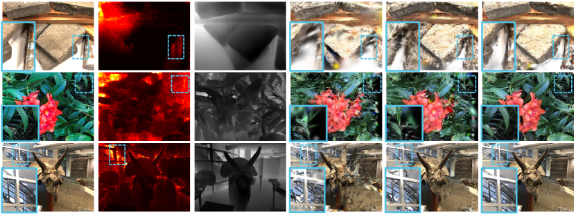
Figure 3: Qualitative results of on DTU and LLFF with 3 input views. From left to right, they are sequentially the original image, the uncertainty map, the depth prediction, 3DGS, DNGaussian and ours.

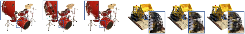
Figure 4: Qualitative results of on Blender with 8 input views. From left to right, they are sequentially the original image, FreeNerf and ours.

Method	FPS	Time	GPU Mem	PSNR$\uparrow$	LPIPS$\downarrow$	SSIM$\uparrow$
FreeNeRF	$9\times 10^{-2}$	2.2 h	$24$ GB	19.92	0.182	0.787
		1.1 h	$24$ GB	19.80	0.189	0.781
SparseNeRF	$9\times 10^{-2}$	1.4 h	$12$ GB	19.55	0.201	0.769
		0.6 h	$12$ GB	19.45	0.207	0.763
DNGaussian	$300$	$3.6$ min	$2$ GB	18.91	0.176	0.790
Ours	$300$	$3.8$ min	$2$ GB	19.31	0.160	0.808

Table 2: Performance comparison of various methods in terms of frame rate (FPS), processing time, GPU memory usage, and image quality metrics (PSNR, LPIPS, SSIM).

4.2 Comparison

DTU Dataset

From three input views, the qualitative results and visualizations on the DTU dataset are shown in  Table 1 and  Figure 3 first row. Our method achieves the best results in LPIPS and SSIM, and ranked second in PSNR, as displayed in  Table 1. Our scores in PSNR are lower compared to FreeNerf and SparseNerf, primarily due to the inherent weaknesses of 3DGS-based methods in reconstructing untextured backgrounds and voids. Yet, the qualitative examples in  Figure 3 illustrate that our approach learns more accurate texture information than DNGaussian and restored high-quality details in areas with significant shadows. This is attributed to our method’s capability to predict higher uncertainty in shadow regions, utilizing context information to smooth the results instead of pixel-wisely relying on inaccurate depth data.

LLFF Dataset

In the three-view setting of LLFF,  Table 1 shows that our method generally achieves the best results. As the NeRF-based benchmarks interpolate colors into invisible areas, whereas the discrete Gaussian radiance field methods directly expose the black background in these areas, methods based on 3DGS naturally have a disadvantage in reconstructing metrics from these invisible areas. Nevertheless, our approach still surpasses all baselines in the LPIPS and SSIM and are comparable in PSNR to the best methods.  Figure 3, rows two and three, presents qualitative outcomes showing our method’s ability to predict higher uncertainty in severely defocused (second row) and highly reflective areas along with object edges (third row). Our method employs optimal transport to avoid directly enforcing depth maps to resemble their depth prior, thereby stably enhancing the rendering quality.

Blender Dataset

We conduct an evaluation on the Blender dataset with eight input views. Our method surpass all other methods in SSIM, LPIPS and even PSNR scores. Although FreeNerf intricately tunes some texture-rich parts through modulation of frequency information, it still fails in areas with complex textures. Our qualitative analysis in  Figure 4 effectively illustrates this point. Our approach leads to less severe artifacts, and crisper and more accurate edges in RGB renderings.

Efficiency

We further conduct an efficiency study on the DTU 3-view setting with an RTX 3090 GPU to explore the performance of current SOTA baselines. As shown in  Table 2, with only 1.1 times the training time, achieves significant performance improvements over DNGaussian. The rendering speed remains unchanged since we are not altering the rendering logic. This also means that, relative to NeRF-based methods, we achieves more than a 1000-fold improvement in rendering speed while nearly matching the performance in quality.

4.3 Ablation Study

Table 3: Ablation Study

	LLFF			DTU
	PSNR $\uparrow$	LPIPS $\downarrow$	SSIM $\uparrow$	PSNR $\uparrow$	LPIPS $\downarrow$	SSIM $\uparrow$
Baseline [4]	19.12	0.294	0.591	18.91	0.176	0.790
+pixel-wise OT	19.08	0.299	0.581	18.79	0.185	0.779
+patch-wise OT	19.36	0.288	0.604	19.08	0.166	0.800
+uncertainty-guided OT (ours)	19.77	0.273	0.625	19.31	0.160	0.808
uncertainty-guided OT (w/o L2)	19.08	0.306	0.577	18.82	0.190	0.771

Ablation on core components.

In  Table 3, we set DNGaussian [4] (with our depth estimation) as baseline and evaluate the impact of each proposed component on the model’s performance. While completely removing the pixel-wise L2 loss does not achieve optimal results, and even performs worse than the baseline, our method effectively mitigates the amplification of local errors in depth prediction that typically occurs in 3D gaussain based methods. By integrating L2 loss, our approach maximizes the utilization of depth information, thus achieving superior performance.

Analysis of TopK values.

Table 4: TopK values Analysis

TopK	Total weight	PSNR $\uparrow$	LPIPS $\downarrow$	SSIM $\uparrow$
K=1	9.8%	18.72	309	0.564
K=5	13.96%	18.99	0.294	0.580
K=10	27.04%	19.27	0.288	0.592
K=20	52.91%	19.77	0.273	0.625
K=40	63.09%	19.62	0.277	0.619

In  Table 4, we further investigate the effectiveness of different TopK values on LLFF. With smaller values of K, back propagation affects fewer Gaussians, and a limited number of Gaussians do not adequately reconstruct the scene’s geometry. However, as the value of K increases, the total weight of the most significant Gaussians exceeds 50%, and updating only these Gaussians during back propagation can already prevent overfitting. Nonetheless, as K continues to increase, the jitter effect of fitting distributions becomes apparent, leading to each pixel’s rendering error affecting many Gaussians, which furthur amplifies the error effect in depth prediction.

Analysis of uncertainty.

Table 5: Uncertainty Analysis

Uncertainty	Sign	PSNR $\uparrow$
plain	-	18.88
	+	19.15
exponential	-	18.92
	+	19.49
softmax	-	19.22
	+	19.77

In  Table 5, we further explore the effectiveness of computed uncertainties on LLFF. Direct use of diffusion-based uncertainty predictions (plain) does not significantly alter performance. However, modulation through exponential or softmax approaches, especially using softmax within patches, yields the best results. By mistakenly using the uncertainty as "certainty" through negation of the signs, we observed a significant drop in performance, further validating the logical soundness of our uncertainty design.

5 Conclusion

In this paper, we present the Uncertainty-guided Optimal Transport (UGOT) for depth supervision in sparse-view 3D Gaussian splatting for novel view synthesis. Our approach integrates uncertainty estimates with depth priors to selectively reducing depth supervision in areas of lower uncertainty, and employs an optimal transport framework to align the depth distribution closer to the ground truth. Extensive experiments on the LLFF, DTU, and Blender datasets demonstrate that UGOT significantly outperforms existing methods as well as achieves faster convergence and superior real-time rendering quality. This validates UGOT as an effective solution for enhancing novel view synthesis under conditions of sparse input views and variable depth certainty.

References

- [1] Ben Mildenhall, Pratul P Srinivasan, Matthew Tancik, Jonathan T Barron, Ravi Ramamoorthi, and Ren Ng. Nerf: Representing scenes as neural radiance fields for view synthesis. Communications of the ACM, 65(1):99–106, 2021.
- [2] Bernhard Kerbl, Georgios Kopanas, Thomas Leimkühler, and George Drettakis. 3d gaussian splatting for real-time radiance field rendering. ACM Transactions on Graphics, 42(4):1–14, 2023.
- [3] Jaeyoung Chung, Jeongtaek Oh, and Kyoung Mu Lee. Depth-regularized optimization for 3d gaussian splatting in few-shot images. arXiv preprint arXiv:2311.13398, 2023.
- [4] Jiahe Li, Jiawei Zhang, Xiao Bai, Jin Zheng, Xin Ning, Jun Zhou, and Lin Gu. Dngaussian: Optimizing sparse-view 3d gaussian radiance fields with global-local depth normalization. arXiv preprint arXiv:2403.06912, 2024.
- [5] Anita Rau, Josiah Aklilu, F Christopher Holsinger, and Serena Yeung-Levy. Depth-guided nerf training via earth mover’s distance. arXiv preprint arXiv:2403.13206, 2024.
- [6] Shimon Ullman. The interpretation of structure from motion. Proceedings of the Royal Society of London. Series B. Biological Sciences, 203(1153):405–426, 1979.
- [7] Carlo Tomasi and Takeo Kanade. Shape and motion from image streams under orthography: a factorization method. International journal of computer vision, 9:137–154, 1992.
- [8] Xian-Feng Han, Hamid Laga, and Mohammed Bennamoun. Image-based 3d object reconstruction: State-of-the-art and trends in the deep learning era. IEEE transactions on pattern analysis and machine intelligence, 43(5):1578–1604, 2019.
- [9] Yiheng Xie, Towaki Takikawa, Shunsuke Saito, Or Litany, Shiqin Yan, Numair Khan, Federico Tombari, James Tompkin, Vincent Sitzmann, and Srinath Sridhar. Neural fields in visual computing and beyond. In Computer Graphics Forum, volume 41, pages 641–676. Wiley Online Library, 2022.
- [10] Jonathan T Barron, Ben Mildenhall, Matthew Tancik, Peter Hedman, Ricardo Martin-Brualla, and Pratul P Srinivasan. Mip-nerf: A multiscale representation for anti-aliasing neural radiance fields. In Proceedings of the IEEE/CVF International Conference on Computer Vision, pages 5855–5864, 2021.
- [11] Jonathan T Barron, Ben Mildenhall, Dor Verbin, Pratul P Srinivasan, and Peter Hedman. Mip-nerf 360: Unbounded anti-aliased neural radiance fields. In Proceedings of the IEEE/CVF Conference on Computer Vision and Pattern Recognition, pages 5470–5479, 2022.
- [12] Kyle Gao, Yina Gao, Hongjie He, Dening Lu, Linlin Xu, and Jonathan Li. Nerf: Neural radiance field in 3d vision, a comprehensive review. arXiv preprint arXiv:2210.00379, 2022.
- [13] Ayush Tewari, Justus Thies, Ben Mildenhall, Pratul Srinivasan, Edgar Tretschk, Wang Yifan, Christoph Lassner, Vincent Sitzmann, Ricardo Martin-Brualla, Stephen Lombardi, et al. Advances in neural rendering. In Computer Graphics Forum, volume 41, pages 703–735. Wiley Online Library, 2022.
- [14] Peng Wang, Lingjie Liu, Yuan Liu, Christian Theobalt, Taku Komura, and Wenping Wang. Neus: Learning neural implicit surfaces by volume rendering for multi-view reconstruction. arXiv preprint arXiv:2106.10689, 2021.
- [15] Lior Yariv, Jiatao Gu, Yoni Kasten, and Yaron Lipman. Volume rendering of neural implicit surfaces. Advances in Neural Information Processing Systems, 34:4805–4815, 2021.
- [16] Sara Fridovich-Keil, Alex Yu, Matthew Tancik, Qinhong Chen, Benjamin Recht, and Angjoo Kanazawa. Plenoxels: Radiance fields without neural networks. In Proceedings of the IEEE/CVF Conference on Computer Vision and Pattern Recognition, pages 5501–5510, 2022.
- [17] Lingjie Liu, Jiatao Gu, Kyaw Zaw Lin, Tat-Seng Chua, and Christian Theobalt. Neural sparse voxel fields. Advances in Neural Information Processing Systems, 33:15651–15663, 2020.
- [18] Cheng Sun, Min Sun, and Hwann-Tzong Chen. Direct voxel grid optimization: Super-fast convergence for radiance fields reconstruction. In Proceedings of the IEEE/CVF Conference on Computer Vision and Pattern Recognition, pages 5459–5469, 2022.
- [19] Alex Yu, Ruilong Li, Matthew Tancik, Hao Li, Ren Ng, and Angjoo Kanazawa. Plenoctrees for real-time rendering of neural radiance fields. In Proceedings of the IEEE/CVF International Conference on Computer Vision, pages 5752–5761, 2021.
- [20] Qiangeng Xu, Zexiang Xu, Julien Philip, Sai Bi, Zhixin Shu, Kalyan Sunkavalli, and Ulrich Neumann. Point-nerf: Pointbased neural radiance fields. 2022 ieee. In CVF Conference on Computer Vision and Pattern Recognition (CVPR), pages 5428–5438, 2022.
- [21] Anpei Chen, Zexiang Xu, Andreas Geiger, Jingyi Yu, and Hao Su. Tensorf: Tensorial radiance fields. In European Conference on Computer Vision, pages 333–350. Springer, 2022.
- [22] Zhiqin Chen, Thomas Funkhouser, Peter Hedman, and Andrea Tagliasacchi. Mobilenerf: Exploiting the polygon rasterization pipeline for efficient neural field rendering on mobile architectures. In Proceedings of the IEEE/CVF Conference on Computer Vision and Pattern Recognition, pages 16569–16578, 2023.
- [23] Thomas Müller, Fabrice Rousselle, Jan Novák, and Alexander Keller. Real-time neural radiance caching for path tracing. arXiv preprint arXiv:2106.12372, 2021.
- [24] Thomas Müller, Alex Evans, Christoph Schied, and Alexander Keller. Instant neural graphics primitives with a multiresolution hash encoding. ACM transactions on graphics (TOG), 41(4):1–15, 2022.
- [25] Stephan J Garbin, Marek Kowalski, Matthew Johnson, Jamie Shotton, and Julien Valentin. Fastnerf: High-fidelity neural rendering at 200fps. In Proceedings of the IEEE/CVF international conference on computer vision, pages 14346–14355, 2021.
- [26] Christian Reiser, Songyou Peng, Yiyi Liao, and Andreas Geiger. Kilonerf: Speeding up neural radiance fields with thousands of tiny mlps. In Proceedings of the IEEE/CVF international conference on computer vision, pages 14335–14345, 2021.
- [27] Eric R Chan, Connor Z Lin, Matthew A Chan, Koki Nagano, Boxiao Pan, Shalini De Mello, Orazio Gallo, Leonidas J Guibas, Jonathan Tremblay, Sameh Khamis, et al. Efficient geometry-aware 3d generative adversarial networks. In Proceedings of the IEEE/CVF conference on computer vision and pattern recognition, pages 16123–16133, 2022.
- [28] Ruoshi Liu, Rundi Wu, Basile Van Hoorick, Pavel Tokmakov, Sergey Zakharov, and Carl Vondrick. Zero-1-to-3: Zero-shot one image to 3d object. In Proceedings of the IEEE/CVF International Conference on Computer Vision, pages 9298–9309, 2023.
- [29] Jiaxiang Tang, Jiawei Ren, Hang Zhou, Ziwei Liu, and Gang Zeng. Dreamgaussian: Generative gaussian splatting for efficient 3d content creation. arXiv preprint arXiv:2309.16653, 2023.
- [30] Guanjun Wu, Taoran Yi, Jiemin Fang, Lingxi Xie, Xiaopeng Zhang, Wei Wei, Wenyu Liu, Qi Tian, and Xinggang Wang. 4d gaussian splatting for real-time dynamic scene rendering. arXiv preprint arXiv:2310.08528, 2023.
- [31] Kangle Deng, Andrew Liu, Jun-Yan Zhu, and Deva Ramanan. Depth-supervised nerf: Fewer views and faster training for free. In Proceedings of the IEEE/CVF Conference on Computer Vision and Pattern Recognition, pages 12882–12891, 2022.
- [32] Mijeong Kim, Seonguk Seo, and Bohyung Han. Infonerf: Ray entropy minimization for few-shot neural volume rendering. In Proceedings of the IEEE/CVF Conference on Computer Vision and Pattern Recognition, pages 12912–12921, 2022.
- [33] Michael Niemeyer, Jonathan T Barron, Ben Mildenhall, Mehdi SM Sajjadi, Andreas Geiger, and Noha Radwan. Regnerf: Regularizing neural radiance fields for view synthesis from sparse inputs. In Proceedings of the IEEE/CVF Conference on Computer Vision and Pattern Recognition, pages 5480–5490, 2022.
- [34] Jiawei Yang, Marco Pavone, and Yue Wang. Freenerf: Improving few-shot neural rendering with free frequency regularization. In Proceedings of the IEEE/CVF Conference on Computer Vision and Pattern Recognition, pages 8254–8263, 2023.
- [35] Anpei Chen, Zexiang Xu, Fuqiang Zhao, Xiaoshuai Zhang, Fanbo Xiang, Jingyi Yu, and Hao Su. Mvsnerf: Fast generalizable radiance field reconstruction from multi-view stereo. In Proceedings of the IEEE/CVF international conference on computer vision, pages 14124–14133, 2021.
- [36] Wenyan Cong, Hanxue Liang, Peihao Wang, Zhiwen Fan, Tianlong Chen, Mukund Varma, Yi Wang, and Zhangyang Wang. Enhancing nerf akin to enhancing llms: Generalizable nerf transformer with mixture-of-view-experts. In Proceedings of the IEEE/CVF International Conference on Computer Vision, pages 3193–3204, 2023.
- [37] Jonáš Kulhánek, Erik Derner, Torsten Sattler, and Robert Babuška. Viewformer: Nerf-free neural rendering from few images using transformers. In European Conference on Computer Vision, pages 198–216. Springer, 2022.
- [38] Alex Yu, Vickie Ye, Matthew Tancik, and Angjoo Kanazawa. pixelnerf: Neural radiance fields from one or few images. In Proceedings of the IEEE/CVF Conference on Computer Vision and Pattern Recognition, pages 4578–4587, 2021.
- [39] Zhizhuo Zhou and Shubham Tulsiani. Sparsefusion: Distilling view-conditioned diffusion for 3d reconstruction. In Proceedings of the IEEE/CVF Conference on Computer Vision and Pattern Recognition, pages 12588–12597, 2023.
- [40] Ajay Jain, Matthew Tancik, and Pieter Abbeel. Putting nerf on a diet: Semantically consistent few-shot view synthesis. In Proceedings of the IEEE/CVF International Conference on Computer Vision, pages 5885–5894, 2021.
- [41] Jamie Wynn and Daniyar Turmukhambetov. Diffusionerf: Regularizing neural radiance fields with denoising diffusion models. In Proceedings of the IEEE/CVF Conference on Computer Vision and Pattern Recognition, pages 4180–4189, 2023.
- [42] Barbara Roessle, Jonathan T Barron, Ben Mildenhall, Pratul P Srinivasan, and Matthias Nießner. Dense depth priors for neural radiance fields from sparse input views. In Proceedings of the IEEE/CVF Conference on Computer Vision and Pattern Recognition, pages 12892–12901, 2022.
- [43] Jiuhn Song, Seonghoon Park, Honggyu An, Seokju Cho, Min-Seop Kwak, Sungjin Cho, and Seungryong Kim. Därf: Boosting radiance fields from sparse input views with monocular depth adaptation. Advances in Neural Information Processing Systems, 36, 2024.
- [44] Guangcong Wang, Zhaoxi Chen, Chen Change Loy, and Ziwei Liu. Sparsenerf: Distilling depth ranking for few-shot novel view synthesis. In Proceedings of the IEEE/CVF International Conference on Computer Vision, pages 9065–9076, 2023.
- [45] Chen Wang, Xiang Wang, Jiawei Zhang, Liang Zhang, Xiao Bai, Xin Ning, Jun Zhou, and Edwin Hancock. Uncertainty estimation for stereo matching based on evidential deep learning. Pattern Recognition, 124:108498, 2022.
- [46] Xiang Wang, Chen Wang, Bing Liu, Xiaoqing Zhou, Liang Zhang, Jin Zheng, and Xiao Bai. Multi-view stereo in the deep learning era: A comprehensive review. Displays, 70:102102, 2021.
- [47] Zihang Wang, Haonan Luo, Xiang Wang, Jin Zheng, Xin Ning, and Xiao Bai. A contrastive learning based unsupervised multi-view stereo with multi-stage self-training strategy. Displays, page 102672, 2024.
- [48] Xiang Wang, Haonan Luo, Zihang Wang, Jin Zheng, and Xiao Bai. Robust training for multi-view stereo networks with noisy labels. Displays, 81:102604, 2024.
- [49] Jiawei Zhang, Xiang Wang, Xiao Bai, Chen Wang, Lei Huang, Yimin Chen, Lin Gu, Jun Zhou, Tatsuya Harada, and Edwin R Hancock. Revisiting domain generalized stereo matching networks from a feature consistency perspective. In Proceedings of the IEEE/CVF Conference on Computer Vision and Pattern Recognition, pages 13001–13011, 2022.
- [50] Shoukang Hu, Kaichen Zhou, Kaiyu Li, Longhui Yu, Lanqing Hong, Tianyang Hu, Zhenguo Li, Gim Hee Lee, and Ziwei Liu. Consistentnerf: Enhancing neural radiance fields with 3d consistency for sparse view synthesis. arXiv preprint arXiv:2305.11031, 2023.
- [51] Mikaela Angelina Uy, Ricardo Martin-Brualla, Leonidas Guibas, and Ke Li. Scade: Nerfs from space carving with ambiguity-aware depth estimates. In Proceedings of the IEEE/CVF Conference on Computer Vision and Pattern Recognition, pages 16518–16527, 2023.
- [52] Zehao Yu, Songyou Peng, Michael Niemeyer, Torsten Sattler, and Andreas Geiger. Monosdf: Exploring monocular geometric cues for neural implicit surface reconstruction. Advances in neural information processing systems, 35:25018–25032, 2022.
- [53] René Ranftl, Alexey Bochkovskiy, and Vladlen Koltun. Vision transformers for dense prediction. In Proceedings of the IEEE/CVF international conference on computer vision, pages 12179–12188, 2021.
- [54] René Ranftl, Katrin Lasinger, David Hafner, Konrad Schindler, and Vladlen Koltun. Towards robust monocular depth estimation: Mixing datasets for zero-shot cross-dataset transfer. IEEE transactions on pattern analysis and machine intelligence, 44(3):1623–1637, 2020.
- [55] Congyue Deng, Chiyu Jiang, Charles R Qi, Xinchen Yan, Yin Zhou, Leonidas Guibas, Dragomir Anguelov, et al. Nerdi: Single-view nerf synthesis with language-guided diffusion as general image priors. In Proceedings of the IEEE/CVF Conference on Computer Vision and Pattern Recognition, pages 20637–20647, 2023.
- [56] Zehao Zhu, Zhiwen Fan, Yifan Jiang, and Zhangyang Wang. Fsgs: Real-time few-shot view synthesis using gaussian splatting. arXiv preprint arXiv:2312.00451, 2023.
- [57] Dejia Xu, Yifan Jiang, Peihao Wang, Zhiwen Fan, Yi Wang, and Zhangyang Wang. Neurallift-360: Lifting an in-the-wild 2d photo to a 3d object with 360deg views. In Proceedings of the IEEE/CVF Conference on Computer Vision and Pattern Recognition, pages 4479–4489, 2023.
- [58] Johannes L Schonberger and Jan-Michael Frahm. Structure-from-motion revisited. In Proceedings of the IEEE conference on computer vision and pattern recognition, pages 4104–4113, 2016.
- [59] Gabriel Peyré, Marco Cuturi, et al. Computational optimal transport: With applications to data science. Foundations and Trends® in Machine Learning, 11(5-6):355–607, 2019.
- [60] Jean-David Benamou, Guillaume Carlier, Marco Cuturi, Luca Nenna, and Gabriel Peyré. Iterative bregman projections for regularized transportation problems. SIAM Journal on Scientific Computing, 37(2):A1111–A1138, 2015.
- [61] Lenaic Chizat, Gabriel Peyré, Bernhard Schmitzer, and François-Xavier Vialard. Scaling algorithms for unbalanced optimal transport problems. Mathematics of Computation, 87(314):2563–2609, 2018.
- [62] Nicolas Courty, Rémi Flamary, Devis Tuia, and Alain Rakotomamonjy. Optimal transport for domain adaptation. IEEE transactions on pattern analysis and machine intelligence, 39(9):1853–1865, 2016.
- [63] Aude Genevay, Marco Cuturi, Gabriel Peyré, and Francis Bach. Stochastic optimization for large-scale optimal transport. Advances in neural information processing systems, 29, 2016.
- [64] Marco Cuturi. Sinkhorn distances: Lightspeed computation of optimal transport. Advances in neural information processing systems, 26, 2013.
- [65] Yuanfeng Ji, Zhe Chen, Enze Xie, Lanqing Hong, Xihui Liu, Zhaoqiang Liu, Tong Lu, Zhenguo Li, and Ping Luo. Ddp: Diffusion model for dense visual prediction. In Proceedings of the IEEE/CVF International Conference on Computer Vision, pages 21741–21752, 2023.
- [66] Rasmus Jensen, Anders Dahl, George Vogiatzis, Engin Tola, and Henrik Aanæs. Large scale multi-view stereopsis evaluation. In Proceedings of the IEEE conference on computer vision and pattern recognition, pages 406–413, 2014.
- [67] Ben Mildenhall, Pratul P Srinivasan, Rodrigo Ortiz-Cayon, Nima Khademi Kalantari, Ravi Ramamoorthi, Ren Ng, and Abhishek Kar. Local light field fusion: Practical view synthesis with prescriptive sampling guidelines. ACM Transactions on Graphics (TOG), 38(4):1–14, 2019.
- [68] Zhou Wang, Alan C Bovik, Hamid R Sheikh, and Eero P Simoncelli. Image quality assessment: from error visibility to structural similarity. IEEE transactions on image processing, 13(4):600–612, 2004.
- [69] Richard Zhang, Phillip Isola, Alexei A Efros, Eli Shechtman, and Oliver Wang. The unreasonable effectiveness of deep features as a perceptual metric. In Proceedings of the IEEE conference on computer vision and pattern recognition, pages 586–595, 2018.
- [70] Julian Chibane, Aayush Bansal, Verica Lazova, and Gerard Pons-Moll. Stereo radiance fields (srf): Learning view synthesis for sparse views of novel scenes. In Proceedings of the IEEE/CVF Conference on Computer Vision and Pattern Recognition, pages 7911–7920, 2021.